communication systems lab manual
TRANSCRIPT
SPSU, UDAIPUR Lab Manual Department of E & C Engineering
1
SCHOOL OF ENGINEERINGSCHOOL OF ENGINEERINGSCHOOL OF ENGINEERINGSCHOOL OF ENGINEERING
UDAIPURUDAIPURUDAIPURUDAIPUR
LABORATORY MANUALLABORATORY MANUALLABORATORY MANUALLABORATORY MANUAL
ANALOG COMMUNICATION ANALOG COMMUNICATION ANALOG COMMUNICATION ANALOG COMMUNICATION LABLABLABLAB
ECECECEC----205205205205
DEDEDEDEPARTMENT OF ELECTRONICS & COMMUNICATION PARTMENT OF ELECTRONICS & COMMUNICATION PARTMENT OF ELECTRONICS & COMMUNICATION PARTMENT OF ELECTRONICS & COMMUNICATION
ENGINEERINGENGINEERINGENGINEERINGENGINEERING
SPSU, UDAIPUR Lab Manual Department of E & C Engineering
2
ANALOG COMMUNICATION LAB
This laboratory will commence with ‘Orientations’ to familiarize students with surroundings or circumstances includes following: A. Familiarization with MATLAB and its communication toolbox B. Familiarization amplitude modulation, frequency modulation and super heterodyne
AM receiver.
S. N. Title of the Experiment
1 To study MATLAB and communication tool box
2 To generate AM wave without using matlab inbuilt function
3 To generate AM wave and plot it’s frequency spectrum using matlab
4 To generate AM wave for different value of modulation index(m<1, m=1 & m>1) using matlab
5 To generate FM wave and plot it’s frequency spectrum using matlab
6 To generate Amplitude Modulation (AM) wave and determine it’s Modulation Index ‘ma’
7 To demodulate amplitude modulated wave
8 To generate frequency modulation wave
9 To demodulate frequency modulated wave
10 To study super heterodyne AM receiver
SPSU, UDAIPUR Lab Manual Department of E & C Engineering
3
LIST OF EXPERIMENTS
NAME OF THE STUDENT………………………………………. ENROLL. NO…………………………
INDEX
S. N. Name of the experiment Page no.
Date of allotment
Date of conduction
Sign /grade
1 To study MATLAB and communication tool box
2 To generate AM wave without using matlab inbuilt function
3 To generate AM wave and plot it’s frequency spectrum using matlab
4 To generate AM wave for different value of modulation index(m<1, m=1 & m>1) using matlab
5 To generate FM wave and plot it’s frequency spectrum using matlab
6 To generate Amplitude Modulation (AM) wave and determine it’s Modulation Index ‘ma ’
7 To demodulate amplitude modulated wave
8 To generate frequency modulation wave
9 To demodulate frequency modulated wave
10 To study super heterodyne AM receiver
SPSU, UDAIPUR Lab Manual Department of E & C Engineering
4
EXPERIMENT NO:01
1. AIM:
2. APPARATUS/COMPONENTS REQUIRED:
Theory:
MATLAB 1. INTRODUCTION ( a )What is MATLAB?
MATLAB is an interactive, matrix-based system for scientific and engineering numeric computation and visualization. The word MATLAB stands for MAT rix LAB oratory. Each entry is taken as a matrix in it, in particular scalar is considered as a 1 by 1 matrix. MATLAB is available for a number of operating systems like Windows, Linux etc. MATLAB was originally written in FORTRAN and is licensed by The Math Works, Inc,
(http:// www.mathworks.com). The version of MATLAB we use is ver 6.1. There is a relatively inexpensive student edition available from Prentice Hall Publishers.
( b )What is the advantage of MATLAB over FORTRAN or C?
In languages like FORTRAN & C we have to declare dimensions of matrices used. But, here, by default each entry is a matrix, therefore dimensioning of a variable is not required. We can solve complex numerical problems in a fraction of the time required with a programming language such as FORTRAN or C. MATLAB is also a programmable system. It contains so many useful algorithms as built-in functions and hence programming itself is easier. The graphic and multimedia capabilities are also commendable.
Title of the experiment
To study MATLAB and communication tool box
S.N. Item required Specification Quantity 1. Computer 2. MATLAB
SPSU, UDAIPUR Lab Manual Department of E & C Engineering
5
( c ) Where can we use MATLAB?
MATLAB is recognized as the interactive program for numerical linear algebra and matrix computation. In industries, MATLAB is used for research and to solve practical engineering and mathematical problems. Also, in automatic control theory, statistics and digital signal processing (Time-Series Analysis) one can use MATLAB. The following tool boxes make it useful in soft computing at various industrial and scientific areas:
(i) Neural Networks (ii) Optimization
(iii) Genetic Algorithms (iv) Wavelets
(v) Fuzzy Logic (vi) Control systems
(vi) Signal Processing
2. MATLAB GETTING STARTED By clicking the MATLAB shortcut icon on the desktop of your computer (or selecting from the program menu) you can access MATLAB. This results in getting MATLAB command window with its prompt:
>>
with a blinking cursor appearing right of the prompt, telling you that MATLAB is waiting to perform a mathematical operation you would like to give.
Simple Math Calculations
( i ) If you want to add two numbers say 7 & 12, type as follows
>> 7+12
and press the ENTER or return key, you see the following output:
ans =
19
Here, ans stands for the answer of computation. Similarly, the following gives product and difference of these numbers,
>> 7*12 <ENTER>
ans =
SPSU, UDAIPUR Lab Manual Department of E & C Engineering
6
84
>> 12-7 <ENTER>
ans =
5
( ii ) If you want to store the values 7 and 12 in MATLAB variables a & b and store the values of their product and division in c and d, do as follows:
>> a =7 <ENTER>
a =
7
>>b =12 <ENTER>
b =
12
>>c= a*b <ENTER>
c =
84
>>d = 12/7 <ENTER>
d =
1.7143
You can exit MATLAB with the command exit or quit. A computation can be stopped with
[ctrl-c]
SPSU, UDAIPUR Lab Manual Department of E & C Engineering
7
The basic arithmetic operation are given by:
Operation Symbol Example
Addition
a+b
+ 7+12
Subtraction
a-b
- 12-7
Multiplication
a.b
* 12*7
Division
a/b
/ or \ 12/7 = 7\12
Exponential
ab
^ 7^12
Variables, Expressions & Statements:
Variable names must be a single word containing no space and up to 31 characters. Variables names are case sensitive and a variable name must start with a letter. Punctuation characters are not allowed.
MATLAB’s statements are of the form:
>> variables = expression or
>> expression
Expressions are composed of operators, function and variable names. After evaluation the value is assigned to the variable and displayed. If the variable name and = sign are omitted, a variable ans (for answer) is automatically created and the result is assigned to it.
A statement is normally terminated with the carriage returns. However, a statement can be continued on the next line with three or more periods followed by a carriage return. Several statements can be placed on a single line if separated by commas or semicolons. If the last character of a statement is a semicolon, then values of the variable printing to the screen will be suppressed, but the assignment is still carried out.
SPSU, UDAIPUR Lab Manual Department of E & C Engineering
8
Rules of Precedence:
Expressions are evaluated from left to right with exponential operation having the highest precedence, followed by multiplication and division having equal precedence, followed by addition and subtracting having equal precedence. Parentheses can be used to alter this ordering in which case these rules of precedence are applied within each set of parentheses starting with the innermost set and proceeding outward.
( iii ) The most recent values assigned to the variables you used in the current session are available. For example, if you type a at the prompt you get the output as :
>> a
a =
7
If you cannot remember the names of the variables, you have used in the current session, you can use the who command for a list of variables it has in the current session.
>> who
Your variables are
ans a b c
d
The command whos will list the variables in the workspace and their size.
The command
>> clear
will remove all current variables from the memory of the system.
>> clear a
will clear only the variable a.
SPSU, UDAIPUR Lab Manual Department of E & C Engineering
9
( iv) To recall previous commands, MATLAB uses the cursor keys ←, ↑, →, ↓ on your keyboard.
↑ - recalls the most recent command to the MATLAB prompt. ↓ - scrolls forward through commands.
← - moves one within a command at the MATLAB prompt.
→
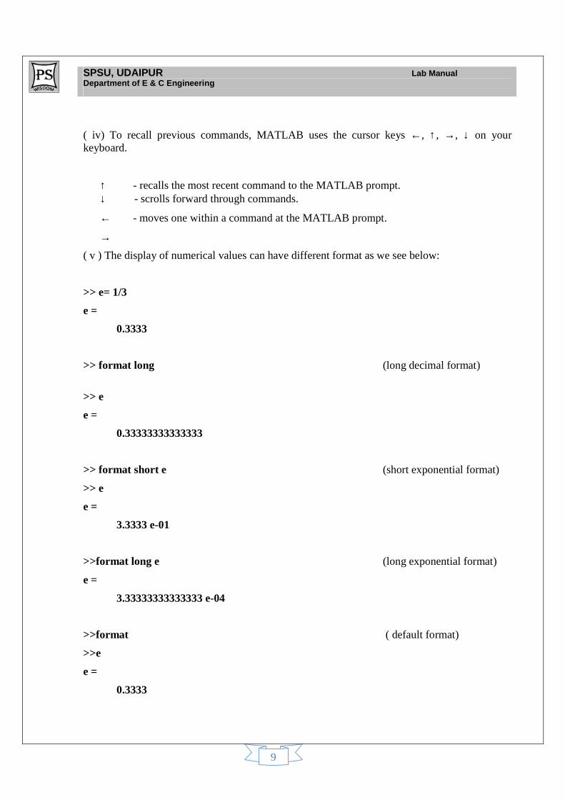
( v ) The display of numerical values can have different format as we see below:
>> e= 1/3
e =
0.3333
>> format long (long decimal format)
>> e
e =
0.33333333333333
>> format short e (short exponential format)
>> e
e =
3.3333 e-01
>>format long e (long exponential format)
e =
3.33333333333333 e-04
>>format ( default format)
>>e
e =
0.3333
SPSU, UDAIPUR Lab Manual Department of E & C Engineering
10
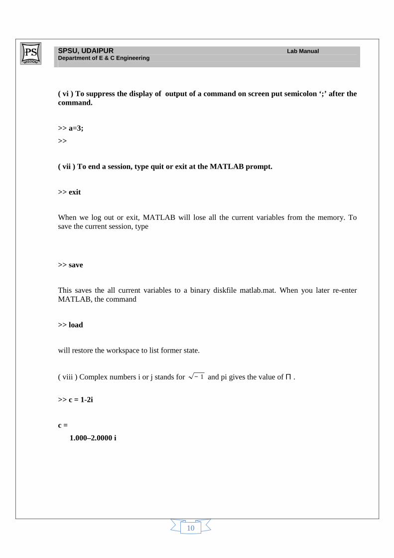
( vi ) To suppress the display of output of a command on screen put semicolon ‘;’ after the command.
>> a=3;
>>
( vii ) To end a session, type quit or exit at the MATLAB prompt.
>> exit
When we log out or exit, MATLAB will lose all the current variables from the memory. To save the current session, type
>> save
This saves the all current variables to a binary diskfile matlab.mat. When you later re-enter MATLAB, the command
>> load
will restore the workspace to list former state.
( viii ) Complex numbers i or j stands for 1− and pi gives the value of Π .
>> c = 1-2i
c =
1.000–2.0000 i
SPSU, UDAIPUR Lab Manual Department of E & C Engineering
11
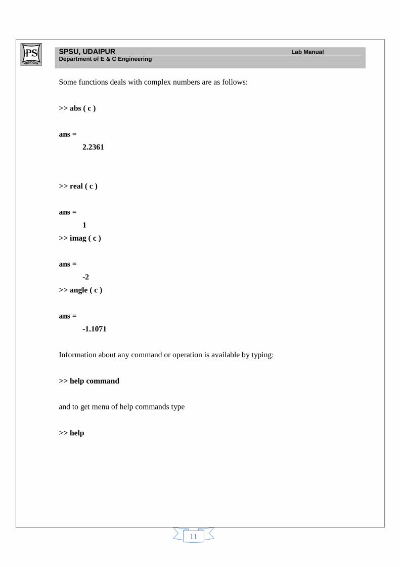
Some functions deals with complex numbers are as follows:
>> abs ( c )
ans =
2.2361
>> real ( c )
ans =
1
>> imag ( c )
ans =
-2
>> angle ( c )
ans =
-1.1071
Information about any command or operation is available by typing:
>> help command
and to get menu of help commands type
>> help
SPSU, UDAIPUR Lab Manual Department of E & C Engineering
12
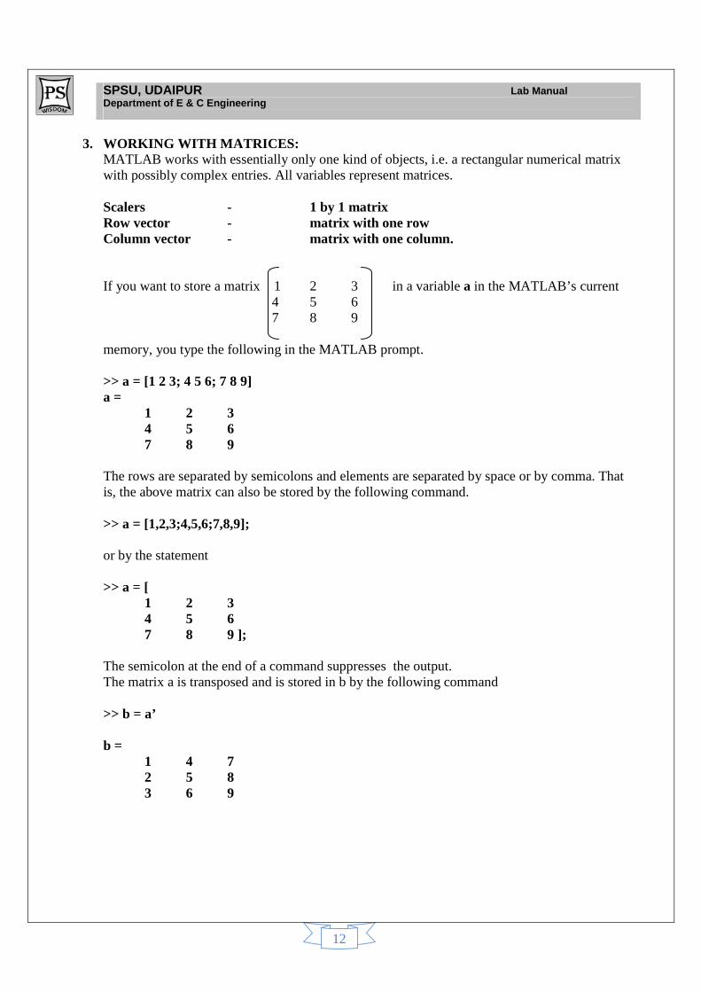
3. WORKING WITH MATRICES: MATLAB works with essentially only one kind of objects, i.e. a rectangular numerical matrix with possibly complex entries. All variables represent matrices. Scalers - 1 by 1 matrix Row vector - matrix with one row Column vector - matrix with one column. If you want to store a matrix 1 2 3 in a variable a in the MATLAB’s current 4 5 6 7 8 9 memory, you type the following in the MATLAB prompt. >> a = [1 2 3; 4 5 6; 7 8 9] a = 1 2 3 4 5 6 7 8 9 The rows are separated by semicolons and elements are separated by space or by comma. That is, the above matrix can also be stored by the following command. >> a = [1,2,3;4,5,6;7,8,9]; or by the statement >> a = [ 1 2 3 4 5 6 7 8 9 ]; The semicolon at the end of a command suppresses the output. The matrix a is transposed and is stored in b by the following command >> b = a’ b = 1 4 7 2 5 8 3 6 9
SPSU, UDAIPUR Lab Manual Department of E & C Engineering
13
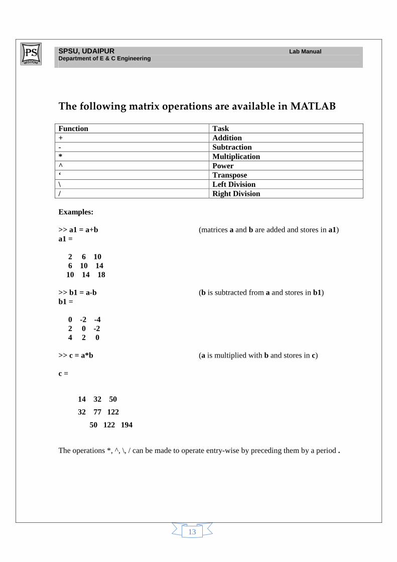
The following matrix operations are available in MATLAB Function Task + Addition - Subtraction * Multiplication ^ Power ‘ Transpose \ Left Division / Right Division Examples: >> a1 = a+b (matrices a and b are added and stores in a1) a1 = 2 6 10 6 10 14 10 14 18 >> b1 = a-b (b is subtracted from a and stores in b1) b1 = 0 -2 -4 2 0 -2 4 2 0 >> c = a*b (a is multiplied with b and stores in c) c =
14 32 50
32 77 122
50 122 194
The operations *, ^, \, / can be made to operate entry-wise by preceding them by a period .
SPSU, UDAIPUR Lab Manual Department of E & C Engineering
14
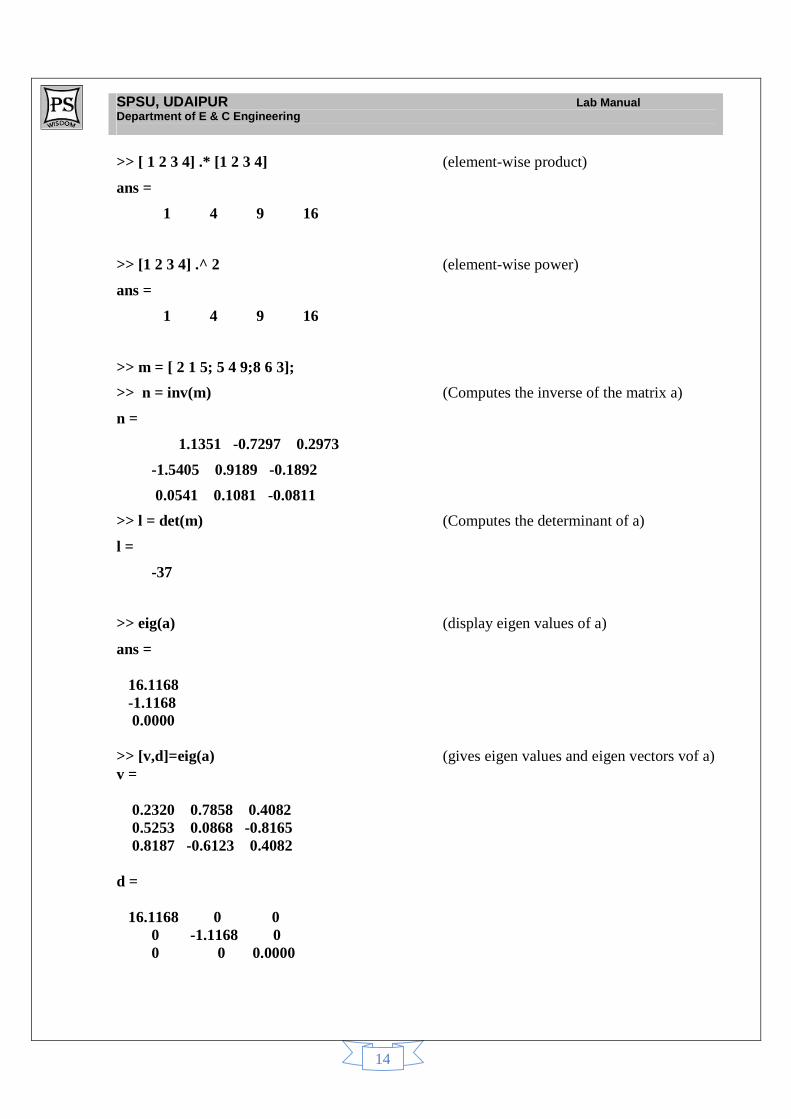
>> [ 1 2 3 4] .* [1 2 3 4] (element-wise product)
ans =
1 4 9 16
>> [1 2 3 4] .^ 2 (element-wise power)
ans =
1 4 9 16
>> m = [ 2 1 5; 5 4 9;8 6 3];
>> n = inv(m) (Computes the inverse of the matrix a)
n =
1.1351 -0.7297 0.2973
-1.5405 0.9189 -0.1892
0.0541 0.1081 -0.0811
>> l = det(m) (Computes the determinant of a)
l =
-37
>> eig(a) (display eigen values of a)
ans = 16.1168 -1.1168 0.0000 >> [v,d]=eig(a) (gives eigen values and eigen vectors vof a) v = 0.2320 0.7858 0.4082 0.5253 0.0868 -0.8165 0.8187 -0.6123 0.4082 d = 16.1168 0 0 0 -1.1168 0 0 0 0.0000
SPSU, UDAIPUR Lab Manual Department of E & C Engineering
15
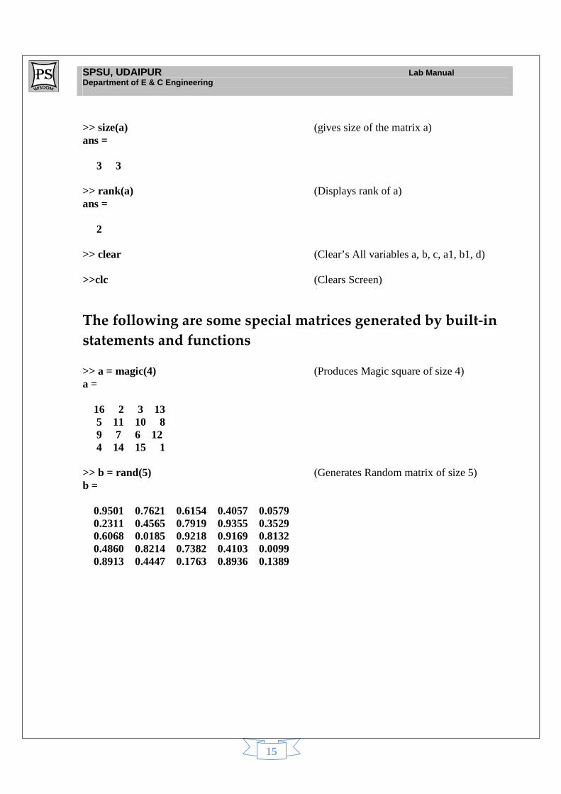
>> size(a) (gives size of the matrix a) ans =
3 3 >> rank(a) (Displays rank of a) ans = 2 >> clear (Clear’s All variables a, b, c, a1, b1, d) >>clc (Clears Screen)
The following are some special matrices generated by built-in
statements and functions >> a = magic(4) (Produces Magic square of size 4) a = 16 2 3 13 5 11 10 8 9 7 6 12 4 14 15 1 >> b = rand(5) (Generates Random matrix of size 5) b = 0.9501 0.7621 0.6154 0.4057 0.0579 0.2311 0.4565 0.7919 0.9355 0.3529 0.6068 0.0185 0.9218 0.9169 0.8132 0.4860 0.8214 0.7382 0.4103 0.0099 0.8913 0.4447 0.1763 0.8936 0.1389
SPSU, UDAIPUR Lab Manual Department of E & C Engineering
16
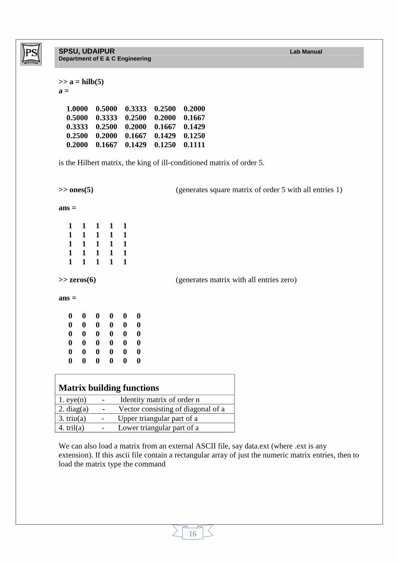
>> a = hilb(5) a = 1.0000 0.5000 0.3333 0.2500 0.2000 0.5000 0.3333 0.2500 0.2000 0.1667 0.3333 0.2500 0.2000 0.1667 0.1429 0.2500 0.2000 0.1667 0.1429 0.1250 0.2000 0.1667 0.1429 0.1250 0.1111 is the Hilbert matrix, the king of ill-conditioned matrix of order 5. >> ones(5) (generates square matrix of order 5 with all entries 1) ans = 1 1 1 1 1 1 1 1 1 1 1 1 1 1 1 1 1 1 1 1 1 1 1 1 1 >> zeros(6) (generates matrix with all entries zero) ans = 0 0 0 0 0 0 0 0 0 0 0 0 0 0 0 0 0 0 0 0 0 0 0 0 0 0 0 0 0 0 0 0 0 0 0 0
Matrix building functions 1. eye(n) - Identity matrix of order n 2. diag(a) - Vector consisting of diagonal of a 3. triu(a) - Upper triangular part of a 4. tril(a) - Lower triangular part of a We can also load a matrix from an external ASCII file, say data.ext (where .ext is any extension). If this ascii file contain a rectangular array of just the numeric matrix entries, then to load the matrix type the command
SPSU, UDAIPUR Lab Manual Department of E & C Engineering
17
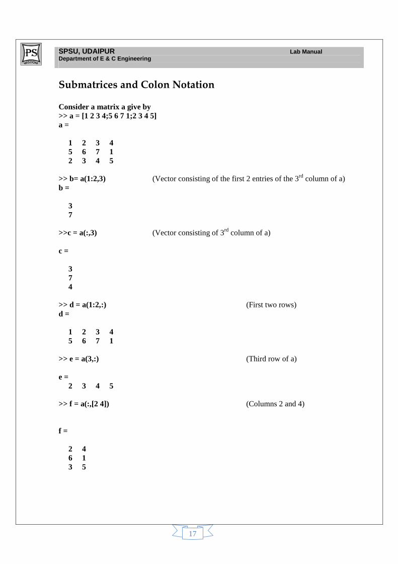
Submatrices and Colon Notation Consider a matrix a give by >> a = [1 2 3 4;5 6 7 1;2 3 4 5] a = 1 2 3 4 5 6 7 1 2 3 4 5 >> b= a(1:2,3) (Vector consisting of the first 2 entries of the 3rd column of a) b = 3 7 >>c = a(:,3) (Vector consisting of 3rd column of a) c = 3 7 4 >> d = a(1:2,:) (First two rows) d = 1 2 3 4 5 6 7 1 >> e = a(3,:) (Third row of a) e = 2 3 4 5 >> f = a(:,[2 4]) (Columns 2 and 4) f = 2 4 6 1
3 5
SPSU, UDAIPUR Lab Manual Department of E & C Engineering
18
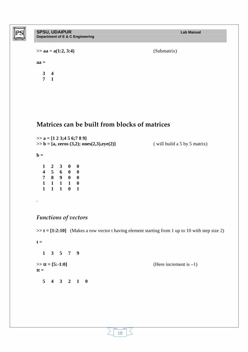
>> aa = a(1:2, 3:4) (Submatrix) aa = 3 4
7 1
Matrices can be built from blocks of matrices >> a = [1 2 3;4 5 6;7 8 9] >> b = [a, zeros (3,2); ones(2,3),eye(2)] ( will build a 5 by 5 matrix) b = 1 2 3 0 0 4 5 6 0 0 7 8 9 0 0 1 1 1 1 0 1 1 1 0 1 .
Functions of vectors >> t = [1:2:10] (Makes a row vector t having element starting from 1 up to 10 with step size 2) t = 1 3 5 7 9 >> tt = [5:-1:0] (Here increment is –1) tt = 5 4 3 2 1 0
SPSU, UDAIPUR Lab Manual Department of E & C Engineering
19
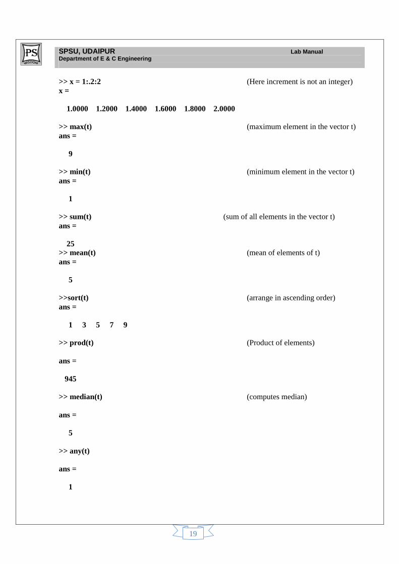
>> x = 1:.2:2 (Here increment is not an integer) x = 1.0000 1.2000 1.4000 1.6000 1.8000 2.0000 >> max(t) (maximum element in the vector t) ans = 9 >> min(t) (minimum element in the vector t) ans = 1 >> sum(t) (sum of all elements in the vector t) ans = 25 >> mean(t) (mean of elements of t) ans = 5 >>sort(t) (arrange in ascending order) ans = 1 3 5 7 9 >> prod(t) (Product of elements) ans = 945 >> median(t) (computes median) ans = 5 >> any(t) ans = 1
SPSU, UDAIPUR Lab Manual Department of E & C Engineering
20
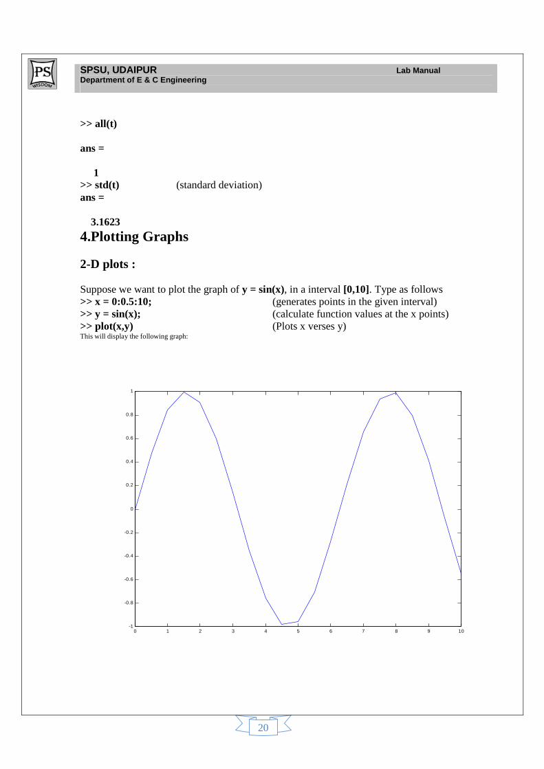
>> all(t) ans = 1 >> std(t) (standard deviation) ans = 3.1623
4.Plotting Graphs 2-D plots : Suppose we want to plot the graph of y = sin(x), in a interval [0,10]. Type as follows >> x = 0:0.5:10; (generates points in the given interval) >> y = sin(x); (calculate function values at the x points) >> plot(x,y) (Plots x verses y) This will display the following graph:
0 1 2 3 4 5 6 7 8 9 10-1
-0.8
-0.6
-0.4
-0.2
0
0.2
0.4
0.6
0.8
1
SPSU, UDAIPUR Lab Manual Department of E & C Engineering
21
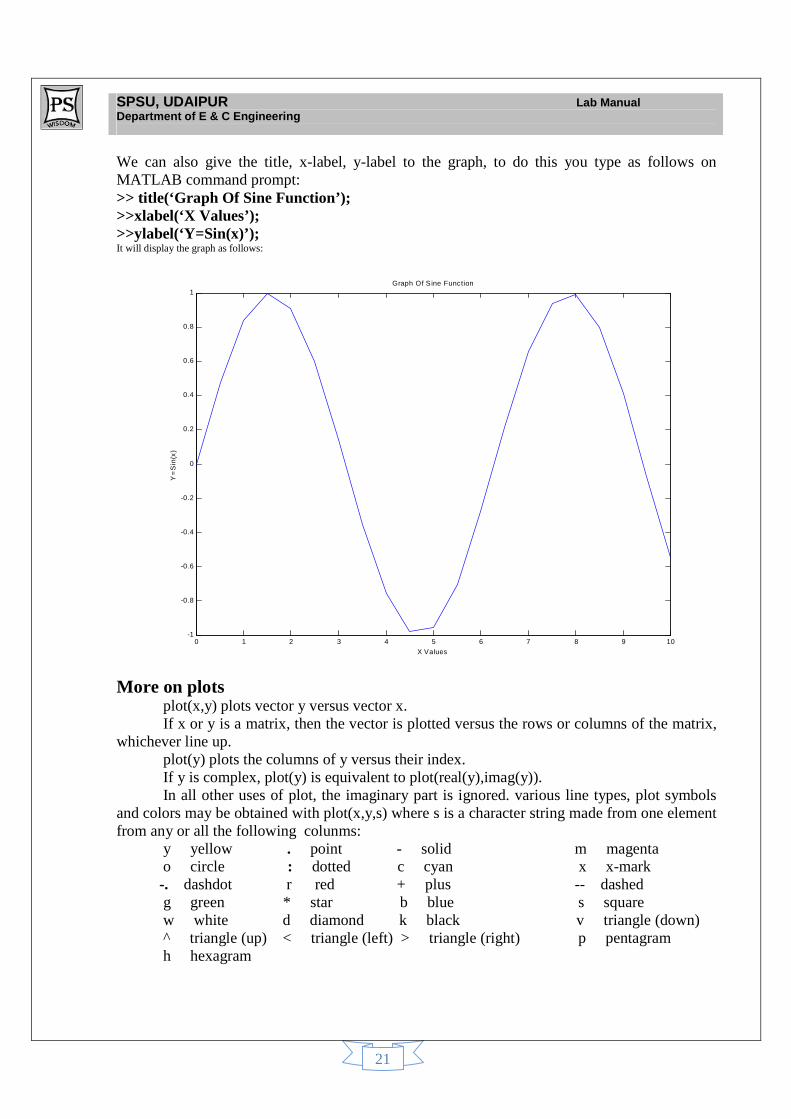
We can also give the title, x-label, y-label to the graph, to do this you type as follows on MATLAB command prompt: >> title(‘Graph Of Sine Function’); >>xlabel(‘X Values’); >>ylabel(‘Y=Sin(x)’); It will display the graph as follows:
0 1 2 3 4 5 6 7 8 9 10-1
-0.8
-0.6
-0.4
-0.2
0
0.2
0.4
0.6
0.8
1Graph Of S ine Function
X Values
Y=
Sin
(x)
More on plots plot(x,y) plots vector y versus vector x.
If x or y is a matrix, then the vector is plotted versus the rows or columns of the matrix, whichever line up. plot(y) plots the columns of y versus their index.
If y is complex, plot(y) is equivalent to plot(real(y),imag(y)). In all other uses of plot, the imaginary part is ignored. various line types, plot symbols and colors may be obtained with plot(x,y,s) where s is a character string made from one element from any or all the following colunms: y yellow . point - solid m magenta o circle : dotted c cyan x x-mark -. dashdot r red + plus -- dashed g green * star b blue s square w white d diamond k black v triangle (down) ^ triangle (up) < triangle (left) > triangle (right) p pentagram h hexagram
SPSU, UDAIPUR Lab Manual Department of E & C Engineering
22
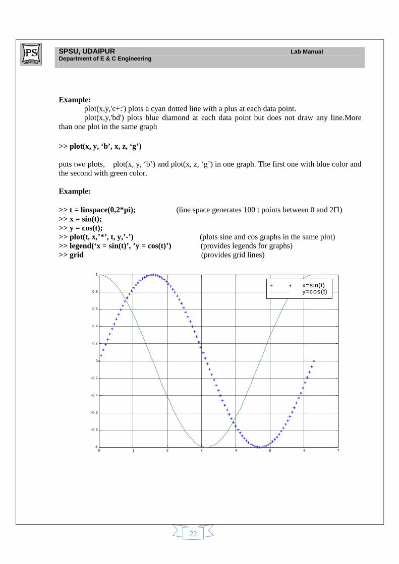
Example: plot(x,y,'c+:') plots a cyan dotted line with a plus at each data point. plot(x,y,'bd') plots blue diamond at each data point but does not draw any line.More than one plot in the same graph >> plot(x, y, ‘b’, x, z, ‘g’) puts two plots, plot(x, y, ‘b’) and plot(x, z, ‘g’) in one graph. The first one with blue color and the second with green color. Example: >> t = linspace(0,2*pi); (line space generates 100 t points between 0 and 2Π) >> x = sin(t); >> y = cos(t); >> plot(t, x,’*’, t, y,’-’) (plots sine and cos graphs in the same plot) >> legend(‘x = sin(t)’, ’y = cos(t)’) (provides legends for graphs) >> grid (provides grid lines)
0 1 2 3 4 5 6 7-1
-0.8
-0.6
-0.4
-0.2
0
0.2
0.4
0.6
0.8
1
x=sin(t)y=cos(t)
SPSU, UDAIPUR Lab Manual Department of E & C Engineering
23
plot(x1,y1,s1,x2,y2,s2,x3,y3,s3,...) combines the plots defined by the (x,y,s) triples, where the x's and y's are vectors or matrices and the s's are strings. plot(x,y,'y-',x,y,'go') plots the data twice, with a solid yellow line interpolating green circles at the data points.
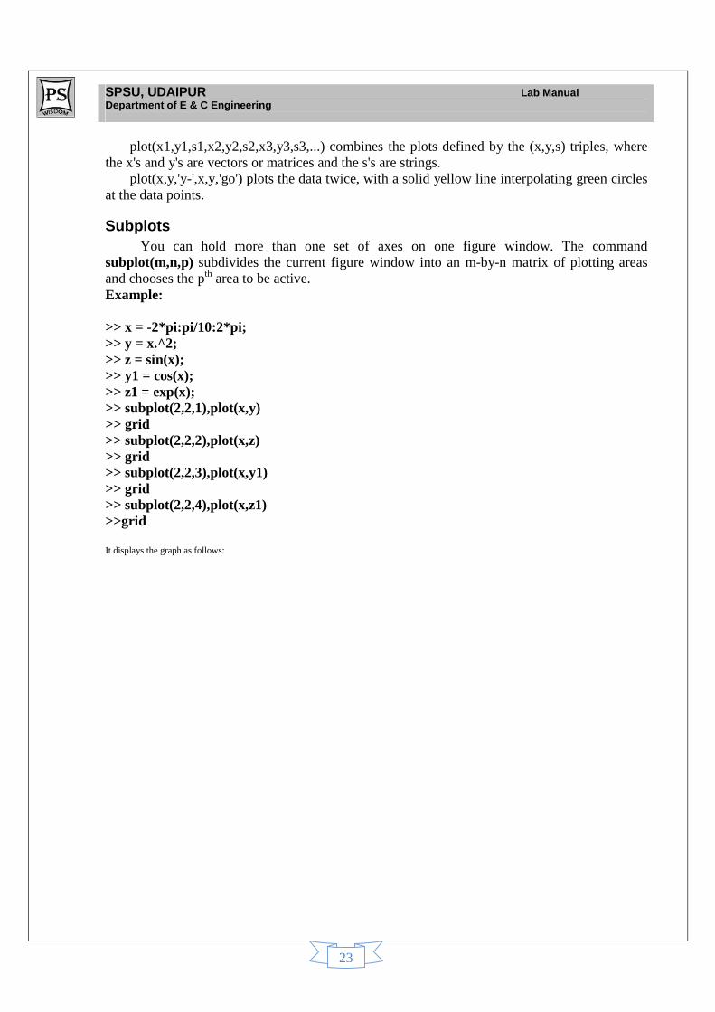
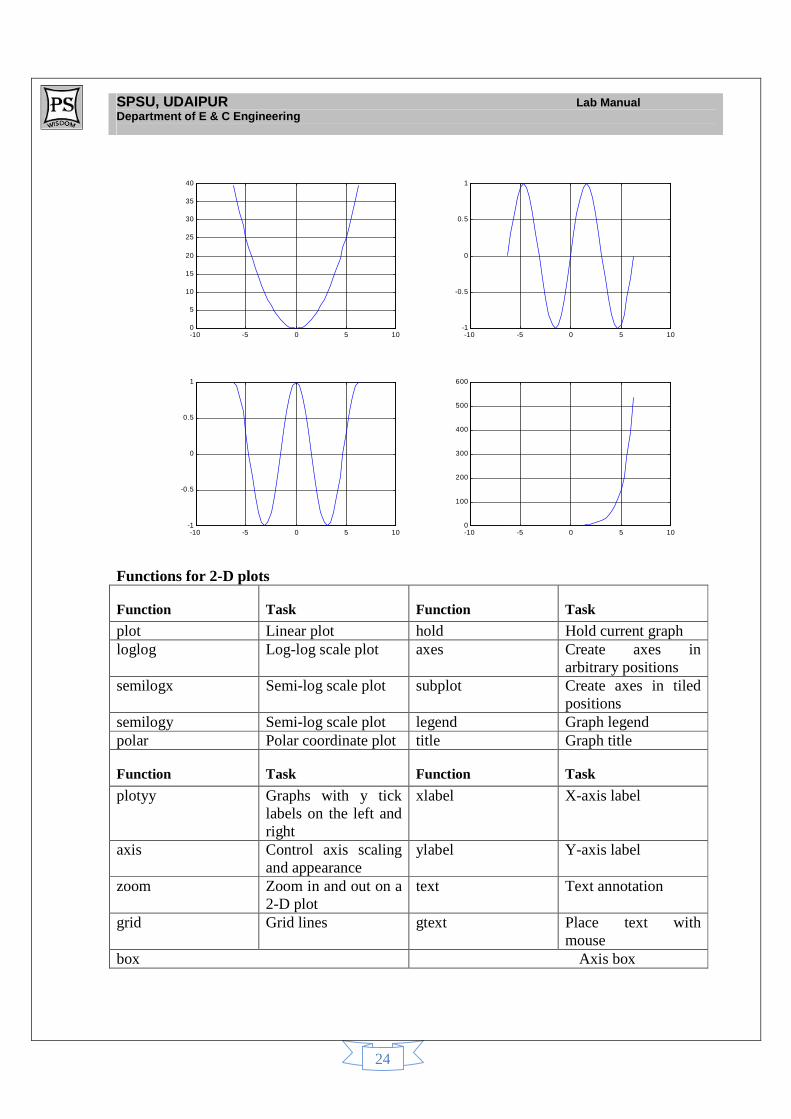
Subplots You can hold more than one set of axes on one figure window. The command subplot(m,n,p) subdivides the current figure window into an m-by-n matrix of plotting areas and chooses the pth area to be active. Example: >> x = -2*pi:pi/10:2*pi; >> y = x.^2; >> z = sin(x); >> y1 = cos(x); >> z1 = exp(x); >> subplot(2,2,1),plot(x,y) >> grid >> subplot(2,2,2),plot(x,z) >> grid >> subplot(2,2,3),plot(x,y1) >> grid >> subplot(2,2,4),plot(x,z1) >>grid It displays the graph as follows:
SPSU, UDAIPUR Lab Manual Department of E & C Engineering
24
-10 -5 0 5 100
5
10
15
20
25
30
35
40
-10 -5 0 5 10-1
-0.5
0
0.5
1
-10 -5 0 5 10-1
-0.5
0
0.5
1
-10 -5 0 5 100
100
200
300
400
500
600
Functions for 2-D plots
Function Task Function Task
plot Linear plot hold Hold current graph loglog Log-log scale plot axes Create axes in
arbitrary positions semilogx Semi-log scale plot subplot Create axes in tiled
positions semilogy Semi-log scale plot legend Graph legend polar Polar coordinate plot title Graph title
Function Task Function Task
plotyy Graphs with y tick labels on the left and right
xlabel X-axis label
axis Control axis scaling and appearance
ylabel Y-axis label
zoom Zoom in and out on a 2-D plot
text Text annotation
grid Grid lines gtext Place text with mouse
box Axis box
SPSU, UDAIPUR Lab Manual Department of E & C Engineering
25
MATLAB Programming
We can also do programming in MATLAB as we are doing in FORTRAN, C & C++. To make a file in MATLAB we have to click on “New” in the file menu in menubar. It will open a new file as we are doing in “word”; and if we save this file (called m-file), will be saved in “bin” folder of MATLAB. Such files are called “M-files” because they have an extension of “.m” in its filename. Much of your work with MATLAB will be creating and refining M-files. There are two types of M-files: Script Files and Function Files
Script Files A script file consists of a sequence of normal MATLAB statements. If the file has the filename, say, rkg.m, then the MATLAB command >> rkg will cause the statements in the file to be executed. Variables in a script file are global and will change the value of variables of the same name in the environment of the current MATLAB session. Script files are often used to enter data into a large matrix; in such a file, entry errors can be easily edited out. Example: In a file rkg.m enter the following: % This is a sample m-file a = [1,2,3;0,1,1;1,2,3] b =a’; c = a+b d = inv(c) save this file. Then to execute this file, type >> rkg <ENTER> a = 1 2 3 0 1 1 1 2 3 b = 1 0 1 2 1 2 3 1 3
SPSU, UDAIPUR Lab Manual Department of E & C Engineering
26
c = 2 2 4 2 2 3 4 3 6 d = -1.5000 0 1.0000 0 2.0000 -1.0000 1.0000 -1.0000 0 The % symbol indicates that the rest of the line is a comments. MATLAB will ignore the rest of the line. However, the first comment lines which document the m-file are available to the on-line help facility and will be displayed A M-file can also reference other M-files, including referencing itself recursively.
Function Files Function files provide extensibility to MATLAB. You can create new functions specific to your problem which will then have the same status as other MATLAB functions. Variables in a function file are by default local. However, you can declare a variable to be global if you wish.
Example function y = prod (a,b) y = a*b; Save this file with filename prod.m then type on the MATLAB prompt >> prod (3,4) ans = 12 In MATLAB to get input from user the syntax rule is : variable name = input (‘variable’); As we know that if we don’t write “;” after a statement in MATLAB, it will print the output also. That means if in a programme we write: a=input (‘ Enter a number ‘);
SPSU, UDAIPUR Lab Manual Department of E & C Engineering
27
And on command prompt if we run this program it will be displayed like: >> Enter a number If we type 2 at the cursor then we get the output as a=2
Control Flow
MATLAB offers the following decision making or control flow structures:
1. If- Else –End Construction 2. For loops 3. While loops 4. Switch-Case constructions etc.
SYNTAX RULE FOR CONTROLLING THE FLOW: 1) if statement condition: The general form of the if statement is:
if expression statements elseif expression statements else statements end The statements are executed if the real part of the expression has all non-zero elements. The else and elseif parts are optional. zero or more elseif parts can be used as well as nested if's. The expression is usually of the form expr rop expr where rop is ==, <, >, <=, >=, or ~=. Example: if i == j a(i,j) = 2; elseif abs(i-j) == 1 a(i,j) = -1; else
SPSU, UDAIPUR Lab Manual Department of E & C Engineering
28
2) else used with if : else is used with if . The statements after the else are executed if all the preceeding if and elseif expressions are false. The general form of the if statement is: if expression statements elseif expression statements else statements end 3) elseif if statement condition: elseif is used with if. The statements after the elseif are executed if the expression is true and all the preceeding if and elseif expressions are false. An expression is considered true if the real part has all non-zero elements. elseif does not need a matching end, while else if does. the general form of the if statement is: if expression statements elseif expression statements else statements end 4) end terminate scope of for, while, switch, try, and if statements. Without end's, for, while, switch, try, and if wait for further input. each end is paired with the closest previous unpaired for, while, switch, try or if and serves to terminate its scope. end can also serve as the last index in an indexing expression. in that context, end = size(x,k) when used as part of the k-th index. examples of this use are, x(3:end) and x(1,1:2:end-1). when using end to grow an array, as in x(end+1) = 5, make sure x exists first. 5) for repeat statements a specific number of times: The general form of a for statement is: for variable = expr, statement, ..., statement end The columns of the expression are stored one at a time in the variable and then the following statements, up to the end, are executed. The expression is often of the form x:y, in which case its columns are simply scalars. some examples Example: (assume n has already been assigned a value) for i = 1:n, for j = 1:n, a(i,j) = 1/(i+j-1); end end
SPSU, UDAIPUR Lab Manual Department of E & C Engineering
29
for s = 1.0: -0.1: 0.0, end steps s with increments of -0.1 for e = eye(n), ... end sets e to the unit n-vectors. Long loops are more memory efficient when the colon expression appears in the for statement since the index vector is never created.
6) The break statement can be used to terminate the loop prematurely. break terminate execution of while or for loop. In nested loops, break exits from the innermost loop only. 7) while repeat statements an indefinite number of times. The general form of a while statement is:
while expression statements end The statements are executed while the real part of the expression has all non-zero elements. The expression is usually the result of expr rop expr where rop is ==, <, >, <=, >=, or ~=. Example:
(assuming a already defined) e = 0*a; f = e + eye(size(e)); n = 1; while norm(e+f-e,1) > 0, e = e + f; f = a*f/n; n = n + 1; end 8) switch switches among several cases based on expression: the general form of the switch statement is: switch switch_expr case case_expr, statement, ..., statement case {case_expr1, case_expr2, case_expr3,...} statement, ..., statement ... otherwise, statement, ..., statement end The first case where the switch_expr matches the case_expr is executed. when the case expression is a cell array (as in the second case above), the case_expr matches if any of the elements of the cell array match the switch expression. If none of the case expressions match the switch expression then the otherwise case is executed (if it exists). Only one case is
SPSU, UDAIPUR Lab Manual Department of E & C Engineering
30
executed and execution resumes with the statement after the end. the switch_expr can be a scalar or a string. A scalar switch_expr matches a case_expr if switch_expr==case_expr. A string switch_expr matches a case_expr if strcmp(switch_expr,case_expr) returns 1 (true). Example: (assuming method exists as a string variable): switch lower(method) case {'linear','bilinear'}, disp('method is linear') case 'cubic', disp('method is cubic') case 'nearest', disp('method is nearest') otherwise, disp('unknown method.') end 9) case switch statement case: case is part of the switch statement syntax, whose general form is: switch switch_expr case case_expr, statement, ..., statement case {case_expr1, case_expr2, case_expr3,...} statement, ..., statement ... otherwise, statement, ..., statement end 10) otherwise default switch statement case. otherwise is part of the switch statement syntax, whose general form is: switch switch_expr case case_expr, statement, ..., statement case {case_expr1, case_expr2, case_expr3,...} statement, ..., statement ... otherwise, statement, ..., statement end The otherwise part is executed only if none of the preceeding case expressions match the switch expression.
SPSU, UDAIPUR Lab Manual Department of E & C Engineering
31
11) try begin try block: The general form of a try statement is: try, statement, ..., statement, catch, statement, ..., statement end Normally, only the statements between the try and catch are executed. however, if an error occurs while executing any of the statements, the error is captured into lasterr and the statements between the catch and end are executed. if an error occurs within the catch statements, execution will stop unless caught by another try...catch block. The error string produced by a failed try block can be obtained with lasterr. 12) catch begin catch block: The general form of a try statement is: try statement, ..., statement, catch statement, ..., statement end 13) return returns to invoking function: return causes a return to the invoking function or to the keyboard. it also terminates the keyboard mode. normally functions return when the end of the function is reached. a return statement can be used to force an early return. Example: function d = det(a) if isempty(a) d = 1; return else ... end How to run a program in MATLAB? Suppose we have created a m-file & saved. Now to run this program, on command prompt type the file name and just press the ENTER KEY that will run the file. Data File:
SPSU, UDAIPUR Lab Manual Department of E & C Engineering
32
Now to make a data file in MATLAB, we just make a file in which all the data are stored. Now we make another file in which the operation on that data is to be done. Then in this file, where we have to call that data we have to just type the file name of the file in which data is stored and write the rest of the programming statements. So when run this file the file in which data is stored will be called and then rest of the programming statements are executed & finally we get the output. MEX-Files: We can call our C programs from MATLAB as if they were built in functions. Those programs in C which are callable in MATLAB are referred as MEX-Files. MEX-files are dynamically linked subroutines that the MATLAB interpreter can automatically load & execute. For example the following program in C to add two integers having file name “add”. #include<stdio.h> main( ) { int a=2,b=3; d=a+b; printf(‘sum is:’,d); return 0; } To compile & link this example at the MATLAB prompt, type >>mex add.c and press the “ENTER”key, it will give the output. Some useful commands for programming: >> echo on --- Echoing of commands in all script files >> echo off --- Turns off echo >> echo on all --- turns on of command including function files >> disp(‘Any string’) --- Displays the string
>> diary file --- Causes copy of all subsequent keyboard input and most of the resulting output (but not graphs) to be written on the named file.
>> pause --- causes to stop execution of until any key is pressed. Some Examples:
1) Example for if, else
for i = 1:n for j = 1:n if i==j a(i, j) = 2
SPSU, UDAIPUR Lab Manual Department of E & C Engineering
33
elseif abs(i – j) ==1 a(i, j) = -1; else a(i, j) = 0; end end end 2) Example for while eps = 1 while (1+eps)>1 eps = eps/2; end eps = eps*2 3) Gauss Elimination Method function [x] = gausselim(A,b)
% This subroutine will perform Gaussian elimination on the matrix you pass and solve % the system AX = b
N = max(size(A)) for j = 2:N for i = j:N m = A(j,j-1) / A(j-1,j-1); A(i, :) = A(i, :) – A(j-1,:)*m; b(i) = b(i) – m*b(j-1); end end %Perform back substitution x = zeros(N, 1) x(N) = b(N) / A(N, N) for j = N-1:-1:1
x(j) = (b(j)-A(j,j+1:N)) / A(j, j) end
SPSU, UDAIPUR Lab Manual Department of E & C Engineering
34
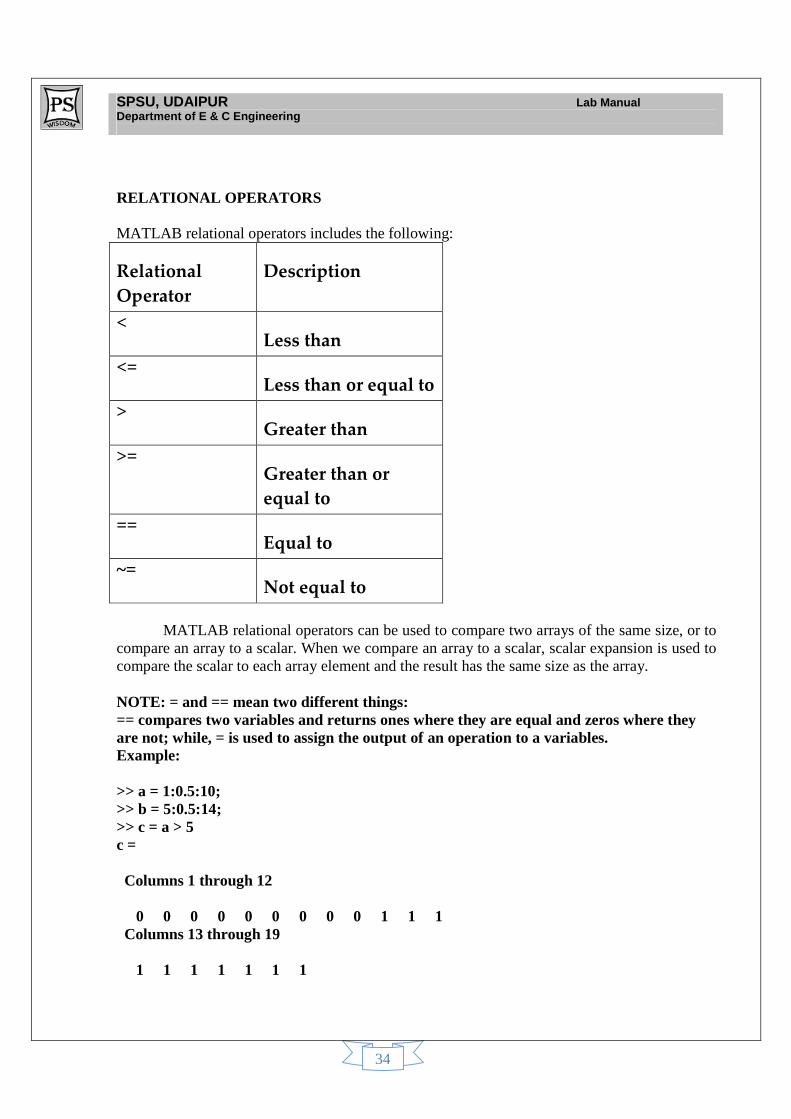
RELATIONAL OPERATORS MATLAB relational operators includes the following:
Relational
Operator
Description
< Less than
<= Less than or equal to
> Greater than
>= Greater than or
equal to
== Equal to
~= Not equal to
MATLAB relational operators can be used to compare two arrays of the same size, or to compare an array to a scalar. When we compare an array to a scalar, scalar expansion is used to compare the scalar to each array element and the result has the same size as the array. NOTE: = and == mean two different things: == compares two variables and returns ones where they are equal and zeros where they are not; while, = is used to assign the output of an operation to a variables. Example: >> a = 1:0.5:10; >> b = 5:0.5:14; >> c = a > 5 c = Columns 1 through 12 0 0 0 0 0 0 0 0 0 1 1 1 Columns 13 through 19 1 1 1 1 1 1 1
SPSU, UDAIPUR Lab Manual Department of E & C Engineering
35
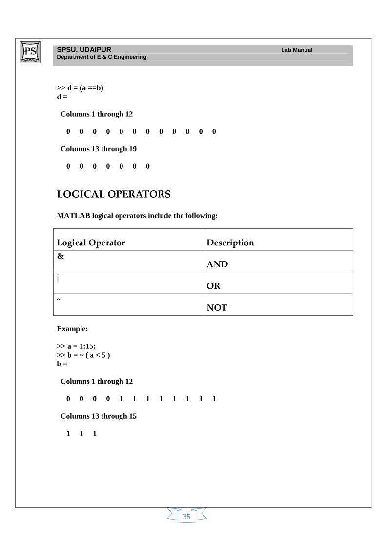
>> d = (a ==b) d = Columns 1 through 12 0 0 0 0 0 0 0 0 0 0 0 0 Columns 13 through 19 0 0 0 0 0 0 0
LOGICAL OPERATORS MATLAB logical operators include the following:
Logical Operator Description
& AND
| OR
~ NOT
Example: >> a = 1:15; >> b = ~ ( a < 5 ) b = Columns 1 through 12 0 0 0 0 1 1 1 1 1 1 1 1 Columns 13 through 15 1 1 1
SPSU, UDAIPUR Lab Manual Department of E & C Engineering
36
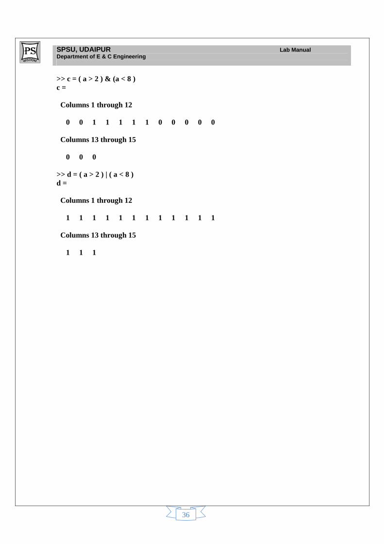
>> c = ( a > 2 ) & (a < 8 ) c = Columns 1 through 12 0 0 1 1 1 1 1 0 0 0 0 0 Columns 13 through 15 0 0 0 >> d = ( a > 2 ) | ( a < 8 ) d = Columns 1 through 12 1 1 1 1 1 1 1 1 1 1 1 1 Columns 13 through 15 1 1 1
SPSU, UDAIPUR Lab Manual Department of E & C Engineering
37
RULES FOR CONSTRUCTING M-FILES Function M-files must satisfy a number of criteria. Some of them are as follows:
1. The function M-file name and the function name ( e.g., rkg) that appears in the first line of the file should be identical. In reality, MATLAB ignores the function name in the first line and executes functions based on the file name stored on disk.
2. Function M-file names can have up to 31 characters. This maximum may be limited by the operating system, in which case the lower limit applies. MATLAB ignores characters beyond the thirty-first or the operating system limit, so longer names can be used, provided the legal characters point to a unique file name.
3. Function names must begin with a letter. Any combination of letters, numbers, and underscores can appear after the first character. This naming rule is identical to that for variables.
4. The first line of a function M-file is called the function declaration line and must contain the word function followed by the calling syntax for the function in its most general form. The input and output variables identified in the first line are variables local to the function. The input variables contain data passed to the function and the output variables contain data passed back from the function. It is not possible to pass data back though the input variables.
5. The first sets of contiguous comment lines after the function declaration line are the help text for the function. The first comment line is called the H1 line and is the line searched by the lookfor command. The H1 line typically contains the function name in uppercase characters and a concise description of the function’s purpose. Comment lines after the first describe possible calling syntaxes, algorithms used, and simple examples, if appropriate.
6. All statements after the first set of contiguous comment lines compose the body of the function. The body of a function contains MATLAB statements that operate on the input arguments and produce results in the output arguments.
7. A function M-file terminates after the last line in the file is executed or whenever a return statement is encountered.
8. A function can abort operation and return control to the command window by calling the function error. This function is useful for flagging improper function usage, as shown in the following file fragment: if length ( mat ) > 1 error ( ‘MAT must be a scalar.’) end
if the function error is executed as shown, the string ‘VAL must be a scalar.’ Is displayed in the command window after a line identifying the file the error message originated from. If the function error is given a zero-length character string, it takes no action.
SPSU, UDAIPUR Lab Manual Department of E & C Engineering
38
9. A function can report a warning and then continue operation by calling the function warning. This function is useful for reporting exceptions and other anomalous behavior. warning (‘some message’) displays a character string in the command window. The difference between the function warning and the function disp is that warning messages can be turned on or off globally by issuing the commands warning on and warning off , respectively.
10. Function M-files can contain calls to script files. When a script file is encountered, it is evaluated in the function’s workspace, not the MATLAB workspace.
11. Multiple functions can appear in a single function M-file. Additional functions, called subfunctions or local functions, are simply appended to the end of the primary function. Subfunctions begin with a standard function statement line and follow function construction rules.
12. Subfunctions can be called by the primary function in the M-file as well as by other subfunctions in the same M-file. As with all functions, subfunctions have their own individual workspaces.
13. Subfunctions can appear in any order after the primary function in a M-file. Help text for subfunctions is not returned by the help command.
14. It is suggested that subfunction names begin with the word local (e.g., local_bsr). Doing so improves the readability of the primary function because calls to local functions are clearly identifiable. All local function names can have up to 31 characters.
15. In addition to subfunctions, M-files can call private M-files, which are standard function M-files that reside in a subdirectory of the calling function that is entitled private. Only functions in the immediate parent directory of private M-files have access to private M-file.
16. It is suggested that private M-file names begin with the word private (e.g., private_bsr). Doing so improve the readability of the primary function because calls to private functions are clearly identifiable. As with other function names, all private M-file names can have up to 31 characters.
INPUT AND OUTPUT ARGUMENTS MATLAB functions can have any number of input and output arguments. The features and criteria of these arguments are as follows:
1. Function M-files can have zero input and zero output arguments. 2. Functions can be called with fewer input and output arguments than the function
definition line in the M-file specifies. Functions cannot be called with more input or output arguments than the M-file specifies.
3. The number of input and output arguments used in a function call can be determined by calls to the functions nargin and nargout, respectively. Since nargin and nargout are functions, not variables, one cannot reassign them with statements such as
Nargin = nargin – 1
SPSU, UDAIPUR Lab Manual Department of E & C Engineering
39
4. When a function is called, the input variables are not copied into the function’s workspace, but their values are made readable within the function. However, if any values in the input variables are changed, the array is then copied into the function’s workspace. Thus, to conserve memory and increase speed, it is best to extract elements from large arrays and then modify them, rather than forcing the entire array to be copied into the function’s workspace. Note that using the same variable name for both an input and output argument causes an immediate copying of the contents of the variable into the function’s workspace. For example,
function y = myfunction (x, y, z) causes the variable y to be copied immediately into the workspace of myfunction.
5. If a function declares one or more output arguments, but no output is desired, simply do not assign values to the output variable or variables.
6. Functions can accept a variable and unlimited number of input arguments by specifying varargin as the last input argument in the function declaration line. Varargin is a predefined cell array whose ith cell is the ith argument starting from where varargin appears. For example, consider a function having the function declaration line Function a = myfunction(varargin) If this function is called as a = myfunction(x, y, z), then inside the function varargin(1) contains the array x, varargin(2) contains the array y, and varargin(3) contains the array z. Likewise, if the function is called as a = myfunction(x), varargin has length 1 and varargin{1} = x. Every time myfunction is called, it can be called with a different number of arguments. In any case, the function nargin returns the actual number of input arguments used. In those cases where one or more input arguments are fixed, varargin must appear as the last argument, such as Function a = myfunction (x, y, varargin) If this function is called as a = myfunction(x, y, z), then inside the function x and y are available and varargin(1) contains z.
7. Functions can accept a variable and unlimited number of output arguments by specifying varargout as the last output argument in the function declaration line. Varargout is a predefined cell array whose ith cell is the ith argument starting from where varargout appears. For example, consider a function having the function declaration line
function varargout = myfunction (x) If this function is called as [a, b] = function (x), then inside the function the contents of varargout(1) must be assigned to the data that become the variable a, and varargout(2) must be assigned to the data that become the variable b. As with varargin , the length of varargout is equal to the number of output arguments used and nargout returns this length. In those cases where one or more output arguments are fixed, varargout must appear as the last argument in the function declaration line –for example, function [a, b, varargout] = myfunction (x).
SPSU, UDAIPUR Lab Manual Department of E & C Engineering
40
FUNCTION WORKSPACES Functions accept inputs, act on those inputs, and create outputs. Any and all variables created within the function are hidden from the MATLAB or base workspace. Each function has its own temporary workspace that is created with each function call and then deleted when the function completes execution. MATLAB functions can be called recursively and each call has a separate workspace. In addition to input and output arguments, MATLAB provides several techniques for communicating among function workspaces and the MATLAB or base workspace.
1. Function can share variables with other function, the MATLAB workspace, and recursive calls to themselves if the variables are declared global. To gain access to a global variable within a function or the MATLAB workspace, the variable must be declared global within each desired workspace. The MATLAB functions tic and toc illustrate the use of global variables. The functions tic and toc form a simple stopwatch for timing MATLAB operations. When tic is called, it declares the variable TICTOC global, assigns the current time to it, and then terminates. Later when toc is called, TICTOC is declared global in the toc workspace, there by providing access to its contents, and the elapsed time is computed. It is important to note that the variable TICTOC exists only in the workspaces of the functions tic and toc; it does not exist in the MATLAB workspace unless global TICTOC is issued there.
2. In addition to sharing data through global variables, MATLAB provides the function evalin, which allows one to reach into another workspace, evaluate an expression, and return the result to the current workspace. The function evalin is similar to eval, except that the string is evaluated in either the caller or base workspace. The caller workspace is the workspace from which the current function was called. The base workspace is the MATLAB workspace in the command window. For example, A = evalin(‘caller’,’expression’) evaluates ‘expression’ in the caller workspace and returns the results to the variable A in the current workspace. evalin also provides error trapping with the syntax evalin(‘workspace’,’try’,’catch’) , where ‘workspace’ is either ‘caller’ or ‘base’, ‘try’ is the first expression evaluated, and ‘catch’ is an expression that is evaluated in the current workspace if the evaluation of ‘try’ produces an error.
3. Since one can evaluate an expression in another workspace, it makes sense that one can also assign the results of some expression in the current workspace to a variable in another workspace. The function assignin provides this capability. assignin(‘workspace’,’vname’,X), where ‘workspace’ is either ‘caller’ or ‘base’, assigns the contents of the variable X in the current workspace to a variable in the ‘caller’ or ‘base’ workspace named ‘vname’.
4. The function inputname provides a way to determine the variable names used when a function is called. For example, suppose a function is called as >> y = myfunction(xdot,time,sqrt(2)) issuing inputname(1) inside of myfunction returns the character string ‘xdot’, inputname(2) returns ‘time’, and inputname (3) returns an empty array because sqrt(2) is not a variable, but rather an expression that produces an unnamed temporary result.
SPSU, UDAIPUR Lab Manual Department of E & C Engineering
41
5. The name of the M-file being executed is available within a function in the variable myfilename. For example, when the M-file myfunction.m is being executed, the workspace of the function contains the variable myfilename, which contains the character string ‘myfunction’. This variable also exists within script files, in which case it contains the name of the script file being executed.
FUNCTION M-FILES AND THE MATLAB SEARCH PATH Function M-files are one of the fundamental strengths of MATLAB. They allow one to encapsulate sequences of useful commands and apply them over and over. Since M-files exist as text files on disk, it is important that MATLAB maximize the speed at which the files are found, opened, and executed. The techniques that MATLAB uses to maximize speed are as follows: 1. The first time MATLAB executes a function M-file, it opens the corresponding text file
and compiles the commands into an internal pseudocode representation in memory that speeds execution for all later calls to the function. If the function contains references to other M-file functions and script M-files, they too are compiled into memory.
2. The function inmem returns a cell array of strings containing a list of functions and script files currently compiled into memory.
3. It is possible to store the compiled or P-Code version of a function M-file to disk using the pcode command. When this is done, MATLAB loads the compiled function into memory rather than the M-file. For most functions this step does not significantly shorten the amount of time required to execute a function the first time. However, it can speed up large M-files associated with complex graphical user interface functions. P-Code files are created by issuing
>> pcode myfunction where myfunction.m is the M-file name to be compiled. P-Code files are platform-independent binary files that have the same name as the original M-file, but end in .p rather than .m. P-Code files also provide a level of security, since they are visually undecipherable and can be run without the corresponding M-file.
4. When MATLAB encounters a name that it does not recognize, it follows a set of rules to determine what to do. Given the information presented here, the set of rules can be updated as follows: When you enter cow at the MATLAB prompt or if MATLAB encounters a reference to cow in a script or function M-file,
1. it checks to see if cow is a variable in the current workspace; if not, 2. it checks to see if cow is a built-in function ; if not, 3. it checks to see if cow is a subfunction in the M-file in which cow
appears; if not, 4. it checks to see if cow.p and then cow.m is a private function to the
M-file in which cow appears; if not,
SPSU, UDAIPUR Lab Manual Department of E & C Engineering
42
5. it checks to see if cow.p and then cow.m exists in the current directory ; if not,
6. it checks to see cow.p and then cow.m exists in each directory specified on the MATLAB search path, by searching in the order in which the search path is specified.
MATLAB uses the first match it finds. 5. When MATLAB is started, it caches the name and location of all M-files stored within
the toolbox subdirectory and in all subdirectories of the toolbox directory. This allows MATLAB to find and execute function M-files much faster. It also makes the command lookfor work faster. In the development of M-file functions, it is best to store them outside the toolbox directory, perhaps in the MATLAB directory, until they are considered complete. When they are complete, move them to a subdirectory inside the read only toolbox directory. Finally, make sure the MATLAB search path is changed to recognize their existence.
NOTE: M-file functions that are cached are considered read-only. If they are executed and then later altered, MATLAB will simply execute the function that was previously compiled into memory, ignoring the changed M-files. Moreover, if new M-files are added within are added within the toolbox directory after MATLAB is running, their presence will not be noted in the cache, and thus they will be unavailable for use. 6. When new M-files are added to a cached location, MATLAB will find them only if the
cache is refreshed by issuing the command path(path). On the other hand, when cached M-files are modified, MATLAB will recognize the changes only if a previously compiled version is dumped from memory by issuing the clear command.
7. MATLAB keeps track of the modification date of M-files outside the toolbox directory. As a result, when an M-file function is encountered that was previously compiled into memory, MATLAB compares the modification dates of the compiled M-file with that of the M-file on disk. If the dates are the same, MATLAB executes the compiled M-file. On the other hand, if the M-file and compiles the newer, revised M-file for execution.
NOTE: You can also create your own toolboxes.
Solving ordinary differential equation: We can solve a system of differential equations using MATLAB , the function names for that are ode45, ode23, ode113 etc. Out of which we are going to concentrate on ode45 only, and the syntax rule for that is: >> [x , t]=ode45(‘filename’,tspan,x0) Suppose we have to solve: dx1/dt = -x1(t)-t2 x2(t) ; dx2/dt = -t2x1(t)-x2(t) x1(0)=1 x2(0)=1 on [0,1]. Here we have to create a new file suppose the file name is orddiff.m. In that file we have to write the above system of differential equation, and for that we write a function: function y = filename (t, x) y = [system of differential equations]
SPSU, UDAIPUR Lab Manual Department of E & C Engineering
43
i.e. we write : function y = orddiff(t,x) y = [-x(1)-t .^2*x(2); -t .^2*x(1)-x(2)] After doing this go to command prompt. Here initial conditions are [1 1]’ so our x0=[1 1]’ and we have to solve this ode on [0 1] so our tspan=[0 1], then >> [x t] = ode45(‘orddiff’,tspan,x0) will solve this system of differential equations. Finding minimum of a function: We can find minimum of a function in an interval using MATLAB , the function names for that are fmin, fmins. Here we give example of fmin only, the syntax rule for that is: >> X= fmin(‘filename’,x1,x2) Suppose we have to find minimum of : f(x) = x.^2 over the interval [2, 4] Here we have to create a new file suppose the file name is rkgmin.m. In that file we have to write the above function, and for that we write a function: function y = filename (x) y = function i.e. we write : function y = rkgmin(x) y = x .^2; After doing this go to command prompt. Here the interval on which we have to find the minimum is [2, 4] so our x1 = 2 and x2 = 4. On command prompt now you type: >>X = fmin(‘rkgmin’,x1,x2) will solve this system of differential equations.
SPSU, UDAIPUR Lab Manual Department of E & C Engineering
44
Communication Tool Box
The Communications Toolbox extends the MATLAB technical computing environment with functions, plots, and a graphical user interface for exploring, designing, analyzing, and simulating algorithms for the physical layer of communication systems. The toolbox helps you create algorithms for commercial and defense wireless or wireline systems.
The key features of the toolbox are • Functions for designing the physical layer of communications links, including source
coding, channel coding, interleaving, modulation, channel models, and equalization • Plots such as eye diagrams and constellations for visualizing communications signals • Graphical user interface for comparing the bit error rate of your system with a wide
variety of proven analytical results
In most media for communication, only a fixed range of frequencies is available for transmission. One way to communicate a message signal whose frequency spectrum does not fall within that fixed frequency range, or one that is otherwise unsuitable for the channel, is to alter a transmittable signal according to the information in your message signal. This alteration is called modulation, and it is the modulated signal that you transmit. The receiver then recovers the original signal through a process called demodulation. The contents of this tool box are as follows. • Modulation Features of the Toolbox--Overview of the modulation types and
modulation operations that the Communications Toolbox supports • Modulation Terminology--Definitions of terms, as well as inequalities that certain
modulation quantities must satisfy • Analog Modulation--Representing analog signals and performing analog modulation • Digital Modulation—Representing digital signals, representing signal constellations
for digital modulation, and performing digital modulation This section describes how to represent analog signals using vectors or matrices. It provides examples of using the analog modulation and demodulation functions. Representing Analog Signals To modulate an analog signal using this toolbox, start with a real message signal and a sampling rate Fs in hertz. Represent the signal using a vector x, the entries of which give the signal's values in time increments of 1/Fs. Alternatively, you can use a matrix to represent a multichannel signal, where each column of the matrix represents one channel.
SPSU, UDAIPUR Lab Manual Department of E & C Engineering
45
Analog Modulation/Demodulation function lists • amdemod-- Amplitude demodulation • ammod-- Amplitude modulation • fmdemod-- Frequency demodulation • fmmod-- Frequency modulation • pmdemod-- Phase demodulation • pmmod-- Phase modulation • ssbdemod-- Single sideband amplitude demodulation • ssbmod-- Single sideband amplitude modulation
amdemod [Amplitude demodulation] Syntax z = amdemod(y,Fc,Fs) z = amdemod(y,Fc,Fs,ini_phase) z= amdemod(y,Fc,Fs,ini_phase,carramp) z = amdemod(y,Fc,Fs,ini_phase,carramp,num,den) Description:
z = amdemod(y,Fc,Fs) demodulates the amplitude modulated signal y from a carrier signal with frequency Fc (Hz). The carrier signal and y have sample frequency Fs (Hz). The modulated signal y has zero initial phase and zero carrier amplitude, so it represents suppressed carrier modulation. The demodulation process uses the lowpass filter specified by [num,den] = butter(5,Fc*2/Fs).Note The Fc and Fs arguments must satisfy Fs > 2(Fc + BW) where BW is the bandwidth of the original signal that was modulated.z = amdemod(y,Fc,Fs,ini_phase) specifies the initial phase of the modulated signal in radians.z = amdemod(y,Fc,Fs,ini_phase,carramp) demodulates a signal that was created via transmitted carrier modulation instead of suppressed carrier modulation. carramp is the carrier amplitude of the modulated signal. z = amdemod(y,Fc,Fs,ini_phase,carramp,num,den) specifies the numerator and denominator of the lowpass filter used in the demodulation.
ammod [Amplitude modulation] Syntax y = ammod(x,Fc,Fs) y = ammod(x,Fc,Fs,ini_phase) y = ammod(x,Fc,Fs,ini_phase,carramp) Description:
y = ammod(x,Fc,Fs) uses the message signal x to modulate a carrier signal with frequency Fc (Hz) using amplitude modulation. The carrier signal and x have sample frequency Fs (Hz). The modulated signal has zero initial phase and zero carrier amplitude, so the result is suppressed-carrier modulation.Note The x, Fc, and Fs input arguments must satisfy Fs > 2(Fc + BW), where BW is the bandwidth of the modulating signal x.y = ammod(x,Fc,Fs,ini_phase) specifies the initial phase in the modulated signal y in radians.y = ammod(x,Fc,Fs,ini_phase,carramp) performs transsmitted-carrier modulation instead of suppressed-carrier modulation. The carrier amplitude is carramp.
SPSU, UDAIPUR Lab Manual Department of E & C Engineering
46
fmmod [Frequency modulation] Syntax y = fmmod(x,Fc,Fs,freqdev) y = fmmod(x,Fc,Fs,freqdev,ini_phase) Description:
y = fmmod(x,Fc,Fs,freqdev) modulates the message signal x using frequency modulation. The carrier signal has frequency Fc (Hz) and sampling rate Fs (Hz), where Fs must be at least 2*Fc. The freqdev argument is the frequency deviation (Hz) of the modulated signal.y = fmmod(x,Fc,Fs,freqdev,ini_phase) specifies the initial phase of the modulated signal, in radians. Fmdemod[ Frequency demodulation] Syntax z = fmdemod(y,Fc,Fs,freqdev) z = fmdemod(y,Fc,Fs,freqdev,ini_phase) Description: z = fmdemod(y,Fc,Fs,freqdev) demodulates the modulating signal z from the carrier signal using frequency demodulation. The carrier signal has frequency Fc (Hz) and sampling rate Fs (Hz), where Fs must be at least 2*Fc. The freqdev argument is the frequency deviation (Hz) of the modulated signal y.z = fmdemod(y,Fc,Fs,freqdev,ini_phase) specifies the initial phase of the modulated signal, in radians. Pmmod [Phase modulation] Syntax y = pmmod(x,Fc,Fs,phasedev) y = pmmod(x,Fc,Fs,phasedev,ini_phase) Description y = pmmod(x,Fc,Fs,phasedev) modulates the message signal x using phase modulation. The carrier signal has frequency Fc (Hz) and sampling rate Fs (Hz), where Fs must be at least 2*Fc. The phasedev argument is the phase deviation of the modulated signal in radians.y = pmmod(x,Fc,Fs,phasedev,ini_phase) specifies the initial phase of the modulated signal in radians. pmdemod [Phase demodulation]
Syntax: z = pmmod(y,Fc,Fs,phasedev) z = pmmod(y,Fc,Fs,phasedev,ini_phase) Description: z = pmmod(y,Fc,Fs,phasedev) demodulates the phase-modulated signal y at the carrier frequency Fc (Hz). z and the carrier signal have sampling rate Fs (Hz), where Fs must be at least 2*Fc. The phasedev argument is the phase deviation of the modulated signal, in radians.z = pmmod(y,Fc,Fs,phasedev,ini_phase) specifies the initial phase of the modulated signal, in radians.
SPSU, UDAIPUR Lab Manual Department of E & C Engineering
47
ssbdemod [Single sideband amplitude demodulation] Syntax : z = ssbdemod(y,Fc,Fs) z = ssbdemod(y,Fc,Fs,ini_phase) z = ssbdemod(y,Fc,Fs,ini_phase,num,den) Description: For All Syntaxesz = ssbdemod(y,Fc,Fs) demodulates the single sideband amplitude modulated signal y from the carrier signal having frequency Fc (Hz). The carrier signal and y have sampling rate Fs (Hz). The modulated signal has zero initial phase, and can be an upper- or lower-sideband signal. The demodulation process uses the lowpass filter specified by [num,den] = butter(5,Fc*2/Fs).Note The Fc and Fs arguments must satisfy Fs > 2(Fc + BW), where BW is the bandwidth of the original signal that was modulated.z = ssbdemod(y,Fc,Fs,ini_phase) specifies the initial phase of the modulated signal in radians.z = ssbdemod(y,Fc,Fs,ini_phase,num,den) specifies the numerator and denominator of the lowpass filter used in the demodulation. Ssbmod [Single sideband amplitude modulation] Syntax y = ssbmod(x,Fc,Fs) y = ssbmod(x,Fc,Fs,ini_phase) y = ssbmod(x,fc,fs,ini_phase,'upper') Description: y = ssbmod(x,Fc,Fs) uses the message signal x to modulate a carrier signal with frequency Fc (Hz) using single sideband amplitude modulation in which the lower sideband is the desired sideband. The carrier signal and x have sample frequency Fs (Hz). The modulated signal has zero initial phase. y = ssbmod(x,Fc,Fs,ini_phase) specifies the initial phase of the modulated signal in radians.y = ssbmod(x,fc,fs,ini_phase,'upper') uses the upper sideband as the desired sisedband.
REFERENCES:
1. Getting started with MATLAB7 by Rudra Pratap (Oxford press) 2. Contemporary communication systems using MATLAB by Proakis, Salehi and Bauch( Cenage learning)
SPSU, UDAIPUR Lab Manual Department of E & C Engineering
48
QUESTIONS: 1 . What are the application areas of MATLAB? 2. List out types of file in MATLAB.
3. How to generate x and y coordinates of 100 equidistant points on a unit circle?
4. How to do array operations?
SPSU, UDAIPUR Lab Manual Department of E & C Engineering
49
EXPERIMENT NO: 02
1. AIM: To generate AM wave without using matlab inbuilt function
2. APPARATUS REQUIRED:
3. PROGRAM:
clear all T = 1/100; fm = 0.25; fc = 10; mt = sin(2*pi*fm*[0:T:10]); subplot (3,1,1); plot(mt) ct = sin(2*pi*fc*[0:T:10]); subplot(3,1,2); plot(ct) yt = mt.*ct; (array operator) subplot(3,1,3) plot(yt)
4. CONCLUSION:
.
S.N. Item required Specification Quantity 1. Computer 2. MATLAB
SPSU, UDAIPUR Lab Manual Department of E & C Engineering
50
5. REFERENCES:
1. Getting started with MATLAB7 by Rudra Pratap (Oxford press) 2. Contemporary communication systems using MATLAB by Proakis, Salehi and
Bauch (Cenage learning)
6. QUESTIONS:
1. What do you mean by ‘.*’ in above program? 2. Explain following MATLAB command: plot and sub plot
3. List out the advantages of AM systems.
4. Why modulation is required in communication systems?
SPSU, UDAIPUR Lab Manual Department of E & C Engineering
51
EXPERIMENT NO:03
1. AIM: To generate AM wave and plot it’s frequency spectrum using MATLAB
2. APPARATUS REQUIRED
3. PROGRAM
%The amplitude modulation(AM)waveform in time and frequency domain. %fm=20HZ,fc=500HZ,Vm=1V,Vc=1V,t=0:0.00001:0.09999 % setting fm=20; fc=500; vm=1; vc=1; % x-axis:Time(second) t=0:0.00001:0.09999; f=0:1:9999; % y-axis:Voltage(volt) wc=2*pi*fc; wm=2*pi*fm; V1=vc+vm*sin(wm*t); V2=-(vc+vm*sin(wm*t)); Vm=vm*sin(wm*t); Vc=vc*sin(wc*t); Vam=(1+sin(wm*t)).*(sin(wc*t)); Vf=abs(fft(Vam,10000))/10000;
S.N. Item required Specification Quantity 1. Computer 2. MATLAB
SPSU, UDAIPUR Lab Manual Department of E & C Engineering
52
% Plot figure in time domain figure; plot(t,Vam); hold on; plot(t,V1,'r'),plot(t,V2,'r'); title('AM waveform time-domain'); xlabel('time'), ylabel('amplitude'); grid on; % Plot figure in frequency domain figure; plot(f*10,Vf); axis([(fc-2*fm) (fc+2*fm) 0 0.6]); title('AM waveform frequency-domain'); xlabel('frequency'), ylabel('amplitude'); grid on; %Plot modulating signal figure; plot(t,Vm); title('AM modulating signal'); xlabel('time'), ylabel('amplitude'); grid on; %Plot carrier signal figure; plot(t, Vc); title('AM carrier signal'); xlabel('time'), ylabel('amplitude'); grid on; clear;
SPSU, UDAIPUR Lab Manual Department of E & C Engineering
53
4. CONCLUSION:
5. REFERENCES: 1. Getting started with MATLAB7 by Rudra Pratap (Oxford press) 2. Contemporary communication systems using MATLAB by Proakis, Salehi
and Bauch (Cenage learning)
6. QUESTIONS:
1. Why frequency domain analysis is important in electronic communication system?
2. Write down the equation for AM wave
3. Draw the frequency spectrum of an AMDSBFC wave
SPSU, UDAIPUR Lab Manual Department of E & C Engineering
54
4. EXPERIMENT NO:04 1. AIM:
To generate AM wave for different value of modulation index(m<1, m=1 & m>1) using matlab
2. APPARATUS REQUIRED:
3. PROGRAM:
%Amplitude modulation ----Single Tone Modulation %Carrier Amplitude Ac=1; %Carrier frequency Fc=0.4; %baseband frequency Fm=0.05; %sampling Fs=10; %%undermodulation mu=0.5; t=0:1/Fs:200; mt=cos(2*pi*Fm*t); st=Ac*(1+mu*mt).*cos(2*pi*Fc*t); subplot(2,1,1); plot(t,st,t,Ac*(mu*mt+ones(1,length(mt))),'r'); title('\mu=0.5 undermodulation£ºAc(1+\mucos(2\pi0.05t))cos(2\pi0.4t)'); xlabel('time (s)');ylabel('amplitude'); st_fft=fft(st); st_fft=fftshift(st_fft); st_fft_fre=Fs/2*linspace(-1,1,length(st_fft)); % st_fft=abs(st_fft(1:length(st_fft)/2+1)); % st_fft_fre=[0:length(st_fft)-1]*Fs/length(st_fft)/2; subplot(2,1,2); plot(st_fft_fre,abs(st_fft)); title('spectrum£ºside frequency amplitude=carrier frequency amplitude*\mu/2'); xlabel('Frequency (Hz)');axis([-1 1 0 1000*Ac+100]);
S.N. Item required Specification(Range ) Quantity 1. Computer 2. MATLAB
SPSU, UDAIPUR Lab Manual Department of E & C Engineering
55
%total modulation Fs=10; Fm=2; figure; mu=1; t=0:1/Fs:200; mt=cos(2*pi*Fm*t); st=Ac*(1+mu*mt).*cos(2*pi*Fc*t); subplot(2,1,1); plot(t,st,t,Ac*(mu*mt+ones(1,length(mt))),'r'); title('\mu=1 total modulation£ºAc(1+\mucos(2\pi0.05t))cos(2\pi0.4t)'); xlabel('time (s)');ylabel('amplitude'); st_fft=fft(st); st_fft=fftshift(st_fft); st_fft_fre=Fs/2*linspace(-1,1,length(st_fft)); subplot(2,1,2); plot(st_fft_fre,abs(st_fft)); title('spectrum£ºside frequency amplitude=carrier frequency amplitude*\mu/2'); xlabel('Frequency (Hz)');axis([-1 1 0 1000*Ac+100]); %%overmodulation figure; mu=2; t=0:1/Fs:200; mt=cos(2*pi*Fm*t); st=Ac*(1+mu*mt).*cos(2*pi*Fc*t); subplot(2,1,1); plot(t,st,t,Ac*(mu*mt+ones(1,length(mt))),'r'); title('\mu=2 overmodulation£ºAc(1+\mucos(2\pi0.05t))cos(2\pi0.4t)'); xlabel('time (s)');ylabel('amplitude'); st_fft=fft(st); st_fft=fftshift(st_fft); st_fft_fre=Fs/2*linspace(-1,1,length(st_fft)); subplot(2,1,2); plot(st_fft_fre,abs(st_fft)); title('spectrum£ºside frequency amplitude=carrier frequency amplitude*\mu/2'); xlabel('Frequency (Hz)');axis([-1 1 0 1000*Ac+100]);
SPSU, UDAIPUR Lab Manual Department of E & C Engineering
56
4. RESULT:
. 5. REFERENCES:
5. Getting started with MATLAB7 by Rudra Pratap (Oxford press) 2. Contemporary communication systems using MATLAB by Proakis, Salehi and Bauch (Cenage learning
6. QUESTIONS:
1. Define modulation index for AM wave.
2. Draw AM envelope.
3. Write down AM transmitted power equation in terms of modulation index.
SPSU, UDAIPUR Lab Manual Department of E & C Engineering
57
EXPERIMENT NO:05 1. AIM:
To generate FM wave and plot it’s frequency spectrum using matlab 2. APPARATUS REQUIRED:
3. PROGRAM:
%The frequency modulation(FM)waveform in time and frequency domain. %fm=250HZ,fc=5KHZ,Vm=1V,Vc=1V,m=10,t=0:0.00001:0.09999 % setting vc=1; vm=1; fm=250; fc=5000; m=10; % x-axis:Time(second) t=0:0.00001:0.09999; f=0:10:99990; % y-axis:Voltage(volt) wc=2*pi*fc; wm=2*pi*fm; sc_t=vc*cos(wc*t); sm_t=vm*cos(wm*t); %kf=1000; s_fm=vc*cos((wc*t)+10*sin(wm*t)); vf=abs(fft(s_fm,10^4))/5000; % Plot figure in time domain figure; plot(t,s_fm); hold on; plot(t,sm_t,'r'); axis([0 0.01 -1.5 1.5]); xlabel('time(second)'),ylabel('amplitude'); title('FM time-domain'); grid on;
S.N. Item required Specification(Range ) Quantity 1 Computer 2 MATLAB
SPSU, UDAIPUR Lab Manual Department of E & C Engineering
58
% Plot figure in frequency domain figure; plot(f,vf); axis([ 0 10^4 0 0.4]); xlabel('frequency'), ylabel('amplitude'); title('FM frequency-domain'); grid on; %Plot modulating signal figure; plot(t,sm_t); axis([0 0.1 -1.5 1.5]); title('FM modulating signal');
4. RESULT: .
SPSU, UDAIPUR Lab Manual Department of E & C Engineering
59
5. QUESTIONS:
1. Define Angle modulation
2. Define Carlson’s rule for FM.
3. Define modulation index for FM wave. .
4. What is the commercial Broadcast band FM?
SPSU, UDAIPUR Lab Manual Department of E & C Engineering
60
EXPERIMENT NO:06 1. AIM:
To generate Amplitude Modulation (AM) wave and determine it’s modulation index ‘ma ’
2. APPARATUS REQUIRED:
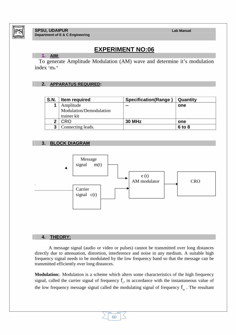
3. BLOCK DIAGRAM
fvbfggfsd ff
dfd
4. THEORY:
A message signal (audio or video or pulses) cannot be transmitted over long distances
directly due to attenuation, distortion, interference and noise in any medium. A suitable high frequency signal needs to be modulated by the low frequency band so that the message can be transmitted efficiently over long distances.
Modulation: . Modulation is a scheme which alters some characteristics of the high frequency signal, called the carrier signal of frequency f
c, in accordance with the instantaneous value of
the low frequency message signal called the modulating signal of frequency fm . The resultant
S.N. Item required Specification(Range ) Quantity 1 Amplitude
Modulation/Demodulation trainer kit
-- one
2 CRO 30 MHz one 3 Connecting leads. 6 to 8
e (t) AM modulator
Carrier signal c(t)
CRO
Message signal m(t)
SPSU, UDAIPUR Lab Manual Department of E & C Engineering
61
signal is called modulated signal. The resultant modulation is accordingly termed as Analog Modulation or Digital Modulation depending on whether the carrier is an Analog signal or a Digital signal. The Analog modulation can be either Amplitude modulation or Angle modulation (Phase modulation or Frequency modulation) for periodic continuous carrier waves (continuous in time domain) or Pulse modulation for pulsed carrier (not continuous in time domain). Amplitude Modulation (AM): It is a process in which the maximum amplitude of the carrier wave is varied linearly in accordance with instantaneous amplitude of modulating signal or base band signal. The waves can be voltage or current signals. The waveforms of the carrier wave, modulating wave and the resultant modulated wave are shown below. If the base band signal consists of single frequency it is called as single tone modulation. If the base band signal consists of more than one frequency it is called as multi tone modulation.
A carrier signal is represented by,
ec(t) = Ecmax sin (2ππππ fct+ΦΦΦΦc)
In amplitude modulation a voltage proportional to the modulating signal is added to the carrier amplitude. Then modulated carrier wave is given by,
e(t) = Ecmax +em(t) cos (2ππππfct+ΦΦΦΦc)
The term [Ecmax +em(t)] describes the envelop of the modulated wave. Modulation index: The ratio of maximum amplitude of the modulating signal to the maximum amplitude of carrier wave is defined as the amplitude modulation index and denoted by ‘ma ’. The modulation index is also known as depth of modulation or degree of modulation or modulation factor. Normally the value of ‘ma’ lies between 0 and 1. The modulation index is given by expression
ma = Vm / V
c
where, Vm = Amplitude of the modulating signal and
Vc = Amplitude of the carrier wave
It can be seen from the resultant of AM(single tone modulation) waveform
Vm = (V
max – V
min) / 2 …………………………….(1)
Vc = (V
max + V
min) / 2 ……………………………..(2)
SPSU, UDAIPUR Lab Manual Department of E & C Engineering
62
From (1) & (2)
ma =.(Vmax
– Vmin
) / (Vmax
+ Vmin
) ………………….(3)
Clearly, the Envelope of the modulated signals has the same shape as m(t) when m < 1. If the value of ‘ma’ exceeds 1, then the percentage modulation is greater than 100 and the base band signal is not preserved in the envelope. In this case the base band signal recovered from the envelope by the demodulator of a receiver will be distorted. This type of distortion is called envelope distortion and AM signal is called over modulated.
Expression for AM wave and frequency components : If single tone modulating signal
X(t) = Vm Cos wmt……….(4) and Carrier signal
C(t) = Vc Cos wct …….......(5) Then the modulated signal is given by S(t) = ( Vc + Vm Cos wmt )Cos wct……................(6)
On simplification, we get
S(t) = Vc { 1+ (Vm / Vc )Cos wmt }Cos wct = Vc { 1+ ma Cos wmt }Cos wct = Vc Cos wct + Vc ma Cos wmt Cos wct
= Vc Cos wct + [Vc ma Cos (wm + wc)t + Vc ma cos(wm-wc)t]/ 2
= Vc Cos2 Π fct + [Vc ma Cos 2Π (fc+ fm)t + Vc ma Cos 2Π (fc- fm)t]/ 2 ……… ……………………………(7)
Frequency spectrum: It is evident from the equation (7) that the frequency spectrum of the resultant modulated signal in case of single tone modulation consists of the original carrier
frequency fc as well as additional frequencies (f
c + f
m) called as upper side frequency and
(fc- f
m) called as lower side frequency. In case of multi tone modulation the base band
contains a range of frequencies from (fm + fm). In this case the frequency spectrum of the
resultant modulated signal consists of the original carrier frequency fc, an upper side band of
frequencies (fc + f
m) to (f
c + f
m + fm) and a lower side band of frequencies (f
c- f
m) to (f
c -
fm- fm).
SPSU, UDAIPUR Lab Manual Department of E & C Engineering
63
Methods of modulation & demodulation: Amplitude modulation is carried out by a circuit utilizing the nonlinear characteristic of solid state device like a diode called Square law modulator or collector circuit of a transistor called as collector modulator. It can be seen from the waveforms of the carrier wave, modulating wave and the resultant modulated wave that the envelope of the resultant waveform is identical to the modulating wave and thus utilized by the AM receiver for recovery of original message i.e. the modulating signal.
Benefits of modulation: (i) Efficient radiation (ii) Practicality of antenna (iii) Frequency translation
(iv) Multipl;exing (v) Remove interference (vi) Reduction of noise
5. EXPERIMENTAL PROCEDURE : 1. Make the connection according to the block diagram 2. Switch on the power supply .Connect 1 KHz, 2V AF Generator to CRO and note the frequency and amplitude of AF output. . 3. Similarly note the output amplitude and frequency of RF Carrier wave. 4. Set the amplitude of AF generator and amplitude of carrier wave so that modulated output can be observed conveniently by easy manipulation of CRO. 5. Note down the values of V
max and V
min.
6. Change the amplitude of AF Generator to different values, keeping RF output constant and note down the corresponding values of V
max and V
min.
7. Calculate amplitude modulation index ma =.(Vmax
– Vmin
) / (Vmax
+ Vmin
) 8. Repeat step No.6 and tabulate the results. 9. Draw wave forms as observed on CRO and label the different waveforms appropriately
SPSU, UDAIPUR Lab Manual Department of E & C Engineering
64
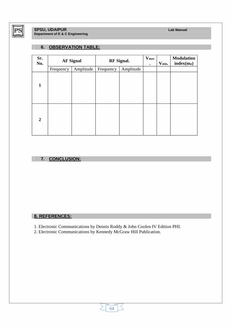
6. OBSERVATION TABLE:
Sr. No. AF Signal RF Signal. Vmax
.
Vmin. Modulation index(ma)
Frequency Amplitude Frequency Amplitude
1
2
7. CONCLUSION: 8. REFERENCES: 1. Electronic Communications by Dennis Roddy & John Coolen IV Edition PHI. 2. Electronic Communications by Kennedy McGraw Hill Publication.
SPSU, UDAIPUR Lab Manual Department of E & C Engineering
65
9 QUESTIONS:
Q. 1. What is modulation? Q. 2. Which are the three discrete frequencies in AM? Q. 3 How many sidebands in AM? Q. 4. What is the unit of modulation index in AM? Q. 5. Where the modulation index lies?
SPSU, UDAIPUR Lab Manual Department of E & C Engineering
66
EXPERIMENT NO:07 1. AIM:
To demodulate amplitude modulated wave
2. APPARATUS REQUIRED:
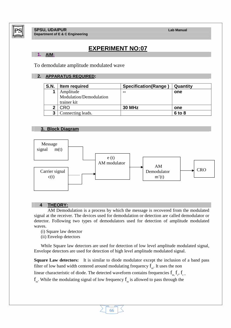
3. Block Diagram
fvbfggfsd ff
dfd
4 THEORY:
AM Demodulation is a process by which the message is recovered from the modulated signal at the receiver. The devices used for demodulation or detection are called demodulator or detector. Following two types of demodulators used for detection of amplitude modulated waves.
(i) Square law detector (ii) Envelop detectors
While Square law detectors are used for detection of low level amplitude modulated signal, Envelope detectors are used for detection of high level amplitude modulated signal.
Square Law detectors: It is similar to diode modulator except the inclusion of a band pass filter of low band width centered around modulating frequency f
m. It uses the non
linear characteristic of diode. The detected waveform contains frequencies fm,
fc, f
c +
fm. While the modulating signal of low frequency f
m is allowed to pass through the
S.N. Item required Specification(Range ) Quantity 1 Amplitude
Modulation/Demodulation trainer kit
-- one
2 CRO 30 MHz one 3 Connecting leads. 6 to 8
e (t) AM modulator
Carrier signal c(t)
AM Demodulator m’(t)
Message signal m(t)
CRO
SPSU, UDAIPUR Lab Manual Department of E & C Engineering
67
filter, the high frequency carrier signal fc as well as upper side band f
c +f
m and lower
side band of frequency fc-
fm are rejected.
Envelope detectors: Modulated signal output of receiver IF amplifier tuned circuit is passed through the Envelope diode detector which has a parallel combination of R & C as the load resistance across which rectified output voltage is developed .At its positive peak of the RF cycle, C charges up to a potential almost to a peak signal voltage. The difference is due to the diode drop since the forward resistance is small. Between peaks a little of the charge in C decays through R, to be replenished at the next positive peak. The result is output envelope which resembles the original modulating message signal. AGC circuit is used at the output of the De-Modulator. In this demodulator the time constant RC is a critical parameter. If the value of RC is very high, the capacitor C discharges slowly and in the process, the envelope does not follow the modulating signal , if the amplitude of the later is decreasing and of negative slope. This results in clipping of the amplitude of envelope. On the other hand if the value of RC is very low, the capacitor C discharges very fast to a value lesser than the peak amplitude of next positive cycle even before the arrival of peak value of next positive cycle. This results in saw tooth type envelope. The resultant demodulated wave form is a highly distorted form of original modulating signal under both condition of very high RC or very low RC. The distortion is least only when the value of RC is chosen properly. WAVEFORMS:
An example of Amplitude Demodulation. The top diagram shows the detected modulating signal of low frequency as well as the high frequency carrier wave. The bottom diagram shows the amplitude modulated signal. Notice how the peaks of the modulated output follow the cantour of the original modulating signal.
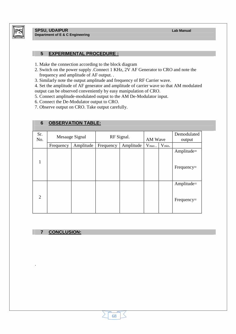
SPSU, UDAIPUR Lab Manual Department of E & C Engineering
68
5 EXPERIMENTAL PROCEDURE :
1. Make the connection according to the block diagram 2. Switch on the power supply .Connect 1 KHz, 2V AF Generator to CRO and note the frequency and amplitude of AF output. . 3. Similarly note the output amplitude and frequency of RF Carrier wave. 4. Set the amplitude of AF generator and amplitude of carrier wave so that AM modulated output can be observed conveniently by easy manipulation of CRO. 5. Connect amplitude-modulated output to the AM De-Modulator input. 6. Connect the De-Modulator output to CRO. 7. Observe output on CRO. Take output carefully.
6 OBSERVATION TABLE:
Sr. No.
Mesaage Signal RF Signal.
AM Wave Demodulated
output Frequency Amplitude Frequency Amplitude Vmax . Vmin.
1
Amplitude= Frequency=
2
Amplitude= Frequency=
7 CONCLUSION:
.
SPSU, UDAIPUR Lab Manual Department of E & C Engineering
69
8. REFERENCES: 1. Electronic Communications by Dennis Roddy & John Coolen IV Edition PHI. 2. Electronic Communications by Kennedy McGraw Hill Publication.
8. QUESTIONS: Q.1. What is the most commonly used demodulator? Q.2. What is the required oscillator frequency in AM receiver? Q.3. How AM signals with large carrier are detected? Q.4. How much bandwidth required for AM wave? Q.5. List out the advantages of Amplitude modulation.
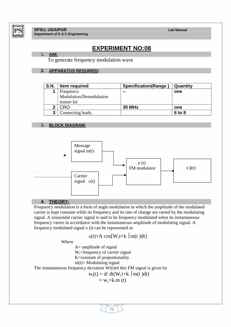
SPSU, UDAIPUR Lab Manual Department of E & C Engineering
70
EXPERIMENT NO:08 1. AIM:
To generate frequency modulation wave
2. APPARATUS REQUIRED:
3. BLOCK DIAGRAM:
fvbfggfsd ff
dfd
4. THEORY: Frequency modulation is a form of angle modulation in which the amplitude of the modulated carrier is kept constant while its frequency and its rate of change are varied by the modulating signal. A sinusoidal carrier signal is said to be frequency modulated when its instantaneous frequency varies in accordance with the instantaneous amplitude of modulating signal. A frequency modulated signal x (t) can be represented as
x(t)+A cos[Wct+k ∫ m(t )dt] Where
A= amplitude of signal Wc=frequency of carrier signal K=constant of proportionality m(t)= Modulating signal
The instantaneous frequency deviation Wi(t)of this FM signal is given by wi(t) = d/ dt(Wct+k ∫ m(t )dt)
= wc+k.m (t)
S.N. Item required Specification(Range ) Quantity 1 Frequency
Modulation/Demodulation trainer kit
-- one
2 CRO 30 MHz one 3 Connecting leads. 6 to 8
e (t) FM modulator
Carrier signal c(t)
CRO
Message signal m(t)
SPSU, UDAIPUR Lab Manual Department of E & C Engineering
71
The instantaneous frequency deviation wi(t)= wi(t)-wc and therefore wi(t)=K.m(t)
The ratio of the maximum frequency deviation i.e. w to the modulating signal frequency Wm is known as modulation index,mf
mf = w/wm
According to band width of fm signal, B is given by
B=2(mf+1) fm
With mf rounded off to next higher integer.
An important concept in the understanding of FM is that of frequency deviation. The amount of frequency deviation a signal experiences is a measure of the change in transmitter output frequency from the rest frequency of the transmitter. The rest frequency of a transmitter is defined as the output frequency wit no modulating signal applied. For a transmitter with linear modulation characteristics, the frequency deviation of the carrier is directly proportional to the amplitude of the applied modulating signal. The index of modulation, mf, is given by the following relationship
mf=δ/fM
As can be seen from the equation, mf is equal to the peak deviation caused when the signal is modulated by the frequency of the modulating signal; therefore, mf is a function of both the modulating signal amplitude and frequency. Furthermore, mf can take on any value from 0 to infinity. Its range is not limited as it is for AM. The practical implementation of FM communication systems in a limited bandwidth-channel environment, such as cellular radio, requires a limitation upon the maximum frequency deviation to prevent adjacent channel interference. For example, the FCC’s Rules and Regulations limit FM broadcast-band transmitters to a maximum frequency deviation of 75 kHz. The maximum allowable deviation will be assigned the value of 100% modulation. Therefore, in equation form, the percentage of modulation is given by:
% Modulation= δ*100/δmax Frequency Deviation: It is the amount by which carrier frequency is varied from its unmodulated value and it is same as frequency variation.
Max Frequency deviation W =KX(t)。max
Very often we write W = h ; Maxium allowed deviation =75 khz Frequency Modulation Index (mf )- It is the ratio of frequency deviation W in rad/sec to the
angular frequency of modulating signal Wm or frequency deviation in Hertz/sec to to the
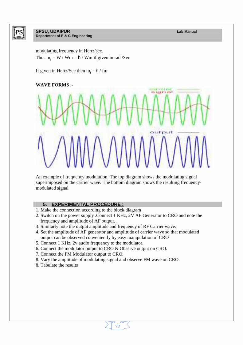
SPSU, UDAIPUR Lab Manual Department of E & C Engineering
72
modulating frequency in Hertz/sec.
Thus mf = W / Wm = h / Wm if given in rad /Sec
If given in Hertz/Sec then mf = h / fm
WAVE FORMS :-
An example of frequency modulation. The top diagram shows the modulating signal superimposed on the carrier wave. The bottom diagram shows the resulting frequency-modulated signal
5. EXPERIMENTAL PROCEDURE :
1. Make the connection according to the block diagram 2. Switch on the power supply .Connect 1 KHz, 2V AF Generator to CRO and note the frequency and amplitude of AF output. . 3. Similarly note the output amplitude and frequency of RF Carrier wave. 4. Set the amplitude of AF generator and amplitude of carrier wave so that modulated output can be observed conveniently by easy manipulation of CRO 5. Connect 1 KHz, 2v audio frequency to the modulator. 6. Connect the modulator output to CRO & Observe output on CRO. 7. Connect the FM Modulator output to CRO. 8. Vary the amplitude of modulating signal and observe FM wave on CRO. 8. Tabulate the results
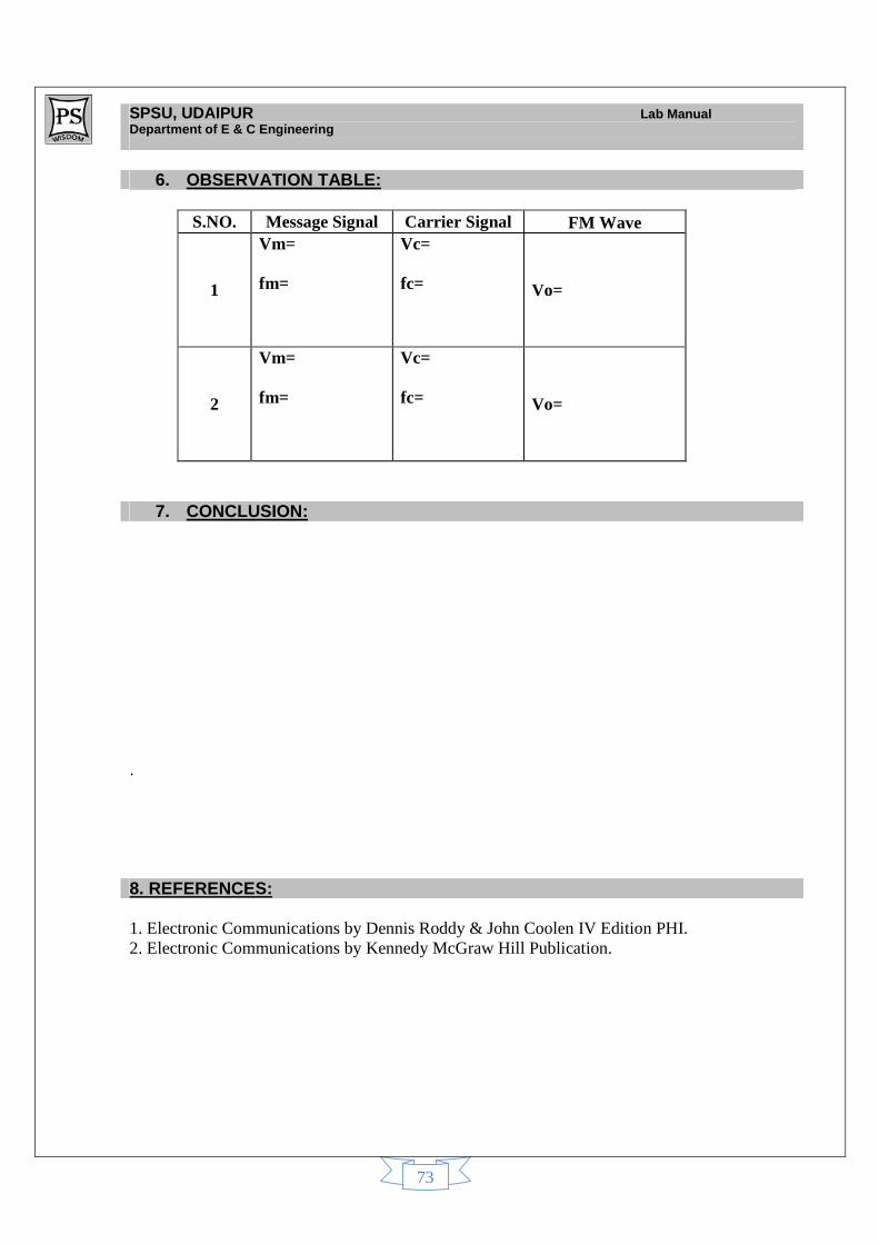
SPSU, UDAIPUR Lab Manual Department of E & C Engineering
73
6. OBSERVATION TABLE:
S.NO. Message Signal Carrier Signal FM Wave
1
Vm= fm=
Vc= fc= Vo=
2
Vm= fm=
Vc= fc= Vo=
7. CONCLUSION: . 8. REFERENCES: 1. Electronic Communications by Dennis Roddy & John Coolen IV Edition PHI. 2. Electronic Communications by Kennedy McGraw Hill Publication.
SPSU, UDAIPUR Lab Manual Department of E & C Engineering
74
9. QUESTIONS:
Q.1. What frequency deviation in FM? Q.2. Which is the useful parameter for determination of bandwidth? Q.3. How many sidebands in FM? Q.4. Which are significant sidebands? . Q.5. What is VCO?
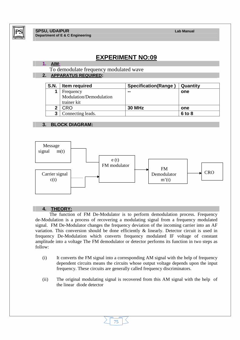
SPSU, UDAIPUR Lab Manual Department of E & C Engineering
75
EXPERIMENT NO:09
1. AIM: To demodulate frequency modulated wave
2. APPARATUS REQUIRED:
3. BLOCK DIAGRAM:
fvbfggfsd ff
dfd
4. THEORY:
The function of FM De-Modulator is to perform demodulation process. Frequency de-Modulation is a process of recovering a modulating signal from a frequency modulated signal. FM De-Modulator changes the frequency deviation of the incoming carrier into an AF variation. This conversion should be done efficiently & linearly. Detector circuit is used in frequency De-Modulation which converts frequency modulated IF voltage of constant amplitude into a voltage The FM demodulator or detector performs its function in two steps as follow:
(i) It converts the FM signal into a corresponding AM signal with the help of frequency dependent circuits means the circuits whose output voltage depends upon the input frequency. These circuits are generally called frequency discriminators.
(ii) The original modulating signal is recovered from this AM signal with the help of the linear diode detector
S.N. Item required Specification(Range ) Quantity 1 Frequency
Modulation/Demodulation trainer kit
-- one
2 CRO 30 MHz one 3 Connecting leads. 6 to 8
e (t) FM modulator
Carrier signal c(t)
FM Demodulator m’(t)
Message signal m(t)
CRO
SPSU, UDAIPUR Lab Manual Department of E & C Engineering
76
Types of FM Demodulator 1. Slope Detector
The principle of operation of Slope detector depends upon the slope of the frequency response characteristics of a frequency selective network .The two main FM detectors , which use detuned resonant circuits come under this category, are:
(i) Single-tuned detector circuit or simple slope detector. (ii) Staggered tuned detector circuit or balanced slope detector 2. Phase Difference Detectors The following two circuits come under this category: (i) Foster-Seely Detector (ii) Ratio detector
The circuit consists of a tuned circuit which is slightly detuned from the carrier frequency fc. In other words, the circuits uses two tuned circuits which are tuned to two different frequencies. First one is tuned to the incoming FM carrier frequency fc whereas the second one is tuned to a frequency slightly different from the carrier frequency fc. Therefore, this portion of the circuit which contains two tuned circuits tuned to different frequencies, is called discriminator. This circuit converts the FM signal into an AM signal as shown in the slope detector characteristics curve. The another portion of the circuit is envelope detector. The AM signal from the output of the discriminator is applied at the input of envelope detector. At the output of envelope detector, the original modulating or base band signal is obtained.
Although this circuit is simple and inexpensive, it has following drawbacks.
(i) The circuits non-linear characteristics produces a harmonic distortion .The non-linearity is obvious from the fact that the slope is not the same at each point of the characteristics.
(ii) The circuit does not eliminate the amplitude variations and the output is sensitive to any amplitude variations in the input FM signal which is obviously not a desirable feature. A good discriminator circuit must respond variations and not to amplitude variations.
Foster-seely detectors: Widely used FM De-Modulator is Foster-Seely discriminator especially in FM radio receivers, wide band or narrow band. The ratio detector is a good FM De-Modulator, also widely used in practice, especially in TV receivers.
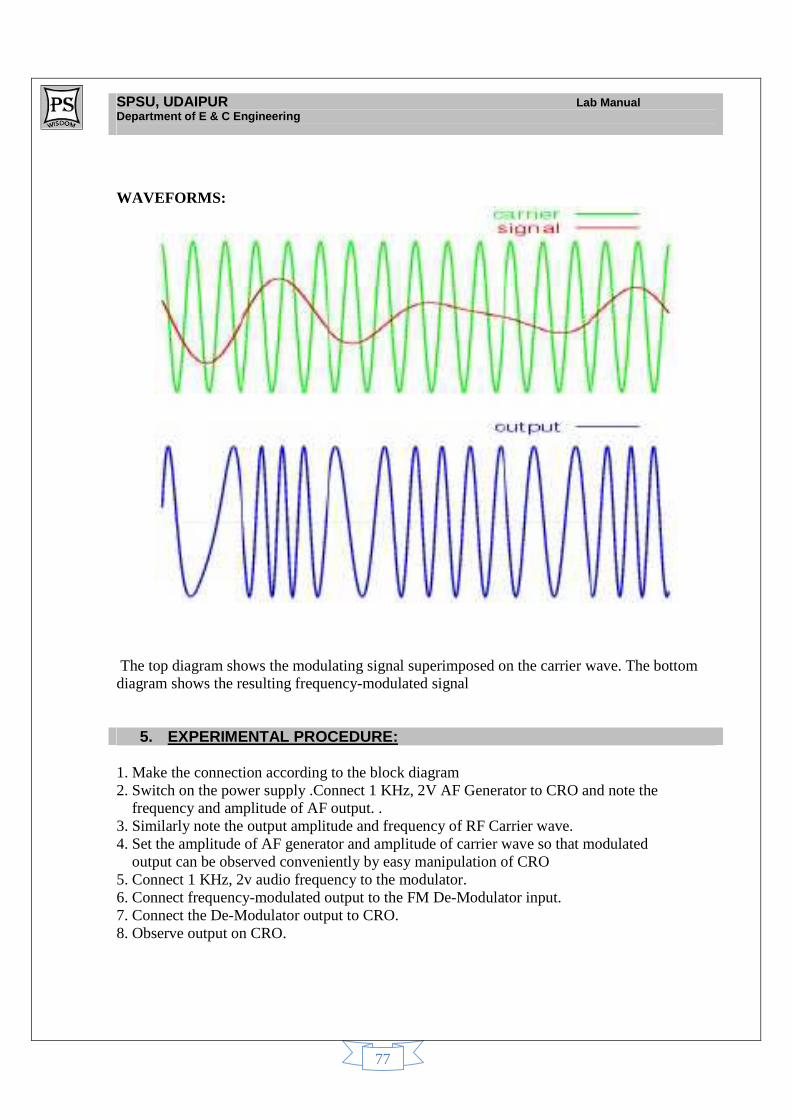
SPSU, UDAIPUR Lab Manual Department of E & C Engineering
77
WAVEFORMS:
The top diagram shows the modulating signal superimposed on the carrier wave. The bottom diagram shows the resulting frequency-modulated signal
5. EXPERIMENTAL PROCEDURE:
1. Make the connection according to the block diagram 2. Switch on the power supply .Connect 1 KHz, 2V AF Generator to CRO and note the frequency and amplitude of AF output. . 3. Similarly note the output amplitude and frequency of RF Carrier wave. 4. Set the amplitude of AF generator and amplitude of carrier wave so that modulated output can be observed conveniently by easy manipulation of CRO 5. Connect 1 KHz, 2v audio frequency to the modulator. 6. Connect frequency-modulated output to the FM De-Modulator input. 7. Connect the De-Modulator output to CRO. 8. Observe output on CRO.
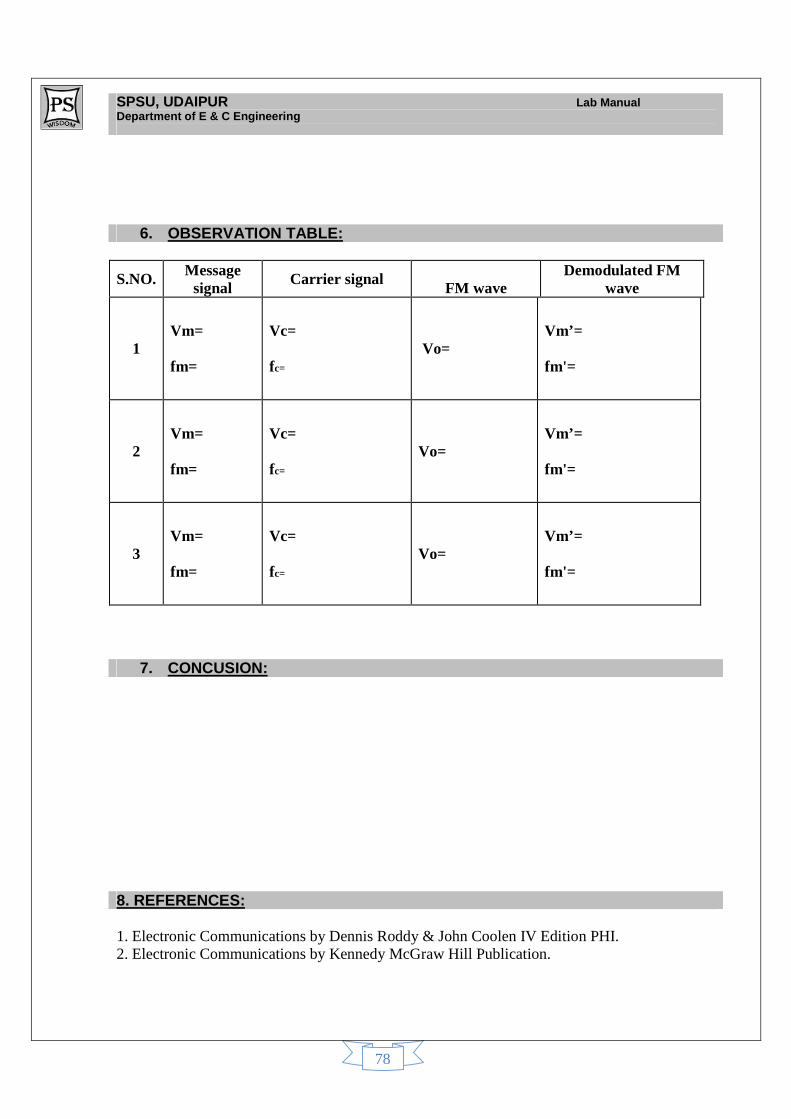
SPSU, UDAIPUR Lab Manual Department of E & C Engineering
78
6. OBSERVATION TABLE:
S.NO. Message signal
Carrier signal FM wave
Demodulated FM wave
1 Vm= fm=
Vc= fc=
Vo= Vm’= fm'=
2 Vm= fm=
Vc= fc=
Vo= Vm’= fm'=
3 Vm= fm=
Vc= fc=
Vo= Vm’= fm'=
7. CONCUSION:
8. REFERENCES: 1. Electronic Communications by Dennis Roddy & John Coolen IV Edition PHI. 2. Electronic Communications by Kennedy McGraw Hill Publication.
SPSU, UDAIPUR Lab Manual Department of E & C Engineering
79
9.QUESTIONS:
Q.1. what is modulation index in FM? Q.2. Why the power is same in FM modulation and demodulation? Q.3. Write the two types of phase difference discriminator? Q.4. write the disadvantage of balanced slope discriminator? Q.5. what is the merit of ratio detector?
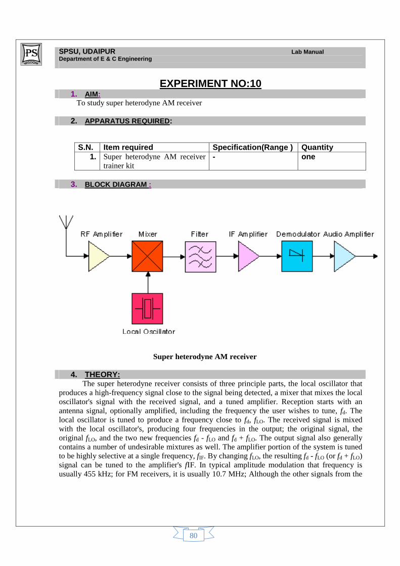
SPSU, UDAIPUR Lab Manual Department of E & C Engineering
80
EXPERIMENT NO:10 1. AIM:
To study super heterodyne AM receiver
2. APPARATUS REQUIRED:
3. BLOCK DIAGRAM :
Super heterodyne AM receiver
4. THEORY:
The super heterodyne receiver consists of three principle parts, the local oscillator that produces a high-frequency signal close to the signal being detected, a mixer that mixes the local oscillator's signal with the received signal, and a tuned amplifier. Reception starts with an antenna signal, optionally amplified, including the frequency the user wishes to tune, fd. The local oscillator is tuned to produce a frequency close to fd, fLO. The received signal is mixed with the local oscillator's, producing four frequencies in the output; the original signal, the original fLO, and the two new frequencies fd - fLO and fd + fLO. The output signal also generally contains a number of undesirable mixtures as well. The amplifier portion of the system is tuned to be highly selective at a single frequency, fIF. By changing fLO, the resulting fd - fLO (or fd + fLO) signal can be tuned to the amplifier's fIF. In typical amplitude modulation that frequency is usually 455 kHz; for FM receivers, it is usually 10.7 MHz; Although the other signals from the
S.N. Item required Specification(Range ) Quantity 1. Super heterodyne AM receiver
trainer kit - one
SPSU, UDAIPUR Lab Manual Department of E & C Engineering
81
mixed output of the heterodyne are still present when they reach the amplifier, they are either filtered out or simply left un-amplified.
The diagram above shows the basic elements of a single conversion super heterodyne receiver. In practice not every design will have all these elements, nor does this convey the complexity of other designs, but the essential elements of a local oscillator and a mixer followed by a filter and IF amplifier are common to all heterodyne circuits. Cost-optimized designs may use one active device for both local oscillator and mixer—this is sometimes called a "converter" stage. The advantage to this method is that most of the radio's signal path has to be sensitive to only a narrow range of frequencies. Only the front end (the part before the frequency converter stage) needs to be sensitive to a wide frequency range. For example, the front end might need to be sensitive to 1–30 MHz, while the rest of the radio might need to be sensitive only to 455 kHz, a typical IF. Only one or two tuned stages need to be adjusted to track over the tuning range of the receiver; all the intermediate-frequency stages operate at a fixed frequency which need not be adjusted. Sometimes, to overcome obstacles such as image response, more than one IF is used. In such a case, the front end might be sensitive to 1–30 MHz, the first half of the radio to 5 MHz, and the last half to 50 kHz.
The IF Amplifier in this receiver consists of two stages of amplification and provides the main signal amplification and selectivity. Operating at a fixed IF frequency means that the design of the amplifier can be simplified. If it were not the fixed frequency, all the amplifier may need to be tunable across the whole range of incoming RF frequencies and it would be difficult to arrange for the amplifier to keep in step as they are re-tuned. In addition, the radio must select the wanted transmission and reject all the others. To do this the band pass of all stages must carefully controlled. Each IF stage does not necessary has the same band pass characteristics. The overall response is important. Again, this is something which is much more easily achieved without the added complication of making them tunable. At the final output from the IF amplifiers, we have a 455 KHz wave which is amplitude modulated by the wanted audio information. The selectivity of the IF amplifiers has removed the unwanted components generated by the mixing process. Occasionally special-purpose receivers will use an intermediate frequency much higher than the signal, in order to obtain very high image rejection. Super heterodyne receivers have superior characteristics to simpler receiver types in frequency stability and selectivity. They offer much better stability than Tuned radio frequency receivers (TRF) because a tunable oscillator is more easily stabilized than a tunable filter, especially with modern frequency synthesizer technology. IF filters can give much narrower pass bands at the same Q factor than an equivalent RF filter. A fixed IF also allows the use of a crystal filter in very critical designs such as radiotelephone receivers, in which exceptionally high selectivity is necessary.
The amount that a signal is down-shifted by the local oscillator depends on whether its frequency f is higher or lower than fLO. That is because its new frequency is |f − fLO| in either case. Therefore, there are potentially two signals that could both shift to the same fIF one at f = fLO + fIF and another at f = fLO − fIF. One or the other of those signals has to be filtered out prior to the mixer to avoid aliasing. When the upper one is filtered out, it is called high-side injection, because fLO is above the frequency of the received signal. The other case is called low-side injection.
One major disadvantage to the super heterodyne receiver is the problem of image frequency. In heterodyne receivers, an image frequency is an undesired input frequency equal to the station frequency plus twice the intermediate frequency. The image frequency results in two
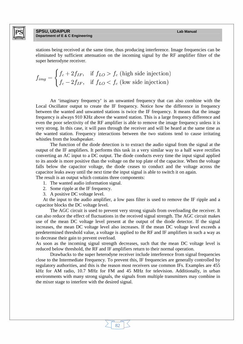
SPSU, UDAIPUR Lab Manual Department of E & C Engineering
82
stations being received at the same time, thus producing interference. Image frequencies can be eliminated by sufficient attenuation on the incoming signal by the RF amplifier filter of the super heterodyne receiver.
An ‘imaginary frequency’ is an unwanted frequency that can also combine with the Local Oscillator output to create the IF frequency. Notice how the difference in frequency between the wanted and unwanted stations is twice the IF frequency. It means that the image frequency is always 910 KHz above the wanted station. This is a large frequency difference and even the poor selectivity of the RF amplifier is able to remove the image frequency unless it is very strong. In this case, it will pass through the receiver and will be heard at the same time as the wanted station. Frequency interactions between the two stations tend to cause irritating whistles from the loudspeaker.
The function of the diode detection is to extract the audio signal from the signal at the output of the IF amplifiers. It performs this task in a very similar way to a half wave rectifies converting an AC input to a DC output. The diode conducts every time the input signal applied to its anode is more positive than the voltage on the top plate of the capacitor. When the voltage falls below the capacitor voltage, the diode ceases to conduct and the voltage across the capacitor leaks away until the next time the input signal is able to switch it on again. The result is an output which contains three components:
1. The wanted audio information signal. 2. Some ripple at the IF frequency. 3. A positive DC voltage level. At the input to the audio amplifier, a low pass filter is used to remove the IF ripple and a
capacitor blocks the DC voltage level. The AGC circuit is used to prevent very strong signals from overloading the receiver. It
can also reduce the effect of fluctuations in the received signal strength. The AGC circuit makes use of the mean DC voltage level present at the output of the diode detector. If the signal increases, the mean DC voltage level also increases. If the mean DC voltage level exceeds a predetermined threshold value, a voltage is applied to the RF and IF amplifiers in such a way as to decrease their gain to prevent overload. As soon as the incoming signal strength decreases, such that the mean DC voltage level is reduced below threshold, the RF and IF amplifiers return to their normal operation.
Drawbacks to the super heterodyne receiver include interference from signal frequencies close to the Intermediate Frequency. To prevent this, IF frequencies are generally controlled by regulatory authorities, and this is the reason most receivers use common IFs. Examples are 455 kHz for AM radio, 10.7 MHz for FM and 45 MHz for television. Additionally, in urban environments with many strong signals, the signals from multiple transmitters may combine in the mixer stage to interfere with the desired signal.
SPSU, UDAIPUR Lab Manual Department of E & C Engineering
83
5. CONCUSION:
6. REFERENCES: 1. Electronic Communications by Dennis Roddy & John Coolen IV Edition PHI. 2. Electronic Communications by Kennedy McGraw Hill Publication.
7 QUESTIONS: 1. Define ‘selectivity’ with respect to super heterodyne receiver.
2. What is role of delayed AGC in AM receiver?
3. A receiver has poor IF selectivity. Therefore, it will have also poor___________.
4. Define the term ‘fidelity’ with respect to super heterodyne receiver. 5. AM broadcast frequency ranges from _________ to ______________.