Clustering and The Expectation-MaximizationAlgorithm

Unsupervised Learning

Marek Petrik

3/7

Some of the figures in this presentation are taken from ”An Introduction to Statistical Learning, with applications in R”(Springer, 2013) with permission from the authors: G. James, D. Wi�en, T. Hastie and R. Tibshirani

Learning Methods

1. Supervised Learning: Learning a function f :

Y = f(X) + ε

1.1 Regression1.2 Classification

2. Unsupervised learning: Discover interesting properties ofdata (no labels)

X1, X2, . . .

2.1 Dimensionality reduction or embedding2.2 Clustering

Principal Components Analysis

I Reduce dimensionalityI Start with features X1 . . . Xn

I Construct fewer features Z1 . . . ZM

Z1 = φ11X1 + φ21X2 + . . .+ φp1Xp

I Weights are usually normalized (using `2 norm)

p∑j=1

φ2j1 = 1

I Data has greatest variance along Z1

1st Principal Component

10 20 30 40 50 60 70

05

10

15

20

25

30

35

Population

Ad S

pendin

g

I 1st Principal Component: Direction with the largest variance

Z1 = 0.839× (pop− pop) + 0.544× (ad− ad)

More Unsupervised Learning: Discovering Structure ofData

1. K-Means Clustering

2. Hierarchical Clustering

3. Expectation-Maximization Method (Not Covered in ISL, seeESL 8.5)

Clustering

Simplify data in a di�erent way than PCA.

I PCA finds a low-dimensional representation of data

I Clustering finds homogeneous subgroups among theobservations

Clustering: Assumptions and Goals

I Exists a method for measuring similarity between data pointsI Some points are more similar than others

I Want to identify similarity pa�erns1. Discover the di�erent types of disease2. Market segmentation: Types of users that visit a website3. Discover movie or book genres4. Discover types of topics in documents

I Discover latent pa�erns that exist but may not beobserved/observable

Clustering: Assumptions and Goals

I Exists a method for measuring similarity between data pointsI Some points are more similar than others

I Want to identify similarity pa�erns1. Discover the di�erent types of disease2. Market segmentation: Types of users that visit a website3. Discover movie or book genres4. Discover types of topics in documents

I Discover latent pa�erns that exist but may not beobserved/observable

Clustering Algorithms

I K-Means: simple and e�ectiveI Hierarchical clustering: Many complex clustersI Many other clustering methods, most heuristicsI EM: General algorithm for dealing with latent variables by

maximizing likelihood

K-Means Clustering

I Cluster data into complete and non-overlapping setsI Example:

K=2 K=3 K=4

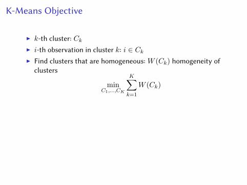
K-Means Objective

I k-th cluster: CkI i-th observation in cluster k: i ∈ Ck

I Find clusters that are homogeneous: W (Ck) homogeneity ofclusters

minC1,...,CK

K∑k=1

W (Ck)

I Define homogeneity as in-cluster variance

minC1,...,CK

K∑k=1

1

|Ck|∑

i,i′∈Ck

p∑j=1

(xij − xi′j)2

I This is an NP hard problem

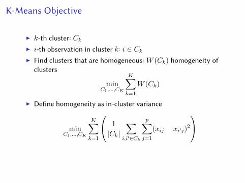
K-Means Objective

I k-th cluster: CkI i-th observation in cluster k: i ∈ CkI Find clusters that are homogeneous: W (Ck) homogeneity of

clusters

minC1,...,CK

K∑k=1

W (Ck)

I Define homogeneity as in-cluster variance

minC1,...,CK

K∑k=1

1

|Ck|∑

i,i′∈Ck

p∑j=1

(xij − xi′j)2

I This is an NP hard problem

K-Means Objective

I k-th cluster: CkI i-th observation in cluster k: i ∈ CkI Find clusters that are homogeneous: W (Ck) homogeneity of

clusters

minC1,...,CK

K∑k=1

W (Ck)

I Define homogeneity as in-cluster variance

minC1,...,CK

K∑k=1

1

|Ck|∑

i,i′∈Ck

p∑j=1

(xij − xi′j)2

I This is an NP hard problem

K-Means Objective

I k-th cluster: CkI i-th observation in cluster k: i ∈ CkI Find clusters that are homogeneous: W (Ck) homogeneity of

clusters

minC1,...,CK

K∑k=1

W (Ck)

I Define homogeneity as in-cluster variance

minC1,...,CK

K∑k=1

1

|Ck|∑

i,i′∈Ck

p∑j=1

(xij − xi′j)2

I This is an NP hard problem

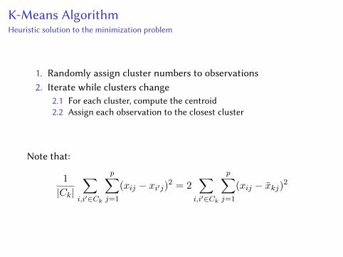
K-Means AlgorithmHeuristic solution to the minimization problem

1. Randomly assign cluster numbers to observations2. Iterate while clusters change

2.1 For each cluster, compute the centroid2.2 Assign each observation to the closest cluster

Note that:

1

|Ck|∑

i,i′∈Ck

p∑j=1

(xij − xi′j)2 = 2∑

i,i′∈Ck

p∑j=1

(xij − x̄kj)2

K-Means Illustration

Data Step 1 Iteration 1, Step 2a

Iteration 1, Step 2b Iteration 2, Step 2a Final Results

Properties of K-Means

I Local minimum: Does not necessarily find the optimal solutionI Multiple runs can result in di�erent solutionsI Choose the result of the run with minimal objectiveI Cluster labels do not ma�er

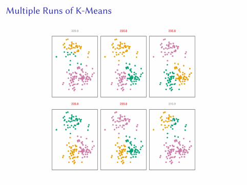
Multiple Runs of K-Means

320.9 235.8 235.8

235.8 235.8 310.9

Hierarchical Clustering

I Multiple levels of similarity needed in complex domainsI Build a similarity tree

3

4

1 6

9

2

8

5 7

0.0

0.5

1.0

1.5

2.0

2.5

3.0

1

2

3

4

5

6

7

8

9

−1.5 −1.0 −0.5 0.0 0.5 1.0

−1

.5−

1.0

−0

.50

.00

.5

X1

X2

Dendrogram: Similarity Tree0

24

68

10

02

46

81

0

02

46

81

0

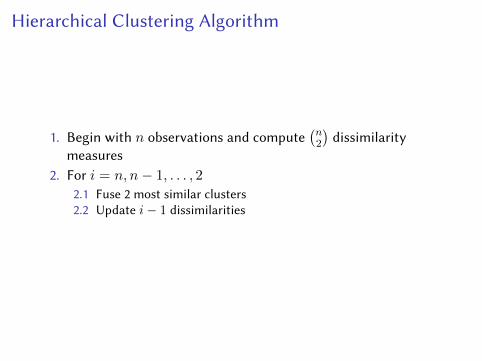
Hierarchical Clustering Algorithm

1. Begin with n observations and compute(n2

)dissimilarity

measures2. For i = n, n− 1, . . . , 2

2.1 Fuse 2 most similar clusters2.2 Update i− 1 dissimilarities

Hierarchical Clustering Algorithm: Illustration

1

2

3

4

5

6

7

8

9

−1.5 −1.0 −0.5 0.0 0.5 1.0

−1.5

−1.0

−0.5

0.0

0.5

1

2

3

4

5

6

7

8

9

−1.5 −1.0 −0.5 0.0 0.5 1.0

−1.5

−1.0

−0.5

0.0

0.5

1

2

3

4

5

6

7

8

9

−1.5 −1.0 −0.5 0.0 0.5 1.0

−1.5

−1.0

−0.5

0.0

0.5

1

2

3

4

5

6

7

8

9

−1.5 −1.0 −0.5 0.0 0.5 1.0

−1.5

−1.0

−0.5

0.0

0.5

X1X1

X1X1

X2

X2

X2

X2

Dissimilarity Measure: Linkage

1. Complete

2. Single

3. Average

4. Centroid

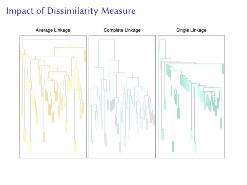
Impact of Dissimilarity Measure

Average Linkage Complete Linkage Single Linkage

Clustering in Practice

I Fraught with problems: no clear measure of quality (like MSE)I How to choose k? Problem dependentI Standardize features, center them?I What dissimilarity to use?

I Careful over-explaining clustering results: source:http://miriamposner.com

Clustering in Practice

I Fraught with problems: no clear measure of quality (like MSE)I How to choose k? Problem dependentI Standardize features, center them?I What dissimilarity to use?I Careful over-explaining clustering results: source:

http://miriamposner.com

Expectation-Maximization

I Maximum likelihood approach to clusteringI General method for dealing with latent features / labelsI Especially useful with generative modelsI A heuristic method used to solve complex optimization

problemsI Generalization of the idea: Minorization-MaximizationI Gentle introduction: https://www.cs.utah.edu/∼piyush/teaching/EM algorithm.pdf

Recall LDA

LDA: Linear Discriminant Analysis

I Generative model: capture probability of predictors for eachlabel

−4 −2 0 2 4 −3 −2 −1 0 1 2 3 4

01

23

45

I Predict:

1. Pr[balance | default = yes] and Pr[default = yes]2. Pr[balance | default = no] and Pr[default = no]

I Classes are normal: Pr[balance | default = yes]

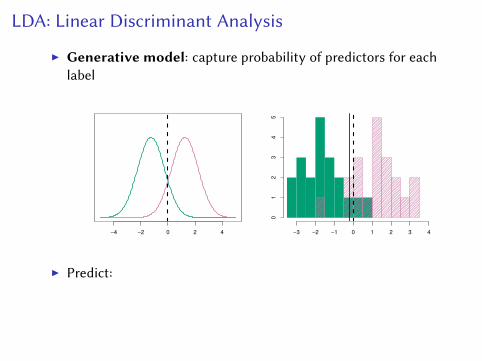
LDA: Linear Discriminant Analysis

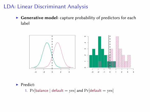
I Generative model: capture probability of predictors for eachlabel

−4 −2 0 2 4 −3 −2 −1 0 1 2 3 4

01

23

45

I Predict:1. Pr[balance | default = yes] and Pr[default = yes]

2. Pr[balance | default = no] and Pr[default = no]

I Classes are normal: Pr[balance | default = yes]

LDA: Linear Discriminant Analysis

I Generative model: capture probability of predictors for eachlabel

−4 −2 0 2 4 −3 −2 −1 0 1 2 3 4

01

23

45

I Predict:1. Pr[balance | default = yes] and Pr[default = yes]2. Pr[balance | default = no] and Pr[default = no]

I Classes are normal: Pr[balance | default = yes]

LDA: Linear Discriminant Analysis

I Generative model: capture probability of predictors for eachlabel

−4 −2 0 2 4 −3 −2 −1 0 1 2 3 4

01

23

45

I Predict:1. Pr[balance | default = yes] and Pr[default = yes]2. Pr[balance | default = no] and Pr[default = no]

I Classes are normal: Pr[balance | default = yes]

LDA vs Logistic Regression

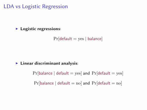
I Logistic regressions:

Pr[default = yes | balance]

I Linear discriminant analysis:

Pr[balance | default = yes] and Pr[default = yes]

Pr[balance | default = no] and Pr[default = no]

LDA with 1 Feature

I Classes are normal and class probabilities πk are scalars

fk(x) =1

σ√

2πexp

(− 1

2σ2(x− µk)2

)I Key Assumption:Class variances σ2k are the same.

−4 −2 0 2 4 −3 −2 −1 0 1 2 3 4

01

23

45

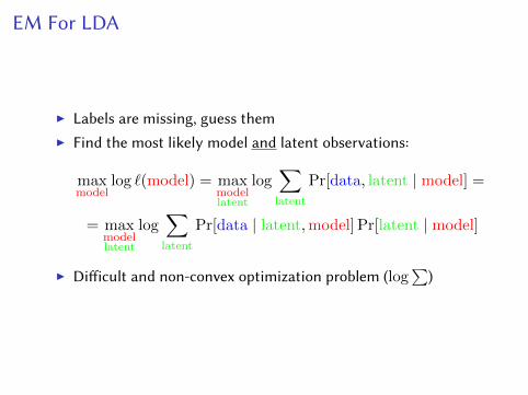
EM For LDA

I Labels are missing, guess themI Find the most likely model and latent observations:

maxmodel

log `(model) = maxmodellatent

log∑latent

Pr[data, latent | model] =

= maxmodellatent

log∑latent

Pr[data | latent,model] Pr[latent | model]

I Di�icult and non-convex optimization problem (log∑

)

EM For LDA

I Labels are missing, guess themI Find the most likely model and latent observations:

maxmodel

log `(model) = maxmodellatent

log∑latent

Pr[data, latent | model] =

= maxmodellatent

log∑latent

Pr[data | latent,model] Pr[latent | model]

I Di�icult and non-convex optimization problem (log∑

)

EM For LDA

I Labels are missing, guess themI Find the most likely model and latent observations:

maxmodel

log `(model) = maxmodellatent

log∑latent

Pr[data, latent | model] =

= maxmodellatent

log∑latent

Pr[data | latent,model] Pr[latent | model]

I Di�icult and non-convex optimization problem (log∑

)

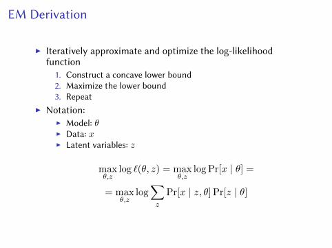
EM Derivation

I Iteratively approximate and optimize the log-likelihoodfunction1. Construct a concave lower bound2. Maximize the lower bound3. Repeat

I Notation:I Model: θI Data: xI Latent variables: z

maxθ,z

log `(θ, z) = maxθ,z

log Pr[x | θ] =

= maxθ,z

log∑z

Pr[x | z, θ] Pr[z | θ]

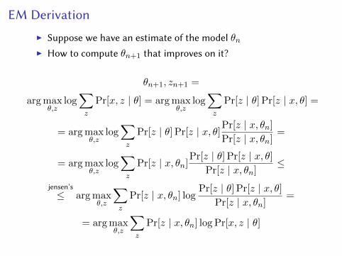
EM Derivation

I Suppose we have an estimate of the model θnI How to compute θn+1 that improves on it?

θn+1, zn+1 =

arg maxθ,z

log∑z

Pr[x, z | θ] = arg maxθ,z

log∑z

Pr[z | θ] Pr[z | x, θ] =

= arg maxθ,z

log∑z

Pr[z | θ] Pr[z | x, θ]Pr[z | x, θn]

Pr[z | x, θn]=

= arg maxθ,z

log∑z

Pr[z | x, θn]Pr[z | θ] Pr[z | x, θ]

Pr[z | x, θn]≤

jensen’s≤ arg max

θ,z

∑z

Pr[z | x, θn] logPr[z | θ] Pr[z | x, θ]

Pr[z | x, θn]=

= arg maxθ,z

∑z

Pr[z | x, θn] log Pr[x, z | θ]

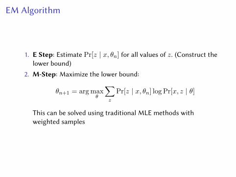
EM Algorithm

1. E Step: Estimate Pr[z | x, θn] for all values of z. (Construct thelower bound)

2. M-Step: Maximize the lower bound:

θn+1 = arg maxθ

∑z

Pr[z | x, θn] log Pr[x, z | θ]

This can be solved using traditional MLE methods withweighted samples

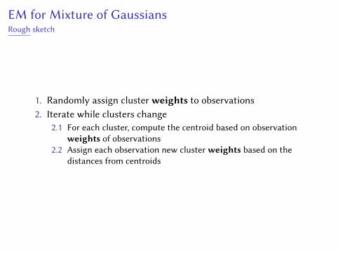
EM for Mixture of GaussiansRough sketch

1. Randomly assign cluster weights to observations2. Iterate while clusters change

2.1 For each cluster, compute the centroid based on observationweights of observations

2.2 Assign each observation new cluster weights based on thedistances from centroids

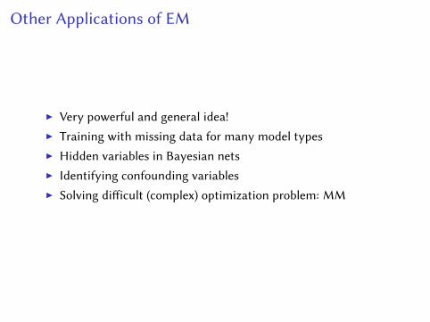
Other Applications of EM

I Very powerful and general idea!I Training with missing data for many model typesI Hidden variables in Bayesian netsI Identifying confounding variablesI Solving di�icult (complex) optimization problem: MM