Inverse Problems and Imaging doi:10.3934/ipi.xx.xx.xx

Volume X, No. 0X, 20xx, X–XX

GENERAL CONVERGENT EXPECTATION MAXIMIZATION

(EM)-TYPE ALGORITHMS FOR IMAGE RECONSTRUCTION

Ming Yan

Department of Mathematics

University of California, Los Angeles

Los Angeles, CA 90095, USA

Alex A.T. Bui

Department of Radiological Sciences

University of California, Los Angeles

Los Angeles, CA 90095, USA

Jason Cong

Department of Computer Sciences

University of California, Los Angeles

Los Angeles, CA 90095, USA

Luminita A. Vese

Department of MathematicsUniversity of California, Los Angeles

Los Angeles, CA 90095, USA

(Communicated by the associate editor name)

Abstract. Obtaining high quality images is very important in many areas of

applied sciences, such as medical imaging, optical microscopy, and astronomy.

Image reconstruction can be considered as solving the ill-posed and inverseproblem y = Ax+n, where x is the image to be reconstructed and n is the un-

known noise. In this paper, we propose general robust expectation maximiza-

tion (EM)-Type algorithms for image reconstruction. Both Poisson noise andGaussian noise types are considered. The EM-Type algorithms are performed

using iteratively EM (or SART for weighted Gaussian noise) and regularization

in the image domain. The convergence of these algorithms is proved in severalways: EM with a priori information and alternating minimization methods.To show the efficiency of EM-Type algorithms, the application in computerized

tomography reconstruction is chosen.

1. Introduction. Obtaining high quality images is very important in many areasof applied science, such as medical imaging, optical microscopy, and astronomy.For some applications such as positron-emission-tomography (PET) and computedtomography (CT), analytical methods for image reconstruction are available. For in-stance, filtered back projection (FBP) is the most commonly used method for imagereconstruction from CT by manufacturers of commercial imaging equipments [41].

2010 Mathematics Subject Classification. Primary: 90C30, 94A08; Secondary: 90C26, 92C55.Key words and phrases. Expectation maximization (EM), Richardson-Lucy, simultaneous alge-

braic reconstruction technique (SART), image reconstruction, total variation (TV), computerizedtomography.

This work is supported by the Center for Domain-Specific Computing (CDSC) funded by the

NSF Expedition in Computing Award CCF-0926127.

1 c©20xx American Institute of Mathematical Sciences

2 Ming Yan, Alex A.T. Bui, Jason Cong and Luminita A. Vese

However, it is sensitive to noise and suffers from streak artifacts (star artifacts). Analternative to this analytical reconstruction is the use of the iterative reconstructiontechnique, which is quite different from FBP. The main advantages of the iterativereconstruction technique over FBP are insensitivity to noise and flexibility [28].The data can be collected over any set of lines, the projections do not have to bedistributed uniformly in angle, and the projections can be even incomplete (limitedangle). With the help of parallel computing and graphics processing units (GPUs),even iterative methods can be solved very fast. Therefore, iterative methods be-come more and more important, and we will focus on the iterative reconstructiontechnique only.

The degradation model can be formulated as a linear inverse and ill-posed prob-lem:

(1) y = Ax+ b+ n.

Here, y is the measured data (vector in RM in the discrete case). A is a compactoperator (matrix in RM×N in the discrete case). For all the applications we willconsider, the entries of A are nonnegative and A does not have full column rank. xis the desired exact image (vector in RN in the discrete case). b is the backgroundemission and n is the noise (both are vectors in RM in the discrete case). We willconsider the case without background emission (b = 0) in this paper. Since thematrix A does not have full column rank, the computation of x directly by findingthe inverse of A is not reasonable because (1) is ill-posed and n is unknown. Evenfor the case without noise (n = 0), there are many solutions because A does nothave full column rank. When there is noise in the measured data (n 6= 0), findingx is more difficult because of the unknown n. Therefore regularization techniquesare needed for solving these problems efficiently.

One powerful technique for applying regularization is the Bayesian model, anda general Bayesian model for image reconstruction was proposed by Geman andGeman [15], and Grenander [18]. The idea is to use a priori information about theimage x to be reconstructed. In the Bayesian approach, we assume that measureddata y is a realization of a multi-valued random variable, denoted by Y and theimage x is also considered as a realization of another multi-valued random variable,denoted by X. Therefore, Bayes’ theorem gives us

(2) pX(x|y) =pY (y|x)pX(x)

pY (y).

This is a conditional probability of having X = x given that y is the measured data.After inserting the detected value y, we obtain a posterior probability distribution ofX. Then we can find x∗ such that pX(x|y) is maximized, as maximum a posteriori(MAP) likelihood estimation.

In general, X is assigned a Gibbs random field, which is a random variable withthe following probability distribution

(3) pX(x) ∼ e−βJ(x),

where J(x) is a given energy function (J(x) can be non-convex), and β is a positiveparameter. There are many different choices for J(x) depending on the applica-tions. Some examples are, for instance, quadratic penalization J(x) = ‖x‖22/2[12, 34], quadratic gradient J(x) = ‖∇x‖22/2 [54], total variation J(x) = ‖|∇x|‖1,and modified total variation [38, 40, 14, 6, 49, 51]. We also mention Good’s rough-ness penalization J(x) = ‖|∇x|2/x‖1 [26] for a slightly different regularization. We

Inverse Problems and Imaging Volume X, No. X (20xx), X–XX

General convergent EM-Type algorithms 3

assume here that ‖ · ‖1 and ‖ · ‖2 are the `1 and `2 norms respectively, and that ∇xdenotes the discrete gradient operator of an image x.

For the choices of probability densities pY (y|x), we can choose

(4) pY (y|x) ∼ e−‖Ax−y‖22/(2σ

2)

in the case of additive Gaussian noise, and the minimization of the negative log-likelihood function gives us the famous Tikhonov regularization method [46]

(5) minimizex

1

2‖Ax− y‖22 + βJ(x).

If the random variable Y of the detected values y follows a Poisson distribution[31, 42] with an expectation value provided by Ax instead of Gaussian distribution,we have

(6) yi ∼ Poisson(Ax)i, i.e., pY (y|x) ∼∏i

(Ax)yiiyi!

e−(Ax)i .

By minimizing the negative log-likelihood function, we obtain the following opti-mization problem

(7) minimizex≥0

∑i

((Ax)i − yi log(Ax)i

)+ βJ(x).

In this paper, we will focus on solving (5) and (7). It is easy to see that theobjective functions in (5) and (7) are convex if J(x) is a convex function. Addition-ally, with suitably chosen regularization J(x), the objective functions are strictlyconvex, and the solutions to these problems are unique. If J(x) = ‖|∇x|‖1, i.e,.the regularization is the total variation, the well-posedness of the regularizationproblems is shown in [1] and [6] for Gaussian and Poisson noise respectively. In thispaper, we also consider a more general case where J(x) is non-convex.

Relevant prior works are by Le et al. [31], Brune et al. [6, 7, 8], and Sidky etal. [44]. Additionally, we refer to Jia et al. [23], Jung et al. [27], Setzer et al. [39],Jafarpour et al. [22], Harmany et al. [19], Willet et al. [48], among other work. Wealso refer to the Compressive Sensing Resources [55]. The difference of this workfrom those will be discussed later.

The paper is organized as follows. In section 2, we will give a short introductionof expectation maximization (EM) iteration, or Richardson-Lucy algorithm, used inimage reconstruction without background emission from the view of optimization.In section 3, we will propose general EM-Type algorithms for image reconstructionwithout background emission when the measured data is corrupted by Poisson noise.This is based on the maximum a posteriori likelihood estimation and an EM step.In this section, these EM-Type algorithms are shown to be equivalent to EM algo-rithms with a priori information. In addition, these EM-Type algorithms are alsoconsidered as alternating minimization methods for equivalent optimization prob-lems, and the convergence results are obtained from both convex and non-convexJ(x). When the noise is weighted Gaussian noise, we also have the similar EM-Type algorithms. Simultaneous algebraic reconstruction technique is shown to beEM algorithm in section 4, and EM-Type algorithms for weighted Gaussian noiseare introduced in section 5. In section 5, we also show the convergence analysis ofEM-Type algorithms for weighted Gaussian noise via EM algorithms with a prioriinformation and alternating minimization methods. Some numerical experimentson image reconstruction are given in section 6 to show the efficiency of the EM-Typealgorithms. We will end this work by a short conclusion section.

Inverse Problems and Imaging Volume X, No. X (20xx), X–XX

4 Ming Yan, Alex A.T. Bui, Jason Cong and Luminita A. Vese

2. Expectation Maximization (EM) Iteration. A maximum likelihood (ML)method for image reconstruction based on Poisson data was introduced by Sheppand Vardi [42] in 1982 for image reconstruction in emission tomography. In fact,this algorithm was originally proposed by Richardson [37] in 1972 and Lucy [33] in1974 for image deblurring in astronomy. The ML method is a method for solvingthe special case of problem (7) without regularization term, i.e., J(x) is a constant,which means we do not have any a priori information about the image. Fromequation (6), for given measured data y, we have a function of x, the likelihood ofx, defined by pY (y|x). Then a ML estimation of the unknown image is defined asany maximizer x∗ of pY (y|x).

By taking the negative log-likelihood, one obtains, up to an additive constant,

f0(x) =∑i

((Ax)i − yi log(Ax)i

),

and the problem is to minimize this function f0(x) on the nonnegative orthant,because we have the constraint that the image x is nonnegative. In fact, we have

f(x) = DKL(y,Ax) :=∑i

(yi log

yi(Ax)i

+ (Ax)i − yi)

= f0(x) + C,

where DKL(y,Ax) is the Kullback-Leibler (KL) divergence of Ax from y, and Cis a constant independent of x. The KL divergence is considered as a data-fidelityfunction for Poisson data just like the standard least-square ‖Ax− y‖22 is the data-fidelity function for additive Gaussian noise. DKL(y, ·) is convex, nonnegative andcoercive on the nonnegative orthant, so the minimizers exist and are global.

In order to find a minimizer of f(x) with the constraint xj ≥ 0 for all j, we cansolve the Karush-Kuhn-Tucker (KKT) conditions [30, 29],∑

i

(Ai,j(1−

yi(Ax)i

)

)− sj = 0, j = 1, · · · , N,

sj ≥ 0, xj ≥ 0, j = 1, · · · , N,sTx = 0,

where sj is the Lagrange multiplier corresponding to the constraint xj ≥ 0. By thepositivity of xj, sj and the complementary slackness condition sTx = 0, wehave sjxj = 0 for every j ∈ 1, · · · , N. Multiplying by xj gives us∑

i

(Ai,j(1−

yi(Ax)i

)

)xj = 0, j = 1, · · · , N.

Therefore, we have the following iteration scheme

(8) xk+1j =

∑i

(Ai,j(

yi(Axk)i

))

∑i

Ai,jxkj .

This is the well-known EM iteration or Richardson-Lucy algorithm in image recon-struction, and an important property of it is that it preserves positivity. If xk ispositive, then xk+1 is also positive if A preserves positivity. It is also shown thatfor each iteration,

∑i

(Ax)i is fixed and equals∑i

yi. Since∑i

(Ax)i =∑j

(∑i

Ai,j)xj ,

the minimizer has a weighted l1 constraint.Shepp and Vardi showed in [42] that this is equivalent to the EM algorithm

proposed by Dempster, Laird and Rubin [13]. To make it clear, EM iteration

Inverse Problems and Imaging Volume X, No. X (20xx), X–XX

General convergent EM-Type algorithms 5

means the special EM method used in image reconstruction, while EM algorithmmeans the general EM algorithm for solving missing data problems.

3. EM-Type Algorithms for Poisson data. The method shown in the lastsection is also called maximum-likelihood expectation maximization (ML-EM) re-construction, because it is a maximum likelihood approach without any Bayesianassumption on the images. If additional a priori information about the image isgiven, we have maximum a posteriori probability (MAP) approach [21, 32], whichis the case with regularization term J(x). Again we assume here that the detecteddata is corrupted by Poisson noise, and the regularization problem is

minimizex

EP (x) := βJ(x) +∑i

((Ax)i − yi log(Ax)i) ,

subject to xj ≥ 0, j = 1, · · · , N.(9)

This is still a convex constraint optimization problem if J is convex and we can findthe optimal solution by solving the KKT conditions:

β∂J(x)j +∑i

(Ai,j(1−

yi(Ax)i

)

)− sj = 0, j = 1, · · · , N,

sj ≥ 0, xj ≥ 0, j = 1, · · · , N,sTx = 0.

Here sj is the Lagrangian multiplier corresponding to the constraint xj ≥ 0. Bythe positivity of xj, sj and the complementary slackness condition sTx = 0,we have sjxj = 0 for every j ∈ 1, · · · , N. Thus we obtain

βxj∂J(x)j +∑i

(Ai,j(1−

yi(Ax)i

)

)xj = 0, j = 1, · · · , N,

or equivalently

βxj∑

i

Ai,j∂J(x)j + xj −

∑i

(Ai,j(

yi(Ax)i

))

∑i

Ai,jxj = 0, j = 1, · · · , N.

Notice that the last term on the left hand side is an EM step (8). After pluggingthe EM step into the equation, we obtain

(10) βxj∑

i

Ai,j∂J(x)j + xj − xEMj = 0, j = 1, · · · , N,

which is the optimality condition for the following optimization problem

(11) minimizex

EP1 (x, xEM ) := βJ(x) +∑j

(∑i

Ai,j)(xj − xEMj log xj

).

Therefore we propose the general EM-Type algorithms in Algorithm 1. Theinitial guess x0 can be any positive initial image, and ε, chosen for the stoppingcriteria, is a small constant. Num Iter is the maximum number of iterations. IfJ(x) is constant, the second step is just xk = xk−

12 and this is exactly the ML-

EM from the previous section. When J(x) is not constant, we have to solve anoptimization problem at each iteration. In general, the problem can not be solvedanalytically, and we have to use iterative methods to solve it. However, in practice,we do not have to solve it exactly to the steady state, just a few iterations are

Inverse Problems and Imaging Volume X, No. X (20xx), X–XX

6 Ming Yan, Alex A.T. Bui, Jason Cong and Luminita A. Vese

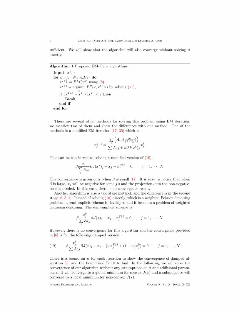
sufficient. We will show that the algorithm will also converge without solving itexactly.

Algorithm 1 Proposed EM-Type algorithms.

Input: x0, εfor k = 0 : Num Iter do

xk+ 12 = EM(xk) using (8),

xk+1 = argminx

EP1 (x, xk+ 12 ) by solving (11),

if ‖xk+1 − xk‖/‖xk‖ < ε thenBreak,

end ifend for

There are several other methods for solving this problem using EM iteration,we mention two of them and show the differences with our method. One of themethods is a modified EM iteration [17, 35] which is

xk+1j =

∑i

(Ai,j(

yi(Axk)i

))

∑i

Ai,j + β∂J(xk)jxkj .

This can be considered as solving a modified version of (10):

βxj∑

i

Ai,j∂J(xk)j + xj − xEMj = 0, j = 1, · · · , N.

The convergence is given only when β is small [17]. It is easy to notice that whenβ is large, xj will be negative for some j’s and the projection onto the non-negativecone is needed. In this case, there is no convergence result.

Another algorithm is also a two stage method, and the difference is in the secondstage [6, 8, 7]. Instead of solving (10) directly, which is a weighted Poisson denoisingproblem, a semi-implicit scheme is developed and it becomes a problem of weightedGaussian denoising. The semi-implicit scheme is

βxkj∑

i

Ai,j∂J(x)j + xj − xEMj = 0, j = 1, · · · , N.

However, there is no convergence for this algorithm and the convergence providedin [6] is for the following damped version:

(12) βxkj∑

i

Ai,j∂J(x)j + xj − (wxEMj + (1− w)xkj ) = 0, j = 1, · · · , N.

There is a bound on w for each iteration to show the convergence of damped al-gorithm [6], and the bound is difficult to find. In the following, we will show theconvergence of our algorithm without any assumptions on β and additional param-eters. It will converge to a global minimum for convex J(x) and a subsequence willconverge to a local minimum for non-convex J(x).

Inverse Problems and Imaging Volume X, No. X (20xx), X–XX

General convergent EM-Type algorithms 7

3.1. Equivalence to EM Algorithms with a priori Information. In thissubsection, the EM-Type algorithms are shown to be equivalent to EM algorithmswith a priori information. The EM algorithm is a general approach for maximizing aposterior distribution when some of the data is missing [13]. It is an iterative methodwhich alternates between expectation (E) steps and maximization (M) steps. Forimage reconstruction, we assume that the missing data is the latent variables zij,describing the intensity of pixel (or voxel) j observed by detector i. It is introducedas a realization of a multi-valued random variable Z, and for each (i, j) pair, zijfollows a Poisson distribution with expected value Ai,jxj . Then the observed datais yi =

∑j

zij , because the summation of two Poisson distributed random variables

also follows a Poisson distribution, whose expected value is the summation of thetwo expected values.

The original E-step is to find the expectation of the log-likelihood given thepresent variables xk:

Q(x|xk) = Ez|xk,y log p(x, z|y).

Then, the M-step is to choose xk+1 to maximize the expected log-likelihood Q(x|xk)found in the E-step:

xk+1 = argmaxx

Ez|xk,y log p(x, z|y) = argmaxx

Ez|xk,y log(p(y, z|x)p(x))

= argmaxx

Ez|xk,y

∑ij

(zij log(Ai,jxj)−Ai,jxj)− βJ(x)

= argminx

∑ij

(Ai,jxj − Ez|xk,yzij log(Ai,jxj)) + βJ(x).

(13)

From (13), what we need before solving it is just Ez|xk,yzij. Therefore we can

compute the expectation of missing data zij given present xk and the conditionyi =

∑j

zij , denoting this as an E-step. Because for fixed i, zij are Poisson

variables with mean Ai,jxkj and∑j

zij = yi, the conditional distribution of zij

is the binomial distribution

(yi,

Ai,jxkj

(Axk)i

). Thus we can find the expectation of zij

with all these conditions by the following E-step

(14) zk+1ij = Ez|xk,yzij =

Ai,jxkj yi

(Axk)i.

After obtaining the expectation for all zij , we can solve the M-step (13).We will show that EM-Type algorithms are exactly the described EM algorithms

with a priori information. Recalling the definition of xEM , we have

xEMj =

∑i

zk+1ij∑

i

Ai,j.

Therefore, the M-step is equivalent to

xk+1 = argminx

∑ij

(Ai,jxj − zk+1ij log(Ai,jxj)) + βJ(x)

= argminx

∑j

(∑i

Ai,j)(xj − xEMj log(xj)) + βJ(x).

Inverse Problems and Imaging Volume X, No. X (20xx), X–XX

8 Ming Yan, Alex A.T. Bui, Jason Cong and Luminita A. Vese

We have shown that EM-Type algorithms are EM algorithms with a priori informa-tion. The convergence of EM-Type algorithms is shown in the next subsection fromthe equivalence of EM-Type algorithms with alternating minimization methods forequivalent problems.

3.2. EM-Type Algorithms are Alternating Minimization Methods. In thissection, we will show that these algorithms can also be derived from alternating min-imization methods of other problems with variables x and z. The new optimizationproblems are

minimizex,z

EP (x, z) :=∑ij

(zij log

zijAi,jxj

+Ai,jxj − zij)

+ βJ(x),

subject to∑j

zij = yi, i = 1, · · · ,M,

zij ≥ 0, i = 1, · · · ,M, j = 1, · · · , N.

(15)

Here EP is used again to define the new function. EP (·) means the negative log-likelihood function of x, while EP (·, ·) means the new function of x and z definedin new optimization problems. x ≥ 0 is implicitly included in the formula.

Having initial guess x0, z0 of x and z, the iteration for k = 0, 1, · · · is as follows:

zk+1 = argminz

EP (xk, z), subject to∑j

zij = yi,

xk+1 = argminx

EP (x, zk+1).

Firstly, in order to obtain zk+1, we fix x = xk and easily derive

(16) zk+1ij =

Ai,jxkj yi

(Axk)i.

After finding zk+1, let z = zk+1 fixed and update x, then we have

xk+1 = argminx

∑ij

(Ai,jxj + zk+1

ij logzk+1ij

Ai,jxj

)+ βJ(x)

= argminx

∑ij

(Ai,jxj − zk+1

ij log(Ai,jxj))

+ βJ(x),

which is the M-Step (13) in section 3.1. Thus EM-Type algorithms for (9) arealternating minimization methods for problem (15). The equivalence of problems(9) and (15) is provided in the following theorem.

Theorem 3.1. If (x∗, z∗) is a local minimum of problem (15), then x∗ is also alocal minimum of (9). If x∗ is a local minimum of (9), then we can find z∗ from(16) and (x∗, z∗) is a local minimum of problem (15).

Proof. If (x∗, z∗) is a local minimum of problem (15), we can find δ > 0 so thatfor all (x, z) such that ‖(x − x∗, z − z∗)‖ < δ and

∑j zij = yi, zij ≥ 0, the expres-

sion EP (x, z) ≥ EP (x∗, z∗) holds. Let us assume that x∗ is not a local minimumof problem (9), then there exist a sequence xk such that limk→∞ xk = x∗ andEP (xk) < EP (x∗). Let zk+1 be chosen from (16) for corresponding xk and we haveEP (xk, zk+1) = EP (xk) < EP (x∗) = EP (x∗, z∗), and limk→∞ zk = z∗. This is acontradiction with that (x∗, z∗) is a local minimum of (15).

Inverse Problems and Imaging Volume X, No. X (20xx), X–XX

General convergent EM-Type algorithms 9

In another way, if x∗ is a local minimum of (9), there exist a δ > 0 such thatfor all x such that ‖x − x∗‖ ≤ δ and x ≥ 0, we have EP (x) ≥ EP (x∗). If wechoose (x, z) such that ‖(x − x∗, z − z∗)‖ < δ and

∑j zij = yi, then we have

EP (x, z) ≥ EP (x) ≥ EP (x∗) = EP (x∗, z∗). Thus (x∗, z∗) is a local minimum ofproblem (15).

From the equivalence of EM-Type algorithm with alternating minimization meth-ods, we know that the function value is decreasing. Next, we will show that if J(x)is convex, (xk, zk) will converge to a global minimum of problem (15), and if J(x) isnon-convex, a subsequence of (xk, zk) will converge to a local minimum of prob-lem (15). Before that, we show two lemmas which are used in the proof of theconvergence results.

For s > 0, t ≥ 0, let us define dP (s, t) = t log ts + s− t, assuming that 0 log 0 = 0

and log 0 = −∞. In addition Z is defined as Z := z : zij ≥ 0,∑j zij = yi. We

will have the following lemmas:

Lemma 3.2. For all p > 0, s > 0, t ≥ 0, we have

(17) dP (s, t)− dP (p, t) + dP (p, s) = logs

p(s− t).

Proof.

dP (s, t)− dP (p, t) + dP (p, s)

=t logt

s+ s− t−

(t log

t

p+ p− t

)+

(s log

s

p+ p− s

)= log

s

p(s− t).

Lemma 3.3. For all p > 0, q ≥ 0, s > 0, t ≥ 0, we have

(18) dP (s, t)− dP (p, t) + dP (q, t)− p− qp

(s− p) ≥ 0.

Proof. Since dP (s, t) is convex for (s, t) : s > 0, t ≥ 0, we have

ddP ((s, t), (p, q))

:=dP (s, t)− dP (p, q)−∇pdP (p, q)(s− p)−∇qdP (p, q)(t− q)

=dP (s, t)− dP (p, q)−(−qp

+ 1

)(s− p)− log

q

p(t− q)

=dP (s, t)− dP (p, q)− p− qp

(s− p)− dP (p, t) + dP (q, t) + dP (p, q).

(19)

The last equality comes form Lemma 3.2. Since dP (s, t) is convex, the result followsbecause ddP ((s, t), (p, q)) ≥ 0.

In order to show the convergence for general J(x), we will need the followingassumption on J(x).

Assumption 1. J(x) is lower semicontinuity, bounded below, and there existsδ > 0 for any given z ∈ Z and any local minimum point x of EP (x, z), such thatfor all x satisfying ‖x− x‖ ≤ δ, the following inequality holds:

βJ(x) ≥ βJ(x)−∑ij

Ai,j xj − zijAi,j xj

Ai,j(xj − xj)−∑ij

ddP ((Ai,jxj , zij), (Ai,j xj , zij)),

Inverse Problems and Imaging Volume X, No. X (20xx), X–XX

10 Ming Yan, Alex A.T. Bui, Jason Cong and Luminita A. Vese

where z ∈ Z.

Remark 1. For convex J(x), we have a stronger statement

(20) βJ(x) ≥ βJ(x)− 〈∂xJ(x), x− x〉 = βJ(x)−∑ij

Ai,j xj − zijAi,j xj

Ai,j(xj − xj).

The equality comes from the optimality condition for x.

With Assumption 1, we have the following theorem which will provide an alter-native way to determine the local optimality.

Theorem 3.4. If there exists (x, z) such that z = argmin z EP (x, z) and x is a

local minimum point of EP (x, z). Then (x, z) is a local minimum of problem (15).

Proof. Since x is a local minimum point of EP (x, z), there exists δ > 0 such thatfor all x satisfying ‖x− x‖ ≤ δ, we have, from Assumption 1, that

βJ(x)

≥βJ(x)−∑ij

Ai,j xj − zijAi,j xj

Ai,j(xj − xj)−∑ij

ddP ((Ai,jxj , zij), (Ai,j xj , zij))

=βJ(x) +∑ij

dP (Ai,j xj , zij)−∑ij

dP (Ai,jxj , zij) +∑ij

logzij

Ai,j xj(zij − zij)

=βJ(x) +∑ij

dP (Ai,j xj , zij)−∑ij

dP (Ai,jxj , zij),

for all z ∈ Z. The first equality comes from (19), and the second equality holdsbecause for any z ∈ Z, we have∑

ij

logzij

Ai,j xj(zij − zij) =

∑i

logyi

(Ax)i

∑j

(zij − zij) = 0.

Therefore, we have

EP (x, z) = βJ(x) +∑ij

dP (Ai,jxj , zij) ≥ βJ(x) +∑ij

dP (Ai,j xj , zij) = EP (x, z)

for all x satisfying ‖x − x‖ ≤ δ and z ∈ Z, which means that (x, z) is a localminimum of problem (15).

Remark 2. In fact, (x, z) being a local minimum of problem (15) requires thatthere exist a constant δ > 0 such that for all x satisfying ‖x− x‖ ≤ δ, the followinginequality holds:

βJ(x) ≥ βJ(x)−∑ij

Ai,j xj − zijAi,j xj

Ai,j(xj − xj)−∑ij

ddP ((Ai,jxj , zij), (Ai,j xj , zij)),

where z ∈ Z. Therefore, it is reasonable to make the assumptions on J(x).

Theorem 3.5. The algorithm will converge to a global minimum of problem (15)for convex J(x), and there exists a subsequence which converges to a local minimumof problem (15) for non-convex J(x).

Inverse Problems and Imaging Volume X, No. X (20xx), X–XX

General convergent EM-Type algorithms 11

Proof. From previous theorem, we have to show that it converges to (x∗, z∗) withz∗ = argmin z E

P (x∗, z) and x∗ being a local minimum point of EP (x, z∗).∑ij

dP (Ai,jxj , zij) +∑ij

dP (zkij , zij)

(18)=∑ij

dP (Ai,jxkj , zij) +

∑ij

zkij −Ai,jxkjAi,jxkj

(Ai,jx

kj −Ai,jxj

)+ ddP ((Ai,jxj , zij), (Ai,jx

kj , z

kij))

(17)=∑ij

dP (zk+1ij , zij) +

∑ij

dP (Ai,jxkj , z

k+1ij ) +

∑ij

logAi,jx

kj

zk+1ij

(zk+1ij − zij)

+∑ij

zkij −Ai,jxkjAi,jxkj

(Ai,jx

kj −Ai,jxj

)+ ddP ((Ai,jxj , zij), (Ai,jx

kj , z

kij))

=∑ij

dP (zk+1ij , zij) +

∑ij

dP (Ai,jxkj , z

k+1ij ) + βJ(xk)− βJ(x)

+∑ij

zkij −Ai,jxkjAi,jxkj

(Ai,jx

kj −Ai,jxj

)+ βJ(x)− βJ(xk)

+ ddP ((Ai,jxj , zij), (Ai,jxkj , z

kij))

≥∑ij

dP (zk+1ij , zij) +

∑ij

dP (Ai,jxkj , z

k+1ij ) + βJ(xk)− βJ(x).

(21)

The last inequality comes from Assumption 1, and it holds only for x close to xk.Therefore, we have

∑ij d

P (zkij , zij)−∑ij d

P (zk+1ij , zij) ≥ EP (xk, zk+1)−EP (x, z).

Since J(x) is bounded below and dP (+∞, z) = +∞, xk is bounded and there existsa subsequence denoted by xok converging to x∗. Let z∗ = argmin z E

P (x∗, z).Then we have limk→∞ zok+1 = z∗ and EP (x∗, z∗) ≤ limk→∞EP (xok , zok+1) ≤EP (xok , zok+1). Since EP (xk, zk+1) is decreasing, we have EP (x∗, z∗) < EP (xk, zk)and limk→∞EP (xk, zk) = EP (x∗, z∗). From (21), dP (zkij , z

∗ij) is monotone decreas-

ing and zok is bounded, there exists a subsequence converging to z, and westill denote it by zok for simplicity. Since EP (x∗, z) ≤ limk→∞EP (xok , zok) =EP (x∗, z∗), we have z = z∗. Next, we will show that x∗ is a local minimum pointof EP (x, z∗). From Assumption 1 we have

βJ(x) ≥βJ(xok)−∑ij

Ai,jxokj − z

okij

Ai,jxokj

Ai,j(xj − xokj )

−∑ij

ddP ((Ai,jxj , zokij ), (Ai,jx

okj , z

okij ))

=βJ(xok)−∑ij

dP (Ai,jxj , zokij ) +

∑ij

dP (Ai,jxokj , z

okij ).

Let k → ∞ we have βJ(x) +∑ij d

P (Ai,jxj , z∗ij) ≥ βJ(x∗) +

∑ij d

P (Ai,jx∗j , z∗ij),

which means that x∗ is a local minimum of EP (x, z∗) and (x∗, z∗) is a local mini-mum.

If J(x) is convex, we can choose (x, z) in (21) to be a global minimum (x, z),and we have that dP (zkij , zij) is monotone decreasing. Thus z is bounded and foreach convergent subsequence of zok with limk→∞ zok = z, we can find xok and

Inverse Problems and Imaging Volume X, No. X (20xx), X–XX

12 Ming Yan, Alex A.T. Bui, Jason Cong and Luminita A. Vese

limk→∞ xok = x, with x being a minimum point of EP (x, z). We have EP (x, z) ≤limk→∞EP (xok , zok) = EP (x, z). Thus (x, z) is also a global minimum. Therefore,limk→∞ zk = z∗, and let x∗ = argmin xE

P (x, z∗) satisfying limk→∞ xk = x∗. Theresulting (x∗, z∗) is a global minimum of problem (15).

Remark 3. Even if the second step is not solved exactly, we have EP (xk+1) <EP (xk) if EP (xk+1, zk+1) < EP (xk, zk+1). In fact it is impossible to solve thesecond step exactly in many cases, and we have to approximately solve it usingiterative methods.

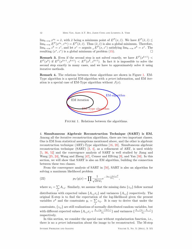
Remark 4. The relations between these algorithms are shown in Figure 1. EM-Type algorithm is a special EM-algorithm with a priori information, and EM iter-ation is a special case of EM-Type algorithm without J(x).

EM-algorithm

EM-Type algorithm

EM iteration

Figure 1. Relations between the algorithms.

4. Simultaneous Algebraic Reconstruction Technique (SART) is EM.Among all the iterative reconstruction algorithms, there are two important classes.One is EM from statistical assumptions mentioned above, and the other is algebraicreconstruction technique (ART)-Type algorithms [16, 20]. Simultaneous algebraicreconstruction technique (SART) [3, 4], as a refinement of ART, is used widely[5, 36, 52] and the convergence analysis of SART is well studied by Jiang andWang [25, 24], Wang and Zheng [47], Censor and Elfving [9], and Yan [50]. In thissection, we will show that SART is also an EM algorithm, building the connectionbetween these two classes.

From the convergence analysis of SART in [50], SART is also an algorithm forsolving a maximum likelihood problem

(22) pY (y|x) =∏i

1√2πwi

e− (yi−(Ax)i)

2

2wi ,

where wi =∑j

Ai,j . Similarly, we assume that the missing data zij follow normal

distributions with expected values Ai,jxj and variances Ai,j respectively. Theoriginal E-step is to find the expectation of the log-likelihood given the presentvariables xk and the constraints yi =

∑j

zij . It is easy to derive that under the

constraints, zij are still realizations of normally distributed random variables, but

with different expected values Ai,jxj+Ai,j(yi−(Ax)i)

wi and variances Ai,j(wi−Ai,j)

wi

respectively.In this section, we consider the special case without regularization function, i.e.,

there is no a priori information about the image to be reconstructed. The M-step

Inverse Problems and Imaging Volume X, No. X (20xx), X–XX

General convergent EM-Type algorithms 13

is to maximize the expected value of the log-likelihood function,

Ez|xk,y log p(y, z|x) = −Ez|xk,y

∑ij

(zij −Ai,jxj)2

2Ai,j+ C

= −∑ij

(Ez|xk,yzij −Ai,jxj)2

2Ai,j+ C,

where C is a constant independent of x and z. Therefore, for the E-step we haveto just find the expected value of zij given xk and the constraints, which is

zk+1ij = Ai,jx

kj +

Ai,j(yi − (Axk)i)

wi.

For the M-step, we find xk+1 by maximizing p(y, zk+1|x) with respect to x, whichhas an analytical solution

(23) xk+1j =

∑i

zk+1ij∑

i

Ai,j= xkj +

1∑i

Ai,j

∑i

Ai,j(yi − (Axk)i)

wi.

This is the original SART algorithm proposed by Andersen [3].From the convergence analysis of SART in [50], the result of SART depends on

the initialization x0 for both noiseless and noisy cases when A is underdetermined.

Remark 5. SART is just one example of Landweber-like schemes for solving sys-tems of linear equations. By changing the variance of yi and zij , different schemescan be proposed. For other Landweber-like schemes such as component averagingin [9, 10], they can also be derived from the EM algorithm similarly by choosingdifferent variances. Furthermore, new schemes can be derived by choosing differentvariances.

5. EM-Type Algorithms for Gaussian Noise. It is shown in the last sectionthat SART is an EM algorithm based on weighted Gaussian assumption for theproblem without regularization. Without regularization, the original problem isill-posed, and the result will depend on the initialization x0. In this section, we willconsider the regularized problem

(24) minimizex

EG(x) := βJ(x) +∑i

((Ax)i − yi)2

2wi,

and derive EM-Type algorithms with Gaussian noise assumption for solving it. TheE-step is the same as in the case without regularization,

(25) zk+1ij = Ai,jx

kj +

Ai,j(yi − (Axk)i)

wi.

However, the M-step is different because we have a priori information on the image xto be reconstructed. The new M-step is to solve the following optimization problems

(26) minimizex

∑ij

(zk+1ij −Ai,jxj)2

2Ai,j+ βJ(x),

Inverse Problems and Imaging Volume X, No. X (20xx), X–XX

14 Ming Yan, Alex A.T. Bui, Jason Cong and Luminita A. Vese

which is equivalent to

minimizex

1

2

∑j

(∑i

Ai,j)(xj −

∑i

zk+1ij∑

i

Ai,j)2 + βJ(x).

From the SART iteration (23) in the last section, we can define

(27) xSART = xkj +1∑

i

Ai,j

∑i

Ai,j(yi − (Axk)i)

wi.

and have

(28) xk+1 = argminx

EG1 (x, xSART ) :=1

2

∑j

(∑i

Ai,j)(xj − xSARTj )2 + βJ(x).

Therefore, the proposed EM-Type algorithms for image reconstruction with Gauss-ian noise are as follows.

Algorithm 2 Proposed EM-Type algorithms for Gaussian noise.

Input: x0, ε,for k = 0 : Num Iter do

xk+ 12 = SART (xk) using (27)

xk+1 = argmin EG1 (x, xk+ 12 ) by solving (28)

if ‖xk+1 − xk‖/‖xk‖ < ε thenBreak,

end ifend for

The initial guess x0 can be any initial image and ε, chosen for the stoppingcriteria, is very small. Num Iter is the maximum number of iterations. WhenJ(x) is not constant, we have to solve an optimization problem for each iteration.The convergence analysis of these algorithms can be shown similarly as for the casewith Poisson noise, which is described in the following subsection.

5.1. EM-Type Algorithms are Alternating Minimization Methods. Sameas the algorithms for Poisson data, the algorithms can also be derived from analternating minimization method of other problems with variables x and z. Thenew problems are

minimizex,z

EG(x, z) :=∑ij

(zij −Ai,jxj)2

2Ai,j+ βJ(x),

subject to∑j

zij = yi, i = 1, · · ·M.(29)

Here EG is used again to define the new function. EG(·) means the negative log-likelihood function of x, while EG(·, ·) means the new function of x and z definedin new optimization problems. The iteration is as follows:

zk+1 = argminz

E(xk, z), subject to∑j

zij = yi.

xk+1 = argminx

E(x, zk+1).

Inverse Problems and Imaging Volume X, No. X (20xx), X–XX

General convergent EM-Type algorithms 15

First, let us fix x = xk and update z. It is easy to derive

zk+1ij = Ai,jx

kj +

Ai,jwi

(yi − (Axk)i

).

Then, by fixing z = zk+1 and updating x, we have

xk+1 = argminx

∑ij

(zij −Ai,jxj)2

2Ai,j+ βJ(x)

= argminx

1

2

∑j

(∑i

Ai,j)(xj −

∑i

zij

2∑i

Ai,j)2 + βJ(x).

If J(x) is convex, problem (29) is convex, and we can find the minimizer withrespect to z for fixed x first and obtain a function of x as follows,∑

i

((Ax)i − yi)2

2wi+ βJ(x),

which is also convex and equals EG(x). Therefore EM-Type algorithms will con-verge to the solution of (24).

The convergence can be shown similarly with small changes in the definition ofdP (s, t), for weighed Gaussian noise, we can define dG(s, t) = 1

2 (s− t)2. In additionZ is defined as Z := z : zij = 0 if Ai,j = 0,

∑j zij = yi. The corresponding

lemmas are provided without proof.

Lemma 5.1. For all p, s, t ∈ R, we have

dG(s, t)− dG(p, t) + dG(p, s) = (s− p)(s− t).

Lemma 5.2. For all p, q, s, t ∈ R, we have

ddG((s, t), (p, q)) := dG(s, t)− dG(p, t) + dG(q, t)− (p− q)(s− p) ≥ 0.

As for the Poisson noise case, we have the following assumption on J(x).

Assumption 2. J(x) is lower semicontinuity, bounded below, and there existsδ > 0 for any given z ∈ Z and any local minimum point x of EG(x, z), such thatfor all x satisfying ‖x− x‖ ≤ δ, the following inequality holds:

βJ(x) ≥βJ(x)−∑ij

1

Ai,j(Ai,j xj − zij)Ai,j(xj − xj)

−∑ij

1

Ai,jddG((Ai,jxj , zij), (Ai,j xj , zij)),

where z ∈ Z.

Remark 6. For convex J(x), we have a stronger statement

βJ(x) ≥ βJ(x)− 〈∂xJ(x), x− x〉 = βJ(x)−∑ij

1

Ai,j(Ai,j xj − zij)Ai,j(xj − xj).

The equality comes from the optimality condition for x.

With this assumption, we have the following theorem which will provide analternative way to determine the local optimality. The proof is similar to the caseof Poisson noise and we omit it here.

Inverse Problems and Imaging Volume X, No. X (20xx), X–XX

16 Ming Yan, Alex A.T. Bui, Jason Cong and Luminita A. Vese

Theorem 5.3. If there exists (x, z) such that z = argmin z EG(x, z) and x is a

local minimum point of EG(x, z). Then (x, z) is a local minimum of problem (29).

The convergence result is similar and we put it here without proof.

Theorem 5.4. The algorithm will converge to a global minimum of problem (29)for convex J(x), and there exists a subsequence which converges to a local minimumof problem (29) for non-convex J(x).

5.2. Relaxation. In practice, some authors use a relaxation of SART reconstruc-tion, which is

xk+1j = xkj +

w∑i

Ai,j

∑i

Ai,j(yi − (Axk)i)

wi,

with a relaxant coefficient w. The convergence of this relaxation is shown in [25,24, 50] for any w ∈ (0, 2). Inspired by this strategy, we have a relaxation of theEM-Type algorithms for image reconstruction with Gaussian noise. The EM-stepis the relaxed SART with relaxant coefficient w:

xk+ 1

2j = xkj +

w∑i

Ai,j

∑i

Ai,j(yi − (Axk)i)

wi.

The corresponding regularization step is

xk+1 = argminx

1

2

∑j

(∑i

Ai,j)(xj − xk+ 1

2j )2 + wβJ(x).

When w = 1, we have already discussed the convergence in the previous subsectionsby EM algorithms with a priori information and alternating minimization methods.For w 6= 1, we will show the convergence of the relaxed EM-Type algorithms forw ∈ (0, 1) by alternating minimization methods.

We will show that the relaxed EM-Type algorithms are equivalent to solving theunconstrained problems

(30) minimizex,z

EGR (x, z) :=∑ij

(zij −Ai,jxj)2

2Ai,j+ γ

∑i

(∑j zij − yi)2

2wi+ wβJ(x),

where γ = w1−w , by alternating minimization between x and z. First, fix x = xk,

we can solve the problem of z only, and the analytical solution is

(31) zk+1ij = Ai,jx

kj +

γ

1 + γ

Ai,jwi

(yi − (Axk)i

)= Ai,jx

kj + w

Ai,jwi

(yi − (Axk)i

).

Then let z = zk+1 fixed, and we can find xk+1 by solving

minimizex

∑ij

(zij −Ai,jxj)2

2Ai,j+ wβJ(x)

=1

2

∑j

(∑i

Ai,j)(xj −

∑i

zij∑i

Ai,j)2 + wβJ(x) + C,

where C is a constant independent of x. Having zk+1 from (31), we can calculate∑i

zk+1ij∑

i

Ai,j= xkj +

w∑i

Ai,j

∑i

Ai,j(yi − (Axk)i)

wi= x

k+ 12

j .

Inverse Problems and Imaging Volume X, No. X (20xx), X–XX

General convergent EM-Type algorithms 17

Therefore this relaxed EM-Type algorithm is an alternating minimization method.We will show next that the result of this relaxed EM-Type algorithm is the solutionto (24).

Because the objective function EGR (x, z) in (30) is convex if J(x) is convex, wecan first minimize the function with respect to z with x fixed. Then the problembecomes

minimizex

γ

1 + γ

∑i

((Ax)i − yi)2

2wi+ wβJ(x)

= w∑i

((Ax)i − yi)2

2wi+ wβJ(x).

We have shown in this subsection that the relaxed EM-Type algorithm will alsoconverge to the solution of the original problem (24) when α ∈ (0, 1].

6. Numerical Experiments. As mentioned in the introduction, the main focusof this paper is the convergence result of EM-Type algorithms, and some of thenumerical experiments in this section have been included in [49, 51]. The newlyadded experiment is using of a non-convex J(x). In addition, this algorithm hasbeen implemented in different hardwares and the speedups can be found in [11].

In this section, several numerical experiments are provided to show the efficiencyof EM-Type algorithms. Though these EM-Type algorithms can be used in manyapplications, we choose Computed Tomography (CT) image reconstruction as ourapplication in this work. CT is a medical imaging method which utilizes X-rayequipment to produce a two dimensional (or three dimensional) image of the insideof an object from a large series of one dimensional (or two dimensional) X-rayimages taken along a single axis of rotation [20]. In CT reconstruction, the operatorA is the discrete Radon transform, and the discrete version of A is constructed bySiddon’s algorithm [43, 53]. The problem is to reconstruct the image from themeasurements, which is equivalent to solve Ax = b. Poisson noise is assumed [45]and two regularizations are used: the total variation (TV), and an approximationto a non-convex Mumford-Shah TV-like version.

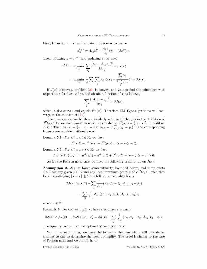
6.1. CT Reconstruction using EM+TV (2D). At first, we illustrate one method(EM+TV) on a simple synthetic object (two dimensional Shepp-Logan phantom),see Figure 2.

Original x

Figure 2. 2D Shepp-Logan phantom

The most common method used in commercial CT (computerized tomography) isthe filtered back projection (FBP), which can be implemented in a straight forward

Inverse Problems and Imaging Volume X, No. X (20xx), X–XX

18 Ming Yan, Alex A.T. Bui, Jason Cong and Luminita A. Vese

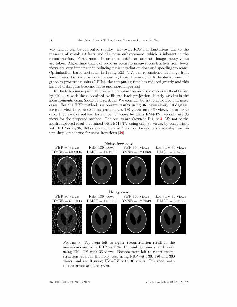
way and it can be computed rapidly. However, FBP has limitations due to thepresence of streak artifacts and the noise enhancement, which is inherent in thereconstruction. Furthermore, in order to obtain an accurate image, many viewsare taken. Algorithms that can perform accurate image reconstruction from fewerviews are very important in reducing patient radiation dose and speeding up scans.Optimization based methods, including EM+TV, can reconstruct an image fromfewer views, but require more computing time. However, with the development ofgraphics processing units (GPUs), the computing time has reduced greatly and thiskind of techniques becomes more and more important.

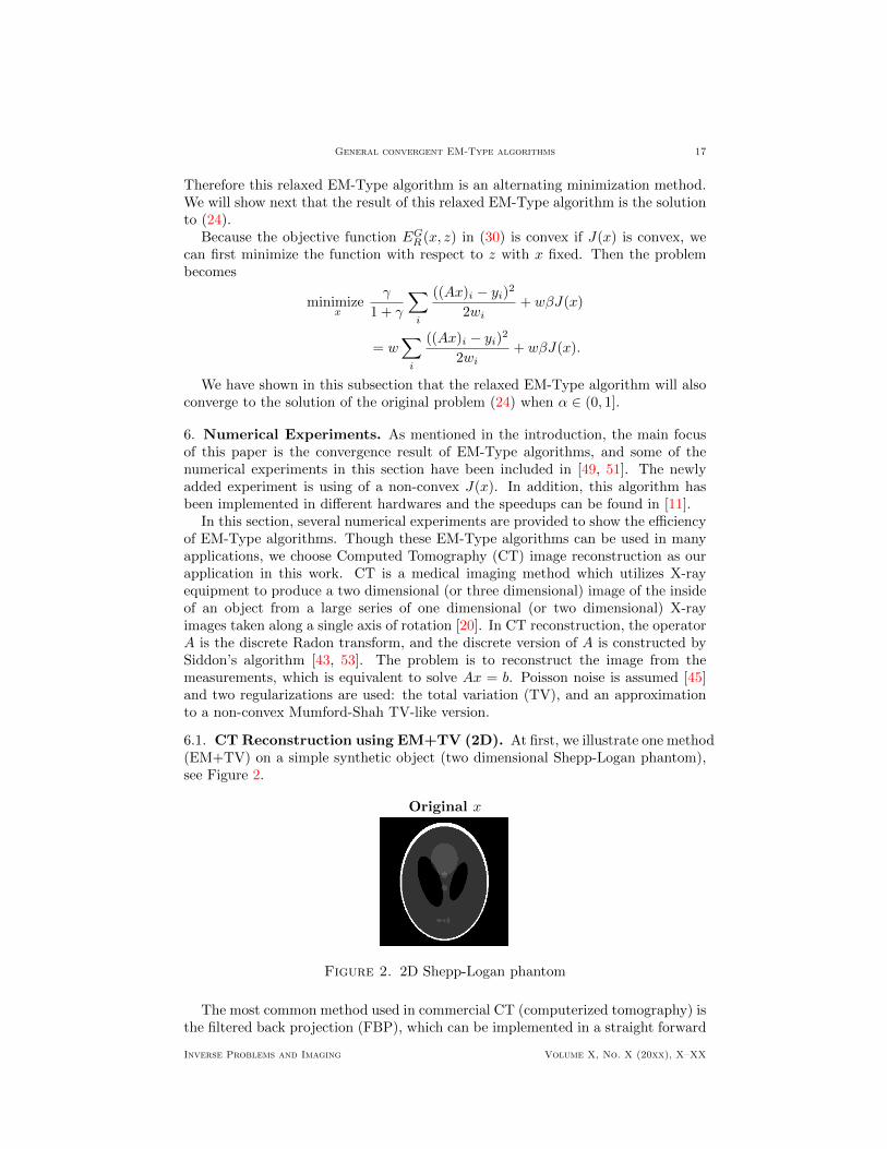
In the following experiment, we will compare the reconstruction results obtainedby EM+TV with those obtained by filtered back projection. Firstly we obtain themeasurements using Siddon’s algorithm. We consider both the noise-free and noisycases. For the FBP method, we present results using 36 views (every 10 degrees;for each view there are 301 measurements), 180 views, and 360 views. In order toshow that we can reduce the number of views by using EM+TV, we only use 36views for the proposed method. The results are shown in Figure 3. We notice themuch improved results obtained with EM+TV using only 36 views, by comparisonwith FBP using 36, 180 or even 360 views. To solve the regularization step, we usesemi-implicit scheme for some iterations [49].

Noise-free caseFBP 36 views FBP 180 views FBP 360 views EM+TV 36 views

RMSE = 50.8394 RMSE = 14.1995 RMSE = 12.6068 RMSE = 2.3789

Noisy caseFBP 36 views FBP 180 views FBP 360 views EM+TV 36 views

RMSE = 51.1003 RMSE = 14.3698 RMSE = 12.7039 RMSE = 3.0868

Figure 3. Top from left to right: reconstruction result in thenoise-free case using FBP with 36, 180 and 360 views, and resultusing EM+TV with 36 views. Bottom from left to right: recon-struction result in the noisy case using FBP with 36, 180 and 360views, and result using EM+TV with 36 views. The root meansquare errors are also given.

Inverse Problems and Imaging Volume X, No. X (20xx), X–XX

General convergent EM-Type algorithms 19

6.2. CT Reconstruction using EM+MSTV (2D). Instead of TV regulariza-tion, we will show the results using a modified TV-like regularization, which is calledMumford-Shah TV (MSTV) [40]. This regularization is

J(x, v) =

∫Ω

v2|∇x|+ α

∫Ω

(ε|∇v|2 +

(v − 1)2

4ε

),

which has two variables x and v, and Ω is the image domain. In the continuouscase, it is shown by Alicandro et al. [2] that J(x, v) will Γ-converge to∫

Ω\K|∇x|+ α

∫K

|x+ − x−|1 + |x+ − x−|

dH1 + |Dcx|(Ω),

where x+ and x− denote the image values on two sides of the edge set K, H1 isthe one-dimensional Hausdorff measure and Dcx is the Cantor part of the measure-valued derivative Dx.

The comparisons between EM+TV and EM+MSTV in both noise-free and noisycases are shown in Figure 4. From the results, we can see that with MSTV, thereconstructed images will be better than with TV only, visually and according tothe root-mean-squared-error (RMSE).

TV without noise MSTV without noise TV with noise MSTV with noise

RMSE = 2.33 RMSE = 1.58 RMSE = 3.33 RMSE = 2.27

−0.15

−0.1

−0.05

0

0.05

0.1

0.15

−0.1

−0.08

−0.06

−0.04

−0.02

0

0.02

0.04

0.06

0.08

0.1

−0.25

−0.2

−0.15

−0.1

−0.05

0

0.05

0.1

0.15

0.2

−0.15

−0.1

−0.05

0

0.05

0.1

0.15

Figure 4. Comparisons of TV regularization and MSTV regular-ization for both without and with noise cases. Top row: recon-structed images by these two methods in both cases. Bottom row:differences (errors) between the reconstructed images and originalphantom image. The RMSEs and differences show that MSTV canprovide better results than TV only.

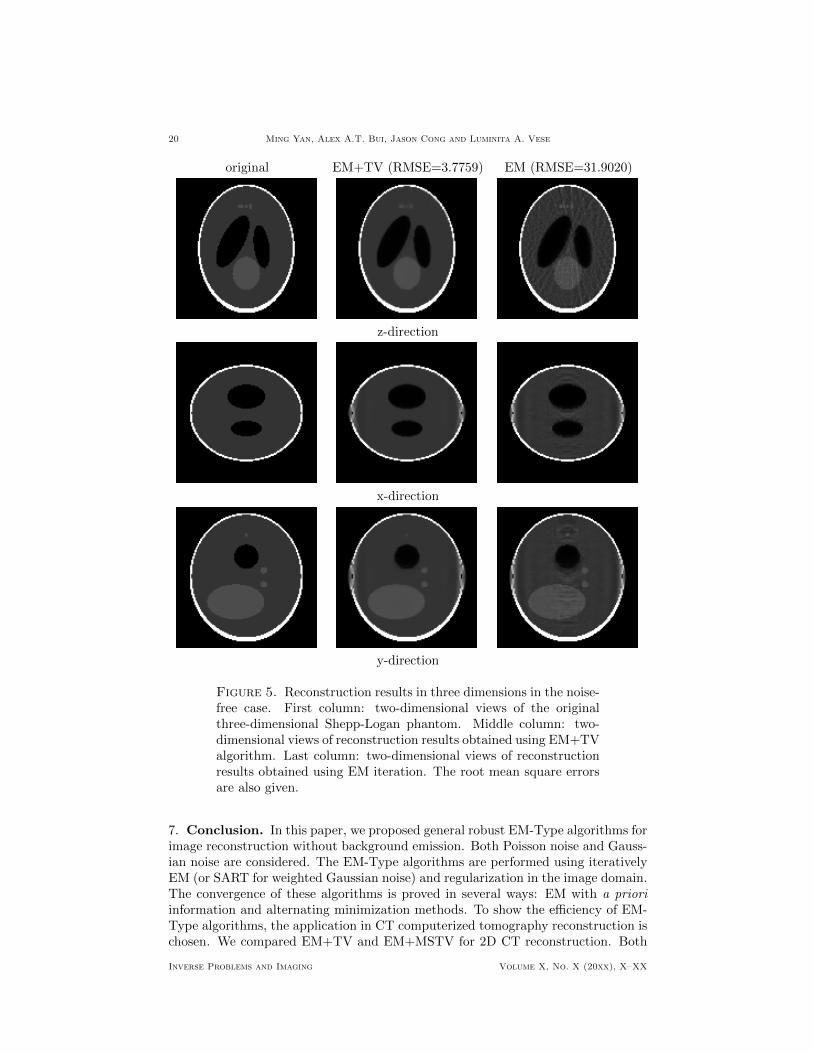
6.3. CT Reconstruction using EM+TV (3D). In this experiment, we willshow the reconstruction results using EM+TV for a three dimensional phantomimage. The image chosen is the 128 × 128 × 128 Shepp-Logan phantom, and thesinogram data is obtained from 36 views. The result is compared with the oneobtained using the EM step only in Figure 5.

Inverse Problems and Imaging Volume X, No. X (20xx), X–XX

20 Ming Yan, Alex A.T. Bui, Jason Cong and Luminita A. Vese

original EM+TV (RMSE=3.7759) EM (RMSE=31.9020)

z-direction

x-direction

y-direction

Figure 5. Reconstruction results in three dimensions in the noise-free case. First column: two-dimensional views of the originalthree-dimensional Shepp-Logan phantom. Middle column: two-dimensional views of reconstruction results obtained using EM+TValgorithm. Last column: two-dimensional views of reconstructionresults obtained using EM iteration. The root mean square errorsare also given.

7. Conclusion. In this paper, we proposed general robust EM-Type algorithms forimage reconstruction without background emission. Both Poisson noise and Gauss-ian noise are considered. The EM-Type algorithms are performed using iterativelyEM (or SART for weighted Gaussian noise) and regularization in the image domain.The convergence of these algorithms is proved in several ways: EM with a prioriinformation and alternating minimization methods. To show the efficiency of EM-Type algorithms, the application in CT computerized tomography reconstruction ischosen. We compared EM+TV and EM+MSTV for 2D CT reconstruction. Both

Inverse Problems and Imaging Volume X, No. X (20xx), X–XX

General convergent EM-Type algorithms 21

methods can give us good results by using undersampled data comparing to thefiltered back projection. Results from EM+MSTV have sharper edges than thosefrom EM+TV. Also EM+TV is used for 3D CT reconstruction and the performanceis better than using EM only (without regularization term) for undersampled data.

REFERENCES

[1] R. Acar and C. R. Vogel, Analysis of bounded variation penalty methods for ill-posed problems,Inverse Problems, 10 (1994), 1217–1229.

[2] R. Alicandro, A. braides and J. Shah, Free-discontinuity problems via functionals involving

the L1-norm of the gradient and their approximation, Interfaces and Free Boundaries, 1(1999), 17–37.

[3] A. Andersen, Algebraic reconstruction in CT from limited views, IEEE Transactions on Med-

ical Imaging, 8 (1989), 50–55.[4] A. Andersen and A. Kak, Simultaneous algebraic reconstruction technique (SART): a superior

implementation of the ART algorithm, Ultrasonic Imaging, 6 (1984), 81–94.

[5] C. Atkinson and J. Soria, An efficient simultaneous reconstruction technique for tomographicparticle image velocimetry, Experiments in Fluids, 47 (2009), 553–568.

[6] C. Brune, M. Burger, A. Sawatzky, T. Kosters and F. Wubbeling, Forward-Backward EM-TVmethods for inverse problems with Poisson noise, Preprint, august 2009.

[7] C. Brune, A. Sawatzky and M. Burger, Bregman-EM-TV methods with application to optical

nanoscopy, Lecture Notes in Computer Science, 5567 (2009), 235–246.[8] C. Brune, A. Sawatzky and M. Burger, Primal and dual Bregman methods with application

to optical nanoscopy, International Journal of Computer Vision, 92 (2011), 211–229.

[9] Y. Censor and T. Elfving, Block-iterative algorithms with diagonally scaled oblique projectionsfor the linear feasibility problem, SIAM Journal on Matrix Analysis and Applications, 24

(2002), 40–58.

[10] Y. Censor, D. Gordon and R. Gordon, Component averaging: An efficient iterative parallelalgorithm for large and sparse unstructured problems, Parallel Computing, 27 (2001), 777–

808.

[11] J. Chen, J. Cong, L. A. Vese, J. D. Villasenor, M. Yan and Y. Zou, A hybrid architecture forcompressive sensing 3-D CT reconstruction, IEEE Journal on Emerging and Selected Topics

in Circuits and Systems, 2 (2012), 616–625.

[12] J. A. Conchello and J. G. McNally, Fast regularization technique for expectation maximizationalgorithm for optical sectioning microscopy, in “Proceeding of SPIE Symposium on Electronic

Imaging Science and Technology”, 2655 (1996), 199–208.[13] A. Dempster, N. Laird and D. Rubin, Maximum likelihood from incomplete data via the EM

algorithm, Journal of the Royal Statistical Society Series B, 39 (1977), 1–38.

[14] N. Dey, L. Blanc-Feraud, C. Zimmer, P. Roux, Z. Kam, J. C. Olivo-Marin and J. Zerubia,Richardson-Lucy algorithm with total variation regularization for 3D confocal microscope

deconvolution, Microscopy Research and Technique, 69 (2006), 260–266.[15] S. Geman and D. Geman, Stochastic relaxation, Gibbs distributions, and the Bayesian

restoration of images, IEEE Transactions on Pattern Analysis and Machine Intelligence, 6

(1984), 721–741.

[16] R. Gordon, R. Bender and G. Herman, Algebraic reconstruction techniques (ART) for three-dimensional electron microscopy and X-ray photography, Journal of Theoretical Biology, 29

(1970), 471–481.[17] P. J. Green, On use of the EM algorithm for penalized likelihood estimation, Journal of the

Royal Statistical Society Series B, 52 (1990), 443–452.

[18] U. Grenander, Tutorial in pattern theory, Lecture Notes Volume, Division of Applied Math-ematics, Brown University, 1984.

[19] Z. T. Harmany, R. F. Marcia and R. M. Willett, Sparse Poisson intensity reconstruction

algorithms, in “Proceedings of IEEE/SP 15th Workshop on Statistical Signal Processing”,(2009), 634–637.

[20] G. Herman, “Fundamentals of Computerized Tomography: Image Reconstruction From Pro-

jection”, Springer, 2009.[21] H. Hurwitz, Entropy reduction in Bayesian analysis of measurements, Physics Review A, 12

(1975), 698–706.

Inverse Problems and Imaging Volume X, No. X (20xx), X–XX

22 Ming Yan, Alex A.T. Bui, Jason Cong and Luminita A. Vese

[22] S. Jafarpour, R. Willett, M. Raginsky and R. Calderbank, Performance bounds for expander-based compressed sensing in the presence of Poisson noise, in “Proceedings of the IEEE

Forty-Third Asilomar Conference on Signals, Systems and Computers”, (2009), 513–517.

[23] X. Jia, Y. Lou, R. Li, W. Y. Song and S. B. Jiang, GPU-based fast cone beam CT recon-struction from undersampled and noisy projection data via total variation, Medical Physics,

37 (2010), 1757–1760.[24] M. Jiang and G. Wang, Convergence of the simultaneous algebraic reconstruction technique

(SART), IEEE Transaction on Image Processing, 12 (2003), 957–961.

[25] M. Jiang and G. Wang, Convergence studies on iterative algorithms for image reconstruction,IEEE Transactions on Medical Imaging, 22 (2003), 569–579.

[26] S. Joshi and M. I. Miller, Maximum a posteriori estimation with Good’s roughness for three-

dimensional optical sectioning microscopy, Journal of the Optical Society of America A, 10(1993), 1078–1085.

[27] M. Jung, E. Resmerita and L. A. Vese, Dual norm based iterative methods for image restora-

tion, Journal of Mathematical Imaging and Vision, 44 (2012), 128–149.[28] A. Kak and M. Slaney, “Principles of Computerized Tomographic Imaging”, Society of In-

dustrial and Applied Mathematics, 2001.

[29] W. Karush, “Minima of Functions of Several Variables With Inequalities as Side Constraints”,Master’s thesis, Department of Mathematics, University of Chicago, Chicago, Illinois, 1939.

[30] H. Kuhn and A. Tucker, Nonlinear programming, in “Proceedings of the Second BerkeleySymposium on Mathematical Statistics and Probability”, (1951), 481–492.

[31] T. Le, R. Chartrand and T. J. Asaki, A variational approach to reconstructing images cor-

rupted by Poisson noise, Journal of Mathematical Imaging and Vision, 27 (2007), 257–263.[32] E. Levitan and G. T. Herman, A maximum a posteriori probability expectation maximization

algorithm for image reconstruction in emission tomography, IEEE Transactions on Medial

Imaging, 6 (1987), 185–192.[33] L. B. Lucy, An iterative technique for the rectification of observed distributions, Astronomical

Journal, 79 (1974), 745–754.

[34] J. Markham and J. A. Conchello, Fast maximum-likelihood image-restoration algorithms forthree-dimensional fluorescence microscopy, Journal of the Optical Society America A, 18

(2001), 1052–1071.

[35] F. Natterer and F. Wubbeling, “Mathematical Methods in Image Reconstruction”, Societyfor Industrial and Applied Mathematics, Philadelphia, PA, USA, 2001.

[36] Y. Pan, R. Whitaker, A. Cheryauka and D. Ferguson, Feasibility of GPU-assisted iterativeimage reconstruction for mobile C-arm CT , in “Proceedings of International Society for

Photonics and Optonics” SPIE 7258 (2009), 72585J.

[37] W. H. Richardson, Bayesian-based iterative method of image restoration, Journal of theOptical Society America, 62 (1972), 55–59.

[38] L. Rudin, S. Osher and E. Fatemi, Nonlinear total variation based noise removal algorithms,Physica D, 60 (1992), 259–268.

[39] S. Setzer, G. Steidl and T. Teuber, Deblurring poissonian images by split Bregman techniques,

Journal of Visual Communication and Image Representation, 21 (2010), 193–199.

[40] H. Shah, A common framework for curve evolution, segmentation and anisotropic diffusion,in “Proceeding of IEEE Conference on Computer Vision and Pattern Recognition”, (1996),

136–142.[41] L. Shepp and B. Logan, The Fourier reconstruction of a head section, IEEE Transaction on

Nuclear Science, 21 (1974), 21–34.

[42] L. Shepp and Y. Vardi, Maximum likelihood reconstruction for emission tomography, IEEE

Transaction on Medical Imaging, 1 (1982), 113–122.[43] R. Siddon, Fast calculation of the exact radiological path for a three-dimensional CT array,

Medical Physics, 12 (1986), 252–255.[44] E. Y. Sidky, R. Chartrand and X. Pan, Image reconstruction from few views by non-convex

optimization, in “IEEE Nuclear Science Symposium Conference Record”, 5 (2007).

[45] E. Y Sidky, J. H. Jorgensen and X. Pan, Convex optimization problem prototyping for im-age reconstruction in computed tomography with the Chambolle-Pock algorithm, Physics in

Medicine and Biology, 57 (2012), 3065.

[46] A. N. Tychonoff and V. Y. Arsenin, “Solution of Ill-posed Problems”, Winston & Sons,Washington, 1977.

Inverse Problems and Imaging Volume X, No. X (20xx), X–XX

General convergent EM-Type algorithms 23

[47] J. Wang and Y. Zheng, On the convergence of generalized simultaneous iterative reconstruc-tion algorithms, IEEE Transaction on Image Processing, 16 (2007), 1–6.

[48] R. M. Willett, Z. T. Harmany and R. F. Marcia, Poisson image reconstruction with total

variation regularization, Proceedings of 17th IEEE International Conference on Image Pro-cessing, (2010), 4177–4180.

[49] M. Yan and L. A. Vese, Expectation maximization and total variation based model for com-puted tomography reconstruction from undersampled data, in Proceeding of SPIE Medical

Imaging: Physics of Medical Imaging, 7961 (2011), 79612X.

[50] M. Yan, Convergence analysis of SART: optimization and statistics, International Journal ofComputer Mathematics, 90 (2013), 30–47.

[51] M. Yan, J. Chen, L. A. Vese, J. D. Villasenor, A. A. T. Bui and J. Cong, EM+TV based

reconstruction for cone-beam CT with reduced radiation, in “Lecture Notes in ComputerScience” 6938 (2011), 1–10.

[52] H. Yu and G. Wang, SART-type image reconstruction from a limited number of projections

with the sparsity constraint , Journal of Biomedical Imaging, 2010 (2010), 1–9.[53] H. Zhao and A. J. Reader, Fast ray-tracing technique to calculate line integral paths in voxel

arrays, in IEEE Nuclear Science Symposium Conference Record, 4 (2003), M11–197.

[54] D. Zhu, M. Razaz and R. Lee, Adaptive penalty likelihood for reconstruction of multi-dimensional confocal microscopy images, Computerized Medical Imaging and Graphics, 29

(2005), 319–331.[55] Compressive Sensing Resources, http://dsp.rice.edu/cs,

Received xxxx 20xx; revised xxxx 20xx.

Inverse Problems and Imaging Volume X, No. X (20xx), X–XX