expectation maximization algorithm
DESCRIPTION
Expectation Maximization Algorithm. Rong Jin. A Mixture Model Problem. Apparently, the dataset consists of two modes How can we automatically identify the two modes?. Gaussian Mixture Model (GMM). Assume that the dataset is generated by two mixed Gaussian distributions Gaussian model 1: - PowerPoint PPT PresentationTRANSCRIPT

Expectation Maximization Algorithm
Rong Jin
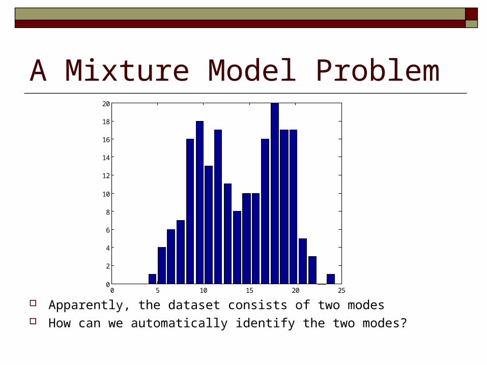
A Mixture Model Problem
Apparently, the dataset consists of two modes How can we automatically identify the two modes?
0 5 10 15 20 250
2
4
6
8
10
12
14
16
18
20

Gaussian Mixture Model (GMM) Assume that the dataset is generated by two
mixed Gaussian distributions Gaussian model 1: Gaussian model 2:
If we know the memberships for each bin, estimating the two Gaussian models is easy.
How to estimate the two Gaussian models without knowing the memberships of bins?
1 1 1 1, ; p
2 2 2 2, ; p

EM Algorithm for GMM Let memberships to be hidden variables
EM algorithm for Gaussian mixture model Unknown memberships:
Unknown Gaussian models:
Learn these two sets of parameters iteratively
1 21 2 1 2{ , ,..., } , , , ,..., ,n n nmx x x x x xm m
1 21 2, , , ,..., ,n nx x xm m m
1 1 1 1
2 2 2 2
, ;
, ;
p
p

Start with A Random Guess
Random assign the memberships to each bin
0 5 10 15 20 250
2
4
6
8
10
12
14
16
18
20
0 5 10 15 20 250
0.1
0.2
0.3
0.4
0.5
0.6
0.7
0.8
0.9
1

Start with A Random Guess
Random assign the memberships to each bin
Estimate the means and variance of each Gaussian model
0 5 10 15 20 250
0.1
0.2
0.3
0.4
0.5
0.6
0.7
0.8
0.9
10 5 10 15 20 25
0
2
4
6
8
10
12
14
16
18
20
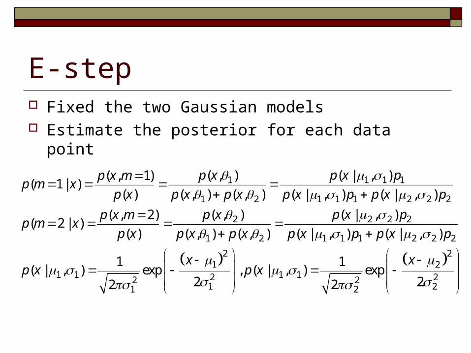
E-step Fixed the two Gaussian models Estimate the posterior for each data point
1 1 1 1
1 2 1 1 1 2 2 2
2 2 2 2
1 2 1 1 1 2 2 2
21
1 1 2211
( , ) ( | , )( , 1)( 1 | )
( ) ( , ) ( , ) ( | , ) ( | , )
( , ) ( | , )( , 2)( 2 | )
( ) ( , ) ( , ) ( | , ) ( | , )
1( | , ) exp
22
p x p x pp x mp m x
p x p x p x p x p p x p
p x p x pp x mp m x
p x p x p x p x p p x p
xp x
221 1 22
22
1, ( | , ) exp
22
xp x
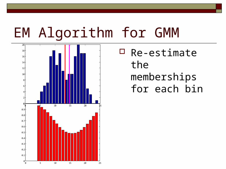
EM Algorithm for GMM Re-estimate the
memberships for each bin
0 5 10 15 20 250
0.1
0.2
0.3
0.4
0.5
0.6
0.7
0.8
0.9
10 5 10 15 20 25
0
2
4
6
8
10
12
14
16
18
20

1 21
1 1 1 2 2 21
ˆ ˆ( 1 | ) log ( , ) ( 2 | ) log ( , )
ˆ ˆ( 1 | ) log log ( | , ) ( 2 | ) log log ( | , )
n
i i i i i ii
n
i i i i i ii
l p m x p x p m x p x
p m x p p x p m x p p x
22 21 1 1
1 1 1 1
1 1
221 1 1
2 2 2
1 1
ˆ ˆ ˆ( 1 | ) ( 1 | ) ( 1 | ), ,
ˆ ˆ( 1 | ) ( 1 | )
ˆ ˆ ˆ( 2 | ) ( 2 | ) ( 2 | ), ,
ˆ ˆ( 2 | ) ( 2 | )
n n ni i i i i i i ii i i
n ni i i ii i
n n ni i i i i i i ii i i
n ni i i ii i
p m x p m x x p m x xp
n p m x p m x
p m x p m x x p m x xp
n p m x p m x
22
M-Step Fixed the memberships Re-estimate the two model Gaussian
Weighted by posteriors
Weighted by posteriors

EM Algorithm for GMM Re-estimate the
memberships for each bin
Re-estimate the models
0 5 10 15 20 250
0.1
0.2
0.3
0.4
0.5
0.6
0.7
0.8
0.9
1 0 5 10 15 20 250
2
4
6
8
10
12
14
16
18
20

At the 5-th Iteration Red Gaussian
component slowly shifts toward the left end of the x axis
0 5 10 15 20 250
2
4
6
8
10
12
14
16
18
20
0 5 10 15 20 250
0.1
0.2
0.3
0.4
0.5
0.6
0.7
0.8
0.9

At the10-th Iteration
Red Gaussian component still slowly shifts toward the left end of the x axis
0 5 10 15 20 250
2
4
6
8
10
12
14
16
18
20
0 5 10 15 20 250
0.1
0.2
0.3
0.4
0.5
0.6
0.7
0.8
0.9

At the 20-th Iteration Red Gaussian
component make more noticeable shift toward the left end of the x axis
0 5 10 15 20 250
2
4
6
8
10
12
14
16
18
20
0 5 10 15 20 250
0.1
0.2
0.3
0.4
0.5
0.6
0.7
0.8
0.9
1

At the 50-th Iteration Red Gaussian
component is close to the desirable location
0 5 10 15 20 250
2
4
6
8
10
12
14
16
18
20
0 5 10 15 20 250
0.1
0.2
0.3
0.4
0.5
0.6
0.7
0.8
0.9
1

At the 100-th Iteration The results are
almost identical to the ones for the 50-th iteration
0 5 10 15 20 250
2
4
6
8
10
12
14
16
18
20
0 5 10 15 20 250
0.1
0.2
0.3
0.4
0.5
0.6
0.7
0.8
0.9
1
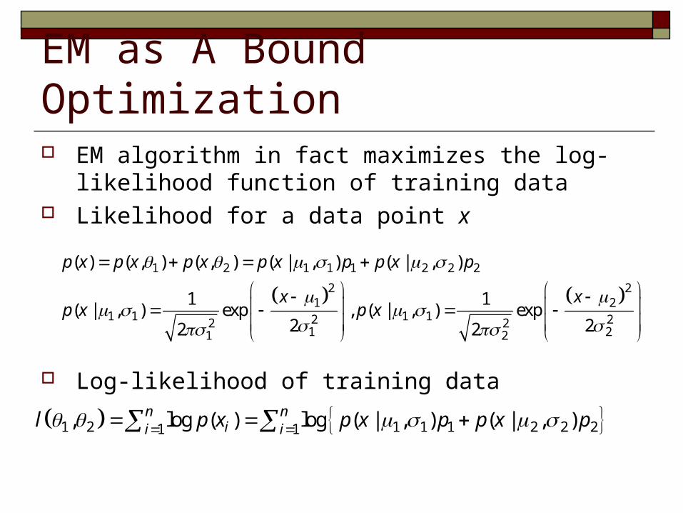
EM as A Bound Optimization EM algorithm in fact maximizes the log-likelihood function
of training data Likelihood for a data point x
Log-likelihood of training data
1 2 1 1 1 2 2 2
2 21 2
1 1 1 12 22 21 21 2
( ) ( , ) ( , ) ( | , ) ( | , )
1 1( | , ) exp , ( | , ) exp
2 22 2
p x p x p x p x p p x p
x xp x p x
1 1 1 2 2 21 1log ( ) log ( | , ) ( | , )n nii il p x p x p p x p
EM as A Bound Optimization EM algorithm in fact maximizes the log-likelihood function
of training data Likelihood for a data point x
Log-likelihood of training data
1 2 1 1 1 2 2 2
2 21 2
1 1 1 12 22 21 21 2
( ) ( , ) ( , ) ( | , ) ( | , )
1 1( | , ) exp , ( | , ) exp
2 22 2
p x p x p x p x p p x p
x xp x p x
1 2 1 1 1 2 2 21 1, log ( ) log ( | , ) ( | , )n nii il p x p x p p x p
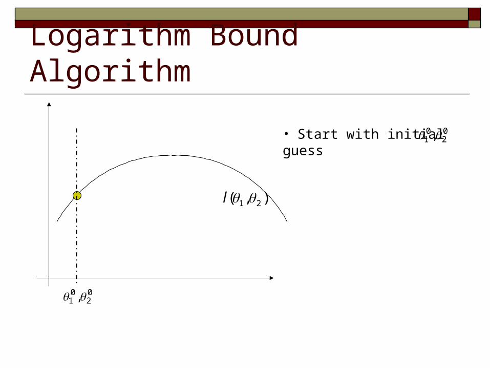
Logarithm Bound Algorithm
1 2( , )l
• Start with initial guess
0 01 2,
0 01 2,

Logarithm Bound Algorithm
• Start with initial guess
0 01 2 1 2 1 2( , ) ( , ) ( , )l l Q
• Come up with a lower bounded
0 01 2,
1 2 0,
1 2( , )l 0 0
1 2 1 2 1 2( , ) ( , ) ( , )l l Q
1 2
0 01 1 2 2
( , ) is a concave function
Touch point: ( , ) 0
Q
Q
Touch Point

Logarithm Bound Algorithm
• Start with initial guess
0 01 2 1 2 1 2( , ) ( , ) ( , )l l Q
• Come up with a lower bounded
0 01 2,
1 2 0,
1 2( , )l 0 0
1 2 1 2 1 2( , ) ( , ) ( , )l l Q
1 2
0 01 1 2 2
( , ) is a concave function
Touch point: ( , ) 0
Q
Q
• Search the optimal solution that maximizes 1 2( , )Q
1 11 2,

Logarithm Bound Algorithm
• Start with initial guess
1 11 2 1 2 1 2( , ) ( , ) ( , )l l Q
• Come up with a lower bounded
0 01 2,
1 2 0,
1 2( , )l 0 0
1 2 1 2 1 2( , ) ( , ) ( , )l l Q
1 2
0 01 1 2 2
( , ) is a concave function
Touch point: ( , ) 0
Q
Q
• Search the optimal solution that maximizes
• Repeat the procedure
1 2( , )Q 1 1
1 2, 2 21 2,
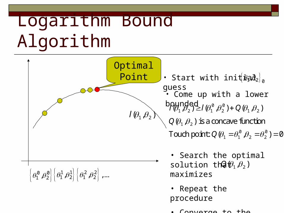
Logarithm Bound AlgorithmOptimal
Point
1 2( , )l
0 01 2, 1 1
1 2, 2 21 2, ,...
• Start with initial guess
• Come up with a lower bounded
1 2 0,
0 01 2 1 2 1 2( , ) ( , ) ( , )l l Q
1 2
0 01 1 2 2
( , ) is a concave function
Touch point: ( , ) 0
Q
Q
• Search the optimal solution that maximizes
• Repeat the procedure
• Converge to the local optimal
1 2( , )Q

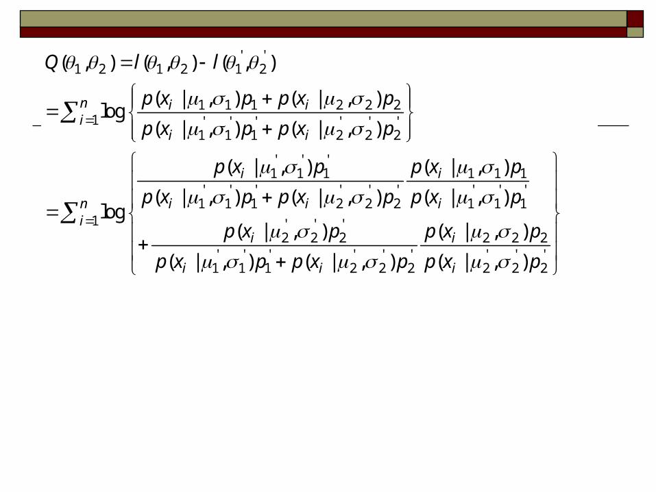
EM as A Bound Optimization Parameter for previous iteration: Parameter for current iteration: Compute
' '1 2,
1 2,
1 2( , )Q

' '1 2 1 2 1 2
1 1 1 2 2 21 ' ' ' ' ' '
1 1 1 2 2 2
' ' '1 1 1 1 1 1
' ' ' ' ' ' ' ' '1 1 1 2 2 2 1 1 1
'2
( , ) ( , ) ( , )
( | , ) ( | , )log
( | , ) ( | , )
( | , ) ( | , )
( | , ) ( | , ) ( | , )log
( | ,
n i ii
i i
i i
i i i
i
Q l l
p x p p x p
p x p p x p
p x p p x p
p x p p x p p x p
p x
1 ' '2 2 2 2 2
' ' ' ' ' ' ' ' '1 1 1 2 2 2 2 2 2
' ' '1 1 1 1 1 1
' ' ' ' ' ' ' ' '1 1 1 2 2 2 1 1 1
' ' '2 2 2
' '1 1
) ( | , )
( | , ) ( | , ) ( | , )
( | , ) ( | , )log
( | , ) ( | , ) ( | , )
( | , )
( | , )
ni
i
i i i
i i
i i i
i
i
p p x p
p x p p x p p x p
p x p p x p
p x p p x p p x p
p x p
p x p
12 2 2
' ' ' ' ' ' '1 2 2 2 2 2 2
' '1 1 1 2 2 21 21 ' ' ' ' ' '
1 1 1 2 2 2
( | , )log
( | , ) ( | , )
( | , ) ( | , )( | ) log ( | ) log
( | , ) ( | , )
ni
i
i i
n i ii ii
i i
p x p
p x p p x p
p x p p x pp x p x
p x p p x p
Concave property of logarithm function
log( (1 ) ) log (1 ) log
0 1, , 0
p p p p
p

' '1 2 1 2 1 2
1 1 1 2 2 21 ' ' ' ' ' '
1 1 1 2 2 2
' ' '1 1 1 1 1 1
' ' ' ' ' ' ' ' '1 1 1 2 2 2 1 1 1
'2
( , ) ( , ) ( , )
( | , ) ( | , )log
( | , ) ( | , )
( | , ) ( | , )
( | , ) ( | , ) ( | , )log
( | ,
n i ii
i i
i i
i i i
i
Q l l
p x p p x p
p x p p x p
p x p p x p
p x p p x p p x p
p x
1 ' '2 2 2 2 2
' ' ' ' ' ' ' ' '1 1 1 2 2 2 2 2 2
' ' '1 1 1 1 1 1
' ' ' ' ' ' ' ' '1 1 1 2 2 2 1 1 1
' ' '2 2 2
' '1 1
) ( | , )
( | , ) ( | , ) ( | , )
( | , ) ( | , )log
( | , ) ( | , ) ( | , )
( | , )
( | , )
ni
i
i i i
i i
i i i
i
i
p p x p
p x p p x p p x p
p x p p x p
p x p p x p p x p
p x p
p x p
12 2 2
' ' ' ' ' ' '1 2 2 2 2 2 2
' ' ' '1 1 1 2 2 21 1 2 1 1 21 ' ' ' ' ' '
1 1 1 2 2 2
( | , )log
( | , ) ( | , )
( | , ) ( | , )( 1 | ; , ) log ( 2 | ; , ) log
( | , ) ( | , )
ni
i
i i
n i ii ii
i i
p x p
p x p p x p
p x p p x pp m x p m x
p x p p x p
Definition of posterior' ' '
' '1 1 11 1 2' ' ' ' ' '
1 1 1 2 2 2
( | , )( 1 | ; , )
( | , ) ( | , )i
ii i
p x pp m x
p x p p x p
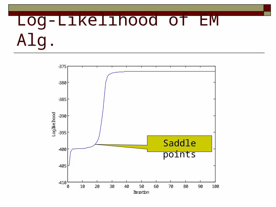
Log-Likelihood of EM Alg.
0 10 20 30 40 50 60 70 80 90 100-410
-405
-400
-395
-390
-385
-380
-375
Iteration
Logl
ikel
hood
Saddle points

Maximize GMM Model
What is the global optimal solution to GMM?
Maximizing the objective function of GMM is ill-posed problem
1 1 1 2 2 21 1log ( ) log ( | , ) ( | , )n nii il p x p x p p x p
2 21 2
1 1 1 12 22 21 21 2
1 1( | , ) exp , ( | , ) exp
2 22 2
x xp x p x
11 1 1 1 2 1 2, 0, , 1, 0.5
nii x
x p pn

Identify Hidden Variables For certain learning problems, identifying hidden variables is
not a easy task Consider a simple translation model
For a pair of English and Chinese sentences:
A simple translation model is
The log-likelihood of training corpus
1 2 1 2: ( , ,..., ) : ( , ,..., )s le e e e c c c c
11 1Pr( | ) Pr( | ) Pr( | )s s tj j kkj je c e c e c
1 1, ,..., ,n ne c e c
, ,1 1 1 1log Pr( | ) log Pr( | )i in n e ci i i j i ki i j kl e c e c
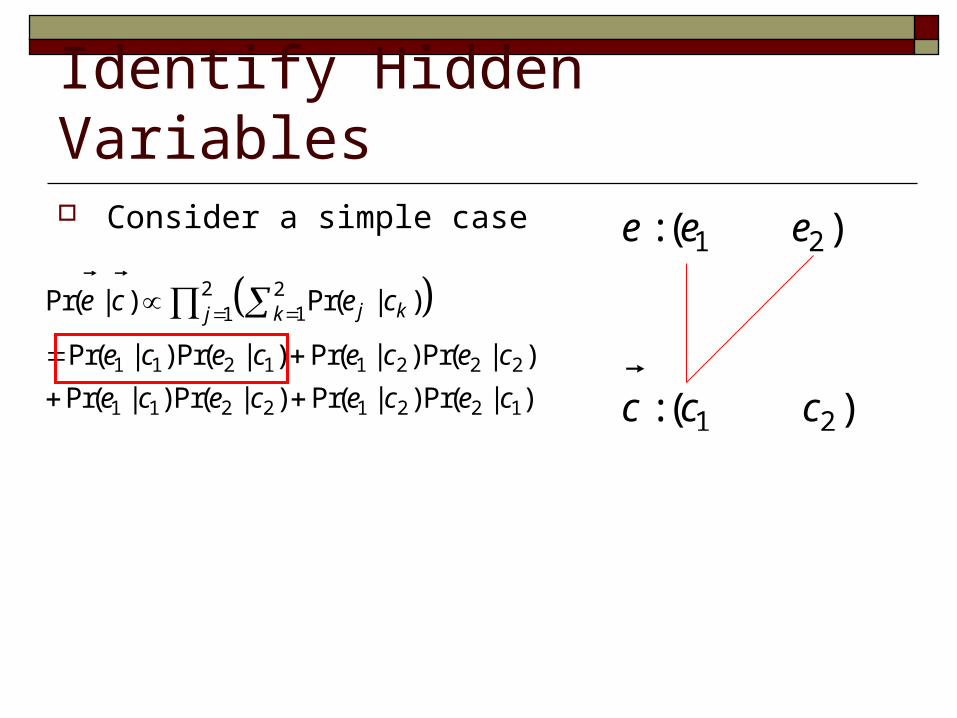
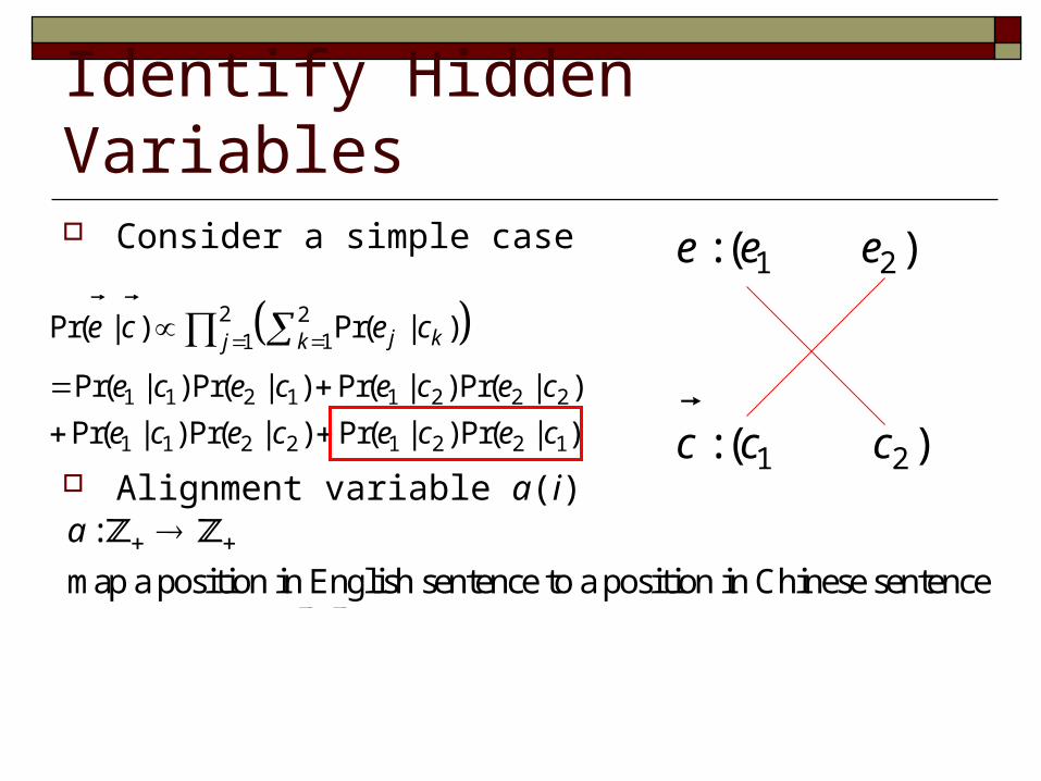
Identify Hidden Variables Consider a simple case
Alignment variable a(i)
Rewrite
1 2
1 2
: ( )
: ( )
e e e
c c c
2 211
1 1 2 1 1 2 2 2
1 1 2 2 1 2 2 1
Pr( | ) Pr( | )
Pr( | ) Pr( | ) Pr( | ) Pr( | )
Pr( | ) Pr( | ) Pr( | ) Pr( | )
j kkje c e c
e c e c e c e c
e c e c e c e c
:
map a position in English sentence to a position in Chinese sentence
a
1 (1) 2 (2)Pr( | ) Pr( | ) Pr( | )a aae c e c e c

EM Algorithm for A Translation Model Introduce an alignment variable for each translation pair
EM algorithm for the translation model E-step: compute the posterior for each alignment variable M-step: estimate the translation probability Pr(e|c)
1 1 2 21 2, , , , , ,..., , , ,n n na a ae c e c e c
Pr( | , )j j ja e c
| | | |
, , ( ) , , ( )1 1| | | |
', , '( ) , ,' 1
1 1
Pr( | ) Pr( | )Pr( , , )
Pr( | , )Pr( ', , )
Pr( | ) Pr( | )
j j
j ji
e e
j k j a k j k j a kj j k k
j j e ej j ca
j k j a k j s j ta tk k
e c e ca e c
a e ca e c
e c e c
We are luck here. In general, this step can be extremely difficult and usually requires approximate approaches
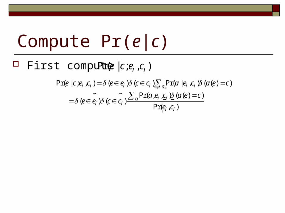
Compute Pr(e|c) First compute
,
| |
, ,11^
| |
, ,11
Pr( | ; , ) ( ) ( ) Pr( | , ) ( ( ) )
Pr( , , ) ( ( ) )( ) ( )
Pr( , )
Pr( | ) Pr( | )
( ) ( )
Pr( | )
(
ji
j k
ji
i i i i i ia
i iai i
i i
ec
j s j ttk e e
i i ec
j s j ttk
e c e c e e c c a e c a e c
a e c a e ce e c c
e c
e c e c
e e c c
e c
,1
Pr( | )) ( )
Pr( | )ii i c
j tt
e ce e c c
e c
Pr( | ; , )i ie c e c
1Pr( | ) Pr( | ; , )ni iie c e c e c

, ,1 1 1 1
, ,1 1 1 1
Pr( | ) for the current iteration
' Pr'( | ) for the previous iteration
( ) log Pr( | ; ) log Pr( | )
( ') log Pr( | ; ') log Pr'( | )
i i
i i
n n e ci i i j i ki i j k
n n e ci i i j i ki i j k
e c
e c
l e c e c
l e c e c
θ
θ
θ θ
θ θ
, ,11 1
, ,1
Pr( | )( , ') ( ) ( ') log
Pr'( | )
i
i
i
ci j i kn e k
i j ci j i ll
e cQ l l
e c
θ θ θ θ
Bound Optimization for A Translation Model

Bound Optimization for A Translation Model
, ,11 1
, ,1
, , , ,1 1
1 , ,, ,1
, ,
,
Pr( | )( , ') ( ) ( ') log
Pr'( | )
Pr'( | ) Pr( | )log
Pr'( | )Pr'( | )
Pr'( | )
Pr'( |
i
i
i
ii
i
ci j i kn e k
i j ci j i ll
ci j i k i j i kn e
i j ck i j i ki j i ll
i j i k
i j
e cQ l l
e c
e c e c
e ce c
e c
e
θ θ θ θ
, ,1 1 1
, ,,1
Pr( | )log
Pr'( | ))i i
i
i j i kn e ci j k c
i j i ki ll
e c
e cc
1,1
Pr'( | )Pr( | ) ( ) ( )
Pr'( | )i
ni ii c
j tt
e ce c e e c c
e c

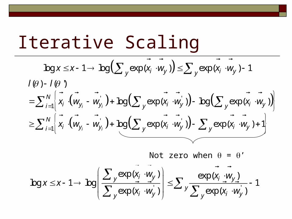
Iterative Scaling Maximum entropy model
1
exp( )exp( )( | ; ) , ( ) log
exp( ) exp( )iN i yy
train iy i yy y
x wx wp y x l D
x w x w
Iterative scaling All features Sum of features are constant
, 0i jx
,1d
i jj x g

Iterative Scaling Compute the empirical mean for each feature of every class,
i.e., for every j and every class y
Start w1 ,w2 …, wc = 0 Repeat
Compute p(y|x) for each training data point (xi, yi) using w from the previous iteration
Compute the mean of each feature of every class using the estimated probabilities, i.e., for every j and every y
Compute for every j and every y
Update w as
, ,1( , )
Ny j i j ii
e x y y N
, ,1( | )
Ny j i j ii
m x p y x N
, , ,j y j y j yw w w
, , ,1
log logj y j y j yw e mg
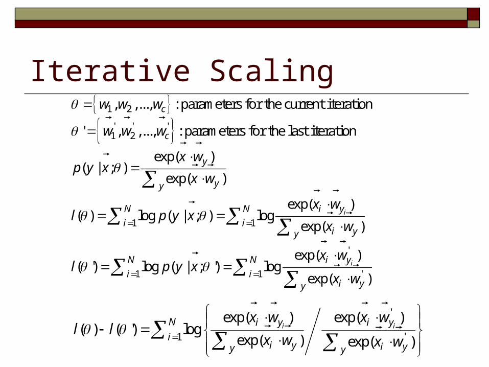
Iterative Scaling
1 2
' ' '1 2
1
, ,..., : parameters for the current iteration
' , ,..., : parameters for the last iteration
exp( )( | ; )
exp( )
exp( )( ) log ( | ; ) log
exp( )i
c
c
y
yy
N i y
i ii yy
w w w
w w w
x wp y x
x w
x wl p y x
x w
1
'
'1 1
exp( )( ') log ( | ; ') log
exp( )i
N
N N i y
i ii yy
x wl p y x
x w
'
'1
exp( ) exp( )( ) ( ') log
exp( ) exp( )i iN i y i y
ii y i yy y
x w x wl l
x w x w

Iterative Scaling
'
'1
' '1
exp( ) exp( )( ) ( ') log
exp( ) exp( )
log exp( ) log exp( )
i i
i i
N i y i y
ii y i yy y
Ni y y i y i yi y y
x w x wl l
x w x w
x w w x w x w
Can we use the concave property of logarithm function?
No, we can’t because we need a lower bound

Iterative Scaling
log 1 log exp( ) exp( ) 1i y i yy yx x x w x w
' '1
' '1
( ) ( ')
log exp( ) log exp( )
log exp( ) exp( ) 1
i i
i i
Ni y y i y i yi y y
Ni y y i y i yi y y
l l
x w w x w x w
x w w x w x w
• Weights still couple with each other
• Still need further decomposition
yw
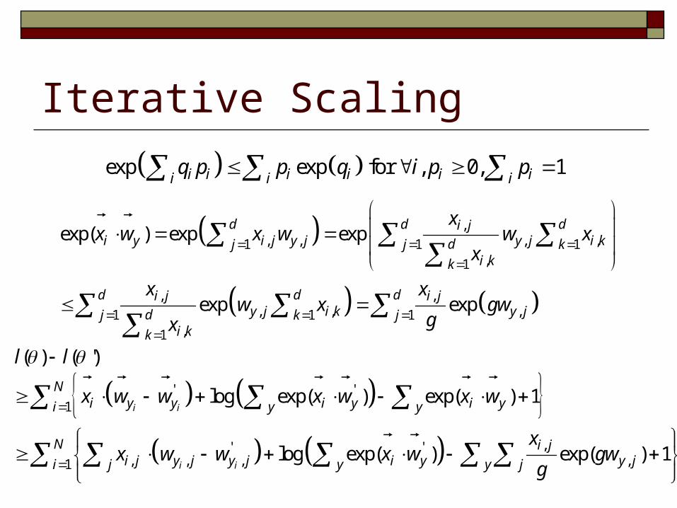
Iterative Scaling
,, , , ,1 1 1
,1
, ,, , ,1 1 1
,1
exp( ) exp exp
exp exp
d d di ji y i j y j y j i kdj j k
i kk
d d di j i jy j i k y jdj k j
i kk
xx w x w w x
x
x xw x gw
gx
' '1
,' ', , , ,1
( ) ( ')
log exp( ) exp( ) 1
log exp( ) exp( ) 1
i i
i i
Ni y y i y i yi y y
N i ji j y j y j i y y ji j y y j
l l
x w w x w x w
xx w w x w gw
g
exp exp for , 0, 1i i i i i ii i iq p p q i p p
Iterative Scaling
,' ', , , ,1
,' ', , , ,1 1
( , ') log exp( ) exp( ) 1
log exp( ) 1 , exp( )
i i
N i ji j y j y j i y y ji j y y j
N N i ji y i j y j y j i y ji y i y j
xQ x w w x w gw
g
xx w x w w y y gw
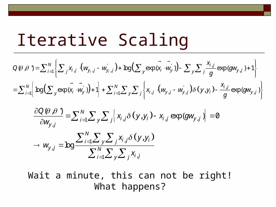
g
, , ,1,
,1,
,1
( , '), exp( ) 0
,log
Ni j i i j y ji y j
y j
Ni j ii y j
y j Ni ji y j
Qx y y x gw
w
x y yw
x
Wait a minute, this can not be right! What happens?
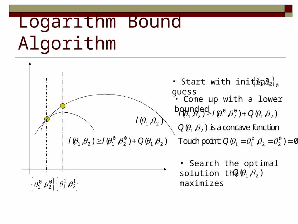
Logarithm Bound Algorithm
• Start with initial guess
0 01 2 1 2 1 2( , ) ( , ) ( , )l l Q
• Come up with a lower bounded
0 01 2,
1 2 0,
1 2( , )l 0 0
1 2 1 2 1 2( , ) ( , ) ( , )l l Q
1 2
0 01 1 2 2
( , ) is a concave function
Touch point: ( , ) 0
Q
Q
• Search the optimal solution that maximizes 1 2( , )Q
1 11 2,

Iterative Scaling
,' ', , , ,1 1
( , ')
log exp( ) 1 , exp( )N N i j
i y i j y j y j i y ji y i y j
Q
xx w x w w y y gw
g
,' ' ' ', , , ,1 1
,' ',1 1
( ', ')
log exp( ) 1 , exp( )
log exp( ) 1 exp( )
0
N N i ji y i j y j y j i y ji y i y j
N N i ji y y ji y i y j
Q
xx w x w w y y gw
g
xx w gw
g
Where does it go wrong?
Iterative Scaling
log 1 log exp( ) exp( ) 1i y i yy yx x x w x w
' '1
' '1
( ) ( ')
log exp( ) log exp( )
log exp( ) exp( ) 1
i i
i i
Ni y y i y i yi y y
Ni y y i y i yi y y
l l
x w w x w x w
x w w x w x w
Not zero when = ’
' '
exp( ) exp( )log 1 log 1
exp( ) exp( )
i yy i y
yi y i yy y
x w x wx x
x w x w
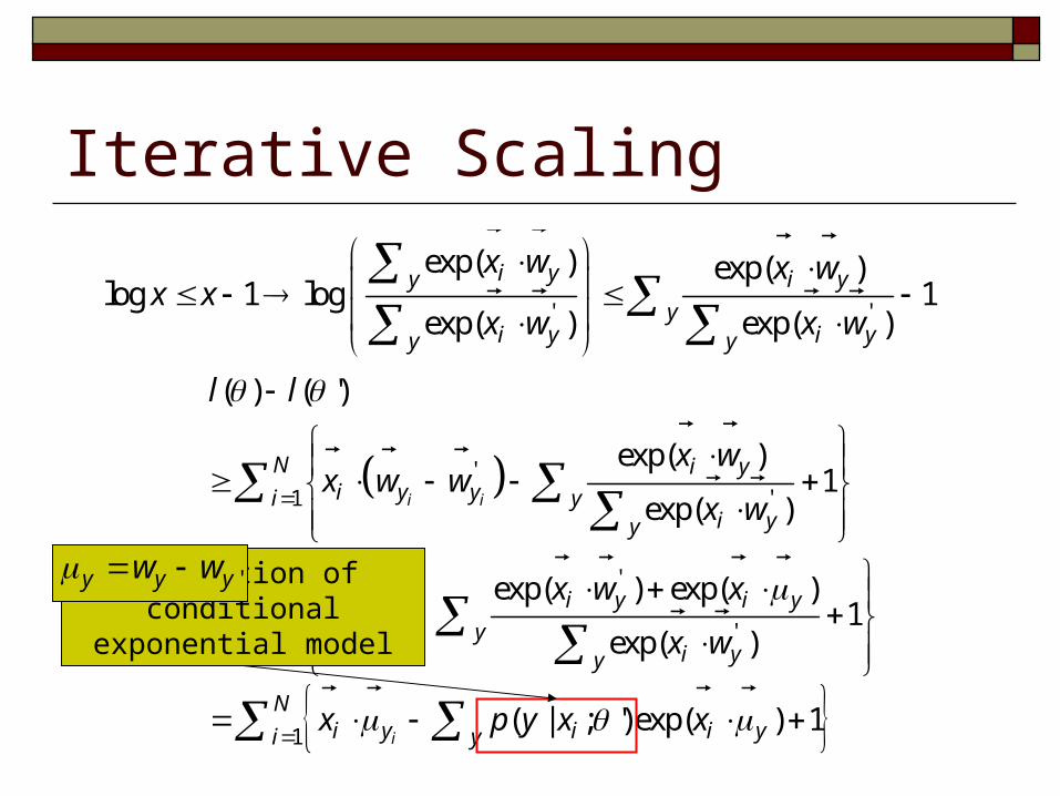
Iterative Scaling
''1
'
'1
1
( ) ( ')
exp( )1
exp( )
exp( ) exp( )1
exp( )
( | ; ') exp( ) 1
i i
i
i
N i yi y yi y
i yy
N i y i yi yi y
i yy
Ni y i i yi y
l l
x wx w w
x w
x w xx
x w
x p y x x
' '
exp( ) exp( )log 1 log 1
exp( ) exp( )
i yy i y
yi y i yy y
x w x wx x
x w x w
Definition of conditional exponential model
'y y yw w

Iterative Scaling
,, , , ,1 1 1
,1
, ,, , ,1 1 1
,1
exp( ) exp exp
exp exp
d d di ji y i j y j y j i kdj j k
i kk
d d di j i jy j i k y jdj k j
i kk
xx x x
x
x xx g
gx
1
,, , ,1
,, , ,1
( ) ( ') ( | ; ') exp( ) 1
( | ; ') exp( ) 1
( , ) ( | ; ') exp( ) 1
i
i
Ni y i i yi y
N i ji j y j i y ji j y j
N i ji j y j i i y ji j y
l l x p y x x
xx p y x g
g
xx y y p y x g
g
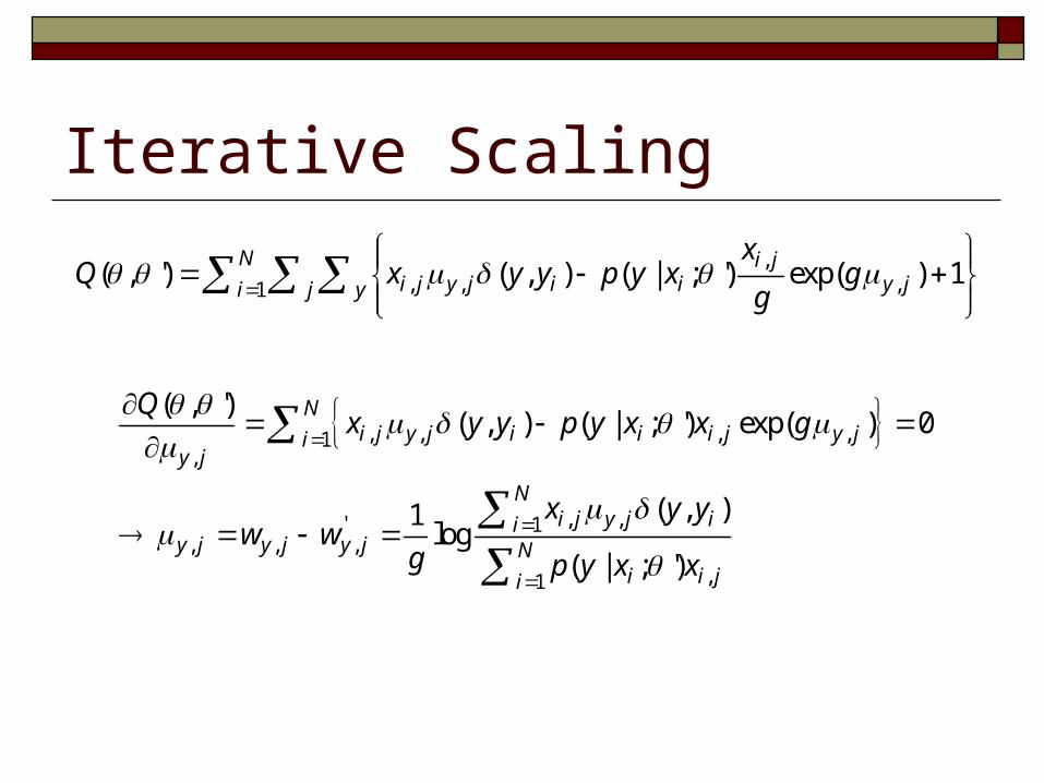
Iterative Scaling
,, , ,1
( , ') ( , ) ( | ; ') exp( ) 1N i j
i j y j i i y ji j y
xQ x y y p y x g
g
, , , ,1,
, ,' 1, , ,
,1
( , ')( , ) ( | ; ') exp( ) 0
( , )1log
( | ; ')
Ni j y j i i i j y ji
y j
Ni j y j ii
y j y j y j Ni i ji
Qx y y p y x x g
x y yw w
g p y x x
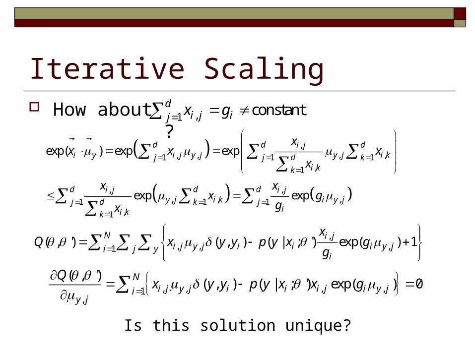
Iterative Scaling How about ? ,1 constantd
i j ij x g
,, , , ,1 1 1
,1
, ,, , ,1 1 1
,1
exp( ) exp exp
exp exp
d d di ji y i j y j y j i kdj j k
i kk
d d di j i jy j i k i y jdj k j
ii kk
xx x x
x
x xx g
gx
,, , ,1
( , ') ( , ) ( | ; ') exp( ) 1N i j
i j y j i i i y ji j yi
xQ x y y p y x g
g
, , , ,1,
( , ')( , ) ( | ; ') exp( ) 0
Ni j y j i i i j i y ji
y j
Qx y y p y x x g
Is this solution unique?
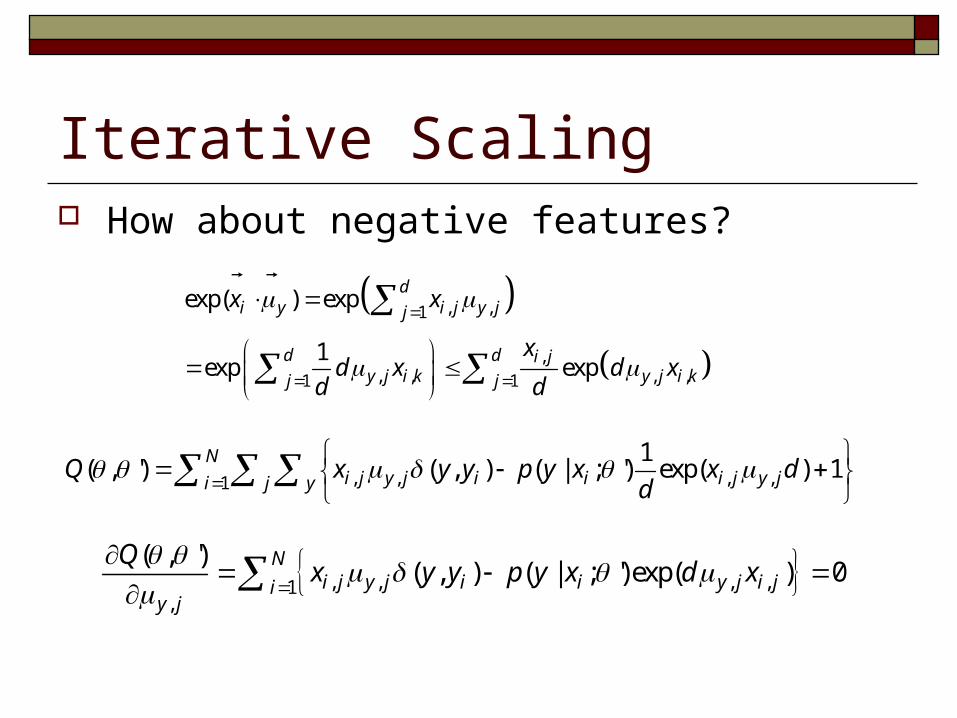
Iterative Scaling How about negative features?
, ,1
,, , , ,1 1
exp( ) exp
1exp exp
di y i j y jj
d d i jy j i k y j i kj j
x x
xd x d x
d d
, , , ,1
1( , ') ( , ) ( | ; ') exp( ) 1
Ni j y j i i i j y ji j y
Q x y y p y x x dd
, , , ,1,
( , ')( , ) ( | ; ') exp( ) 0
Ni j y j i i y j i ji
y j
Qx y y p y x d x

Faster Iterative Scaling The lower bound may not be tight given all the
coupling between weights is removed
A tighter bound can be derived by not fully decoupling the correlation between weights
,, , ,1
,1
( , ') ( , ) ( | ; ') exp( ) 1
( )
N i ji j y j i i i y ji j y
i
Ny ji j y
xQ x y y p y x g
g
q
Univariate functions!
,,, ,
,
( , ') , log ( | ) y j igi ji i j y j
j i y i yi
xQ y y x p y x e
g

Faster Iterative Scaling
Log-likelihood

Bad News You may feel great after the struggle of the derivation. However, is iterative scaling a true great idea? Given there have been so many studies in optimization, we
should try out existing methods.

Comparing Improved Iterative Scaling to Newton’s Method
Dataset Instances Features
Rule 29,602 246
Lex 42,509 135,182
Summary 24,044 198,467
Shallow 8,625,782 264,142
Dataset Iterations Time (s)
Rule 823 42.48
81 1.13
Lex 241 102.18
176 20.02
Summary 626 208.22
69 8.52
Shallow 3216 71053.12
421 2420.30
Limited-memory Quasi-Newton method
Improved iterative scaling
Try out the standard numerical methods before you get excited
about your algorithm