CLL: A Concurrent LanguageBuilt from Logical Principles

Deepak Garg

January, 2005CMU-CS-05-104

School of Computer ScienceCarnegie Mellon University

Pittsburgh, PA 15213

e-mail: dg+@cs.cmu.edu

This work has been partially supported by NSF Grant CCR-0306313 Efficient Logical Frameworks.

Keywords: Concurrent language, propositions as types, linear logic,logic programming, monad

Abstract

We present CLL, a concurrent programming language that symmetrically integrates functional and concur-rent logic programming. First, a core functional language is obtained from a proof-term assignment to avariant of intuitionistic linear logic, called FOMLL, via the Curry-Howard isomorphism. Next, we intro-duce a Chemical Abstract Machine (CHAM) whose molecules aretyped terms of this functional language.Rewrite rules for this CHAM are derived by augmenting proof-search rules for FOMLL with proof-terms.We show that this CHAM is a powerful concurrent language and that the linear connectives⊗, ∃, ⊕, (

and& correspond to process-calculi connectives for parallel composition, name restriction, internal choice,input prefixing and external choice respectively. We also demonstrate that communication and synchro-nization between CHAM terms can be performed through proof-search on the types of terms. Finally, weembed this CHAM as a construct in our functional language to allow interleaving functional and concurrentcomputation in CLL.

Contents

1 Introduction 3

2 fCLL: Functional Programming in CLL 42.1 Parallel Evaluation in Expressions . . . . . . . . . . . . . . . . .. . . . . . . . . . . . . . 132.2 Type-Safety . . . . . . . . . . . . . . . . . . . . . . . . . . . . . . . . . . . . .. . . . . . 132.3 Examples . . . . . . . . . . . . . . . . . . . . . . . . . . . . . . . . . . . . . . . .. . . . 17

3 lCLL: Concurrent Logic Programming in CLL 213.1 IntroducinglCLL . . . . . . . . . . . . . . . . . . . . . . . . . . . . . . . . . . . . . . . . 22

3.1.1 Structural Rules for Monadic Values and Synchronous Connectives . . . . . . . . . 233.1.2 Functional Rules for In-place Computation . . . . . . . . .. . . . . . . . . . . . . 253.1.3 Summary of Structural and Functional Rules . . . . . . . . .. . . . . . . . . . . . 253.1.4 Reaction Rules for Term Values and Asynchronous Connectives . . . . . . . . . . . 25

3.2 Programming Technique: Creating Private Names . . . . . . .. . . . . . . . . . . . . . . . 343.3 Example: Encoding theπ-calculus . . . . . . . . . . . . . . . . . . . . . . . . . . . . . . . 373.4 Types forlCLL CHAM Configurations . . . . . . . . . . . . . . . . . . . . . . . . . . . . . 403.5 Comparing process-calculi andlCLL . . . . . . . . . . . . . . . . . . . . . . . . . . . . . . 43

4 Full-CLL: Integrating fCLL and lCLL 444.1 Type-Safety . . . . . . . . . . . . . . . . . . . . . . . . . . . . . . . . . . . . .. . . . . . 46

5 Programming Techniques and Examples 475.1 Example: A Concurrent Fibonacci Program . . . . . . . . . . . . .. . . . . . . . . . . . . 475.2 Programming Technique: Buffered Asynchronous MessagePassing . . . . . . . . . . . . . 505.3 Example: Sieve of Eratosthenes . . . . . . . . . . . . . . . . . . . . .. . . . . . . . . . . 525.4 Implementing Buffered Asynchronous Message Passing using Functions . . . . . . . . . . . 555.5 Programming Technique: Synchronous Message Passing . .. . . . . . . . . . . . . . . . . 585.6 Example: One Cell Buffer . . . . . . . . . . . . . . . . . . . . . . . . . . .. . . . . . . . 605.7 Programming Technique: Synchronous Choices . . . . . . . . .. . . . . . . . . . . . . . . 60

5.7.1 Input-input Choice . . . . . . . . . . . . . . . . . . . . . . . . . . . . .. . . . . . 625.7.2 Output-output Choice . . . . . . . . . . . . . . . . . . . . . . . . . . .. . . . . . 635.7.3 Input-output Choice . . . . . . . . . . . . . . . . . . . . . . . . . . . .. . . . . . 64

5.8 Example: Read-Write Memory Cell . . . . . . . . . . . . . . . . . . . .. . . . . . . . . . 66

6 Discussion 67

Acknowledgment 68

References 68

1

2

1 Introduction

There are several ways to design a typed concurrent programming language. We may start from a syntax andoperational semantics for the terms of the language and add types in order to guarantee certain properties oftyped terms. Such properties include but are not limited to type-safety, deadlock freedom and several secu-rity properties. Examples of such languages are typed variants of theπ-calculus [20, 21, 22], join-calculus[16], CML [31] and Concurrent Haskell [28]. A completely different approach is to begin from a logic andlift it to a type system for a programming language using the Curry-Howard isomorphism. Proof-terms thatare witnesses for proofs in the logic become the terms of the programming language and proof normaliza-tion corresponds to the operational semantics. This approach has been successfully applied to the design offunctional programming languages. When we come to the concurrent paradigm where we allow creation ofprocesses executing in parallel and communicating with each other through one of several mechanisms likeshared memory, message queues or synchronization constructs like semaphores, monitors and events, at-tempts to design languages using the Curry-Howard isomorphism have mostly been theoretical. Most work[1, 2] in this direction is restricted to classical linear logic [18] and away from practice.1

A completely different meeting point for logic and concurrent programming is concurrent logic program-ming [34]. In this approach, one uses parallelism inherent in proof-search to design a logic programminglanguage which simulates concurrent process behavior. As is usual with all logic programming, only pred-icates and logical propositions play a part in programming and proof-terms are not used. Examples oflanguages of this kind are Concurrent Prolog[33] and FCP[23].

In this report, we use both the Curry-Howard isomorphism andproof-search to design a concurrent program-ming language from logical principles. We call this language CLL (Concurrent Linear Language). Our un-derlying logic is a first-order intuitionistic linear logicwhere all right synchronous connectives(⊗,⊕, 1,∃)are restricted to a monad. We refer to this logic as FOMLL (First-Order Monadic Linear Logic). Usinglinear logic to build the type system for a concurrent language seems a natural choice since processes arelinear entities. Ever since Girard’s first work on linear logic [18], deep connections between linear logicand concurrency have been suggested. For example, Abramskydevelops a concurrent computational inter-pretation of classical linear logic in [1]. FOMLL differs from the logic used by Abramsky in two essentialways. First, it is intuitionistic. Second, it is equipped with a monad. We use a monad in FOMLL becauseconcurrent computations haveeffectslike deadlocks and the monad separates pure functional terms from ef-fectful concurrent computations, enabling us to prove a type-safety theorem. This use of monads goes backto Moggi’s work [26] and similar uses of monads in concurrentlanguages like CML, Concurrent Haskelland Facile [31, 28, 17]. FOMLL has also been used in the Concurrent Logical Framework [35] which hasbeen used to represent several concurrent languages [12].

We design CLL in three steps. First, we construct a purely functional language (calledf CLL for functionalCLL) by adding proof-terms to FOMLL.f CLL admits basic linear functional constructs like abstraction,linear pairing, disjunctions, replication and recursive types, recursion and first-order dependent types. Italso allows parallelism - parts of programs may be evaluatedin parallel. However, there is no primitivefor communication between parallel processes. In the second step, we embedf CLL in a concurrent logicprogramming language calledlCLL (logic programmingCLL). The semantics of this logic programming

1Abramsky’s work [1] mentions some computational interpretations of intuitionistic linear logic also. However, these aresequential, not concurrent, interpretations and are not ofmuch interest in the context of this report.

3

language are presented as a Chemical Abstract Machine (CHAM) [4, 5, 7]. Molecules inlCLL CHAM con-figurations are terms off CLL annotated with their types. Rewrite rules for these CHAMconfigurations arederived from proof-search rules for FOMLL.lCLL differs from other logic programming languages in tworespects. First, we use the forward style of proof-search, not the traditional backward style. Second, proof-terms obtained during proof-search play a computational role in lCLL, which is not the case with other logicprogramming languages.lCLL is a powerful concurrent language that can encode all basic concurrencyconstructs like input and output processes, parallel composition for processes, choices, communication andeven n-way synchronization. In the third step, we embedlCLL back in f CLL as a language construct. Thismakes functional and concurrent logic programming symmetric in the language. SincelCLL configurationsproduce side effects like deadlocks, we restrict all CHAM configurations to the monad inf CLL. The resul-tant language is calledfull-CLL. We sometimes drop the prefix ‘full’ if it is clear from context.

An implementation of full-CLL in the Concurrent Logical Framework is available from the author’s home-page athttp://www.cs.cmu.edu/˜dg .

The contributions of this work are as follows. First, we showthat proof-search in logic has an interest-ing computational interpretation - it can be viewed as a procedure to link together programs to form largerprograms, which can then be executed. Working with FOMLL, wealso show how proof-search can be ex-ploited to add concurrency constructs to a programming language. Second, we demonstrate how functionaland logic programming can be symmetrically integrated in a single framework that allows interleaving func-tional computation and proof-search. Third, we establish that functional and concurrent programming canbe integrated symmetrically in a typed setting. In particular, we describe a method that allows concurrentcomputations inside functional programs to return non-trivial results, which can be used for further func-tional evaluation. Finally, we show that there is a correspondence between various concurrent constructslike parallel composition, name restriction, choices etc.and connectives of linear logic like⊗, ∃ and&.

Organization of the report. In section 2 we present the syntax, types and semantics off CLL. We provea type-safety result for this language and illustrate the expressiveness of our parallel construct with someexamples. In section 3 we build the concurrent logic programming lCLL and prove a type-preservationresult for it. lCLL is integrated withf CLL as a monadic construct to obtain full-CLL in section 4. Weprovea type-safety theorem for the whole language. A number of examples to illustrate the constructs in full-CLLare presented in section 5. Section 6 discusses related workand concludes the report.

2 fCLL: Functional Programming in CLL

Syntax. As mentioned in the introduction,f CLL is the functional core of CLL. It is designed from anunderlying logic (FOMLL), which under the Curry-Howard isomorphism corresponds to the type system.Hence the syntax of types is presented first. We assume a number of sorts, which are finite or infinite sets ofindex refinements (index terms are denoted byt). Index variables are denoted byi. See [36] for a detaileddescription of index refinements. Sort names are denoted byγ and its variants. Atomic type constructorsdenoted byP and its decorated variants havekindswhich are given by the grammar:

K ::= Type

| γ → K

We assume the existence of at least one infinite sort, namely the sort of channel names. This sort is called

4

chan. Channels are denoted by the letter k and its decorated variants. We assume the existence of someimplicit signature that gives the kinds of all atomic type constructors.

Types in CLL are derived from a variant of first-order intuitionistic linear logic [35, 13, 19] called FOMLL.We classify types into two categories based on the top level type constructor. If the top level constructor isatomic,&, →, ( or ∀, we call the typeasynchronousfollowing Andreoli[3]. In a sequent style presentationof linear logic, the right rules for asynchronous constructors are invertible, whereas their left rules are not.If the top constructor is!, ⊗, 1, ⊕, ∃ or µ, we call the typesynchronous. In sharp contrast to asynchronousconnectives, right rules for synchronous connectives are not invertible, whereas their left rules are. Allsynchronous types are restricted to a monad, whose constructor is denoted by{. . .}. Types are generated bythe following grammar:

A,B ::= (Asynchronous types)P t1 . . . tn (Atomic types)

| A&B (With or additive conjunction)| A→ B (Unrestricted implication)| A ( B (Linear implication)| {S} (Monadic type)| ∀i : γ.A (Universal quantification)

S ::= (Synchronous or monadic types)A (Base synchronous types)

| S1 ⊗ S2 (Tensor or multiplicative conjunction)| 1 (Unit of tensor)| S1 ⊕ S2 (Additive disjunction)| !A (Replication or exponential)| µα.S (Iso-recursive type)| ∃i : γ.S (Existential quantification)| α (Recursive type variable)

For proof-terms, we distinguish three classes of terms. “Pure” terms, sometimes simply called terms, de-noted byN , represent proofs of asynchronous types. Proofs of synchronous types are represented by twoclasses of syntax: monadic terms, denoted byM and expressions denoted byE. In general, monadic termsare constructive; they correspond to introduction rules ofsynchronous connectives. Expressions correspondto elimination terms and are the site of all parallelism inf CLL, as discussed later. The whole monad ispresented in a judgmental style [29]. The syntax of terms andexpressions in the language is given below.We assume the existence of three disjoint and infinite sets ofvariables - term variables denoted byx, y, . . .,recursion variables denoted byu, v, . . . and “choice” variables denoted byζ, ς, . . .

Terms, N ::= x | 〈N1,N2〉 | π1N | π2N | λx.N | λx.N | N1 N2 | N1 ˆN2 | {E}| Λi : γ.N | N [t]

Monadic terms, M ::= N |M1 ⊗M2 | 1 | inlM | inrM | !N| fold(M) | u | µu.M | [t,M ] |M1|ζM2

Expressions, E ::= M | let {p} = N in E | E1|ζE2

patterns, p ::= x | 1 | p1 ⊗ p2 | p1|ζp2 | !x | [i, p] | fold(p)

For elimination of the synchronous connectives,⊗,⊕, 1,∃ andµ, we use let constructions similar to [10]. Asopposed to usual elimination rules, which correspond to natural deduction style eliminations, the use of lets

5

gives rise to rules corresponding to left sequent rules of the sequent calculus. Choice variables{ζ, ς, . . .}are used to distinguish case branches for eliminating the connective⊕. For a detailed description of thistreatment see [10]. For clarity, we sometimes annotate bound variables andfold constructs with their types.

Type System. We use four contexts in our typing judgments:Σ (index variable context),Γ (unrestrictedcontext),∆ (linear context) andΨ (recursion context). The grammars generating these contexts are:

Σ ::= · | Σ, i : γΓ ::= · | Γ, x : A∆ ::= · | ∆, p : S if p⇒ SΨ ::= · | Ψ, u : S

The judgmentp ⇒ S, read as “p matchesS” is described in figure 1. Subsequently, it is assumed thatwheneverp : S occurs in a context,p ⇒ S. Given a context, the variables it defines are called its definedvariables,dv . Related concepts are definedlinear variables,dlv and definedindexvariables,div . Theseare precisely described in figure 2. Given a contextΣ;Γ;∆;Ψ, we assume that the setsdv(Γ), dv(∆),dv(Ψ), div(Σ) anddiv(∆) are all pairwise disjoint. We use four typing judgments in our type system:

Σ;Γ;∆;Ψ ` N : A

Σ;Γ;∆;Ψ ` M # S

Σ;Γ;∆;Ψ ` E ÷ S

Σ ` t : γ

The last judgment is external to the language and we do not specify how we check the well-sortedness ofrefinement terms. We simply assume the following propertiesof this judgment:

1. Substitution: IfΣ ` t : γ andΣ, i : γ ` t′ : γ′, thenΣ ` t′ [t/i] : γ′.

2. Weakening: IfΣ ` t : γ, thenΣ, i : γ ` t : γ.

3. Strengthening: IfΣ, i : γ ` t : γ andi 6∈ t, thenΣ ` t : γ.

The other three typing judgments assume that all types inΓ,∆ andΨ are well-formed with respect to therefinement term contextΣ. The typeP t1 . . . tn is well formed inΣ if Kind(P ) = γ1 . . . γn → Type andΣ ` ti : γi for i = 1 . . . n. The well formedness of other types is obtained by lifting this relation in thestandard way. The typing rules forf CLL are given in figures 3, 4, 5 and 6. It may be observed here thatthere is no⊕ − L rule for terms similar to the rules⊕ − LM and⊕ − LE (see figure 6) because we do notallow choice branches in pure terms. This is done because we found that in practice choice branches in pureterms are never needed.

Operational Semantics. We use call-by-value semantics forf CLL. However, certain constructs have to beevaluated lazily due to linearity constraints and the presence of a monad. For example, pairs at the levelof terms have to be lazy because the two components of a pair share the same linear resources and onlythe component that will be used in the remaining computationshould be evaluated. Thus evaluation ofthe components of a pair is postponed till one of the components is projected. The monad is also a lazyconstruct because it encloses expressions, whose evaluation can have side effects. We do not evaluate thebody of a functional abstraction (λx.N , λx.N andΛi.N ), since evaluation is restricted toclosedterms,

6

x⇒ A !x⇒!A

1 ⇒ 1p⇒ S

[i1, p] ⇒ ∃i2 : γ.S

p1 ⇒ S1 p2 ⇒ S2

p1 ⊗ p2 ⇒ S1 ⊗ S2

p⇒ S(µα.S(α))

fold(p) ⇒ µα.S(α)

p1 ⇒ S1 p2 ⇒ S2

p1|ζp2 ⇒ S1 ⊕ S2

Figure 1: p⇒ S

dv(x) = {x} dv(!x) = {x}dv(p1 ⊗ p2) = dv(p1) ∪ dv(p2) dv(1) = φdv(p1|ζp2) = {ζ} ∪ dv(p1) ∪ dv(p2) dv([i, p]) = dv(p)dv(fold(p)) = dv(p)

dv(·) = φ dv(Γ, x : A) = dv(Γ) ∪ {x}dv(∆, p : S) = dv(∆) ∪ dv(p) dv(Ψ, u : S) = dv(Ψ) ∪ {u}dv(Σ) = φ

dlv(x) = {x} dlv(!x) = φdlv(p1 ⊗ p2) = dlv(p1) ∪ dlv(p2) dlv(1) = φdlv(p1|ζp2) = dlv(p1) ∪ dlv(p2) dlv([i, p]) = dlv(p)dlv(fold(p)) = dlv(p)

dlv(·) = φ dlv(∆, p : S) = dlv(∆) ∪ dlv(p)dlv(Γ) = φ dlv(Ψ) = φdlv(Σ) = φ

div(x) = φ div(!x) = φdiv(p1 ⊗ p2) = div(p1) ∪ div(p2) div(1) = φdiv(p1|ζp2) = div(p1) ∪ div(p2) div([i, p]) = {i}div(fold(p)) = div(p)

div(·) = φ div(∆, p : S) = div(∆) ∪ div(p)div(Γ) = φ div(Ψ) = φdiv(Ψ) = φ div(Σ) = dom(Σ)

Figure 2: Defined variables of patterns and contexts

7

Hyp1

Σ;Γ;x : A; Ψ ` x : AHyp2

Σ;Γ, x : A; ·; Ψ ` x : A

Σ;Γ;∆;Ψ ` N1 : A1 Σ;Γ;∆;Ψ ` N2 : A2&-I

Σ;Γ;∆;Ψ ` 〈N1,N2〉 : A1&A2

Σ;Γ;∆;Ψ ` N : A1&A2&-E1

Σ;Γ;∆;Ψ ` π1N : A1

Σ;Γ;∆;Ψ ` N : A1&A2&-E2

Σ;Γ;∆;Ψ ` π2N : A2

Σ;Γ, x : A;∆;Ψ ` N : B→-I

Σ;Γ;∆;Ψ ` λx.N : A→ B

Σ;Γ;∆, x : A; Ψ ` N : B(-I

Σ;Γ;∆;Ψ ` λx.N : A ( B

Σ;Γ;∆;Ψ ` N1 : A→ B Σ;Γ; ·; Ψ ` N2 : A→-E

Σ;Γ;∆;Ψ ` N1 N2 : B

Σ;Γ;∆1; Ψ ` N1 : A ( B Σ;Γ;∆2; Ψ ` N2 : A(-E

Σ;Γ;∆1,∆2; Ψ ` N1 ˆN2 : B

Σ;Γ;∆;Ψ ` E ÷ S{}-I

Σ;Γ;∆;Ψ ` {E} : {S}

Σ, i : γ; Γ;∆;Ψ ` N : A∀-I

Σ;Γ;∆;Ψ ` Λi : γ.N : ∀i : γ.A

Σ;Γ;∆;Ψ ` N : ∀i : γ.A(i) Σ ` t : γ∀-E

Σ;Γ;∆;Ψ ` N [t] : A(t)

Figure 3: Type system for Terms

8

Σ;Γ;∆;Ψ ` N : A: #

Σ;Γ;∆;Ψ ` N # A

Hyp3

Σ;Γ; ·; Ψ, u : S ` u # S1-R

Σ;Γ; ·; Ψ ` 1 # 1

Σ;Γ;∆1; Ψ ` M1 # S1 Σ;Γ;∆2; Ψ ` M2 # S2⊗-R

Σ;Γ;∆1,∆2; Ψ ` M1 ⊗M2 # S1 ⊗ S2

Σ;Γ;∆;Ψ ` M # S1⊕-R1

Σ;Γ;∆;Ψ ` inlM # S1 ⊕ S2

Σ;Γ;∆;Ψ ` M # S2⊕-R2

Σ;Γ;∆;Ψ ` inrM # S1 ⊕ S2

Σ;Γ; ·; Ψ ` N : A!-R

Σ;Γ; ·; Ψ ` !N # !A

S = µα.S′(α) Σ; Γ;∆;Ψ ` M # S′(S)fold-R

Σ;Γ;∆;Ψ ` fold(M) # S

Σ;Γ; ·; Ψ, u : S ` M # Srec

Σ;Γ; ·; Ψ ` µu.M # S

Σ;Γ;∆;Ψ ` M # S(t) Σ ` t : γ∃-R

Σ;Γ;∆;Ψ ` [t,M ] # ∃i : γ.S(i)

Figure 4: Type system for Monadic Terms

Σ;Γ;∆;Ψ ` M # S# ÷

Σ;Γ;∆;Ψ ` M ÷ S

Σ;Γ;∆1; Ψ ` N : {S} Σ;Γ;∆2, p : S; Ψ ` E ÷ S′

{}-E

Σ;Γ;∆1,∆2; Ψ ` let {p} = N in E ÷ S′

Figure 5: Type system for Expressions

9

T % Z ::= N : A |M # S | E ÷ S

Σ;Γ, x : A;∆;Ψ ` T % Z!-L

Σ;Γ;∆, !x :!A; Ψ ` T % Z

Σ;Γ;∆, p1 : S1, p2 : S2; Ψ ` T % Z⊗-L

Σ;Γ;∆, p1 ⊗ p2 : S1 ⊗ S2; Ψ ` T % Z

Σ;Γ;∆;Ψ ` T % Z1-L

Σ;Γ;∆, 1 : 1;Ψ ` T % Z

Σ;Γ;∆, p : S(µα.S(α));Ψ ` T % Zfold-L

Σ;Γ;∆, fold(p) : µα.S(α);Ψ ` T % Z

Σ, i : γ; Γ;∆, p : S; Ψ ` T % Z∃-L (i 6∈ Σ, Γ, ∆, p, Ψ, Z)

Σ;Γ;∆, [i, p] : ∃i : γ.S; Ψ ` T % Z

Σ;Γ;∆, p1 : S1; Ψ ` M1 # S Σ;Γ;∆, p2 : S2; Ψ ` M2 # S⊕-LM

Σ;Γ;∆, p1|ζp2 : S1 ⊕ S2; Ψ ` M1|ζM2 # S

Σ;Γ;∆, p1 : S1; Ψ ` E1 ÷ S Σ;Γ;∆, p2 : S2; Ψ ` E2 ÷ S⊕-LE

Σ;Γ;∆, p1|ζp2 : S1 ⊕ S2; Ψ ` E1|ζE2 ÷ S

Figure 6: Type system : Left rules for patterns

monadic terms and expressions only. We call a term, monadic term or expression closed if it has no freevariables. Apart from these restrictions, all other constructs inf CLL (⊗, inl, inr, !, fold and existentials)are evaluated eagerly. Values forf CLL are described below:

Term values, V ::= λx.N | λx.N | {E} | 〈N1,N2〉 | Λi.NMonadic values, Mv ::= V |Mv1

⊗Mv2| 1 | inlMv | inrMv | !V | foldMv | [t,Mv]

There are no values at the expression level, because expressions evaluate to monadic values. We define twooperations on terms, monadic terms and expressions off CLL: leftζ andrightζ , which are the left andright case branches for the choice variableζ, respectively. Figure 7 defines some of the interesting casesof these operations. The definitions for the remaining syntactic constructors are obtained by lifting thesedefinitions homomorphically. Thusleftζ(x) = x, leftζ(λx.N) = λx.leftζ(N), leftζ(N1 N2) =leftζ(N1) leftζ(N2), leftζ(M1 ⊗M2) = leftζ(M1)⊗ leftζ(M2), leftζ({E}) = {leftζ(E)}, etc.The result of substituting a monadic valueMv for a patternp of the corresponding “shape” in a programT(subst(M/p, T )) is given in figure 8. This substitution is defined by induction on the structure of the pat-ternp. The base substitutions[V/x] and[t/i] are the usual capture avoiding substitutions for free variablesand free index variables respectively.

The call-by-value evaluation rules forf CLL are given in figures 9, 10 and 11. We use three reductionjudgments -N → N ′, M 7→ M ′ andE ↪→ E′. The rules are standard. We allow reductions ofM1

andM2 to interleave when we reduceM1 ⊗M2. Thus the two components of a tensor may be evaluatedin parallel. For reasons mentioned earlier, pairs and the monad at the term level are evaluated lazily. Thereduction rules for abstractions and applications are standard call-by-value.

10

leftζ(M1|ζM2) = M1 leftζ(M1|εM2) = leftζ(M1)|εleftζ(M2) ε 6= ζleftζ(E1|ζE2) = E1 leftζ(E1|εE2) = leftζ(E1)|εleftζ(E2) ε 6= ζ

leftζ(let {p} = N in E) = (let {p} = leftζ(N) in leftζ(E)) (ζ 6∈ dv(p))

rightζ(M1|ζM2) = M2 rightζ(M1|εM2) = rightζ(M1)|εrightζ(M2) ε 6= ζ

rightζ(E1|ζE2) = E2 rightζ(E1|εE2) = rightζ(E1)|εrightζ(E2) ε 6= ζ

rightζ(let {p} = N in E) = (let {p} = rightζ(N) in rightζ(E)) (ζ 6∈ dv(p))

Figure 7: Choice projections forf CLL

T ::= N |M | E

subst(1/1, T ) = T subst(V/x, T ) = T [V/x]subst(!V/!x, T ) = subst(V/x, T ) subst([t,Mv ]/[i, p], T ) = subst(Mv/p, T [t/i])

subst(inlMv/(p1|ζp2), T ) = subst(Mv/p1, leftζ(T ))

subst(inrMv/(p1|ζp2), T ) = subst(Mv/p2, rightζ(T ))

subst(Mv1⊗Mv2

/p1 ⊗ p2, T ) = subst(Mv2/p2, subst(Mv1

/p1, T ))

subst(fold(Mv)/fold(p), T ) = subst(Mv/p, T )

Figure 8: Substitution of monadic values for patterns

11

N → N ′→ π1

π1 N → π1N′

N → N ′→ π2

π2 N → π2N′

→ 〈〉π1

π1 〈N1, N2〉 → N1

→ 〈〉π2

π2 〈N1,N2〉 → N2

N1 → N ′1

→ APP1

N1 N2 → N ′1 N2

N2 → N ′2

→ APP2

V N2 → V N ′2

→ λAPP

(λx.N) V → N [V/x]

N1 → N ′1

→ LAPP1

N1 ˆN2 → N ′1 ˆN2

N2 → N ′2

→ LAPP2

V ˆN2 → V ˆN ′2

→ λLAPP

(λx.N)ˆV → N [V/x]

N → N ′→ ∀

N [t] → N ′ [t]→ ΛAPP

(Λi : γ.N) [t] → N [t/i]

Figure 9: Reduction for terms,N → N ′

N → N ′→7→

N 7→ N ′N → N ′

7→!

!N 7→ !N ′

M1 7→ M ′1

7→ ⊗1

M1 ⊗M2 7→ M ′1 ⊗M2

M2 7→ M ′2

7→ ⊗2

M1 ⊗M2 7→ M1 ⊗M ′2

M 7→ M ′7→ ⊕1

inlM 7→ inlM ′M 7→ M ′

7→ ⊕2

inrM 7→ inrM ′

M 7→ M ′7→ F OLD

foldM 7→ foldM ′

M 7→ M ′7→ ∃

[t,M ] 7→ [t,M ′]

7→ µ

µu.M 7→ M [µu.M/u]

Figure 10: Reduction for monadic terms,M 7→ M ′

M 7→ M ′7→↪→

M ↪→ M ′↪→ LETRED

let {p} = {Mv} in E ↪→ subst(Mv/p,E)

N → N ′↪→ LET1

let {p} = N in E ↪→ let {p} = N ′ in E

E ↪→ E′↪→ LET2

let {p} = {E} in E1 ↪→ let {p} = {E′} in E1

Figure 11: Reduction for expressions,E ↪→ E′

12

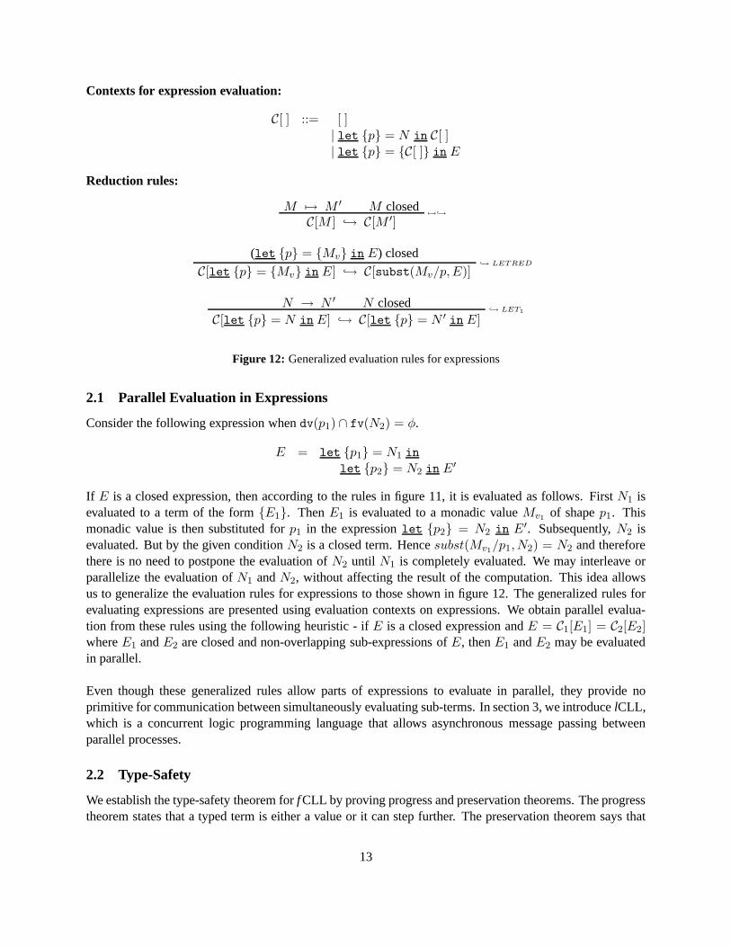
Contexts for expression evaluation:

C[ ] ::= [ ]| let {p} = N in C[ ]| let {p} = {C[ ]} in E

Reduction rules:

M 7→ M ′ M closed7→↪→

C[M ] ↪→ C[M ′]

(let {p} = {Mv} in E) closed↪→ LETRED

C[let {p} = {Mv} in E] ↪→ C[subst(Mv/p,E)]

N → N ′ N closed↪→ LET1

C[let {p} = N in E] ↪→ C[let {p} = N ′ in E]

Figure 12: Generalized evaluation rules for expressions

2.1 Parallel Evaluation in Expressions

Consider the following expression whendv(p1) ∩ fv(N2) = φ.

E = let {p1} = N1 in

let {p2} = N2 in E′

If E is a closed expression, then according to the rules in figure 11, it is evaluated as follows. FirstN1 isevaluated to a term of the form{E1}. ThenE1 is evaluated to a monadic valueMv1

of shapep1. Thismonadic value is then substituted forp1 in the expressionlet {p2} = N2 in E′. Subsequently,N2 isevaluated. But by the given conditionN2 is a closed term. Hencesubst(Mv1

/p1,N2) = N2 and thereforethere is no need to postpone the evaluation ofN2 until N1 is completely evaluated. We may interleave orparallelize the evaluation ofN1 andN2, without affecting the result of the computation. This ideaallowsus to generalize the evaluation rules for expressions to those shown in figure 12. The generalized rules forevaluating expressions are presented using evaluation contexts on expressions. We obtain parallel evalua-tion from these rules using the following heuristic - ifE is a closed expression andE = C1[E1] = C2[E2]whereE1 andE2 are closed and non-overlapping sub-expressions ofE, thenE1 andE2 may be evaluatedin parallel.

Even though these generalized rules allow parts of expressions to evaluate in parallel, they provide noprimitive for communication between simultaneously evaluating sub-terms. In section 3, we introducelCLL,which is a concurrent logic programming language that allows asynchronous message passing betweenparallel processes.

2.2 Type-Safety

We establish the type-safety theorem forf CLL by proving progress and preservation theorems. The progresstheorem states that a typed term is either a value or it can step further. The preservation theorem says that

13

⇐= −1

Σ;Γ;∆ ⇐= Σ;Γ;∆, 1 : 1⇐= −!

Σ;Γ, x : A;∆ ⇐= Σ;Γ;∆, !x :!A

⇐= −⊗

Σ;Γ;∆, p1 : S1, p2 : S2 ⇐= Σ;Γ;∆, p1 ⊗ p2 : S1 ⊗ S2

⇐= −∃

Σ, i : γ; Γ;∆, p : S(i) ⇐= Σ;Γ;∆, [i, p] : ∃i : γ.S(i)

⇐= −fold

Σ;Γ;∆, p : S(µα.S(α)) ⇐= Σ;Γ;∆, fold(p) : µα.S(α)

⇐= −REF

Σ;Γ;∆ ⇐= Σ;Γ;∆Σ;Γ;∆ ⇐= Σ′; Γ′;∆′ Σ′; Γ′;∆′ ⇐= Σ′′; Γ′′;∆′′

⇐= −TRANS

Σ;Γ;∆ ⇐= Σ′′; Γ′′;∆′′

Figure 13: Context entailment,Σ; Γ; ∆ ⇐= Σ′; Γ′; ∆′

reduction of a typed term under the evaluation rules preserves its type. Together these two implytype-safetyi.e. any typed term either evaluates to a value or diverges indefinitely. In order to establish these theorems,we need a few results.

Notation 1. We useT % Z to denote any ofN : A,M # S orE ÷ S.

Definition 1 (Context Entailment). The relationΣ;Γ;∆ ⇐= Σ′; Γ′;∆′, read asΣ;Γ;∆ entailsΣ′; Γ′;∆′,is shown in figure 13.

Lemma 1 (⇐= properties).

1. If Σ;Γ;∆ ⇐= Σ′; Γ′;∆′, thenΣ ⊇ Σ′ andΓ ⊇ Γ′.

2. If Σ;Γ;∆ ⇐= Σ′; Γ′;∆′, then

(a) dv(Γ) ∪ dv(∆) = dv(Γ′) ∪ dv(∆′)

(b) dlv(∆) = dlv(∆′)

(c) div(Σ) ∪ div(∆) = div(Σ′) ∪ div(∆′)

3. If D :: Σ; Γ;∆;Ψ ` T % Z andΣ;Γ;∆ ⇐= Σ′; Γ′;∆′, thenD can beextendedto a derivationD′ :: Σ′; Γ′;∆′; Ψ ` T % Z using the rules⊗− L, 1 − L, ∃ − L, ! − L andfold− L only.

4. (Weakening) IfΣ;Γ;∆ ⇐= Σ′; Γ′;∆′, then

(a) Σ,Σ′′; Γ;∆ ⇐= Σ′,Σ′′; Γ′;∆′

(b) Σ;Γ,Γ′′;∆ ⇐= Σ′; Γ′,Γ′′;∆′

(c) Σ;Γ;∆,∆′′ ⇐= Σ′; Γ′;∆′,∆′′

Proof. In each case by induction on the given derivationΣ;Γ;∆ ⇐= Σ′; Γ′;∆′.

Definition 2 (Height of a derivation). The height of a derivationD, height(D) is defined to be the lengthof longest path from the conclusion to any leaf.

14

Lemma 2 (Weakening). If Σ;Γ;∆;Ψ ` ψ, then

1. Σ, i : γ; Γ;∆;Ψ ` ψ.

2. Σ;Γ, x : A;∆;Ψ ` ψ.

3. Σ;Γ;∆;Ψ, u : S ` ψ.

Proof. By induction on the given derivation.

Lemma 3 (Left inversion).

1. If Σ;Γ;∆, p : 1;Ψ ` ψ, thenp = 1 andΣ;Γ;∆;Ψ ` ψ.

2. If Σ;Γ;∆; p :!A; Ψ ` ψ, thenp =!x andΣ;Γ, x : A;∆;Ψ ` ψ.

3. If Σ;Γ;∆, p : A; Ψ ` ψ, thenp = x.

4. If Σ;Γ;∆, p : S1 ⊗ S2; Ψ ` ψ, thenp = p1 ⊗ p2 andΣ;Γ;∆, p1 : S1, p2 : S2; Ψ ` ψ.

5. If Σ;Γ;∆, p : ∃i : γ.S; Ψ ` ψ, thenp = [i, p1] andΣ, i : γ; Γ;∆, p1 : S; Ψ ` ψ.

6. If Σ;Γ;∆, p : S1 ⊕ S2; Ψ ` ψ, thenp = p1|ζp2, Σ;Γ;∆, p1 : S1; Ψ ` leftζ(ψ) andΣ;Γ;∆, p2 :S2; Ψ ` rightζ(ψ). (leftζ(N : A) = leftζ(N) : A, etc.)

7. If Σ;Γ;∆, p : µα.S(α);Ψ ` ψ, thenp = fold(p′) andΣ;Γ;∆, p′ : S(µα.S(α));Ψ ` ψ.

Proof. Each statement may be separately proved by induction on thegiven typing derivation.

Lemma 4 (Strong right value inversion).

1. If D :: Σ; Γ;∆;Ψ ` V : A → B then V = λx.N and there is a derivationD′ :: Σ; Γ, x :A;∆;Ψ ` N : B with height(D′) ≤ height(D).

2. If D :: Σ; Γ;∆;Ψ ` V : A ( B thenV = λx.N and there is a derivationD′ :: Σ; Γ;∆, x :A; Ψ ` N : B with height(D′) ≤ height(D).

3. If D :: Σ; Γ;∆;Ψ ` V : A&B thenV = 〈N1,N2〉 and there are derivationsD1 :: Σ; Γ;∆;Ψ ` N1 :A andD2 :: Σ; Γ;∆;Ψ ` N2 : B with height(D1) ≤ height(D) andheight(D2) ≤ height(D).

4. If D :: Σ; Γ;∆;Ψ ` V : {S} thenV = {E} and there is a derivationD′ :: Σ; Γ;∆;Ψ ` E ÷ Swith height(D′) ≤ height(D).

5. If D :: Σ; Γ;∆;Ψ ` V : ∀i : γ.A(i), i 6∈ Σ thenV = Λi : γ.N(i) and there is a derivationD′ :: Σ, i : γ; Γ;∆;Ψ ` N(i) : A(i) with height(D′) ≤ height(D).

Proof. Each statement can be proved separately by induction on thegiven typing derivation.

Lemma 5 (Right monadic value inversion).

1. If Σ;Γ;∆;Ψ ` Mv # A, thenMv = V andΣ;Γ;∆;Ψ ` V : A.

15

2. If Σ;Γ;∆;Ψ ` Mv # !A, thenMv =!V and for someΣ′ and Γ′, Σ′; Γ′; ·; Ψ ` V : A andΣ′; Γ′; · ⇐= Σ;Γ;∆.

3. If Σ;Γ;∆;Ψ ` Mv # S1 ⊗ S2, thenMv = Mv1⊗Mv2

and for someΣ′,Γ′,∆′1,∆

′2, the following

three hold:

(a) Σ′; Γ′;∆′1,∆

′2 ⇐= Σ;Γ;∆

(b) Σ′; Γ′;∆′1; Ψ ` Mv1

# S1

(c) Σ′; Γ′;∆′2; Ψ ` Mv2

# S2

4. If Σ;Γ;∆;Ψ ` Mv # 1, thenMv = 1 and for someΣ′ andΓ′, Σ′; Γ′; · ⇐= Σ;Γ;∆.

5. If Σ;Γ;∆;Ψ ` Mv # S1 ⊕ S2, then one of the following holds

(a) Mv = inlM ′v andΣ;Γ;∆;Ψ ` M ′

v # S1

(b) Mv = inrM ′v andΣ;Γ;∆;Ψ ` M ′

v # S2

6. If Σ;Γ;∆;Ψ ` Mv # ∃i : γ.S(i), thenMv = [t,M ′v] and for someΣ′, Γ′ and∆′, the following

three hold:

(a) Σ′; Γ′;∆′ ⇐= Σ;Γ;∆

(b) Σ′ ` t : γ

(c) Σ′; Γ′;∆′; Ψ ` M ′v # S(t)

7. If Σ;Γ;∆;Ψ ` Mv # µα.S(α), thenMv = fold(M ′v) andΣ;Γ;∆;Ψ ` M ′

v # S(µα.S(α)).

Proof. In each case by induction on the given typing derivation.

Lemma 6 (Strong right inversion for expressions).

1. If D :: Σ; Γ;∆;Ψ ` M ÷ S, then there existsD′ :: Σ; Γ;∆;Ψ ` M # S with height(D′) ≤height(D).

2. If D :: Σ; Γ;∆;Ψ ` let {p} = N in E ÷ S′, then there existΣ′,Γ′,∆′1,∆

′2, S,D1,D2 such that

(a) Σ′; Γ′;∆′1,∆

′2 ⇐= Σ;Γ;∆

(b) D1 :: Σ′; Γ′;∆′1; Ψ ` N : {S} andheight(D1) ≤ height(D)

(c) D2 :: Σ′; Γ′;∆′2, p : S; Ψ ` E ÷ S′ andheight(D2) ≤ height(D)

Proof. By induction on the given typing derivation.

Lemma 7 (Substitution).

1. If D :: Σ; Γ;∆;Ψ ` V : A andD′ :: Σ; Γ;∆′, x : A; Ψ ` T %Z, thenΣ;Γ;∆,∆′; Ψ ` T [V/x] %Z.

2. If Σ ` t : γ andD′ :: Σ, i : γ; Γ;∆;Ψ ` T (i) %Z(i), thenΣ;Γ[t/i];∆[t/i]; Ψ[t/i] ` T (t) %Z(t).

3. If D :: Σ; Γ;∆;Ψ ` Mv # S andD′ :: Σ; Γ;∆′, p : S; Ψ ` T % Z, thenΣ;Γ;∆,∆′; Ψ ` subst(Mv/p, T ) % Z.

16

4. If D :: Σ; Γ; .; Ψ ` V : A andD′ :: Σ; Γ, x : A;∆′; Ψ ` T % Z, thenΣ;Γ;∆′; Ψ ` T [V/x] % Z.

5. If D :: Σ; Γ; .; Ψ ` M # S andD′ :: Σ; Γ;∆′; Ψ, u : S ` T %Z, thenΣ;Γ;∆′; Ψ ` T [M/u] %Z.

Proof. Statements (1), (2), (4) and (5) can be proved by induction on derivationD′. To prove (3), we useinduction on the derivationD, lemmas 2 and 3 and statements (1) and (2).

Lemma 8 (Preservation).

1. If Σ;Γ;∆;Ψ ` N : A andN → N ′, thenΣ;Γ;∆;Ψ ` N ′ : A.

2. If Σ;Γ;∆;Ψ ` M # S andM 7→ M ′, thenΣ;Γ;∆;Ψ ` M ′ # S.

3. If Σ;Γ;∆;Ψ ` E ÷ S andE ↪→ E′, thenΣ;Γ;∆;Ψ ` E′ ÷ S.

Proof. By simultaneous induction on the height of the given typingderivation, using lemmas 7, 6 and 4. Forthe case of expressions, we perform a sub-induction on the evaluation contextC[ ] and use lemma 6.

Lemma 9 (Progress).

1. If Σ; ·; ·; · ` N : A, then eitherN = V or for someN ′,N → N ′.

2. If Σ; ·; ·; · ` M # S, then eitherM = Mv or for someM ′,M 7→ M ′.

3. If Σ; ·; ·; · ` E ÷ S, then eitherE = Mv or for someE′,E ↪→ E′.

Proof. By induction on the given typing derivation.

Theorem 1 (Type-Safety).

1. If Σ; ·; ·; · ` N : A andN →∗ N ′, then eitherN ′ = V or there existsN ′′ such thatN ′ → N ′′.

2. If Σ; ·; ·; · ` M # S andM 7→∗ M ′, then eitherM ′ = Mv or there existsM ′′ such thatM ′ 7→M ′′.

3. If Σ; ·; ·; · ` E ÷ S andE ↪→∗ E′, then eitherE′ = Mv or there existsE′′ such thatE′ ↪→ E′′.

Proof. By induction on the number of steps in the reduction. The statement at the base case (no reduction)is the same as the progress lemma (lemma 9). For the inductionstep, we use preservation (lemma 8).

2.3 Examples

In this section we explain program construction inf CLL through a number of examples. We present theseexamples in ML-like syntax. We assume that we have named and recursive functions, conditionals anddatatype constructions at the term level, which may be addedto f CLL presented above in a straightforwardmanner.

Divide and Conquer. Our first example is a general divide and conquer program. Let us suppose we have atypeP of problems and a typeA of solutions. A general divide and conquer method assumes the followinginput functions:

1. divide : P → P × P that divides a given problem into two subproblems, each of which is strictlysmaller than the original.

17

2. istrivial : P → bool that decides if the input problem is at its base case.

3. solve : P → A that returns the solution to a base case problem.

4. merge : A → A → A that combines solutions of two subproblems obtained usingdivide into asolution to the original problem.

In f CLL, we have no product type (which would be present in a non-linear language). So we encodethe product type asA × B = {!A ⊗ !B}. Then we have the following divide and conquer function,divAndConquer:

divAndConquer =λ(divide) : P → {!P⊗!P}. λ(istrivial) : P → bool.λ(solve) : P → {!A}. λ(merge) : A→ A→ {!A}. λp : P .if (istrivial p) then solve pelse

{let {!p1⊗!p2} = divide p inlet {!s1} = divAndConquer divide istrivial solve merge p1 in

let {!s2} = divAndConquer divide istrivial solve merge p2 in

let {!s} = merge s1 s2 in!s

}

The return type ofdivAndConquer is {!A}. Observe that in this program, the twolet eliminations corre-sponding to the two recursive calls may occur in parallel i.e. the termsdivAndConquer divide istrivialsolve merge p1 anddivAndConquer divide istrivial solve merge p2 can be evaluated simultaneously.This is because the second term does not use the variables1. Therefore the program above attains the paral-lelism that is expected in a divide and conquer approach.

Bellman-Ford algorithm . We now present a parallel implementation of Bellman-Ford algorithm for singlesource shortest paths in directed, non-negative edge-weighted graphs. Assume that a directed graphG hasn vertices, numbered1, . . . , n. For each vertex we have a list of incoming edges called the adjacency listof the vertex. Each element of the adjacency list is a pair, the first member of which is an integer, whichis the source vertex of the edge and the second member is a non-negative real number, which is the weightof the edge. The whole graph is represented as a list of adjacency lists, one adjacency list for each vertex.During the course of the algorithm, we have approximations of shortest distance from the source vertex toeach vertex. These are stored as a list of reals. The type of this list is calleddistlist .

type distlist = {!real} listtype adjlist = {!int⊗ !real} listtype edgelist = {!adjlist} list

The following function finds the ith element of a list l.

18

val find: ′a list → int → ′afind =

λl: ′a list. λi:int.if ( i = 1) then head( l) else find(tail( l))( i− 1)

The main routine of the Bellman-Ford algorithm is a relaxation procedure that takes as input a vertex,v(which in our case is completely represented by the adjacency list, al. The exact vertex number of thevertex is immaterial), a presently known approximation of shortest distances to all vertices from the source(calleddl), the present known approximation of the shortest distancefrom the source tov and returns a newapproximation to the shortest distance from source tov.

val relax: adjlist → distlist → real → {!real}relax =

λ( al):adjlist. λ( dl):distlist. λd:real.case ( al) of

[] => {!d}| ( a :: al) =>

{let {!v⊗!w} = a inlet {!d′} = find dl v inlet {!d′′} = relax al dl d in

!min( d′′, d′ + w)}

The callsfind dl v and relax al dl d can be reduced in parallel in the above function. The mainloop of the Bellman-Ford algorithm is a functionrelaxall , that applies the functionrelax to all thevertices. To make the code simpler, we assume that this function actually takes as argumenttwo copiesofthe distance list. To make the code more presentable, we droptheλ-calculus notation and use standard ML’sfun notation.

val relaxall: edgelist → distlist → distlist → {!distlist}fun relaxall [] [] dl = {![] }| relaxall ( al :: el)( d :: dl′)( dl) =

{let {!al′} = al inlet {!d′} = d inlet {!d1} = relax al′ dl d′ inlet {!l} = relaxall el dl′ dl in

!({!d1} :: l)}

19

In the above function, the callsrelax al′ dl d′ andrelaxall el dl′ dl can be reduced in parallel.This results in simultaneous relaxation for the whole graph.

Suppose now that our source vertex is the vertex1. Then we can initialize thedistlist to the value[0,∞, . . . ,∞]. Using this initial value of thedistlist , we iterate the functionrelaxall n times. Theresultant value ofdistlist is the list of minimum distances from the source (vertex 1) toall the othervertices. The functionBF below takes as input a graph (in the form of anedgelist ) and returns theminimum distances to all vertices from the vertex 1.

fun BF (el: edgelist) =(* makedistlist: int → {!distlist} *)let fun makedistlist 0 = {![]}

| makedistlist k ={

let {!l} = makelist (k − 1)in

!({!∞} :: l)}

(* loop: int → distlist → {!distlist} *)fun loop 0 dl = {!dl}| loop k dl =

{let {!dl′} = relaxall el dl dlin

loop (k − 1) dl′

}

(* length: ’a list → {!int} *)fun length [] = {!0}| length ( x :: l) =

{let {!len} = length (l)in

!(1 + len)}

in{

let {!n} = length el inlet {!l} = makedistlist (n− 1) inlet {!dl} = loop n ({!0} :: l) in

!dl}end

20

3 lCLL: Concurrent Logic Programming in CLL

As mentioned in the introduction, an alternate paradigm used for concurrent languages is concurrent logicprogramming [34]. In this paradigm, proof-search in logic simulates computation and assignment to vari-ables as well as communication are implemented through unification. Concurrency is inherent in such asetting because many parts of a proof can be computed or searched in parallel. We use similar ideas tocreate a concurrent logic programming language that allowsconcurrent computation of terms. We call thislanguagelCLL.

lCLL differs significantly from other logic programming languages. Traditionally, logic programming usesonly logical propositions and predicates but no proof-terms. Even if proof-terms are synthesized by theproof-search mechanism, they are merely witnesses to the proof found by the search. They play no compu-tational role. In sharp contrast, we interpret proof-termsas programs and use the proof-search mechanismto link programs together. This linking mechanism is directed by the types of the terms that can be viewedas logical propositions through the Curry-Howard isomorphism. The whole idea may be viewed as an ex-tension of the Curry-Howard isomorphism to include proof-search - in computational terms, proof-searchcorresponds to linking together programs using their types. For example, ifN1 : A ( B andN2 : A, thenthe proof-search mechanism can linkN1 andN2 together to produce the termN1 ˆN2 : B. lCLL extendsthis idea to all the connectives in FOMLL, and is rich enough to express most concurrency constructs.

We presentlCLL as a Chemical Abstract Machine (CHAM)[4, 5]. The molecules inlCLL CHAM configu-rations aref CLL programs annotated by their types. The rewrite rules forthese CHAM configurations arederived by modifying the inference rules for a proof-searchmethod for FOMLL. One question that remainsat this stage iswhichproof-search method we use for FOMLL and we answer this question next.

Proof-search in logic can be implemented in two different but related styles. In thebackwardstyle, searchis started from the proposition to be proved as the goal. Eachpossible rule (assumption of the formA→ B)that can be used to conclude this goal is then considered and the premises of the rule applied become thesubgoals for the proof-search. This process of matching a goal against the conclusion of a rule and makingthe rule’s premises the subgoals for the remaining search iscalledbackchaining. It is continued till the setof goals contains only axioms or no more rules apply. In the former case, the (sub) goal is provable. Inthe latter case, the (sub) goal cannot be proved and the proof-search must backtrack and find other possiblerules to apply to some earlier goals in the search. There is aninherent non-determinism in this proof-searchmechanism - at any step, one may apply any of the possible rules whose conclusion matches the goal athand. This kind of non-determinism is calleddon’t-knownon-determinism. Since there is a possibility ofbacktracking if a bad rule is applied, search strategies arecomplete in the sense that proof-search will alwaysfind a proof of a proposition that is true. Most logic programming languages like Prolog use this style oftheorem-proving.

A very different approach to proof-search is to start by assuming that the only known facts are axioms andthen apply rules to known facts to obtain more facts which aretrue. This can be continued till the goal to beproved is among the facts known to be true, or no new facts can be concluded. In the former case, proof-search succeeds whereas in the latter case it fails. The process of applying a rule to known facts to obtainmore facts in calledforward chaining. In this style, search is exhaustive and does not require backtracking.This is known as theforward or inversestyle of theorem-proving. One important aspect of the forward style

21

in linear logic is that the facts obtained during this methodare also linear. As a result, each fact may beused to conclude exactly one more fact and subsequently be removed from the set of known facts. This re-introduces non-determinism in the facts we choose to conclude. It also introduces the need to backtrack if wewant completeness. However, in some applications, incompleteness is acceptable and the forward method isimplemented without backtracking. Such implementations work as follows. At any stage, the proof-searchprocedure non-deterministically picks up any of the facts that it can conclude and continues. Such a proof-search procedure is non-deterministic in a sense differentfrom don’t-know non-determinism. The proceduresimply concludes an arbitrary selection of facts and terminates, without caring about the goal. Hence thisnon-determinism is calleddon’t-carenon-determinism. A large number of concurrent logic programminglanguages use this non-determinism because it closely resembles non-deterministic synchronization betweenparallel processes in process calculi. We also choose to usethis method of proof-search forlCLL. In ourcase, using this method is even more advantageous because weuse proof-search to link programs togetherand execute them. Backtracking in such a setting is counter-intuitive and computationally expensive.

Our computation strategy forlCLL CHAM configurations is as follows. Each CHAM configuration isstarted with a certain number of type-annotated terms and a goal type. Once started, the configuration isallowed to rewrite according to a specific set of non-deterministic rules, which are based on forward chainingrules for proof-search in FOMLL. We do not backtrack.If ever the CHAM configuration reaches a statewhere it has exactly one term of the goal type, computation ofthelCLL CHAM configuration succeeds, elseit fails. Thus we usedon’t-carenon-determinism and CHAM configurations can get stuck without reachingthe goal. As a result, we do not have a progress lemma forlCLL as a whole. However, we develop a notionof types for CHAM configurations and prove a type-preservation lemma for CHAM rewrite moves. Thispreservation lemma implies a weak type-safety theorem forlCLL CHAM configurations. This theoremstates thatindividual fCLL terms inlCLL CHAM configurations obtained by rewriting well-typed CHAMconfigurations are either values or they can reduce further.As before, we are interested in the execution ofclosed terms only and we assume that terms inlCLL CHAMs do not have free variables in them. In orderto demonstrate the expressiveness oflCLL, we present a translation of an asynchronousπ-calculus [6] to it.Examples of more sophisticated programs inlCLL are described in section 5.

3.1 Introducing lCLL

We introduce constructs and rewrite rules inlCLL step by step. Informally described, our CHAM solutionsconsist off CLL terms labeled by their types. We use the notation∆ for such solutions.

∆ ::= · | ∆,N : A | ∆,M # S | ∆, E ÷ S

The rewrite rules on these solutions fall into three categories. The first one, calledstructural rulesallowrewrite of monadic values. These rules, in general, are derived from the left rules for synchronous connec-tives of a sequent style presentation of FOMLL. Like their logical counterparts, they are invertible. Theycorrespond to heat-cool rules in the CHAM terminology. However, like other well-designed CHAMs,lCLLuses these rules in the forward (heating) direction only. Weuse the symbol⇀ for structural rules oriented inthe forward direction.2 The second set of rules isfunctional rulesthat allow in-place computation of termsusing the evaluation rules forf CLL. These rules do not affect the types of terms as shown in lemma 8. Theyare not invertible and correspond to administrative moves in CHAMs. We denote functional rules using the

2Traditionally, the symbol is used to denote heat-cool rules in CHAMs, in order to emphasize their reversibility. We use⇀instead of to emphasize thatlCLL uses these rules in the forward direction only.

22

symbol�. The final set of rules is derived from left rules for asynchronous connectives of FOMLL. Theserules are calledreaction rulesbecause of their close connection to reaction rules in CHAMs. Reaction rulesare also non-invertible. They are denoted by−→. We do not have any rules corresponding to right sequentrules of asynchronous connectives, because from the point of view of a programming language they corre-spond to synthesis of abstractions (functions) and additive conjunctions (choices). For example, considerthe following typing rule.

Σ;Γ;∆, x : A; Ψ ` N : B(-I

Σ;Γ;∆;Ψ ` λx.N : A ( B

If used as a rule in a proof-search, the proof-termλx.N is synthesizedby the proof-search mechanism.However, from the point of view of a programming language, this proof-term is a function whose exactbehavior is not known and hence we do not use the above and similar rules in our proof-search.

3.1.1 Structural Rules for Monadic Values and Synchronous Connectives

As mentioned earlier, structural rules are derived from left rules for synchronous connectives and like theirlogical counterparts, they are invertible. For practical reasons, we use them in the forward direction only.The principal terms on which they apply are always monadic values. We systematically derive structuralrules for all synchronous connectives by looking at the corresponding typing rules.

Multiplicative Conjunction, (⊗). Consider the left rule for tensor in FOMLL:

Σ;Γ;∆, p1 : S1, p2 : S2; Ψ ` ψ⊗-L

Σ;Γ;∆, p1 ⊗ p2 : S1 ⊗ S2; Ψ ` ψ

This rule is invertible, as proved in lemma 3. In order to derive a CHAM rewrite rule from this rule, wesubstitute a monadic valueMv for p1 ⊗ p2. Since the type isS1 ⊗ S2,Mv = Mv1

⊗Mv2. This gives us the

following structural rule:

∆, (Mv1⊗Mv2

) # (S1 ⊗ S2) ⇀ ∆,Mv1# S1,Mv2

# S2

Linear Unit (1). Reasoning as above, we arrive at the following rule for the unit:

∆, 1 # 1 ⇀ ∆

Additive disjunction (⊕). Consider the left rule for additive disjunction:

Σ;Γ;∆, p1 : S1; Ψ ` E1 ÷ S Σ;Γ;∆, p2 : S2; Ψ ` E2 ÷ S⊕-LE

Σ;Γ;∆, p1|ζp2 : S1 ⊕ S2; Ψ ` E1|ζE2 ÷ S

From the invertibility of this rule it follows that wheneverwe can useS1 ⊕ S2 to prove some conclusionS,we can also use eitherS1 or S2 to proveS. Operationally, this decision can be made using the actual termthat has typeS1 ⊕ S2. If it has the forminlM1, then we useS1 and if it has the forminrM2, we useS2.This intuition gives us the following two rewrite rules:

∆, inlMv # (S1 ⊕ S2) ⇀ ∆,Mv # S1

∆, inrMv # (S1 ⊕ S2) ⇀ ∆,Mv # S2

23

Thus⊕ acts as aninternal choiceoperator in our language.3

Iso-recursive type(µα.S(α)). We use the following rule for iso-recursive types.

∆, fold(Mv) # µα.S(α) ⇀ ∆,Mv # S(µα.S(α))

Existential quantification (∃). The left rule for existentials is:

Σ, i : γ; Γ;∆, p : S; Ψ ` ψ∃-L

Σ;Γ;∆, [i, p] : ∃i : γ.S; Ψ ` ψ

This rule suggests that in our rewrite system we add a contextΣ of index variables and the rule below. Weuse the symbol||| to separate different kinds of contexts in CHAMs.

Σ ||| ∆, [t,Mv ] # ∃i : γ.S(i) ⇀ Σ, i : γ ||| ∆,Mv # S(i)

While attractive from a logical point of view, such a rule is not sound for a programming language. First,Mv does not have typeS(i). Instead it has the typeS(t). Thus the right hand side of this rewrite rule is“ill-formed”. Second, we have completely lost the abstracted termt, which is not good from a programmingperspective. The other alternative shown below is “type correct” but eliminates the abstraction overt, whichis contradictory to the idea of using the∃ quantifier.

∆, [t,Mv ] # ∃i : γ.S(i) ⇀ ∆,Mv # S(t)

To correctly implement this rule, we keep the abstractiont/i in a separate context of substitutions. Wedenote this context byσ.

σ ::= · | σ, t/i : γ

Our correct rewrite rule is:

Σ ||| σ ||| ∆, [t,Mv ] # ∃i : γ.S(i) ⇀ Σ, i : γ ||| σ, t/i : γ ||| ∆,Mv # S(i) (i fresh)

If we have a configurationΣ ||| σ ||| ∆,Mv # S, thenMv has the typeS[σ], whereS[σ] is the result of apply-ing the substitutionσ to S. Since nested existentials may be present, thei chosen at each step is fresh. Animportant invariant we maintain while evaluatinglCLL CHAM configurations is that terms, monadic termsand expressions in CHAM solutions are always closed underσ, i.e. if T % Z ∈ ∆ in a CHAM configurationΣ ||| σ ||| ∆, thenfv(T ) ∩ dom(σ) = φ. Thus the substitutionσ is meant to be applied only to types, not toproof-terms.

Exponential (!). Consider the left rule for exponentials:

Σ;Γ, x : A;∆;Ψ ` ψ!-L

Σ;Γ;∆, !x :!A; Ψ ` ψ

This rule suggests that we introduce a new solutionΓ of unrestricted values i.e. values that may be used anynumber of times. Due to typing restrictions inf CLL, all such values must have asynchronous types.

Γ ::= · | Γ, V : A

3The proof-termsinl Mv andinr Mv play an important role in the use of these rules. In linear logic without proof-terms, it isnot possible to concludeS1 andS2 from an assumptionS1 ⊕ S2.

24

The corresponding rewrite rule is:

Σ ||| σ ||| Γ ||| ∆, !V # !A ⇀ Σ ||| σ ||| Γ, V : A ||| ∆

Type Ascription. Once an expression evaluates to a monadic value or a monadic term of typeA evaluatesto a value, we need to be able to change its type ascription in order to evaluate further. This is achieved bythe following rules.

Σ ||| σ ||| Γ ||| ∆, V # A ⇀ Σ ||| σ ||| Γ ||| ∆, V : A

Σ ||| σ ||| Γ ||| ∆,Mv ÷ S ⇀ Σ ||| σ ||| Γ ||| ∆,Mv # S

3.1.2 Functional Rules for In-place Computation

We also need some rules to allow evaluation of terms and expressions to reduce them to values. One suchrule is the following:

N → N ′

Σ ||| σ ||| Γ ||| ∆,N : A � Σ ||| σ ||| Γ ||| ∆,N ′ : A

The type preservation lemma (lemma 8) guarantees that ifN has typeA, then so doesN ′. The remainingrules in this category are:

M 7→ M ′

Σ ||| σ ||| Γ ||| ∆,M # S � Σ ||| σ ||| Γ ||| ∆,M ′ # S

E ↪→ E′

Σ ||| σ ||| Γ ||| ∆, E ÷ S � Σ ||| σ ||| Γ ||| ∆, E′ ÷ S

3.1.3 Summary of Structural and Functional Rules

We summarize all the structural and functional rules in figure 14.

3.1.4 Reaction Rules for Term Values and Asynchronous Connectives

Consider a sequent style presentation of the asynchronous connectives of FOMLL (&, (, →, ∀). The leftor elimination rules for such a presentation are given in figure 15. Using these rules, we can derive onepossible set of CHAM reaction rules forlCLL, as given below. These logic rules are not invertible andthecorresponding CHAM rules are irreversible. As we shall see,these rules are too general to be useful forconcurrent programming, and we will replace them with a different set of rules later.

Σ ||| σ ||| Γ, V : A ||| ∆ −→ Σ ||| σ ||| Γ, V : A ||| ∆, V : A

Σ ||| σ ||| Γ ||| ∆, 〈N1, N2〉 : A1&A2 −→ Σ ||| σ ||| Γ ||| ∆,N1 : A1

Σ ||| σ ||| Γ ||| ∆, 〈N1, N2〉 : A1&A2 −→ Σ ||| σ ||| Γ ||| ∆,N2 : A2

Σ ||| σ ||| Γ ||| ∆, {E} : {S} −→ Σ ||| σ ||| Γ ||| ∆, E ÷ S

Σ ||| σ ||| Γ ||| ∆, V1 : A ( B,V2 : A −→ Σ ||| σ ||| Γ ||| ∆, V1 ˆV2 : B

Σ ||| σ ||| Γ, V2 : A ||| ∆, V1 : A→ B −→ Σ ||| σ ||| Γ, V2 : A ||| ∆, V1 V2 : B

Σ ` t : γ

Σ ||| σ ||| Γ ||| ∆, N : ∀i : γ.A(i) −→ Σ ||| σ ||| Γ ||| ∆,N [t] : A(t)

25

CHAM solutions

∆ ::= · | ∆,N : A | ∆,M # S | ∆, E ÷ S

Γ ::= · | Γ, V : Aσ ::= · | σ, t/i : γ

CHAM configurations

Σ ||| σ ||| Γ ||| ∆

Structural rules , Σ ||| σ ||| Γ ||| ∆ ⇀ Σ′ ||| σ′ ||| Γ′ ||| ∆′

Σ ||| σ ||| Γ ||| ∆, (Mv1⊗Mv2

) # (S1 ⊗ S2) ⇀ Σ ||| σ ||| Γ ||| ∆,Mv1# S1,Mv2

# S2 (⇀ −⊗)

Σ ||| σ ||| Γ ||| ∆, 1 # 1 ⇀ Σ ||| σ ||| Γ ||| ∆ (⇀ −1)

Σ ||| σ ||| Γ ||| ∆, inlMv # (S1 ⊕ S2) ⇀ Σ ||| σ ||| Γ ||| ∆,Mv # S1 (⇀ −⊕1)

Σ ||| σ ||| Γ ||| ∆, inrMv # (S1 ⊕ S2) ⇀ Σ ||| σ ||| Γ ||| ∆,Mv # S2 (⇀ −⊕2)

Σ ||| σ ||| Γ ||| ∆, fold(Mv) # µα.S(α) ⇀ Σ ||| σ ||| Γ ||| ∆,Mv # S(µα.S(α)) (⇀ −µ)

Σ ||| σ ||| Γ ||| ∆, [t,Mv ] # ∃i : γ.S(i) ⇀ Σ, i : γ ||| σ, t/i : γ ||| Γ ||| ∆,Mv # S(i) (⇀ −∃)

Σ ||| σ ||| Γ ||| ∆, !V # !A ⇀ Σ ||| σ ||| Γ, V : A ||| ∆ (⇀ −!)

Σ ||| σ ||| Γ ||| ∆, V # A ⇀ Σ ||| σ ||| Γ ||| ∆, V : A (⇀ − # :)

Σ ||| σ ||| Γ ||| ∆,Mv ÷ S ⇀ Σ ||| σ ||| Γ ||| ∆,Mv # S (⇀ − ÷ # )

Functional rules, Σ ||| σ ||| Γ ||| ∆ � Σ ||| σ ||| Γ ||| ∆′

N → N ′� − →

Σ ||| σ ||| Γ ||| ∆, N : A � Σ ||| σ ||| Γ ||| ∆,N ′ : A

M 7→ M ′� − 7→

Σ ||| σ ||| Γ ||| ∆,M # S � Σ ||| σ ||| Γ ||| ∆,M ′ # S

E ↪→ E′� − ↪→

Σ ||| σ ||| Γ ||| ∆, E ÷ S � Σ ||| σ ||| Γ ||| ∆, E′ ÷ S

Figure 14: Structural and Functional rules for the CHAM

26

Contexts

Γ ::= · | Γ, A∆ ::= · | ∆, A | ∆, S

ψ ::= S | A

Σ;Γ;∆ → ψ

Σ;Γ;A → AΣ;Γ, A;∆, A → ψ

Σ;Γ, A;∆ → ψ

Σ;Γ;∆, A → ψ

Σ;Γ;∆, A&B → ψ

Σ;Γ;∆, B → ψ

Σ;Γ;∆, A&B → ψ

Σ;Γ;∆1 → A Σ;Γ;∆2, B → ψ

Σ;Γ;∆1,∆2, A ( B → ψ

Σ;Γ; · → A Σ;Γ;∆, B → ψ

Σ;Γ;∆, A→ B → ψ

Σ ` t : γ Σ;Γ;∆, A(t) → ψ

Σ;Γ;∆,∀i : γ.A(i) → ψ

Σ;Γ;∆, S → S′

Σ;Γ;∆, {S} → S′

Figure 15: Sequent calculus left rules for asynchronous connectives

27

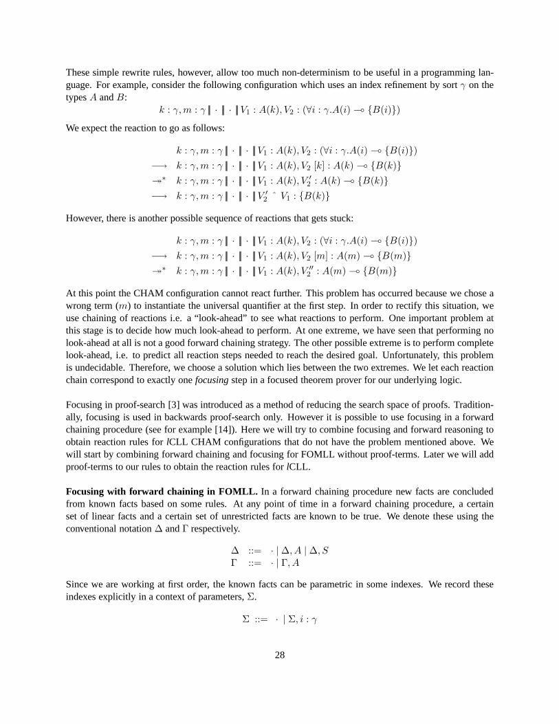
These simple rewrite rules, however, allow too much non-determinism to be useful in a programming lan-guage. For example, consider the following configuration which uses an index refinement by sortγ on thetypesA andB:

k : γ,m : γ ||| · ||| · ||| V1 : A(k), V2 : (∀i : γ.A(i) ( {B(i)})

We expect the reaction to go as follows:

k : γ,m : γ ||| · ||| · ||| V1 : A(k), V2 : (∀i : γ.A(i) ( {B(i)})

−→ k : γ,m : γ ||| · ||| · ||| V1 : A(k), V2 [k] : A(k) ( {B(k)}

�∗ k : γ,m : γ ||| · ||| · ||| V1 : A(k), V ′2 : A(k) ( {B(k)}

−→ k : γ,m : γ ||| · ||| · ||| V ′2 ˆ V1 : {B(k)}

However, there is another possible sequence of reactions that gets stuck:

k : γ,m : γ ||| · ||| · ||| V1 : A(k), V2 : (∀i : γ.A(i) ( {B(i)})

−→ k : γ,m : γ ||| · ||| · ||| V1 : A(k), V2 [m] : A(m) ( {B(m)}

�∗ k : γ,m : γ ||| · ||| · ||| V1 : A(k), V ′′2 : A(m) ( {B(m)}

At this point the CHAM configuration cannot react further. This problem has occurred because we chose awrong term (m) to instantiate the universal quantifier at the first step. Inorder to rectify this situation, weuse chaining of reactions i.e. a “look-ahead” to see what reactions to perform. One important problem atthis stage is to decide how much look-ahead to perform. At oneextreme, we have seen that performing nolook-ahead at all is not a good forward chaining strategy. The other possible extreme is to perform completelook-ahead, i.e. to predict all reaction steps needed to reach the desired goal. Unfortunately, this problemis undecidable. Therefore, we choose a solution which lies between the two extremes. We let each reactionchain correspond to exactly onefocusingstep in a focused theorem prover for our underlying logic.

Focusing in proof-search [3] was introduced as a method of reducing the search space of proofs. Tradition-ally, focusing is used in backwards proof-search only. However it is possible to use focusing in a forwardchaining procedure (see for example [14]). Here we will try to combine focusing and forward reasoning toobtain reaction rules forlCLL CHAM configurations that do not have the problem mentioned above. Wewill start by combining forward chaining and focusing for FOMLL without proof-terms. Later we will addproof-terms to our rules to obtain the reaction rules forlCLL.

Focusing with forward chaining in FOMLL. In a forward chaining procedure new facts are concludedfrom known facts based on some rules. At any point of time in a forward chaining procedure, a certainset of linear facts and a certain set of unrestricted facts are known to be true. We denote these using theconventional notation∆ andΓ respectively.

∆ ::= · | ∆, A | ∆, SΓ ::= · | Γ, A

Since we are working at first order, the known facts can be parametric in some indexes. We record theseindexes explicitly in a context of parameters,Σ.

Σ ::= · | Σ, i : γ

28

We represent the facts known at any time using the notationΣ;Γ;∆. Now the principal judgment in aforward chaining procedure is a rewrite judgmentΣ;Γ;∆ → Σ′; Γ′;∆′, which means that given the factsΣ;Γ;∆, we can conclude the factsΣ′; Γ′;∆′. In this judgment,Σ′, Γ′ and∆′ areoutputs. As it turns out,since we are dealing only with asynchronous connectives here, Σ andΓ do not change in this judgment.Thus we can write this judgment more explicitly asΣ;Γ;∆ → Σ;Γ;∆′. We have already seen someexamples of rules of this judgment(with proof-terms) earlier. We abandoned these rules because they areineffective for linking programs. The rules we saw earlier are reproduced below without proof-terms.

Σ;Γ;∆, A1&A2 → Σ;Γ;∆, A1

Σ;Γ;∆, A1&A2 → Σ;Γ;∆, A2

Σ;Γ;∆, A ( B,A → Σ;Γ;∆, BΣ;Γ, A;∆, A → B → Σ;Γ, A;∆, B

Σ ` t : γ

Σ;Γ;∆,∀i : γ.A(i) → Σ;Γ;∆, A(t)

As we saw, these rules are too general in the sense that they allow too many possible computations, all ofwhich are not desirable. Going back to our example of the computation that got stuck, we observe that wewanted to forward chain the two typesA(k) and∀i : γ.A(i) ( {B(i)} to conclude{B(k)}. This requiredinstantiation of the second type withk to obtainA(k) ( {B(k)} and then an elimination of( to obtain{B(k)}. However, using the rules presented above, we could also instantiate∀i : γ.A(i) ( {B(i)} with minstead ofk and reach a deadlock. As we noticed, we need to perform a look-ahead, or a certain amount ofreasoning to decide that we have to instantiate the second type withk, notm. This kind of look-ahead canbe done using focusing. Rather than arbitrarily selectingm or k to instantiate∀i : γ.A(i) ( {B(i)}, webegin afocuson∀i : γ.A(i) ( {B(i)}. Once this type is under a focus, we performbackwards reasoningwith backtrackingon this type to decide what to do till we have either successfully concluded a fact, or wehave exhausted all possibilities.

We present a focused forward chaining procedure for FOMLL (without proof-terms) in two steps. In thefirst step, we present some focusing rules that allow us to conclude asinglefact of the form{S} from a setof factsΣ;Γ;∆. This judgment is writtenΣ;Γ;∆ → {S}. In the second step, we modify some of theserules to obtain a focusing forward chaining procedure for FOMLL. The principal judgment of this procedureis as mentioned before -Σ;Γ;∆ → Σ;Γ;∆′.

Concluding single facts with forward chaining in FOMLL. We begin with the first step i.e. we presentfocusing rules that allow us to conclude a single fact of the form {S} from a set of factsΣ;Γ;∆. Thisprocess consumes the facts in∆. Figures 16 and 17 show four related judgments. All rules in these figuresare used backwards. The rules in figure 16 will later be replaced by a new set of rules to obtain a focusedforward chaining procedure for FOMLL.

The principal judgment in figure 16 isΣ;Γ;∆ → {S}. We read this judgment as follows - “if we candeduceΣ;Γ;∆ → {S} from the rules in figures 16 and 17 using backward reasoning, then in a forwardchaining procedure we can conclude the linear fact{S} from the unrestricted facts inΓ and the linear factsin ∆”. Thus this judgment allows us to combine forward and backward reasoning. The proposition{S} isan output of this judgment. In order to deduceΣ;Γ;∆ → {S}, we must first focus on a fact in eitherΓor ∆. This is done using one of the two rules that concludeΣ;Γ;∆ → {S}. Once we have focused ona formula, we move to the second judgment in figure 16 -Σ;Γ;∆;A ⇒ {S}. The propositionA at the

29

Contexts

Γ ::= · | Γ, A∆ ::= · | ∆, A | ∆, S

Σ;Γ;∆ → {S} (Inputs: Σ,Γ,∆; Output: {S})

Σ;Γ;∆;A ⇒ {S}→ −1

Σ;Γ;∆, A → {S}

Σ;Γ, A;∆;A ⇒ {S}→ −2

Σ;Γ, A;∆ → {S}

Σ;Γ;∆;A ⇒ {S} (Inputs: Σ,Γ,∆, A; Output: {S})

⇒ −HY P

Σ;Γ; ·; {S} ⇒ {S}Σ ` t : γ Σ;Γ;∆;A(t) ⇒ {S}

⇒ −∀

Σ;Γ;∆;∀i : γ.A(i) ⇒ {S}

Σ;Γ;∆;A1 ⇒ {S}⇒ −&1

Σ;Γ;∆;A1&A2 ⇒ {S}

Σ;Γ;∆;A2 ⇒ {S}⇒ −&2

Σ;Γ;∆;A1&A2 ⇒ {S}

Σ;Γ;∆1 →A P Σ;Γ;∆2;B ⇒ {S}⇒ − (

Σ;Γ;∆1,∆2;P ( B ⇒ {S}

Σ;Γ; · →A P Σ;Γ;∆;B ⇒ {S}⇒ − →

Σ;Γ;∆;P → B ⇒ {S}

Figure 16: Focused left rules for asynchronous connectives (Part I)

30

Σ;Γ;∆ →A P (Inputs: Σ,Γ,∆, P ; Outputs: None)

Σ;Γ;∆;A ⇒A P→A −1

Σ;Γ;∆, A →A P

Σ;Γ, A;∆;A ⇒A P→A −2

Σ;Γ, A;∆ →A P

Σ;Γ;∆;A ⇒A P (Inputs: Σ,Γ,∆, A, P ; Outputs: None)

⇒A −HY P

Σ;Γ; ·;P ⇒A PΣ ` t : γ Σ;Γ;∆;A(t) ⇒A P

⇒A −∀

Σ;Γ;∆;∀i : γ.A(i) ⇒A P

Σ;Γ;∆;A1 ⇒A P⇒A −&1

Σ;Γ;∆;A1&A2 ⇒A P

Σ;Γ;∆;A2 ⇒A P⇒A −&2

Σ;Γ;∆;A1&A2 ⇒A P

Σ;Γ;∆1 →A P ′ Σ;Γ;∆2;B ⇒A P⇒A − (

Σ;Γ;∆1,∆2;P′ ( B ⇒A P

Σ;Γ; · →A P ′ Σ;Γ;∆;B ⇒A P⇒A − →

Σ;Γ;∆;P ′ → B ⇒A P

Figure 17: Focused left rules for asynchronous connectives (Part II)

31

end of the three contexts is the formula in focus.{S} is an output in this judgment also. In this judgment,we keep eliminating the top level connective of the formula in focus till we are left with a single formulaof the form{S}. This formula{S} becomes the output of the judgment. If this does not happen, we mustbacktrack and find some other sequence of eliminations to apply.

In order to eliminate an implication (( or→), we have to show that the argument of the implication is prov-able. This requires the introduction of the auxiliary judgments shown in figure 17. They areΣ;Γ;∆ →A PandΣ;Γ;∆;A ⇒A P . The symbolA in the subscript of⇒A and→A stands forauxiliary. These judg-ments are exactly like those in figure 16 with three differences. First, the conclusion is anatomic propo-sition P instead of{S}. The proposition must be atomic because as mentioned earlier, our backwardsreasoning does not use any right rules. Second, these judgments are not principal; even if we can concludeΣ;Γ;∆ →A P , the forward chaining procedure cannot concludeP from the unrestricted factsΓ and thelinear facts∆. The judgments of figure 17 can be used only to prove that the formula needed in the argu-ment of an implication actually holds. Third, the conclusion of the sequent,P , is an input in the auxiliaryjudgments. On the other hand, the conclusion{S} is an output in the judgments of figure 16.

There are some remarks to be made here. The principal judgment Σ;Γ;∆ → {S} always has a fact ofthe type{S} in the conclusion. Thus the forward chaining procedure always concludes facts of the form{S} when it uses focusing. Further, backward search never eliminates a monad in focus. Thus the monad isalso the constructor where backwards reasoning stops. Having such a clear demarcation of where backwardreasoning stops is essential in writing correct programs.

Forward chaining rules for FOMLL. So far we have seen how we can combine focusing with forwardchaining to successfully conclude asingle fact from a number of given facts. We now come to the sec-ond step. We use the rules in figures 16 and 17 to obtain a forward chaining procedure for FOMLL. Asmentioned earlier, the principal judgment we want to obtainis Σ;Γ;∆ → Σ;Γ;∆′. This judgment isto be read as follows - “given the parametric index assumptions inΣ and the unrestricted factsΓ, we canconclude the linear facts∆′ from the linear facts∆”. We already know how to conclude a single fact froma given set of facts. Now we allow this deduction to occur in any arbitrary context. We want to say thatif Σ;Γ;∆ → {S}, then we can concludeΣ,Σ′′; Γ,Γ′′; {S},∆′′ from the factsΣ,Σ′′; Γ,Γ′′;∆,∆′′ forarbitraryΣ′′, Γ′′ and∆′′. We can integrate this closure under contexts directly intothe backwards searchrules. To do that, we reformulate the rules of figure 16. Thesemodified rules are shown in figure 18. Astep-by-step explanation of the transformation of rules isgiven below.

We begin by changing the judgmentΣ;Γ;∆ → {S} to Σ;Γ;∆ → Σ;Γ;∆′. There are two rules to derivethis new judgment, both of which are shown in figure 18. This judgment is the principal forward chainingjudgment for FOMLL and the context∆′ is an output. Next we revise the judgmentΣ;Γ;∆;A ⇒ {S}. Wechange this toΣ;Γ;∆;A ⇒ Σ;Γ;∆′. We do this one by one for all the rules. In the rule⇒ −HY P (seefigure 16), we conclude{S} if we have focused on{S}. Since we are now implementing a forward chainingrewrite judgment, we can change this to the unconditional rewrite ruleΣ;Γ;∆; {S} ⇒ Σ;Γ;∆, {S}. In therule⇒ −∀ (figure 16), we instantiate a universally quantified term in focus as we move from the conclusionof the rule to the premises and the right hand side of the sequents in the second premise and conclusion isthe same. This gives us the following revised rule:

Σ ` t : γ Σ;Γ;∆;A(t) ⇒ Σ;Γ;∆′

⇒ −∀

Σ;Γ;∆;∀i : γ.A(i) ⇒ Σ;Γ;∆′

32

Contexts

Γ ::= · | Γ, A∆ ::= · | ∆, A | ∆, S

Σ;Γ;∆ → Σ;Γ;∆′ (Inputs: Σ,Γ,∆; Output: ∆′)

Σ;Γ;∆;A ⇒ Σ;Γ;∆′→ −1

Σ;Γ;∆, A → Σ;Γ;∆′

Σ;Γ, A;∆;A ⇒ Σ;Γ;∆′→ −2

Σ;Γ, A;∆ → Σ;Γ;∆′

Σ;Γ;∆;A ⇒ Σ;Γ;∆′ (Inputs: Σ,Γ,∆, A; Output: ∆′)

⇒ −HY P

Σ;Γ;∆; {S} ⇒ Σ;Γ;∆, {S}Σ ` t : γ Σ;Γ;∆;A(t) ⇒ Σ;Γ;∆′

⇒ −∀

Σ;Γ;∆;∀i : γ.A(i) ⇒ Σ;Γ;∆′

Σ;Γ;∆;A1 ⇒ Σ;Γ;∆′⇒ −&1

Σ;Γ;∆;A1&A2 ⇒ Σ;Γ;∆′

Σ;Γ;∆;A2 ⇒ Σ;Γ;∆′⇒ −&2

Σ;Γ;∆;A1&A2 ⇒ Σ;Γ;∆′

Σ;Γ;∆1 →A P Σ;Γ;∆2;B ⇒ Σ;Γ;∆′⇒ − (

Σ;Γ;∆1,∆2;P ( B ⇒ Σ;Γ;∆′

Σ;Γ; · →A P Σ;Γ;∆;B ⇒ Σ;Γ;∆′⇒ − →

Σ;Γ;∆;P → B ⇒ Σ;Γ;∆′

Figure 18: Judgments→ and⇒ for forward chaining in FOMLL

The rules⇒ −&1 and⇒ −&2 can be modified similarly (see figure 18). For the rules⇒ − ( and⇒ − →, we need to replace the{S} in the right hand sides of the sequents byΣ;Γ;∆′. In this manner wecan revise the entire system in figure 16 and obtain the systemin figure 18. The judgments→A and⇒A infigure 17 are auxiliary and do not change.

In summary, the rules of figures 17 and 18 are focused rewrite rules for a forward chaining procedure forFOMLL. The principal judgment isΣ;Γ;∆ → Σ;Γ;∆′ (figure 18). It is used as follows. If using backwardreasoning we can conclude the judgmentΣ;Γ;∆ → Σ;Γ;∆′, then in a forward chaining procedure forFOMLL, we can conclude the linear facts∆′ from the linear facts∆, if the unrestricted context has the thefactsΓ. Further, this conclusion is parametric in the assumptionsin Σ. As remarked earlier, the backwardsearch procedure constructs the set of facts∆′. We now augment these rules with proof-terms to obtainreaction rules for CHAM configurations.

Reaction rules for CHAMs. We augment the rules in figures 18 and 17 with proof-terms to obtain focused

33

reaction rules forlCLL-CHAMs. These new rules are shown in figures 19 and 20. The judgments−→, =⇒,−→A and=⇒A are obtained by adding proof-terms to the judgments→, ⇒, →A and⇒A respectively. Wealso add the context of substitutionsσ to all our judgments. This process is straightforward. As anillus-tration, we explain some of the rules. In the rule=⇒ −&1, we have a focus on a formulaA1&A2, whoseproof-term isN . As we reason backwards, we replaceA1&A2 byA1 and its witnessN by π1 N , which is aproof ofA1. In the rule=⇒ −∀, we instantiate the proofN of ∀i : γ.A(i) by a concrete index term. Sincewe assumed earlier that index variables in the domain ofσ must not occur in terms inside configurations, weinstantiateN with t[σ] instead oft.4 Observe thatN [t[σ]] has the typeA(t)[σ] if N has the type∀i : γ.A(i)andt : γ. The rule−→ −{} is a new rule to eliminate the monadic constructor, as mentioned earlier. It isinstructive to compare figures 18 and 17 with figures 19 and 20 respectively.

As for the case of FOMLL, these rules are conditional rewriterules for CHAM configurations that usebackward reasoning and focusing. The principal judgment here is Σ ||| σ ||| Γ ||| ∆ −→ Σ ||| σ ||| Γ ||| ∆′. Theinterpretation is the same as before - if we can conclude the judgmentΣ ||| σ ||| Γ ||| ∆ −→ Σ ||| σ ||| Γ ||| ∆′ usingbackward reasoning, then the CHAM configurationΣ ||| σ ||| Γ ||| ∆ rewrites to the configurationΣ ||| σ ||| Γ ||| ∆′

using a single reaction step.

The typeP in the judgmentΣ ||| σ ||| Γ ||| ∆ =⇒A N : P must be atomic because we do not use right rulesfor asynchronous connectives in our proof-search. One consequence of this is that all arguments passed tofunctions during the focusing steps have atomic types i.e. in the rules=⇒ − ( and=⇒ − →, the termN1

is forced to have an atomic typeP (see figure 19). In order to pass values of other types to functions duringthe linking steps, the values must be abstracted to atomic types. This requires an extension of the languagewith suitable primitives like datatypes as in ML.5

This completes our discussion of rewrite rules forlCLL CHAMs. In summary, there are three types ofrewrite rules inlCLL: structural (⇀), functional (�) and reaction (−→). Structural and functional rules areshown in figure 14. Reaction rules require some backward reasoning. They are shown in figures 19 and 20.

3.2 Programming Technique: Creating Private Names

We illustrate here how to use the existential quantifier to create fresh names. Suppose we have aconstantcγ : γ in the sortγ. Now consider a typed monadic term of the form[cγ ,M(cγ)] # ∃i : γ.S(i). If this termis put in a solution, the only way it rewrites is using the rule⇀ −∃:

Σ ||| σ ||| Γ ||| ∆, [cγ ,M(cγ)] # ∃i : γ.S(i) ⇀ Σ, k : γ ||| σ, cγ/k : γ ||| Γ ||| ∆,M(cγ) # S(k)

In the typeS(i) on the right hand side,cγ has been abstracted byk which is a fresh name by the sidecondition on this rewrite rule. In effect, we have created a fresh namek of sortγ. We can use this mechanismto create more private names using the same namecγ for the index term again and again. Based on this idea,we define a new language construct as follows.

priv k : γ in M # S(k) =[cγ , M [cγ/k] ] # ∃i : γ.S(i)

4Since this rule is used backward,t is determined through unification in a practical implementation. Thus in practice this rule isimplemented as follows. We replacei with a unification variableX to obtain the typeA(X). Unification on types determines theexact index termt that substitutesX. Then we instantiateN with t[σ].

5Datatypes can also be implemented by introducing existential, recursive and sum types at the level of pure terms.

34

Σ ||| σ ||| Γ ||| ∆ −→ Σ ||| σ ||| Γ ||| ∆′ (Inputs: Σ, σ, Γ, ∆; Output: ∆′)

Σ ||| σ ||| Γ ||| ∆ ||| V : A =⇒ Σ ||| σ ||| Γ ||| ∆′

−→ − =⇒ −1

Σ ||| σ ||| Γ ||| ∆, V : A −→ Σ ||| σ ||| Γ ||| ∆′

Σ ||| σ ||| Γ, V : A ||| ∆ ||| V : A =⇒ Σ ||| σ ||| Γ, V : A ||| ∆′

−→ − =⇒ −2

Σ ||| σ ||| Γ, V : A ||| ∆ −→ Σ ||| σ ||| Γ, V : A ||| ∆′

−→ −{}

Σ ||| σ ||| Γ ||| ∆, {E} : {S} −→ Σ ||| σ ||| Γ ||| ∆, E ÷ S

Σ ||| σ ||| Γ ||| ∆ ||| N : A =⇒ Σ ||| σ ||| Γ ||| ∆′ (Inputs: Σ, σ, Γ, ∆,N,A; Output: ∆′)

=⇒ −HY P

Σ ||| σ ||| Γ ||| ∆ ||| N : {S} =⇒ Σ ||| σ ||| Γ ||| ∆,N : {S}

Σ ` t : γ Σ ||| σ ||| Γ ||| ∆ ||| N [t[σ]] : A(t) =⇒ Σ ||| σ ||| Γ ||| ∆′

=⇒ −∀

Σ ||| σ ||| Γ ||| ∆ ||| N : ∀i : γ.A(i) =⇒ Σ ||| σ ||| Γ ||| ∆′

Σ ||| σ ||| Γ ||| ∆ ||| π1 N : A1 =⇒ Σ ||| σ ||| Γ ||| ∆′

=⇒ −&1

Σ ||| σ ||| Γ ||| ∆ ||| N : A1&A2 =⇒ Σ ||| σ ||| Γ ||| ∆′

Σ ||| σ ||| Γ ||| ∆ ||| π2 N : A2 =⇒ Σ ||| σ ||| Γ ||| ∆′

=⇒ −&2

Σ ||| σ ||| Γ ||| ∆ ||| N : A1&A2 =⇒ Σ ||| σ ||| Γ ||| ∆′

Σ ||| σ ||| Γ ||| ∆1 −→A N1 : P Σ ||| σ ||| Γ ||| ∆2 ||| N2 ˆN1 : A =⇒ Σ ||| σ ||| Γ ||| ∆′

=⇒ − (

Σ ||| σ ||| Γ ||| ∆1, ∆2 ||| N2 : P ( A =⇒ Σ ||| σ ||| Γ ||| ∆′

Σ ||| σ ||| Γ ||| · −→A N1 : P Σ ||| σ ||| Γ ||| ∆ ||| N2 N1 : A =⇒ Σ ||| σ ||| Γ ||| ∆′

=⇒ − →

Σ ||| σ ||| Γ ||| ∆ ||| N2 : P → A =⇒ Σ ||| σ ||| Γ ||| ∆′

Figure 19: Reaction rules for the CHAM (Part I)

35

Σ ||| σ ||| Γ ||| ∆ −→A N : P (Inputs: Σ, σ, Γ, ∆, P ; Output: N )

Σ ||| σ ||| Γ ||| ∆ ||| V : A =⇒A N : P−→A − =⇒A −1

Σ ||| σ ||| Γ ||| ∆, V : A −→A N : P

Σ ||| σ ||| Γ, V : A ||| ∆ ||| V : A =⇒A N : P−→A − =⇒A −2

Σ ||| σ ||| Γ, V : A ||| ∆ −→A N : P

Σ ||| σ ||| Γ ||| ∆ ||| N′ : A =⇒A N : P (Inputs: Σ, σ, Γ, ∆,N ′, A, P ; Output: N )

=⇒A −HY P

Σ ||| σ ||| Γ ||| · ||| N : P =⇒A N : P

Σ ` t : γ Σ ||| σ ||| Γ ||| ∆ ||| N ′ [t[σ]] : A(t) =⇒A N : P=⇒A −∀

Σ ||| σ ||| Γ ||| ∆ ||| N ′ : ∀i : γ.A(i) =⇒A N : P

Σ ||| σ ||| Γ ||| ∆ ||| π1 N′ : A1 =⇒A N : P

=⇒A −&1

Σ ||| σ ||| Γ ||| ∆ ||| N ′ : A1&A2 =⇒A N : P

Σ ||| σ ||| Γ ||| ∆ ||| π2 N′ : A2 =⇒A N : P

=⇒A −&2

Σ ||| σ ||| Γ ||| ∆ ||| N ′ : A1&A2 =⇒A N : P

Σ ||| σ ||| Γ ||| ∆1 −→A N1 : P Σ ||| σ ||| Γ ||| ∆2 ||| N2 ˆN1 : A =⇒A N : P ′

=⇒A − (

Σ ||| σ ||| Γ ||| ∆1, ∆2 ||| N2 : P ( A =⇒A N : P ′

Σ ||| σ ||| Γ ||| · −→A N1 : P Σ ||| σ ||| Γ ||| ∆ |||N2 N1 : A =⇒A N : P ′

=⇒A − →

Σ ||| σ ||| Γ ||| ∆ ||| N2 : P → A =⇒A N : P ′

Figure 20: Reaction rules for the CHAM (Part II)

36

Syntax

A ::= x〈y1 . . . yn〉 | x(y1 . . . yn).P (Actions)C ::= A | C + C (External Choice)P ::= C | P |P | νx.P | 0 (Processes)

CHAM solutions

m ::= P | νx.S (Molecules)S ::= φ | S ] {m} (Solutions)

Equations on terms and solutions

C1 + (C2 + C3) = (C1 + C2) + C3

C1 + C2 = C2 + C1

νx.P = νy.P [y/x] y 6∈ Pνx.S = νy.S[y/x] y 6∈ S

CHAM semantics

x(y1 . . . yn).P + C1 , xz1 . . . zn + C2 → P [z1/y1] . . . [zn/yn]νx.P ⇀ νx.{P}

νx.S, P ⇀ νx.(S ] {P})P1|P2 ⇀ P1, P2

0 ⇀

Figure 21: Theπ-calculus: syntax and semantics

The typing rule for this construct is

Σ, k : γ; Γ;∆;Ψ ` M # S(k)priv

Σ;Γ;∆;Ψ ` (priv k : γ inM # S(k)) # ∃i : γ.S(i)

3.3 Example: Encoding theπ-calculus

In this section, we show an encoding of variant of theπ-calculus [6] inlCLL. The syntax and semanticsof theπ-calculus we use are shown in figure 21. The encoding we choosefor this calculus is based on anencoding of a similar calculus in MSR [11]. We assume that thesignature for our language contains a familyof type constructorsoutn for n = 0, 1, . . .. These have the kinds:

out0 : chan → Type

out1 : chan → chan → Type

out2 : chan → chan → chan → Type...

37

Assume also that we have a family of constantsout0, out1, . . . having the types:

out0 : ∀x : chan. out0 xout1 : ∀x : chan. ∀y1 : chan. out1 x y1

out2 : ∀x : chan. ∀y1 : chan. ∀y2 : chan. out2 x y1 y2...

In effect, for any n, and anyk1, . . . , kn+1 : chan, outn k1 . . . kn+1 is actually asingleton typei.e. theonly closed value of this type isoutn [k1] . . . [kn+1]. Let us also assume a family of destructor functionsdestroyout

nwhich have the types:

destroyout0

: ∀x : chan. out0 x ( {1}

destroyout1

: ∀x : chan. ∀y1 : chan. out1 x y1 ( {1}

destroyout2

: ∀x : chan. ∀y1 : chan. ∀y2 : chan. out2 x y1 y2 ( {1}...

The corresponding reduction rule is:

destroyoutn

[k1] . . . [kn+1] ˆ (outn [k1] . . . [kn+1]) → {1}

We now translate theπ-calculus into our language. Everyπ-calculus term is translated into a type and aterm. These translations are shown in figure 22. Letfn(A), fn(C) andfn(P ) stand for the free namescontained in an action, choice and process respectively. Then the following typing lemma holds.

Lemma 10 (Typing of translated terms).

1. fn(A) : chan; ·; ·; · ` pAq : ppAqq

2. fn(C) : chan; ·; ·; · ` pCq : ppCqq

3. fn(P ) : chan; ·; ·; · ` pPq # ppPqq

Proof. By induction on the structure of theπ-calculus termA, C or P .

Definition 3 (Translation of π-terms). We define the translation,〈P 〉 of aπ-termP as the CHAM config-urationfn(P ) : chan ||| · ||| · ||| pPq # ppPqq.

To illustrate how reductions occur in this framework, consider theπ-process,P = (x〈y〉+C1) | (x(z).0+C2). The translation of this process at types and terms is:

ppPqq = (out1 x y & ppC1qq) ⊗ ((∀z : chan. out1 x z ( {1}) & ppC2qq)pPq = 〈out1 [x] [y], pC1q〉 ⊗ 〈N1(x), pC2q〉

whereN1(x) is an abbreviation defined as follows:

N1(x) = Λz : chan. λm : out1 x z.{let {1} = destroyout

1[x] [z] ˆm

in 1}

38

Translation into types

ppx〈y1, . . . yn〉qq = outn x y1 . . . yn

ppx(y1, . . . , yn).Pqq = ∀y1 . . . yn : chan. outn x y1 . . . yn ( {ppPqq}ppC1 + C2qq = ppC1qq & ppC2qq

pp0qq = 1ppP1|P2qq = ppP1qq ⊗ ppP2qq

ppνx.Pqq = ∃x : chan.ppPqq

Translation into terms

px〈y1, . . . yn〉q = outn [x] [y1] . . . [yn]

px(y1, . . . , yn).Pq = Λy1 . . . yn : chan. λm : outn x y1 . . . yn.{let {1} = destroyout

n[x] [y1] . . . [yn] ˆm

in

pPq

}pC1 + C2q = 〈pC1q, pC2q〉p0q = 1pP1|P2q = pP1q ⊗ pP2q

pνx.Pq = priv x : chan in pPq

Figure 22: Translation of theπ-calculus

39

The processP reduces to0 in theπ-calculus. Correspondingly we have the following reduction sequenceon the translated term:

〈P 〉 = x : chan, y : chan ||| · ||| · ||| pPq # ppPqq

⇀ x : chan, y : chan ||| · ||| · ||| 〈out1 [x] [y], pC1q〉 # (out1 x y & ppC1qq),〈N1(x), pC2q〉 # ((∀z : chan. out1 x z ( {1}) & ppC2qq)

⇀2 x : chan, y : chan ||| · ||| · ||| 〈out1 [x] [y], pC1q〉 : (out1 x y & ppC1qq),〈N1(x), pC2q〉 : ((∀z : chan. out1 x z ( {1}) & ppC2qq)

−→ x : chan, y : chan ||| · ||| · ||| (π1 〈N1(x), pC2q〉) [y] ˆ (π1 〈out1 [x] [y], pC1q〉) : {1} (1)�∗ x : chan, y : chan ||| · ||| · ||| {let {1} = destroyout

1[x] [y] ˆ (out1 [x] [y]) in 1} : {1}

−→ x : chan, y : chan ||| · ||| · ||| (let {1} = destroyout1

[x] [y] ˆ (out1 [x] [y]) in 1) ÷ 1 (2)

� x : chan, y : chan ||| · ||| · ||| (let {1} = {1} in 1) ÷ 1� x : chan, y : chan ||| · ||| · ||| 1 ÷ 1⇀ x : chan, y : chan ||| · ||| · ||| 1 # 1⇀ x : chan, y : chan ||| · ||| · ||| ·

The reactionsteps here have been marked(1) and(2). Step(2) is the elimination of{. . .} in the monad.Step(1) requires some backwards reasoning and the exact proof that allows this step is shown in figure 23.All rules used in this proof are from figure 19. It is instructive to observe that chaining of reactions allowsus to simulate the correct behavior of external choice in theπ-calculus. The remaining steps in the abovereduction are either structural rearrangement (⇀) or functional evaluation (�).

The rewrite steps shown above show howπ-calculus reductions are simulated in the translation. Theexactformulation of a correctness result for the translation requires a notion of observation onlCLL-CHAMconfigurations, which is a subject of future research.

3.4 Types forlCLL CHAM Configurations

Since terms inlCLL CHAM configurations already have types with them, we needto create a judgmentlike Σ;Γ;∆;Ψ ` Σ′ ||| σ ||| Γ ||| ∆ in order to typelCLL CHAM configurations. The obvious intu-ition of splitting resources in∆ for all terms in∆ does not not work. For example, consider proving·; ·; ·;∆ ` · ||| · ||| · ||| x1 : A1, x2 : A2 when∆ = x1 ⊗x2 : A1 ⊗A2. Intuitively, we want this to be provablebut∆ is a singleton and cannot be split. From such observations, we arrive at the following definition.

Definition 4 (lCLL typing relation). LetΣ′ ||| σ ||| Γ ||| ∆ be a CHAM configuration. Let∆ = T1 %Z1 . . . Tn %Zn

andΓ = V1 : A1 . . . Vm : Am. We say thatΣ;Γ;∆;Ψ ` Σ′ ||| σ ||| Γ ||| ∆ iff there exist∆1 . . .∆n, Γ′ andΣ′′

such that the following conditions hold:

1. Σ′′ ⊇ Σ′

2. Σ′′; Γ′;∆1 . . .∆n ⇐= Σ;Γ;∆

3. For eacht/i : γ ∈ σ, i : γ ∈ Σ′ andΣ′′ ` t : γ

4. For1 ≤ i ≤ n, Σ′′; Γ′;∆i; Ψ ` Ti % Zi[σ]

5. For1 ≤ j ≤ m, Σ′′; Γ′; ·; Ψ ` Vj : Aj [σ]

40

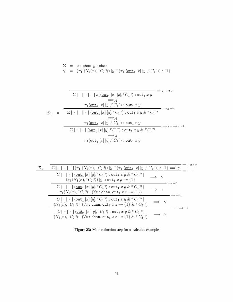
Σ = x : chan, y : chanγ = (π1 〈N1(x), pC2q〉) [y] ˆ (π1 〈out1 [x] [y], pC1q〉) : {1}

D1 =

=⇒A −HY P

Σ ||| · ||| · ||| · ||| π1〈out1 [x] [y], pC1q〉 : out1 x y=⇒A

π1〈out1 [x] [y], pC1q〉 : out1 x y=⇒A −&1

Σ ||| · ||| · ||| · ||| 〈out1 [x] [y], pC1q〉 : out1 x y & ppC1qq

=⇒A

π1〈out1 [x] [y], pC1q〉 : out1 x y−→A − =⇒A −1

Σ ||| · ||| · ||| 〈out1 [x] [y], pC1q〉 : out1 x y & ppC1qq

−→A

π1〈out1 [x] [y], pC1q〉 : out1 x y

D1

=⇒ −HY P

Σ ||| · ||| · ||| · ||| (π1 〈N1(x), pC2q〉) [y] ˆ (π1 〈out1 [x] [y], pC1q〉) : {1} =⇒ γ=⇒ − (

Σ ||| · ||| · ||| 〈out1 [x] [y], pC1q〉 : out1 x y & ppC1qq |||(π1〈N1(x), pC2q〉) [y] : out1 x y ( {1}

=⇒ γ

=⇒ −∀

Σ ||| · ||| · ||| 〈out1 [x] [y], pC1q〉 : out1 x y & ppC1qq |||π1〈N1(x), pC2q〉 : (∀z : chan. out1 x z ( {1})

=⇒ γ

=⇒ −&1

Σ ||| · ||| · ||| 〈out1 [x] [y], pC1q〉 : out1 x y & ppC1qq |||〈N1(x), pC2q〉 : (∀z : chan. out1 x z ( {1} & ppC2qq)

=⇒ γ

−→ − =⇒ −1

Σ ||| · ||| · ||| 〈out1 [x] [y], pC1q〉 : out1 x y & ppC1qq,〈N1(x), pC2q〉 : (∀z : chan. out1 x z ( {1} & ppC2qq)

−→ γ

Figure 23: Main reduction step forπ-calculus example

41

We also say thatΣ;Γ;∆;Ψ ` Σ′ ||| σ ||| Γ ||| ∆ ||| N : A iff Σ;Γ;∆;Ψ ` Σ′ ||| σ ||| Γ ||| ∆,N : A.

This definition essentially allows the context∆ to be split into several contexts, one for each of the terms in∆.

Lemma 11. Let Σ′ ||| σ ||| Γ ||| ∆ be a CHAM configuration. Let∆ = T1 % Z1 . . . Tn % Zn, Γ = V1 :A1 . . . Vm : Am and suppose there exist∆, ∆1 . . .∆n, Γ, Σ andΨ such that the following hold:

1. Σ ⊇ Σ′.

2. For eacht/i : γ ∈ σ, i : γ ∈ Σ′ andΣ ` t : γ

3. For each1 ≤ i ≤ n, Σ;Γ;∆i; Ψ ` Ti % Zi[σ]

4. For each1 ≤ j ≤ m, Σ;Γ; ·; Ψ ` Vj : Aj [σ]

5. Σ;Γ;∆;Ψ ` N : A[σ]

Then,

1. Σ;Γ;∆1 . . .∆n; Ψ ` Σ′ ||| σ ||| Γ ||| ∆.

2. Σ;Γ;∆,∆1 . . .∆n; Ψ ` Σ′ ||| σ ||| Γ ||| ∆ ||| N : A.

3. If Σ′ ||| σ ||| Γ ||| ∆ ||| N : A =⇒A N ′ : P , thenΣ;Γ;∆,∆1 . . .∆n; Ψ ` N ′ : P [σ].

4. If Σ′ ||| σ ||| Γ ||| ∆ −→A N ′ : P , thenΣ;Γ;∆1 . . .∆n; Ψ ` N ′ : P [σ].

Proof. Proof of (1) and (2) is immediate from definition 4. Proof of (3) and (4) follows by a mutual induc-tion on the given rewrite derivation.

Lemma 12.

1. If Σ;Γ;∆;Ψ ` Σ ||| σ ||| Γ ||| ∆ and Σ ||| σ ||| Γ ||| ∆ ⇀ Σ′ ||| σ′ ||| Γ′ ||| ∆′, then Σ ⊆ Σ′ andΣ′; Γ;∆;Ψ ` Σ′ ||| σ′ ||| Γ′ ||| ∆′.

2. If Σ;Γ;∆;Ψ ` Σ ||| σ ||| Γ ||| ∆ andΣ ||| σ ||| Γ ||| ∆ � Σ ||| σ ||| Γ ||| ∆′, thenΣ;Γ;∆;Ψ ` Σ ||| σ ||| Γ ||| ∆′.

3. If Σ;Γ;∆;Ψ ` Σ ||| σ ||| Γ ||| ∆ |||N ′ : A andΣ ||| σ ||| Γ ||| ∆ |||N ′ : A =⇒A N : P , thenΣ;Γ;∆;Ψ ` N :P [σ].

4. If Σ;Γ;∆;Ψ ` Σ ||| σ ||| Γ ||| ∆ andΣ ||| σ ||| Γ ||| ∆ −→A N : P , thenΣ;Γ;∆;Ψ ` N : P [σ].

5. If Σ;Γ;∆;Ψ ` Σ ||| σ ||| Γ ||| ∆ ||| N : A and Σ ||| σ ||| Γ ||| ∆ ||| N : A =⇒ Σ ||| σ ||| Γ ||| ∆′, thenΣ;Γ;∆;Ψ ` Σ ||| σ ||| Γ ||| ∆′.

6. If Σ;Γ;∆;Ψ ` Σ ||| σ ||| Γ ||| ∆ andΣ ||| σ ||| Γ ||| ∆ −→ Σ ||| σ ||| Γ ||| ∆′, thenΣ;Γ;∆;Ψ ` Σ ||| σ ||| Γ ||| ∆′.

Proof. Proof of (1) follows from lemma 5. (2) is immediate from lemma8. (3) and (4) follow from lemma11 and lemma 1(3). For (5) we use induction on the derivation of the given rewrite relation and lemma 11.(6) follows immediately from (5).

42

Definition 5 (lCLL CHAM moves). We define alCLL CHAM rewrite move⇒ as⇒ = ⇀ ∪ � ∪ −→.⇒∗ denotes the reflexive-transitive closure of⇒.

Lemma 13 (lCLL preservation). If Σ;Γ;∆;Ψ ` Σ ||| σ ||| Γ ||| ∆ andΣ ||| σ ||| Γ ||| ∆ ⇒∗ Σ′ ||| σ′ ||| Γ′ ||| ∆′, thenΣ ⊆ Σ′ andΣ′; Γ;∆;Ψ ` Σ′ ||| σ′ ||| Γ′ ||| ∆′.

Theorem 2 (Type-safety for terms inlCLL CHAMs). If Σ; ·; ·; · ` Σ ||| σ ||| Γ ||| ∆ andΣ ||| σ ||| Γ ||| ∆ ⇒∗

Σ′ ||| σ′ ||| Γ′ ||| ∆′, then for any typedf CLL termT % Z in ∆′, it is the case thatT is a value orT reduces tosomeT ′.

Proof. Using lemma 13,Σ′; ·; ·; · ` Σ′ ||| σ′ ||| Γ′ ||| ∆′. Let ∆′ = T1 % Z1, . . . , Tn % Zn. By defini-tion 4, there existΣ′′,Γ′,∆1, . . . ,∆n such thatΣ′′; Γ′;∆1, . . . ,∆n ⇐= Σ′; ·; · and for each1 ≤ i ≤ n,Σ′′; Γ′;∆i; · ` Ti % Zi[σ

′]. Now from lemma 1 it is clear thatΓ′ = · and∆1 = . . . = ∆n = ·. Thus, foreach1 ≤ i ≤ n, Σ′′; ·; ·; · ` Ti % Zi[σ

′]. Using the progress lemma forf CLL (lemma 9), eachTi musteither be a value, or it can reduce further.

3.5 Comparing process-calculi andlCLL

As seen from the encoding of theπ-calculus in section 3.3,lCLL can encode several basic concurrencyprimitives. In fact, there is a correspondence between the constructs of process-calculi like theπ-calculusand constructors oflCLL. Various common constructs of process-calculi, together with their equivalents inlCLL are listed below.

1. Processes. In general, we view monadic terms and expressions as processes in CHAM solutions.

2. Parallelism. Apart from parallelism introduced for expressions in section 2.1, monadic terms of theformM1 ⊗M2 can be viewed as processes reducing in parallel. Similarly,terms in CHAM solutionscan be viewed as processes executing in parallel.

3. Communication channels.Communication channels can be simulated inlCLL using index refine-ments of a fixed sort (chan ) as we do in section 3.3.

4. Input prefixing. The language constructsΛi.N , λx : P.N andλx : P.N together with the associatedtypes∀i : γ.A, P → B andP ( B provide encodings for input processes.

5. Asynchronous output. Any valueV of (possibly refined) atomic typeP can be viewed as an outputterm without continuation because it can be linked to a term of type P ( B as an input. If thevalueV : P is linear, then this corresponds to an output that has to be used as an input to exactly oneprogram. If it is unrestricted, then it can be used as input toany number of programs. Such an outputterm corresponds to an asynchronous broadcast.

6. Name restriction. We showed in section 3.2 that channels can be made private using abstractionsemantics of the∃ quantifier. Thepriv construct defined in that section can be used to create privatechannel names in CHAM executions.

7. Choices. The type constructor& and the associated term constructor〈N1,N2〉 act as an externalchoice operator in our logic programming language. The proof-search procedure can project out onecomponent of a choice if it can be used to complete a link step.The type constructor⊕ and themonadic term constructorsinl andinr can be used to simulate internal choice inlCLL.

43

Process-calculus construct EquivalentlCLL constructProcess,P Monadic term(M ), expression(E)Parallel composition,P1|P2 M1 ⊗M2 # S1 ⊗ S2

Communication channel Index refinement of sortchanInput prefixing,x(y).P Λi.N : ∀i : γ.A, λx.N : P → B andλx.N : P ( BAsynchronous output,xy Linear assumptionN : P whereP is atomicName restriction,νx.P priv x : chan inM # ∃x : chan.SInternal choice inlM # S1 ⊕ S2, inrM # S1 ⊕ S2

External choice,C1 + C2 〈N1,N2〉 : A1&A2

n-way input N : P1 ( . . . ( Pn ( BCommunication and synchronizationProof-search

Figure 24: Correspondence between process-calculi andlCLL

8. n-way input. Due to chaining of linking steps in thelCLL, we have a mechanism for n-way input inlCLL. For example, a receiver of typeP1 ( P2 ( B alwayssynchronizes simultaneously with twosenders of typesP1 andP2.

9. Communication and synchronization. Communication and synchronization inlCLL occurs usingreaction steps (−→).

For an illustration of these constructs inlCLL, the reader is referred to the encoding of theπ-calculus insection 3.3. Figure 24 shows a summary of the above correspondence between process-calculi constructsandlCLL connectives.

4 Full-CLL: Integrating fCLL and lCLL

f CLL described in section 2 is purely functional. Even thoughit admits some parallelism in the tensor andevaluation of expressions, it is essentially free from effects. The concurrent (logic) programming languagelCLL described in section 3 allows an additional layer of concurrency overf CLL. In this section we integratein the other direction - we allow concurrent logic programming to occur insidef CLL programs. Sinceconcurrent computations can deadlock and get stuck, they are not free from effects. As a result, we confinesuch concurrent evaluation to the monad only. We extend the grammar for expressions with an additionalconstruct as follows.

E ::= . . . | link (E ÷ S) to G

whereG ::= A | !A | 1 andA is any asynchronous type.G is called a goal type. Observe thatG is a subsetof the family of types. We do not allow arbitrary types as goals for reasons described later. The typing rulefor thelink construct is the following.

Σ;Γ;∆;Ψ ` E ÷ SLINK

Σ;Γ;∆;Ψ ` link (E ÷ S) to G ÷ G

It is assumed in the above rule thatG is well-formed in the contextΣ. The link construct is alwaysevaluated in the context of index variablesΣ in which it is well-typed. To evaluateΣ; link (E ÷ S) to G

44

we start a newlCLLCHAM configuration with only the termE ÷ S in it i.e. we start withΣ ||| · ||| · |||E ÷ S.Then we let this configuration rewrite according to all the rules in figures 14, 19 and 20until it saturatesi.e. no more rewrite rules apply. If the configuration never saturates, computation runs forever and thelink

construct does not terminate. If the configuration saturates inΣ′ ||| σ ||| Γ ||| ∆, then the computation of thelinkconstruct succeeds iff one of the following conditions holds.

1. G = A and∆ = V : A. Then the whole construct evaluates toΣ′;V .

2. G = A, ∆ = · and there existsV : A ∈ Γ. In this case the whole construct evaluates toΣ′;V .

3. G =!A, ∆ = · and there existsV : A ∈ Γ. Then the whole construct evaluates toΣ′; !V .

4. G = 1 and∆ = ·. In this case the whole construct evaluates toΣ′; 1.

If none of these conditions hold, then the computation failsand evaluation deadlocks. The above conditionsare summarized in the following evaluation rules.

Σ ||| · ||| · ||| E ÷ S ⇒∗ Σ′ ||| σ ||| Γ ||| V : A↪→ LINK − 1

Σ; link (E ÷ S) to A ↪→ Σ′;V

Σ ||| · ||| · ||| E ÷ S ⇒∗ Σ′ ||| σ ||| Γ, V : A ||| ·↪→ LINK − 2

Σ; link (E ÷ S) to A ↪→ Σ′;V

Σ ||| · ||| · ||| E ÷ S ⇒∗ Σ′ ||| σ ||| Γ, V : A ||| ·↪→ LINK − 3

Σ; link (E ÷ S) to !A ↪→ Σ′; !V

Σ ||| · ||| · ||| E ÷ S ⇒∗ Σ′ ||| σ ||| Γ ||| ·↪→ LINK − 4

Σ; link (E ÷ S) to 1 ↪→ Σ′; 1

where⇒ = ⇀ ∪ � ∪ −→, as in definition 5. It is implicitly assumed in these rules that any CHAMconfiguration on the right of⇒∗ is saturated (it cannot be rewritten using the relation⇒). We also lift theevaluation relationE ↪→ E′ from figure 12 to include the contextΣ.

E ↪→ E′

Σ;E ↪→ Σ;E′

At this point we can explain why we restrict the goalG in the constructlink (E ÷ S) to G to the set{A, !A, 1}. The reason for disallowing arbitrary goals is that for goaltypes other than{A, !A, 1}, compu-tation of thelink construct will always fail because saturated CHAM configurations cannot contain termshaving those types. Suppose, for example, we allow the typeG = S1 ⊗S2 as a goal. In order for evaluationto succeed withS1 ⊗ S2 as a goal, the CHAM rewriting would have to end in a configuration Σ′ ||| σ ||| Γ ||| ∆where∆ = M # S1 ⊗ S2, for someM . However, this is impossible because at this point the CHAM con-figuration cannot be saturated. We can prove this as follows.By the progress theorem, eitherM is a value,or it can reduce further. IfM is a value, it has to be of the formMv1

⊗Mv2and in that case we can apply the

rule⇀ −⊗ on the CHAM configuration. IfM can reduce further, then the whole CHAM configuration canreduce using the rule� − 7→. Thus anlCLL CHAM configuration cannot end with a monadic term of typeS1⊗S2 in ∆. Similar arguments show that a CHAM configuration cannot saturate if it has a program ofanysynchronous type in it. For the particular set of goals,{A, !A, 1}, it is possible for CHAM computations tosucceed without any synchronous types in them. Thus we limitgoals to this set. Limiting goal types to the

45

set{A, !A, 1} may seem like a big restriction but in practice we found that other goal types are never needed.

We call the resultant language with thelink construct full-CLL or CLL for brevity. Full-CLL symmetri-cally integrates functional and concurrent logic programming. Concurrent logic programming can be nestedinsidef CLL programs using thelink construct. On the other hand, the functional rewrite rules in CHAMsallow functional evaluation inside concurrent logic programming. Execution of full-CLL programs occursin interleaving phases of functional evaluation and concurrent logic programming.

An important remark related to programming in full-CLL is that it is essential that the top-level constructof any program that performs concurrent computation be an expression. This is because all concurrency infull-CLL is restricted to thelink construct which is an expression, and evaluation of expressions coercedinto terms is lazy (recall that{E} is a value in CLL). If the top-level construct of a program is aterm or amonadic term, then nested expressions in the program will never be evaluated, and hence the program willnot perform any concurrent computation.

4.1 Type-Safety

Since thelink construct may get stuck, full-CLL does not have a progress lemma at the level of expres-sions. However the monad in CLL is lazy and this lemma still holds at the level of terms and monadic terms.We also have a type preservation lemma at the level of terms, monadic terms and expressions. Type-safetylemmas and theorems for full-CLL are given below.

Lemma 14 (Preservation).

1. If Σ;Γ;∆;Ψ ` N : A andN → N ′, thenΣ;Γ;∆;Ψ ` N ′ : A.

2. If Σ;Γ;∆;Ψ ` M # S andM 7→ M ′, thenΣ;Γ;∆;Ψ ` M ′ # S.

3. If Σ;Γ;∆;Ψ ` E ÷ S andΣ;E ↪→ Σ′;E′, thenΣ ⊆ Σ′ andΣ′; Γ;∆;Ψ ` E′ ÷ S.

Proof. In this case we use induction on the given derivation to simultaneously prove this and lemmas 12and 13.

Lemma 15 (Progress).

1. If Σ; ·; ·; · ` N : A, then eitherN = V or for someN ′,N → N ′.

2. If Σ; ·; ·; · ` M # S, then eitherM = Mv or for someM ′,M 7→ M ′.

Proof. By induction on the given typing derivation. As expected, there is no progress lemma at the level ofexpressions.

Theorem 3 (Type-Safety).

1. If Σ; ·; ·; · ` N : A andN →∗ N ′, then eitherN ′ = V or there existsN ′′ such thatN ′ → N ′′.

2. If Σ; ·; ·; · ` M # S andM 7→∗ M ′, then eitherM ′ = Mv or there existsM ′′ and such thatM ′ 7→M ′′.

46

Proof. By induction on the number of steps in the reduction, as forf CLL.

In full-CLL, nestedlCLL-CHAM configurations contain full-CLL programs in placeof f CLL programs.This has a significant effect on theorem 2 of section 3.4, which must be modified forlCLL-CHAM con-figurations that contain full-CLL programs. Since the proofof theorem 2 uses progress (lemma 9), whichno longer holds for expressions in full-CLL, we expect to obtain only a weaker type-safety property forCHAMs embedded in full-CLL. Indeed, we can prove only the following theorem.

Theorem 4 (Type-safety for terms in CHAMs in full-CLL). If Σ; ·; ·; · ` Σ ||| σ ||| Γ ||| ∆ andΣ ||| σ ||| Γ ||| ∆ ⇒∗

Σ′ ||| σ′ ||| Γ′ ||| ∆′, then for any typed full-CLL termT % Z in ∆′, it is the case thatT is an expression orT isa value orT reduces to someT ′.

The only reason full-CLL programs get stuck is that the forward chaining procedure in some nestedlinkconstruct fails to reach its stated goal. In all practical problems that we encountered, we found that it waspossible to write full-CLL programs in a way that embeddedlink constructs always succeed in producingthe desired goal. An exploration of methods and techniques to prove the correctness of full-CLL programsformally is left to future work.

5 Programming Techniques and Examples

In order to illustrate the relatively new style of programming that CLL requires, we devote this section todeveloping programming techniques and examples of programs in full-CLL. The concurrency primitivesalready present in full-CLL are very simple (but expressive) and in order to write useful programs we needto build library code that implements more conventional concurrency primitives like buffered-asynchronousmessage passing, synchronous message passing, non-deterministic synchronous choices etc. We present thislibrary code as a set of macros. The reasons for using macros in place of functional abstractions are clarityand brevity. The functional abstraction mechanisms in CLL (Λ, λ and λ) are expressive enough to allowus to rewrite all the library code in this section as functions instead of macros. However, doing so resultsin more complicated implementations and types for the abstractions. Thus we use macros for library codein place of functions. Just as an illustration, we describe the implementation of the primitives for buffered-asynchronous message passing using functions instead of macros in section 5.4.

Many of the examples in this section are based on similar programs in John Reppy’s book ConcurrentProgramming in ML [32]. As a convention, we write all macro names inboldface.

5.1 Example: A Concurrent Fibonacci Program

In this section we build a concurrent program to compute Fibonacci numbers. For this and subsequentexamples, we assume that our language has fundamental functional constructs like basic types (integers,int and booleans,bool), datatypes (a la ML), recursion at the level of terms and conditional if-then-elseconstructs. All these may be added to the language in a straightforward manner. Fibonacci numbers aredefined by the following equations.

fib(0) = 1fib(1) = 1fib(n) = fib(n− 1) + fib(n− 2) n ≥ 2

47

fun fib (n) =if (n = 0) then {!1}else if (n = 1) then {!1}else

{let {!n1} = fib (n− 1)let {!n2} = fib (n− 2)in

!(n1 + n2)}

Figure 25: The functionfib

fun fibc (n) =if (n = 0) then {!1}else if (n = 1) then {!1}else

{link

((fibc (n− 1) ⊗ fibc (n− 2) ⊗ λn1 : int. λn2 : int. {!(n1 + n2)})÷ ({!int} ⊗ {!int} ⊗ (int → int → {!int}))

) to !int}

Figure 26: An incorrect functionfibc

We can write aparallel version of the functionfib as shown in figure 25. This function does not useany communication between processes executing in paralleland may be derived from the more generaldivAndConquer function described in section 2.3. It has the typeint → {!int}.

Figure 26 shows aconcurrent, but incorrect implementation offib . The functionfibc has the typeint → {!int}. Givenn ≥ 2, we spawn a CHAM with three threads. The first two threads recursivelycomputefib(n−1) andfib(n−2). These two computations may spawn nested CHAMs during evaluation.Such nested CHAMs are distinct from each other and terms in different CHAMs cannot interact. The thirdthread is a synchronization thread that waits for the results of these two computations and adds them togetherto produce the result. This synchronization is performed automatically by the CHAM. As mentioned earlier,this implementation is incorrect and the reason for incorrectness is described below.

In the functionfibc, there are four ways for the CHAM to proceed afterfibc(n − 1) has evaluated to avalue{!N1} andfibc(n − 2) evaluates to a value{!N2}. In one case,n1 gets instantiated to the result of

48

evaluatingN1 andn2 to the result of evaluatingN2:

· ||| · ||| · ||| {!N1} : {!int}, {!N2} : {!int},

λn1 : int. λn2 : int. {!(n1 + n2)} : int → int → {!int}

−→2 · ||| · ||| · ||| !N1 ÷ !int, !N2 ÷ !int,

λn1 : int. λn2 : int. {!(n1 + n2)} : int → int → {!int}

⇀2 · ||| · ||| · ||| !N1 # !int, !N2 # !int,

λn1 : int. λn2 : int. {!(n1 + n2)} : int → int → {!int}

�∗ · ||| · ||| · ||| !V1 # !int, !V2 # !int,

λn1 : int. λn2 : int. {!(n1 + n2)} : int → int → {!int}

⇀2 · ||| · ||| V1 : int, V2 : int ||| λn1 : int. λn2 : int. {!(n1 + n2)} : int → int → {!int}

−→ · ||| · ||| V1 : int, V2 : int ||| ((λn1 : int. λn2 : int. {!(n1 + n2)}) V1 V2) : {!int}

�2 · ||| · ||| V1 : int, V2 : int ||| {!(V1 + V2)} : {!int}

In the second case the instantiations are swapped -n1 is instantiated toV2 andn2 is instantiated toV1.Assuming that+ is commutative, the result of both possible programs is the same and correct. However,observe that sinceV1 andV2 are unrestricted values in the configuration, it is possibleto instantiate bothn1

andn2 with either one ofV1 andV2. This gives us two more possible incorrect computations. One of theseis shown below.

. . .

⇀2 · ||| · ||| V1 : int, V2 : int ||| λn1 : int. λn2 : int. {!(n1 + n2)} : int → int → {!int}

−→ · ||| · ||| V1 : int, V2 : int ||| ((λn1 : int. λn2 : int. {!(n1 + n2)}) V1 V1) : {!int}

�2 · ||| · ||| V1 : int, V2 : int ||| {!(V1 + V1)} : {!int}

We can use index refinements to correct this function. Assumethat we have a type constructorint : chan →Type and the constructor-destructor pairrefineint andfetchint with the typing rules

Σ ` k : chan Σ;Γ;∆;Ψ ` N : intint − I

Σ;Γ;∆;Ψ ` refineint [k] ˆ (N) : int k

Σ ` k : chan Σ;Γ;∆;Ψ ` N : int kint − E

Σ;Γ;∆;Ψ ` fetchint [k] ˆ (N) : int

and the reduction rulesN → N ′

fetchint [k] ˆN → fetchint [k] ˆN ′

N → N ′

refineint [k] ˆN → refineint [k] ˆN ′

fetchint [k] ˆ (refineint [k] ˆn) → n

The functionfibc′ shown in figure 27 is a correctly implemented concurrent version of fib that takesas input a channel namek and an integern and returnsfib(n) refined by channel namek i.e. the value(refineint [k] ˆ (fib(n))). It has the type∀k : chan. int → {!(int k)}. In this case there is exactly onepossible program execution.

49

fun fibc′ [k] (n) =if (n = 0) then {!(refineint [k] ˆ 1)}else if (n = 1) then {!(refineint [k] ˆ 1)}else

{link

((

priv k1 : chan in

priv k2 : chan in

fibc′ [k1] (n− 1)⊗ fibc′ [k2] (n− 2)⊗ λn1 : int k1. λn2 : int k2.

{!(refineint [k] ˆ ((fetchint [k1] ˆ n1) + (fetchint [k2] ˆ n2)))})

÷ ∃k1 : chan. ∃k2 : chan. ({!(int k1)} ⊗ {!(int k2)}⊗(int k1 → int k2 → {!(int k)}))

) to !(int k)}

Figure 27: The functionfibc′

5.2 Programming Technique: Buffered Asynchronous MessagePassing

We assume that we have a conditional if-then-else constructfor terms, monadic terms and expressions. Thisconstruct has the formif N then T1 else T2 (T stands for any ofN ,M orE). The associated typing andreduction rules are shown below.

T ::= . . . | if N then T1 else T2

Σ;Γ;∆;Ψ ` N : bool Σ;Γ;∆′; Ψ ` T1 % Z Σ;Γ;∆′; Ψ ` T2 % Zif − then − else

Σ;Γ;∆,∆′; Ψ ` if N then T1 else T2 % Z

N → N ′

if N then T1 else T2 ↪→ if N ′ then T1 else T2

if true then T1 else T2 ↪→ T1

if false then T1 else T2 ↪→ T2

We now build a library of programs in CLL to allow us to write programs that use asynchronous, queuebased message passing. For every channel namek that is to be used for communication of values of theasynchronous typeB, we introduce a first-in, first-out queue of elements of typeB into our CHAM solution.In order to distinguish various queues in a CHAM solution just by their types, we refine the queue type withchannel names. Queues have the following abstract specification.

abstype queueB : chan → Type withempty: ∀i : chan. queueB i

50

push: ∀i : chan. queueB i ( B → queueB iisempty: ∀i : chan. queueB i ( {!bool⊗ queueB i}pop: ∀i : chan. queueB i ( {!B ⊗ queueB i}top: ∀i : chan. queueB i ( {!B ⊗ queueB i}destroy: ∀i : chan. queueB i ( {1}

The above first-in, first-out queue may be implemented using data structures like ML-style lists, whichwe assume are present in our language. The exact details of the implementation are not relevant to ourdiscussion. A more important fact is that queues are linear objects in CHAM solutions, and hence canbe used to capture the notion of state of communication on a particular channel. On the other hand, thedata within the queue is non-linear and can be used multiple times. One can also design a different modelof communication in which the data in the queue is linear. Forany queue of typequeue k, we view theelements in the queue as messages that arepending to be readon channelk. Message sending in this modelis asynchronous in the sense that a sender simply appends itsmessage to the end of a message queue andcontinues execution. It does not wait for a receiver to receive the message. Thus we can define a ‘send’macro:

asyncsend(k,N : B);M # S =

λq : queueB k. {(push [k] ˆ q N) ⊗ M}

Intuitively, the above macro should be read as “send the result of evaluatingN on channelk and continuewith the processM ”.6 If we define the typeAsyncsend(k,B, S) = queueB k ( {queueB k ⊗ S}, thenthe derived typing rule forasyncsend is

Σ ` k : chan Σ;Γ; ·; Ψ ` N : B Σ;Γ;∆;Ψ ` M # Sasyncsend

Σ;Γ;∆;Ψ ` (asyncsend(k,N : B);M # S) # Asyncsend(k,B, S)

The corresponding receive macro is harder to create. Suppose we want to bindx to a value received on thechannelk in the monadic termM . Then we need to wait till there is a message pending on the messagequeue for channelk. This we do by repeatedly synchronizing with the associatedqueue and checking fornon-emptiness. If the queue is empty, we leave the queue and keep waiting. If it is non-empty, we pop thequeue, bind the value popped tox and return the popped queue to the solution. The following receive macroimplements this.

asyncrecv x : B on k in M # S =

µu. foldAsyncrecv(k,B,S). λq : queueB k.

{let {!b⊗ q′} = isempty [k] ˆ q in

if b then inl (u⊗ q′)else

let {!x⊗ q′′} = pop [k] ˆ q′ in

inr (M ⊗ q′′)}

The typeAsyncrecv is defined as follows

Asyncrecv(k,B, S) = µα. queueB k ( {(α ⊗ queueB k) ⊕ (S ⊗ queueB k)}

6N may not be a value and might be evaluated in parallel withM itself. Since evaluation of pure terms has no side effects, theexact point of evaluation ofN does not matter.

51

The derived typing rule for this macro is:

Σ ` k : chan Σ;Γ, x : B; ·; Ψ ` M # Sasyncrecv

Σ;Γ; ·; Ψ ` (asyncrecvx : B on k in M : S) # Asyncrecv(k,B, S)

Next we define a macro to actually create a private channel name for communication. This macro uses thepreviously defined macropriv . In addition to creating the private channel name, it also creates a newqueue to be used for communication on the channel. This is done by a call to the functionempty from thespecification of the typequeueB .

privasyncchan k in M # S(k) =priv k : chan in (M ⊗ (empty [k])) # (S(k) ⊗ (queueB k))

If we define the typePrivasyncchan(B, k.S(k)) = ∃k : chan.(S ⊗ queueB k), then the typing rule forthe above construct is7

Σ, k : chan; Γ;∆;Ψ ` M # S(k)privasyncchan

Σ;Γ;∆;Ψ ` (privasyncchan k inM # S(k)) # Privasyncchan(B, k.S(k))

Finally we define a cleanup macro that destroys the message queue associated with a channel. This macrois used when the channel is no longer needed for communication. Once this macro is used on a channel,subsequent attempts to send or receive on the channel will deadlock.

destroyasyncchan k;M # S =

λq : queueB k. { let {1} = destroy [k] ˆ q in M }

If we defineDestroyasyncchan(k,B, S) = queueB k ( {S}, then we have the following derived typingrule

Σ ` k : chan Σ;Γ;∆;Ψ ` M # Sdestroyasyncchan

Σ;Γ;∆;Ψ ` (destroyasyncchan k;M # S) # Destroyasyncchan(k,B, S)

All the above constructs are summarized in figure 28. We oftenomit type annotations from these constructsif they are clear from the context.

5.3 Example: Sieve of Eratosthenes

We build a concurrent version of the sieve for Eratosthenes for filtering prime numbers from a sequence[2, . . . , n]. This example uses the asynchronous message passing mechanism described earlier. For this ex-ample, the messages we send on channels are integers and hence the queue data structure described earlierusesB = int. We omit the type annotationint from the typequeueint. We begin with a function thatsends all numbers from2 toN on channelk. Let us assume we have a special integer calledEND whichwe use to signal end of data on a (message) queue. This function calledintegersupto is shown in figure29. It has the type∀k : chan. int → {µα.Asyncsend(k, int, 1 ⊕ {α})}.

If we allow integersupto [k]N to execute in a CHAM, then each recursive call of the loop addsa new in-teger to the queue associated with channelk. Eventually the conditionn > N succeeds andintegersupto

7We use the notationk.S(k) to indicate thatk is bound in the typePrivasyncchan(B, k.S(k)).

52

Types

Asyncsend(k,B, S) = queueB k ( {queueB k ⊗ S}Asyncrecv(k,B, S) = µα. queueB k ( {(α⊗ queueB k) ⊕ (S ⊗ queueB k)}Privasyncchan(B, k.S(k)) = ∃k : chan.(S(k) ⊗ queueB k)Destroyasyncchan(k,B, S) = queueB k ( {S}

Macros

asyncsend(k,N : B);M # S =

λq : queueB k. {(push [k] ˆ q N) ⊗ M}

asyncrecv x : B on k in M # S =

µu. foldAsyncrecv(k,B,S). λq : queueB k.

{let {!b⊗ q′} = isempty [k] ˆ q in

if (b = true) then inl (u⊗ q′)else

let {!x⊗ q′′} = pop [k] ˆ q′ in

inr (M ⊗ q′′)}

privasyncchan k in M # S(k) =priv k : chan in (M ⊗ (empty [k])) # (S(k) ⊗ (queueB k))

destroyasyncchan k;M # S =

λq : queueB k. { let {1} = destroy [k] ˆ q in M }

Typing Rules

Σ ` k : chan Σ;Γ; ·; Ψ ` N : B Σ;Γ;∆;Ψ ` M # Sasyncsend

Σ;Γ;∆;Ψ ` (asyncsend(k,N : B);M # S) # Asyncsend(k,B, S)

Σ ` k : chan Σ;Γ, x : B; ·; Ψ ` M # Sasyncrecv

Σ;Γ; ·; Ψ ` (asyncrecvx : B on k in M : S) # Asyncrecv(k,B, S)

Σ, k : chan; Γ;∆;Ψ ` M # S(k)privasyncchan

Σ;Γ;∆;Ψ ` (privasyncchan k inM # S(k)) # Privasyncchan(B, k.S(k))

Σ ` k : chan Σ;Γ;∆;Ψ ` M # Sdestroyasyncchan

Σ;Γ;∆;Ψ ` (destroyasyncchan k;M # S) # Destroyasyncchan(k,B, S)

Figure 28: Macros for asynchronous communication

53

(* integersupto: ∀k : chan. int → {µα.Asyncsend(k, int, 1 ⊕ {α})} *)

fun integersupto [ k:chan] ( N :int) =

(* loop: int → {µα.Asyncsend(k, int, 1 ⊕ {α})} *)let val loop (n : int) ={

foldµα.Asyncsend(k,int,1⊕{α}).

if (n > N) then

asyncsend(k,END); inl 1else

asyncsend(k, n); inr (loop(n + 1))}in

loop 2end

Figure 29: The functionintegersupto

terminates withinl 1. Note that otherasyncsend andasyncrecv calls on the channelk can be inter-leaved. For example, if at some point of time, the message queue onk has integers2 . . . 10, then some otherprocess may use the macroasyncrecv up to nine times on channelk before any more integers are sent byintegersupto . Next we write a filter function which given an input channelinp, an output channeloutand a primep, filters the integers oninp for numbersnot divisibleby p and writes the output to channelout.This function is shown in figure 30. It has the type∀inp : chan. ∀out : chan. int → {F (inp, out)}.

Next we come to the program sieve which takes an input channelinp and an output channelout and filtersthe input channel for all integers that are relatively primeto their predecessors on the same channel. Thesefiltered integers are written to the channelout. This program is shown in figure 31. It has the type{∀inp :chan. ∀out : chan. {R(inp, out)}} whereR(inp, out) is the type:

type R(inp, out) =Asyncrecv(inp, int,

Destroyasyncchan(inp, int, Asyncsend(out, int, 1))⊕ Asyncsend(out, int, Privasyncchan(int, k.({F (inp, k)} ⊗R(k, out)))))

The typeR(inp, out) is not a regular recursive type since it cannot be expressed using the standard recursiveconstructµα.S. Instead, it requires recursive definitions or recursive type binders at kinds higher thanType . Either may be added to the language without much technical difficulty. Recursive definitions, inparticular, can be added using the standardfold construction as follows. Under the assumption that wehave a definitionR(i1 . . . in) = S, where the synchronous typeS may mentionR again, we have thefollowing typing rules:

Σ;Γ;∆;Ψ ` M # Sfold-R’

Σ;Γ;∆;Ψ ` foldR(i1...in)(M) # R(i1 . . . in)

54

type F (inp, out) =µα. Asyncrecv(inp, int, Destroyasyncchan(inp, int, Asyncsend(out, int, 1))⊕(α⊕ Asyncsend(out, int, α)))

(∗ filter : ∀inp : chan. ∀out : chan. int → {F (inp, out)} ∗)

fun filter [inp] [out] p ={

µu. foldF (inp,out)

asyncrecv n : int on inp in

if (n = END)then inl

destroyasyncchan inp in asyncsend(out,END); 1else inr

if (n mod p = 0) then inl uelse inr (asyncsend(out, n);u)

}

Figure 30: The functionfilter

Σ;Γ;∆, p : S; Ψ ` γfold-L’

Σ;Γ;∆, foldR(i1...in)(p) : R(i1 . . . in);Ψ ` γ

The statementlet {!f} = {!u} in . . . in the body ofsieve bindsf to a pure term which has the samebehavior and type as the recursive variableu. We integrate all the functions together to produce a singlefunction primes that takes a channel nameout and an integerN and produces as output a single queueof type queue out containing all primes up toN . This function is shown in figure 32. It has the type∀out : chan. int → {queue out}.

5.4 Implementing Buffered Asynchronous Message Passing using Functions

As mentioned in the introduction to section 5, it is possibleto rewrite all the macros for buffered asyn-chronous message passing presented in section 5.2 as functions. In this section we present the functionalequivalents of all the macros of section 5.2. Similar transformations can be applied to all macros presentedin later sections. The purpose of doing this is to establish that the library code presented here can be rep-resented using the abstraction mechanisms in CLL, and the use of macros is merely a convenience ratherthan a necessity. We start by writing an equivalent functional representation of the macroasyncsend(seefigure 28). As can be seen, this macro requires three arguments - a channel namek, a valueN of typeBto send on the channel and a continuationM of typeS. The type ofasyncsend (k,N : B);M # S isAsyncsend(k,B, S). This suggests the type for the corresponding functional abstraction:∀k : chan. B →{S} ( Asyncsend(k,B, S). We observe three facts here. First, the argument of typeB is unrestrictedbecause we want values passed on channels to be unrestricted. Second, we have to passM after enclosingit in a monad because due to syntactic restrictions in CLL, wecannot pass monadic terms as arguments.Hence the second argument of the functional abstraction is of type{S} instead ofS. Third, since we do nothave polymorphism in CLL, we need a separate function for each pair of types(B,S). All these functions

55

type R(inp, out) =Asyncrecv(inp, int,

Destroyasyncchan(inp, int, Asyncsend(out, int, 1))⊕ Asyncsend(out, int, Privasyncchan(int, k.({F (inp, k)} ⊗R(k, out)))))

(* sieve : {∀inp : chan. ∀out : chan. {R(inp, out)}} *)

sieve ={

µu. Λinp : chan. Λout : chan.{

let {!f} = {!u} in

foldR(inp,out)

asyncrecv p : int on inp in

if (p = END)then inl

(destroyasyncchan inp in asyncsend(out,END) in 1)else inr

asyncsend(out, p);privasyncchan k in

(filter [inp] [k] p) ⊗ (f [k] [out])}

}

Figure 31: The programsieve

(* primes : ∀out : chan. int → {queue out} *)

fun primes [out : chan] (N : int) ={

let {f} = sieve inlink

(privasyncchan k in (integersupto [k] N) ⊗ (f [k] [out])÷ Privasyncchan(k, int, {µα.Asyncsend(k, int, 1 ⊕ {α})} ⊗ {R(k, out)})

) to queue out}

Figure 32: The functionprimes

56

look exactly the same, except that they have different types. Assuming fixed typesB andS, the functionasyncsend’ is shown below. It has the type∀k : chan. B → {S} ( Asyncsend(k,B, S).

fun asyncsend’ [k : chan] (N : B) (M : {S}) =

λq : queueB k.{

let {m′} = M in

(push [k] ˆ q N) ⊗ m′

}

Now we consider the macroasyncrecv. This macro takes two arguments - a channel namek on which inputis to be received and a monadic termM of typeS that has a free variablex of typeB that is to be bound to theinput value received on the channelk. We can represent the second argument,M , as a function of typeB →{S}. This gives us the type of the functional abstraction corresponding toasyncrecv : ∀k : chan. (B →{S}) → {Asyncrecv(k,B, S)}. We observe that the return type of this function is{Asyncrecv(k,B, S)}instead ofAsyncrecv(k,B, S) becauseAsyncrecv(k,B, S) is a synchronous type and owing to syntacticrestrictions in CLL, it cannot be returned directly by a function. The functional abstractionasyncrecv’is shown below. It has the type∀k : chan. (B → {S}) → {Asyncrecv(k,B, S)}.

fun asyncrecv’ [k : chan] (M : B → {S}) ={

µu. foldAsyncrecv(k,B,S). λq : queueB k.

{let {!b⊗ q′} = isempty [k] ˆ q in

if (b = true) then inl (u⊗ q′)else

let {!x⊗ q′′} = pop [k] ˆ q′

let {m′} = M x in

inr (m′ ⊗ q′′)}

}

Next we come to the macroprivasyncchan . This macro takes as argument a monadic termM of typeS(k)wherek is a parameterized channel name (see the typing rule forprivasyncchan in figure 28). In termsof abstractions, such a monadic term can be represented by the type∀k : chan.{S(k)}. The functionalabstractionprivasyncchan that corresponds to the macroprivasyncchan ′ is shown below. It has thetype (∀k : chan.{S(k)}) ( {∃k : chan.{S(k) ⊗ queueB k}}. It is instructive to compare this functionand its return type to the macroprivasyncchanand the typePrivasyncchan(B, k.S(k)) respectively.

fun privasyncchan’ (M : (∀k : chan.{S(k)})) ={

priv k : chan in{

let {m′} = M [k] in

(m′ ⊗ (empty [k])) # (S(k) ⊗ (queueB k))}

}

57

Finally we consider the macrodestroyasyncchan. This macro takes two arguments - a channel namek anda continuationM of typeS. Writing an equivalent functional representation for thismacro is straightforwardand is shown below. The functiondestroyasyncchan’ shown below has the type∀k : chan. {S} (

Destroyasyncchan(k,B, S).

fun destroyasyncchan’ [k : chan] (M : {S}) =

λq : queueB k.{

let {1} = destroy [k] ˆ qlet {m′} = M in m′

}

Thus the abstraction mechanisms in CLL are expressive enough to allow us to write all the macros presentedso far as functions. However, the bodies and types of these functions are more complicated than those of thecorresponding macros. For the sake of conciseness and clarity we present the remaining library code onlyas macros. It should, however, be kept in mind that all these macros can be represented as functions as well.

5.5 Programming Technique: Synchronous Message Passing

The communication primitive in CLL is inherently asynchronous. The basic communication primitive is touse the theorem prover to link together a function of typeP ( B and a value of the input typeP using therule=⇒ − (. In this case the value itself is consumed and hence senders have no continuation i.e. they areasynchronous. In section 5.2, we built a library of macros toextend this communication primitive to allowqueuing of messages on a channel. However, communication was asynchronous in the sense that sendersreceived no confirmation that the message sent had been received before they were allowed to continueevaluation. Now we build a library of macros to implement synchronous communication, where sendersreceive confirmation that their message has been received before they are allowed to continue execution.As expected, this requires implementation of a protocol over the primitive asynchronous communication.The protocol we choose is based on a protocol in [6] to implement the synchronousπ-calculus (withoutchoices) in the asynchronousπ-calculus. It works as follows. Suppose a senderS wants to sends a valueVto receiverR on channelk. S andR create a private channel each. Let us call theseu andt respectively.First,S sends the channel nameu toR on channelk. OnceR knows the channel nameu, it sends back thechannel namet on the channelu to S. S now forks - in one thread it sendsV toR on t and in the other itresumes execution with its continuation.R on receivingV on t resumes its own execution. Inπ-calculusnotation, this translation is represented as follows.

〈〈 kV. P ′ 〉〉 = νu. (ku | u(t). (tV | 〈〈 P ′ 〉〉)) (1)〈〈 k(y). P 〉〉 = νt. k(u). (ut | t(y). 〈〈 P 〉〉) (2)

In order to implement this protocol, we assume that we have the constructor-destructor pairs(out0, destroyout0)and(out1, destroyout1) and the corresponding kindsout0 andout1 from section 3.3. The signature forthese constants is reproduced below.

out0 : chan → Type

out1 : chan → chan → Type

out0 : ∀x : chan. out0 xout1 : ∀x : chan. ∀y : chan. out1 x ydestroyout

0: ∀x : chan. out0 x ( {1}

destroyout1

: ∀x : chan. ∀y : chan. out1 x y ( {1}

58

We also need a datatype to encode data being sent on channelk. Our signature for this datatype is

dataB : chan → Type

dataB : ∀x : chan. B ( dataB xundataB : ∀x : chan. dataB x ( B

The corresponding reduction rules are:

undataB [k] ˆ (dataB [k] ˆV ) → V

N → N ′

dataB [k] ˆN → dataB [k] ˆN ′

N → N ′

undataB [k] ˆN → undataB [k] ˆN ′

The actual implementation of the send and receive macros uses the same encoding as in section 3.3. Thesynchronous send macro, calledsyncsend is defined below.

syncsend (k,N : B);M # S =priv u : chan in

(out1 [k] [u]) ⊗

Λt : chan. λc : out1 u t.{

let {1} = destroyout1

[u] [t] ˆ c

in

(dataB [t] ˆ N) ⊗ M}

Let us define the typeSyncsend(k,B, S) as follows.

Syncsend(k,B, S) = ∃u : chan. ((out1 k u) ⊗ (∀t : chan. out1 u t ( {(dataB t) ⊗ S}))

The derived typing rule for this construct is

Σ ` k : chan Σ;Γ;∆;Ψ ` M # S Σ;Γ;∆′; Ψ ` N : Bsyncsend

Σ;Γ;∆,∆′; Ψ ` (syncsend(k,N : B);M # S) # Syncsend(k,B, S)

The definitionssyncsend andSyncsend correspond to the translation of the right hand side of equation(1) according to the rules in figure 22. The corresponding synchronous receive macro is the following.

syncrecv y : B on k in M # S =priv t : chan in

Λu : chan. λc : out1 k u.{

let {1} = destroyout1

[k] [u] ˆ c in

(out1 [u] [t]) ⊗

λy′ : dataB t.

59

type BufB(read,write) = µα.Syncrecv(write,B, Syncsend(read,B, α))

(∗ oneCellBufferB : ∀read : chan. ∀write : chan. {BufB(read,write)} ∗)

fun oneCellBufferB [read : chan] [write : chan] ={

µu. foldBufB(read,write)

syncrecv x : B on write in

syncsend(read, x); u}

Figure 33: The functiononeCellBuffer

{let {y} = {undataB [t] ˆ y′}in M

}}

We define the typeSyncrecv(k,B, S) as follows.

Syncrecv(k,B, S) = ∃t : chan. ∀u : chan. out1 k u ( {(out1 u t) ⊗ (dataB t ( {S})}

Then the derived typing rule forsyncrecv is

Σ ` k : chan Σ;Γ;∆, y : B; Ψ ` M # Ssyncrecv

Σ;Γ;∆;Ψ ` (syncrecv y : B on k inM # S) # Syncrecv(k,B, S)

Again, this encoding is actually the translation of the right hand side of equation (2) according to the rulesin figure 22.

5.6 Example: One Cell Buffer

Using the synchronous send and receive methods defined earlier, we define a one cell buffer8. This bufferoperates on two channelsread andwrite which are used to read and write to the buffer. When the bufferis empty, sending a value onwrite has the effect of storing this value in the buffer. Subsequently, attemptsto write to the buffer block, until some process reads the buffer on channelread. After the buffer is read,attempts to read block until the buffer is written to again. This implementation is shown in figure 33.

5.7 Programming Technique: Synchronous Choices

Choice in the context of concurrent programming refers to a primitive that allows the system to non-deterministically choose from one of several possibilities. The candidates for the choice may be values,events (like send and receive) or processes. Usually, the choice is based on some criteria i.e. not all of the

8A one cell buffer is also called an M-structure.

60

possibilities are considered as possible candidates for selection. The simplest notion of choice isinternalchoice, where the executing process spontaneously selectsfrom several possible alternatives and continueswith one of these. In our system, the typeS1 ⊕S2 represents internal choice between processes. A monadicterm of this type may evaluate to a monadic value of typeS1 or S2. The environment in which the processcomputes plays no role in this selection. Thus this kind of choice is internal. Another very useful kindof choice isexternal. This is a choice resolved by the environment, based on some selection criteria. Inprocess-calculi likeπ, several variants of external choice have been suggested. Most of these are basedon selecting some input or output action. For example, in thesynchronousπ-calculus [24, 25], there is anassociative and commutative (AC) choice operator[] and a syntactic classC to represent external choicebetween input and output actions9.

C ::= x(y).P | xy.P | C1[]C2

The semantics of this operator are as follows.

(x(y).P [] C1) | (xz.P′ [] C2) → P [z/y] | P ′

A choice may be resolved by the environment in favor of an action if there is a corresponding co-action. In[27] it is shown that this kind of choice is strictly more expressive than internal choice andprimitive in thesense that it cannot be implemented in a system without some similar construct. The concurrent program-ming language CML provides similar constructs calledchoose andselect.

In the case of asynchronous process-calculi (concurrent systems where senders have no continuation) likethe asynchronousπ-calculus, mention of external choice operators in literature is rather limited. Most ofthese choice operators allow choice between input processes only.

C ::= x(y).P | C1 + C2 (3)

(x(y).P + C1) | xz → P [z/y]

As shown in [27], this choice operator is also strictly less expressive than the external choice operator insynchronous calculi mentioned earlier.lCLL is also an asynchronous language. As seen in section 3.5,the pairing construct〈N1, N2〉 and the associated type constructor& act as an external choice primitive inlCLL because forward chaining can project out eitherN1 or N2 from a pair〈N1,N2〉, if it can be used tocomplete a reaction step. From the translation in section 3.3, we see that our choice construct correspondsto the following choice operator in the asynchronousπ-calculus.

C ::= x(y).P | xy | C1 + C2

(x(y).P + C1) | (xz + C2) → P [z/y]

Clearly this operator is at least as expressive as the input-only choice operator in equation (3). We now showthat this operator can be used to implement a complete synchronous external choice operator[] in CLL. Theencoding is not obvious and we present it case by case. Throughout this section, we use analogy with theπ-calculus to describe constructions abstractly.

9This choice operator is called+ in the original paper. We call it[] to avoid syntactic ambiguity.

61

5.7.1 Input-input Choice

We implement a choice between two receivers. Suppose we havetwo synchronous receivers,k1(y1).P1 andk2(y2).P2. Using equation (2), the translations of these two receivers into the asynchronousπ-calculus are

〈〈 k1(y1). P1 〉〉 = νt1. k1(u1). (u1t1 | t1(y1). 〈〈 P1 〉〉)〈〈 k2(y2). P2 〉〉 = νt2. k2(u2). (u2t2 | t2(y2). 〈〈 P2 〉〉)

This suggests the following translation for synchronous input-input choices.

〈〈 k1(y1). P1 [] k2(y2). P2 〉〉 = νt1.νt2.(

(k1(u1). (u1t1 | t1(y1). 〈〈 P1 〉〉)) +(k2(u2). (u2t2 | t2(y2). 〈〈 P2 〉〉))

)

We can now define the operatorsyncchoicerr that allows us to choose synchronously between two re-ceivers. It is just a translation of the above term into CLL. We use notation from the languagePICT[30] to denote events in a choice.k?(y : B).M denotes the event of receiving a value of typeB onchannelk and binding it toy in M . Observe that theeventk?(y : B).M differs from the processsyncrecv y : B on k in M in that the latter will execute on its own. The former, on the other hand,is notation for a potential communication.

syncchoicerr [k1?(y1 : B1).M1 # S1, k2?(y2 : B2).M2 # S2] =priv t1 : chan in

priv t2 : chan in

〈

Λu1 : chan. λc : out1 k1 u1.{

let {1} = destroyout1

[k1] [u1] ˆ c in

(out1 [u1] [t1]) ⊗

λy′1 : dataB1t1.

{let {y1} = {undataB1

[t1] ˆ y′1}in M1

}} ,

Λu2 : chan. λc : out1 k2 u2.{

let {1} = destroyout1

[k2] [u2] ˆ c in

(out1 [u2] [t2]) ⊗

λy′2 : dataB2t2.

{let {y2} = {undataB2

[t2] ˆ y′2}in M2

}}

〉

62

The typing rule for this macro is

Σ ` ki : chan Σ;Γ;∆, yi : Bi; Ψ ` Mi # Si i = 1, 2syncchoicerr

Σ;Γ;∆;Ψ `(syncchoicerr [k1?(y1 : B1).M1 # S1, k2?(y2 : B2).M2 # S2])

# Syncchoicerr(k1, B1, S1, k2, B2, S2)

whereSyncchoicerr is defined as

Syncchoicerr(k1, B1, S1, k2, B2, S2) =∃t1 : chan. ∃t2 : chan.

(∀u1 : chan. out1 k1 u1 ( {(out1 u1 t1) ⊗ (dataB1t1 ( {S1})}) &

(∀u2 : chan. out1 k2 u2 ( {(out1 u2 t2) ⊗ (dataB2t2 ( {S2})})

5.7.2 Output-output Choice

Now we implement a synchronous choice between two senders. As for the case of receivers, we begin byconsidering two sendersk1N1.P1 and k2N2.P2 in the synchronousπ-calculus. Their translations to theasynchronousπ-calculus are

〈〈 k1N1. P1 〉〉 = νu1. (k1u1 | u1(t1). (t1N1 | 〈〈 P1 〉〉))〈〈 k2N2. P2 〉〉 = νu2. (k2u2 | u2(t2). (t2N2 | 〈〈 P2 〉〉))

From these we obtain the following translation for output-output choice.

〈〈 (k1N1.P1) [] (k2N2.P2) 〉〉 = νu1. νu2.(

(k1u1 + k2u2) |(u1(t1).(t1N1 | 〈〈 P1 〉〉) + u2(t2).(t2N2 | 〈〈 P2 〉〉))

)

This encoding works because in order for communication to proceed with the term on the right, the firstcommunication must occur withk1u1 or k2u2. Once this has happened, the other option is eliminated fromthe choice. As an example, suppose that a receiver receivesu1 on k1 before a receiver communicates onk2. Then the termk2u2 is eliminated and sinceu2 is private, no process can communicate with the termu2(t2).(t2N2 | 〈〈 P2 〉〉). This term gets eliminated when the receiver onk1 replies onu1. Thus we can definea synchronous choice macro for output as shown below. As before, we usePICT notation to denote eventsin the choice.k!(N : B);M denotes the event of sendingN of typeB on channelk and continuing withthe processM .

syncchoicess [k1!(N1 : B1);M1 # S1, k2!(N2 : B2);M2 # S2] =priv u1 : chan in

priv u2 : chan in

〈out1 [k1] [u1], out1 [k2] [u2]〉 ⊗〈

Λt1 : chan. λc : out1 u1 t1.{

let {1} = destroyout1

[u1] [t1] ˆ c

in

63

(dataB1[t1] ˆ N1) ⊗ M1

} ,

Λt2 : chan. λc : out1 u2 t2.{

let {1} = destroyout1

[u2] [t2] ˆ c

in

(dataB2[t2] ˆ N2) ⊗ M2

}〉

The typing rule for this macro is

Σ ` ki : chan Σ;Γ;∆;Ψ ` Mi # Si Σ;Γ;∆′; Ψ ` Ni : Bisyncchoicess

Σ;Γ;∆,∆′; Ψ `(syncchoicess [k1!(N1 : B1);M1 # S1, k2!(N2 : B2);M2 # S2])

# Syncchoicess(k1, B1, S1, k2, B2, S2)

where the typeSyncchoicess(k1, B1, S1, k2, B2, S2) is defined as

Syncchoicess(k1, B1, S1, k2, B2, S2) =∃u1 : chan. ∃u2 : chan.

((out1 k1 u1 & out1 k2 u2) ⊗((∀t1 : chan. out1 u1 t1 ( {(dataB1

t1) ⊗ S1}) &(∀t2 : chan. out1 u2 t2 ( {(dataB2

t2) ⊗ S2})))

5.7.3 Input-output Choice

Consider a receiverk1(y1).P1 and a senderk2N2.P2. The translations of these to the asynchronousπ-calculus are

〈〈 k1(y1). P1 〉〉 = νt1. k1(u1). (u1t1 | t1(y1). 〈〈 P1 〉〉)〈〈 k2N2. P2 〉〉 = νu2. (k2u2 | u2(t2). (t2N2 | 〈〈 P2 〉〉))

We can combine these two terms in a choice as follows.

〈〈 (k1(y1). P1) [] (k2N2. P2) 〉〉 = νt1. νu2.(

(k1(u1). (u1t1 | t1(y1). 〈〈 P1 〉〉) + k2u2) |u2(t2). (t2N2 | 〈〈 P2 〉〉)

)

Though this encoding is correct in theπ-calculus, we cannot implement it in CLL because we encodechoices using the type connective&, and hence the two components of a choice must use the same linearresources. This is not the case here since there is a choice between(k1(u1). (u1t1 | t1(y1). 〈〈 P1 〉〉) andk2u2

in the above equation. An alternate encoding that balances all resources is shown below. This encoding isincorrect because it has an atomicity problem, which is described after the encoding.

〈〈 (k1(y1).P1) [] (k2N2.P2) 〉〉 = νt1. νu2.(k2u2 |(k1(u1). (u1t1 | t1(y1). 〈〈 P1 〉〉)

+ u2(t2). (t2N2 | 〈〈 P2 〉〉)))

64

The atomicity problem in this encoding is the following. Consider the scenario where there is a receiveron k2 and a sender onk1 i.e. both actions in the choice can be selected. Since there is a receiver onk2,the termk2u2 can communicate with it. If the processk1(u1). (u1t1 | t1(y1). 〈〈 P1 〉〉) communicates withthe sender onk1 before the receiver onk2 can reply onu2, the choice is resolved and the continuationu2(t2). (t2N2 | 〈〈 P2 〉〉) is eliminated. This deadlocks the partial communication onk2.

One way to eliminate this problem is to deactivate the input processk1(u1). (u1t1 | t1(y1). 〈〈 P1 〉〉) oncek2u2 has communicated. This can be done by creating a private channelw1 and requiring the input processto obtain a signal on that. One such encoding is shown below. As we shall see later, an internal communi-cation can occur in this encoding, and hence it does not work in theπ-calculus. However, in CLL, we canimplement this encoding using 3-way synchronization.

〈〈 (k1(y1).P1) [] (k2N2.P2) 〉〉 = νt1. νu2. νw1.(

(w1〈〉 + k2u2) |(w1(). k1(u1). (u1t1 | t1(y1). 〈〈 P1 〉〉)

+ u2(t2). (t2N2 | 〈〈 P2 〉〉)))

As mentioned earlier, the atomicity problem does not arise in this encoding because oncek2u2 communi-cates,w1〈〉 is eliminated and hence the input process cannot communicate. However, this encoding suffersfrom an internal communication problem. The term on the right side above can perform a communicationwithin itself and reduce, thus resolving the choice internally.

νt1. νu2. νw1.(

(w1〈〉 + k2u2) |(w1(). k1(u1). (u1t1 | t1(y1). 〈〈 P1 〉〉)

+ u2(t2). (t2N2 | 〈〈 P2 〉〉)))

→νt1. νu2. νw1.

(k2u2 | u2(t2). (t2N2 | 〈〈 P2 〉〉))

Thus this encodingdoes notwork in theπ-calculus. However, in CLL, we can chain reactions together.In particular, successive inputs can be chained together i.e. we can force two senders to synchronize si-multaneously with a receiver. If we chain together the two inputs inw1(). k1(u1). . . ., then this internalcommunication onw1 cannot occur without the presence of a sender onk1. Conversely, no sender onk1

can communicate with this term unlessw1〈〉 is also present. Thus this encoding works for CLL. We build amacro based on this encoding as follows.

syncchoicers [k1?(y1 : B1).M1 # S1, k2!(N2 : B2);M2 # S2] =priv t1 : chan in

priv u2 : chan in

priv w1 : chan in

〈out0 [w1], out1 [k2] [u2]〉 ⊗〈

λc′ : out0 w1.

Λu1 : chan. λc : out1 k1 u1.{

65

let {1} = destroyout1

[k1] [u1] ˆ c in

let {1} = destroyout0

[w1] ˆ c′ in

(out1 [u1] [t1]) ⊗

λy′1 : dataB1t1.

{let {y1} = {undataB1

[t1] ˆ y′1}in M1

}} ,

Λt2 : chan. λc : out1 u2 t2.{

let {1} = destroyout1

[u2] [t2] ˆ c

in

(dataB2[t2] ˆ N2) ⊗ M2

}〉

The typing rule for this construct is

Σ ` ki : chanΣ;Γ;∆,∆′, y1 : B1; Ψ ` M1 # S1

Σ;Γ;∆′; Ψ ` N2 : B2

Σ;Γ;∆;Ψ ` M2 # S2syncchoicers

Σ;Γ;∆,∆′; Ψ `(syncchoicers [k1?(y1 : B1).M1 # S1, k2!(N2 : B2);M2 # S2])

# Syncchoicers(k1, B1, S1, k2, B2, S2)

where the typeSyncchoicers(k1, B1, S1, k2, B2, S2) is defined as follows.

Syncchoicers(k1, B1, S1, k2, B2, S2) =∃t1 : chan. ∃u2 : chan. ∃w1 : chan

((out0 w1 & out1 k2 u2) ⊗((out0 w1 ( ∀u1 : chan. out1 k1 u1 ( {(out1 u1 t1) ⊗ (dataB1

t1 ( {S1})}) &(∀t2 : chan. out1 u2 t2 ( {(dataB2

t2) ⊗ S2})))

The input-output choice construct described here can be generalized to an arbitrary number of senders andreceivers. The extension is straightforward and we elide the details here. We also observe that the choicemacros presented here can be used in conjunction with the macrossyncsend andsyncrecv defined earlier.However, separate channels must be used for synchronous andasynchronous communication i.e. channelsused for calls onsyncsend or syncrecv must not be used for calls onasyncsend or asyncrecv andvice-versa.

5.8 Example: Read-Write Memory Cell

We construct a read-write memory cell to illustrate the choice mechanism designed above. A read-write cellis a process that remembers one single value. It listens to requests to read the value stored on channelreadand to write (change) the value in the cell on channelwrite. Since a single write can be followed by severalreads, the value stored in the cell has to be non-linear. Further, we assume that the cell is always created with

66

type CellB(read,write) = µα.Syncchoicers(write, {!B}, {{α}}, read,B, {α})

(∗ memoryCellB : ∀read : chan. ∀write : chan. B → {CellB(read,write)} ∗)

fun memoryCellB [read : chan] [write : chan] (v : B) ={

foldCellB(read,write)

syncchoicers

[write?(x : {!B}).{

let {!y} = x in

memoryCellB [read] [write] y},read!(v : B); memoryCellB [read] [write] v

]}

Figure 34: The functionmemoryCell

a value stored in it.10 Figure 34 describes a functionmemoryCell that creates a memory cell on channelsread andwrite and initializes it with the valuev.

6 Discussion

CLL is a concurrent language designed from logical principles. In the process of designing CLL, we haveaccomplished four main objectives. First, we have shown that proof-search in logic has an interesting com-putational interpretation - it can viewed as a procedure to link together programs to form larger programs.This may be viewed as an extension of the Curry-Howard isomorphism to include proof-search procedures.Second, we have obtained a symmetric integration between functional and logic programming.f CLL ispurely functional.lCLL introduced in section 3 embeds this functional languagein a concurrent logic pro-gramming language that performs proof-search on types of programs and then links programs together. Insection 4 we embed thelCLL back into f CLL, making the integration between functional and logic pro-gramming symmetric. Execution of programs in full-CLL proceeds in interleaving phases of functionalevaluation of programs and proof-search to link parts of programs. To the best of our knowledge, this is thefirst time that functional and logic programming have been integrated in this manner.

CLL is also a symmetric integration of functional and concurrent programming in a typed setting.lCLL insection 3 adds concurrency to the functional languagef CLL. Full-CLL allows lCLL CHAMs to be createdand nested inside functional evaluation through thelink construct, thus making the integration symmetric.The idea of integrating functional and concurrent programming is not new. The blue-calculus [8], CML

10This is in sharp contrast with memory cells called I-structures which are created empty and have a write-once, read-manysemantics. See [32] for a description of I-structures.

67

[31, 32], JoCAML [15], PICT [30] and Facile [17] all integrate functional and concurrent programming.All these languages have both functional and concurrent features and are typed. However, there are severaldifferences between these languages and CLL. First, all these languages have a “flat” model for concurrentprocesses, i.e. there is asingleglobal configuration in which all parallel processes execute simultaneously.When a function creates a sub-process, the process is automatically lifted and placed in this global con-figuration. This process can then freely communicate with all other processes. Thus communication andsynchronization cannot be localized to specific parts of programs. In sharp contrast, each call to thelink

construct in CLL creates a separate configuration for concurrent processes.11 Processes within a configu-ration can communicate and synchronize with each other, butprocesses in separate configurations cannot(for an illustration, see the example of Fibonacci numbers in section 5.1). Another consequence of havinga single configuration for processes in existing concurrentfunctional languages is that concurrent compu-tations (processes) do not return values to functional terms directly. This has to be done indirectly throughthe message passing mechanism of the language. In CLL, on theother hand, a concurrent computationstarted using thelink construct directly returns a result that can be used in the remainder of the functionalcomputation. This results in a significant difference in thestructure of programs written in CLL and otherlanguages. It also makes the integration between functional and concurrent programming more symmetricin CLL. The third difference between CLL and blue-calculus,CML, JoCAML, PICT and Facile is that everyprocess in CLL has a distinct type that provides definite information about the behavior of the process. Forexample, a process of typeS1 ⊗ S2 is a parallel composition of two processes of typesS1 andS2. On theother hand, typing for processes in the other concurrent languages mentioned above is weak and processtypes provide no information about the behavior of processes. In Facile, PICT and JoCAML processes haveno types at all. The type system only checks that each individual functional term in a process has a type.In the blue-calculus, all processes in the global configuration must have the same type. In CML, processesare not explicitly visible; they are only observable through side-effects like communication. We believe thathaving informative types on processes will make it easier toreason about correctness of CLL programs.

The fourth contribution of CLL is an exploration of connections between process-calculi constructs andconnectives of linear logic in the context of programming language design. As seen in section 3.5, the lin-ear logic connectives⊗, ∃, &, ⊕, ( and atomic propositions correspond to process-calculi constructs ofparallel composition, name restriction, external choice,internal choice, input prefixing and asynchronousoutput respectively. Further, communication channels canbe simulated using index refinements and syn-chronization and communication between processes can be performed using proof-search. Thus there is acorrespondence between linear logic connectives and process-calculi constructs and proof-search in linearlogic and communication in process-calculi. Abramsky’s work on computational interpretations of linearlogic [1] and the MSR framework [11] also explore similar connections between linear logic and concur-rent computation but as opposed to CLL they do not use this correspondence to construct a programminglanguage. As far as we know, this is the first time that such connections have been used explicitly in aprogramming language.

Acknowledgment

The author expresses his sincere thanks to Frank Pfenning for his guidance, comments, suggestions andideas that have been invaluable to the creation of CLL and this report.

11The ambient calculus [9] allows creation of several separate nested configurations for processes. However, the ambientcalculuslacks functional programming and emphasizes process mobility and cannot be compared to CLL directly.

68

References

[1] Samson Abramsky. Computational interpretations of linear logic. Theoretical Computer Science,111(1–2):3–57, 1993.

[2] Samson Abramsky, Simon Gay, and Rajagopal Nagarajan. Specification structures and propositions-as-types for concurrency. In G. Birtwistle and F. Moller, editors,Logics for Concurrency: Structure vs.Automata—Proceedings of the VIIIth Banff Higher Order Workshop, volume 1043 ofLecture Notes inComputer Science. Springer-Verlag, 1996.

[3] Jean-Marc Andreoli. Logic programming with focusing proofs in linear logic.Journal of Logic andComputation, 2(3):297–347, 1992.

[4] Gerard Berry and Gerard Boudol. The chemical abstractmachine. InProceedings of the ACM Sympo-sium on Principles of Programming Languages, pages 81–94. ACM, January 1990.

[5] Gerard Berry and Gerard Boudol. The chemical abstractmachine. Theoretical Computer Science,96:217–248, 1992.

[6] Gerard Boudol. Asynchrony and the pi-calculus. Technical Report RR-1702, INRIA SofiaAntipolis,1992.

[7] Gerard Boudol. Some chemical abstract machines. InA Decade of Concurrency, volume 803 ofLNCS,pages 92–123. Springer-Verlag, 1994.

[8] Gerard Boudol. Theπ-calculus in direct style.Higher Order Symbol. Comput., 11(2):177–208, 1998.

[9] Luca Cardelli, Giorgio Ghelli, and Andrew D. Gordon. Types for the ambient calculus.Inf. Comput.,177(2):160–194, 2002.

[10] Serenella Cerrito and Delia Kesner. Pattern matching as cut elimination. InLogic in Computer Science,pages 98–108, 1999.

[11] Iliano Cervesato. The logical meeting point of multiset rewriting and process algebra. Unpublishedmanuscript. 2004. Available electronically from http://theory.stanford.edu/˜iliano/forthcoming.html.

[12] Iliano Cervesato, Frank Pfenning, David Walker, and Kevin Watkins. A concurrent logical frameworkII: Examples and applications. Technical Report CMU-CS-02-102, Computer Science Department,Carnegie Mellon University, May 2003.

[13] Bor-Yuh Evan Chang, Kaustuv Chaudhuri, and Frank Pfenning. A judgmental analysis of linearlogic. Technical Report CMU-CS-03-131, Computer Science Department, Carnegie Mellon Univer-sity, 2003.

[14] Kaustuv Chaudhuri. Focusing the inverse method for linear logic. Unpublished Manuscript. 2005.Available electronically from http://www.cs.cmu.edu/˜kaustuv/papers/lics05.pdf.

[15] Sylvain Conchon and Fabrice Le Fessant. Jocaml: Mobileagents for objective-caml. InASAMA’99:Proceedings of the First International Symposium on Agent Systems and Applications Third Interna-tional Symposium on Mobile Agents, page 22. IEEE Computer Society, 1999.

69

[16] Cedric Fournet, Cosimo Laneve, Luc Maranget, and Didier Remy. Implicit typing a la ML for the join-calculus. InProceedings of the 8th International Conference on Concurrency Theory, pages 196–212.Springer-Verlag, 1997.

[17] Alessandro Giacalone, Prateek Mishra, and Sanjiva Prasad. Facile: A symmetric integration of con-current and functional programming.International Journal of Parallel Programming, 18(2):121–160,1989.

[18] Jean-Yves Girard. Linear logic. InTheoretical Computer Science, volume 5, pages 1–102, 1987.

[19] Jean-Yves Girard and Yves Lafont. Linear logic and lazycomputation. InProceedings of TAP-SOFT’87, vol 2, volume 250 ofLecture Notes in Computer Science, pages 52–66, 1987.

[20] Atsushi Igarashi and Naoki Kobayashi. A generic type system for the pi-calculus. InProceedings of the28th ACM SIGPLAN-SIGACT symposium on Principles of programming languages, pages 128–141.ACM Press, 2001.

[21] Naoki Kobayashi. Type-based information flow analysisfor the pi-calculus. Technical Report TR03-0007, Department of Computer Science, Tokyo Institute of Technology, October 2003.

[22] Naoki Kobayashi, Benjamin C. Pierce, and David N. Turner. Linearity and the pi-calculus.ACMTrans. Program. Lang. Syst., 21(5):914–947, 1999.

[23] C. Mierowsky, S. Taylor, E. Shapiro, J. Levy, and S. Safra. The design and implementation of flatconcurrent prolog. Technical Report CS85-09, Department of Computer Science, Weiszmann Instituteof Science, 1985.

[24] Robin Milner, Joachim Parrow, and David Walker. A calculus of mobile processes part 1. TechnicalReport ECS-LFCS-89-85, Edinburgh University, 1989.

[25] Robin Milner, Joachim Parrow, and David Walker. A calculus of mobile processes part 2. TechnicalReport ECS-LFCS-89-86, Edinburgh University, 1989.

[26] Eugenio Moggi. Notions of computation and monads.Information and Computation, 93(1):55–92,1991.

[27] Catuscia Palamidessi. Comparing the expressive powerof the synchronous and the asynchronouspi-calculus. InSymposium on Principles of Programming Languages (POPL), pages 256–265, 1997.

[28] Simon Peyton Jones, Andrew Gordon, and Sigbjorn Finne.Concurrent haskell. InProceedings of the23rd ACM SIGPLAN-SIGACT symposium on Principles of programming languages, pages 295–308.ACM Press, 1996.

[29] Frank Pfenning and Rowan Davies. A judgmental reconstruction of modal logic. Mathematical.Structures in Comp. Sci., 11(4):511–540, 2001.

[30] Benjamin C. Pierce and David N. Turner. Pict: a programming language based on the pi-calculus. InProof, language, and interaction: essays in honour of RobinMilner, pages 455–494. MIT Press, 2000.

[31] John H. Reppy. CML: A higher-order concurrent language. In Proceedings of the ACM SIGPLAN1991 conference on Programming language design and implementation, pages 293–305. ACM Press,1991.

70

[32] John H. Reppy.Concurrent programming in ML. Cambridge University Press, 1999.

[33] Ehud Shapiro, editor.Concurrent Prolog: Collected Papers, volume 1-2. MIT Press, Cambridge, MA,1987.

[34] Ehud Shapiro. The family of concurrent logic programming languages. ACM Comput. Surv.,21(3):413–510, 1989.

[35] Kevin Watkins, Iliano Cervesato, Frank Pfenning, and David Walker. A concurrent logical frameworkI: Judgements and properties. Technical Report CMU-CS-02-101, Computer Science Department,Carnegie Mellon University, May 2003.

[36] Hongwei Xi and Frank Pfenning. Dependent types in practical programming. InProceedings of the26th ACM SIGPLAN-SIGACT symposium on Principles of programming languages, pages 214–227.ACM Press, 1999.

71