climate change risks and food security in...
TRANSCRIPT

CLIMATE CHANGE RISKS AND FOOD SECURITY
IN BANGLADESH
Pub
lic D
iscl
osur
e A
utho
rized
Pub
lic D
iscl
osur
e A
utho
rized
Pub
lic D
iscl
osur
e A
utho
rized
Pub
lic D
iscl
osur
e A
utho
rized
Pub
lic D
iscl
osur
e A
utho
rized
Pub
lic D
iscl
osur
e A
utho
rized
Pub
lic D
iscl
osur
e A
utho
rized
Pub
lic D
iscl
osur
e A
utho
rized

CLIMATE CHANGE RISKS AND FOOD
SECURITY IN BANGLADESH
Winston H. Yu, Mozaharul Alam, Ahmadul Hassan, Abu Saleh Khan, Alex C. Ruane, Cynthia Rosenzweig, David C. Major and James Thurlow
London • Washington, DC
publ ishing for a sustainable future

First published in 2010 by Earthscan
© World Bank, 2010
All rights reserved. No part of this publication may be reproduced, stored in a retrieval system, or transmitted, in any form or by any means, electronic, mechanical, photocopying, recording or otherwise, except as expressly permitted by law, without the prior, written permission of the publisher.
Earthscan Ltd, Dunstan House, 14a St Cross Street, London EC1N 8XA, UKEarthscan LLC,1616 P Street, NW, Washington, DC 20036, USAEarthscan publishes in association with the International Institute for Environment and Development
For more information on Earthscan publications, see www.earthscan.co.uk or write to [email protected]
ISBN: 978-1-84971-130-2 hardback
Typeset by JS Typesetting Ltd, Porthcawl, Mid GlamorganCover design by Susanne Harris
A catalogue record for this book is available from the British Library
Library of Congress Cataloging-in-Publication Data
Climate change risks and food security in Bangladesh / Winston H. Yu … [et al]. p. cm. Includes bibliographical references and index. ISBN 978-1-84971-130-2 (hbk.) 1. Crops and climate–Bangladesh. 2. Climatic change–Bangladesh. 3. Food security–Environmental aspects–Bangladesh. 4. Agricultural productivity–Environmental aspects–Bangladesh. 5. Agriculture–Economic aspects–Bangladesh. I. Yu, Winston H. S600.64.B3C65 2010 363.8’2095492–dc22 2009053662
At Earthscan we strive to minimize our environmental impacts and carbon footprint through reducing waste, recycling and offsetting our CO
2 emissions, including those created through publication of this book. For more details of our
environmental policy, see www.earthscan.co.uk.
Printed and bound in the UK by the Cromwell Press Group. The paper used is FSC certified.
Contents
List of Figures and Tables viiAcknowledgements xiForeword by Isabel M. Guerrero xiiiExecutive Summary xvGlossary of Terms xxiAcronyms xxiii
1 INTRODUCTION 1 1.1 Objectives of Study 2 1.2 Literature Review 2 1.3 Integrated Modelling Methodology 3 1.4 Organization of Study 4
2 VULNERABILITY TO CLIMATE RISKS 5 2.1 The Success of Agriculture 6 2.2 Living with Annual Floods 10 2.3 Lean Season Water Availability 15 2.4 Sea level Rise in Coastal Areas 17 2.5 Regional Hydrology Issues 19
3 FUTURE CLIMATE SCENARIOS 21 3.1 Future Estimated Precipitation and Temperature 22 3.2 Future Sea level Rise 26
4 FUTURE FLOOD HYDROLOGY 28 4.1 GBM Basin Model Development 28 4.2 National Hydrologic Super Model 30 4.3 Approach to Modelling Future Flood Changes 30 4.4 Future Changes over the Ganges- Brahmaputra-Meghna Basin 31 4.5 Future Flood Characteristics and Analysis 33
5 FUTURE CROP PERFORMANCE 41 5.1 Development of the Baseline Period 42 5.2 Developing Flood Damage Functions 46
5.3 Incorporating Coastal Inundation Effects 48 5.4 Projections of Future Potential Unflooded Production (Climate Only) 49 5.5 Projections of Future Projected Flood Damages 52 5.6 Projections of Potential Coastal Inundation Damages 53 5.7 Projections of Integrated Damages 53 5.8 Using the Crop Model to Simulate Adaptation Options 56
6 ECONOMY-WIDE IMPACTS OF CLIMATE RISKS 60 6.1 Integrating Climate Effects in an Economy-wide Model 61 6.2 Economic Impacts of Existing Climate Variability 64 6.3 Additional Economic Impacts of Climate Change 72
7 ADAPTATION OPTIONS IN THE AGRICULTURE SECTOR 82 7.1 Identifying and Evaluating Adaptation Options 83
8 THE WAY FORWARD – TURNING IDEAS TO ACTION 105 8.1 A Framework for Assessing the Economics of Climate Change 107
ANNEX 1 – Using DSSAT to ModelAdaptation Impacts 108ANNEX 2 – Description of the CGE Model 113ANNEX 3 – Constructing the SocialAccounting Matrix for Bangladesh 119
References 133Index 139

List of Figures and Tables
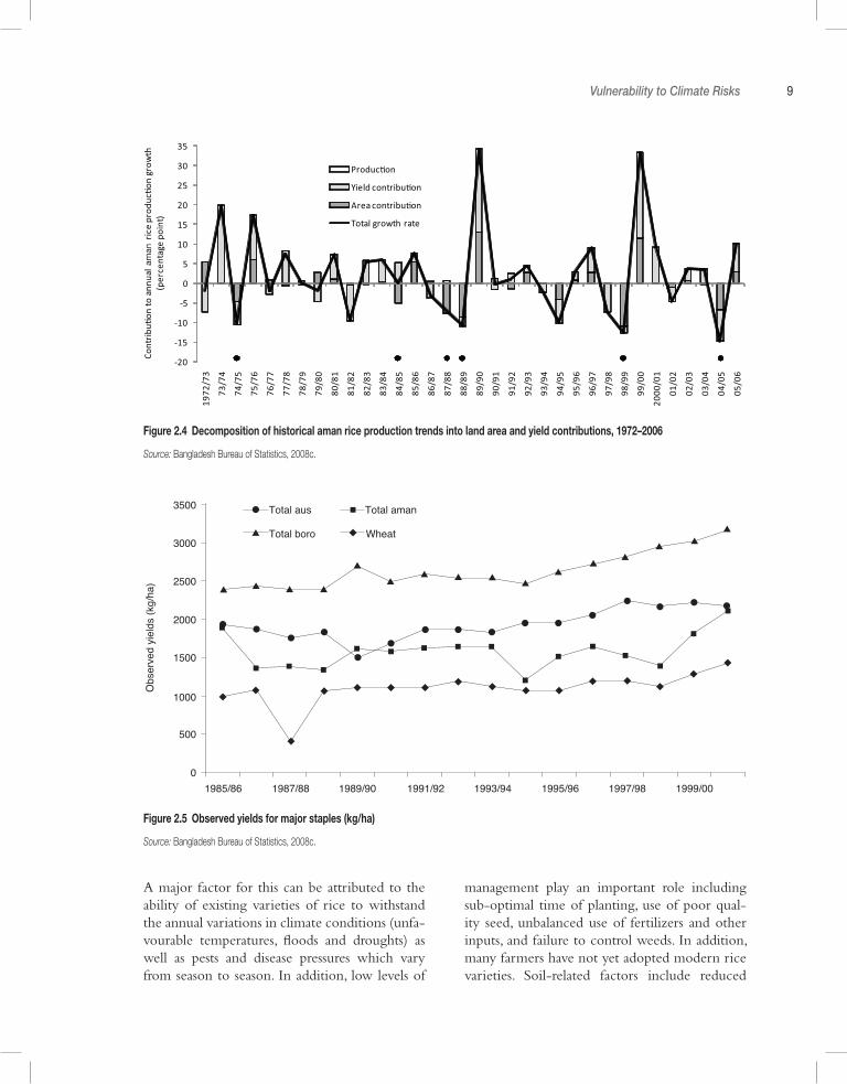
Figures1.1 Multi-stage integrated framework methodology 32.1 Agricultural and total GDP growth trends, 1975–2008 72.2 Historical trends in rice production quantities in Bangladesh, 1972–2006 82.3 Historical trends in land area under rice cultivation in Bangladesh, 1972–2006 82.4 Decomposition of historical Aman rice
production trends into land area and yield contributions, 1972–2006 92.5 Observed yields for major staples (kg/ha) 92.6 Time-series of flood-affected areas (km2) in Bangladesh (1954–2004) 112.7 Annual and seasonal precipitation time-series (mm) averaged across Bangladesh Meteorological Department stations 122.8 Average discharges in 1998 and 2002 for (a) Brahmaputra, (b) Ganges and (c) Meghna rivers 132.9 Cropping calendar corresponding to flood land type 142.10 Aman crop production loss curve as a function of combined discharge 162.11 Locations of coastal water level stations 172.12 Ganges-Brahmaputra-Meghna river basin 203.1 Monthly, annual and seasonal temperature changes 243.2 Monthly, annual and seasonal precipitation changes 254.1 Validated discharges from 1998–2007 at (a) Bahadurabad (b) Hardinge Bridge 294.2 Temperature changes for A2 scenario over GBM basin (the 2050s) 32
4.3 Percentage change in discharges in (a) the 2030s and (b) the 2050s for A2 scenario in August 334.4 Percentage change in discharges in (a) the 2030s and (b) the 2050s for A2 scenario in May 344.5 Total change in national flooded area for (a) 2030s A2, (b) 2030s B1, (c) 2050s A2, (d) 2050s B1 364.6 Yearly peak levels at Jamuna station for the baseline and model experiments (2030s) 374.7 Average hydrographs (baseline, 2030s,
2050s) for MIROC GCM and A2 scenario on Teesta River 384.8 Average hydrographs (baseline, 2030s,
2050s) for GFDL GCM and A2 scenario on Meghna River 384.9 Average hydrographs on the Gorai River (baseline, 2030s, and 2050s – for CCSM A2 scenario) and plus/ minus one standard deviation bounds 395.1 Baseline sub-regional yields with flood damages applied (as a percentage of undamaged yields) 485.2 Percentage change (versus the baseline undamaged simulation) in national potential production of a) aus, b) aman, c) boro and d) wheat 505.3 Percentage change (versus the baseline flood-only simulation) in national potential production affected by basin floods of a) aus and b) aman
(boro and wheat are assumed to be flood-free) 535.4 Percentage of production lost to coastal inundation associated with sea level rise in each coastal region sub-region (9–16) for three future
scenarios, as compared to the baseline period (for A2 SRES) 54

viii Climate Change Risks and Food Security in Bangladesh
5.5 Percentage change (versus the baseline flood-affected simulation) in
national potential production with the combined effects of CO2, temperature
and precipitation, and basin flooding of a) aus, b) aman, c) boro and d) wheat 555.6 Regional production changes from
baseline (per cent) for 2050s (a) aman, (b) aus, (c) boro and (d) wheat 576.1 Losses in total national rice production due to existing climate variability, 2005–50 666.2 Losses in national rice production by crop due to existing climate variability, 2005–50, (a) aus, (b) aman, (c) boro 676.3 Decomposing regional rice production losses due to existing climate variability, 2005–50 696.4 Losses in national agricultural GDP due to existing climate variability, 2005–50 696.5 Losses in national total GDP due to existing climate variability, 2005–50 716.6 Losses in total national rice production due to climate change, 2005–50 736.7 Losses in national rice production by crop due to climate change, 2005–50 756.8 Deviation in average final year rice
production from the Existing Variability Scenario under the Average Climate
Change Scenario, 2050 766.9 Deviation in average final year rice
production from the Existing Variability Scenario under different emissions
scenarios, 2050 766.10 Losses in national agricultural GDP due to climate change, 2005–50 776.11 Losses in national total GDP due to climate change, 2005–50 796.12 Cumulative discounted losses due to
climate change as a share of total GDP, 2005–50 807.1 Layout of modified sorjan system 88
Tables2.1 Production of different crop varieties (metric tons) 62.2 Flood classifications 102.3 Comparison of losses resulting from recent large floods 11
2.4 Peak discharge and timing during extreme flood years 122.5 Typical crop calendar for four different rice varieties 142.6 Hydrological regions and flood land types 152.7 Summary of drought severity areas in Bangladesh by crop season (in Mha) 162.8 Estimated trends in water level of different stations along the coastline 182.9 Area affected by low, moderate and high salinity level (in 2005) 193.1 IPCC AR4 global circulation models 223.2 Summary precipitation statistics averaged across Bangladesh (1960–2001) 263.3 Sea level rise impacts on flood land types 264.1 The sub-regions with hydrological region, agro-ecological zone and districts 324.2 Estimated average change (per cent) in discharge across all model experiments 334.3 Modelled baseline season flood land type distribution for each month (ha) 354.4 Protected areas flood control and drainage infrastructure (FCDI) 354.5 Number of model experiments exceeding one standard deviation bounds on baseline (2030s/2050s) and 2050s average estimated change in area flooded 364.6 Peak water level summary for the 2050s 375.1 Sub-regional agricultural information 435.2 Climate information for each sub- region: the representative BMD station, its code and annual mean climate statistics during the 1970–99 baseline period 445.3 Soil profile information for each sub-region 445.4 Agriculture management options for
simulations of the three main rice varieties 455.5 Agriculture management options for wheat simulations 465.6 Flood damages (percentage yield)
according to submergence depth, duration and phenological stage 475.7 Representative hydrographs 48
5.8 Carbon dioxide concentrations (ppm) for baseline period and future climate
scenarios 515.9 Median integrated production change (per cent) for the 2030s and 2050s 545.10 Sub-regional average production changes (per cent) disaggregated by crop (aman, aus, boro, wheat) and climate risk for 2050s – all scenarios 586.1 Summary of the Optimal Climate Scenario 656.2 National rice production losses due to existing climate variability, 2005–50 666.3 Regional rice production losses due
to existing climate variability, 2005–50 686.4 Losses in GDP due to existing climate variability, 2005–50 706.5 Losses in national households’
consumption spending due to existing climate variability, 2005–50 726.6 National rice production losses due to climate change, 2005–50 746.7 Average GDP losses due to climate change, 2005–50 786.8 GDP losses under different climate change scenarios, 2005–50 786.9 Losses in national households’
consumption spending due to climate change, 2005–50 806.10 Losses in regional farm households’
consumption spending due to climate change, 2005–50 817.1 Sample of past and present programmes on adaptation in the agriculture sector 847.2 Sample adaptation options in the agriculture sector 847.3 Estimated costs and benefits of selected adaptation options 857.4 Common vegetable cultivation patterns 1017.5 Common vegetable cropping patterns for sorjan system 104
A1.1 Cultivars available in the DSSAT v4.5 CERES-Rice model 108A1.2 Genetic coefficients in the DSSAT v4.5 CERES-Rice model 109A1.3 Cultivars available in the DSSAT v4.5 CERES-Wheat model 109A1.4 Genetic coefficients in the DSSAT v4.5 CERES-Wheat model 109A1.5 Planting method options in the DSSAT v4.5 models 110A1.6 Tillage implements available in the DSSAT v4.5 models 110A1.7 Irrigation options in the DSSAT v4.5 models 111A1.8 Fertilizer types in the DSSAT v4.5 models 111A1.9 Fertilizer and organic amendment
application options in the DSSAT v4.5 models 111A1.10 Organic amendments available in the DSSAT v4.5 models 111A2.1 Simple CGE model equations 114A2.2 Simple CGE model variables and parameters 115A2.3 Summary of climate impact channels in economy-wide model simulations 116A3.1 Basic structure of a SAM 120A3.2 Sectors in the 2005 Bangladesh SAM 122A3.3 Average cultivated crop land allocation across divisions and scale of production 123A3.4 National and divisional per cent of gross domestic product (GDP) 124A3.5 Household factor income shares from the 2005 Bangladesh SAM 125A3.6 Household factor income shares from the 2005 Household Income and Expenditure Survey 125A3.7 Household consumption 126A3.8 2005 macro SAM for Bangladesh (millions of Taka) 127A3.9 Cross-entropy SAM estimation equations 131
List of Figures and Tables ix

Acknowledgements
This report was prepared by a team led by Winston H. Yu (Task Team Leader, World Bank). Specific team contributions included: Mozaharul Alam, Rabi Uzzaman, Aminur Rahman (Bangla-desh Center for Advanced Studies) and Sk. Ghulam Hussain (Bangladesh Agricultural Research Council), who identified and evaluated the adapta-tion options present in this study and pro-vided agricultural information for crop models; Ahmadul Hassan, Bhuiya Md. Tamim Al Hossain, Mohammad Ragib Ahsan, Ehsan Hafiz Chowd-hury and Giasuddin Ahmed Choudhury (Center for Environmental and Geographic Information Systems), who provided an analysis of the historical hydrology of the country; Abu Saleh Khan, Sardar M Shah-Newaz, Sohel Masud and Emaduddin Ahmad (Institute of Water Modelling), who devel-oped the models used to project changes in future flooding; Alex C. Ruane, Cynthia Rosenzweig, David C. Major, Radley Horton and Richard Goldberg (Columbia University), with the advice of Md Sohel Pervez, who provided the future cli-mate scenarios and developed the models used to project future crop production; and James Thurlow and Paul Dorosh (International Food Policy Research Institute), who developed the computable general equilibrium model.
The authors benefited enormously from the many technical discussions with colleagues and Government of Bangladesh officials. Spe-cific reviewers included: Richard Damania, Julia Bucknall, Abel Lufafa, Ian Noble, Nagaraja Harshadeep, and Anna Bucher (from the World Bank), Abu Wali Raghib Hassan, Md Mahsin, Sanjib Saha, Md Abul Hossain, Mazharul Aziz, Mohammad Ataur Rahman, and Bilkish Begum
(from the Department of Agriculture Exten-sion), M. Akkas Ali (from the Bangladesh Agri-cultural Research Institute), Jiban Krishna Biswas (from the Bangladesh Rice Research Institute), Mahmuder Anwar, Zahangir Alam, and Razaul Hoque (from the Agricultural Information Serv-ice), and Ad Spijkers, Dr C.S. Karim, Tommaso Alacevich, Ciro Fiorillo, and Z Karim (from the Food and Agriculture Organization). Brooke Yamakoshi, Michael Westphal, and Siobhan Murray (World Bank) also provided valuable technical assistance during this study.
Finally, the authors are grateful for the sup-port of the World Bank management team and several of the Bangladesh country office staff including: Zhu Xian (former Country Director), Robert Floyd, Adolfo Brizzi, Gajan Pathmanathan, John Henry Stein, Simeon Ehui, Karin Kemper, Masood Ahmad, Nihal Fernando, S.A.M. Rafiquz-zaman, Shakil Ferdausi and Khawaja Minnatul-lah. Ryma Aguw, Tarak Chandra Sarker, Venkat Ramachandran and Talat Fayziev helped in the administration of this study. The photographs of various adaptation options were provided by the Department of Agricultural Extension, Ministry of Agriculture, Bangladesh and the Livelihood Adap-tation to Climate Change (LACC-II) Project.
Generous support for this study was pro-vided by the World Bank, the Global Facility for Disaster Reduction and Recovery (GFDRR), the Trust Fund for Environmentally and Socially Sustainable Development (TFESSD), the Eco-nomics of Adaptation to Climate Change (EACC) study team, and the Bank-Netherlands Water Partnership Program (BNWPP). We also acknowledge the Program for Climate Model

xii Climate Change Risks and Food Security in Bangladesh
Diagnosis and Inter-comparison (PCMDI) and the WCRP Working Group on Coupled Model-ling (WGCM) for their roles in making available the WCRP CMIP3 multi-model dataset. Sup-port of this dataset is provided by the Office of Science, US Department of Energy.
This study is a product of the staff and con-sultants of the World Bank. The findings, interpre-tations, and conclusions expressed in this paper do not necessarily reflect the views of the Execu-tive Directors of The World Bank or the govern-ments they represent.
Foreword
This report is an important first step in better understanding how climate risks (both cur-rent and future) can undermine food security in Bangladesh. It identifies key areas that require concerted effort by the government and its many development partners.
The year 2007 was indicative of the develop-ment challenges that Bangladesh faces. Severe flooding from July to September 2007 along the Ganges and Brahmaputra rivers affected over 13 million people in 46 districts and caused extens-ive damage to agricultural production and physi-cal assets. With hardly any time to recover, on 15 November 2007 the deadly Cyclone Sidr, a cate-gory IV storm, made landfall across the southern coast of the country, causing over 3000 deaths. The economic damages amounted to over US$1 billion, with over a million tons of rice destroyed. Then, the increase in international prices of oil and food, which Bangladesh imports, put further strains on both government budgets and house-hold livelihoods.
The long-term economic consequences of these three simultaneous shocks remain to be seen, but they have shown the inherent vulnerability of Bangladesh to climate risks and the degree to which food security remains a major challenge for the country. With too much water during the heavy monsoon months and too little water during the spring and early summer months, communities have needed to adapt to changing conditions. They have done so by adopting new varieties of crops and new farming practices and by starting small businesses and trades to diver-sify incomes. Furthermore, over the last several decades the government has invested heavily and
wisely to protect its citizenry to ensure growth and a prosperous nation. This includes invest-ments in infrastructure, including embankments and cyclone shelters which have saved count-less numbers of lives, in early warning systems to help the country prepare for imminent disasters, and polders to protect vital agricultural areas to maintain production to feed its population. The gains from these investments continue to support a growing nation.
Climate change, however, threatens to offset to some degree these important advances. The prospect of changing temperatures and precipita-tion patterns, the uncertainty of the timing and magnitude of extreme events, and rising sea levels will have important impacts on the agriculture sector. Action is needed today because Bangla-desh will continue to depend on the agriculture sector for growth and poverty reduction. Invest-ments from the public and private sectors will have to increase if Bangladesh is to ensure food security for its current and future populations.
The challenges that the agriculture sector will face as it adapts to climate change coincide well with the needs required to address the climate variability risks of today. Thus, the adaptation options identified are no-regret approaches and only a small example of what is possible. I hope that this report can serve as a useful and mean-ingful guide for Bangladesh (and other countries) in addressing a future uncertain world.

Executive Summary
Background
Bangladesh is one of the countries most vulnerable to climate risks
From annual flooding to a lack of water during the dry season, from frequent coastal cyclones and storm surges to changing groundwater aquifer conditions, the importance of adapting to climate risks to maintain economic growth and reduce poverty is clear. Households have for a long time needed to adapt to these dynamic conditions to maintain their livelihoods. Moreover, substantial public investment in protective infrastructure (e.g. cyclone shelters, embankments) and early warning and preparedness systems has played and will continue to play a critical role in minimizing these impacts. In the long list of potential impacts from climate change, the risks to the agriculture sector stand out as among the most important.
Agriculture is a key economic sector in Bangladesh, accounting for nearly 20 per cent of the GDP (gross domestic product) and 65 per cent of the labour force
The performance of the sector has considerable influence on overall growth, the trade balance, the budgetary position of the government, and the level and structure of poverty and malnutri-tion in the country. Moreover, much of the rural population, especially the poor, is reliant on the agriculture sector as a critical source of livelihood and employment. Many also depend on the agri-culture sector indirectly through employment in small-scale rural enterprises that provide goods and services to farms and agro-based industries and trades.
Climate is only one input factor in a sector that is already under pressure
The achievement of food self-sufficiency remains a key development agenda for the country. Sig-nificant progress has been made in the sector since the 1970s, in large part due to the rapid expansion of surface and groundwater irriga-tion and the introduction of new high-yielding crop varieties. The production of rice and wheat increased from about 10 million tonnes/metric tons (10Mt) in the early 1970s to almost 30Mt by 2001. The challenge now for Bangladesh is to enhance productivity, especially as demands for food increase with the growing population (1.3 per cent growth rate) and improved incomes. Moreover, overuse, degradation and changes in resource quality (e.g. salinity) will place addi-tional pressures on already constrained available land and water resources.
Climate change is recognized as a key sustainable development issue for Bangladesh
Future climate change risks will be additional to the challenges the country and sector already face. Long-term changes in temperatures and precipitation have direct implications on evapora-tive demands and consequently on agriculture yields. Moreover, water-related disasters may increase in magnitude and frequency. Finally, sea level rise may have important implications for the sediment balance and may alter the profile of the area inundated and salinity in the coastal areas.
xvi Climate Change Risks and Food Security in Bangladesh
The objective of this study is to examine the implications of climate change on food security in Bangladesh and to identify adaptation measures in the agriculture sector
This objective is achieved in the following ways. First, the most recent science available is used to characterize current climate and hydrology and its potential changes. Second, country-specific survey and biophysical data is used to derive more realistic and accurate agricultural impact functions and simulations. A range of climate risks (i.e. warmer temperatures, higher carbon dioxide concentrations, changing characteristics of floods, droughts and potential sea level rise) is considered to gain a more complete picture of potential agriculture impacts. Third, while estimating changes in production is impor-tant, economic responses may to some degree buffer against the physical losses predicted, and an assessment is made of these. Food security is dependent not only on production stocks, but also future food requirements, income levels and commodity prices. Fourth, adaptation possibili-ties are identified for the sector. The framework established here can be used effectively to test such adaptation strategies. Multiple models are used in this integrated study, and as with all mod-els, parameters may not be known with precision and functional forms may not be fully accurate; thus, careful sensitivity analysis and a full under-standing of limitations (identified throughout the study) are required.
Vulnerability to Climate Risks (Chapter 2)
The performance of the agriculture sector is heavily dependent on the characteristics of the annual flood
Regular flooding of various types (e.g. flash, river-ine) has traditionally been beneficial. However, low frequency but high magnitude floods can have adverse impacts on rural livelihoods and production (e.g. the 1998 flood resulted in a loss of over 2Mt of production). The timing of the peaks of the three major river systems (Ganges, Brahmaputra and Meghna) is an important deter-minant of the overall magnitude of flooding. The economy-wide impact of these extreme events can be substantial. Impacts on the ‘aman’ (mon-soon season rice) and ‘aus’ (inter-season rice) are
the primary drivers of declining overall produc-tion during major flood events (driven mainly by area changes); these losses, however, are increas-ingly being compensated for by ‘boro’ (dry sea-son rice). As a result, compared to the pre-1990s, agricultural GDP is becoming less sensitive to this climate variability. Finally, droughts and coastal inundation from sea level rise can have consequences for agriculture production as large as those from floods.
Future Climate (Chapter 3)
Using global climate models (GCMs), a trend toward a warmer and wetter future climate is projected to impact the agriculture sector, particularly if the climate state goes beyond the variations found in the historical record
Median warming of 1.1°C, 1.6°C and 2.6°C by the 2030s, 2050s and 2080s respectively is pro-jected from a range of plausible scenarios. Median annual precipitation increases of 1 per cent, 4 per cent and 7.4 per cent by the 2030s, 2050s and 2080s respectively is projected with greater con-trasts between the wet and dry seasons. Greater model uncertainty (in terms of magnitude and direction) exists with future precipitation than future temperature. Simulated future tempera-ture changes significantly separate from the background temperature variations. Precipitation is subject to large existing inter-annual and intra-annual variations. Projections of precipitation changes vary widely amongst models, with small median changes compared to historic variability. Using three scenarios of future sea level rise (15 cm, 27 cm, and 62 cm) the total area that peren-nially floods is projected to increase by 6%, 10%, and 20% respectively.
Future Floods (Chapter 4)
Primarily driven by increased monsoon precipitation in the Ganges-Brahmaputra-Meghna (GBM) basin, models on average demonstrate increased future flows in the three major rivers into Bangladesh (as much as 20 per cent)
Larger changes are anticipated by the 2050s com-pared to the 2030s. Larger changes are observed on average for the Ganges. The exact magnitude is dependent on the month. Given that most
GCMs project both an increasing trend of mon-soon rainfall and greater inflows into Bangla-desh, it follows that the flooding intensity would worsen. On average, models simulate increases in flooded area in the future (over 10 per cent by 2050). This is primarily located in the central part of the country at the confluence of the Ganges and Brahmaputra rivers and in the south.
Moreover, increases in yearly peak water lev-els are projected for the northern sub-regions and decreases are projected for the southern sub-regions. Not all estimated changes are statisti-cally significant. Model experiments demonstrate more changes that are significant by the 2050s. Changes are in general less than 0.5m from the baseline. Furthermore, across the sub-regions, most GCMs show earlier onset of the monsoon and a delay in the recession of flood waters.
Future Crop Performance (Chapter 5)
The median of all rice crop projections shows declining national production, with boro showing the largest median losses
Potential future crop production is projected using well-developed crop models considering multiple climate impacts (temperature and pre-cipitation changes, CO
2 fertilization, flood
changes, sea level rise). For aus (-1.5 per cent) and aman (-0.6 per cent) the range of model experiments for the 2050s covers both potential gains and losses and does not statistically sepa-rate from zero. However, most GCM projections estimate a potential decline in boro production with a median loss of 3 per cent by the 2030s and 5 per cent by the 2050s. Wheat production is projected to increase out to the 2050s (+3 per cent). Boro and wheat changes are conservative as it is assumed that farmers have unconstrained access to irrigation. In each sub-region, produc-tion losses are estimated for at least one crop. The production in the southern sub-regions is most vulnerable to climate change. For instance, average losses in the Khulna region are -10 per cent for aus, aman and wheat, and -18 per cent for boro by the 2050s due in large part to ris-ing sea levels. These production impacts ignore economic responses to these shocks (e.g. land
and labour reallocation, price effects). These eco-nomic effects will to some degree buffer against the physical losses predicted.
Economy-wide Impacts of Climate Risks (Chapter 6)
Existing climate variability can have a pronounced detrimental economy-wide impact
This is explored using a dynamic computable general equilibrium (CGE) model. Compared to an ‘optimal’ climate simulation in which highest simulated yields are used and sector productiv-ity and factor supplies increase smoothly at aver-age long-term growth rates with no inter-annual variations, climate variability is estimated to reduce long-term rice production by an average 7.4 per cent each year over the 2005–50 simu-lation period. This primarily lowers the produc-tion of the aman and aus crop. Average annual rice production growth is lowered in all sub-regions. This simulated variability is projected to cost the agriculture sector (in discounted terms) US$26 billion in lost agricultural GDP during the 2005–50 period. This climate variability has economy-wide implications beyond simply the size-effect of the lost agricultural GDP. Existing climate variability is estimated to cost Bangladesh US$121 billion in lost national GDP during this period (US$3 billion per year). This is 5 per cent below what could be achieved if the climate were ‘optimal’.
Climate change exacerbates the negative impacts of existing climate variability by further reducing rice production by a projected cumulative total of 80Mt over 2005–50 (about 3.9 per cent each year), driven primarily by reduced boro crop production
This is equivalent to almost 2 years worth of rice production lost over the next 45 years as a result of climate change. Uncertainty about future cli-mate change means that annual rice production losses range between 3.6 per cent and 4.3 per cent. Climate change has particularly adverse implications for boro rice production and will limit its ability to compensate for lost aus and aman rice production during extreme climate events. This will further jeopardize food security
Executive Summary xvii
xviii Climate Change Risks and Food Security in Bangladesh
in Bangladesh, necessitating greater reliance on other crops and imported food grains. Rice pro-duction in the southern regions of Patuakhali and Khulna is particularly vulnerable.
Overall, agricultural GDP is projected to be 3.1 per cent lower each year as a result of climate change (US$7.7 billion in lost value-added)
Climate change also has broader economy-wide implications. This is estimated to cost Bangladesh US$26 billion in total GDP over the 45-year period 2005–50, equivalent to US$570 million overall lost each year due to climate change, or alternatively an average annual 1.15 per cent reduction in total GDP. Average loss in agri-cultural GDP due to climate change is projected to be a third of the agricultural GDP losses asso-ciated with existing climate variability. Uncer-tainty surrounding GCMs and emission scenarios means that costs may be as high as US$1 billion per year in 2005–50 under less optimistic sce-narios. Moreover, these economic losses are pro-jected to rise in later years, thus underlining the need to address climate change related losses in the near-term.
These climate risks will also have severe implications for household welfare
For both the climate variability and climate change simulations, around 80 per cent of total losses fall directly on household consumption (cumulative total consumption losses of US$441.7 billion and US$104.7 billion for climate variability and cli-mate change simulations respectively). Also, about 80 per cent of the economic losses occur outside of agriculture, particularly in the upstream and downstream agriculture value-added processing sectors. This means that both rural and urban households are adversely affected. Per capita con-sumption is projected to fall for both farm and non-farm households.
The southern and northwest regions are the most vulnerable
The south sits at the confluence of multiple cli-mate risks, as shown throughout this study. These areas are expected to experience the largest decline
in rice production due to climate change. This is for three reasons. First, these regions already experience significant declines in aus and aman rice production due to climate variability, which is expected to worsen under climate change. Sec-ond, boro yields are severely affected by changes in mean rainfall, temperature and mean shifts in the flood hydrographs. Thus, reductions in boro production limit the ability for these regions to compensate for lost aus and aman rice production during extreme events. The south is also affected the most by rising sea levels, which permanently reduce cultivable land. The largest percentage declines in per capita consumption are projected in these regions. Finally, the northwest is also vul-nerable as the lost consumption is a large fraction of the existing household consumption. Adapta-tion measures should focus on these areas.
Adaptation Options in the Agriculture Sector (Chapter 7)
Adaptation options can address several different climate risks
Bangladesh will continue to depend on the agri-culture sector for economic growth. Rural house-holds will continue to depend on the agriculture sector for income and livelihoods. Though the government has made substantial investments to increase the resilience of the poor (e.g. new high-yielding crop varieties, protective infrastructure, disaster management), existing constraints in the sector may be exacerbated by long-term effects of climate change. The scale of current efforts remains limited and is not commensurate with the probable impacts. A no-regrets strategy is to promote activities and policies that help house-holds build resilience to existing climate risks today.
Both processes of adapting to climate change and stimulating the agriculture sector to achieve rural growth and support livelihoods align well.
This requires, among other things, efforts to: diversify household income sources; improve crop productivity; support greater agricultural research and development; promote education and skills development; increase access to finan-
cial services; enhance irrigation efficiency and overall water and land productivity; strengthen climate risk management; and develop protec-tive infrastructure. Moreover, the current large gap between actual and potential yields suggests substantial on-farm opportunities for growth and poverty reduction. Expanded availability of mod-ern rice varieties, irrigation facilities, fertilizer use and labour could increase average yields at rates that could more than offset the climate change impacts. Significant additional planning and investments in promoting these types of adapta-tions are still needed.
The Way Forward (Chapter 8)
The precise impact of climate change on coun-tries in the developing world remains to be seen. This much is known, however: climate change poses additional risks to many developing coun-tries in their efforts to reduce poverty, promote
Executive Summary xix
livelihoods and develop sustainably. As popula-tions grow, the ability for many countries to meet basic food requirements and effectively manage future disasters will be critical for sus-taining long-term economic growth. These are challenges above and beyond those that many countries are already currently facing.
The integrated framework used in this analy-sis provides a broad and unique approach to esti-mating the hydrologic and biophysical impacts of climate change, the macro-economic and house-hold-level impacts and an effective method for assessing a variety of adaptation practices and policies. The framework presented here can serve as a useful guide to other countries and regions faced with similar development challenges and objectives of achieving food security. Continued refinements to the assessment approach devel-oped in this volume will further help to sharpen critical policies and interventions by the Bangla-desh government.

Glossary of Terms
B. aman: broadcast aman; a rice crop usually planted in March/April under dry land condi-tions, but in areas liable to deep flooding. Also known as deep water rice. This crop is harvested from October to December. All varieties are highly sensitive to day length.
T. aman: transplanted aman; a rice crop usually planted in July/August, during the monsoon, in areas liable to a maximum flood depth of about 0.5m. This crop is harvested from November/December. Local varieties are sensitive to day length whereas modern varieties are insensitive or only slightly sensitive.
B. aus: broadcast aus; a rice crop planted in March/April under dry land conditions. Matures on pre-monsoon showers, harvested in June/July, and is insensitive to day length.
T. aus: transplanted aus; a rice crop, transplanted in March/April, usually under irrigated condi-tions, and harvested June/July. The distinction between late planted boro and early transplanted aus is academic since the same varieties may be used. Varieties are insensitive to day length.
Boro: a rice crop planted under irrigation dur-ing the dry season from December to March and harvested in April to June. Local boro varieties are more tolerant of cool temperatures and are usually planted early in areas which are subject to early flooding due to rise in river levels. Improved varieties, less tolerant of cool conditions, are usu-ally transplanted from February onwards. All varieties are insensitive to day length.
Kharif: the wet season (typically March to Octo-ber) characterized by monsoon rain and high temperatures.
Kharif 1: the first part of the kharif season (March to June). Rainfall is variable and temper-atures are high. The main crops grown are Aus, summer vegetables and pulses. Broadcast aman and jute are planted.
Kharif 2: the second part of the kharif season (July to October) characterized by heavy rain and floods. T. aman is the major crop grown during the season. Harvesting of jute takes place. Fruits and summer vegetables may be grown on high land.
Rabi: The dry season (typically November to February) with low or minimal rainfall, high evapo-transpiration rates, low temperatures and clear skies with bright sunshine. Crops grown are boro, wheat, potato, pulses and oilseeds.
High yielding variety: introduced varieties developed through formal breeding programmes, they have a higher yield potential than local varie-ties but require correspondingly high inputs of fertilizer and irrigation water to reach full yield potential.
Local varieties developed and used by farm-ers: Sometimes referred to as inbred varieties or local improved varieties (LIVs).
Net cultivable area: total area which is under-taken for cultivation.

Acronyms
AIS Agricultural Information Service
AR4 Fourth Assessment Report
BARC Bangladesh Agricultural Research Council
BARI Bangladesh Agricultural Research Institute
BBS Bangladesh Bureau of Statistics
BCAS Bangladesh Centre for Advanced Studies
BINA Bangladesh Institute of Nuclear Agriculture
BMD Bangladesh Meteorological Department
BRRI Bangladesh Rice Research Institute
BWDB Bangladesh Water Development Board
CEGIS Center for Environmental and Geographic Information Services
CERES Crop Environment Resource Synthesis
CGE computable general equilibrium
CO2 carbon dioxide
DAE Department of Agriculture Extension
DEM digital elevation model
DSSAT Decision Support System for Agrotechnology Transfer
ENSO El Niño-Southern Oscillation
FAO Food and Agriculture Organization
FCDI Flood control and drainage infrastructure
FFWC Flood Forecast and Warning Center
GBM Ganges-Brahmaputra-Meghna
GCM global climate model
GDP gross domestic product
GOB Government of Bangladesh
GTOPO Global Topography
HIES Household Income and Expenditure Survey
HYV high yielding variety
IFPRI International Food Policy Research Institute
IMF International Monetary Fund
IPCC Intergovernmental Panel on Climate Change
IWM Institute of Water Modelling
LACC Livelihood Adaptation to Climate Change
MJO Madden-Julian Oscillation
Mt million tonnes (million metric tons)
MPO Master Plan Organization
MSL mean sea level
NASA National Aeronautics and Space Agency
NCA net cultivable area
NGO non-governmental organization
PCMDI Program for Climate Model Diagnosis and Inter-comparison
RCM regional climate model

xxiv Climate Change Risks and Food Security in Bangladesh
SAM social accounting matrix
SRES Special Report on Emissions Scenario
SRTM Shuttle Radar Topography Mission
TAR Third Assessment Report
TRMM Tropical Rainfall Measuring Mission
USGS United States Geologic Survey
1
Introduction
Bangladesh is one of the most vulnerable countries to climate risks, both from existing variability and future climate change. From annual flooding of all types to a lack of water resources during the dry season, from frequent coastal cyclones and storm surges to changing groundwater aquifer condi-tions, the importance of adapting to these risks to maintain economic growth and reduce poverty is clear. Households have for a long time needed to adapt to these dynamic conditions to maintain their livelihoods. The nature of these adaptations and the determinants of success depend on the availability of assets, labour, skills, education, and social capital. The relative severity of disasters has decreased substantially since the 1970s, however, as a result of improved macro-economic manage-ment, increased resilience of the poor and signifi-cant progress in disaster management. Substantial public investment in protective infrastructure (e.g. cyclone shelters, embankments) and early warning and preparedness systems have played a critical role in minimizing these impacts. More investments are still required. In the long list of potential impacts from climate change, the risks to the agriculture sector stand out as among the most important.
Agriculture is a key economic sector in Bang-ladesh, accounting for nearly 20 per cent of the GDP and 65 per cent of the labour force. The performance of the sector, here to include crops (70 per cent of agricultural GDP), livestock (10 per cent) and fisheries (10 per cent), has con-siderable influence on overall growth, the trade balance, the budgetary position of the govern-ment, and the level and structure of poverty and malnutrition in the country. Moreover, much of
the rural population, especially the poor, is reliant on the agriculture sector as a critical source of livelihoods and employment. Many may also do so indirectly through employment in small-scale rural enterprises that provide goods and services to farms and agro-based industries and trades.
Climate is only one input factor in an agri-culture sector that is already under pressure. The achievement of food self-sufficiency remains a key development goal for the country. Significant progress has been made in the sector since the 1970s, in large part due to the rapid expansion of surface and groundwater irrigation and the introduction of new high-yielding crop varieties. The production of rice and wheat increased from about 10 million tonnes/metric tons (10Mt) in the early 1970s to almost 30Mt by 2001. The challenge now for Bangladesh is to enhance pro-ductivity, especially as demands for food increase with the growing population (1.3 per cent growth rate) and improved incomes. Moreover, overuse, degradation and changes in resource quality (e.g. salinity) will place additional pressures on already constrained available land and water resources.
Future climate change risks will be additional to the challenges the country and sector already face. Long-term changes in temperatures and pre-cipitation have direct implications on evaporative demands and consequently on agriculture yields. Increased carbon dioxide concentrations may also impact the rates of photosynthesis and respiration. Moreover, water-related disasters may increase in magnitude and frequency. In fact, between 1991 and 2000, 93 major disasters were recorded, result-ing in billions of US$ in losses, most of which were in the agriculture sector. Sea level rise may
2 Climate Change Risks and Food Security in Bangladesh
have important implications on the sediment bal-ance and may alter the profile of available land for production in the coastal areas. It is clear that climate change is a key sustainable development issue for Bangladesh (World Bank, 2000).
1.1 Objective of StudyThe objective of this study is to examine the implications of climate change on food secu-rity in Bangladesh and to identify adaptation measures in the agriculture sector. This objec-tive is achieved in the following ways. First, the most recent science available is used to charac-terize current climate and its potential changes. Second, country-specific survey and biophysical data is used to derive more realistic and accu-rate agricultural impact functions and simula-tions. A range of climate risks (i.e. warmer tem-peratures, higher carbon dioxide concentrations, changing characteristics of floods, droughts and potential sea level rise) is considered, to gain a more complete picture of potential agriculture impacts. Third, while estimating changes in pro-duction is important, this is only one dimension of food security considered here. Food security is dependent on several socio-economic variables including estimated future food requirements, income levels and commodity prices. Fourth, adaptation possibilities are identified for the sec-tor. The framework established here can be used effectively to test such adaptation strategies.
1.2 Literature ReviewGlobal changes in climate will have important implications for the economic productivity of the agriculture sector. The sector will be impacted by three primary water-related climate drivers. First, gradual changes in the distribution of precipi-tation and temperature will impact agriculture yield through possible changes in water availabil-ity and evaporative demands, tolerance of crops and incidence of pest attacks. Second, changes in the frequency and magnitude of extreme events (i.e. above-average floods, prolonged droughts) may result in additional shocks to the agriculture sector. The ability to recover from these short-
term production losses and the impacts on long-term prospects is dependent on many macro and micro factors. Third, the prospects of sea level rise in the coastal areas will change the profile of available land for agriculture production and potentially the quality of groundwater used for irrigation. This is especially critical in land-con-strained countries such as Bangladesh. Increases in carbon dioxide concentrations will also impact the rates of photosynthesis and respiration.
Much of the existing analysis on climate change impacts on the agriculture sector has pri-marily been focused on the first driver: changes in temperature and precipitation. Several global studies look at these impacts. For instance, Cline (2007) demonstrates using a range of method-ologies and several global circulation models (GCMs) that agriculture production may decline in Bangladesh by as much as between 15 and 25 per cent. This study is dependent on global sta-tistical production functions. Fischer et al (2002) derive similar estimates using an agro-ecological approach and the results from four global circula-tion models.
Several regional level studies also exist which show mixed responses to climate change. Lal et al (1998a,b,c) demonstrate that rice yields in neigh-boring India could decline by 5 per cent under a 2°C warming and CO
2 doubling. Karim et al
(1994) indicated a decrease in potential yields for aman and boro rice in Bangladesh when only a 2°C or 4°C temperature change is considered, but this decrease was nearly offset when the physio-logical effect of 555 parts per million (ppm) CO
2
fertilization was taken into account. More recent results (Karim et al, 1998; Faisal and Parveen, 2003) show overall enhancement of potential rice yields but declines in potential wheat yields when 4°C temperature changes and 660ppm CO
2 fertilization are simulated. The offset poten-
tial by carbon fertilization effects remains an area of active research (Long et al, 2005;IPCC, 2007b; Tubiello et al, 2007a,b; Hatfield et al, 2008; Ains-worth et al, 2008).
Although it is clear that floods can affect agriculture production significantly, little is known about the incremental future damages from more frequent extreme events or increased
Introduction 3
discharges. Economic damages have been cal-culated after several recent extraordinary flood events (e.g. almost US$700 million in agriculture losses were reported after floods in 2004). Hus-sain (1995) developed a methodology to incor-porate yield losses from annual flooding into a crop simulation model. Sea level rise and salinity intrusion implications on the agriculture sector are even less understood. Habibullah et al (1998) calculated that the loss of food-grain due to soil salinity intrusion in the coastal districts is about 200,000 to 650,000 tons.
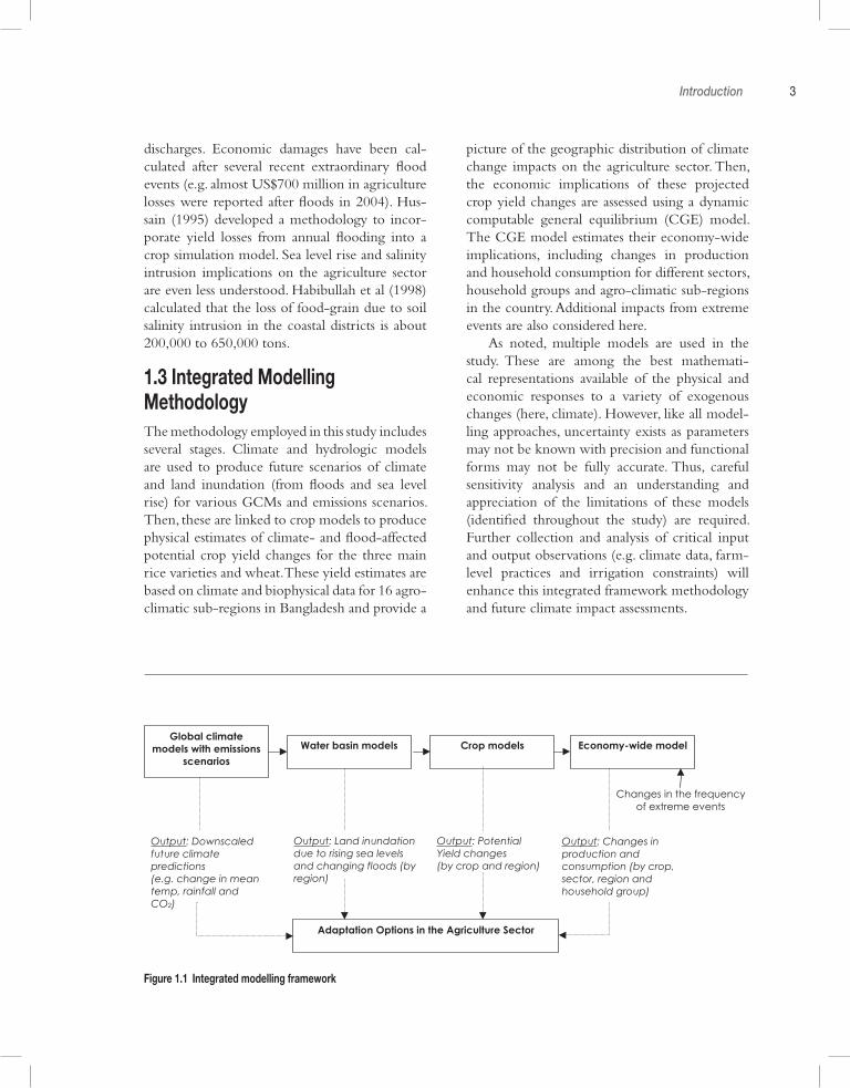
1.3 Integrated Modelling MethodologyThe methodology employed in this study includes several stages. Climate and hydrologic models are used to produce future scenarios of climate and land inundation (from floods and sea level rise) for various GCMs and emissions scenarios. Then, these are linked to crop models to produce physical estimates of climate- and flood-affected potential crop yield changes for the three main rice varieties and wheat. These yield estimates are based on climate and biophysical data for 16 agro- climatic sub-regions in Bangladesh and provide a
picture of the geographic distribution of climate change impacts on the agriculture sector. Then, the economic implications of these projected crop yield changes are assessed using a dynamic computable general equilibrium (CGE) model. The CGE model estimates their economy-wide implications, including changes in production and household consumption for different sectors, household groups and agro-climatic sub-regions in the country. Additional impacts from extreme events are also considered here.
As noted, multiple models are used in the study. These are among the best mathemati-cal representations available of the physical and economic responses to a variety of exogenous changes (here, climate). However, like all model-ling approaches, uncertainty exists as parameters may not be known with precision and functional forms may not be fully accurate. Thus, careful sensitivity analysis and an understanding and appreciation of the limitations of these models (identified throughout the study) are required. Further collection and analysis of critical input and output observations (e.g. climate data, farm-level practices and irrigation constraints) will enhance this integrated framework methodology and future climate impact assessments.
Figure 1.1 Integrated modelling framework
Output: Downscaled future climatepredictions(e.g. change in mean temp, rainfall and CO2)
Output: PotentialYield changes(by crop and region)
Output: Land inundationdue to rising sea levels and changing floods (byregion)
Output: Changes in production and consumption (by crop, sector, region and household group)
Global climate models with emissions
scenariosCrop models Water basin models
Adaptation Options in the Agriculture Sector
Economy-wide model
Changes in the frequencyof extreme events
4 Climate Change Risks and Food Security in Bangladesh
1.4 Organization of StudyThis study is organized into seven further chap-ters. Chapter 2 sets the historical context of cli-mate risks in Bangladesh. Past experience with floods, droughts, sea level rise and observed trends is reviewed. Broader regional issues are also briefly discussed. Chapter 3 reviews the predicted future changes in precipitation and temperature (both at the country level and at the Ganges-Brahmaputra-Meghna [GBM] river basin level). Chapter 4 presents an analysis on modelling the hydrology of future floods. This consists of both descriptions of a regional and national hydrologic models used and an analysis of the characteristics of the future floods both temporally and spatially. Among other aspects, the extent of the flood and the changes in the peak floods are analysed. A procedure for selecting a sub-set of global climate
models is also presented as all available climate models could not be used. Chapter 5 describes the dynamic biophysical crop production models used. Here, various impacts of different climate risks (floods, droughts and sea level rise) on agri-culture yields, focusing on rice and wheat, are incorporated. Chapter 6 describes a dynamic computable general equilibrium model used to evaluate the macro-economic and household welfare impacts of both climate variability and change-induced yield losses and gains. Chap-ter 7 presents potential adaptation options for the agricultural sector including unit costs that are currently being piloted in the field. Finally, in Chapter 8, the study concludes with general recommendations. Annexes provide additional information about using the crop models to test adaptation options and technical details of the CGE.
2
Vulnerability to Climate Risks
Box 2.1 Key messages
• Despite the challenging physiography and extreme climate variability, Bangladesh has made signifi-cant progress towards achieving food security. Investments in surface and groundwater irrigation and the introduction of high yielding crop varieties have played and will continue to play a key role in this.
• The performance of the agriculture sector is heavily dependent on the characteristics of the annual flood. Regular flooding of various types has traditionally been beneficial. However, low frequency but high magnitude floods can have adverse impacts on rural livelihoods and production.
• The timing of the peaks on the three major river systems (Ganges, Brahmaputra and Meghna) is an important determinant of the overall magnitude of flooding.
• The economic toll of these extreme events can be significant, the order of billions of US dollars.• Aman and aus rice are the primary drivers of declining overall production during major flood events,
which is increasingly being compensated for by boro rice. Agriculture share of total GDP is declining and is likely to continue to do so, thus increasingly insulating the country from these shocks.
• Lean-season water availability, particularly in the northwest, can have consequences on agriculture production comparable to floods.
• In coastal areas, agriculture productivity is affected by the surface and groundwater salinity distribution.• Future regional changes in the Ganges-Brahmaputra-Meghna basin will play an important role in the
overall timing and magnitude of water availability in Bangladesh.
Bangladesh is indeed a hydraulic civilization situ-ated at the confluence of three great rivers – the Ganges, the Brahmaputra and the Meghna. Over 90 per cent of the Ganges-Brahmaputra-Meghna (GBM) basin lies outside the boundaries of the country. The extensive floodplains at the conflu-ence are the main physiographic feature of the country. The country is intersected by more than 200 rivers; there are 54 rivers that enter Bangla-desh from India alone. Moreover, more than 80 per cent of the annual precipitation of the coun-try occurs during the monsoon period between June and September. These hydro-meteorological characteristics of the three river basins are unique and make the country vulnerable to a range of
climate risks, including severe flooding and peri-odic droughts.
Most of Bangladesh consists of extremely low land. The capital city of Dhaka (population of over 12 million) is about 225km from the coast but within 8m above mean sea level (MSL). Land elevation increases towards the northwest and reaches a height of about 90m above MSL (Plate 2.1). The highest areas are the hill tracts in the eastern and Chittagong regions. The lowest parts of the country are in the coastal areas. These areas are particularly vulnerable to sea level rise and tidal storm surges.
Bangladesh has a humid sub-tropical climate. The year can be divided into four seasons: the
6 Climate Change Risks and Food Security in Bangladesh
relatively dry and cool winter from December to February, the hot and humid summer from March to May, the southwest summer monsoon from June to September and the retreating mon-soon from October to November. The southwest summer monsoon is the dominating hydrologic driver in the GBM basin. The Tibetan Plateau, the Great Indian Desert and adjoining areas of northern and central India heat up considerably during the summers. This causes a low pressure area over the Indian subcontinent and western China which quickly fills with moisture-laden winds from the Indian Ocean. The Himalayas act like a wall, forcing moist air masses to rise in order to pass into the Tibetan Plateau. With the gain in altitude of the clouds, the temperature drops and moisture condenses into heavy precipitation. Some areas of the South Asia subcontinent can receive up to 10,000mm of rain.
2.1 The Success of AgricultureDespite the challenging physiography and extreme climate variability, enormous success has been achieved in the last several decades, with the country largely food self-sufficient. Agricul-ture is the most important sector in the Bangla-desh economy, contributing 19.6 per cent to the national GDP and providing employment for 63 per cent of the population. Rice is the dominant crop in Bangladesh. There are three major rice varieties: aman (flood season rice), boro (dry sea-son rice) and aus (inter-period rice). The over-all production of rice has increased from about 12Mt in 1981 to over 25Mt in 2001. Note that the population increased from 90 to 129 million over this same time period. The rice production growth rate from 1981 to 1991 was about 3 per cent per annum and increased to 4 per cent per annum. The introduction of high yielding varie-ties of aman and boro and groundwater irriga-tion (surface and groundwater) have significantly contributed to these gains. The aus crop has steadily decreased in response. Moreover, pub-lic investment in flood protection and drainage works have contributed to an overall increase in cropped area. Cropping intensity is at present
about 180. Table 2.1 shows the production of the different crop varieties of rice.
Plates 2.2 and 2.3 show the spatial distribu-tion of the aman (specifically transplanted aman, or t. aman) and boro cropped areas respectively in the country. The total aman rice area cultivated was 5,225,058ha in the year 2002. The aman crop is grown mostly in the northern and south-ern regions. The total cropped area dedicated to aman rice is also slowing. The total aus rice cropped area has declined significantly over the years. In 1981, it was 3.11 million hectares (Mha) and only 1.33Mha in 2001. The total boro rice area cultivated in Bangladesh was 3,973,414ha (31 per cent of the total country area) in the year 2002, with production concentrated mostly in the northern regions. Winter season boro crop-ping is reduced in the southwest due to the pres-ence of saline water. The cropped area under boro has increased significantly over the years. In 1980, it was 1.15Mha and increased to 3.76Mha in 2000. This is in large part due to the expan-sion of groundwater irrigation (Plate 2.4). This has raised some concerns in terms of overall sus-tainability as water tables have fallen dramatically over the decades.
Besides rice, Bangladesh also produces a number of other crops of which wheat, maize, different types of pulses, oil seeds, jute, sugar cane, tea and tobacco are significant. It is found that production of wheat has increased from 0.97Mt in 1981 to 1.67Mt in 2001 (Plate 2.5). Maize production has also increased from 1.35 thou-sand tonnes in 1981 to 3.04 and 10.46 thousand tonnes in 1991 and 2001 respectively. Maize
Table 2.1 Production of different crop varieties (tonnes)
Crop Variety 1981 1991 2001
Local aus 2,176,670 1,630,006 ,980,650HYV aus 1,044,810 , 690,590 , 934,950B. aman 1,499,430 1,006,230 , 962,520HYV aman 1,083,890 3,596,210 6,938,360Local t. aman 4,309,705 3,923,520 3,348,050Local boro ,630,290 , 406,670 , 367,380HYV boro 1,756,945 5,816,200 11,573,560Total 12,501,740 17,069,426 25,105,470
Vulnerability to Climate Risks 7
(mainly used for poultry feed) is particularly popular in the northwestern part of Bangladesh where droughts and high temperatures are com-mon. Total production of pulses increased from 1981 to 1991 but declined from 1991 to 2001. Total production of different pulses was 0.20, 0.52 and 0.37Mt for the years 1981, 1991 and 2001 respectively. Production of sugar cane is typically between 6.5 and 7.5Mt and has showed a decline in recent years. Sugar cane is the pri-mary input material for sugar mills operated by the public sector.
Historical climate variability and agricultural production
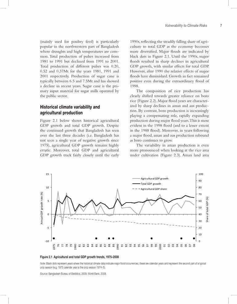
Figure 2.1 below shows historical agricultural GDP growth and total GDP growth. Despite the continued growth that Bangladesh has seen over the last three decades (i.e. Bangladesh has not seen a single year of negative growth since 1975), agricultural GDP growth remains highly erratic. Moreover, total GDP and agricultural GDP growth track fairly closely until the early
1990s, reflecting the steadily falling share of agri-culture to total GDP as the economy becomes more diversified. Major floods are indicated by black dots in Figure 2.1. Until the 1990s, major floods resulted in sharp declines in agricultural GDP growth, with similar effects for total GDP. However, after 1990 the relative effects of major floods have diminished. Growth in fact remained positive even during the extraordinary flood of 1998.
The composition of rice production has clearly shifted towards greater reliance on boro rice (Figure 2.2). Major flood years are character-ized by sharp declines in aman and aus produc-tion. By contrast, boro production is increasingly playing a compensating role, rapidly expanding production during major flood years. This is most evident in the 1998 flood (and to a lesser extent in the 1988 flood). Moreover, in years following a major flood, aman and aus production rebound as boro continues to grow.
The variability in aman production is even more pronounced when looking at the rice area under cultivation (Figure 2.3). Aman land area
Figure 2.1 Agricultural and total GDP growth trends, 1975–2008
Note: Black dots represent years where the historical climate data indicate major flood occurrences; these are calendar years and represent the second part of a typical crop season (e.g. 1975 calendar year is the crop season 1974–5).
Source: Bangladesh Bureau of Statistics, 2009; World Bank, 2009.
0
10
20
30
40
50
60
70
80
90
100
-10
-5
0
5
10
15
1975 76 77 78 79
1980 81 82 83 84 85 86 87 88 89
1990 91 92 93 94 95 96 97 98 99
2000 01 02 03 04 05 06 07 08
Shar
e of
tota
l GD
P (%
)
Ann
ual G
DP
grow
th r
ate
(%)
Agricultural GDP growth
Total GDP growth
Agricultural GDP share

8 Climate Change Risks and Food Security in Bangladesh
drops dramatically during major flood years, driving almost the entire decline in overall pro-duction.
Decomposing the historical aman rice pro-duction into land area and yield contributions shows that both contribute to the decline of aman production during major flood years (Fig-ure 2.4). However, in relative terms, the land area
declines dominate the yield changes. In contrast, yield improvements dominate the recovery years after floods. Observed yields for rice and wheat in Bangladesh from 1985 to 2000 have improved marginally over time (Figure 2.5).
Actual yields are much lower than the poten-tial yields (5–10kg/ha) observed at research plots under controlled field conditions (Sattar, 2000).
Figure 2.2 Historical trends in rice production quantities in Bangladesh, 1972–2006
Source: Bangladesh Bureau of Statistics, 2008c.
-25
-15
-5
5
15
25
35
45
1972
/73
73/7
4
74/7
5
75/7
6
76/7
7
77/7
8
78/7
9
79/8
0
80/8
1
81/8
2
82/8
3
83/8
4
84/8
5
85/8
6
86/8
7
87/8
8
88/8
9
89/9
0
90/9
1
91/9
2
92/9
3
93/9
4
94/9
5
95/9
6
96/9
7
97/9
8
98/9
9
99/0
0
2000
/01
01/0
2
02/0
3
03/0
4
04/0
5
05/0
6
Cont
ribu
�on
to a
nnua
l ric
e ar
ea g
row
th
(p
erce
ntag
e po
int)
Boro contribu�on
Aman contribu�on
Aus contribu�on
Total growth rate
Figure 2.3 Historical trends in land area under rice cultivation in Bangladesh, 1972–2006
Source: Bangladesh Bureau of Statistics, 2008c.
-10
-8
-6
-4
-2
0
2
4
6
8
1972
/73
73/7
4
74/7
5
75/7
6
76/7
7
77/7
8
78/7
9
79/8
0
80/8
1
81/8
2
82/8
3
83/8
4
84/8
5
85/8
6
86/8
7
87/8
8
88/8
9
89/9
0
90/9
1
91/9
2
92/9
3
93/9
4
94/9
5
95/9
6
96/9
7
97/9
8
98/9
9
99/0
0
2000
/01
01/0
2
02/0
3
03/0
4
04/0
5
05/0
6
Cont
ribu
�on
to a
nnua
l ric
e ar
ea g
row
th
(p
erce
ntag
e po
int)
Boro contribu�on
Aman contribu�on
Aus contribu�on
Total growth rate
Vulnerability to Climate Risks 9
A major factor for this can be attributed to the ability of existing varieties of rice to withstand the annual variations in climate conditions (unfa-vourable temperatures, floods and droughts) as well as pests and disease pressures which vary from season to season. In addition, low levels of
management play an important role including sub-optimal time of planting, use of poor qual-ity seed, unbalanced use of fertilizers and other inputs, and failure to control weeds. In addition, many farmers have not yet adopted modern rice varieties. Soil-related factors include reduced
Figure 2.4 Decomposition of historical aman rice production trends into land area and yield contributions, 1972–2006
Source: Bangladesh Bureau of Statistics, 2008c.
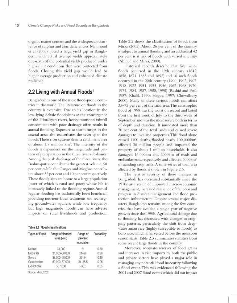
Figure 2.5 Observed yields for major staples (kg/ha)
Source: Bangladesh Bureau of Statistics, 2008c.
-20
-15
-10
-5
0
5
10
15
20
25
30
35
1972
/73
73/7
4
74/7
5
75/7
6
76/7
7
77/7
8
78/7
9
79/8
0
80/8
1
81/8
2
82/8
3
83/8
4
84/8
5
85/8
6
86/8
7
87/8
8
88/8
9
89/9
0
90/9
1
91/9
2
92/9
3
93/9
4
94/9
5
95/9
6
96/9
7
97/9
8
98/9
9
99/0
0
2000
/01
01/0
2
02/0
3
03/0
4
04/0
5
05/0
6
Cont
ribu
�on
to a
nnua
l Am
an r
ice
prod
uc�o
n gr
owth
(per
cent
age
poin
t)Produc�on
Yield contribu�on
Area contribu�on
Total growth rate
Observ
ed y
ield
s (
kg/h
a)
Total aus Total aman
Total boro Wheat
3500
3000
2500
2000
1500
1000
500
0
1985/86 1987/88 1989/90 1991/92 1993/94 1995/96 1997/98 1999/00
aman
10 Climate Change Risks and Food Security in Bangladesh
organic matter content and the widespread occur-rence of sulphur and zinc deficiencies. Mahmood et al (2003) noted a large yield gap in Bangla-desh, with actual average yields approximately one-sixth of the potential yields produced under high-input conditions that were protected from floods. Closing this yield gap would lead to higher average production and enhanced climate resilience.
2.2 Living with Annual Floods1
Bangladesh is one of the most flood-prone coun-tries in the world. The literature on floods in the country is extensive. Due to its location in the low-lying deltaic floodplains at the convergence of the Himalayan rivers, heavy monsoon rainfall concomitant with poor drainage often results in annual flooding. Exposure to storm surges in the coastal areas also exacerbates the severity of the floods. These river systems drain a catchment area of about 1.7 million km2. The intensity of the floods is dependent on the magnitude and pat-tern of precipitation in the three river sub-basins. Among the peak discharge of the three rivers, the Brahmaputra contributes the greatest volume, 58 per cent, while the Ganges and Meghna contrib-ute about 32 per cent and 10 per cent respectively. These floodplains are home to a large population (most of which is rural and poor) whose life is intricately linked to the flooding regime. Annual regular flooding has traditionally been beneficial, providing nutrient-laden sediments and recharg-ing groundwater aquifers; while low frequency but high magnitude floods can have adverse impacts on rural livelihoods and production.
Table 2.2 shows the classification of floods from Mirza (2002). About 26 per cent of the country is subject to annual flooding and an additional 42 per cent is at risk of floods with varied intensity (Ahmed and Mirza, 2000).
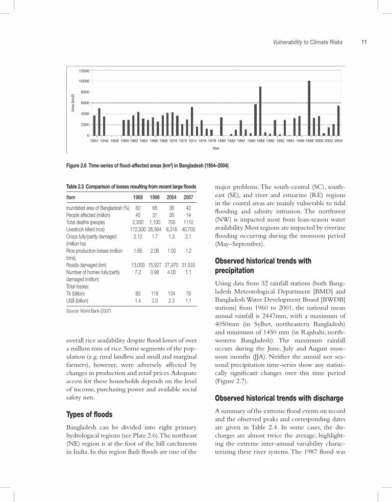
Historical records describe that five major floods occurred in the 19th century (1842, 1858, 1871, 1885 and 1892) and 16 such floods occurred in the 20th century (1900, 1902, 1907, 1918, 1922, 1954, 1955, 1956, 1962, 1968, 1970, 1974, 1984, 1987, 1988, 1998) (Rashid and Paul, 1987; Khalil, 1990; Haque, 1997; Chowdhury, 2000). Many of these serious floods can affect 35–75 per cent of the land area. The catastrophic flood of 1998 was the worst on record and lasted from the first week of July to the third week of September and was the most severe both in terms of depth and duration. It inundated more than 70 per cent of the total lands and caused severe damages to lives and properties. This flood alone caused 1100 deaths, flooded nearly 100,000km2, affected 30 million people and impacted the property of about 1 million households. It also damaged 16,000km and 6000km of roads and embankments, respectively, and affected 6000km2 of standing crop lands. A time-series of total area affected by floods is shown in Figure 2.6.
The relative severity of these disasters in Bangladesh has decreased substantially since the 1970s as a result of improved macro-economic management, increased resilience of the poor and progress in disaster management and flood pro-tection infrastructure. Despite several major dis-asters, Bangladesh remains among the few coun-tries that have avoided a single year of negative growth since the 1990s. Agricultural damage due to flooding has decreased with changes in crop-ping patterns, particularly the shift from deep-water aman rice (highly susceptible to floods) to boro rice, which is harvested before the monsoon season starts. Table 2.3 summarizes statistics from some recent large floods in the country.
Moreover, adequate reserves of food grains and increases in rice imports by both the public and private sectors have played a major role in managing any potential food insecurity following a flood event. This was evidenced following the 2004 and 2007 flood events which did not impact
Table 2.2 Flood classifications
Types of Flood Range of flooded area (km2)
Range of percent
inundation
Probability
Normal 31,000 21 0.50 Moderate 31,000–38,000 21–26 0.30 Severe 38,000–50,000 26–34 0.10 Catastrophic 50,000–57,000 34–38.5 0.05 Exceptional >57,000 >38.5 0.05
Source: Mirza, 2002.
Vulnerability to Climate Risks 11
overall rice availability despite flood losses of over a million tons of rice. Some segments of the pop-ulation (e.g. rural landless and small and marginal farmers), however, were adversely affected by changes in production and retail prices. Adequate access for these households depends on the level of income, purchasing power and available social safety nets.
Types of floods
Bangladesh can be divided into eight primary hydrological regions (see Plate 2.6). The northeast (NE) region is at the foot of the hill catchments in India. In this region flash floods are one of the
major problems. The south-central (SC), south-east (SE), and river and estuarine (RE) regions in the coastal areas are mainly vulnerable to tidal flooding and salinity intrusion. The northwest (NW) is impacted most from lean-season water availability. Most regions are impacted by riverine flooding occurring during the monsoon period (May–September).
Observed historical trends with precipitation
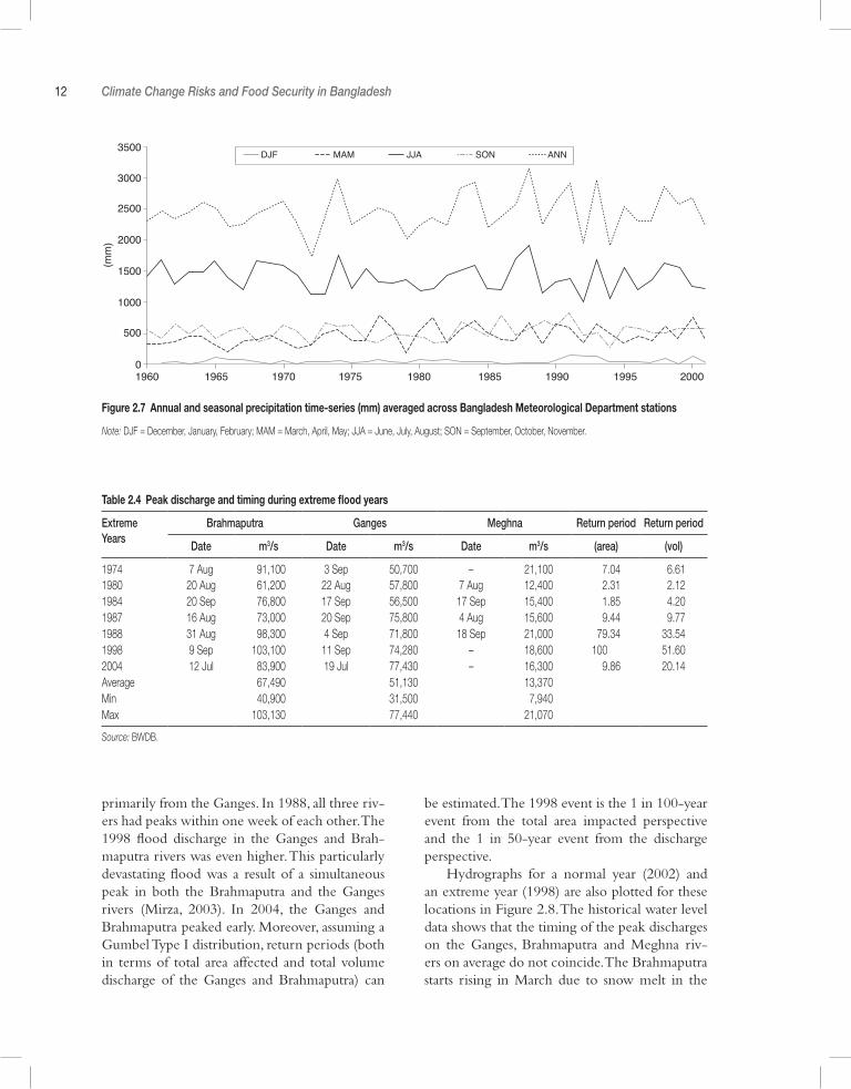
Using data from 32 rainfall stations (both Bang-ladesh Meteorological Department [BMD] and Bangladesh Water Development Board [BWDB] stations) from 1960 to 2001, the national mean annual rainfall is 2447mm, with a maximum of 4050mm (in Sylhet, northeastern Bangladesh) and minimum of 1450 mm (in Rajshahi, north-western Bangladesh). The maximum rainfall occurs during the June, July and August mon-soon months (JJA). Neither the annual nor sea-sonal precipitation time-series show any statisti-cally significant changes over this time period (Figure 2.7).
Observed historical trends with discharge
A summary of the extreme flood events on record and the observed peaks and corresponding dates are given in Table 2.4. In some cases, the dis-charges are almost twice the average, highlight-ing the extreme inter-annual variability charac-terizing these river systems. The 1987 flood was
Figure 2.6 Time-series of flood-affected areas (km2) in Bangladesh (1954–2004)
Table 2.3 Comparison of losses resulting from recent large floods
Item 1988 1998 2004 2007
Inundated area of Bangladesh (%) 60 68 38 42People affected (million) 45 31 36 14Total deaths (people) 2,300 1,100 750 1110Livestock killed (nos) 172,000 26,564 8,318 40,700Crops fully/partly damaged (million ha)
2.12 1.7 1.3 2.1
Rice production losses (million tons)
1.65 2.06 1.00 1.2
Roads damaged (km) 13,000 15,927 27,970 31,533Number of homes fully/partly damaged (million)
7.2 0.98 4.00 1.1
Total losses: Tk (billion)US$ (billion)
831.4
1182.0
1342.3
781.1
Source: World Bank (2007)
12000
10000
8000
6000
4000
2000
0
Are
a (k
m2)
1954 1956 1958 1960 1962 1964 1966 1968 1970 1972 1974 1976 1978 1980 1982 1984 1986 1988 1990 1992 1994 1996 1998 2000 2002 2004
Year
12 Climate Change Risks and Food Security in Bangladesh
primarily from the Ganges. In 1988, all three riv-ers had peaks within one week of each other. The 1998 flood discharge in the Ganges and Brah-maputra rivers was even higher. This particularly devastating flood was a result of a simultaneous peak in both the Brahmaputra and the Ganges rivers (Mirza, 2003). In 2004, the Ganges and Brahmaputra peaked early. Moreover, assuming a Gumbel Type I distribution, return periods (both in terms of total area affected and total volume discharge of the Ganges and Brahmaputra) can
be estimated. The 1998 event is the 1 in 100-year event from the total area impacted perspective and the 1 in 50-year event from the discharge perspective.
Hydrographs for a normal year (2002) and an extreme year (1998) are also plotted for these locations in Figure 2.8. The historical water level data shows that the timing of the peak discharges on the Ganges, Brahmaputra and Meghna riv-ers on average do not coincide. The Brahmaputra starts rising in March due to snow melt in the
Figure 2.7 Annual and seasonal precipitation time-series (mm) averaged across Bangladesh Meteorological Department stations
Note: DJF = December, January, February; MAM = March, April, May; JJA = June, July, August; SON = September, October, November.
Table 2.4 Peak discharge and timing during extreme flood years
ExtremeYears
Brahmaputra Ganges Meghna Return period Return period
Date m3/s Date m3/s Date m3/s (area) (vol)
1974 7 Aug 91,100 3 Sep 50,700 – 21,100 7.04 6.611980 20 Aug 61,200 22 Aug 57,800 7 Aug 12,400 2.31 2.121984 20 Sep 76,800 17 Sep 56,500 17 Sep 15,400 1.85 4.201987 16 Aug 73,000 20 Sep 75,800 4 Aug 15,600 9.44 9.771988 31 Aug 98,300 4 Sep 71,800 18 Sep 21,000 79.34 33.541998 9 Sep 103,100 11 Sep 74,280 – 18,600 100.34 51.602004 12 Jul 83,900 19 Jul 77,430 – 16,300 9.86 20.14Average 67,490 51,130 13,370 Min 40,900 31,500 7,940 Max 103,130 77,440 21,070
Source: BWDB.
1960 1965 1970 1975 1980 1985 1990 1995 2000
3500
3000
2500
2000
1500
1000
500
0
(mm)
JJA SON ANNMAMDJF
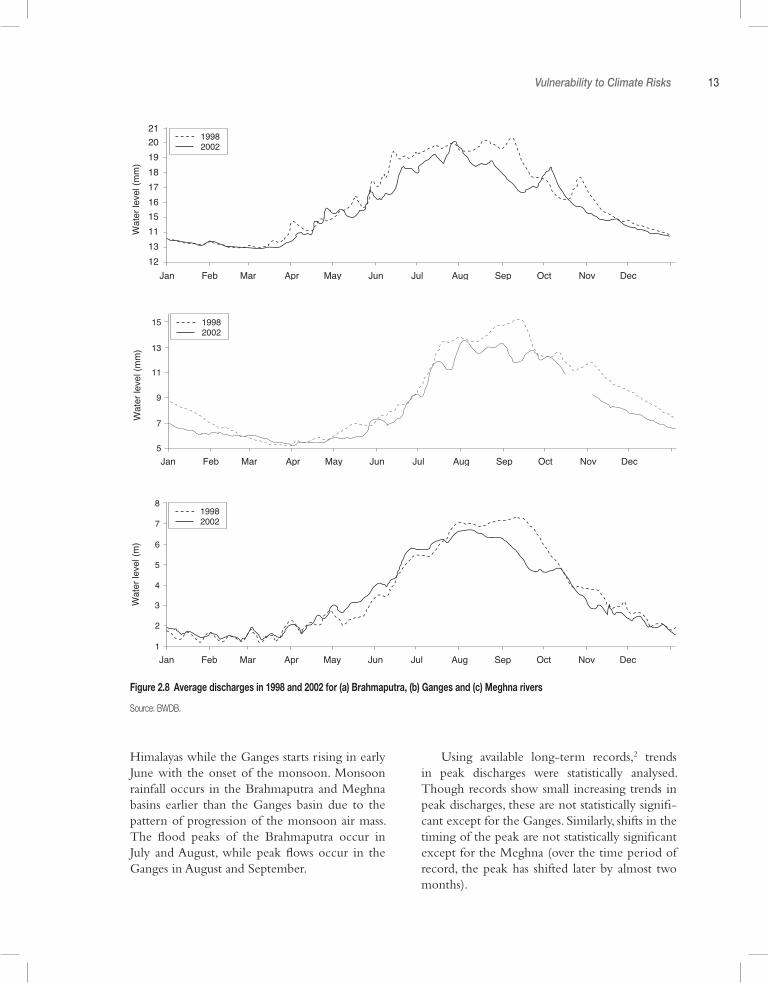
Vulnerability to Climate Risks 13
Himalayas while the Ganges starts rising in early June with the onset of the monsoon. Monsoon rainfall occurs in the Brahmaputra and Meghna basins earlier than the Ganges basin due to the pattern of progression of the monsoon air mass. The flood peaks of the Brahmaputra occur in July and August, while peak flows occur in the Ganges in August and September.
Using available long-term records,2 trends in peak discharges were statistically analysed. Though records show small increasing trends in peak discharges, these are not statistically signifi-cant except for the Ganges. Similarly, shifts in the timing of the peak are not statistically significant except for the Meghna (over the time period of record, the peak has shifted later by almost two months).
Figure 2.8 Average discharges in 1998 and 2002 for (a) Brahmaputra, (b) Ganges and (c) Meghna rivers
Source: BWDB.
21201918171615111312
Wat
er le
vel (
mm
)
Jan Feb Mar Apr May Jun Jul Aug Sep Oct Nov Dec
19982002
Wate
r le
vel (m
m)
Jan Feb Mar Apr May Jun Jul Aug Sep Oct Nov Dec
19982002
15
13
11
9
7
5
Wate
r le
vel (m
)
Jan Feb Mar Apr May Jun Jul Aug Sep Oct Nov Dec
19982002
6
7
8
5
4
3
2
1
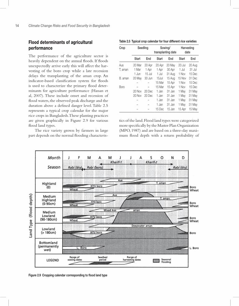
14 Climate Change Risks and Food Security in Bangladesh
Flood determinants of agricultural performance
The performance of the agriculture sector is heavily dependent on the annual floods. If floods unexpectedly arrive early this will affect the har-vesting of the boro crop while a late recession delays the transplanting of the aman crop. An indicator-based classification system for floods is used to characterize the primary flood deter-minants for agriculture performance (Hassan et al, 2007). These include onset and recession of flood waters, the observed peak discharge and the duration above a defined danger level. Table 2.5 represents a typical crop calendar for the major rice crops in Bangladesh. These planting practices are given graphically in Figure 2.9 for various flood land types.
The rice variety grown by farmers in large part depends on the normal flooding characteris-
Table 2.5 Typical crop calendar for four different rice varieties
Crop Seedling Sowing/transplanting date
Harvesting date
Start End Start End Start End
Aus 20 Mar 20 Apr 20 Apr 20 May 20 Jul 20 AugT. aman 1 Mar 1 Apr 1 Apr 30 Apr 1 Jul 31 Jul
1 Jun 15 Jul 1 Jul 31 Aug 1 Nov 15 DecB. aman 20 May 30 Jun 15Jul 15 Aug 15 Nov 31 Dec
– – 15 Mar 15 Apr 1 Nov 15 DecBoro – – 15 Mar 15 Apr 1 Nov 15 Dec
20 Nov 20 Dec 1 Jan 31 Jan 1 May 31 May20 Nov 20 Dec 1 Jan 31 Jan 1 May 31 May
– – 1 Jan 31 Jan 1 May 31 May– – 1 Jan 31 Jan 1 May 31 May– – 15 Dec 15 Jan 15 Apr 15 May
Figure 2.9 Cropping calendar corresponding to flood land type
tics of the land. Flood land types were categorized more specifically by the Master Plan Organization (MPO, 1987) and are based on a three-day maxi-mum flood depth with a return probability of
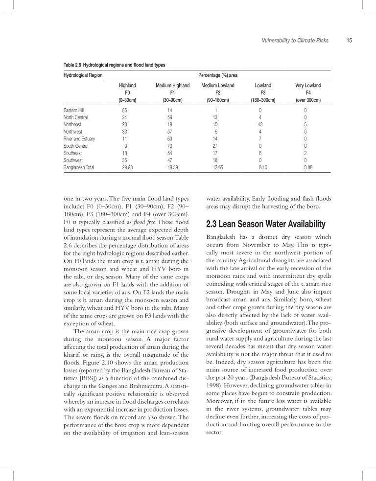
Vulnerability to Climate Risks 15
one in two years. The five main flood land types include: F0 (0–30cm), F1 (30–90cm), F2 (90–180cm), F3 (180–300cm) and F4 (over 300cm). F0 is typically classified as flood free. These flood land types represent the average expected depth of inundation during a normal flood season. Table 2.6 describes the percentage distribution of areas for the eight hydrologic regions described earlier. On F0 lands the main crop is t. aman during the monsoon season and wheat and HYV boro in the rabi, or dry, season. Many of the same crops are also grown on F1 lands with the addition of some local varieties of aus. On F2 lands the main crop is b. aman during the monsoon season and similarly, wheat and HYV boro in the rabi. Many of the same crops are grown on F3 lands with the exception of wheat.
The aman crop is the main rice crop grown during the monsoon season. A major factor affecting the total production of aman during the kharif, or rainy, is the overall magnitude of the floods. Figure 2.10 shows the aman production losses (reported by the Bangladesh Bureau of Sta-tistics [BBS]) as a function of the combined dis-charge in the Ganges and Brahmaputra. A statisti-cally significant positive relationship is observed whereby an increase in flood discharges correlates with an exponential increase in production losses. The severe floods on record are also shown. The performance of the boro crop is more dependent on the availability of irrigation and lean-season
water availability. Early flooding and flash floods areas may disrupt the harvesting of the boro.
2.3 Lean Season Water AvailabilityBangladesh has a distinct dry season which occurs from November to May. This is typi-cally most severe in the northwest portion of the country. Agricultural droughts are associated with the late arrival or the early recession of the monsoon rains and with intermittent dry spells coinciding with critical stages of the t. aman rice season. Droughts in May and June also impact broadcast aman and aus. Similarly, boro, wheat and other crops grown during the dry season are also directly affected by the lack of water avail-ability (both surface and groundwater). The pro-gressive development of groundwater for both rural water supply and agriculture during the last several decades has meant that dry season water availability is not the major threat that it used to be. Indeed, dry season agriculture has been the main source of increased food production over the past 20 years (Bangladesh Bureau of Statistics, 1998). However, declining groundwater tables in some places have begun to constrain production. Moreover, if in the future less water is available in the river systems, groundwater tables may decline even further, increasing the costs of pro-duction and limiting overall performance in the sector.
Table 2.6 Hydrological regions and flood land types
Hydrological Region Percentage (%) area
Highland Medium Highland Medium Lowland Lowland Very LowlandF0 F1 F2 F3 F4
(0–30cm) (30–90cm) (90–180cm) (180–300cm) (over 300cm)
Eastern Hill 85.98 14.98 1.98 0.10 0.10North Central 24.98 59.98 13.98 4.10 0.10Northeast 23.98 19.98 10.98 43.10 5.10Northwest 33.98 57.98 6.98 4.10 0.10River and Estuary 11.98 69.98 14.98 7.10 0.10South Central 0.98 73.98 27.98 0.10 0.10Southeast 18.98 54.98 17.98 8.10 2.10Southwest 35.98 47.98 18.98 0.10 0.10Bangladesh Total 29.98 48.39 12.65 8.10 0.88
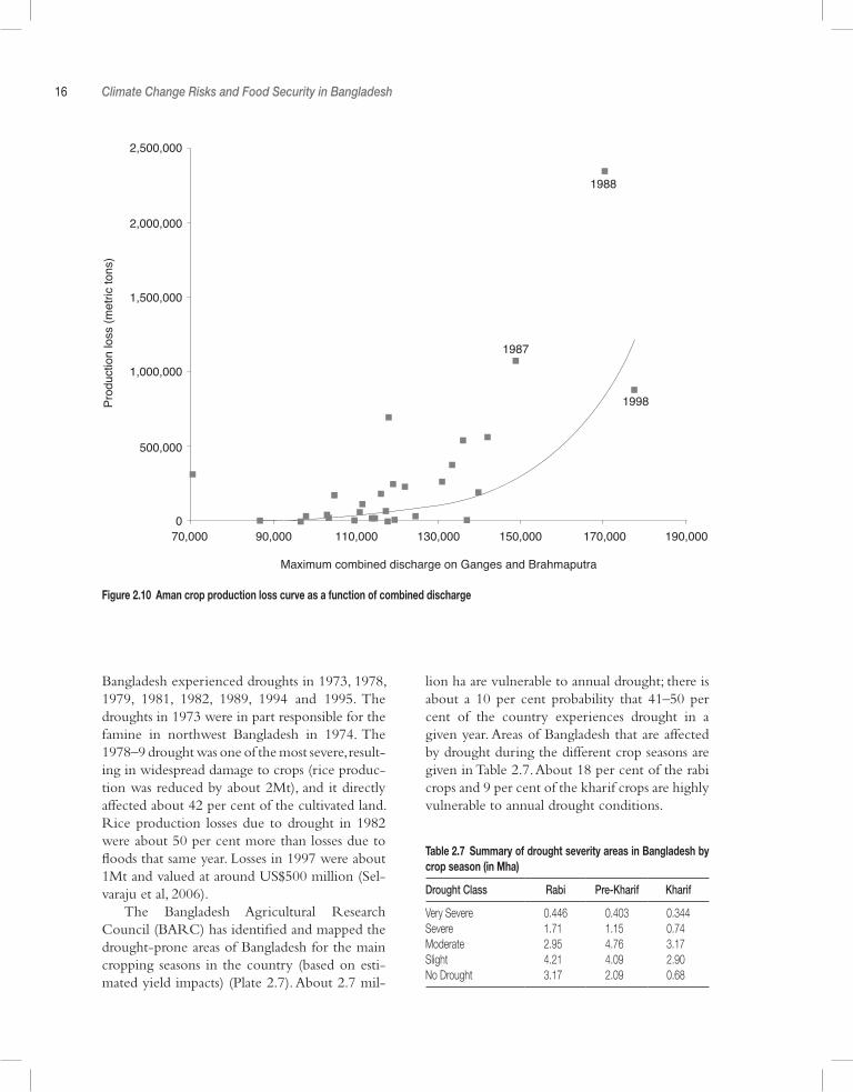
16 Climate Change Risks and Food Security in Bangladesh
Bangladesh experienced droughts in 1973, 1978, 1979, 1981, 1982, 1989, 1994 and 1995. The droughts in 1973 were in part responsible for the famine in northwest Bangladesh in 1974. The 1978–9 drought was one of the most severe, result-ing in widespread damage to crops (rice produc-tion was reduced by about 2Mt), and it directly affected about 42 per cent of the cultivated land. Rice production losses due to drought in 1982 were about 50 per cent more than losses due to floods that same year. Losses in 1997 were about 1Mt and valued at around US$500 million (Sel-varaju et al, 2006).
The Bangladesh Agricultural Research Council (BARC) has identified and mapped the drought-prone areas of Bangladesh for the main cropping seasons in the country (based on esti-mated yield impacts) (Plate 2.7). About 2.7 mil-
lion ha are vulnerable to annual drought; there is about a 10 per cent probability that 41–50 per cent of the country experiences drought in a given year. Areas of Bangladesh that are affected by drought during the different crop seasons are given in Table 2.7. About 18 per cent of the rabi crops and 9 per cent of the kharif crops are highly vulnerable to annual drought conditions.
Figure 2.10 Aman crop production loss curve as a function of combined discharge
Table 2.7 Summary of drought severity areas in Bangladesh by crop season (in Mha)
Drought Class Rabi Pre-Kharif Kharif
Very Severe 0.446 0.403 0.344Severe 1.716 1.156 0.746Moderate 2.956 4.766 3.176Slight 4.216 4.096 2.906No Drought 3.176 2.096 0.686
1987
1988
1998
70,0000
500,000
1,000,000
1,500,000
2,000,000
2,500,000
90,000 110,000 130,000 150,000 170,000 190,000
Prod
uctio
n lo
ss (m
etric
tons
)
Maximum combined discharge on Ganges and Brahmaputra
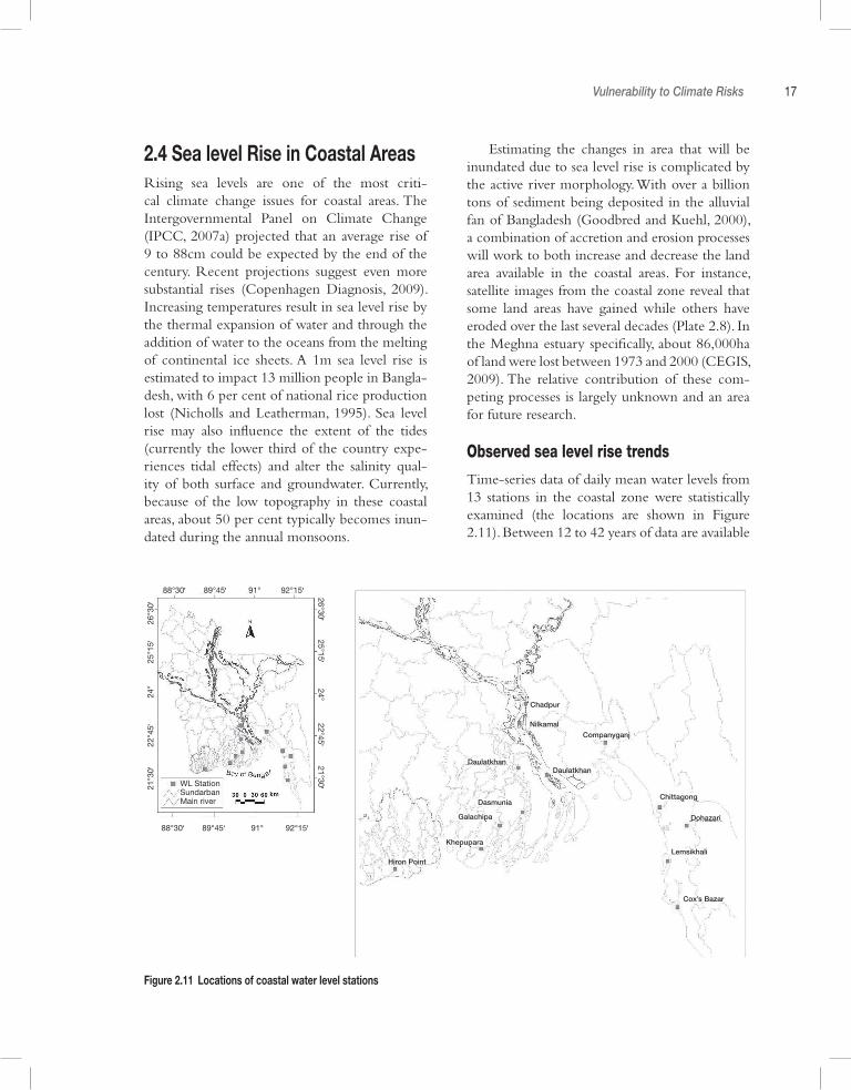
Vulnerability to Climate Risks 17
2.4 Sea level Rise in Coastal AreasRising sea levels are one of the most criti-cal climate change issues for coastal areas. The Intergovernmental Panel on Climate Change (IPCC, 2007a) projected that an average rise of 9 to 88cm could be expected by the end of the century. Recent projections suggest even more substantial rises (Copenhagen Diagnosis, 2009). Increasing temperatures result in sea level rise by the thermal expansion of water and through the addition of water to the oceans from the melting of continental ice sheets. A 1m sea level rise is estimated to impact 13 million people in Bangla-desh, with 6 per cent of national rice production lost (Nicholls and Leatherman, 1995). Sea level rise may also influence the extent of the tides (currently the lower third of the country expe-riences tidal effects) and alter the salinity qual-ity of both surface and groundwater. Currently, because of the low topography in these coastal areas, about 50 per cent typically becomes inun-dated during the annual monsoons.
Estimating the changes in area that will be inundated due to sea level rise is complicated by the active river morphology. With over a billion tons of sediment being deposited in the alluvial fan of Bangladesh (Goodbred and Kuehl, 2000), a combination of accretion and erosion processes will work to both increase and decrease the land area available in the coastal areas. For instance, satellite images from the coastal zone reveal that some land areas have gained while others have eroded over the last several decades (Plate 2.8). In the Meghna estuary specifically, about 86,000ha of land were lost between 1973 and 2000 (CEGIS, 2009). The relative contribution of these com-peting processes is largely unknown and an area for future research.
Observed sea level rise trends
Time-series data of daily mean water levels from 13 stations in the coastal zone were statistically examined (the locations are shown in Figure 2.11). Between 12 to 42 years of data are available
Figure 2.11 Locations of coastal water level stations
Chadpur
DaulatkhanDaulatkhan
Galachipa
Dasmunia
Nilkamal
Dohazari
Lemsikhali
Cox’s Bazar
Chittagong
Khepupara
Hiron Point
Companyganj
88°30' 89°45' 91° 92°15'
21°
30'
2
2°45
'
24°
25
°15'
26°3
0'
88°30' 89°45' 91° 92°15'
26°30'
25°15' 24°
22°45'
21°30'WL StationSundarbanMain river
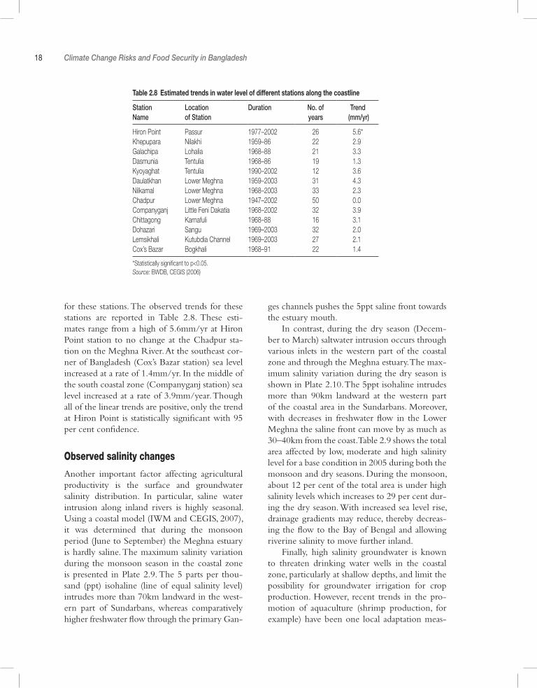
18 Climate Change Risks and Food Security in Bangladesh
for these stations. The observed trends for these stations are reported in Table 2.8. These esti-mates range from a high of 5.6mm/yr at Hiron Point station to no change at the Chadpur sta-tion on the Meghna River. At the southeast cor-ner of Bangladesh (Cox’s Bazar station) sea level increased at a rate of 1.4mm/yr. In the middle of the south coastal zone (Companyganj station) sea level increased at a rate of 3.9mm/year. Though all of the linear trends are positive, only the trend at Hiron Point is statistically significant with 95 per cent confidence.
Observed salinity changes
Another important factor affecting agricultural productivity is the surface and groundwater salinity distribution. In particular, saline water intrusion along inland rivers is highly seasonal. Using a coastal model (IWM and CEGIS, 2007), it was determined that during the monsoon period (June to September) the Meghna estuary is hardly saline. The maximum salinity variation during the monsoon season in the coastal zone is presented in Plate 2.9. The 5 parts per thou-sand (ppt) isohaline (line of equal salinity level) intrudes more than 70km landward in the west-ern part of Sundarbans, whereas comparatively higher freshwater flow through the primary Gan-
ges channels pushes the 5ppt saline front towards the estuary mouth.
In contrast, during the dry season (Decem-ber to March) saltwater intrusion occurs through various inlets in the western part of the coastal zone and through the Meghna estuary. The max-imum salinity variation during the dry season is shown in Plate 2.10. The 5ppt isohaline intrudes more than 90km landward at the western part of the coastal area in the Sundarbans. Moreover, with decreases in freshwater flow in the Lower Meghna the saline front can move by as much as 30–40km from the coast. Table 2.9 shows the total area affected by low, moderate and high salinity level for a base condition in 2005 during both the monsoon and dry seasons. During the monsoon, about 12 per cent of the total area is under high salinity levels which increases to 29 per cent dur-ing the dry season. With increased sea level rise, drainage gradients may reduce, thereby decreas-ing the flow to the Bay of Bengal and allowing riverine salinity to move further inland.
Finally, high salinity groundwater is known to threaten drinking water wells in the coastal zone, particularly at shallow depths, and limit the possibility for groundwater irrigation for crop production. However, recent trends in the pro-motion of aquaculture (shrimp production, for example) have been one local adaptation meas-
Table 2.8 Estimated trends in water level of different stations along the coastline
Station Name
Location of Station
Duration No. of years
Trend (mm/yr)
Hiron Point Passur 1977–2002 26 5.6*Khepupara Nilakhi 1959–86 22 2.9*Galachipa Lohalia 1968–88 21 3.3*Dasmunia Tentulia 1968–86 19 1.3*Kyoyaghat Tentulia 1990–2002 12 3.6*Daulatkhan Lower Meghna 1959–2003 31 4.3*Nilkamal Lower Meghna 1968–2003 33 2.3*Chadpur Lower Meghna 1947–2002 50 0.0*Companyganj Little Feni Dakatia 1968–2002 32 3.9*Chittagong Karnafuli 1968–88 16 3.1*Dohazari Sangu 1969–2003 32 2.0*Lemsikhali Kutubdia Channel 1969–2003 27 2.1*Cox’s Bazar Bogkhali 1968–91 22 1.4*
*Statistically significant to p<0.05.Source: BWDB, CEGIS (2006)

Vulnerability to Climate Risks 19
ure for coping with saline surface and groundwa-ter. Deeper in the aquifer, at depths greater than 150m, groundwater is typically fresh, thus much of the groundwater used for drinking water sup-ply is drawn from these depths.
2.5 Regional Hydrology IssuesDue to its location at the confluence of the Gan-ges, Brahmaputra and Meghna rivers, a discussion of water resources in Bangladesh is not complete without consideration of the broader basin region of which it is a part (Figure 2.12). This invariably requires an examination of its relationship with its neighbours: India, Nepal, China, Bhutan and Myanmar. The hydro-climatic, demographic and socio-economic features that characterize the patterns of water utilization in these shared river basins in the region have important implica-tions for the overall quantity and quality of water resources available as well as for the relationships among and within riparian states.
The annual rate of population growth in each of these riparian nations is similar (about 1 per cent). Population increases throughout the basins, coupled with increased demand for agri-cultural production, municipal and industrial requirements, environmental flows and energy production, will contribute to increasing water demands. Upstream changes in water demand in the Ganges alone, which currently has a popula-tion of 500 million people and contains 82 large cities with populations of 100,000 people or more, will play a significant role in the provision and timing of water downstream in Bangladesh. Moreover, changes in the quality of the water that is returned to the system (e.g. irrigation and
municipal return flows) may place further pres-sures on the gap between supply and demand for Bangladesh.
Balancing these future demands against future supplies may increasingly become difficult. Of particular importance to the region are the greater Himalayas where ten of the largest rivers in Asia begin (Amu Darya, Brahmaputra, Gan-ges, Indus, Irawaddy, Mekong, Salween, Tarim, Yangtze and Yellow rivers). These river basins are inhabited by over 1.3 billion people. Thus, this water ‘tower’ is critical to the overall economy of the region. With rising temperatures, it is reported that a rapid reduction in glaciers is being observed (Dyurgerov and Meier, 2005). With this glacier retreat, the rivers that originate at the glacier termini and derive significant volume of annual flow from glacier melt may experience profound downstream impacts on water resources. How-ever, much more research is needed to determine the exact balance among glacier melt, snow and precipitation contributions to the available dis-charge in each of these rivers. Current estimates of glacier melt contribution to runoff are around 9 and 12 per cent for the Ganges and Brahmapu-tra respectively (Jianchu et al, 2007).
A major limitation currently is that these mountain systems are poorly understood. The Himalayas are characterized by a complex three-dimensional mosaic of meteorological and hydro-logical environments, ranging from tropical rain-forests to alpine deserts, covering an altitudinal range of more than 8000m. Essential climate and hydrologic data is not readily available. The lack of a basic understanding of runoff sources and timing in these rivers makes it difficult to resolve questions relating to the overall water budget.
Table 2.9 Area affected by low, moderate and high salinity level (in 2005)
Season Total area (km2) Area affected (km2) Percentage of area affected (%)
Dry Season(Dec–Mar)
0–1 ppt Low 25,625 541–5 ppt Moderate 7808 17>5 ppt High 13,712 29
Monsoon Season (Jun–Sep) 0–1 ppt Low 37,455 791–5 ppt Moderate 4063 9>5 ppt High 5707 12
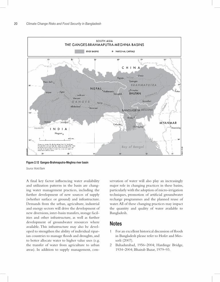
20 Climate Change Risks and Food Security in Bangladesh
Figure 2.12 Ganges-Brahmaputra-Meghna river basin
Source: World Bank
A final key factor influencing water availability and utilization patterns in the basin are chang-ing water management practices, including the further development of new sources of supply (whether surface or ground) and infrastructure. Demands from the urban, agriculture, industrial and energy sectors will drive the development of new diversions, inter-basin transfers, storage facil-ities and other infrastructure, as well as further development of groundwater resources where available. This infrastructure may also be devel-oped to strengthen the ability of individual ripar-ian countries to manage floods and droughts, and to better allocate water to higher value uses (e.g. the transfer of water from agriculture to urban areas). In addition to supply management, con-
servation of water will also play an increasingly major role in changing practices in these basins, particularly with the adoption of micro-irrigation techniques, promotion of artificial groundwater recharge programmes and the planned reuse of water. All of these changing practices may impact the quantity and quality of water available to Bangladesh.
Notes1 For an excellent historical discussion of floods
in Bangladesh please refer to Hofer and Mes-serli (2007).
2 Bahadurabad, 1956–2004; Hardinge Bridge, 1934–2004; Bhairab Bazar, 1979–93.
3
Future Climate Scenarios
Box 3.1 Key messages
• Projected temperature changes follow a positive trend for all months and seasons from the 2030s onwards. Median warming of 1.1°C, 1.6°C, and 2.6°C by the 2030s, 2050s and 2080s respectively is simulated from a range of plausible scenarios.
• Few months or seasons display clear drying or wetting trends in simulations of the 2030s. By the 2050s, annual and wet season precipitation is projected to trend towards increased precipitation. Only simulations for the dry season do not suggest an increase in precipitation. Across the model experiments, precipitation variations are large. Median annual precipitation increases of 1 per cent, 4 per cent and 7.4 per cent by the 2030s, 2050s and 2080s respectively are projected.
• Greater uncertainty (in terms of magnitude and direction) exists with future precipitation than future temperature.
• A trend toward a warmer and wetter future climate is projected to impact the agriculture sector, par-ticularly if the climate state goes beyond the variations found in the historical record. Projected future temperature changes significantly separate from the background temperature variations. Precipita-tion is subject to large existing inter-annual and intra-annual variations. Future precipitation projec-tions vary widely amongst models, with small median changes compared to historic variability.
• Using three scenarios of sea level rise (15cm, 27cm and 62cm), total flooded area in the coastal areas is projected to increase 6 per cent, 10 per cent and 20 per cent respectively.
Several climate change scenarios for Bangladesh have been published in recent years. Agrawala et al (2003) examined the performance of 17 glo-bal climate models (GCMs)1 over Bangladesh during the 20th century, then used several top-performing models to simulate future climate using the Intergovernmental Panel on Climate Change (IPCC) B2 emissions scenario (SRES, 2000).2 The resulting mean annual temperature changes were 1.4ºC by 2050 and 2.4ºC by 2100, with higher increases in the wintertime. Annual precipitation rose by 5.6 per cent by 2050 and 9.7 per cent by 2100, with indications of win-ter drying and summer rainfall increases. These projected seasonal changes are consistently found across many studies of the South Asian monsoon region.
Tanner et al (2007) followed a similar approach, identifying 10 out of 18 models from the IPCC Third Assessment Report (TAR) (IPCC, 2001) to project into the future using the IPCC A2 and B1 scenarios. Assessments were made for the 2020s and 2050s for Bangladesh and cover the entire GBM basin. Temperatures in 2050 were projected to increase by an average of 1.6ºC and 2.0ºC in the B1 and A2 scenarios respectively, with corresponding increases in rainfall of 4 per cent and 2 per cent. An additional analysis was conducted to generate probability distribution functions of climate change in Bangladesh using the climate sensitivities of 23 IPCC TAR models, assuming that each model was an equally likely representation of each future scenario. Again, pro-jected warming was more prevalent in winter
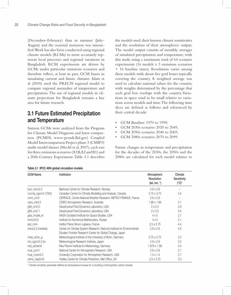
22 Climate Change Risks and Food Security in Bangladesh
(December–February) than in summer (July–August) and the seasonal monsoon was intensi-fied. Work has also been conducted using regional climate models (RCMs) to more accurately rep-resent local processes and regional variations in Bangladesh. RCM experiments are driven by GCMs under particular emissions scenarios and therefore reflect, at least in part, GCM biases in simulating current and future climates. Islam et al (2005) used the PRECIS regional model to compare regional anomalies of temperature and precipitation. The use of regional models in cli-mate projections for Bangladesh remains a key area for future research.
3.1 Future Estimated Precipitation and TemperatureSixteen GCMs were analyzed from the Program for Climate Model Diagnosis and Inter-compar-ison (PCMDI, www-pcmdi.llnl.gov) Coupled Model Intercomparison Project phase 3 (CMIP3) multi-model dataset (Meehl et al, 2007), each run for three emissions scenarios (A1B, A2 and B1) and a 20th-Century Experiment. Table 3.1 describes
the models used, their known climate sensitivities and the resolution of their atmospheric output. The model output consists of monthly averages of simulated precipitation and temperature, with this study using a maximum total of 64 scenario experiments (16 models x 3 emissions scenarios + 16 baseline states). Resolution varies among these models with about five grid boxes typically covering the country. A weighted average was used to calculate national values for the country, with weights determined by the percentage that each grid box overlaps with the country. Varia-tions in space tend to be small relative to varia-tions across models and time. The following time slices are defined as follows and referenced by their central decade:
• GCM Baseline: 1970 to 1999,• GCM 2030s scenario: 2020 to 2049,• GCM 2050s scenario: 2040 to 2069,• GCM 2080s scenario: 2070 to 2099.
Future changes in temperature and precipitation for the decades of the 2030s, the 2050s and the 2080s are calculated for each model relative to
Table 3.1 IPCC AR4 global circulation models
GCM Name Institution Atmospheric Resolution (lat, lon, °)
Climate Sensitivity
(°C)*
bccr_bcm2.0 Bjerknes Centre for Climate Research, Norway 2.8 x 2.8 –cccma_cgcm3.1(T63) Canadian Centre for Climate Modelling and Analysis, Canada 3.75 x 3.75 3.4cnrm_cm3 CERFACS, Centre National Weather Research, METEO-FRANCE, France 2.8 x 2.8 –csiro_mk3.0 CSIRO Atmospheric Research, Australia 1.88 x 1.88 3.1gfdl_cm2.0 Geophysical Fluid Dynamics Laboratory, USA 2 x 2.5 2.9gfdl_cm2.1 Geophysical Fluid Dynamics Laboratory, USA 2 x 2.5 3.4giss_model_er NASA Goddard Institute for Space Studies, USA 4 x 5 2.7inmcm3.0 Institute for Numerical Mathematics, Russia 4 x 5 2.1ipsl_cm4 Institut Pierre Simon Laplace, France 2.5 x 3.75 4.4miroc3.2 (medres) Center for Climate System Research; National Institute for Environmental
Studies; Frontier Research Center for Global Change, Japan2.8 x 2.8 4.0
miub_echo_g Meteorological Institute of the University of Bonn, Germany 3.75 x 3.75 3.2mri_cgcm2.3.2a Meteorological Research Institute, Japan 2.8 x 2.8 3.2mpi_echam5 Max Planck Institute for Meteorology, Germany 1.878 x 1.88 3.4ncar_pcm1 National Center for Atmospheric Research, USA 2.8 x 2.8 2.1ncar_ccsm3.0 University Corporation for Atmospheric Research, USA 1.4 x 1.4 2.7ukmo_hadcm3 Hadley Centre for Climate Prediction, Met Office, UK 2.5 x 3.75 3.3
* Climate sensitivity parameter defined as temperature increase for a doubling of atmospheric carbon dioxide.
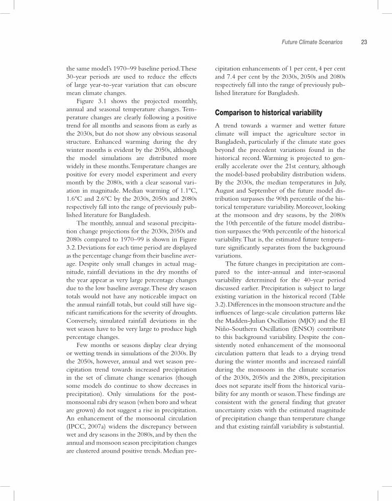
Future Climate Scenarios 23
the same model’s 1970–99 baseline period. These 30-year periods are used to reduce the effects of large year-to-year variation that can obscure mean climate changes.
Figure 3.1 shows the projected monthly, annual and seasonal temperature changes. Tem-perature changes are clearly following a positive trend for all months and seasons from as early as the 2030s, but do not show any obvious seasonal structure. Enhanced warming during the dry winter months is evident by the 2050s, although the model simulations are distributed more widely in these months. Temperature changes are positive for every model experiment and every month by the 2080s, with a clear seasonal vari-ation in magnitude. Median warming of 1.1ºC, 1.6ºC and 2.6ºC by the 2030s, 2050s and 2080s respectively fall into the range of previously pub-lished literature for Bangladesh.
The monthly, annual and seasonal precipita-tion change projections for the 2030s, 2050s and 2080s compared to 1970–99 is shown in Figure 3.2. Deviations for each time period are displayed as the percentage change from their baseline aver-age. Despite only small changes in actual mag-nitude, rainfall deviations in the dry months of the year appear as very large percentage changes due to the low baseline average. These dry season totals would not have any noticeable impact on the annual rainfall totals, but could still have sig-nificant ramifications for the severity of droughts. Conversely, simulated rainfall deviations in the wet season have to be very large to produce high percentage changes.
Few months or seasons display clear drying or wetting trends in simulations of the 2030s. By the 2050s, however, annual and wet season pre-cipitation trend towards increased precipitation in the set of climate change scenarios (though some models do continue to show decreases in precipitation). Only simulations for the post- monsoonal rabi dry season (when boro and wheat are grown) do not suggest a rise in precipitation. An enhancement of the monsoonal circulation (IPCC, 2007a) widens the discrepancy between wet and dry seasons in the 2080s, and by then the annual and monsoon season precipitation changes are clustered around positive trends. Median pre-
cipitation enhancements of 1 per cent, 4 per cent and 7.4 per cent by the 2030s, 2050s and 2080s respectively fall into the range of previously pub-lished literature for Bangladesh.
Comparison to historical variability
A trend towards a warmer and wetter future climate will impact the agriculture sector in Bangladesh, particularly if the climate state goes beyond the precedent variations found in the historical record. Warming is projected to gen-erally accelerate over the 21st century, although the model-based probability distribution widens. By the 2030s, the median temperatures in July, August and September of the future model dis-tribution surpasses the 90th percentile of the his-torical temperature variability. Moreover, looking at the monsoon and dry seasons, by the 2080s the 10th percentile of the future model distribu-tion surpasses the 90th percentile of the historical variability. That is, the estimated future tempera-ture significantly separates from the background variations.
The future changes in precipitation are com-pared to the inter-annual and inter-seasonal variability determined for the 40-year period discussed earlier. Precipitation is subject to large existing variation in the historical record (Table 3.2). Differences in the monsoon structure and the influences of large-scale circulation patterns like the Madden-Julian Oscillation (MJO) and the El Niño-Southern Oscillation (ENSO) contribute to this background variability. Despite the con-sistently noted enhancement of the monsoonal circulation pattern that leads to a drying trend during the winter months and increased rainfall during the monsoons in the climate scenarios of the 2030s, 2050s and the 2080s, precipitation does not separate itself from the historical varia-bility for any month or season. These findings are consistent with the general finding that greater uncertainty exists with the estimated magnitude of precipitation change than temperature change and that existing rainfall variability is substantial.
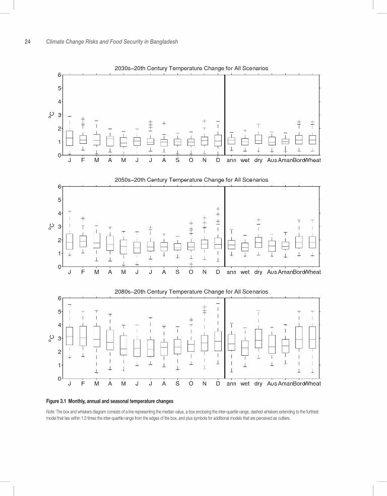
24 Climate Change Risks and Food Security in Bangladesh
Figure 3.1 Monthly, annual and seasonal temperature changes
Note: The box and whiskers diagram consists of a line representing the median value, a box enclosing the inter-quartile range, dashed whiskers extending to the furthest model that lies within 1.5 times the inter-quartile range from the edges of the box, and plus symbols for additional models that are perceived as outliers.
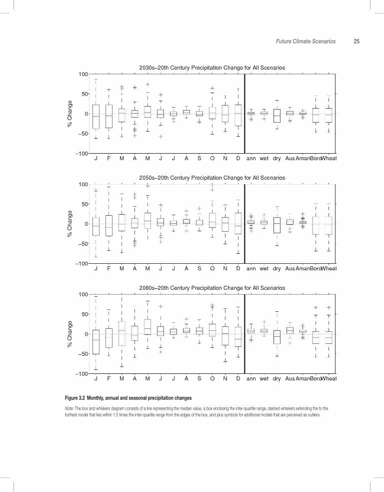
Future Climate Scenarios 25
Figure 3.2 Monthly, annual and seasonal precipitation changes
Note: The box and whiskers diagram consists of a line representing the median value, a box enclosing the inter-quartile range, dashed whiskers extending the to the furthest model that lies within 1.5 times the inter-quartile range from the edges of the box, and plus symbols for additional models that are perceived as outliers.
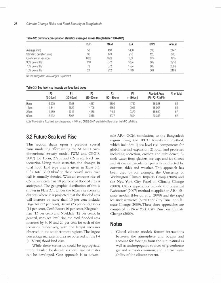
26 Climate Change Risks and Food Security in Bangladesh
3.2 Future Sea level RiseThis section draws upon a previous coastal zone modelling effort (using the MIKE21 two-dimensional estuary model, IWM and CEGIS, 2007) for 15cm, 27cm and 62cm sea level rise scenarios. Using these scenarios, the changes in total flood land type area is given in Table 3.3. Of a total 33,000km2 in these coastal areas, over half is annually flooded. With an extreme rise of 62cm, an increase in 10 per cent of flooded area is anticipated. The geographic distribution of this is shown in Plate 3.1. Under the 62cm rise scenario, districts where it is projected that the flooded area will increase by more than 10 per cent include: Bagerhat (22 per cent), Barisal (23 per cent), Bhola (14 per cent), Cox’s Bazar (10 per cent), Khagrach-hari (13 per cent) and Noakhali (12 per cent). In general, with sea level rise, the total flooded area increases by 6, 10 and 20 per cent for each of the scenarios respectively, with the largest increases observed in the southernmost regions. The largest percentage increases in area are observed for the F4 (+180cm) flood land class.
While these scenarios could be appropriate, more detailed local-scale sea level rise estimates can be developed. One approach is to downs-
cale AR4 GCM simulations to the Bangladesh region using the IPCC four-factor method, which includes: 1) sea level rise components for global thermal expansion; 2) local land processes including accretion, erosion and subsidence; 3) melt-water from glaciers, ice caps and ice sheets; and 4) coastal circulation patterns as affected by currents, tides and weather. This approach has been used by, for example, the University of Washington Climate Impacts Group (2008) and the New York City Panel on Climate Change (2009). Other approaches include the empirical Rahmstorf (2007) method as applied to AR4 cli-mate models (Horton et al, 2008) and the rapid ice-melt scenarios (New York City Panel on Cli-mate Change, 2009). These three approaches are compared in New York City Panel on Climate Change (2009).
Notes1 Global climate models feature interactions
between the atmosphere and oceans and account for forcings from the sun, natural as well as anthropogenic sources of greenhouse gas and aerosols emissions, and internal vari-ability of the climate system.
Table 3.2 Summary precipitation statistics averaged across Bangladesh (1960–2001)
DJF MAM JJA SON Annual
Average (mm) 53 460 1406 530 2447Standard deviation (mm) 36 149 216 125 306Coefficient of variation 68% 32% 15% 24% 12%90% percentile 118 672 1684 669 291075% percentile 72 572 1584 608 259310% percentile 21 312 1149 361 2199
Source: Bangladesh Meteorological Department.
Table 3.3 Sea level rise impacts on flood land types
F0(0–30cm)
F1(30–60cm)
F2(60–90cm)
F3(90–180cm)
F4(+180cm)
Flooded Area (F1+F2+F3+F4)
% of total
Base 15,920 4753 4517 5899 1759 16,928 5215cm 14,841 4522 4705 6765 2015 18,007 5527cm 14,189 4345 4488 7456 2370 18,659 5762cm 12,492 3967 3818 8977 3594 20,356 62
Note: Note that the flood land type classes used in IWM and CEGIS (2007) are slightly different than the MPO definitions.
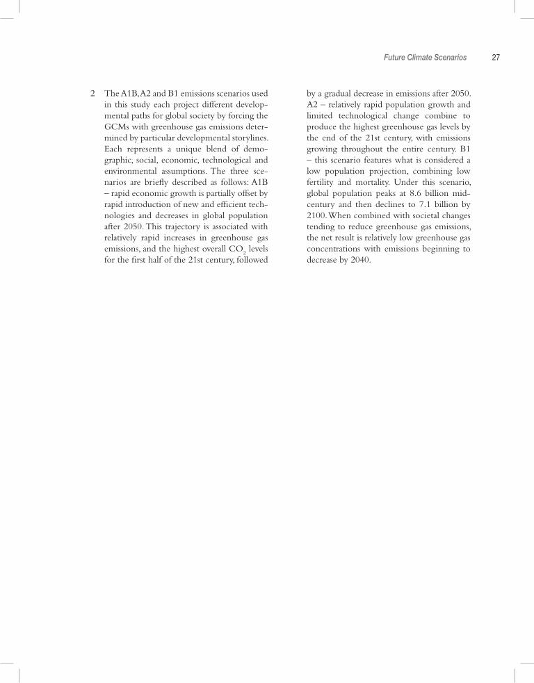
Future Climate Scenarios 27
2 The A1B, A2 and B1 emissions scenarios used in this study each project different develop-mental paths for global society by forcing the GCMs with greenhouse gas emissions deter-mined by particular developmental storylines. Each represents a unique blend of demo-graphic, social, economic, technological and environmental assumptions. The three sce-narios are briefly described as follows: A1B – rapid economic growth is partially offset by rapid introduction of new and efficient tech-nologies and decreases in global population after 2050. This trajectory is associated with relatively rapid increases in greenhouse gas emissions, and the highest overall CO
2 levels
for the first half of the 21st century, followed
by a gradual decrease in emissions after 2050. A2 – relatively rapid population growth and limited technological change combine to produce the highest greenhouse gas levels by the end of the 21st century, with emissions growing throughout the entire century. B1 – this scenario features what is considered a low population projection, combining low fertility and mortality. Under this scenario, global population peaks at 8.6 billion mid-century and then declines to 7.1 billion by 2100. When combined with societal changes tending to reduce greenhouse gas emissions, the net result is relatively low greenhouse gas concentrations with emissions beginning to decrease by 2040.

4
Future Flood Hydrology
Box 4.1 Key messages
• Primarily driven by increased monsoon precipitation in the GBM basin, models on average demon-strate increased flows in the three major rivers into Bangladesh (by as much as 20 per cent). Larger changes are anticipated by the 2050s compared to the 2030s. Larger changes are observed on average for the Ganges. The exact magnitude is dependent on the month.
• On average, models demonstrate that the flooded area increases in the future (over 10 per cent by the 2050s). This is primarily in the central part of the country at the confluence of the Ganges and Brahmaputra rivers and in the south. Flood area estimates separate from the background variations primarily in August and September at the height of the monsoon.
• Increases in yearly peak water levels are estimated for the northern sub-regions and decreases are estimated for the southern sub-regions. Not all estimated changes are statistically significant. More model experiments demonstrate changes that are significant by the 2050s than by the 2030s. Changes in the peak are in general less than 0.5m from the baseline.
• Across the sub-regions, most GCMs show earlier onset of the monsoon and a delay in the recession of flood waters.
Given the importance of flooding to overall agri-culture production, special effort was made to model the future flood hydrology under various climate change scenarios for the flood monsoon months (i.e. May–September). To do this, three sequential steps are taken: (1) a sub-set of cli-mate change scenarios are selected; (2) flows into Bangladesh are generated using a Ganges-Brah-maputra-Meghna (GBM) river basin model; and (3) hydrologic changes within the country are generated using a national river network model.
4.1 GBM Basin Model DevelopmentThe MIKE BASIN1 model was used for the GBM basin. Primary input data include topog-raphy, meteorology and hydrology information. River alignments for the GBM basin were deter-mined using available physical maps for India
and Nepal. For the topography of the basin, data from the Shuttle Radar Topography Mis-sion (SRTM) of the National Aeronautics and Space Administration (NASA) was used (Farr et al, 2007). GTOPO30, a global digital elevation model (DEM) from the United States Geological Survey (USGS), was used to fill in the gaps. The horizontal grid spacing for GTOPO30 is 30-arc seconds (approximately 1km) and for SRTM it is approximately 90m. This data was used to delin-eate sub-catchments. In total, the GBM basin model comprises 95 sub-catchments: 33 in the Brahmaputra basin, 55 in the Ganges basin and 7 in the Meghna basin.
Rainfall and evaporation data serve as bound-ary conditions for rain-fed sub-catchments. Irri-gation withdrawals and river management con-trols in upstream catchments were not considered in calibrating the model. Monthly temperature
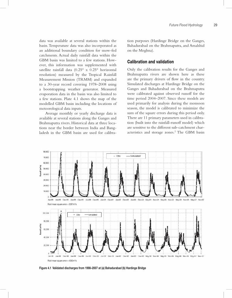
Future Flood Hydrology 29
data was available at several stations within the basin. Temperature data was also incorporated as an additional boundary condition for snow-fed catchments. Actual daily rainfall data within the GBM basin was limited to a few stations. How-ever, this information was supplemented with satellite rainfall data (0.25° x 0.25° horizontal resolution) measured by the Tropical Rainfall Measurement Mission (TRMM) and expanded to a 30-year record covering 1978–2008 using a bootstrapping weather generator. Measured evaporation data in the basin was also limited to a few stations. Plate 4.1 shows the map of the modelled GBM basin including the locations of meteorological data inputs.
Average monthly or yearly discharge data is available at several stations along the Ganges and Brahmaputra rivers. Historical data at three loca-tions near the border between India and Bang-ladesh in the GBM basin are used for calibra-
tion purposes (Hardinge Bridge on the Ganges, Bahadurabad on the Brahmaputra, and Amalshid on the Meghna).
Calibration and validation
Only the calibration results for the Ganges and Brahmaputra rivers are shown here as these are the primary drivers of flow in the country. Simulated discharges at Hardinge Bridge on the Ganges and Bahadurabad on the Brahmaputra were calibrated against observed runoff for the time period 2004–2007. Since these models are used primarily for analysis during the monsoon season, the model is calibrated to minimize the sum of the square errors during this period only. There are 11 primary parameters used in calibra-tion (built into the rainfall-runoff model) which are sensitive to the different sub-catchment char-acteristics and storage zones.2 The GBM basin
Figure 4.1 Validated discharges from 1998–2007 at (a) Bahadurabad (b) Hardinge Bridge
Root mean square error = 5287m3/s
Root mean square error = 4262m3/s
30 Climate Change Risks and Food Security in Bangladesh
model was then validated against TRMM data from 1998–2007 (shown in Figure 4.1). The model reasonably replicates the observed peaks.
4.2 National Hydrologic Super ModelInflows at the validated locations from the GBM basin model are used as boundary inflows into the national hydrologic model. This detailed model is the primary tool used by the government of Bangladesh to make annual flood forecasts and issue warnings. See Hopson and Webster (2007) for an application of this model using satellite imagery to improve the forecast from 3 days to 10 days. This model is combined with gridded precipitation and temperature data and predicts water levels and discharges throughout the coun-try. This model, which uses the MIKE 11 plat-form,3 predicts daily water levels and discharges throughout the country covering most of the major river networks (except for some parts in the coastal areas and eastern hills – see Plate 4.2a). A separate coastal model was used for the south-eastern part of the country. Plate 4.2a also shows the network of water levels and discharge points where time-series estimates are produced. With these daily water levels (at 3800 points), the tem-poral characteristics of the floods can be analysed. Moreover, monthly flood maps can be prepared using a three-dimensional Geographic Informa-tion Systems (GIS) tool to interpolate the flood surface while taking into account the presence of flood protection works (e.g. roads, embankments, polders). The area under different flood land type classes (as described in section 2.2) can then be calculated and compared to the baseline.
4.3 Approach to Modelling Future Flood ChangesRather than use the GCM future scenarios directly in these models, a ‘delta’ approach was taken to overcome four significant obstacles to climate scenarios generation: (1) GCM outputs may contain significant biases both in the base-line period and in the future period; (2) daily
output is required while the GCM output is typ-ically monthly; (3) the GCM spatial resolution reduces extreme events and misses sub-grid scale geographic variability; and (4) year-to-year vari-ability at a particular location in the GCM out-put tends to be underestimated due to simplified greenhouse forcing scenarios and coarse spatial resolution. Moreover, GCM contributions to the IPCC are designed to capture climatic changes averaged over a long period of time; not to simu-late particular events in the future. Therefore, the relevant information that may be taken from a GCM to generate climate scenarios is actually drawn from a comparison between a future pro-jection and a baseline period.
A monthly rainfall and temperature series, averaged over each 30-year time period, is deter-mined for the baseline and 2030s and 2050s sce-narios for a particular GCM. By comparing the baseline and future monthly averages, a ‘delta’ value for both rainfall and temperature can be calculated (i.e. percentage change is used for pre-cipitation and absolute change in degrees Celsius is used for temperature). Because the historical data captures differences between sub-regions and day-to-day and year-to-year variability that is not presented accurately in the GCM histori-cal output, this monthly change is then applied directly to the actual historical observed 30-year precipitation and temperature data.4 This approach removes much of the bias associated with each of the climate models, assuming that the bias is common to the historical and future periods. The sign and magnitude of remaining biases are unknown.
Selecting a sub-set of global climate models
Not all models could be tested in the flood sim-ulations because of resource limitations. Thus, a sub-set of GCMs was selected for the flood hydrology modelling. In using only a sub-set of models, care must be taken in interpreting the results. The reduction in the number of climate models results in a loss of information about the characteristics of future climate conditions and the statistical significance of those findings.
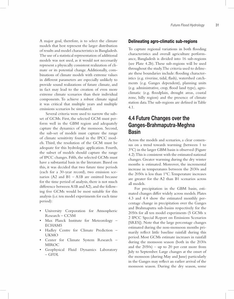
Future Flood Hydrology 31
A major goal, therefore, is to select the climate models that best represent the larger distribution of results and model characteristics in Bangladesh. The use of a statistical representation of additional models was not used, as it would not necessarily represent a physically consistent realization of cli-mate or its potential change. Additionally, com-binations of climate models with extreme values in different parameters are especially unlikely to provide sound realizations of future climate, and in fact may lead to the creation of even more extreme climate scenarios than their individual components. To achieve a robust climate signal it was critical that multiple years and multiple emissions scenarios be simulated.
Several criteria were used to narrow the sub-set of GCMs. First, the selected GCM must per-form well in the GBM region and adequately capture the dynamics of the monsoon. Second, the sub-set of models must capture the range of climate sensitivity found in the IPCC mod-els. Third, the resolution of the GCM must be adequate for this hydrologic application. Fourth, the subset of models should capture the range of IPCC changes. Fifth, the selected GCMs must have a substantial basis in the literature. Based on this, it was decided that two future time periods (each for a 30-year record), two emission sce-narios (A2 and B1 – A1B are omitted because for the time period of analysis, there is not much difference between A1B and A2), and the follow-ing five GCMs would be most suitable for this analysis (i.e. ten model experiments for each time period):
• University Corporation for Atmospheric Research – CCSM
• Max Planck Institute for Meteorology – ECHAM5
• Hadley Centre for Climate Prediction – UKMO
• Center for Climate System Research – MIROC
• Geophysical Fluid Dynamics Laboratory – GFDL
Delineating agro-climatic sub-regions
To capture regional variations in both flooding characteristics and overall agriculture perform-ance, Bangladesh is divided into 16 sub-regions (see Plate 4.2b). These sub-regions will be used throughout the study. The criteria used to deline-ate these boundaries include: flooding character-istics (e.g. riverine, tidal, flash), watershed catch-ments (e.g. Ganges dependent), planning units (e.g. administrative, crop, flood land type), agro-climatic (e.g. floodplain, drought areas, coastal zone, hilly region) and the presence of climate station data. The sub-regions are defined in Table 4.1.
4.4 Future Changes over the Ganges-Brahmaputra-Meghna BasinAcross the models and scenarios, a clear consen-sus on a trend towards warming (between 1 to 3°C) in the larger GBM basin is observed (Figure 4.2). This is consistent with the estimated national changes. Greater warming during the dry winter months is estimated. Moreover, the incremental increase in temperatures between the 2030s and the 2050s is less than 1°C. Temperature increases are greater for the A2 than B1 scenarios across all models.
For precipitation in the GBM basin, esti-mated changes differ widely across models. Plates 4.3 and 4.4 show the estimated monthly per-centage change in precipitation over the Ganges and Brahmaputra sub-basins respectively for the 2050s for all ten model experiments (5 GCMs x 2 IPCC Special Report on Emissions Scenarios [SRES]). Note that the large percentage changes estimated during the non-monsoon months pri-marily reflect little baseline rainfall during this period. Most GCMs estimate increases in rainfall during the monsoon season (both in the 2030s and the 2050s) – up to 20 per cent more from July to September. Large changes at the onset of the monsoon (during May and June) particularly in the Ganges may reflect an earlier arrival of the monsoon season. During the dry season, some
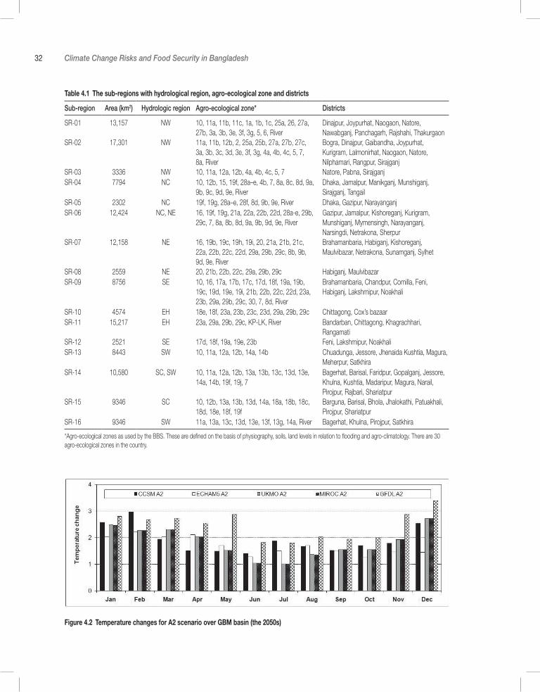
32 Climate Change Risks and Food Security in Bangladesh
Table 4.1 The sub-regions with hydrological region, agro-ecological zone and districts
Sub-region Area (km2) Hydrologic region Agro-ecological zone* Districts
SR-01 13,157 NW 10, 11a, 11b, 11c, 1a, 1b, 1c, 25a, 26, 27a, 27b, 3a, 3b, 3e, 3f, 3g, 5, 6, River
Dinajpur, Joypurhat, Naogaon, Natore, Nawabganj, Panchagarh, Rajshahi, Thakurgaon
SR-02 17,301 NW 11a, 11b, 12b, 2, 25a, 25b, 27a, 27b, 27c, 3a, 3b, 3c, 3d, 3e, 3f, 3g, 4a, 4b, 4c, 5, 7, 8a, River
Bogra, Dinajpur, Gaibandha, Joypurhat, Kurigram, Lalmonirhat, Naogaon, Natore, Nilphamari, Rangpur, Sirajganj
SR-03 3336 NW 10, 11a, 12a, 12b, 4a, 4b, 4c, 5, 7 Natore, Pabna, SirajganjSR-04 7794 NC 10, 12b, 15, 19f, 28a–e, 4b, 7, 8a, 8c, 8d, 9a,
9b, 9c, 9d, 9e, RiverDhaka, Jamalpur, Manikganj, Munshiganj, Sirajganj, Tangail
SR-05 2302 NC 19f, 19g, 28a–e, 28f, 8d, 9b, 9e, River Dhaka, Gazipur, NarayanganjSR-06 12,424 NC, NE 16, 19f, 19g, 21a, 22a, 22b, 22d, 28a-e, 29b,
29c, 7, 8a, 8b, 8d, 9a, 9b, 9d, 9e, RiverGazipur, Jamalpur, Kishoreganj, Kurigram, Munshiganj, Mymensingh, Narayanganj, Narsingdi, Netrakona, Sherpur
SR-07 12,158 NE 16, 19b, 19c, 19h, 19i, 20, 21a, 21b, 21c, 22a, 22b, 22c, 22d, 29a, 29b, 29c, 8b, 9b, 9d, 9e, River
Brahamanbaria, Habiganj, Kishoreganj, Maulvibazar, Netrakona, Sunamganj, Sylhet
SR-08 2559 NE 20, 21b, 22b, 22c, 29a, 29b, 29c Habiganj, MaulvibazarSR-09 8756 SE 10, 16, 17a, 17b, 17c, 17d, 18f, 19a, 19b,
19c, 19d, 19e, 19i, 21b, 22b, 22c, 22d, 23a, 23b, 29a, 29b, 29c, 30, 7, 8d, River
Brahamanbaria, Chandpur, Comilla, Feni, Habiganj, Lakshmipur, Noakhali
SR-10 4574 EH 18e, 18f, 23a, 23b, 23c, 23d, 29a, 29b, 29c Chittagong, Cox’s bazaarSR-11 15,217 EH 23a, 29a, 29b, 29c, KP-LK, River Bandarban, Chittagong, Khagrachhari,
RangamatiSR-12 2521 SE 17d, 18f, 19a, 19e, 23b Feni, Lakshmipur, NoakhaliSR-13 8443 SW 10, 11a, 12a, 12b, 14a, 14b Chuadunga, Jessore, Jhenaida Kushtia, Magura,
Meherpur, SatkhiraSR-14 10,580 SC, SW 10, 11a, 12a, 12b, 13a, 13b, 13c, 13d, 13e,
14a, 14b, 19f, 19j, 7Bagerhat, Barisal, Faridpur, Gopalganj, Jessore, Khulna, Kushtia, Madaripur, Magura, Narail, Pirojpur, Rajbari, Shariatpur
SR-15 9346 SC 10, 12b, 13a, 13b, 13d, 14a, 18a, 18b, 18c, 18d, 18e, 18f, 19f
Barguna, Barisal, Bhola, Jhalokathi, Patuakhali, Pirojpur, Shariatpur
SR-16 9346 SW 11a, 13a, 13c, 13d, 13e, 13f, 13g, 14a, River Bagerhat, Khulna, Pirojpur, Satkhira
*Agro-ecological zones as used by the BBS. These are defined on the basis of physiography, soils, land levels in relation to flooding and agro-climatology. There are 30 agro-ecological zones in the country.
Figure 4.2 Temperature changes for A2 scenario over GBM basin (the 2050s)
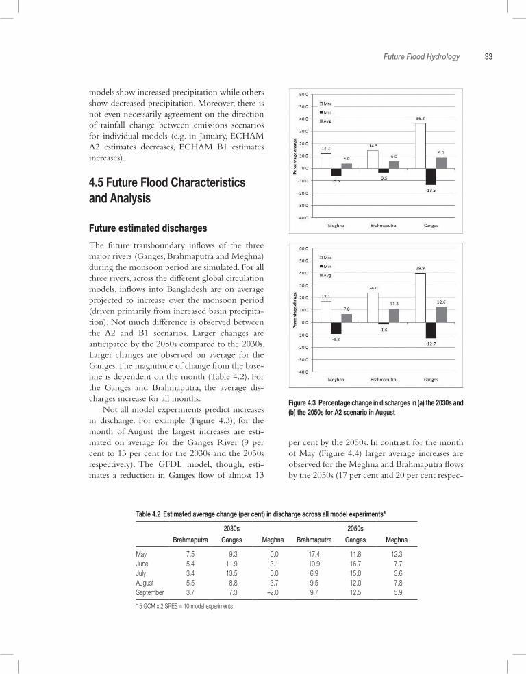
Future Flood Hydrology 33
models show increased precipitation while others show decreased precipitation. Moreover, there is not even necessarily agreement on the direction of rainfall change between emissions scenarios for individual models (e.g. in January, ECHAM A2 estimates decreases, ECHAM B1 estimates increases).
4.5 Future Flood Characteristics and Analysis
Future estimated discharges
The future transboundary inflows of the three major rivers (Ganges, Brahmaputra and Meghna) during the monsoon period are simulated. For all three rivers, across the different global circulation models, inflows into Bangladesh are on average projected to increase over the monsoon period (driven primarily from increased basin precipita-tion). Not much difference is observed between the A2 and B1 scenarios. Larger changes are anticipated by the 2050s compared to the 2030s. Larger changes are observed on average for the Ganges. The magnitude of change from the base-line is dependent on the month (Table 4.2). For the Ganges and Brahmaputra, the average dis-charges increase for all months.
Not all model experiments predict increases in discharge. For example (Figure 4.3), for the month of August the largest increases are esti-mated on average for the Ganges River (9 per cent to 13 per cent for the 2030s and the 2050s respectively). The GFDL model, though, esti-mates a reduction in Ganges flow of almost 13
Table 4.2 Estimated average change (per cent) in discharge across all model experiments*
2030s 2050s
Brahmaputra Ganges Meghna Brahmaputra Ganges Meghna
May 7.5 9.3 –0.0 17.4 11.8 12.3June 5.4 11.9 –3.1 10.9 16.7 7.7July 3.4 13.5 –0.0 6.9 15.0 3.6August 5.5 8.8 –3.7 9.5 12.0 7.8September 3.7 7.3 –2.0 9.7 12.5 5.9
* 5 GCM x 2 SRES = 10 model experiments
Figure 4.3 Percentage change in discharges in (a) the 2030s and (b) the 2050s for A2 scenario in August
per cent by the 2050s. In contrast, for the month of May (Figure 4.4) larger average increases are observed for the Meghna and Brahmaputra flows by the 2050s (17 per cent and 20 per cent respec-
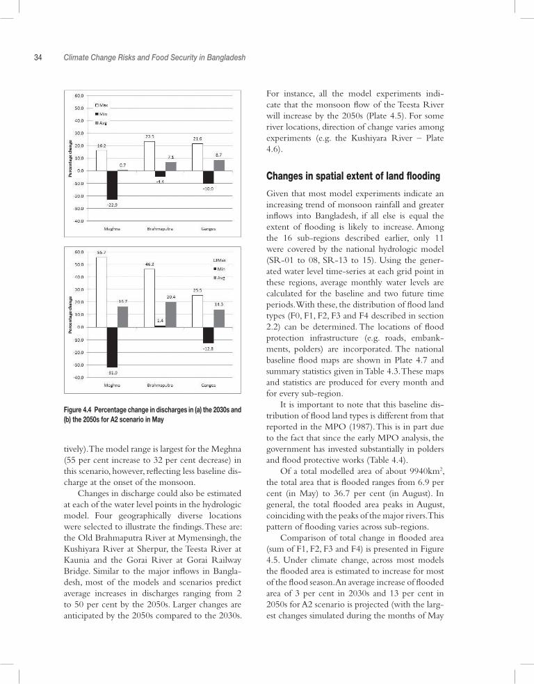
34 Climate Change Risks and Food Security in Bangladesh
tively). The model range is largest for the Meghna (55 per cent increase to 32 per cent decrease) in this scenario, however, reflecting less baseline dis-charge at the onset of the monsoon.
Changes in discharge could also be estimated at each of the water level points in the hydrologic model. Four geographically diverse locations were selected to illustrate the findings. These are: the Old Brahmaputra River at Mymensingh, the Kushiyara River at Sherpur, the Teesta River at Kaunia and the Gorai River at Gorai Railway Bridge. Similar to the major inflows in Bangla-desh, most of the models and scenarios predict average increases in discharges ranging from 2 to 50 per cent by the 2050s. Larger changes are anticipated by the 2050s compared to the 2030s.
For instance, all the model experiments indi-cate that the monsoon flow of the Teesta River will increase by the 2050s (Plate 4.5). For some river locations, direction of change varies among experiments (e.g. the Kushiyara River – Plate 4.6).
Changes in spatial extent of land flooding
Given that most model experiments indicate an increasing trend of monsoon rainfall and greater inflows into Bangladesh, if all else is equal the extent of flooding is likely to increase. Among the 16 sub-regions described earlier, only 11 were covered by the national hydrologic model (SR-01 to 08, SR-13 to 15). Using the gener-ated water level time-series at each grid point in these regions, average monthly water levels are calculated for the baseline and two future time periods. With these, the distribution of flood land types (F0, F1, F2, F3 and F4 described in section 2.2) can be determined. The locations of flood protection infrastructure (e.g. roads, embank-ments, polders) are incorporated. The national baseline flood maps are shown in Plate 4.7 and summary statistics given in Table 4.3. These maps and statistics are produced for every month and for every sub-region.
It is important to note that this baseline dis-tribution of flood land types is different from that reported in the MPO (1987). This is in part due to the fact that since the early MPO analysis, the government has invested substantially in polders and flood protective works (Table 4.4).
Of a total modelled area of about 9940km2, the total area that is flooded ranges from 6.9 per cent (in May) to 36.7 per cent (in August). In general, the total flooded area peaks in August, coinciding with the peaks of the major rivers. This pattern of flooding varies across sub-regions.
Comparison of total change in flooded area (sum of F1, F2, F3 and F4) is presented in Figure 4.5. Under climate change, across most models the flooded area is estimated to increase for most of the flood season. An average increase of flooded area of 3 per cent in 2030s and 13 per cent in 2050s for A2 scenario is projected (with the larg-est changes simulated during the months of May
Figure 4.4 Percentage change in discharges in (a) the 2030s and (b) the 2050s for A2 scenario in May
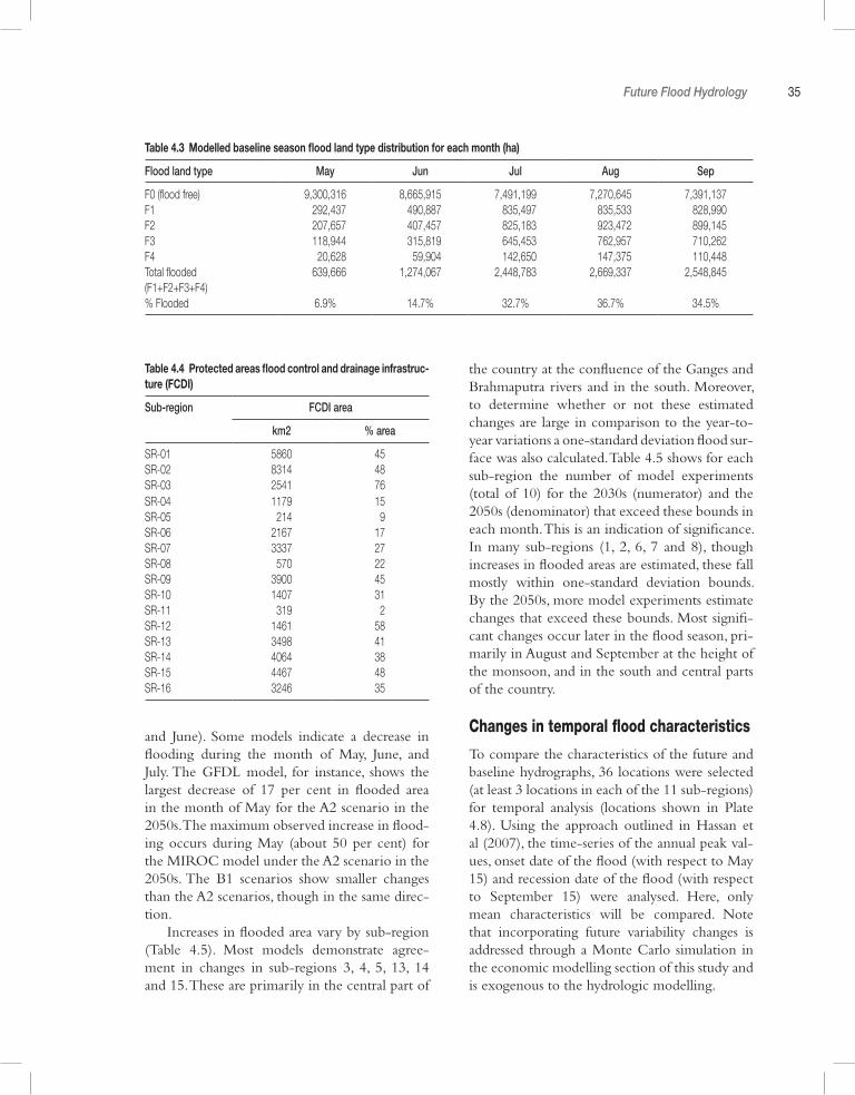
Future Flood Hydrology 35
and June). Some models indicate a decrease in flooding during the month of May, June, and July. The GFDL model, for instance, shows the largest decrease of 17 per cent in flooded area in the month of May for the A2 scenario in the 2050s. The maximum observed increase in flood-ing occurs during May (about 50 per cent) for the MIROC model under the A2 scenario in the 2050s. The B1 scenarios show smaller changes than the A2 scenarios, though in the same direc-tion.
Increases in flooded area vary by sub-region (Table 4.5). Most models demonstrate agree-ment in changes in sub-regions 3, 4, 5, 13, 14 and 15. These are primarily in the central part of
Table 4.3 Modelled baseline season flood land type distribution for each month (ha)
Flood land type May Jun Jul Aug Sep
F0 (flood free) 9,300,316 8,665,915 7,491,199 7,270,645 7,391,137F1 , 292,437 , 490,887 ,835,497 ,835,533 ,828,990F2 ,207,657 ,407,457 ,825,183 ,923,472 ,899,145F3 ,118,944 ,315,819 ,645,453 ,762,957 ,710,262F4 , 20,628 ,59,904 ,142,650 ,147,375 ,110,448Total flooded(F1+F2+F3+F4)
,639,666 1,274,067 2,448,783 2,669,337 2,548,845
% Flooded 6.9% 14.7% 32.7% 36.7% 34.5%
Table 4.4 Protected areas flood control and drainage infrastruc-ture (FCDI)
Sub-region FCDI area
km2 % area
SR-01 5860 45SR-02 8314 48SR-03 2541 76SR-04 1179 15SR-05 214 9SR-06 2167 17SR-07 3337 27SR-08 570 22SR-09 3900 45SR-10 1407 31SR-11 319 2SR-12 1461 58SR-13 3498 41SR-14 4064 38SR-15 4467 48SR-16 3246 35
the country at the confluence of the Ganges and Brahmaputra rivers and in the south. Moreover, to determine whether or not these estimated changes are large in comparison to the year-to-year variations a one-standard deviation flood sur-face was also calculated. Table 4.5 shows for each sub-region the number of model experiments (total of 10) for the 2030s (numerator) and the 2050s (denominator) that exceed these bounds in each month. This is an indication of significance. In many sub-regions (1, 2, 6, 7 and 8), though increases in flooded areas are estimated, these fall mostly within one-standard deviation bounds. By the 2050s, more model experiments estimate changes that exceed these bounds. Most signifi-cant changes occur later in the flood season, pri-marily in August and September at the height of the monsoon, and in the south and central parts of the country.
Changes in temporal flood characteristics
To compare the characteristics of the future and baseline hydrographs, 36 locations were selected (at least 3 locations in each of the 11 sub-regions) for temporal analysis (locations shown in Plate 4.8). Using the approach outlined in Hassan et al (2007), the time-series of the annual peak val-ues, onset date of the flood (with respect to May 15) and recession date of the flood (with respect to September 15) were analysed. Here, only mean characteristics will be compared. Note that incorporating future variability changes is addressed through a Monte Carlo simulation in the economic modelling section of this study and is exogenous to the hydrologic modelling.
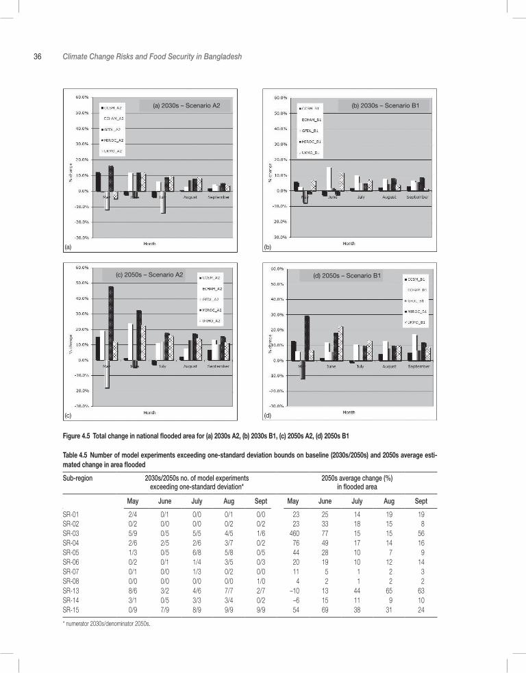
36 Climate Change Risks and Food Security in Bangladesh
Figure 4.5 Total change in national flooded area for (a) 2030s A2, (b) 2030s B1, (c) 2050s A2, (d) 2050s B1
Table 4.5 Number of model experiments exceeding one-standard deviation bounds on baseline (2030s/2050s) and 2050s average esti-mated change in area flooded
Sub-region 2030s/2050s no. of model experiments exceeding one-standard deviation*
2050s average change (%) in flooded area
May June July Aug Sept May June July Aug Sept
SR-01 2/4 0/1 0/0 0/1 0/0 – 23 25 14 19 19SR-02 0/2 0/0 0/0 0/2 0/2 –23 33 18 15 8SR-03 5/9 0/5 5/5 4/5 1/6 –460 77 15 15 56SR-04 2/6 2/5 2/6 3/7 0/2 –76 49 17 14 16SR-05 1/3 0/5 6/8 5/8 0/5 –44 28 10 7 9SR-06 0/2 0/1 1/4 3/5 0/3 –20 19 10 12 14SR-07 0/1 0/0 1/3 0/2 0/0 –11 5 1 2 3SR-08 0/0 0/0 0/0 0/0 1/0 4 2 1 2 2SR-13 8/6 3/2 4/6 7/7 2/7 –10 13 44 65 63SR-14 3/1 0/5 3/3 3/4 0/2 –6 15 11 9 10SR-15 0/9 7/9 8/9 9/9 9/9 – 54 69 38 31 24
* numerator 2030s/denominator 2050s.
(a) (b)
(c) (d)
(b) 2030s – Scenario B1(a) 2030s – Scenario A2
(c) 2050s – Scenario A2 (d) 2050s – Scenario B1

Future Flood Hydrology 37
Annual peak flowsTo estimate whether or not the peak flows are statistically changing under the climate change scenarios, the peak values at each of the 36 loca-tions are recorded for each year for the baseline and future time periods. Summary statistics (max, mean, min, standard deviation) are calculated. Hypothesis testing is performed to determine whether or not observed differences are statis-tically significant (null hypothesis that average peaks in the baseline and future time periods are not different). This is necessary because peak lev-els vary naturally from year to year. For instance, Figure 4.6 shows the observed peak water levels during the hydrologic baseline period (1978– 2008) at one location on the Jamuna in addition to the estimated peak water levels for the different model experiments for the 2030s. The baseline inter-annual variation is itself almost 0.5m (aver-age value of 11.6m). Thus, any observed change in average yearly peak levels must be considered in relation to this background variability.
Not all estimated changes in peak water lev-els are statistically significant. More model exper-iments demonstrate changes that are statistically significant (at the p < 0.01 level) by the 2050s. By the 2050s, many of the northern sub-regions (2–9) show statistically significant increases in the annual peak while many in the southwest (13–16) show decreases. Table 4.6 summarizes the observed changes in yearly peak levels, the number of model experiments that are statisti-
cally significant and the average change antici-pated for the 2050s. The greater the number of model experiments, the greater the agreement. Changes are in general less than 0.5m from the baseline. Estimated changes in sub-regions 3 and 15 are statistically the most robust. Estimated changes in sub-regions 1 and 9 are statistically the least robust.
Onset and recession timesAverage hydrographs were generated for each of the 36 locations for the baseline period and two future climate change futures to compare the
Figure 4.6 Yearly peak levels at Jamuna station for the baseline and model experiments (2030s)
Note: Solid line is historical baseline and dashed lines are all future model experiments.
Table 4.6 Peak water level summary for the 2050s
Sub-region No. model experiments* Average change (m)
SR-01 2 –0.47SR-02 10 –0.33SR-03 17 –0.27SR-04 6 –0.31SR-05 11 –0.28SR-06 8 –0.30SR-07 10 –0.43SR-08 6 –0.87SR-09 2 –0.27SR-13 10 –0.41SR-14 8 –0.19SR-15 22 –0.28SR-16 8 –0.28
*Number of model experiments where the estimated change is statistically different from the historical average peak level. Total number of model experiments is 30 (5 GCMs x 2 SRES x 3 stations per sub-region).
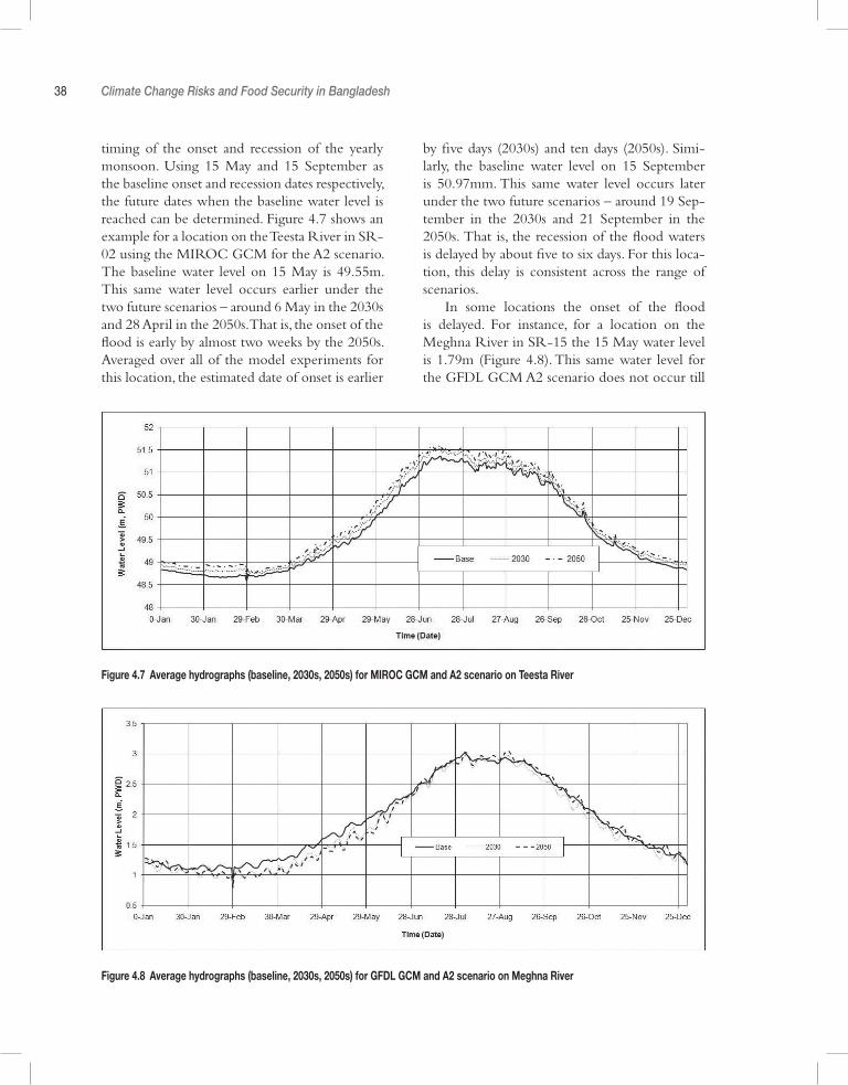
38 Climate Change Risks and Food Security in Bangladesh
timing of the onset and recession of the yearly monsoon. Using 15 May and 15 September as the baseline onset and recession dates respectively, the future dates when the baseline water level is reached can be determined. Figure 4.7 shows an example for a location on the Teesta River in SR-02 using the MIROC GCM for the A2 scenario. The baseline water level on 15 May is 49.55m. This same water level occurs earlier under the two future scenarios – around 6 May in the 2030s and 28 April in the 2050s. That is, the onset of the flood is early by almost two weeks by the 2050s. Averaged over all of the model experiments for this location, the estimated date of onset is earlier
by five days (2030s) and ten days (2050s). Simi-larly, the baseline water level on 15 September is 50.97mm. This same water level occurs later under the two future scenarios – around 19 Sep-tember in the 2030s and 21 September in the 2050s. That is, the recession of the flood waters is delayed by about five to six days. For this loca-tion, this delay is consistent across the range of scenarios.
In some locations the onset of the flood is delayed. For instance, for a location on the Meghna River in SR-15 the 15 May water level is 1.79m (Figure 4.8). This same water level for the GFDL GCM A2 scenario does not occur till
Figure 4.7 Average hydrographs (baseline, 2030s, 2050s) for MIROC GCM and A2 scenario on Teesta River
Figure 4.8 Average hydrographs (baseline, 2030s, 2050s) for GFDL GCM and A2 scenario on Meghna River
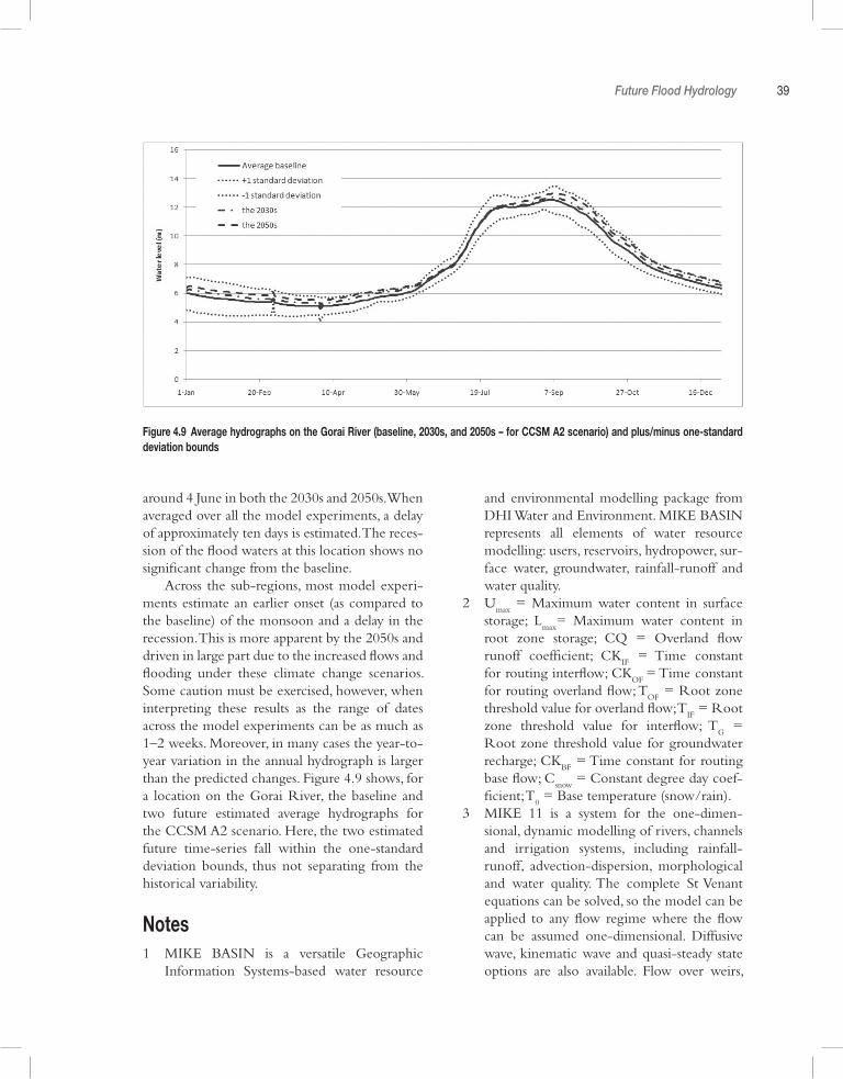
Future Flood Hydrology 39
Figure 4.9 Average hydrographs on the Gorai River (baseline, 2030s, and 2050s – for CCSM A2 scenario) and plus/minus one-standard deviation bounds
around 4 June in both the 2030s and 2050s. When averaged over all the model experiments, a delay of approximately ten days is estimated. The reces-sion of the flood waters at this location shows no significant change from the baseline.
Across the sub-regions, most model experi-ments estimate an earlier onset (as compared to the baseline) of the monsoon and a delay in the recession. This is more apparent by the 2050s and driven in large part due to the increased flows and flooding under these climate change scenarios. Some caution must be exercised, however, when interpreting these results as the range of dates across the model experiments can be as much as 1–2 weeks. Moreover, in many cases the year-to-year variation in the annual hydrograph is larger than the predicted changes. Figure 4.9 shows, for a location on the Gorai River, the baseline and two future estimated average hydrographs for the CCSM A2 scenario. Here, the two estimated future time-series fall within the one-standard deviation bounds, thus not separating from the historical variability.
Notes1 MIKE BASIN is a versatile Geographic
Information Systems-based water resource
and environmental modelling package from DHI Water and Environment. MIKE BASIN represents all elements of water resource modelling: users, reservoirs, hydropower, sur-face water, groundwater, rainfall-runoff and water quality.
2 Umax
= Maximum water content in surface storage; L
max= Maximum water content in
root zone storage; CQ = Overland flow runoff coefficient; CK
IF = Time constant
for routing interflow; CKOF
= Time constant for routing overland flow; T
OF = Root zone
threshold value for overland flow; TIF = Root
zone threshold value for interflow; TG =
Root zone threshold value for groundwater recharge; CK
BF = Time constant for routing
base flow; Csnow
= Constant degree day coef-ficient; T
0 = Base temperature (snow/rain).
3 MIKE 11 is a system for the one-dimen-sional, dynamic modelling of rivers, channels and irrigation systems, including rainfall-runoff, advection-dispersion, morphological and water quality. The complete St Venant equations can be solved, so the model can be applied to any flow regime where the flow can be assumed one-dimensional. Diffusive wave, kinematic wave and quasi-steady state options are also available. Flow over weirs,
40 Climate Change Risks and Food Security in Bangladesh
through culverts and user-defined structures, and over the flood plain can be simulated. Output from the hydrodynamic module can be routed to additional modules that simulate the transport of cohesive and non-cohesive sediment, dissolved oxygen, nutrients, heavy metals and eutrophication.
4 The baseline climate period (1979–99) differs slightly from the baseline hydrologic period (1978–2008) which introduces slightly higher baseline conditions for the ‘delta’ method. However, changes between 1999 and 2008 are the smallest of the 20th century.
5
Future Crop Performance
Box 5.1 Key messages
• Elevated CO2 concentrations are projected to have a substantial positive effect on crop yield for all crops and locations.
• Considering only temperature, precipitation and CO2 changes, aus and aman median production is projected to increase by 2 per cent and 4 per cent by the 2030s and the 2050s respectively. Wheat also increases, reaching a maximum of 4 per cent by 2050 before following a downward trend. These distributions range approximately +/– 2 per cent.
• Boro production is projected to decline under climate change scenarios, around 8 per cent by the 2080s. Changes for boro and wheat are conservative as it is assumed that farmers have uncon-strained access to irrigation.
• Shifts in the average floods are projected to reduce production of aus and aman by between 1 per cent and 4 per cent. The narrow model distribution of flood impacts projected by different GCMs suggest a robust change, although changes are small in comparison to year-to-year variability.
• The area lost to production due to sea level rise can be substantial. Maximum crop losses of nearly 40 per cent are projected by the 2080s for the south.
• Considering all climate impacts for the 2050s, the median of all rice crop projections show declining national production, with boro showing the largest median losses. However, for aus (–1.5 per cent) and aman (–0.6 per cent), the range of model experiments covers both gains and losses and does not statistically separate from zero. Most GCM projections estimate decline of boro production with a median loss of 3 per cent by the 2030s and 5 per cent by the 2050s. Wheat production increases up to the 2050s (3 per cent).
• In each sub-region, production losses are estimated for at least one crop. The production in the southern sub-regions is most vulnerable to climate change. For instance, average losses in SR-16 (containing Khulna) are –10 per cent for aus, aman and wheat, and –18 per cent for boro by the 2050s.
• The current large gap between actual and potential yields suggests substantial on-farm opportunities for growth and poverty reduction. Expanded availability of modern rice varieties, irrigation facilities, fertilizer use and labour could increase average yields at rates that could potentially more than offset the climate change impacts.
This section describes the use of a Decision Sup-port System for Agrotechnology Transfer model (DSSAT v4.5, Hoogenboom et al, 2003; Jones et al, 2003) to simulate agricultural yields under a range of climate change scenarios in Bangladesh.
The DSSAT model covers 16 sentinel locations in Bangladesh (to correspond to each sub-region described in the previous section) and focuses on yields of rice (primarily three seasons) and wheat. Simulations of changes in crop yield include
42 Climate Change Risks and Food Security in Bangladesh
impacts from climate only (CO2, temperature
and precipitation), floods and coastal inundation, both separately and in combination. For the cli-mate only simulations, probabilistic distributions of yield changes are generated across the set of global climate models, several emissions sce-narios (A1B, A2, and B) and future time slices (2030s, 2050s and 2080s). Together, these 16 loca-tions, 3 growing seasons, 3 emissions scenarios, 16 GCMs, 3 time-slices and 30-year periods for each simulation required the simulation of more than 200,000 individual DSSAT cropping seasons. The sensitivity of various individual cli-mate parameters was also extensively tested. The number of individual runs for the flood-damaged yields is significantly reduced as only a sub-set of model experiments are used (as described in section 4.3). The results of these simulations are reported here.
5.1 Development of the Baseline Period
CERES crop models
Crop simulations for this project utilized the Crop Environment Resource Synthesis (CERES) Rice and Wheat models, which are components of the DSSAT cropping systems model (Hoog-enboom et al, 2003). These dynamic biophysical crop models simulate plant growth on a per hec-tare basis, maintaining balances for water, carbon and nitrogen. CERES models have been applied previously in Bangladesh to model rice (Hussain, 1995; Mahmood et al, 2003) and rice-wheat sys-tems (Timsina and Humphreys, 2006a,b; Timsina et al, 1998). Studies examining climate change impacts on agricultural production in Bangladesh have also employed the CERES models (Karim et al, 1994; Hussain, 2006).
CERES models require information about the plant environment (weather and soils), cultivar genetics and agricultural management practices. Daily maximum and minimum temperatures, precipitation, carbon dioxide concentrations and solar radiation determine respiration and photo-synthesis rates, available water and evapotranspi-
ration rates. A soil profile provides information about available nutrients and root-zone moisture processes. Cultivar genetics determine the type of crop that is grown, including biophysical char-acteristics determining development and vulner-ability to environmental stresses. Management practices dictate the date, method and geometry of planting, as well as any applications of irriga-tion, fertilizer or chemicals.
As discussed in section 2.1, actual yields are much lower than the potential yields observed at experimental stations under controlled condi-tions. The model outputs for this study are poten-tial yields as simulated by the CERES models under recommended agricultural practices, and so validation of the potential yields is complex. Insects and rodents, which may severely damage infested areas, were not modeled. Thus, crops were assumed to be disease- and weed-free. Histori-cally, shortages or prohibitive costs of irrigation, fertilizer and labour reduce yields, while variation in management practices exists across the country. In addition, many farmers have not yet adopted modern rice varieties. For this study, as the main concern is to estimate the changes from the base-line, replicating the actual observed yields is of secondary importance. This, of course, assumes that crop response functions will be similar for high-input and low-input cropping systems.
The ability of the CERES models to accu-rately represent the agricultural impacts of anthro-pogenic climate change is hindered by consider-able uncertainty in the magnitude of CO
2 effects
(Easterling et al, 2007; Long et al, 2006; Tubiello et al, 2007a, b; Ainsworth et al, 2008; Hatfield et al 2008) and the location of temperature thresh-olds for crop damage. CO
2 is a primary element
of photosynthesis, and plants respond to elevated levels by increasing the rate of primary produc-tion. High CO
2 concentrations also increase root
densities and allow a plant to make more efficient gaseous transfers with its environment, collect-ing sufficient CO
2 in shorter periods of open leaf
stomata. This has the added effect of increasing water use efficiency in the plant as the duration that stomata are open is lessened and stomatal resistance is increased, reducing the loss of mois-ture to transpiration. Biophysical crop models,
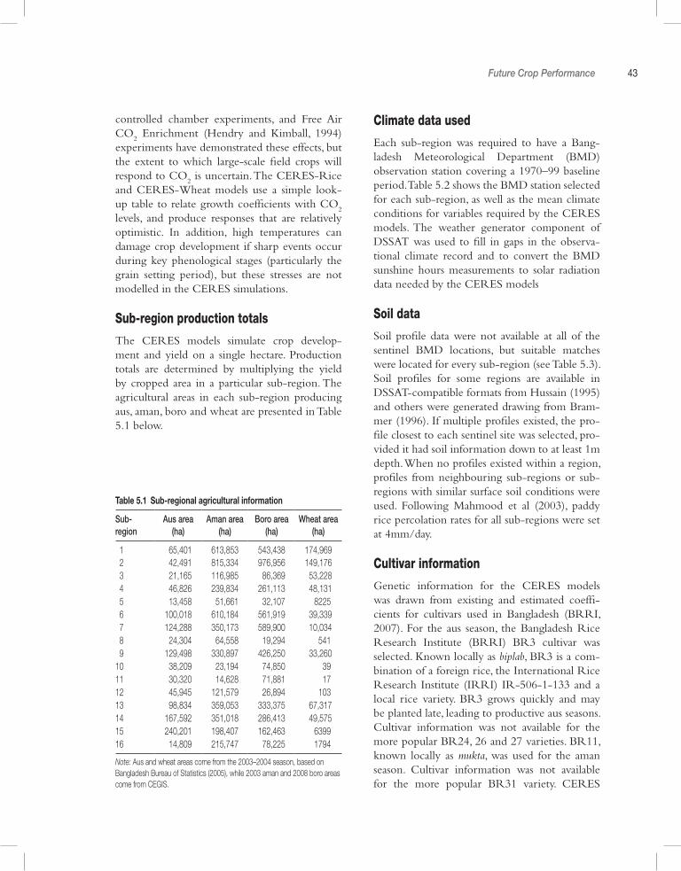
Future Crop Performance 43
controlled chamber experiments, and Free Air CO
2 Enrichment (Hendry and Kimball, 1994)
experiments have demonstrated these effects, but the extent to which large-scale field crops will respond to CO
2 is uncertain. The CERES-Rice
and CERES-Wheat models use a simple look-up table to relate growth coefficients with CO
2
levels, and produce responses that are relatively optimistic. In addition, high temperatures can damage crop development if sharp events occur during key phenological stages (particularly the grain setting period), but these stresses are not modelled in the CERES simulations.
Sub-region production totals
The CERES models simulate crop develop-ment and yield on a single hectare. Production totals are determined by multiplying the yield by cropped area in a particular sub-region. The agricultural areas in each sub-region producing aus, aman, boro and wheat are presented in Table 5.1 below.
Table 5.1 Sub-regional agricultural information
Sub-region
Aus area (ha)
Aman area (ha)
Boro area (ha)
Wheat area (ha)
1 65,401 613,853 543,438 174,969 2 42,491 815,334 976,956 149,176 3 21,165 116,985 86,369 53,228 4 46,826 239,834 261,113 48,131 5 13,458 51,661 32,107 8225 6 100,018 610,184 561,919 39,339 7 124,288 350,173 589,900 10,034 8 24,304 64,558 19,294 541 9 129,498 330,897 426,250 33,26010 38,209 23,194 74,850 3911 30,320 14,628 71,881 1712 45,945 121,579 26,894 10313 98,834 359,053 333,375 67,31714 167,592 351,018 286,413 49,57515 240,201 198,407 162,463 639916 14,809 215,747 78,225 1794
Note: Aus and wheat areas come from the 2003–2004 season, based on Bangladesh Bureau of Statistics (2005), while 2003 aman and 2008 boro areas come from CEGIS.
Climate data used
Each sub-region was required to have a Bang-ladesh Meteorological Department (BMD) observation station covering a 1970–99 baseline period. Table 5.2 shows the BMD station selected for each sub-region, as well as the mean climate conditions for variables required by the CERES models. The weather generator component of DSSAT was used to fill in gaps in the observa-tional climate record and to convert the BMD sunshine hours measurements to solar radiation data needed by the CERES models
Soil data
Soil profile data were not available at all of the sentinel BMD locations, but suitable matches were located for every sub-region (see Table 5.3). Soil profiles for some regions are available in DSSAT-compatible formats from Hussain (1995) and others were generated drawing from Bram-mer (1996). If multiple profiles existed, the pro-file closest to each sentinel site was selected, pro-vided it had soil information down to at least 1m depth. When no profiles existed within a region, profiles from neighbouring sub-regions or sub-regions with similar surface soil conditions were used. Following Mahmood et al (2003), paddy rice percolation rates for all sub-regions were set at 4mm/day.
Cultivar information
Genetic information for the CERES models was drawn from existing and estimated coeffi-cients for cultivars used in Bangladesh (BRRI, 2007). For the aus season, the Bangladesh Rice Research Institute (BRRI) BR3 cultivar was selected. Known locally as biplab, BR3 is a com-bination of a foreign rice, the International Rice Research Institute (IRRI) IR-506-1-133 and a local rice variety. BR3 grows quickly and may be planted late, leading to productive aus seasons. Cultivar information was not available for the more popular BR24, 26 and 27 varieties. BR11, known locally as mukta, was used for the aman season. Cultivar information was not available for the more popular BR31 variety. CERES

44 Climate Change Risks and Food Security in Bangladesh
Table 5.2 Climate information for each sub-region: the representative BMD station, its code and annual mean climate statistics during the 1970–99 baseline period
Sub-region
BMD Station Location BMD Station Code
Mean Tmax (°C)
Mean Tmin (°C)
Mean Rainfall (mm)
Mean Sunshine (MJ/m2/day)
1 Dinajpur 10,120 30.1 19.7 2003 16.9 2 Rangpur 10,208 29.7 19.9 2239 17.2 3 Ishwardi 10,910 31.7 20.3 1652 17.3 4 Tangail 41,909 30.3 20.8 1902 16.7 5 Dhaka 11,111 30.6 21.6 2148 17.6 6 Mymensingh 10,609 30.7 20.5 2255 16.4 7 Sylhet 10,705 29.6 20.2 4150 16.7 8 Srimangal 10,724 30.4 19.4 2421 17.7 9 Comilla 11,313 30.1 20.9 2054 17.210 Chittagong 11,921 30.2 21.6 2931 18.711 Rangamati 12,007 30.2 21.4 2532 17.712 Maijdee Court 11,809 29.8 21.6 3103 16.913 Jessore 11,407 31.4 20.9 1600 17.214 Faridpur 11,505 30.4 21.1 1967 17.215 Patuakhali 12,103 30.3 21.9 2704 15.616 Khulna 11,604 31.1 21.6 1812 17.4
Table 5.3 Soil profile information for each sub-region
Sub-region
Soil Location Soil Description Soil Type Soil Depth (cm)
Percolation Rate
(mm/day)
Initial Moisture
(mm)
Initial NO3 (kg N/ha)
Initial NH4 (kg N/ha)
1 Dinajpur Aeric Endoaquepts 130 4 243 44.7 4.112 Rangpur Aeric Endoaquepts 84 4 142 47.2 2.163 Jessore Aeric Endoaquepts 137 4 332 44.5 4.784 Karatia Silty Loam Aeric Endoaquepts 107 4 290 46.6 2.865 Ghatail Typic Dystrudepts 122 4 375 42.6 7.536 Phulpur Loam Aeric Endoaquepts 116 4 187 44.1 5.867 Biani Bazar Typic Dystrudepts 107 4 162 42.9 7.048 Srimangal Very fine sandy loam Udic Ustochrept 185 4 397 41.1 8.499 Shalpur Hyperthermic Typic
Endoaquept160 4 353 43.1 5.99
10 Chittagong Aeric Endoaquepts 216 4 378 39.6 9.7811 Srimangal Very fine sandy loam Udic Ustochrept 185 4 397 41.1 8.4912 Hatiya Silty Aeric Fluvaquent 165 4 543 41.6 8.0113 Jessore Aeric Endoaquepts 137 4 332 44.5 4.7814 Jessore Aeric Endoaquepts 137 4 332 44.5 4.7815 Satkhira Clay Loam Typic/Aeric Hapluquept 142 4 603 36.8 13.116 Satkhira Clay Loam Typic/Aeric Hapluquept 142 4 603 36.8 13.1
coefficients for BR11 transplanted aman and BR3 are distributed with DSSAT v4.5 (Hoog-enboom et al, 2003). BR29, introduced in 1994, was selected as a more current variety for the boro season, with genetic information provided by Dr Sk. Ghulam Hussain (at BARC). Kanchan,
the most common variety of wheat grown in Bangladesh, is not packaged with DSSAT v4.5. However, kanchan genetic coefficients exist for the CERES-Wheat model in DSSAT v3.0 and for the CropGro Wheat model in DSSAT v4.5. Using the coefficients from these model versions,
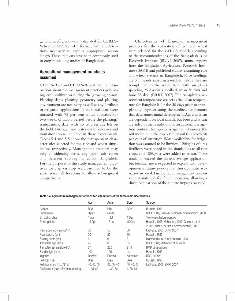
Future Crop Performance 45
genetic coefficients were estimated for CERES-Wheat in DSSAT v4.5 format, with modifica-tions necessary to capture appropriate season length. These cultivars have been commonly used in crop modelling studies of Bangladesh.
Agricultural management practices assumed
CERES-Rice and CERES-Wheat require infor-mation about the management practices govern-ing crop cultivation during the growing season. Planting dates, planting geometry and planting environment are necessary, as well as any fertilizer or irrigation applications. These simulations were initiated with 75 per cent initial moisture for two weeks of fallow period before the planting/transplanting date, with no crop residue left on the field. Nitrogen and water cycle processes and limitations were included in these experiments. Tables 5.4 and 5.5 show the management char-acteristics selected for the rice and wheat simu-lations respectively. Management practices may vary considerably across any given sub-region and between sub-regions across Bangladesh. For the purposes of this study, management prac-tices for a given crop were assumed to be the same across all locations to allow sub-regional comparisons.
Characteristics of farm-level management practices for the cultivation of rice and wheat were selected for the CERES models according to the recommendations of the Bangladesh Rice Research Institute (BRRI, 2007), annual reports from the Bangladesh Agricultural Research Insti-tute (BARI) and published studies examining rice and wheat systems in Bangladesh. Rice seedlings are commonly raised in a seedbed before they are transplanted to the wider field, with aus plants spending 25 days in a seedbed, aman 30 days and boro 35 days (BRRI, 2007). The transplant envi-ronment temperature was set as the mean tempera-ture for Bangladesh for the 30 days prior to trans-planting, approximating the seedbed temperature that determines initial development. Aus and aman are dependent on local rainfall, but boro and wheat are aided in the simulations by an automatic irriga-tion routine that applies irrigation whenever the soil moisture in the top 30cm of soil falls below 50 per cent of saturation. Water availability for irriga-tion was assumed to be limitless. 120kg/ha of urea fertilizers were added in the simulations to all rice crops, and 100kg/ha were added to wheat. These totals far exceed the current average application, but fertilizer use is expected to expand with devel-opment in future periods and thus optimistic sce-narios are used. Finally, these management options were maintained for future scenarios, allowing a direct comparison of the climate impacts on yield.
Table 5.4 Agriculture management options for simulations of the three main rice varieties
Aus Aman Boro Source
Cultivar BR3 BR11 BR29 Hussain, 1995Local name Biplab Mukta BRRI, 2007; Hussain, personal communication, 2008Simulation date 1 Apr 1 Jul 1 Dec Two weeks before plantingPlanting date 15 Apr 15 Jul 15 Dec Hussain, 1995; Mahmood, 1997; Gomosta et al,
2001; Hussain, personal communication, 2008Plant population (plants/m2) 50 50 50 Latif et al, 2005; BRRI, 2007Row spacing (cm) 20 20 20 Hussain, 1995Sowing depth (cm) 6 6 6 Mahmood et al, 2003; Hussain, 1995Transplant age (days) 25 30 35 BRRI, 2007; Mahmood et al, 2003Transplant temperature (ºC) 27 28.5 21.9 BMD observationsBund height (mm) 100 100 n/a Hussain, 1995Irrigation Rainfed Rainfed Automatic BBS, 2005bFertilizer type Urea Urea Urea Hussain, 1995Fertilizer amount (kg N/ha) 40, 40, 40 40, 40, 40 40, 40, 40 Latif et al, 2005; BRRI, 2007Applications (days after transplanting) 1, 30, 60 1, 30, 60 1, 30, 60
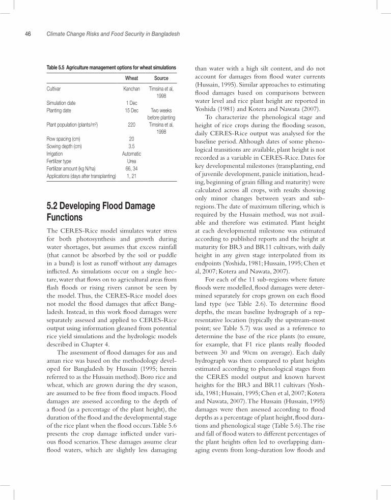
46 Climate Change Risks and Food Security in Bangladesh
5.2 Developing Flood Damage FunctionsThe CERES-Rice model simulates water stress for both photosynthesis and growth during water shortages, but assumes that excess rainfall (that cannot be absorbed by the soil or puddle in a bund) is lost as runoff without any damages inflicted. As simulations occur on a single hec-tare, water that flows on to agricultural areas from flash floods or rising rivers cannot be seen by the model. Thus, the CERES-Rice model does not model the flood damages that affect Bang-ladesh. Instead, in this work flood damages were separately assessed and applied to CERES-Rice output using information gleaned from potential rice yield simulations and the hydrologic models described in Chapter 4.
The assessment of flood damages for aus and aman rice was based on the methodology devel-oped for Bangladesh by Hussain (1995; herein referred to as the Hussain method). Boro rice and wheat, which are grown during the dry season, are assumed to be free from flood impacts. Flood damages are assessed according to the depth of a flood (as a percentage of the plant height), the duration of the flood and the developmental stage of the rice plant when the flood occurs. Table 5.6 presents the crop damage inflicted under vari-ous flood scenarios. These damages assume clear flood waters, which are slightly less damaging
than water with a high silt content, and do not account for damages from flood water currents (Hussain, 1995). Similar approaches to estimating flood damages based on comparisons between water level and rice plant height are reported in Yoshida (1981) and Kotera and Nawata (2007).
To characterize the phenological stage and height of rice crops during the flooding season, daily CERES-Rice output was analysed for the baseline period. Although dates of some pheno-logical transitions are available, plant height is not recorded as a variable in CERES-Rice. Dates for key developmental milestones (transplanting, end of juvenile development, panicle initiation, head-ing, beginning of grain filling and maturity) were calculated across all crops, with results showing only minor changes between years and sub-regions. The date of maximum tillering, which is required by the Hussain method, was not avail-able and therefore was estimated. Plant height at each developmental milestone was estimated according to published reports and the height at maturity for BR3 and BR11 cultivars, with daily height in any given stage interpolated from its endpoints (Yoshida, 1981; Hussain, 1995; Chen et al, 2007; Kotera and Nawata, 2007).
For each of the 11 sub-regions where future floods were modelled, flood damages were deter-mined separately for crops grown on each flood land type (see Table 2.6). To determine flood depths, the mean baseline hydrograph of a rep-resentative location (typically the upstream-most point; see Table 5.7) was used as a reference to determine the base of the rice plants (to ensure, for example, that F1 rice plants really flooded between 30 and 90cm on average). Each daily hydrograph was then compared to plant heights estimated according to phenological stages from the CERES model output and known harvest heights for the BR3 and BR11 cultivars (Yosh-ida, 1981; Hussain, 1995; Chen et al, 2007; Kotera and Nawata, 2007). The Hussain (Hussain, 1995) damages were then assessed according to flood depths as a percentage of plant height, flood dura-tions and phenological stage (Table 5.6). The rise and fall of flood waters to different percentages of the plant heights often led to overlapping dam-aging events from long-duration low floods and
Table 5.5 Agriculture management options for wheat simulations
Wheat Source
Cultivar Kanchan Timsina et al, 1998
Simulation date 1 DecPlanting date 15 Dec Two weeks
before plantingPlant population (plants/m2) 220 Timsina et al,
1998Row spacing (cm) 20Sowing depth (cm) 3.5Irrigation AutomaticFertilizer type UreaFertilizer amount (kg N/ha) 66, 34Applications (days after transplanting) 1, 21
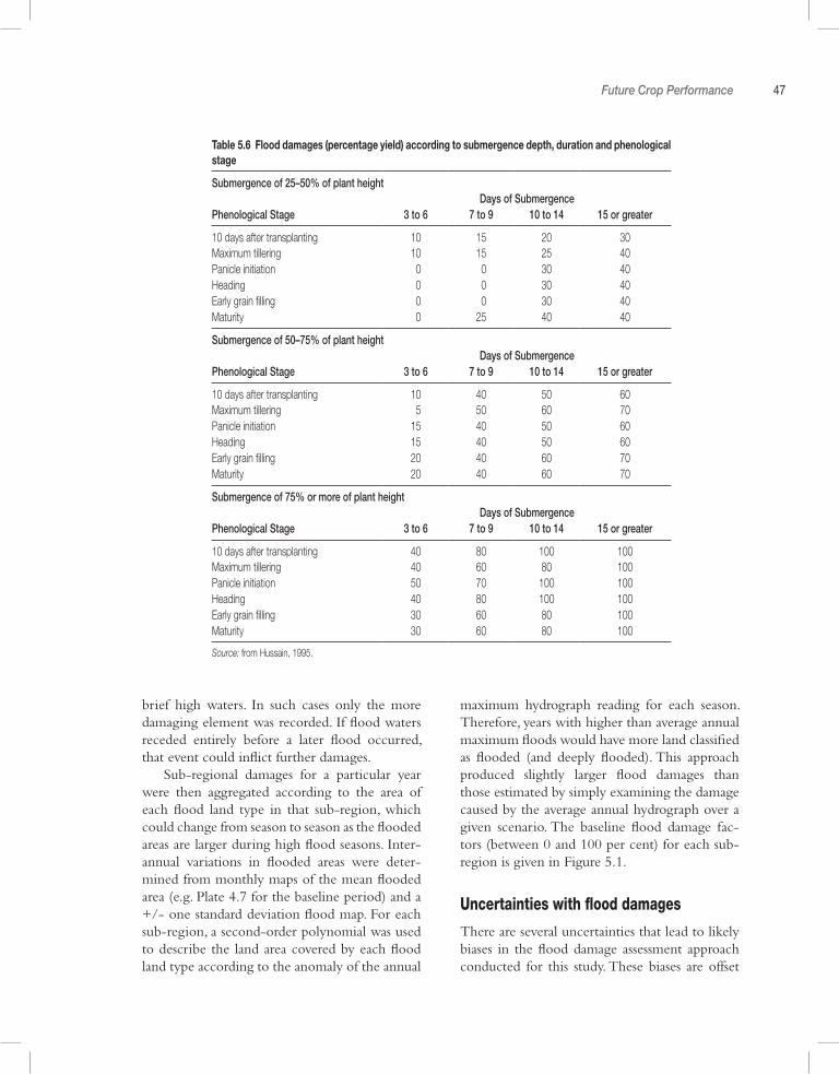
Future Crop Performance 47
brief high waters. In such cases only the more damaging element was recorded. If flood waters receded entirely before a later flood occurred, that event could inflict further damages.
Sub-regional damages for a particular year were then aggregated according to the area of each flood land type in that sub-region, which could change from season to season as the flooded areas are larger during high flood seasons. Inter-annual variations in flooded areas were deter-mined from monthly maps of the mean flooded area (e.g. Plate 4.7 for the baseline period) and a +/- one standard deviation flood map. For each sub-region, a second-order polynomial was used to describe the land area covered by each flood land type according to the anomaly of the annual
maximum hydrograph reading for each season. Therefore, years with higher than average annual maximum floods would have more land classified as flooded (and deeply flooded). This approach produced slightly larger flood damages than those estimated by simply examining the damage caused by the average annual hydrograph over a given scenario. The baseline flood damage fac-tors (between 0 and 100 per cent) for each sub-region is given in Figure 5.1.
Uncertainties with flood damages
There are several uncertainties that lead to likely biases in the flood damage assessment approach conducted for this study. These biases are offset
Table 5.6 Flood damages (percentage yield) according to submergence depth, duration and phenological stage
Submergence of 25–50% of plant heightDays of Submergence
Phenological Stage 3 to 6 7 to 9 10 to 14 15 or greater
10 days after transplanting 10 15 20 30Maximum tillering 10 15 25 40Panicle initiation 0 0 30 40Heading 0 0 30 40Early grain filling 0 0 30 40Maturity 0 25 40 40
Submergence of 50–75% of plant heightDays of Submergence
Phenological Stage 3 to 6 7 to 9 10 to 14 15 or greater
10 days after transplanting 10 40 50 60Maximum tillering 5 50 60 70Panicle initiation 15 40 50 60Heading 15 40 50 60Early grain filling 20 40 60 70Maturity 20 40 60 70
Submergence of 75% or more of plant heightDays of Submergence
Phenological Stage 3 to 6 7 to 9 10 to 14 15 or greater
10 days after transplanting 40 80 100 100Maximum tillering 40 60 80 100Panicle initiation 50 70 100 100Heading 40 80 100 100Early grain filling 30 60 80 100Maturity 30 60 80 100
Source: from Hussain, 1995.
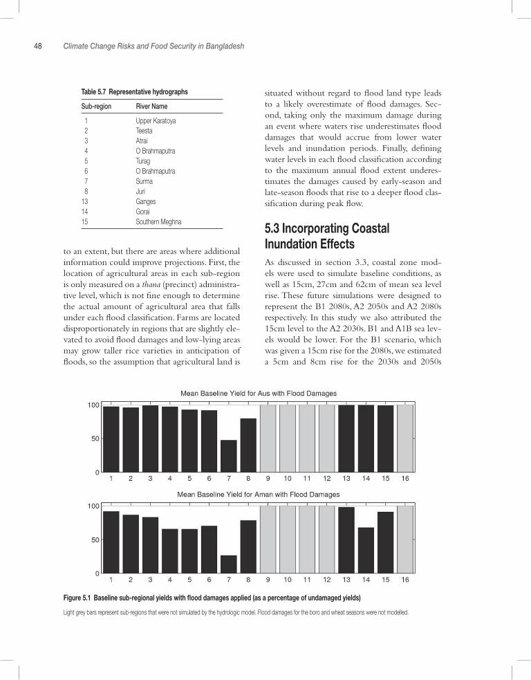
48 Climate Change Risks and Food Security in Bangladesh
to an extent, but there are areas where additional information could improve projections. First, the location of agricultural areas in each sub-region is only measured on a thana (precinct) administra-tive level, which is not fine enough to determine the actual amount of agricultural area that falls under each flood classification. Farms are located disproportionately in regions that are slightly ele-vated to avoid flood damages and low-lying areas may grow taller rice varieties in anticipation of floods, so the assumption that agricultural land is
situated without regard to flood land type leads to a likely overestimate of flood damages. Sec-ond, taking only the maximum damage during an event where waters rise underestimates flood damages that would accrue from lower water levels and inundation periods. Finally, defining water levels in each flood classification according to the maximum annual flood extent underes-timates the damages caused by early-season and late-season floods that rise to a deeper flood clas-sification during peak flow.
5.3 Incorporating Coastal Inundation EffectsAs discussed in section 3.3, coastal zone mod-els were used to simulate baseline conditions, as well as 15cm, 27cm and 62cm of mean sea level rise. These future simulations were designed to represent the B1 2080s, A2 2050s and A2 2080s respectively. In this study we also attributed the 15cm level to the A2 2030s. B1 and A1B sea lev-els would be lower. For the B1 scenario, which was given a 15cm rise for the 2080s, we estimated a 5cm and 8cm rise for the 2030s and 2050s
Table 5.7 Representative hydrographs
Sub-region River Name
1 Upper Karatoya 2 Teesta 3 Atrai 4 O Brahmaputra 5 Turag 6 O Brahmaputra 7 Surma 8 Juri13 Ganges14 Gorai15 Southern Meghna
Figure 5.1 Baseline sub-regional yields with flood damages applied (as a percentage of undamaged yields)
Light grey bars represent sub-regions that were not simulated by the hydrologic model. Flood damages for the boro and wheat seasons were not modelled.
Future Crop Performance 49
respectively. Since these lower values were not explicitly modelled, we estimated that their inun-dations were approximately linear proportions of the 15cm inundation maps. Since the publication of the IPCC Fourth Assessment Report (AR4), new research into ice dynamics in a warming climate suggest that sea level rise may occur more rapidly than previously thought (Alley et al, 2005; Copenhagen Diagnosis, 2009). As noted in Chapter 3, improved methods are available for re-estimating sea level rise.
Even with current sea levels, many coastal areas are periodically flooded with seawater due to tidal oscillations and river floods (see Plate 3.1). Areas that are classified as experiencing coastal floods of 30cm or more during the baseline period are assumed to have already abandoned grain production. Thus, impacts of sea level rise on agriculture can be assessed by removing sub-regional production according to the proportion of additional land lost under the future flooding scenarios.
Future agricultural impacts of sea level rise are likely biased by somewhat offsetting factors that were not modelled. Only mean sea level rise and tidal fluctuations were considered for this study, representing an optimistic scenario of coastal inundation. Additional land lost to extreme tidal and storm surges that can penetrate further up the distributaries along the Bang-ladesh coast were not considered, nor were the effects of salinity increases on soil, ground and irrigation water. However, agricultural land in these areas was assumed to be distributed without regard for potential coastal inundation, leading to a likely overestimate of sea level rise damage. Also not considered was the salinity impact of farm-ers who convert their fields to aquaculture (e.g. shrimp) by inundating their land with saltwater.
5.4 Projections of Future Potential Unflooded Production (Climate Only)As discussed in section 4.3, a ‘delta’ approach is used for generating future climate scenarios whereby climate changes from a particular model experiment are applied directly to the BMD
observational data. This adjusted observational climate data is used directly in DSSAT. Thus, these scenarios are plausible climate conditions that retain the day-to-day and year-to-year char-acteristics of the 1970–99 baseline period, with monthly mean temperatures and precipitation that reflect the mean climate changes simulated by the GCM/emissions scenarios for the 2030s, 2050s and 2080s. By adjusting according to monthly means, changes in seasonality simulated by a given model experiment are also captured. The entire set of GCMs (Table 3.1), all three emissions scenarios and all future time slices are utilized.
In the initial simulations of future changes in potential unflooded yield (before the applica-tion of flood and sea level damages), crops are affected by CO
2 concentration, temperature and
precipitation changes. These factors interact in a non-linear manner, but an estimate of the relative contribution of the CO
2 concentration com-
pared to the effects of changing temperature and precipitation may be attained through test simu-lations. Both rice and wheat are C3 crops, and thus both react strongly to changes in tempera-ture and CO
2 concentrations (Kimball and Ber-
nacchi, 2006; Hatfield et al, 2008). The isolated impacts of changing CO
2 concentrations, as well
as of changing precipitation and temperature, are described in this section, along with their com-bined direct effect of changing climate in each sub-region. Figure 5.2 summarizes the results as changes in national potential production due to isolated and combined direct climate effects.
CO2 impact experiments
To isolate the agricultural effects of increased CO
2 concentration predicted by climate change,
future climate scenarios were generated that used the baseline temperature and precipitation data but used CO
2 levels to match the future scenarios
(see Table 5.8). Thus, the only difference between the future experiments and the baseline condi-tions was an elevated CO
2 concentration. Because
the same CO2 levels were used for all GCMs in
a particular emissions scenario, a single 30-year simulation for each crop in each sub-region
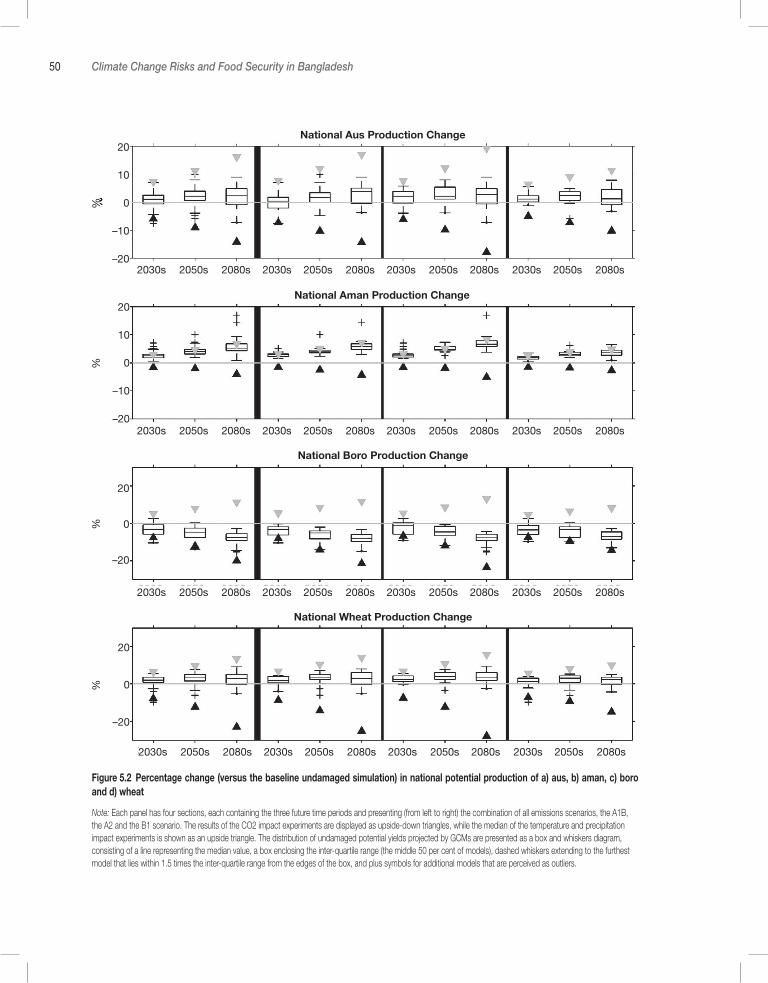
50 Climate Change Risks and Food Security in Bangladesh
Figure 5.2 Percentage change (versus the baseline undamaged simulation) in national potential production of a) aus, b) aman, c) boro and d) wheat
Note: Each panel has four sections, each containing the three future time periods and presenting (from left to right) the combination of all emissions scenarios, the A1B, the A2 and the B1 scenario. The results of the CO2 impact experiments are displayed as upside-down triangles, while the median of the temperature and precipitation impact experiments is shown as an upside triangle. The distribution of undamaged potential yields projected by GCMs are presented as a box and whiskers diagram, consisting of a line representing the median value, a box enclosing the inter-quartile range (the middle 50 per cent of models), dashed whiskers extending to the furthest model that lies within 1.5 times the inter-quartile range from the edges of the box, and plus symbols for additional models that are perceived as outliers.
National Aus Production Change
National Aman Production Change
National Boro Production Change
National Wheat Production Change
20
10
0
–10
–20
20
10
0
–10
–20
20
0
–20
20
0
–20
2030s 2050s 2080s 2030s 2050s 2080s 2030s 2050s 2080s 2030s 2050s 2080s
2030s 2050s 2080s 2030s 2050s 2080s 2030s 2050s 2080s 2030s 2050s 2080s
2030s 2050s 2080s 2030s 2050s 2080s 2030s 2050s 2080s 2030s 2050s 2080s
2030s 2050s 2080s 2030s 2050s 2080s 2030s 2050s 2080s 2030s 2050s 2080s
%%
%%
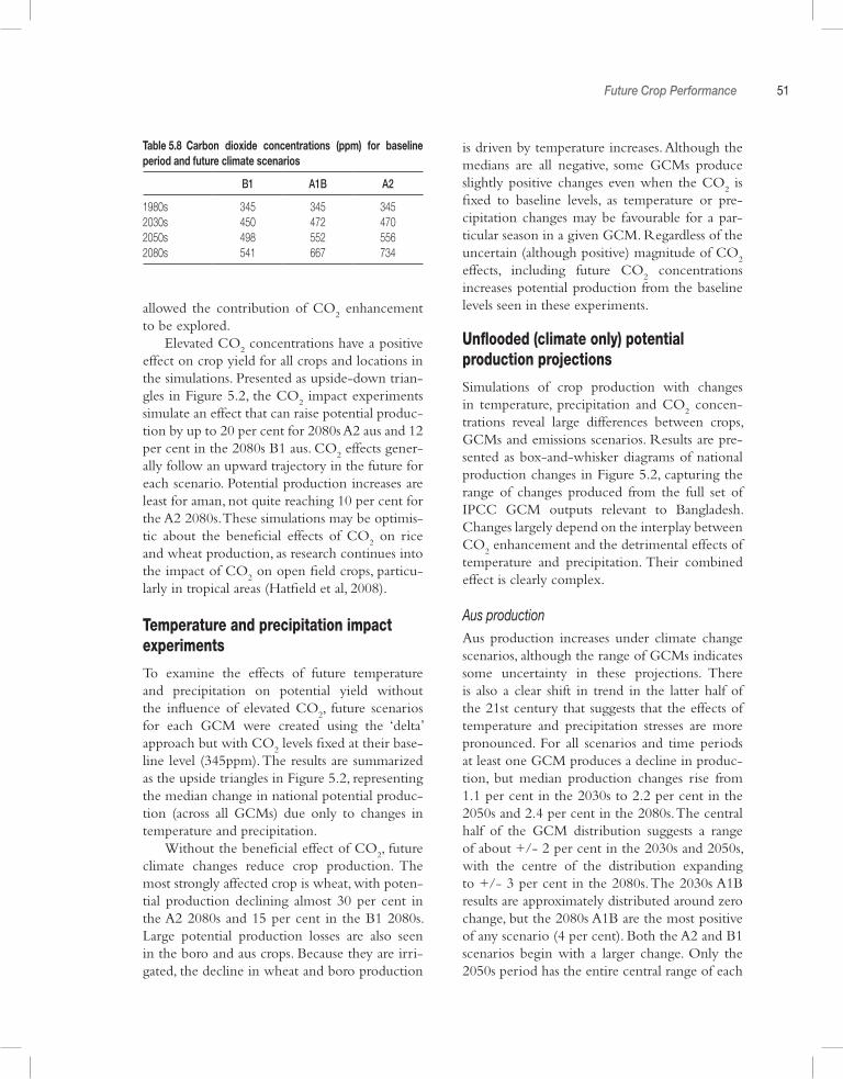
Future Crop Performance 51
allowed the contribution of CO2 enhancement
to be explored. Elevated CO
2 concentrations have a positive
effect on crop yield for all crops and locations in the simulations. Presented as upside-down trian-gles in Figure 5.2, the CO
2 impact experiments
simulate an effect that can raise potential produc-tion by up to 20 per cent for 2080s A2 aus and 12 per cent in the 2080s B1 aus. CO
2 effects gener-
ally follow an upward trajectory in the future for each scenario. Potential production increases are least for aman, not quite reaching 10 per cent for the A2 2080s. These simulations may be optimis-tic about the beneficial effects of CO
2 on rice
and wheat production, as research continues into the impact of CO
2 on open field crops, particu-
larly in tropical areas (Hatfield et al, 2008).
Temperature and precipitation impact experiments
To examine the effects of future temperature and precipitation on potential yield without the influence of elevated CO
2, future scenarios
for each GCM were created using the ‘delta’ approach but with CO
2 levels fixed at their base-
line level (345ppm). The results are summarized as the upside triangles in Figure 5.2, representing the median change in national potential produc-tion (across all GCMs) due only to changes in temperature and precipitation.
Without the beneficial effect of CO2, future
climate changes reduce crop production. The most strongly affected crop is wheat, with poten-tial production declining almost 30 per cent in the A2 2080s and 15 per cent in the B1 2080s. Large potential production losses are also seen in the boro and aus crops. Because they are irri-gated, the decline in wheat and boro production
is driven by temperature increases. Although the medians are all negative, some GCMs produce slightly positive changes even when the CO
2 is
fixed to baseline levels, as temperature or pre-cipitation changes may be favourable for a par-ticular season in a given GCM. Regardless of the uncertain (although positive) magnitude of CO
2
effects, including future CO2 concentrations
increases potential production from the baseline levels seen in these experiments.
Unflooded (climate only) potential production projections
Simulations of crop production with changes in temperature, precipitation and CO
2 concen-
trations reveal large differences between crops, GCMs and emissions scenarios. Results are pre-sented as box-and-whisker diagrams of national production changes in Figure 5.2, capturing the range of changes produced from the full set of IPCC GCM outputs relevant to Bangladesh. Changes largely depend on the interplay between CO
2 enhancement and the detrimental effects of
temperature and precipitation. Their combined effect is clearly complex.
Aus productionAus production increases under climate change scenarios, although the range of GCMs indicates some uncertainty in these projections. There is also a clear shift in trend in the latter half of the 21st century that suggests that the effects of temperature and precipitation stresses are more pronounced. For all scenarios and time periods at least one GCM produces a decline in produc-tion, but median production changes rise from 1.1 per cent in the 2030s to 2.2 per cent in the 2050s and 2.4 per cent in the 2080s. The central half of the GCM distribution suggests a range of about +/- 2 per cent in the 2030s and 2050s, with the centre of the distribution expanding to +/- 3 per cent in the 2080s. The 2030s A1B results are approximately distributed around zero change, but the 2080s A1B are the most positive of any scenario (4 per cent). Both the A2 and B1 scenarios begin with a larger change. Only the 2050s period has the entire central range of each
Table 5.8 Carbon dioxide concentrations (ppm) for baseline period and future climate scenarios
B1 A1B A2
1980s 345 345 3452030s 450 472 4702050s 498 552 5562080s 541 667 734
52 Climate Change Risks and Food Security in Bangladesh
scenario simulation higher than zero change. Aus production changes are fairly evenly distributed between the CO
2 impact and the temperature
and precipitation impact experiment results.
Aman productionAman production rises under all future time periods, emissions scenarios and GCM simu-lations. Following rising CO
2 concentrations,
median production changes increase with time to 2 per cent in the 2030s to 4 per cent in the 2050s and to 5 per cent in the 2080s. Aman rice has the most robust changes of any crop, show-ing remarkably low variability between different scenarios. Overall changes are relatively small, however, with only a few GCM scenarios caus-ing rises of 10 per cent or more. The centre half of the simulation distributions range around +/- 0.5 per cent in the 2030s, rising to +/- 1 per cent by the 2080s when emissions scenarios are combined. This increase in range is due mostly to the diverging emissions scenarios, which drive significantly different CO
2 enhancement impacts.
Aman rice is grown at the height of the mon-soon season, which provides plenty of rain even in simulations where mean rainfall decreases slightly. Monsoon clouds and high humidity also keep temperatures lower than in the pre-mon-soon period. These factors reduce the tempera-ture and precipitation impacts of climate change, and cause the production to be influenced most strongly by the beneficial CO
2 enhancement.
Some scenarios even produce better production gains than the CO
2 enrichment alone, suggesting
that the temperature and precipitation character-istics are more favourable for aman production. These results are in the absence of flood impacts discussed in subsequent sections.
Boro productionBoro production declines under climate change scenarios, with median national production losses across all emissions scenarios reaching 3 per cent in the 2030s, 5 per cent in the 2050s and 8 per cent in the 2080s. Several simulations project decreases in production of more than 10 per cent, with one GCM projecting a 15 per cent decline
in the 2080s A1B. The central portion of the boro distributions ranges around +/- 2 per cent, and the distributions grow tighter at the end of the 21st century. Boro production changes are more responsive to the temperature changes than the CO
2 enhancement, with irrigation offsetting any
precipitation change. Note that these estimates are conservative given that groundwater irriga-tion is assumed to be unconstrained. Currently, with evidence of declining groundwater tables in many parts of the northwest, future water avail-ability may pose a serious additional constraint on boro production.
Wheat productionWheat production increases under most climate change scenarios, although there is a clear shift in trend at the end of the 21st century towards lower yields. Median increases across all scenar-ios are 2 per cent, 4 per cent and 3 per cent for 2030s 2050s, and 2080s respectively. The largest median increases in yield for all emission scenar-ios occur in the 2050s, with A2 production rising 4 per cent, B1 production rising 3 per cent and the centre of the distribution ranging +/- 2 per cent. Potential production tracks more closely with the CO
2 enhancement than with the detri-
mental temperature increases (irrigation negates precipitation changes), but toward the end of the century production begins to move away from the CO
2 influence toward the much lower tem-
perature impacts.
5.5 Projections of Future Projected Flood DamagesProduction changes due to flood damages are presented in Figure 5.3 for aus and aman rice (boro and wheat are assumed to be un-impacted by floods). Flood damages are projected to increase in most scenarios, particularly for the 2050s time period and for the aman crop grown at the height of the monsoon. Median additional losses across all scenarios are 1 per cent and 2 per cent in the 2030s and 2050s respectively. Maxi-mum median flood losses occur in the 2050s A2, with national aman production falling 4 per cent

Future Crop Performance 53
and national aus production dropping 2.4 per cent. More modest crop losses are projected for the B1 scenario, reaching only 1 per cent of aus production and 3 per cent of aman production in the 2050s. The narrow distribution of flood damages projected by different GCMs suggests a robust change, although changes are small com-pared to the year-to-year variability in each time period. These results are likely to be optimistic, as changes in inter-annual variability between the baseline and future time periods are likely to produce larger flood damages and several sub-regions were not modelled.
5.6 Projections of Potential Coastal Inundation DamagesThe percentage of production lost to coastal inundation associated with sea level rise in each sub-region is presented in Figure 5.4. Coastal
sub-regions experience impacts that increase with time as sea levels rise, with maximum crop losses of nearly 40 per cent projected for the 2080s in sub-region 16 in the southwest. Sub-region 15 also loses a substantial portion of agri-cultural production, while more modest losses are simulated in sub-regions 10 and 12. Even without considering the effects of increased fre-quency of cyclones and increasing groundwater salinity, these simulations still project consider-able production losses.
5.7 Projections of Integrated Damages
National production changes
The combined impacts of climate change on potential national cereal production are pre-sented in Figure 5.5, including the effects of CO
2
Figure 5.3 Percentage change (versus the baseline flood-only simulation) in national potential production affected by basin floods of a) aus and b) aman (boro and wheat are assumed to be flood-free)
Note: Each panel has three sections, each containing the two future time periods and presenting (from left to right) the combination of all emissions scenarios, the A2 scenario and the B1 scenario. The distribution of flood-damaged potential yields projected by GCMs is presented as a box and whiskers diagram, consisting of a line representing the median value, a box enclosing the inter-quartile range (the middle 50 per cent of models), dashed whiskers extending to the furthest model that lies within 1.5 times the inter-quartile range from the edges of the box, and plus symbols for additional models that are perceived as outliers.
National Aus Production Changes – Food Damages Only
National Aman Production Changes – Food Damages Only
10
5
0
–5
–10
%%
10
5
0
–5
–10
ALL 2030s ALL 2050s A2 2030s A2 2050s B1 2030s B1 2050s
ALL 2030s ALL 2050s A2 2030s A2 2050s B1 2030s B1 2050s
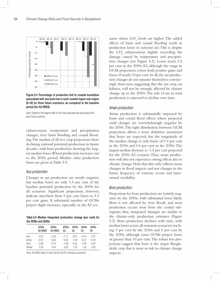
54 Climate Change Risks and Food Security in Bangladesh
enhancement, temperature and precipitation changes, river basin flooding and coastal flood-ing. The median of all rice crop projections show declining national potential production in future decades, with boro production showing the larg-est median losses. Wheat production increases out to the 2050s period. Median value production losses are given in Table 5.9.
Aus productionChanges in aus production are mostly negative, but median losses are only 1.5 per cent of the baseline potential production by the 2050s for all scenarios. Significant projections, however, indicate anywhere from 9 per cent losses to 3.5 per cent gains. A substantial number of GCMs project slight increases, especially in the A2 sce-
nario where CO2 levels are higher. The added
effects of basin and coastal flooding result in production losses in national aus. This is despite the CO
2 enhancement slightly exceeding the
damage caused by temperature and precipita-tion changes (see Figure 5.2). Losses reach 3.5 per cent in the 2050s A2, although the range in GCM projections covers both positive gains and losses of nearly 10 per cent. In all, the aus produc-tion changes do not separate themselves convinc-ingly from zero, suggesting that the aus crop, on balance, will not be strongly affected by climate change up to the 2050s. The role of aus in total production is expected to decline over time.
Aman productionAman production is substantially impacted by basin and coastal flood effects where projected yield changes are overwhelmingly negative by the 2050s. The tight distribution between GCM projections allows a more definitive assessment that losses are expected, but the magnitude of the median change is only losses of 0.4 per cent in the 2030s and 0.6 per cent in the 2050s. The largest median decrease is -1.5 per cent projected for the 2050s A2 scenario. Thus, aman produc-tion will also not experience strong effects due to climate change. Note that this only reflects mean changes in flood impacts and not changes in the future frequency of extreme events and inter-annual variability.
Boro productionProjections for boro production are entirely neg-ative by the 2050s, with substantial losses likely. Boro is not affected by river floods, and most production occurs away from the coastal sub-regions; thus, integrated damages are similar to the climate-only production estimates (Figure 5.2). Boro production declines with time, with median losses across all emissions scenarios reach-ing 3 per cent by the 2030s and 5 per cent by the 2050s, although some GCMs project losses of greater than 10 per cent. The robust loss pro-jections suggest that boro is the major Bangla-deshi crop that is most at-risk to climate change impacts.
Figure 5.4 Percentage of production lost to coastal inundation associated with sea level rise in each coastal region sub-region (9–16) for three future scenarios, as compared to the baseline period (for A2 SRES)
Note: Depths in the legend refer to the mean sea level rise associated with each future scenario.
Table 5.9 Median integrated production change (per cent) for the 2030s and 2050s
2030s 2050s 2030s 2050s 2030s 2050sAll SRES All SRES A2 A2 B1 B1
Aus –0.27 –1.52 –1.11 –3.51 –0.14 –0.01Aman –0.37 –0.62 –0.42 –1.49 –0.37 –0.40Boro –3.06 –4.74 –1.68 –5.54 –3.76 –3.54Wheat –2.05 –3.44 –2.23 –3.74 –1.33 –3.03
Note: All SRES refers to both the A2 and B1 emissions scenarios
SR-09 SR-10 SR-11 SR-12 SR-13 SR-14 SR-15 SR-160
–5
–10
–15
–20
–25
–30
–35
–40
Per
cent
age
pro
duc
tion
chan
ge
2030s (15 cm)
2050s (27 cm)
2080s (62 cm)

Future Crop Performance 55
Figure 5.5 Percentage change (versus the baseline flood-affected simulation) in national potential production with the combined effects of CO2, temperature and precipitation changes, basin flooding and coastal flooding
Note: Each panel has three sections, each containing two future time periods and presenting (from left to right) the combination of all emissions scenarios, the A2 scenario and the B1 scenario. The distribution of potential yields projected by GCMs are presented as a box and whiskers diagram, consisting of a line representing the median value, a box enclosing the inter-quartile range (the middle 50 per cent of models), dashed whiskers extending to the furthest model that lies within 1.5 times the inter-quartile range from the edges of the box, and plus symbols for additional models that are perceived as outliers.
National Aus Production Changes – All Impacts
10
0
–10
%
ALL 2030s ALL 2050s A2 2030s A2 2050s B1 2030s B1 2050s
National Aman Production Changes – All Impacts
National Boro Production Changes – All Impacts
National Wheat Production Changes – All Impacts
ALL 2030s ALL 2050s A2 2030s A2 2050s B1 2030s B1 2050s
ALL 2030s ALL 2050s A2 2030s A2 2050s B1 2030s B1 2050s
ALL 2030s ALL 2050s A2 2030s A2 2050s B1 2030s B1 2050s
10
0
–10
%
10
0
–10
%
10
0
–10
%
56 Climate Change Risks and Food Security in Bangladesh
Wheat productionWheat production increases under climate change, reaching nearly 4 per cent in the 2050s A2. Some GCMs project gains as high as 7 per cent in that period, but some B1 scenarios project production losses when CO
2 levels are
not as high. Wheat does not experience river flooding and most production occurs away from coastal regions affected by sea level rise, so inte-grated estimates are very similar to the undam-aged production estimates above (Figure 5.2). In all, wheat production is projected to be positively affected by climate change out to the 2050s, but strong temperature effects (represented as upside triangles in Figure 5.2d) and uncertain benefits of enhanced CO
2 concentrations suggest that these
wheat gains may be overly optimistic. These sim-ulations also indicate that wheat production may decline rapidly as temperature changes pass key thresholds.
Sub-regional production changes
Figure 5.6 and Table 5.10 show the production changes by crop, by climate impact factor and by sub-region for the 2050s for a combined A2 and B1 scenarios. Production losses compared to the baseline are estimated for at least one crop in each sub-region. For sub-regions including Maijdee Court (SR-12), Patuakhali (SR-15) and Khulna (SR-16), the yields for all four crops are reduced. These southern areas are the most vul-nerable to climate change due primarily to both sea level rise and riverine flooding. The larg-est observed decreases in yields are in Khulna (SR-16) (approximately 10 per cent reduction in aman, aus and wheat yields, and 18 per cent reduction in boro yields). For five sub-regions – Tangail (SR-4), Sylhet (SR-7), Maijdee Court (SR-12), Patuakhali (SR-15) and Khulna (SR-16) – both the aman and aus crops demonstrate negative changes in yields. That is, any poten-tial gains from CO
2 effects on the aus and aman
will be more than offset by the negative impacts of temperature and precipitation changes, and inland and coastal flooding. For the wheat crop, only five sub-regions show decreases in yields. These are concentrated in the south where wheat
production is lower. For the boro crop, all but one sub-region, Sylhet (SR-7), show decreases in yields (primarily due to CO
2 fertilization effects).
The largest decrease in yield from basin flood-ing is observed in sub-region 7 (approximately 9 per cent for both the aman and aus crop). For coastal flooding, the largest decreases in yield are observed in SR-12, SR-15 and SR-16 (7 per cent, 9 per cent and 13 per cent reductions respectively). The yield impacts of temperature and precipitation changes vary by sub-region depending on the crop. The largest declines in aman, aus, boro and wheat are in SR-3 (4 per cent), SR-4 (13 per cent), SR-8 (16 per cent) and SR-1 (19 per cent) respectively.
5.8 Using the Crop Model to Simulate Adaptation OptionsVulnerabilities to and potential adaptation strat-egies for climate change have been identified in Bangladesh for agriculture and many other sectors (Karim et al, 1994; Huq et al, 1999; Ali, 1999; NAPA, 2005; Ahmed, 2006; Tanner et al, 2007). The IPCC also devoted chapters to glo-bal climate change impacts on the agricultural sector (Easterling et al, 2007) and coastal regions (Nicholls et al, 2007) as well as adaptation options (Adger et al, 2007). Thomalla et al (2005) detail some of the historical efforts to implement wide-spread adaptation strategies in Bangladesh utiliz-ing local, regional, governmental and non-gov-ernmental entities. Much of the international effort for adaptation has focused on reducing the threats of floods and tropical cyclones follow-ing devastating events in the 1980s and 1990s. Some agricultural adaptation is already being tested in the field, e.g. dried hyacinth used as a basis for floating agriculture during flooding in Barisal and salinity-tolerant cultivars introduced to adapt to salinity intrusion (Sarwar, 2005). But widespread efforts in the agricultural sector are not yet prominent. Moreover, the current large gap between actual and potential yields suggests substantial on-farm opportunities for growth and poverty reduction. Expanded availability of mod-ern rice varieties, irrigation facilities, fertilizer use
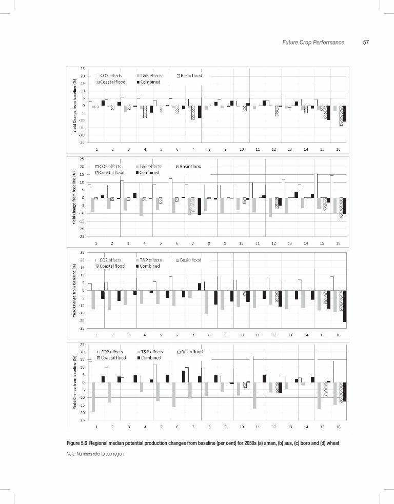
Future Crop Performance 57
Figure 5.6 Regional median potential production changes from baseline (per cent) for 2050s (a) aman, (b) aus, (c) boro and (d) wheat
Note: Numbers refer to sub-region.
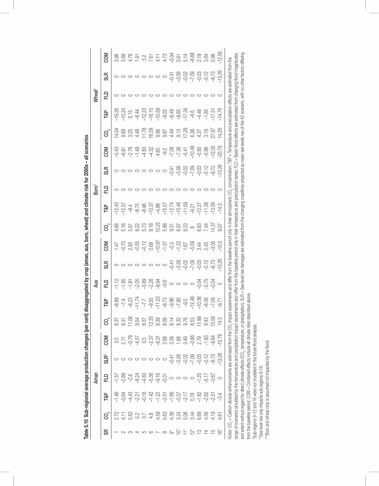
Tabl
e 5.
10 S
ub-re
gion
al a
vera
ge p
rodu
ctio
n ch
ange
s (p
er c
ent)
disa
ggre
gate
d by
cro
p (a
man
, aus
, bor
o, w
heat
) and
clim
ate
risk
for 2
050s
– al
l sce
nario
s
Aman
Aus
Boro
1W
heat
1
SRCO
2T&
PFL
DSL
R2CO
MCO
2T&
PFL
DSL
RCO
MCO
2T&
PFL
DSL
RCO
MCO
2T&
PFL
DSL
RCO
M
12.
72–1
.46
–1.5
70
3.5
8.37
–8.8
9–1
.12
01.
474.
66–1
2.43
00
–5.4
314
.04
–19.
260
03.
962
4.11
–0.6
4–2
.69
02.
718.
31–7
.4–1
.95
0–0
.75
5.16
–12.
570
0–6
.81
9.69
–13.
240
03.
883
5.83
–4.4
3–2
.80
–0.7
811
.06
–8.2
3–1
.91
02.
935.
91–9
.40
0–2
.78
3.25
0.15
00
4.76
45.
2–2
.21
–8.2
40
–4.5
79.
54–1
1.74
–2.0
50
–0.5
58.
22–8
.75
00
–1.4
94.
48–6
.44
00
1.91
53.
7–0
.16
–4.8
30
0.5
8.37
–7.7
–3.8
90
–0.1
25.
73–8
.96
00
–4.8
311
.78
–12.
230
05.
26
4.8
–1.4
2–5
.38
0–2
.37
12.3
5–9
.55
–2.2
80
0.68
9.18
–10.
370
0–4
.32
16.5
9–1
6.15
00
7.61
74.
59–1
.22
–9.1
60
–8.3
18.
39–1
1.23
–8.9
40
–10.
9710
.25
–4.8
80
04.
839.
98–1
0.59
00
4.11
85.
63–2
.51
–0.3
10
2.68
8.56
–8.7
3–0
.60
–1.0
75.
88–1
5.57
00
–9.2
9.87
–9.0
20
04.
739*
4.38
–1.6
60
–0.4
13.
398.
14–9
.96
0–0
.41
–0.3
9.31
–12.
740
–0.4
1–7
.08
4.49
–6.4
90
–0.4
1–0
.94
10*
3.24
–0.5
70
–3.5
61.
688.
32–7
.92
0–3
.56
–1.2
26.
97–1
0.46
0–3
.56
–7.3
89.
13–8
.65
0–3
.56
0.61
11*
5.06
–2.1
70
–0.0
23.
499.
76–9
.50
–0.0
21.
678.
23–1
1.59
0–0
.02
–5.4
117
.28
–17.
340
–0.0
25.
1412
*3.
440.
780
–7.0
9–0
.66
8.53
–12.
480
–7.0
9–5
.09
8–9
.21
0–7
.09
–10.
496.
38–6
.60
–7.0
9–6
.68
136.
69–1
.82
–1.2
5–0
.03
2.79
11.9
9–1
0.36
–0.0
4–0
.03
3.44
6.63
–12.
270
–0.0
3–5
.85
4.37
–4.4
60
–0.0
32.
1914
4.56
–2.6
2–5
.17
–0.1
2–1
.83
8.43
–6.5
8–0
.75
–0.1
22.
437.
44–1
1.39
0–0
.12
–5.9
83.
19–1
.85
0–0
.12
3.64
154.
19–2
.51
–3.6
7–8
.73
–9.6
415
.58
–7.0
9–0
.04
–8.7
3–3
.05
14.3
7–1
3.09
0–8
.73
–12.
0527
.97
–17.
510
–8.7
30.
9616
*4.
61–3
.40
–13.
26–1
0.76
14.3
–9.7
10
–13.
26–1
0.5
9.07
–14.
30
–13.
26–2
0.79
14.2
6–1
4.76
0–1
3.26
–12.
56
Note
s: CO
2 = C
arbo
n dio
xide
enha
ncem
ents
are
estim
ated
from
the
CO2 im
pact
exp
erim
ents
and
differ
from
the
base
line
perio
d on
ly in
their
atm
osph
eric
CO2 c
once
ntra
tion;
T&P
= Te
mpe
ratu
re a
nd p
recip
itatio
n eff
ects
are
estim
ated
from
the
rang
e of
scen
arios
sim
ulate
d by
the
tem
pera
ture
and
pre
cipita
tion
impa
ct e
xper
imen
ts an
d dif
fer fr
om th
e ba
selin
e pe
riod
only
in th
eir te
mpe
ratu
re a
nd p
recip
itatio
n se
ries;
FLD
= Ba
sin flo
od e
ffect
s are
esti
mat
ed fr
om c
hang
ing flo
od m
agnit
udes
an
d ex
tent
with
out r
egar
d fo
r dire
ct c
limat
e eff
ects
(CO 2, t
empe
ratu
re, o
r pre
cipita
tion);
SLR
= S
ea le
vel ri
se d
amag
es a
re e
stim
ated
from
the
chan
ging
coas
tlines
pro
jecte
d as
mea
n se
a lev
els ris
e of
the
A2 sc
enar
io, w
ith n
o ot
her f
acto
rs d
ifferin
g fro
m th
e ba
selin
e pe
riod;
COM
= C
ombin
ed e
ffect
s inc
lude
all c
limat
e ris
ks d
escr
ibed
abov
e.*S
ub-re
gions
9–1
2 an
d 16
wer
e no
t mod
elled
in th
e fu
ture
flood
ana
lysis.
**Sea
leve
l rise
only
impa
cts s
ub-re
gions
9–1
6.***
Boro
and
whe
at c
rop
is as
sum
ed n
ot im
pact
ed b
y the
flood
.
Future Crop Performance 59
and labour could increase average yields at rates that dwarf the climate change impacts.
An important follow-on to the present study is the use of the crop simulation approach devel-oped here to evaluate adaptive responses them-selves. There are many elements of cropping for which adaptations can be studied; these are described in detail in Annex 1. The elements for potential evaluation include: cultivar selec-
tion; adjustments in planting and harvesting dates and crop sequence; changes in planting systems, including crop density; and input adjustments including irrigation, fertilizer and farm-level environmental modifications. Studying these elements will enable the development of addi-tional adaptation options such as those detailed in Chapter 7.
6
Economy-wide Impacts of Climate Risks
Box 6.1 Key messages
• Economy-wide adjustments will to some extent mitigate the physical losses predicted.• Existing climate variability has a pronounced detrimental economy-wide impact. Compared to an
‘optimal’ climate simulation with the highest simulated yield and no inter-annual variations, climate variability is estimated to reduce long-term rice production by an average 7.4 per cent each year during 2005–50, primarily by lowering production of the aman and aus crops. Average annual rice production growth is lowered in all sub-regions.
• Simulated climate variability is projected to cost the agriculture sector (in discounted terms) US$26 billion in agricultural GDP during the 2005–50 simulation period (US$0.57 billion per year in 2005 US$) compared with optimal production and growth. This climate variability has economy-wide impli-cations beyond simply the size-effect of the lost agricultural GDP. Existing climate variability is esti-mated to cost Bangladesh US$121 billion in lost national GDP during the same period (US$3 billion per year).
• Climate change exacerbates the negative impacts of existing climate variability for food security by further reducing rice production by a projected cumulative total of 80Mt over the 2005–50 simulation period (3.9 per cent each year), driven primarily by reduced boro crop production. This is equivalent to almost two years’ worth of rice production lost over the next 45 years as a result of climate change. Uncertainty about future climate change means that annual rice production losses range between 3.6 per cent and 4.3 per cent.
• Climate change primarily impacts boro rice and thus limits its ability to compensate for lost aus and aman rice production during extreme events.
• Agricultural GDP is projected to be 3.1 per cent lower each year as a result of climate change (US$8 billion in lost value-added in 2005 US$). Average loss in agricultural GDP due to climate change is estimated to be a third of the agricultural GDP losses associated with existing climate variability. This is projected to cost Bangladesh US$26 billion in total GDP over the 2005–50 period. This is equiva-lent to US$570 million overall lost each year to climate change, or alternatively an average annual 1.15 per cent reduction in total GDP by 2050.
• Uncertainty surrounding GCMs and emission scenarios means that costs may be as high as US$1 billion per year over 2005–50 under less optimistic scenarios.
• These climate risks will have severe implications for household welfare. For both the climate variability and climate change simulations, around 80 per cent of these losses fall directly on household con-sumption (cumulative total consumption losses of US$441.7 billion and US$104.7 billion for climate variability and climate change respectively).
• About 80 per cent of the projected economic losses from existing climate variability and climate change occur outside of the agriculture sector (from a national accounts perspective), particularly in the upstream and downstream agriculture value-added processing sectors. This means that both rural and urban households may be adversely affected.
Economy-wide Impacts of Climate Risks 61
Chapter 5 provides estimates of changes in pro-duction for four different crops (aus, aman, boro and wheat) due to various climate risks. Though informative, this information should be supple-mented by economic responses to these produc-tion shocks (e.g. land and labour reallocation, price effects). These economic adjustments will to some degree mitigate the physical losses pre-dicted. What is described in this section is the development and use of a dynamic computable general equilibrium model to assess the econ-omy-wide impacts from these projected losses. The focus here is on rice production economic impacts only since this dominates agricultural and household food consumption.
6.1 Integrating Climate Effects in an Economy-wide Model
Conceptual framework of the methodology
A dynamic computable general equilibrium (CGE) model was developed to estimate the impacts of existing climate variability and future climate change in Bangladesh on the agriculture sector. The yield change estimates from the hydro-crop models described earlier are passed down to the CGE model to estimate their economy-wide implications, including changes in production and household consumption for different sectors, household groups and sub-regions in the coun-try. A detailed description of the model is pro-vided in Annex 2.
Three impact channels, apart from crop yield changes estimated from the hydro-crop models, are captured in the CGE model. First, the CGE model includes the additional impacts that occur under extreme climatic events, such as during the major floods of 1988 and 1998. These comprise, for example, major losses of cultivatable land due to floodwater inundation, which occurs over and above the average flood yield losses described in previous sections. The second additional impact channel considered in the CGE analysis is the change in the frequency of these extreme events caused by climate change. It is expected that
major floods in Bangladesh will become more frequent, thus exacerbating economic losses through heightened climate variability. Finally, though sea level rise impacts on yields were determined earlier (see section 5.6) changes in cultivable land are explicitly incorporated in the CGE. The CGE analysis, therefore, builds on the hydro-crop modelling analysis by incorporat-ing the predicted crop yield changes, while also extending the analysis by including the impact and frequency of extreme climate events.
Climate simulations
Three sets of simulations are run using the CGE model.
Optimal ClimateThe first simulation is the ‘Optimal Climate Simulation’, in which Bangladesh is unaffected by existing climate variability or future climate change. This means that the highest simulated crops yields are used and sector productivity and factor supplies increase smoothly at long-term growth rates with no inter-annual variations. ‘Optimal’ is defined as the best simulated crop yield achieved in each sub-region during the 30-year baseline period 1970–99. This scenario reflects a hypothetical trajectory for Bangladesh in which there are no yield losses caused by cli-mate variability. This simulation provides a hypo-thetical baseline scenario against which other climate-affected simulations can be compared. Since climate conditions are always assumed to be ‘optimal’ (i.e. no crop yield losses or major floods), it is not necessary to run multiple base-line simulations to account for climate uncer-tainty (i.e. there is only one optimal scenario).
Existing VariabilityThe second set of simulations is the ‘Existing Variability Simulation’. These simulations include the yield losses associated with the historical cli-mate data series. The CGE model is run forward over 45 years (2005–50) and for each year a random observation is drawn from the histori-cal data series (1970–99). The crop yield changes
62 Climate Change Risks and Food Security in Bangladesh
estimated by the hydro-crop models (relative to the potential yields) for that particular base-line historical year are imposed on the CGE model, which then estimates the economy-wide impacts. Moreover, years in the historical record during which major floods took place (i.e. 1970, 1974, 1984, 1987, 1988 and 1998) are identified. If one of these years is drawn during the random selection, then additional impacts are imposed on the CGE model (discussed later in this sec-tion). Together these random selections from the historical climate data produce a single 45-year climate scenario based on existing climate variability and patterns (i.e. without the effects of climate change). This Monte Carlo process is repeated 50 times in order to produce a series of 45-year climate scenarios. The average economy-wide outcomes for these 50 simulations provide an estimate of the economic impact of existing climate variability since all Monte Carlo runs are considered equally likely.
Climate ChangeThe third set of simulations is the ‘Climate Change Simulation’. As described earlier, the hydro-crop models estimate crop yield changes for future 30-year time slices around the 2030s and 2050s based on a range of model experi-ments. As the CGE model is run forward over the 2005–50 period, yield impacts are drawn ini-tially from the historical series and then gradually from the future series. For example, there are 30 years separating the 2005 base year of the CGE model and the mid-point of the 2030s time slice. Thus, in 2010, which is year 5, 25/30 of the yield impact from the randomly selected year in the historical dataset and 5/30 of the yield impact from the same year in the 2030s time slice are used1. A similar linear transition from the 2030s to the 2050s time-series is used. As with the Existing Variability Simulation, this Monte Carlo process is repeated 50 times and the average is taken to provide an overall estimate of economic outcomes under climate change. Finally, this whole process is repeated for the two emissions scenarios and five GCMs described earlier.
These three sets of simulations can be used to decompose the impacts of existing climate vari-ability and future climate change. The difference between the results from the CGE model for the Existing Variability Simulation and the Optimal Climate Simulation is the estimated economic impact of existing climate variability. Similarly, the difference between the results for the Existing Variability and Climate Change simulations is the estimated economic impact of climate change.
Bangladesh CGE model
A CGE model is a representation of the struc-ture and workings of an economy. CGE models are often called ‘economy-wide’ models because they include all sectors and households as well as a country’s government and its interactions with the rest of the world (i.e. imports and exports). They are also called ‘macro-micro’ models because they estimate how changes in macro-level condi-tions, such as the external shocks caused by cli-mate variation, influence micro-level outcomes, including sector production and household incomes and spending. This macro-micro linkage is achieved by simulating the functioning of fac-tor and commodity markets, and thus captures how changes in economic conditions are medi-ated through prices. Economic decision-making in CGE models is the outcome of decentralized optimization by producers and consumers within a coherent economy-wide framework. The out-comes of a CGE model are therefore deter-mined by the structure of the economy and by the behavioural assumptions. This section briefly describes the main characteristics of the Bang-ladesh model and the way in which the results from earlier sections are incorporated within this analytical framework to assess climate variability and change.
In order to capture the heterogeneity of pro-ducers and households, the Bangladesh CGE model is based on a highly disaggregated 2005 social accounting matrix (SAM).2 The model dis-tinguishes between 36 productive activities/com-modities (17 in agriculture, 14 in industry and 5 in services). Agricultural production in each crop or sub-sector is further disaggregated across the
Economy-wide Impacts of Climate Risks 63
16 sub-regions described in earlier sections. Each of the 36 sectors in each of the 16 sub-regions is represented by a production function, which combines factor and intermediate inputs to pro-duce a certain level of output. This output is sup-plied to either domestic or foreign markets based on relative prices.
In Bangladesh the size of agricultural land-holdings is an important determinant of the activities and technologies that are available to farmers. Agricultural land in the model is thus disaggregated into marginal, small, medium and large-scale holdings based on the 2005 Agricul-tural Census (BBS, 2006a). Similarly, education is important in determining employment oppor-tunities for workers. The CGE model therefore separates workers into four education-based cat-egories taken from the 2005 Household Income and Expenditure Survey (HIES) (BBS, 2006b). Labour in each category is assumed to be fully mobile across sectors and regions. A flexible wage then adjusts to ensure total labour demand equals supply. Agricultural land, by contrast, is region-specific, but can be reallocated to different crops and sub-sectors depending on their relative prof-itability. Finally, capital in the model is immobile and earns region/sector-specific returns. The model’s detailed treatment of producers and fac-tors allows it to capture Bangladesh’s unique pro-duction structure and resource constraints, as well as some of the ‘autonomous’ adaptation to cli-mate variation that is driven by economic forces (i.e. prices and profitability).
The Bangladesh model separates households into 52 groups based on the region where they are situated; whether they are engaged in farming; the size of farmers’ land holdings; and, for non-farm households, their land-ownership status and the educational attainment of the household head. Households in the model earn incomes from producers’ use of the factors of production. These returns are paid to households based on their factor endowments, which are drawn from the 2005 household survey. Households use their incomes to pay taxes, save, and purchase domes-tic and imported goods in national commodity markets. Tax revenues are paid to the govern-ment where they are used for recurrent spending.
Private and public savings are pooled and used to finance investment.
The CGE model is run over the simula-tion period 2005–50. During this time the model’s parameters are updated based on long-term demographic trends and rates of techni-cal change. For example, population and labour supply growth is assumed to diminish over time from 2 per cent per year in 2005. Agricultural land expansion also declines over time. Long-run growth in total factor productivity (TFP) starts at 2 per cent per year and falls to 0.5 per cent by 2050. However, land availability and technology outcomes vary from year to year depending on climate conditions. In the CGE model, climate variability and future change affect the growth and development of Bangladesh through three primary mechanisms:
1 Crop yield changes. The impact of climate variables on agricultural productivity are obtained from the hydro-crop models, which estimate yield changes for different crops and sub-regions (relative to a potential yield). Specifically, the CGE model first determines how much land, labour, capital and interme-diate inputs are allocated to a crop. This gives an estimated level of production under the assumption of ‘optimal’ climatic conditions. The hydro-crop models then determine deviations from this level as a consequence of realized climate. These short-term deviations are imposed on the technology parameters of the production functions. Together the long-term resource allocations determined by the CGE model and the short-term deviations in crop yields obtained from the hydro-crop models determine the level of production in each sector and region during a particular year.
2 Extreme events. Additional impacts occur during extreme climate events, such as the major floods of 1988 and 1998. During major flood years it is assumed that long-term rates of land expansion and technology accumula-tion cease and there is a short-term decline in available agricultural lands due to particularly severe and persistent flooding. These land

64 Climate Change Risks and Food Security in Bangladesh
losses are based on historical production data. While crop yields and agricultural lands may return to ‘normal’ after an extreme event, the loss in productive assets and forgone techni-cal improvements will have lasting implica-tions in the CGE model. Climate change is also predicted to increase the frequency of extreme events and this is also captured in the model. The return periods for the 1988 and 1998 flood years are reduced by one-third. In other words, 1988 and 1998 are character-ized as the 1/33 and 1/50 year floods respec-tively (in relation to water discharges). The frequency of these floods in the sample for the random selection of years for the future climate change sequences is increased to 1/25 and 1/33 for the 1988 and 1998 floods respectively.
3 Sea level rise. Certain parts of Bangladesh are particularly vulnerable to rising sea levels, including crop land salinization from tropical cyclones. This is captured in the CGE model by permanently reducing the supply of cul-tivable land in the affected sub-region. These land losses are based on the results from the hydrological models described in earlier sec-tions. For all climate change scenarios, the CGE model simulates a gradual 15cm sea level rise by the 2030s and a 27cm sea level rise by the 2050s.
Climate change is projected to take place over the course of the next century. The analysis in this section only considers the implications of climate change to 2050 even though climate change is expected to be most severe towards the end of the century. Nevertheless the relatively long time-frame considered (45 years into the future) means that dynamic processes are important. Economic development is in many ways about the accumu-lation of factors of production such as physical capital, human capital and technology. These fac-tors, combined with the necessary institutional frameworks to make them productive, determine the material wellbeing of a country. The CGE model captures these dynamic processes. To the extent that climate change reduces agricultural output in a given year, it also reduces income
and hence savings. Reduced savings translate into lower levels of investment, which in turn lower potential future production. Extreme events, such as flooding, can destroy assets and infrastructure in the period in which the event occurs and with lasting effects. Generally, even small differences in rates of accumulation can lead to large differences in economic outcomes over long time periods. The CGE model used in this section is designed to capture these accumulation effects.
Limitations of the CGE model
As with any economic modelling there is uncer-tainty over the accuracy of underlying data and the values of behavioural parameters. For exam-ple, the social accounting matrix (SAM) to which the CGE model is calibrated captures current production technologies and linkages. While the CGE model allows for some endogenous change from existing technologies, it cannot predict the emergence of entirely new technologies or eco-nomic sectors. Similarly, the model uses estimated elasticities for various functions, such as factor substitution possibilities in the production func-tion, or the ease at which consumers can shift between domestic and foreign goods depending on relative prices. Although the CGE model is based on the best available data on Bangladesh’s economic structure and institutional behaviour, both of these characteristics could change sub-stantially over the long time periods simulated in this chapter. Thus, while the analysis in Chap-ter 6 provides the best estimate based on exist-ing knowledge on Bangladesh’s economy, some caution should be exercised when interpreting the absolute magnitudes of estimated economic losses.
6.2 Economic Impacts of Existing Climate Variability
An optimal climate scenario without climate variability
Economic growth in the Optimal Climate Sce-nario (Table 6.1) is driven by assumptions about
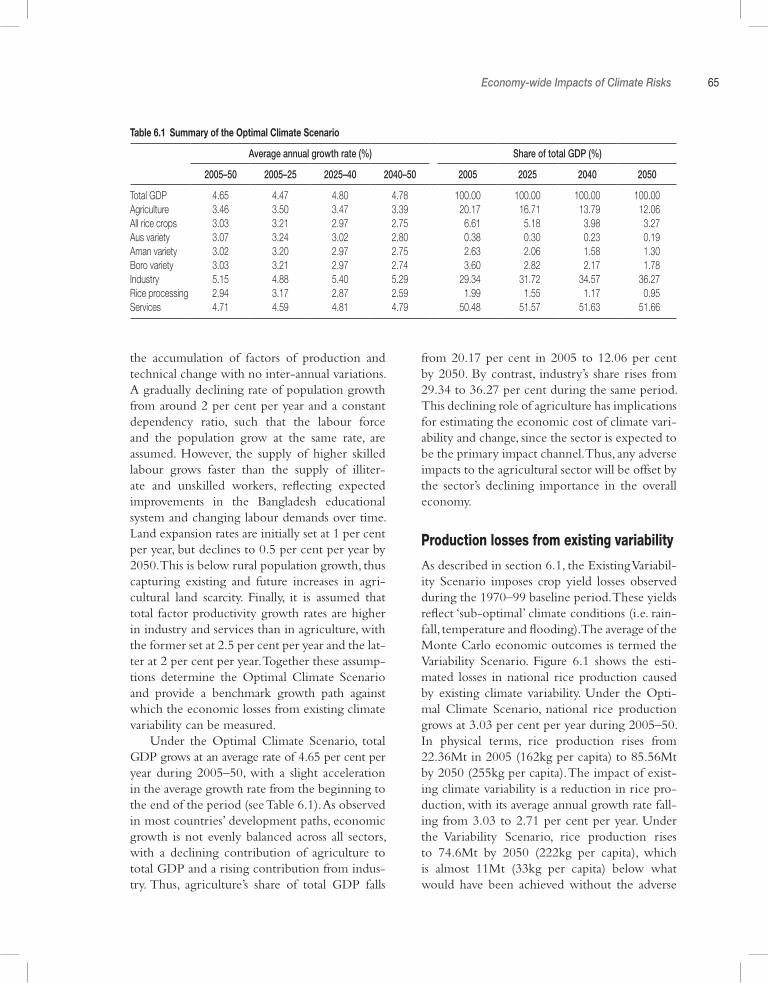
Economy-wide Impacts of Climate Risks 65
the accumulation of factors of production and technical change with no inter-annual variations. A gradually declining rate of population growth from around 2 per cent per year and a constant dependency ratio, such that the labour force and the population grow at the same rate, are assumed. However, the supply of higher skilled labour grows faster than the supply of illiter-ate and unskilled workers, reflecting expected improvements in the Bangladesh educational system and changing labour demands over time. Land expansion rates are initially set at 1 per cent per year, but declines to 0.5 per cent per year by 2050. This is below rural population growth, thus capturing existing and future increases in agri-cultural land scarcity. Finally, it is assumed that total factor productivity growth rates are higher in industry and services than in agriculture, with the former set at 2.5 per cent per year and the lat-ter at 2 per cent per year. Together these assump-tions determine the Optimal Climate Scenario and provide a benchmark growth path against which the economic losses from existing climate variability can be measured.
Under the Optimal Climate Scenario, total GDP grows at an average rate of 4.65 per cent per year during 2005–50, with a slight acceleration in the average growth rate from the beginning to the end of the period (see Table 6.1). As observed in most countries’ development paths, economic growth is not evenly balanced across all sectors, with a declining contribution of agriculture to total GDP and a rising contribution from indus-try. Thus, agriculture’s share of total GDP falls
from 20.17 per cent in 2005 to 12.06 per cent by 2050. By contrast, industry’s share rises from 29.34 to 36.27 per cent during the same period. This declining role of agriculture has implications for estimating the economic cost of climate vari-ability and change, since the sector is expected to be the primary impact channel. Thus, any adverse impacts to the agricultural sector will be offset by the sector’s declining importance in the overall economy.
Production losses from existing variability
As described in section 6.1, the Existing Variabil-ity Scenario imposes crop yield losses observed during the 1970–99 baseline period. These yields reflect ‘sub-optimal’ climate conditions (i.e. rain-fall, temperature and flooding). The average of the Monte Carlo economic outcomes is termed the Variability Scenario. Figure 6.1 shows the esti-mated losses in national rice production caused by existing climate variability. Under the Opti-mal Climate Scenario, national rice production grows at 3.03 per cent per year during 2005–50. In physical terms, rice production rises from 22.36Mt in 2005 (162kg per capita) to 85.56Mt by 2050 (255kg per capita). The impact of exist-ing climate variability is a reduction in rice pro-duction, with its average annual growth rate fall-ing from 3.03 to 2.71 per cent per year. Under the Variability Scenario, rice production rises to 74.6Mt by 2050 (222kg per capita), which is almost 11Mt (33kg per capita) below what would have been achieved without the adverse
Table 6.1 Summary of the Optimal Climate Scenario
Average annual growth rate (%) Share of total GDP (%)
2005–50 2005–25 2025–40 2040–50 2005 2025 2040 2050
Total GDP 4.65 4.47 4.80 4.78 100.00 100.00 100.00 100.00Agriculture 3.46 3.50 3.47 3.39 20.17 16.71 13.79 12.06All rice crops 3.03 3.21 2.97 2.75 6.61 5.18 3.98 3.27Aus variety 3.07 3.24 3.02 2.80 0.38 0.30 0.23 0.19Aman variety 3.02 3.20 2.97 2.75 2.63 2.06 1.58 1.30Boro variety 3.03 3.21 2.97 2.74 3.60 2.82 2.17 1.78Industry 5.15 4.88 5.40 5.29 29.34 31.72 34.57 36.27Rice processing 2.94 3.17 2.87 2.59 1.99 1.55 1.17 0.95Services 4.71 4.59 4.81 4.79 50.48 51.57 51.63 51.66
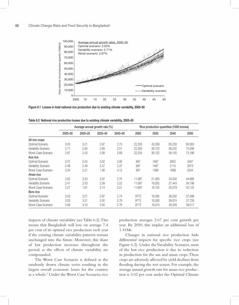
66 Climate Change Risks and Food Security in Bangladesh
impacts of climate variability (see Table 6.2). This means that Bangladesh will lose on average 7.4 per cent of its optimal rice production each year if the existing climate variability patterns remain unchanged into the future. Moreover, this share of lost production increases throughout the period, as the effects of climate variability are compounded.
The Worst Case Scenario is defined as the randomly drawn climate series resulting in the largest overall economic losses for the country as a whole.3 Under the Worst Case Scenario, rice
production averages 2.67 per cent growth per year. By 2050, this implies an additional loss of 1.41Mt.
Changes in national rice production hide differential impacts for specific rice crops (see Figure 6.2). Under the Variability Scenario, most of the lost rice production is due to reduction in production for the aus and aman crops. These crops are adversely affected by yield declines from flooding during the wet season. For example, the average annual growth rate for aman rice produc-tion is 3.02 per cent under the Optimal Climate
Figure 6.1 Losses in total national rice production due to existing climate variability, 2005–50
Table 6.2 National rice production losses due to existing climate variability, 2005–50
Average annual growth rate (%) Rice production quantities (1000 tonnes)
2005–50 2005–25 2025–40 2040–50 2005 2025 2040 2050
All rice cropsOptimal Scenario 3.03 3.21 2.97 2.75 22,355 42,038 65,226 85,563Variability Scenario 2.71 2.84 2.69 2.51 22,355 39,123 58,232 74,596Worst Case Scenario 2.67 2.43 2.98 2.69 22,355 36,122 56,105 73,186Aus riceOptimal Scenario 3.07 3.24 3.02 2.80 897 1697 2652 3497Variability Scenario 2.46 2.49 2.47 2.37 897 1467 2115 2673Worst Case Scenario 2.34 2.21 1.36 4.12 897 1388 1699 2544Aman riceOptimal Scenario 3.02 3.20 2.97 2.75 11,687 21,950 34,042 44,668Variability Scenario 2.41 2.53 2.39 2.22 11,687 19,262 27,443 34,196Worst Case Scenario 2.27 1.81 2.74 2.51 11,687 16,725 25,079 32,125Boro riceOptimal Scenario 3.03 3.21 2.97 2.74 9772 18,392 28,532 37,398Variability Scenario 3.05 3.21 3.00 2.78 9772 18,393 28,674 37,728Worst Case Scenario 3.09 3.10 3.30 2.76 9772 18,010 29,328 38,517
2005 10 15 20 25 30 35 40 45 50
100,000
90,000
80,000
70,000
60,000
50,000
40,000
30,000
20,000
10,000
0
Tota
l nat
iona
l ric
e p
rod
uctio
n q
uant
ity (1
000m
t) Average annual growth rates, 2005–50Optimal scenario: 3.03%Variability scenario: 2.71%Worst scenario: 2.67%
Optimal scenario
Variability scenario

Economy-wide Impacts of Climate Risks 67
Figure 6.2 Losses in national rice production by crop due to existing climate variability, 2005–50, (a) aus, (b) aman, (c) boro
Aus riceAverage annual growth rates, 2005–50Optimal scenario: 3.07%Variability scenario: 2.46%Worst scenario: 2.34%
Variability scenario
Optimal scenario
Optimal scenario
Variability scenario
Aman riceAverage annual growth rates, 2005–50Optimal scenario: 3.02%Variability scenario: 2.41%Worst scenario: 2.27%
4,000
3,500
3,000
2,500
2,000
1,500
1,000
500
0
Nat
iona
l Aus
ric
e p
rod
uctio
n q
uant
ity (1
000m
t)
2005 10 15 20 25 30 35 40 45 50
2005 10 15 20 25 30 35 40 45 50
2005 10 15 20 25 30 35 40 45 50
Optimal scenario
Variability scenario
Boro riceAverage annual growth rates, 2005–50Optimal scenario: 3.03%Variability scenario: 3.05%Worst scenario: 3.09%
Nat
iona
l Am
an r
ice
pro
duc
tion
qua
ntity
(100
0mt)
60,000
50,000
40,000
30,000
20,000
10,000
0
Nat
iona
l Bor
o ric
e p
rod
uctio
n q
uant
ity (1
000m
t)
45,000
40,000
35,000
30,000
25,000
20,000
15,000
10,000
5,000
0
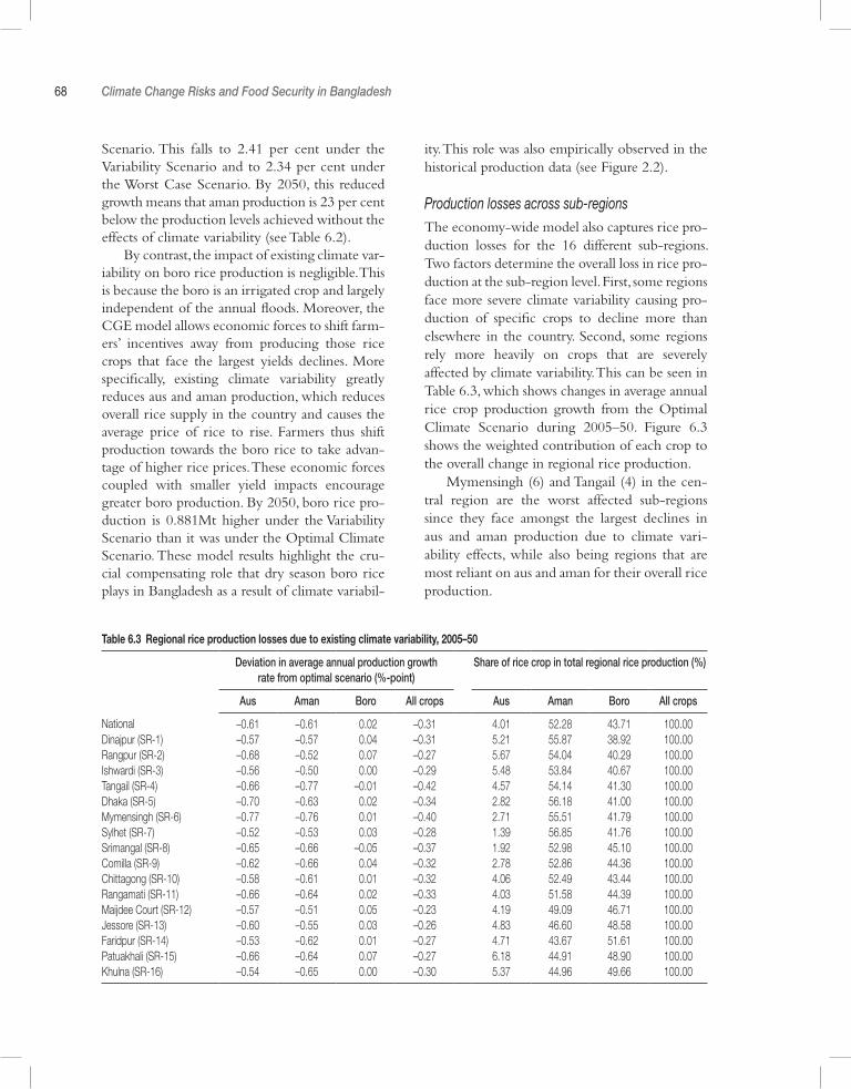
68 Climate Change Risks and Food Security in Bangladesh
Scenario. This falls to 2.41 per cent under the Variability Scenario and to 2.34 per cent under the Worst Case Scenario. By 2050, this reduced growth means that aman production is 23 per cent below the production levels achieved without the effects of climate variability (see Table 6.2).
By contrast, the impact of existing climate var-iability on boro rice production is negligible. This is because the boro is an irrigated crop and largely independent of the annual floods. Moreover, the CGE model allows economic forces to shift farm-ers’ incentives away from producing those rice crops that face the largest yields declines. More specifically, existing climate variability greatly reduces aus and aman production, which reduces overall rice supply in the country and causes the average price of rice to rise. Farmers thus shift production towards the boro rice to take advan-tage of higher rice prices. These economic forces coupled with smaller yield impacts encourage greater boro production. By 2050, boro rice pro-duction is 0.881Mt higher under the Variability Scenario than it was under the Optimal Climate Scenario. These model results highlight the cru-cial compensating role that dry season boro rice plays in Bangladesh as a result of climate variabil-
ity. This role was also empirically observed in the historical production data (see Figure 2.2).
Production losses across sub-regionsThe economy-wide model also captures rice pro-duction losses for the 16 different sub-regions. Two factors determine the overall loss in rice pro-duction at the sub-region level. First, some regions face more severe climate variability causing pro-duction of specific crops to decline more than elsewhere in the country. Second, some regions rely more heavily on crops that are severely affected by climate variability. This can be seen in Table 6.3, which shows changes in average annual rice crop production growth from the Optimal Climate Scenario during 2005–50. Figure 6.3 shows the weighted contribution of each crop to the overall change in regional rice production.
Mymensingh (6) and Tangail (4) in the cen-tral region are the worst affected sub-regions since they face amongst the largest declines in aus and aman production due to climate vari-ability effects, while also being regions that are most reliant on aus and aman for their overall rice production.
Table 6.3 Regional rice production losses due to existing climate variability, 2005–50
Deviation in average annual production growth rate from optimal scenario (%-point)
Share of rice crop in total regional rice production (%)
Aus Aman Boro All crops Aus Aman Boro All crops
National –0.61 –0.61 –0.02 –0.31 4.01 52.28 43.71 100.00Dinajpur (SR-1) –0.57 –0.57 –0.04 –0.31 5.21 55.87 38.92 100.00Rangpur (SR-2) –0.68 –0.52 –0.07 –0.27 5.67 54.04 40.29 100.00Ishwardi (SR-3) –0.56 –0.50 –0.00 –0.29 5.48 53.84 40.67 100.00Tangail (SR-4) –0.66 –0.77 –0.01 –0.42 4.57 54.14 41.30 100.00Dhaka (SR-5) –0.70 –0.63 –0.02 –0.34 2.82 56.18 41.00 100.00Mymensingh (SR-6) –0.77 –0.76 –0.01 –0.40 2.71 55.51 41.79 100.00Sylhet (SR-7) –0.52 –0.53 –0.03 –0.28 1.39 56.85 41.76 100.00Srimangal (SR-8) –0.65 –0.66 –0.05 –0.37 1.92 52.98 45.10 100.00Comilla (SR-9) –0.62 –0.66 –0.04 –0.32 2.78 52.86 44.36 100.00Chittagong (SR-10) –0.58 –0.61 –0.01 –0.32 4.06 52.49 43.44 100.00Rangamati (SR-11) –0.66 –0.64 –0.02 –0.33 4.03 51.58 44.39 100.00Maijdee Court (SR-12) –0.57 –0.51 –0.05 –0.23 4.19 49.09 46.71 100.00Jessore (SR-13) –0.60 –0.55 –0.03 –0.26 4.83 46.60 48.58 100.00Faridpur (SR-14) –0.53 –0.62 –0.01 –0.27 4.71 43.67 51.61 100.00Patuakhali (SR-15) –0.66 –0.64 –0.07 –0.27 6.18 44.91 48.90 100.00Khulna (SR-16) –0.54 –0.65 –0.00 –0.30 5.37 44.96 49.66 100.00
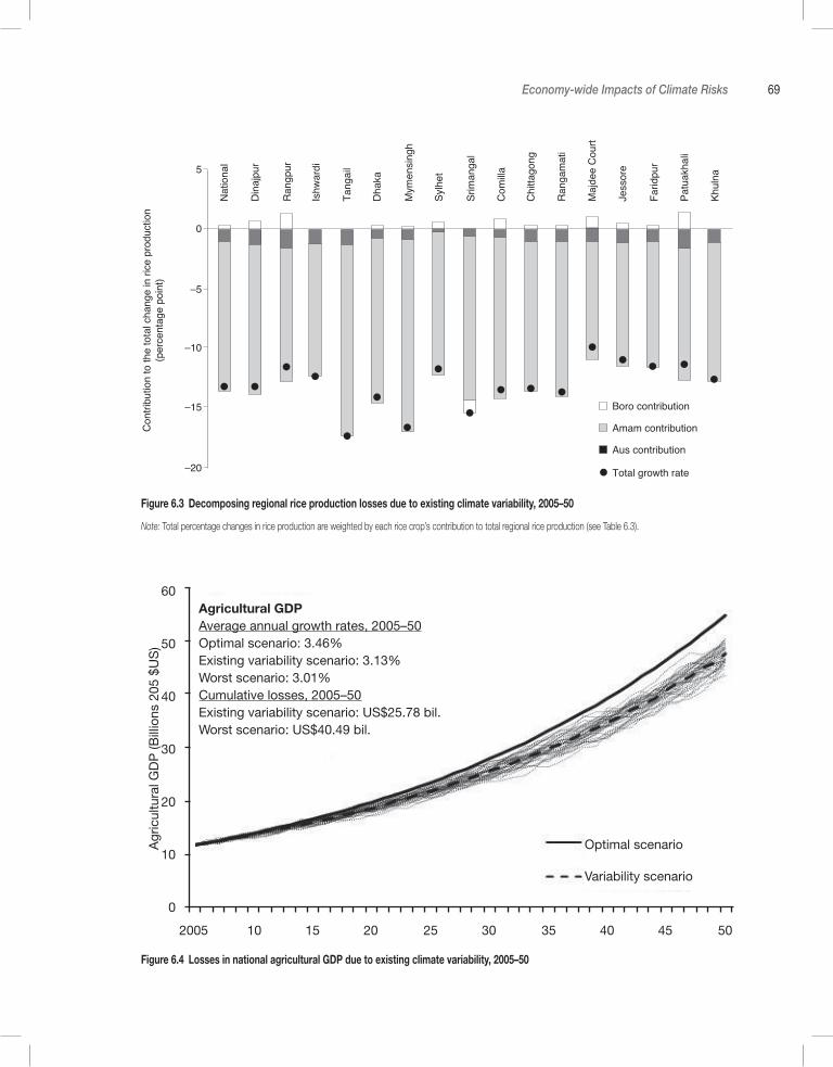
Economy-wide Impacts of Climate Risks 69
Figure 6.3 Decomposing regional rice production losses due to existing climate variability, 2005–50
Note: Total percentage changes in rice production are weighted by each rice crop’s contribution to total regional rice production (see Table 6.3).
Figure 6.4 Losses in national agricultural GDP due to existing climate variability, 2005–50
National
Din
ajp
ur
Rangpur
Ishw
ard
i
Tangail
Dhaka
Mym
ensin
gh
Sylh
et
Srim
angal
Com
illa
Chitta
gong
Rangam
ati
Majd
ee C
our t
Jessore
Faridpur
Patu
akhal i
Khuln
a
Contr
ibution to the tota
l change in r
ice p
roductio
n(p
erc
enta
ge p
oin
t)
Boro contribution
Amam contribution
Aus contribution
Total growth rate–20
–15
–10
–5
0
5
60
50
40
30
20
10
0
Agr
icul
tura
l GD
P (B
illio
ns 2
05 $
US
)
Agricultural GDPAverage annual growth rates, 2005–50Optimal scenario: 3.46%Existing variability scenario: 3.13%Worst scenario: 3.01%Cumulative losses, 2005–50Existing variability scenario: US$25.78 bil.Worst scenario: US$40.49 bil.
Optimal scenario
Variability scenario
2005 10 15 20 25 30 35 40 45 50
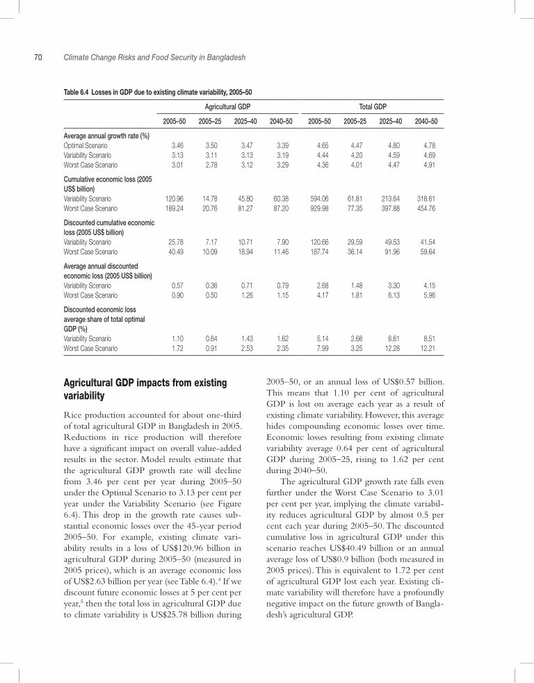
70 Climate Change Risks and Food Security in Bangladesh
Table 6.4 Losses in GDP due to existing climate variability, 2005–50
Agricultural GDP Total GDP
2005–50 2005–25 2025–40 2040–50 2005–50 2005–25 2025–40 2040–50
Average annual growth rate (%)Optimal Scenario 3.46 3.50 3.47 3.39 4.65 4.47 4.80 4.78Variability Scenario 3.13 3.11 3.13 3.19 4.44 4.20 4.59 4.69Worst Case Scenario 3.01 2.78 3.12 3.29 4.36 4.01 4.47 4.91
Cumulative economic loss (2005 US$ billion)Variability Scenario 120.96 14.78 45.80 60.38 594.06 61.81 213.64 318.61Worst Case Scenario 189.24 20.76 81.27 87.20 929.98 77.35 397.88 454.76
Discounted cumulative economic loss (2005 US$ billion)Variability Scenario 25.78 7.17 10.71 7.90 120.66 29.59 49.53 41.54Worst Case Scenario 40.49 10.09 18.94 11.46 187.74 36.14 91.96 59.64
Average annual discounted economic loss (2005 US$ billion)Variability Scenario 0.57 0.36 0.71 0.79 2.68 1.48 3.30 4.15Worst Case Scenario 0.90 0.50 1.26 1.15 4.17 1.81 6.13 5.96
Discounted economic loss average share of total optimal GDP (%)Variability Scenario 1.10 0.64 1.43 1.62 5.14 2.66 6.61 8.51Worst Case Scenario 1.72 0.91 2.53 2.35 7.99 3.25 12.28 12.21
Agricultural GDP impacts from existing variability
Rice production accounted for about one-third of total agricultural GDP in Bangladesh in 2005. Reductions in rice production will therefore have a significant impact on overall value-added results in the sector. Model results estimate that the agricultural GDP growth rate will decline from 3.46 per cent per year during 2005–50 under the Optimal Scenario to 3.13 per cent per year under the Variability Scenario (see Figure 6.4). This drop in the growth rate causes sub-stantial economic losses over the 45-year period 2005–50. For example, existing climate vari-ability results in a loss of US$120.96 billion in agricultural GDP during 2005–50 (measured in 2005 prices), which is an average economic loss of US$2.63 billion per year (see Table 6.4).4 If we discount future economic losses at 5 per cent per year,5 then the total loss in agricultural GDP due to climate variability is US$25.78 billion during
2005–50, or an annual loss of US$0.57 billion. This means that 1.10 per cent of agricultural GDP is lost on average each year as a result of existing climate variability. However, this average hides compounding economic losses over time. Economic losses resulting from existing climate variability average 0.64 per cent of agricultural GDP during 2005–25, rising to 1.62 per cent during 2040–50.
The agricultural GDP growth rate falls even further under the Worst Case Scenario to 3.01 per cent per year, implying the climate variabil-ity reduces agricultural GDP by almost 0.5 per cent each year during 2005–50. The discounted cumulative loss in agricultural GDP under this scenario reaches US$40.49 billion or an annual average loss of US$0.9 billion (both measured in 2005 prices). This is equivalent to 1.72 per cent of agricultural GDP lost each year. Existing cli-mate variability will therefore have a profoundly negative impact on the future growth of Bangla-desh’s agricultural GDP.
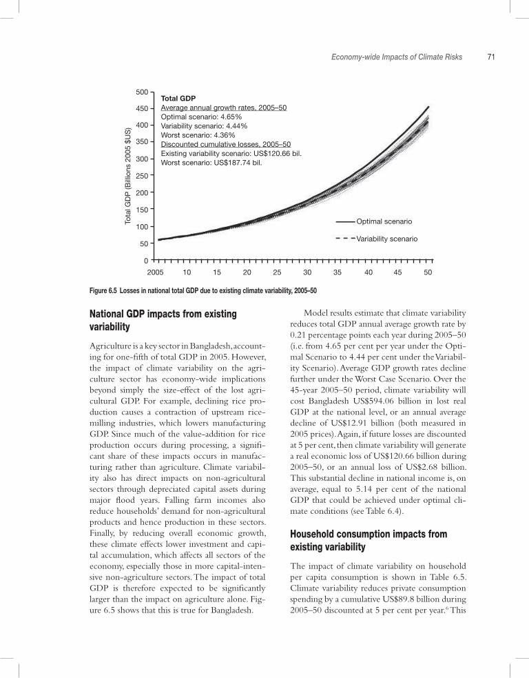
Economy-wide Impacts of Climate Risks 71
National GDP impacts from existing variability
Agriculture is a key sector in Bangladesh, account-ing for one-fifth of total GDP in 2005. However, the impact of climate variability on the agri-culture sector has economy-wide implications beyond simply the size-effect of the lost agri-cultural GDP. For example, declining rice pro-duction causes a contraction of upstream rice-milling industries, which lowers manufacturing GDP. Since much of the value-addition for rice production occurs during processing, a signifi-cant share of these impacts occurs in manufac-turing rather than agriculture. Climate variabil-ity also has direct impacts on non-agricultural sectors through depreciated capital assets during major flood years. Falling farm incomes also reduce households’ demand for non-agricultural products and hence production in these sectors. Finally, by reducing overall economic growth, these climate effects lower investment and capi-tal accumulation, which affects all sectors of the economy, especially those in more capital-inten-sive non-agriculture sectors. The impact of total GDP is therefore expected to be significantly larger than the impact on agriculture alone. Fig-ure 6.5 shows that this is true for Bangladesh.
Model results estimate that climate variability reduces total GDP annual average growth rate by 0.21 percentage points each year during 2005–50 (i.e. from 4.65 per cent per year under the Opti-mal Scenario to 4.44 per cent under the Variabil-ity Scenario). Average GDP growth rates decline further under the Worst Case Scenario. Over the 45-year 2005–50 period, climate variability will cost Bangladesh US$594.06 billion in lost real GDP at the national level, or an annual average decline of US$12.91 billion (both measured in 2005 prices). Again, if future losses are discounted at 5 per cent, then climate variability will generate a real economic loss of US$120.66 billion during 2005–50, or an annual loss of US$2.68 billion. This substantial decline in national income is, on average, equal to 5.14 per cent of the national GDP that could be achieved under optimal cli-mate conditions (see Table 6.4).
Household consumption impacts from existing variability
The impact of climate variability on household per capita consumption is shown in Table 6.5. Climate variability reduces private consumption spending by a cumulative US$89.8 billion during 2005–50 discounted at 5 per cent per year.6 This
Figure 6.5 Losses in national total GDP due to existing climate variability, 2005–50
Total GDPAverage annual growth rates, 2005–50Optimal scenario: 4.65%Variability scenario: 4.44%Worst scenario: 4.36%Discounted cumulative losses, 2005–50Existing variability scenario: US$120.66 bil.Worst scenario: US$187.74 bil.
500
450
400
350
300
250
200
150
100
50
0
Tota
l GD
P (B
illio
ns 2
005
$US
)
Optimal scenario
Variability scenario
2005 10 15 20 25 30 35 40 45 50
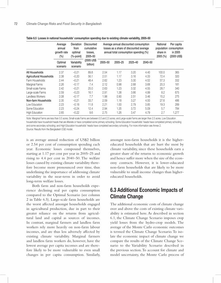
72 Climate Change Risks and Food Security in Bangladesh
is an average annual reduction of US$2 billion or 2.54 per cent of consumption spending each year. Economic losses compound themselves, starting at 1.17 per cent per year in 2005–25 and rising to 4.4 per cent in 2040–50. The welfare losses caused by existing climate variability there-fore become more pronounced over time, thus underlining the importance of addressing climate variability in the near-term in order to avoid long-term welfare losses.
Both farm and non-farm households expe-rience declining real per capita consumption compared to the Optimal Scenario (see column 2 in Table 6.5). Large-scale farm households are the worst affected amongst households engaged in agricultural production, due in part to their greater reliance on the returns from agricul-tural land and capital as sources of incomes. In contrast, marginal farmers and landless farm workers rely more heavily on non-farm labour incomes, and are thus less adversely affected by existing climate variability. Marginal farmers and landless farm workers do, however, have the lowest average per capita incomes and are there-fore likely to be more vulnerable to even small changes in per capita consumption. Similarly,
amongst non-farm households it is the higher-educated households that are hurt the most by climate variability, since these households earn a greater share of the returns to economic growth and hence suffer more when the size of the econ-omy contracts. However, it is lower-educated non-farm households that are likely to be more vulnerable to small income changes than higher-educated households.
6.3 Additional Economic Impacts of Climate ChangeThe additional economic costs of climate change over and above the costs of existing climate vari-ability is estimated here. As described in section 6.1, the Climate Change Scenario imposes crop yield losses from the hydro-crop models. The average of the Monte Carlo economic outcomes is termed the Climate Change Scenario. To iso-late the economic impact of climate change we compare the results of the Climate Change Sce-nario to the Variability Scenario described in the previous section. To account for climate and model uncertainty, the Monte Carlo process of
Table 6.5 Losses in national households’ consumption spending due to existing climate variability, 2005–50
Average annual
growth rate (%)
Deviation from
optimal (%-point)
Discounted cumulative
losses, 2005–50
(2005 US$ billion)
Average annual discounted consumption losses as a share of discounted average annual total consumption spending (%)
National population
share in 2005 (%)
Per capita consumption
in 2005 (2005 US$)
Optimal scenario
Variability scenario
2005–50 2005–25 2025–40 2040–50
All Households 2.37 –0.21 89.8 2.54 1.17 3.20 4.40 100.0 ,365Agricultural Households 2.38 –0.20 56.1 2.51 1.17 3.16 4.33 72.4 ,320Farm Households 2.44 –0.21 48.4 2.62 1.23 3.30 4.52 57.3 ,332Marginal Farms 2.26 –0.17 7.4 2.12 0.98 2.68 3.68 20.3 ,181Small-scale Farms 2.42 –0.21 25.0 2.63 1.23 3.32 4.55 28.7 ,340Large-scale Farms 2.59 –0.23 16.1 2.91 1.38 3.66 4.99 8.2 ,675Landless Workers 2.08 –0.17 7.7 1.98 0.90 2.51 3.46 15.2 ,275Non-farm Households 2.35 –0.21 33.7 2.59 1.18 3.27 4.50 27.6 ,486Low Education 2.23 –0.18 11.8 2.21 1.00 2.79 3.85 19.3 ,289Some Education 2.23 –0.24 12.4 2.94 1.35 3.72 5.09 5.7 ,784High Education 2.65 –0.22 9.6 2.75 1.26 3.47 4.79 2.7 1,277
Note: Marginal Farms are less than 0.5 acres; Small-scale Farms are between 0.5 and 2.5 acres; and Large-scale Farms are larger than 2.5 acres. Low Education households have household heads that are illiterate or have completed some primary schooling; Some Education households’ heads have completed primary schooling and some secondary schooling; and High Education households’ heads have completed secondary schooling. For more information see Annex 2. Source: Results from the Bangladesh CGE model.
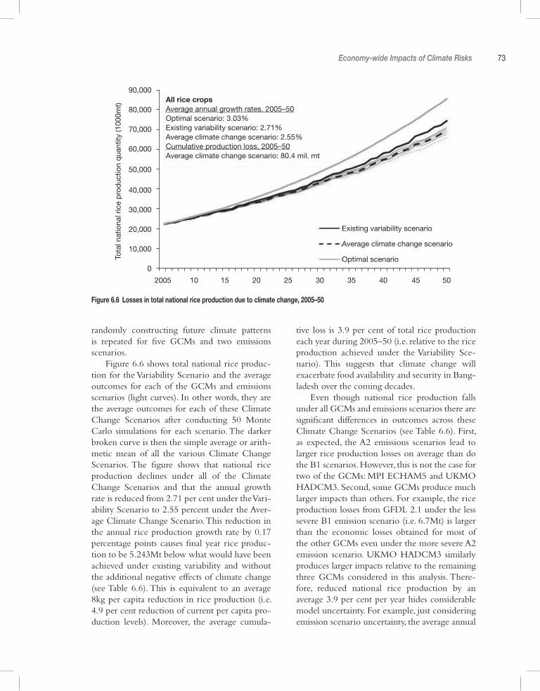
Economy-wide Impacts of Climate Risks 73
randomly constructing future climate patterns is repeated for five GCMs and two emissions scenarios.
Figure 6.6 shows total national rice produc-tion for the Variability Scenario and the average outcomes for each of the GCMs and emissions scenarios (light curves). In other words, they are the average outcomes for each of these Climate Change Scenarios after conducting 50 Monte Carlo simulations for each scenario. The darker broken curve is then the simple average or arith-metic mean of all the various Climate Change Scenarios. The figure shows that national rice production declines under all of the Climate Change Scenarios and that the annual growth rate is reduced from 2.71 per cent under the Vari-ability Scenario to 2.55 percent under the Aver-age Climate Change Scenario. This reduction in the annual rice production growth rate by 0.17 percentage points causes final year rice produc-tion to be 5.243Mt below what would have been achieved under existing variability and without the additional negative effects of climate change (see Table 6.6). This is equivalent to an average 8kg per capita reduction in rice production (i.e. 4.9 per cent reduction of current per capita pro-duction levels). Moreover, the average cumula-
tive loss is 3.9 per cent of total rice production each year during 2005–50 (i.e. relative to the rice production achieved under the Variability Sce-nario). This suggests that climate change will exacerbate food availability and security in Bang-ladesh over the coming decades.
Even though national rice production falls under all GCMs and emissions scenarios there are significant differences in outcomes across these Climate Change Scenarios (see Table 6.6). First, as expected, the A2 emissions scenarios lead to larger rice production losses on average than do the B1 scenarios. However, this is not the case for two of the GCMs: MPI ECHAM5 and UKMO HADCM3. Second, some GCMs produce much larger impacts than others. For example, the rice production losses from GFDL 2.1 under the less severe B1 emission scenario (i.e. 6.7Mt) is larger than the economic losses obtained for most of the other GCMs even under the more severe A2 emission scenario. UKMO HADCM3 similarly produces larger impacts relative to the remaining three GCMs considered in this analysis. There-fore, reduced national rice production by an average 3.9 per cent per year hides considerable model uncertainty. For example, just considering emission scenario uncertainty, the average annual
Figure 6.6 Losses in total national rice production due to climate change, 2005–50
All rice cropsAverage annual growth rates, 2005–50Optimal scenario: 3.03%Existing variability scenario: 2.71%Average climate change scenario: 2.55%Cumulative production loss, 2005–50Average climate change scenario: 80.4 mil. mt
Existing variability scenario
Average climate change scenario
Optimal scenario
90,000
80,000
70,000
60,000
50,000
40,000
30,000
20,000
10,000
0
Tota
l nat
iona
l ric
e p
rod
uctio
n q
uant
ity (1
000m
t)
2005 10 15 20 25 30 35 40 45 50
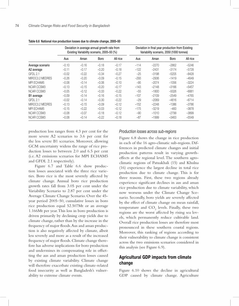
74 Climate Change Risks and Food Security in Bangladesh
Table 6.6 National rice production losses due to climate change, 2005–50
Deviation in average annual growth rate from Existing Variability scenario, 2005–50 (%)
Deviation in final year production from Existing Variability scenario, 2050 (1000 tonnes)
Aus Aman Boro All rice Aus Aman Boro All rice
Average scenario –0.10 –0.16 –0.18 –0.17 –114 –2270 –2862 –5246A2 average –0.11 –0.17 –0.20 –0.18 –122 –2431 –3174 –5728GFDL 2.1 –0.02 –0.22 –0.34 –0.27 –25 –3198 –5205 –8428MIROC3.2 MEDRES –0.26 –0.20 –0.09 –0.15 –293 –2936 –1419 –4649MPI ECHAM5 –0.08 –0.14 –0.06 –0.10 –95 –2074 –1056 –3224NCAR CCSM3 –0.13 –0.15 –0.20 –0.17 –143 –2148 –3166 –5457NCAR CCSM3 –0.05 –0.12 –0.33 –0.22 –55 –1800 –5026 –6881B1 average –0.09 –0.14 –0.16 –0.15 –107 –2109 –2549 –4765GFDL 2.1 –0.02 –0.14 –0.30 –0.22 –29 –2069 –4616 –6714MIROC3.2 MEDRES –0.13 –0.15 –0.09 –0.12 –152 –2248 –1386 –3786MPI ECHAM5 –0.15 –0.22 –0.03 –0.12 –175 –3219 –483 –3878NCAR CCSM3 –0.08 –0.07 –0.18 –0.12 –90 –1010 –2799 –3899NCAR CCSM3 –0.08 –0.14 –0.22 –0.18 –87 –1999 –3463 –5549
production loss ranges from 4.3 per cent for the more severe A2 scenarios to 3.6 per cent for the less severe B1 scenarios. Moreover, allowing GCM uncertainty widens the range of rice pro-duction losses to between 2.0 and 6.5 per cent (i.e. A2 emissions scenarios for MPI ECHAM5 and GFDL 2.1 respectively).
Figure 6.7 and Table 6.6 show produc-tion losses associated with the three rice varie-ties. Boro rice is the most severely affected by climate change. Annual boro rice production growth rates fall from 3.05 per cent under the Variability Scenario to 2.87 per cent under the Average Climate Change Scenario. Over the 45-year period 2005–50, cumulative losses in boro rice production equal 52.507Mt or an average 1.166Mt per year. This loss in boro production is driven primarily by declining crop yields due to climate change, rather than by the increase in the frequency of major floods. Aus and aman produc-tion is also negatively affected by climate, albeit less severely and more as a result of the increased frequency of major floods. Climate change there-fore has adverse implications for boro production and undermines its compensating role in offset-ting the aus and aman production losses caused by existing climate variability. Climate change will therefore exacerbate existing climate-related food insecurity as well as Bangladesh’s vulner-ability to extreme climate events.
Production losses across sub-regionsFigure 6.8 shows the change in rice production in each of the 16 agro-climatic sub-regions. Dif-ferences in predicted climate changes and initial production patterns result in varying growth-effects at the regional level. The southern agro-climatic regions of Patuakhali (15) and Khulna (16) experience the largest decline in total rice production due to climate change. This is for three reasons. First, these two regions already experience significant declines in aus and aman rice production due to climate variability, which now worsens under the Climate Change Sce-nario. Secondly, boro yields are severely affected by the effect of climate change on mean rainfall, temperature and CO
2 levels. Finally, these two
regions are the worst affected by rising sea lev-els, which permanently reduce cultivable land. Overall rice production losses are therefore most pronounced in these southern coastal regions. Moreover, this ranking of regions according to their vulnerability to climate change is consistent across the two emissions scenarios considered in this analysis (see Figure 6.9).
Agricultural GDP impacts from climate changeFigure 6.10 shows the decline in agricultural GDP caused by climate change. Agriculture
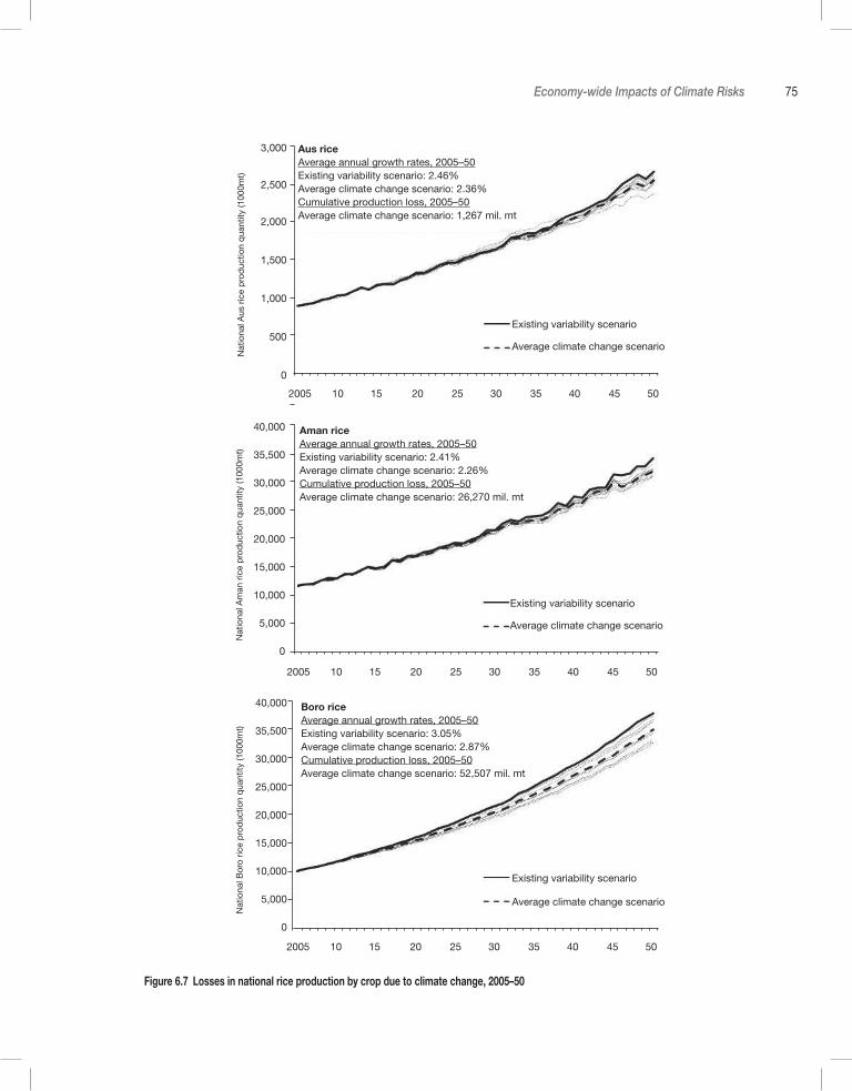
Economy-wide Impacts of Climate Risks 75
Figure 6.7 Losses in national rice production by crop due to climate change, 2005–50
Aus riceAverage annual growth rates, 2005–50Existing variability scenario: 2.46%Average climate change scenario: 2.36%Cumulative production loss, 2005–50Average climate change scenario: 1,267 mil. mt
Existing variability scenario
Average climate change scenario
3,000
2,500
2,000
1,500
1,000
500
0
Nat
iona
l Aus
ric
e p
rod
uctio
n q
uant
ity (1
000m
t)
2005 10 15 20 25 30 35 40 45 50
Aman riceAverage annual growth rates, 2005–50Existing variability scenario: 2.41%Average climate change scenario: 2.26%Cumulative production loss, 2005–50Average climate change scenario: 26,270 mil. mt
Existing variability scenario
Average climate change scenario
40,000
35,500
30,000
25,000
20,000
15,000
10,000
5,000
0
2005 10 15 20 25 30 35 40 45 50
Nat
iona
l Am
an r
ice
pro
duc
tion
qua
ntity
(100
0mt)
Existing variability scenario
Average climate change scenario
Boro riceAverage annual growth rates, 2005–50Existing variability scenario: 3.05%Average climate change scenario: 2.87%Cumulative production loss, 2005–50Average climate change scenario: 52,507 mil. mt
2005 10 15 20 25 30 35 40 45 50
40,000
35,500
30,000
25,000
20,000
15,000
10,000
5,000
0
Nat
iona
l Bor
o ric
e p
rod
uctio
n q
uant
ity (1
000m
t)
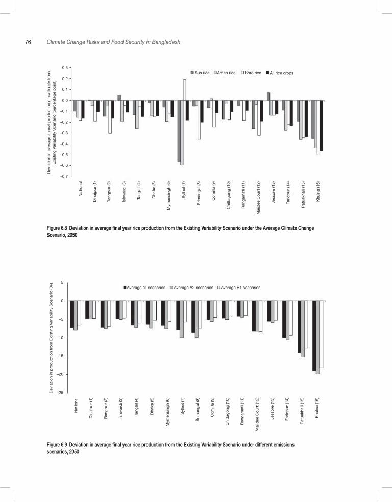
76 Climate Change Risks and Food Security in Bangladesh
Figure 6.9 Deviation in average final year rice production from the Existing Variability Scenario under different emissions scenarios, 2050
Figure 6.8 Deviation in average final year rice production from the Existing Variability Scenario under the Average Climate Change Scenario, 2050
Aus rice Aman rice Boro rice All rice crops0.3
0.2
0.1
0.0
–0.1
–0.2
–0.3
–0.4
–0.5
–0.6
–0.7
Dev
iatio
n in
ave
rage
ann
ual p
rod
uctio
n gr
owth
rat
e fr
om
Exi
stin
g Va
riab
ility
Sce
nario
(per
cent
age
poi
nt)
Nat
iona
l
Din
ajp
ur (1
)
Ran
gpur
(2)
Ishw
ard
i (3)
Tang
ail (
4)
Dha
ka (5
)
Mym
ensi
ngh
(6)
Syl
het
(7)
Srim
anga
l (8)
Com
illa
(9)
Chi
ttag
ong
(10)
Ran
gam
ati (
11)
Mai
jdee
Cou
rt (1
2)
Jess
ore
(13)
Farid
pur
(14)
Pat
uakh
ali (
15)
Khu
lna
(16)
Nat
iona
l
Din
ajp
ur (1
)
Ran
gpur
(2)
Ishw
ard
i (3)
Tang
ail (
4)
Dha
ka (5
)
Mym
ensi
ngh
(6)
Syl
het
(7)
Srim
anga
l (8)
Com
illa
(9)
Chi
ttag
ong
(10)
Ran
gam
ati (
11)
Mai
jdee
Cou
rt (1
2)
Jess
ore
(13)
Farid
pur
(14)
Pat
uakh
ali (
15)
Khu
lna
(16)
Dev
iatio
n in
pro
duc
tion
from
Exi
stin
g Va
riab
ility
Sce
nario
(%) 5
0
–5
–10
–15
–20
–25
Average all scenarios Average A2 scenarios Average B1 scenarios
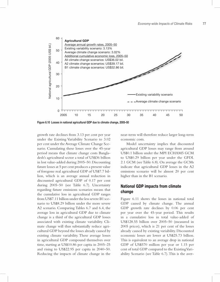
Economy-wide Impacts of Climate Risks 77
growth rate declines from 3.13 per cent per year under the Existing Variability Scenario to 3.02 per cent under the Average Climate Change Sce-nario. Cumulating these losses over the 45-year period means that climate change costs Bangla-desh’s agricultural sector a total of US$36 billion in lost value-added during 2005–50. Discounting future losses at 5 per cent produces a present value of foregone real agricultural GDP of US$7.7 bil-lion, which is an average annual reduction in discounted agricultural GDP of 0.17 per cent during 2005–50 (see Table 6.7). Uncertainty regarding future emissions scenarios means that the cumulative loss in agricultural GDP ranges from US$7.11 billion under the less severe B1 sce-nario to US$8.29 billion under the more severe A2 scenario. Comparing Tables 6.7 and 6.4, the average loss in agricultural GDP due to climate change is a third of the agricultural GDP losses associated with existing climate variability. Cli-mate change will thus substantially reduce agri-cultural GDP beyond the losses already caused by existing climate variability. These average losses in agricultural GDP compound themselves over time, starting at US$10.86 per capita in 2005–25 and rising to US$22.95 per capita in 2040–50. Reducing the impacts of climate change in the
Figure 6.10 Losses in national agricultural GDP due to climate change, 2005–50
near-term will therefore reduce larger long-term economic costs.
Model uncertainty implies that discounted agricultural GDP losses may range from around US$0.1 billion under the MPI ECHAM5 GCM to US$0.29 billion per year under the GFDL 2.1 GCM (see Table 6.8). On average the GCMs indicate that agricultural GDP losses in the A2 emissions scenario will be almost 20 per cent higher than in the B1 scenario.
National GDP impacts from climate change
Figure 6.11 shows the losses in national total GDP caused by climate change. The annual GDP growth rate declines by 0.06 per cent per year over the 45-year period. This results in a cumulative loss in total value-added of US$128.55 billion over 2005–50 (measured in 2005 prices), which is 21 per cent of the losses already caused by existing variability. Discounted economic losses are lower at US$25.73 billion. This is equivalent to an average drop in national GDP of US$570 million per year or 1.15 per cent of total GDP compared to the Existing Vari-ability Scenario (see Table 6.7). This is the aver-
Agricultural GDPAverage annual growth rates, 2005–50Existing variability scenario: 3.13%Average climate change scenario: 3.02%Additional cumulative economic loss, 2005–50All climate change scenarios: US$36.02 bil.A2 climate change scenarios: US$39.17 bil.B1 climate change scenarios: US$32.86 bil.
Existing variability scenario
Average climate change scenario
2005 10 15 20 25 30 35 40 45 50
60
50
40
30
20
10
0
Nat
iona
l agr
icul
tura
l GD
P (2
005
US
$ b
il.)
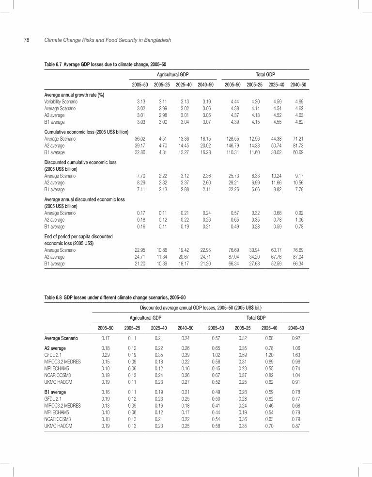
78 Climate Change Risks and Food Security in Bangladesh
Table 6.7 Average GDP losses due to climate change, 2005–50
Agricultural GDP Total GDP
2005–50 2005–25 2025–40 2040–50 2005–50 2005–25 2025–40 2040–50
Average annual growth rate (%)Variability Scenario 3.13 3.11 3.13 3.19 4.44 4.20 4.59 4.69Average Scenario 3.02 2.99 3.02 3.06 4.38 4.14 4.54 4.62A2 average 3.01 2.98 3.01 3.05 4.37 4.13 4.52 4.63B1 average 3.03 3.00 3.04 3.07 4.39 4.15 4.55 4.62
Cumulative economic loss (2005 US$ billion)Average Scenario 36.02 4.51 13.36 18.15 128.55 12.96 44.38 71.21A2 average 39.17 4.70 14.45 20.02 146.79 14.33 50.74 81.73B1 average 32.86 4.31 12.27 16.28 110.31 11.60 38.02 60.69
Discounted cumulative economic loss (2005 US$ billion)Average Scenario 7.70 2.22 3.12 2.36 25.73 6.33 10.24 9.17A2 average 8.29 2.32 3.37 2.60 29.21 6.99 11.66 10.56B1 average 7.11 2.13 2.88 2.11 22.26 5.66 8.82 7.78
Average annual discounted economic loss (2005 US$ billion)Average Scenario 0.17 0.11 0.21 0.24 0.57 0.32 0.68 0.92A2 average 0.18 0.12 0.22 0.26 0.65 0.35 0.78 1.06B1 average 0.16 0.11 0.19 0.21 0.49 0.28 0.59 0.78
End of period per capita discounted economic loss (2005 US$)Average Scenario 22.95 10.86 19.42 22.95 76.69 30.94 60.17 76.69A2 average 24.71 11.34 20.67 24.71 87.04 34.20 67.76 87.04B1 average 21.20 10.39 18.17 21.20 66.34 27.68 52.59 66.34
Table 6.8 GDP losses under different climate change scenarios, 2005–50
Discounted average annual GDP losses, 2005–50 (2005 US$ bil.)
Agricultural GDP Total GDP
2005–50 2005–25 2025–40 2040–50 2005–50 2005–25 2025–40 2040–50
Average Scenario 0.17 0.11 0.21 0.24 0.57 0.32 0.68 0.92
A2 average 0.18 0.12 0.22 0.26 0.65 0.35 0.78 1.06GFDL 2.1 0.29 0.19 0.35 0.39 1.02 0.59 1.20 1.63MIROC3.2 MEDRES 0.15 0.09 0.18 0.22 0.58 0.31 0.69 0.96MPI ECHAM5 0.10 0.06 0.12 0.16 0.45 0.23 0.55 0.74NCAR CCSM3 0.19 0.13 0.24 0.26 0.67 0.37 0.82 1.04UKMO HADCM 0.19 0.11 0.23 0.27 0.52 0.25 0.62 0.91
B1 average 0.16 0.11 0.19 0.21 0.49 0.28 0.59 0.78GFDL 2.1 0.19 0.12 0.23 0.25 0.50 0.28 0.62 0.77MIROC3.2 MEDRES 0.13 0.09 0.16 0.18 0.41 0.24 0.46 0.68MPI ECHAM5 0.10 0.06 0.12 0.17 0.44 0.19 0.54 0.79NCAR CCSM3 0.18 0.13 0.21 0.22 0.54 0.36 0.63 0.79UKMO HADCM 0.19 0.13 0.23 0.25 0.58 0.35 0.70 0.87
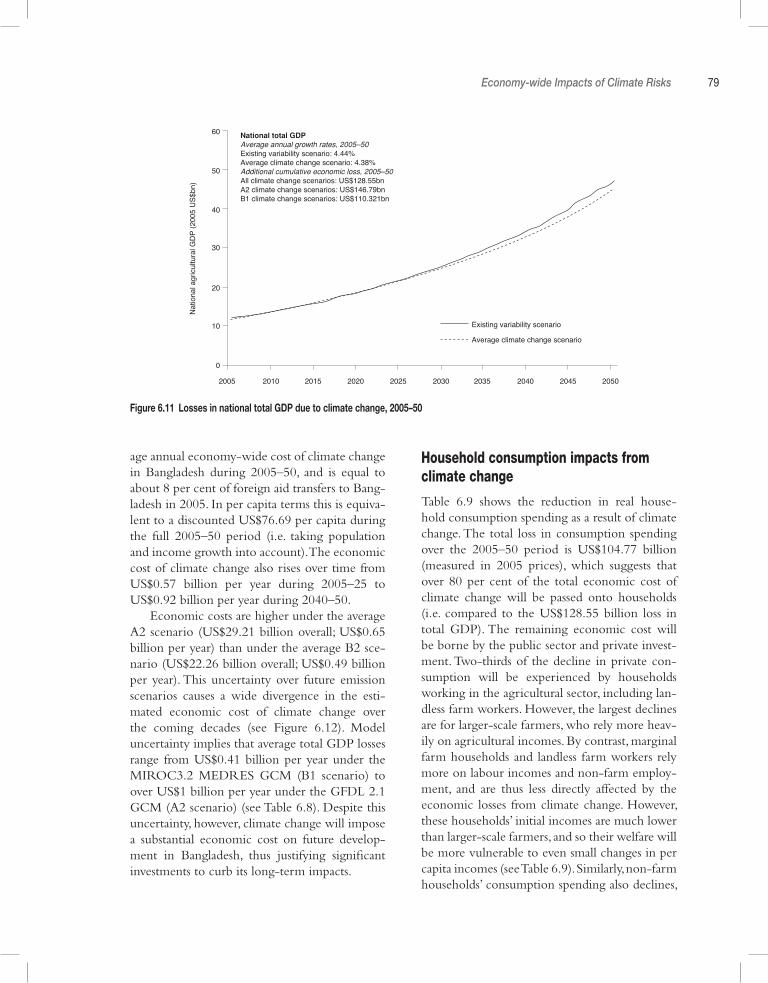
Economy-wide Impacts of Climate Risks 79
age annual economy-wide cost of climate change in Bangladesh during 2005–50, and is equal to about 8 per cent of foreign aid transfers to Bang-ladesh in 2005. In per capita terms this is equiva-lent to a discounted US$76.69 per capita during the full 2005–50 period (i.e. taking population and income growth into account). The economic cost of climate change also rises over time from US$0.57 billion per year during 2005–25 to US$0.92 billion per year during 2040–50.
Economic costs are higher under the average A2 scenario (US$29.21 billion overall; US$0.65 billion per year) than under the average B2 sce-nario (US$22.26 billion overall; US$0.49 billion per year). This uncertainty over future emission scenarios causes a wide divergence in the esti-mated economic cost of climate change over the coming decades (see Figure 6.12). Model uncertainty implies that average total GDP losses range from US$0.41 billion per year under the MIROC3.2 MEDRES GCM (B1 scenario) to over US$1 billion per year under the GFDL 2.1 GCM (A2 scenario) (see Table 6.8). Despite this uncertainty, however, climate change will impose a substantial economic cost on future develop-ment in Bangladesh, thus justifying significant investments to curb its long-term impacts.
Household consumption impacts from climate change
Table 6.9 shows the reduction in real house-hold consumption spending as a result of climate change. The total loss in consumption spending over the 2005–50 period is US$104.77 billion (measured in 2005 prices), which suggests that over 80 per cent of the total economic cost of climate change will be passed onto households (i.e. compared to the US$128.55 billion loss in total GDP). The remaining economic cost will be borne by the public sector and private invest-ment. Two-thirds of the decline in private con-sumption will be experienced by households working in the agricultural sector, including lan-dless farm workers. However, the largest declines are for larger-scale farmers, who rely more heav-ily on agricultural incomes. By contrast, marginal farm households and landless farm workers rely more on labour incomes and non-farm employ-ment, and are thus less directly affected by the economic losses from climate change. However, these households’ initial incomes are much lower than larger-scale farmers, and so their welfare will be more vulnerable to even small changes in per capita incomes (see Table 6.9). Similarly, non-farm households’ consumption spending also declines,
Figure 6.11 Losses in national total GDP due to climate change, 2005–50
National total GDPAverage annual growth rates, 2005–50Existing variability scenario: 4.44%Average climate change scenario: 4.38%Additional cumulative economic loss, 2005–50All climate change scenarios: US$128.55bnA2 climate change scenarios: US$146.79bnB1 climate change scenarios: US$110.321bn
Nat
iona
l agr
icul
tura
l GD
P (2
005
US$
bn)
60
50
40
30
20
10
0
2005 2010 2015 2020 2025 2030 2035 2040 2045 2050
Existing variability scenario
Average climate change scenario
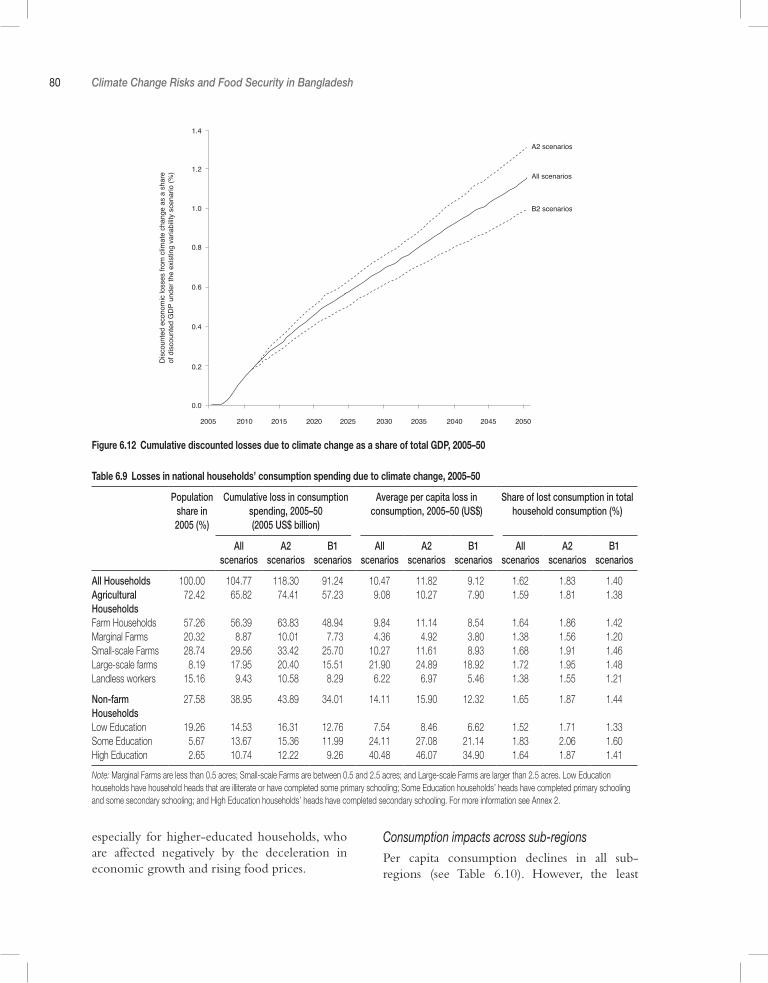
80 Climate Change Risks and Food Security in Bangladesh
Figure 6.12 Cumulative discounted losses due to climate change as a share of total GDP, 2005–50
Table 6.9 Losses in national households’ consumption spending due to climate change, 2005–50
Population share in 2005 (%)
Cumulative loss in consumption spending, 2005–50 (2005 US$ billion)
Average per capita loss in consumption, 2005–50 (US$)
Share of lost consumption in total household consumption (%)
All scenarios
A2 scenarios
B1 scenarios
All scenarios
A2 scenarios
B1 scenarios
All scenarios
A2 scenarios
B1 scenarios
All Households 100.00 104.77 118.30 91.24 10.47 11.82 9.12 1.62 1.83 1.40Agricultural Households
72.42 65.82 74.41 57.23 9.08 10.27 7.90 1.59 1.81 1.38
Farm Households 57.26 56.39 63.83 48.94 9.84 11.14 8.54 1.64 1.86 1.42Marginal Farms 20.32 8.87 10.01 7.73 4.36 4.92 3.80 1.38 1.56 1.20Small-scale Farms 28.74 29.56 33.42 25.70 10.27 11.61 8.93 1.68 1.91 1.46Large-scale farms 8.19 17.95 20.40 15.51 21.90 24.89 18.92 1.72 1.95 1.48Landless workers 15.16 9.43 10.58 8.29 6.22 6.97 5.46 1.38 1.55 1.21
Non-farm Households
27.58 38.95 43.89 34.01 14.11 15.90 12.32 1.65 1.87 1.44
Low Education 19.26 14.53 16.31 12.76 7.54 8.46 6.62 1.52 1.71 1.33Some Education 5.67 13.67 15.36 11.99 24.11 27.08 21.14 1.83 2.06 1.60High Education 2.65 10.74 12.22 9.26 40.48 46.07 34.90 1.64 1.87 1.41
Note: Marginal Farms are less than 0.5 acres; Small-scale Farms are between 0.5 and 2.5 acres; and Large-scale Farms are larger than 2.5 acres. Low Education households have household heads that are illiterate or have completed some primary schooling; Some Education households’ heads have completed primary schooling and some secondary schooling; and High Education households’ heads have completed secondary schooling. For more information see Annex 2.
especially for higher-educated households, who are affected negatively by the deceleration in economic growth and rising food prices.
Consumption impacts across sub-regionsPer capita consumption declines in all sub-regions (see Table 6.10). However, the least
Dis
co
un
ted
eco
no
mic
lo
sse
s f
rom
clim
ate
ch
an
ge
as a
sh
are
of
dis
co
un
ted
GD
P u
nd
er
the
exis
tin
g v
aria
bili
ty s
ce
na
rio
(%
)
0.0
0.2
0.4
0.6
0.8
1.0
1.2
1.4
2005 2010 2015 2020 2025 2030 2035 2040 2045 2050
A2 scenarios
All scenarios
B2 scenarios
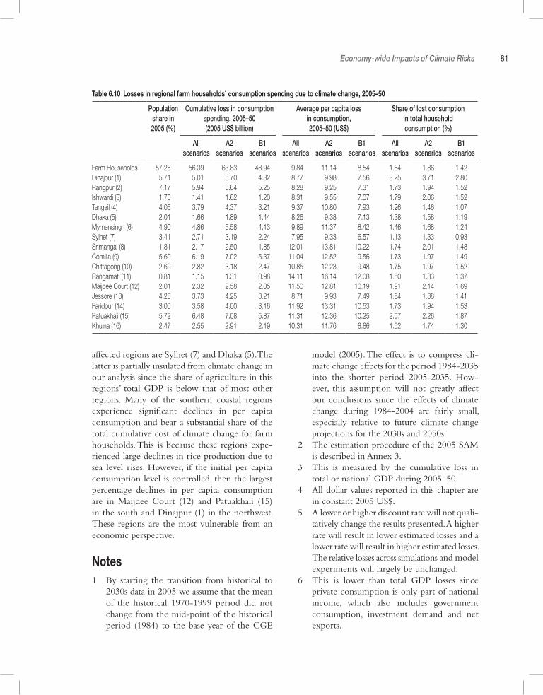
Economy-wide Impacts of Climate Risks 81
affected regions are Sylhet (7) and Dhaka (5). The latter is partially insulated from climate change in our analysis since the share of agriculture in this regions’ total GDP is below that of most other regions. Many of the southern coastal regions experience significant declines in per capita consumption and bear a substantial share of the total cumulative cost of climate change for farm households. This is because these regions expe-rienced large declines in rice production due to sea level rises. However, if the initial per capita consumption level is controlled, then the largest percentage declines in per capita consumption are in Maijdee Court (12) and Patuakhali (15) in the south and Dinajpur (1) in the northwest. These regions are the most vulnerable from an economic perspective.
Notes1 By starting the transition from historical to
2030s data in 2005 we assume that the mean of the historical 1970-1999 period did not change from the mid-point of the historical period (1984) to the base year of the CGE
model (2005). The effect is to compress cli-mate change effects for the period 1984-2035 into the shorter period 2005-2035. How-ever, this assumption will not greatly affect our conclusions since the effects of climate change during 1984-2004 are fairly small, especially relative to future climate change projections for the 2030s and 2050s.
2 The estimation procedure of the 2005 SAM is described in Annex 3.
3 This is measured by the cumulative loss in total or national GDP during 2005–50.
4 All dollar values reported in this chapter are in constant 2005 US$.
5 A lower or higher discount rate will not quali-tatively change the results presented. A higher rate will result in lower estimated losses and a lower rate will result in higher estimated losses. The relative losses across simulations and model experiments will largely be unchanged.
6 This is lower than total GDP losses since private consumption is only part of national income, which also includes government consumption, investment demand and net exports.
Table 6.10 Losses in regional farm households’ consumption spending due to climate change, 2005–50
Population share in 2005 (%)
Cumulative loss in consumption spending, 2005–50 (2005 US$ billion)
Average per capita loss in consumption, 2005–50 (US$)
Share of lost consumption in total household consumption (%)
All scenarios
A2 scenarios
B1 scenarios
All scenarios
A2 scenarios
B1 scenarios
All scenarios
A2 scenarios
B1 scenarios
Farm Households 57.26 56.39 63.83 48.94 9.84 11.14 8.54 1.64 1.86 1.42Dinajpur (1) 5.71 5.01 5.70 4.32 8.77 9.98 7.56 3.25 3.71 2.80Rangpur (2) 7.17 5.94 6.64 5.25 8.28 9.25 7.31 1.73 1.94 1.52Ishwardi (3) 1.70 1.41 1.62 1.20 8.31 9.55 7.07 1.79 2.06 1.52Tangail (4) 4.05 3.79 4.37 3.21 9.37 10.80 7.93 1.26 1.46 1.07Dhaka (5) 2.01 1.66 1.89 1.44 8.26 9.38 7.13 1.38 1.58 1.19Mymensingh (6) 4.90 4.86 5.58 4.13 9.89 11.37 8.42 1.46 1.68 1.24Sylhet (7) 3.41 2.71 3.19 2.24 7.95 9.33 6.57 1.13 1.33 0.93Srimangal (8) 1.81 2.17 2.50 1.85 12.01 13.81 10.22 1.74 2.01 1.48Comilla (9) 5.60 6.19 7.02 5.37 11.04 12.52 9.56 1.73 1.97 1.49Chittagong (10) 2.60 2.82 3.18 2.47 10.85 12.23 9.48 1.75 1.97 1.52Rangamati (11) 0.81 1.15 1.31 0.98 14.11 16.14 12.08 1.60 1.83 1.37Maijdee Court (12) 2.01 2.32 2.58 2.05 11.50 12.81 10.19 1.91 2.14 1.69Jessore (13) 4.28 3.73 4.25 3.21 8.71 9.93 7.49 1.64 1.88 1.41Faridpur (14) 3.00 3.58 4.00 3.16 11.92 13.31 10.53 1.73 1.94 1.53Patuakhali (15) 5.72 6.48 7.08 5.87 11.31 12.36 10.25 2.07 2.26 1.87Khulna (16) 2.47 2.55 2.91 2.19 10.31 11.76 8.86 1.52 1.74 1.30
7
Adaptation Options in the Agriculture Sector
Vulnerability to climate risks and overall eco-nomic development are intricately linked, as is shown in the preceding sections. Therefore, adaptation in the agriculture sector must be well integrated with both the broad national devel-opment goals and livelihood priorities at the local level. Not surprisingly, though, farmers and rural households have long adapted to a variety of climate risks. These coping strategies vary by geographic region and depend on the range of prevailing socio-economic conditions. As the climate changes, more and different adaptations will be required. An approach to studying crop-ping adaptations through the crop simulation approach of Chapter 5 is given in detail in Annex 1. In this chapter, a series of adaptations for which field trials exist and farmer feedback is reported are described. These descriptions provide tem-plates for the development of other adaptations for farm-level implementation.
The presence of both formal and informal sources of support can play a critical role in minimizing climate risks. For instance, substan-tial public-sector investments in agriculture and water have been made to help protect farmers from a variety of existing climate risks. These measures include investments in water infrastruc-ture (e.g. embankments in floodplain and coastal areas to protect against floods and storm surges) and irrigation.
Groundwater irrigation has provided a means for farmers to adapt to soil moisture defi-cits, particularly in drought-prone areas. This has
resulted in changes in cropping pattern, greater diversification of agriculture, promotion of high-yielding varieties and increased cropping inten-sity. Embankments in flood-prone areas (both coastal and inland) have also played a major role in reducing flood risks and protecting key household assets. Over the last three decades, the Bangladesh government has invested over US$10 billion (at constant 2007 prices) for flood management embankments, coastal polder and cyclone shelters (BCAS, personal communica-tion). With this protection, substantial increases in production have been made possible. These collective investments have resulted in significant improvements in meeting national objectives of food-grain self-sufficiency. Substantial invest-ments in early warning and preparedness sys-tems (primarily improvements in flood forecast-ing and cyclone warnings) have also minimized (though not entirely eliminated) the risk from natural disasters. The Bangladesh Disaster Man-agement Bureau plays a critical role in respond-ing to droughts and floods. Lastly, in addition to this direct support from the government depart-ments, non-government organizations and other donors have played an important role in support-ing alternative livelihood activities.
Agriculture research and technology devel-opment has been essential to achieving higher and more stable crop yields. An active network of agriculture research institutes exists in Bang-ladesh. These include the Bangladesh Agricul-ture Research Institute (BARI), Bangladesh
Adaptation Options in the Agriculture Sector 83
Rice Research Institute (BRRI), Bangladesh Institute of Nuclear Agriculture (BINA) and the Bangladesh Agriculture University (BAU). These groups, among other things, develop and test new crop varieties to increase national total production and resilience against climate risks. Extensive testing and field trials are undertaken before new varieties are released to extension organizations for dissemination. The Department of Agriculture Extension (DAE) plays a vital role in disseminating new technologies down to the farmer level through demonstration plots, by providing critical inputs and through training. Typically, DAE undertakes 5–10 demonstrations on a new crop variety at each block each year depending on budget resources. The DAE is one of the largest governmental departments work-ing with approximately 60 per cent of the popu-lation directly involved with crop production. The Department of Agricultural Information Service (AIS) under the DAE is instrumental in preparing materials on specific technology. These institutions will continue to be active in helping Bangladesh achieve food security.
In Bangladesh, though there is no specific drought-tolerant rice variety, DAE does pro-mote particular paddy varieties that are short durational to avoid the effects of drought. These include BR25, BRRI Dhan 33 and BRRI Dhan 39. BARI has also promoted some vegetables and crops like chilli, tomato, okra, cucumber, auber-gine (brinjal/eggplant), potato, cowpea, barley, maize, chickpea, linseed and sesame as drought tolerant. BRRI has developed some flood-toler-ant varieties of paddy including BR11, 20, 21, 22, 23 and 24, and BRRI Dhan 31, 32, 33 and 34. Moreover, as was mentioned earlier, the boro crop plays an important role in offsetting flood losses. Finally, BRRI has developed some saline-resist-ant paddy varieties including BR10 and 23, and BRRI Dhan 32, 41 and 47. Some vegetables and other crops like chilli, tomato, okra, cucumber, potato, cowpea, soybean and barley are promoted as salt tolerant. These evolving new varieties will continue to play a major role in helping farmers adapt to changing and uncertain conditions.
Despite these innovations, poor adoption of technologies and innovations can be common.
The current large gap between actual and poten-tial yields suggests substantial on-farm opportu-nities to increase incomes and production. For many communities, adoption of new technolo-gies can represent high downside risks unless options are well tested in the field. Efforts to provide financial and technical support to ensure sustainable production systems are thus required. Government agriculture extension officers play an important role in these regards. At the house-hold and farm level, private-level adaptations to climate risks have included, inter alia: crop adjust-ments in terms of crop mix and planting dates; supplementary irrigation from ponds; mois-ture conservation approaches; adoption of new seed varieties (e.g. drought and saline resistant), diversifying to fisheries and shrimp production; and flood protection and drainage works. Some current and past adaptation programmes for the agriculture sector in Bangladesh are given in Table 7.1.
7.1 Identifying and Evaluating Adaptation OptionsAdaptation options can address several different types of climate risks. Broadly speaking, adapta-tions can focus on increasing crop productivity, improving irrigation efficiency or expanding water supply, crop diversification and intensifi-cation, generating alternative enterprises (either farm or non-farm sector) to diversify household income sources, and expanding access to train-ing and credit. Existing strategies to deal specifi-cally with drought risks include: full irrigation for dry season boro and supplementary irriga-tion for t. aman from groundwater and surface water sources, crop adjustments (e.g. replanting), moisture conservation practices and promotion of horticultural crops. Existing strategies to deal specifically with flood risks include: construction of embankments and drainage canals, harvesting of crops from under water, changing the crop cal-endar (e.g. late or early planting), raising seedlings in a safe and dry place, double transplanting of seedlings and floating vegetable gardens. Existing strategies to deal with coastal zone risks (e.g. tidal
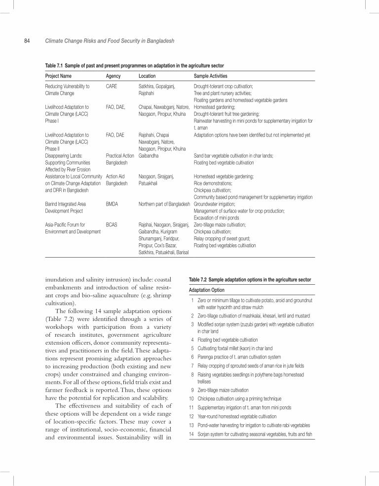
84 Climate Change Risks and Food Security in Bangladesh
inundation and salinity intrusion) include: coastal embankments and introduction of saline resist-ant crops and bio-saline aquaculture (e.g. shrimp cultivation).
The following 14 sample adaptation options (Table 7.2) were identified through a series of workshops with participation from a variety of research institutes, government agriculture extension officers, donor community representa-tives and practitioners in the field. These adapta-tions represent promising adaptation approaches to increasing production (both existing and new crops) under constrained and changing environ-ments. For all of these options, field trials exist and farmer feedback is reported. Thus, these options have the potential for replication and scalability.
The effectiveness and suitability of each of these options will be dependent on a wide range of location-specific factors. These may cover a range of institutional, socio-economic, financial and environmental issues. Sustainability will in
Table 7.1 Sample of past and present programmes on adaptation in the agriculture sector
Project Name Agency Location Sample Activities
Reducing Vulnerability to Climate Change
CARE Satkhira, Gopalganj, Rajshahi
Drought-tolerant crop cultivation; Tree and plant nursery activities; Floating gardens and homestead vegetable gardens
Livelihood Adaptation to Climate Change (LACC) Phase I
FAO, DAE, Chapai, Nawabganj, Natore, Naogaon, Pirojpur, Khulna
Homestead gardening;Drought-tolerant fruit tree gardening;Rainwater harvesting in mini ponds for supplementary irrigation for t. aman
Livelihood Adaptation to Climate Change (LACC) Phase II
FAO, DAE Rajshahi, Chapai Nawabganj, Natore, Naogaon, Pirojpur, Khulna
Adaptation options have been identified but not implemented yet
Disappearing Lands: Supporting Communities Affected by River Erosion
Practical Action Bangladesh
Gaibandha Sand bar vegetable cultivation in char lands;Floating bed vegetable cultivation
Assistance to Local Community on Climate Change Adaptation and DRR in Bangladesh
Action Aid Bangladesh
Naogaon, Sirajganj, Patuakhali
Homestead vegetable gardening;Rice demonstrations;Chickpea cultivation; Community based pond management for supplementary irrigation
Barind Integrated Area Development Project
BMDA Northern part of Bangladesh Groundwater irrigation;Management of surface water for crop production;Excavation of mini ponds
Asia-Pacific Forum for Environment and Development
BCAS Rajshai, Naogaon, Sirajganj, Gaibandha, Kurigram Shunamganj, Faridpur, Pirojpur, Cox’s Bazar, Satkhira, Patuakhali, Barisal
Zero-tillage maize cultivation;Chickpea cultivation;Relay cropping of sweet gourd;Floating bed vegetables cultivation
Table 7.2 Sample adaptation options in the agriculture sector
Adaptation Option
1 Zero or minimum tillage to cultivate potato, aroid and groundnut with water hyacinth and straw mulch
2 Zero-tillage cultivation of mashkalai, khesari, lentil and mustard
3 Modified sorjan system (zuzubi garden) with vegetable cultivation in char land
4 Floating bed vegetable cultivation
5 Cultivating foxtail millet (kaon) in char land
6 Parenga practice of t. aman cultivation system
7 Relay cropping of sprouted seeds of aman rice in jute fields
8 Raising vegetables seedlings in polythene bags homestead trellises
9 Zero-tillage maize cultivation
10 Chickpea cultivation using a priming technique
11 Supplementary irrigation of t. aman from mini ponds
12 Year-round homestead vegetable cultivation
13 Pond-water harvesting for irrigation to cultivate rabi vegetables
14 Sorjan system for cultivating seasonal vegetables, fruits and fish
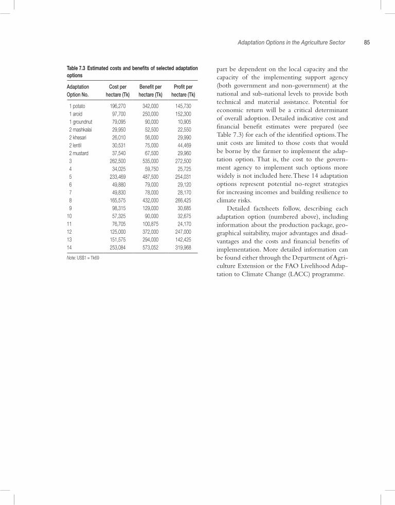
Adaptation Options in the Agriculture Sector 85
part be dependent on the local capacity and the capacity of the implementing support agency (both government and non-government) at the national and sub-national levels to provide both technical and material assistance. Potential for economic return will be a critical determinant of overall adoption. Detailed indicative cost and financial benefit estimates were prepared (see Table 7.3) for each of the identified options. The unit costs are limited to those costs that would be borne by the farmer to implement the adap-tation option. That is, the cost to the govern-ment agency to implement such options more widely is not included here. These 14 adaptation options represent potential no-regret strategies for increasing incomes and building resilience to climate risks.
Detailed factsheets follow, describing each adaptation option (numbered above), including information about the production package, geo-graphical suitability, major advantages and disad-vantages and the costs and financial benefits of implementation. More detailed information can be found either through the Department of Agri-culture Extension or the FAO Livelihood Adap-tation to Climate Change (LACC) programme.
Table 7.3 Estimated costs and benefits of selected adaptation options
Adaptation Option No.
Cost per hectare (Tk)
Benefit per hectare (Tk)
Profit per hectare (Tk)
1 potato 196,270 342,000 145,730 1 aroid 97,700 250,000 152,300 1 groundnut 79,095 90,000 10,905 2 mashkalai 29,950 52,500 22,550 2 khesari 26,010 56,000 29,990 2 lentil 30,531 75,000 44,469 2 mustard 37,540 67,500 29,960 3 262,500 535,000 272,500 4 34,025 59,750 25,725 5 233,469 487,500 254,031 6 49,880 79,000 29,120 7 49,830 78,000 28,170 8 165,575 432,000 266,425 9 98,315 129,000 30,68510 57,325 90,000 32,67511 76,705 100,875 24,17012 125,000 372,000 247,00013 151,575 294,000 142,42514 253,084 573,052 319,968
Note: US$1 = Tk69
86 Climate Change Risks and Food Security in Bangladesh
1 Zero or minimum tillage to cultivate potato, aroid and groundnut with water hyacinth and straw mulch
SummaryThis practice can produce several different types of crops (e.g. potato, aroid, groundnut, chickpea, onion, garlic) with minimum tillage required. This practice is done on mostly medium high land in flood-prone areas during the rabi season. Farmers are already practising this approach when land is unfavourable to normal practices. Farmers sow seeds on moist soil just after the recession of flood water. The land is then mulched with water hyacinth of about 30cm thick. The mulch-ing conserves soil moisture and decreases evapo-ration from the soil. The process is as follows for potato, and similar for the others:
• Clear grasses and debris from the field;• Sowing/planting time is November–Decem-
ber;• Apply fertilizers at the rate of 165kg–100kg–
130kg–40kg/ha of urea-TSP-MOP-gypsum;• Place germinated seed tubers in rows at 60cm
apart and 25cm intervals within a row;• Cover the potato seeds with 30cm thick mass
of water hyacinth;• Depending on the market price the crop can
be harvested partially or fully 70 days after sowing.
Potato is a photo-sensitive, succulent crop that needs more soil moisture during the vegetative period. The water hyacinth is used as a mulch layer to preserve soil moisture as well as increase production. During periods of dense fog and moist weather there is the potential for fungal diseases (like late blight and early blight) that can severely affect potato yield. If this infection hap-pens during the early stages of potato cultivation, production could decrease tremendously.
Most suitable geographic areaCoastal areas (saline and non-saline) and the central floodplains, depending on the degree of
flooding and tidal surge, and areas where mulch materials are readily available are the most suit-able. This is currently practised in Rangpur, Kuri-gram, Gaibandha, Bogra, Sirajgang, Rajshahi, Nawabganj, Natore, Pabna, Kushtia, Faridpur, Munsiganj, Madariganj and Barisal.
Major advantagesThis option provides an additional crop and income for farmers. Farmers can also generate mulch materials as a byproduct of this option which can generate material for household fuel. This byproduct can be sold in the local market. Mulch materials also have the added benefit of protecting soils from high temperatures and high evaporation which increases both microbial activ-ity and soil productivity. Finally, this approach can help to control the population of weeds.
Major disadvantagesThis option will not be feasible without mulch materials such as water hyacinth or straw. Moreo-ver, thin application of mulching materials may not fully protect the tubers from sunlight, result-ing in decreased quality of potato.
Approximate benefitsThis option only requires land, potato seeds, water hyacinth or straw, fungicide and insecti-cides, fertilizers and labour. Approximately a total of Tk196,270 (US$2785) (including land-lease cost) is required to cultivate potato in 1 hectare of land by using this option and farmers can harvest 19.0t of potato at a market price of approximately Tk18 per kg (total Tk342,000 or US$4854). Moreover, farmers can harvest green potatoes as cattle fodder and mulch material as well as fuel for family consumption. Farmers can thus earn a net profit of Tk145,730 (US$2068) from 1 hec-tare of land which would normally remain fallow during the rabi season. Per unit hectare cost of producing aroid and groundnut is Tk97,700 and Tk79,095 (US$1386–1122) respectively. Per hec-tare profits would be approximately Tk152,300 and Tk10,905 (US$2161–154) respectively.
Adaptation Options in the Agriculture Sector 87
2 Zero-tillage cultivation of mashkalai, khesari, lentil and mustard
SummaryIn some cases, after the harvesting of the t. aman crop, the delay in the recession of flood water results in excessive soil moisture and unsuitable conditions for planting. Given this situation, this adaptation option broadcasts mustard, mashkalai or khesari in the t. aman field 10–15 days before harvest using zero tillage approaches to generate an extra crop.
Production packageZero-tillage cultivation of mustard, khesari and mashkalai is currently being practised by farm-ers in flood-prone areas. Farmers sow seeds in the aman paddy fields 10–15 days before harvest time. This is also being grown in previously fal-low fields in mid-October to November after recession of flood waters. The process is as follows for mustard, and similar for the others:
• Method of seed sowing: broadcast;• If possible, supplemental irrigation may pro-
duce better yields (one irrigation during flowering stage and another one during fruit-ing stage);
• For mustard cultivation the following doses of fertilizer might be used for better yield. Urea-TSP-MOP-gypsum-zinc sulphate-boric acid = 225kg–160kg –75kg–140kg–4kg–12kg per hectare;
• Seed rate: Mustard 8–10kg/ha;• Time of harvest: January–February;• Yield: Mustard 1.0–1.5t/ha.
Most suitable geographic areaCoastal areas (saline and non-saline) and central floodplains, depending on the degree of flood-ing and tidal surge, are the most suitable. This is currently practised in Kurigram, Sirajganj, Bogra, Joypurhat, Noagaon, Rajshahi, Jamalpur, Tangail,
Manikganj, Nawabganj, Rajshahi, Pabna, Kushtia, Meherpur, Jessore, Chuadunga, Jhenaida, Farid-pur, Barisal and Narail.
Major advantagesThis option provides an additional crop and income for farmers. Farmers get byproducts that can be used as fodder and for family fuel con-sumption. Pulse crops are also leguminous fam-ily crops which improve soil nutrients through the release of nitrogen. This helps to increase soil productivity. Extension officers, in fact, often advise farmers to harvest the crop from the stem, careful not to uproot the plant. These pulses can add 40–80kg per hectare of nitrogen, i.e. provide about 87–174kg of urea which will decrease fer-tilizer costs.
Major disadvantagesEarly harvest during the vegetative stages may reduce crop yields. During the production period, most of the land remains fallow and may disrupt cattle-grazing practices. Finally, the degree of soil moisture is an important determinant of seed germination. Excess soil moisture could damage seedlings.
Approximate benefitsLand, seeds, fertilizers and labour are required. Approximately a total of Tk37,540 (US$532) is needed to cultivate one hectare of mustard. Farm-ers can harvest 1.5t of mustard at a market price of approximately Tk45 per kg (total Tk67,500 or US$958). Farmers also get the mustard plant as cattle fodder and fuel for family consump-tion. Farmers can earn a net profit of Tk29,960 (US$425) from one hectare of land which nor-mally would have been fallow. The per hectare cost of cultivating khesari, lentil and mashkalai is Tk26,010, Tk30,531 and Tk29,950 (US$369, US$433, US$425) respectively. The net profit is Tk29,990, Tk44,469 and Tk22,550 (US$425, US$631, US$320) for khesari, lentil, and mashka-lai respectively.
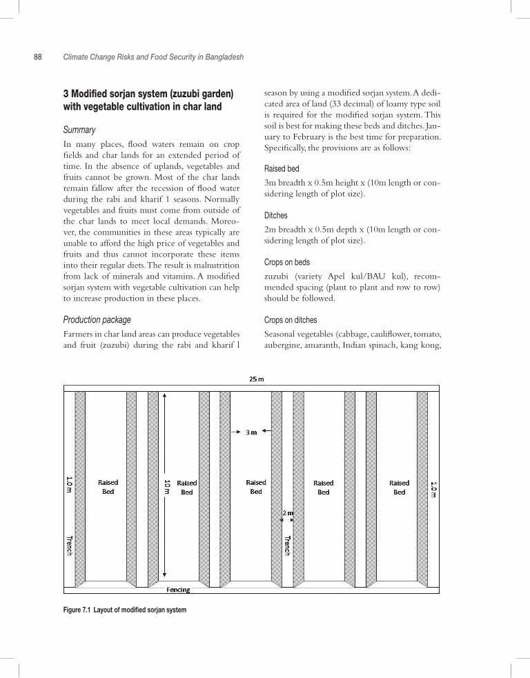
88 Climate Change Risks and Food Security in Bangladesh
3 Modified sorjan system (zuzubi garden) with vegetable cultivation in char land
SummaryIn many places, flood waters remain on crop fields and char lands for an extended period of time. In the absence of uplands, vegetables and fruits cannot be grown. Most of the char lands remain fallow after the recession of flood water during the rabi and kharif 1 seasons. Normally vegetables and fruits must come from outside of the char lands to meet local demands. Moreo-ver, the communities in these areas typically are unable to afford the high price of vegetables and fruits and thus cannot incorporate these items into their regular diets. The result is malnutrition from lack of minerals and vitamins. A modified sorjan system with vegetable cultivation can help to increase production in these places.
Production packageFarmers in char land areas can produce vegetables and fruit (zuzubi) during the rabi and kharif l
season by using a modified sorjan system. A dedi-cated area of land (33 decimal) of loamy type soil is required for the modified sorjan system. This soil is best for making these beds and ditches. Jan-uary to February is the best time for preparation. Specifically, the provisions are as follows:
Raised bed
3m breadth x 0.5m height x (10m length or con-sidering length of plot size).
Ditches
2m breadth x 0.5m depth x (10m length or con-sidering length of plot size).
Crops on beds
zuzubi (variety Apel kul/BAU kul), recom-mended spacing (plant to plant and row to row) should be followed.
Crops on ditches
Seasonal vegetables (cabbage, cauliflower, tomato, aubergine, amaranth, Indian spinach, kang kong,
Figure 7.1 Layout of modified sorjan system
Adaptation Options in the Agriculture Sector 89
chilli, red amaranth, cucumber, bitter gourd, snake gourd , bottle gourd, sweet gourd, etc.) can be cultivated round the year if trellises are made on the ditches.
Fruits
Papaya, lemon, etc. may be planted near the edge of the beds.
Design and layout
• Top soil of middle 2m ditch is removed and kept aside;
• Soil from the 2m plot (ditch) is dug at a depth of 0.5m and placed on the 3m plots;
• The 3m plots are raised to 0.5m high beds to measure three beds at the top;
• The 2m plots at the ends are also dug at a depth of 0.5m and the soil is placed on the beds;
• Slope of the bed is made uniform and com-pact by pressing;
• Top soil kept aside is spread uniformly on the raised bed. Thus the sorjan beds and furrows are made.
• Trellises are made with bamboo and other local materials on the furrows to support creeper vegetables.
Cropping patterns
• The five beds (or more based on the size of the plot) are numbered from 1 to 5 or more. Two beds at either the east or south are ear-marked for vegetables cultivation and the rest for fruits and vegetables.
• The edge of the beds is planted with creeper vegetables, which is supported by the trellis over the furrows.
• Zuzubi should be planted on raised beds fol-lowing standard spacing. Seasonal creeper vegetables can be cultivated on the edges to make trellises on the ditches.
Most suitable geographic areaThe char lands or coastal areas are most suitable depending on the degree of flooding and tidal surges. This is currently being practised in Sirajganj.
Major advantagesThis option helps to diversify the crop mix and increases the production of vegetables and fruits (both for household consumption and for sale in local markets which increases income). This may also have positive nutritional impacts on com-munities in the char lands. The zuzubi plant is a flood-tolerant crop.
Major disadvantagesDepending on the flood frequency and intensity, the ditches may silt with clay and sand. Moreover, large floods may damage the layout of the modi-fied sorjan system. Though the zuzubi plant is a flood-tolerant crop, prolonged exposure to flood waters may still damage the crop and result in disease.
Approximate benefitsThe modified sorjan system requires vegetables seeds, fruits saplings, fertilizers, bamboo, jute sticks, spades and other resources. Approximately a total of Tk233,469 (US$3313) is required to cultivate fruits and vegetables using this approach. A farmer can typically harvest 16,500kg of veg-etables and 3150kg of fruits (zuzubi) where the potential revenue generated is Tk487,500 (US$6920) (assuming Tk20 per kg vegetables and Tk50 per kg of zuzubi). In addition, household consumption of these crops can help to supple-ment family nutritional requirements. Farmers can also use pruned materials for home fuel. In summary, farmers can earn a potential net profit of Tk254,031 (US$3605) from one hectare of char land that would have otherwise remained fallow during the rabi season.
90 Climate Change Risks and Food Security in Bangladesh
4 Floating bed vegetable cultivation
SummaryDuring high floods, land is water-logged and seedlings are easily damaged. In these areas, pro-duction of crops is difficult. Moreover, delayed recession of flood waters can create a scarcity of necessary cereals and vegetables. Considering this, floating vegetable beds (baira) can help to meet the daily requirements for vegetables such as lalshak, data, kang kong, okra, spinach, Indian spinach, cucumber, bitter gourd, bottle gourd, sweet gourd, radish, aubergine, onion and garlic and spices such as chilli and turmeric etc.
Suitable crops for floating bedsAmaranth (both leaf and stem), okra, aubergine, kang kong, etc. can be grown under wet con-ditions on floating substrata made of water hya-cinth. Water hyacinth is abundantly available in flood-prone and submerged areas. This is already being practised in certain locations. Bottle and sweet gourds also can be grown on floating sub-strata, but require that the floating beds touch the ground after the recession of flood water for con-tinued rooting.
Production packages• Make a bamboo frame of 10m long and 1m
wide on water near the land and fix the loca-tion with a bamboo pole;
• Add floating piles of water hyacinth within the bamboo frame and repeat several times at five to seven day intervals on the same piles until a heavy floating bed (about 60cm thick) is made;
• Apply a small dose of TSP and MP on the bed mixed with previously made compost of water hyacinth;
• Mix seeds of red amaranth, stem amaranth, kang kong, okra and a few bottle gourd and sweet gourd seeds in a proportionate quantity, mix with soil and broadcast on the floating bed after five to seven days of application of fertilizers;
• Single crop vegetable seeds with recommended spacing may be sown on the floating bed;
• In a few days the seeds will germinate and grow;
• Apply a little urea depending on the growth of the vegetables;
• Continue to harvest the vegetables by thinning to allow the remaining seedlings to grow.
• When the water recedes the bed will touch the ground and the gourd plants will take root on the field and start fruiting.
• When the bed is about to touch the ground other winter vegetables like cabbage, cauli-flower, etc. can also be planted on the bed ahead of the scheduled planting date and can be grown as a field crop with some fertilizer as needed.
Most suitable geographic areaThe coastal areas (both saline and non-saline areas) and central floodplains are the most suita-ble. The northeast region of the country may also introduce this practice as well. This is currently being practised in Faridpur, Barisal, Gopalganj, Khulna and Gaibandha.
Major advantagesFloating beds (baira) are a low-cost farmer inno-vation that can play a vital role in generating veg-etables for the family. During the dry season, baira can also result in compost to increase soil fertil-ity as well as crop productivity. Farmers can also practise growing tree saplings on baira to generate additional income.
Major disadvantagesHeavy rainfall and strong winds may damage bairas. Sometimes damaged bairas may result in the loss of harvest vegetables. If heavy rains come before germination, seeds may wash away.
Approximate benefitsBamboo for making the baira frame, water hya-cinth, vegetables seeds and some fertilizers are needed for this option. It is estimated that farm-ers can harvest 175kg of vegetables per baira and that about 150 baira can be built on one hec-tare of land. Total harvested vegetables would be approximately 26,250kg. At a market price of

Adaptation Options in the Agriculture Sector 91
about Tk20 (US$0.30) per kg, this results in a total sale value of Tk525,000 (US$7451). Moreo-ver, assuming the generation of 20t of water hya-cinth which can be sold in the market for about Tk10,000 (US$142), the farmer in total will
generate Tk272,500 (US$3867) net on land that otherwise would remain fallow. Furthermore, farmers will consume some vegetables to meet the basic family requirements.

92 Climate Change Risks and Food Security in Bangladesh
5 Cultivating foxtail millet (koan) in char land
SummaryMost of the char lands remain fallow after reces-sion of flood water in rabi and kharif 1 seasons. Foxtail millet (kaon) is a drought-tolerant, short duration crop that can be grown with minimum tillage during the rabi season immediately after the recession of flood water.
Production technologyCurrently, farmers plough their char land two or three times and then sow kaon seeds (10kg per hectare) following a broadcasting or line system. After two to three weeks, seeds germinate and the removal of weeds is needed for better growth and increased yields. Farmers are using urea-TSP-MP fertilizer at the rate of 100kg–75kg–40kg per hectare. If irrigation facilities are available then farmers use half the urea and the total amounts of TSP and MP fertilizer during ploughing of the land; the remainder of the urea may be applied 35–40 days after germination of seed. When irrigation facilities are not available then farm-ers use all the fertilizer during ploughing of the land. Irrigation is needed if drought conditions are prolonged. Normally 2–2.5t of kaon may be produced per hectare of char land.
Most suitable geographic areaThis is most suitable on char lands depending on the occurrence and intensity of the floods. This is
currently being practised in Nilphamari, Rang-pur, Lalmonirhat, Kurigram, Gaibandha, Sirajganj and Jamalpur.
Major advantagesKaon is a low-cost cereal crop that farmers can easily grow on char lands that otherwise would remain fallow during the rabi season. Kaon is also a shallow-rooted crop which can decrease soil erosion and increase organic matter in the soil if, at the time of harvesting, cuttings are made at 20–30cm from the ground.
Major disadvantagesDuring seed germination and seedling stages, prolonged droughts during the rabi season may severely affect the crop. Sometimes, early floods and heavy water-logging may also impact the production.
Approximate benefitsThis is a low-cost activity that needs only mini-mum tillage to prepare the land, kaon seeds and some fertilizer. Farmers can harvest 2.25t of mil-let from one hectare of char land and generate Tk59,750 (US$848) in income. The production cost is Tk34,025 (US$482). Thus, the farmer gets Tk25,725 (US$365) as net profit from one hec-tare of land by using this option. Farmers can also use straw from the millet as fodder for cattle and fuel. This material can be sold in the local market.
Adaptation Options in the Agriculture Sector 93
6 Parenga practice of t. aman cultivation system
SummaryProlonged flooding can damage aman seedlings and also the existing transplanted aman. Moreo-ver, if aman seedlings are damaged, there is often not enough time to re-raise seedlings for trans-planting. Farmers in some places are currently addressing this issue by sowing sprouted aman seeds in moist soil on medium-high or medium-low land after recession of flood waters.
Production packageIn this approach, farmers first clear weeds and other debris from the land. Farmers then soak aman seeds for 24 hours till they sprout and then broadcast (or directly sow) in moist soil during the month of August.
Under this option farmers use urea-TSP-MP-gypsum fertilizers at the rate of 200kg–125kg–85kg–65kg per hectare of land. Farmers apply all of the TSP and gypsum and half of the MP fertilizer after field clearing and then the remainder of the MP and one-third of the urea three to four weeks after sowing. During the till-ing stage, the second dose of urea (one-third of the total dose) may be applied with the remainder of the urea and MP applied immediately before the panicle initiation stage. During the produc-tion period, one to two weedings are needed to decrease infestation of insects and pests. Farmers can harvest 3.5t of paddy from one hectare of land and also get straw that can be used for cattle fodder.
Most suitable geographic areaThis option is most suitable in floodplain areas where flood water recession is late. This option is currently being practised in Kurigram, Gaibandha and Sirajganj.
Major advantagesThis option helps to increase the likelihood of harvesting an additional cereal crop. Farmers also get straw as a byproduct which can be used as fodder for household cattle with the remainder sold in local markets for cash. Finally, because of the increased cropping intensity, the population of weeds is reduced and thus weeding costs for the following crop cycle are reduced.
Major disadvantagesThis option is vulnerable to heavy rainfall and prolonged flooding (especially just after seeds are sown in the field).
Approximate benefitsThe main requirements are medium-to-high land, quality seeds of aman rice, fertilizers, insecticides and pesticides. A total of Tk49,880 (US$708) is needed to cultivate aman rice using the parenga system on one hectare of land. Farmers can har-vest 3.5t of aman rice which at a market value of Tk20 (US$0.30) per kg will gross Tk70,000 (US$993). Furthermore, farmers can get straw for cattle fodder and fuel for family consumption. The remainder can be sold in the local market for cash (approximately Tk9000 or US$128). Farm-ers thus can earn Tk29,120 (US$413) from one hectare of land which would normally remain fallow.
94 Climate Change Risks and Food Security in Bangladesh
7 Relay cropping of sprouted seeds of aman rice in jute fields
SummaryFarmers normally cultivate jute on medium-high land from mid-April to mid-September. Typically after harvest, sowing or transplantation of aman is not possible and so kharif 2 crops are typically not planted and the land remains fallow. To address this, farmers in the southeastern part of Bang-ladesh are practising relay cropping of sprouted aman seeds in jute fields. This approach results in an additional short duration crop on the same field where cultivation of transplanted aman rice would not have been possible.
Production packageFarmers sow jute seeds on medium-high land from mid-April to mid-May and normally har-vest mid-August to mid-September. Sprouted aman seeds are sown on the jute field 15–20 days before harvest/cutting of jute. Farmers select medium-high land where drainage facilities are sufficient and control of water application depth is possible. Before the sowing of aman seeds in the jute fields, the land is cleared of weeds and others debris. Farmers will soak aman seeds for 24 hours for sprouting and then broadcast in the jute field when standing water depth is not more than 2.5–5cm. It is very important to control the water depth of the jute field while the seeds sprout over the next seven days. If water depth cannot be controlled then seeds could be damaged.
Farmers use urea-TSP-MP-gypsum fertiliz-ers at the rate of 200 kg–125kg–85kg–65kg. All the TSP and gypsum and half of the MP fertilizer dose are applied after the jute field is cleared. The remainder of the MP and one-third of the urea is applied three to four weeks after sowing. Dur-ing the tillering stage, the second dose of urea (one-third of total dose) may be applied and the rest of the urea and MP may be applied imme-diately before the panicle initiation stage. During the production period, one to two weedings are required to decrease the susceptibility to insects and pests.
Most suitable geographic area This option is most suitable for medium-high land where sufficient drainage exists. This can also be extended to saline, non-saline and cen-tral floodplain areas where proper infrastructure exists. This option is currently being practised in Faridpur and Barisal.
Major advantagesThis option results in an additional crop which helps to increase total cereal production and gen-erate income for households. Farmers also get straw which can be used as fodder and family fuel consumption.
Major disadvantagesUnder this option it is important to control the water depth during the sowing of seeds in the jute field. If the water depth increases (more than 2.5–5cm of water) and no measures are taken, seeds may get damaged. Also, during the jute cut-ting period, caution must be taken to not damage the aman seedlings. For instance, in some places, the jute plant is left on the fields after cutting which damages the seedlings and reduces overall rice production.
Approximate benefitsResources required include medium-high land, quality seeds of aman rice, fertilizers, insecticides and pesticides. A total of Tk49,830 (US$707) is needed to cultivate aman rice on one hectare of jute field. Farmers can harvest 3.5t of rice which at market price of Tk20 (US$0.30) per kg results in Tk70,000 (US$993) gross. Farmers also get straw byproducts that can be used as cattle fod-der and fuel for family consumption. Remain-der material can be sold in the local market for about Tk8000 (US$113). Farmers thus can earn Tk28,170 (US$400) from one hectare of land that would normally remain fallow after harvest of the jute.
Adaptation Options in the Agriculture Sector 95
8 Raising vegetable seedlings in polythene bags on homestead trellises
SummaryThe floodplain region can sometimes be char-acterized by early floods, prolonged water-log-ging and even late recession of flood water. These problems affect vegetable production during the rabi season. Communities typically need vegeta-ble seedlings for early plantation to harvest before a regular season. Farmers in these areas cannot cultivate winter vegetables due to the unavail-ability of vegetables seedlings. To overcome this, farmers therefore raise vegetable seedlings in pol-ythene bags on trellises near the homestead for early rabi and kharif 1 vegetable production on medium-high land.
Production systemFarmers make covered trellises to overcome the impacts of heavy rainfall and late floods. These are typically located near the homestead. Soil from high lands is mixed with cow dung following the recommended ratio (60:40) and then kept for seven to ten days for decomposition. After that, the mixture is placed in polythene bags (7.5 x 12.5cm) and two to three seeds are sown per poly bag in June to mid-July. These poly bags are then set up on the trellis. Within a few days, seeds are germinated and kept in the trellis for 30–45 days before transplanting on the main land. This coincides with the flood water receding and land thus becomes favourable for ploughing. Farm-ers prepare the field and transplant the seedlings in August to September or as early as possible. Farmers typically cultivate tomato, aubergine, cabbage, etc. using this approach.
Fertilizer doses for some common vegeta-bles:
• Tomato: Urea-TSP-MP and cow dung = 550kg–450kg–250kg–10000kg;
• Aubergine: Urea-TSP-MP and cow dung = 375kg–150kg–250kg–10000kg;
• Cabbage: Urea-TSP-MP and cow dung = 250kg–150kg–200kg–15000 kg.
During land preparation, farmers apply half the cow dung and the total amount of TSP fertiliz-ers. After preparation, beds are raised by about 1m width, 25–30cm height and 25–30cm length depending on land size; 30cm to 35cm of space is kept as a trench between the two beds to use for irrigation water and to drain excess rain-water. Beds are levelled and then seedlings are transplanted during mid-August to September following the spacing for specific vegetables (tomato = 60cm x 40cm; aubergine = 75cm x 60cm; cabbage = 60cm x 45cm). The remain-der of the cow dung is used during plantation of the seedlings and the rest of the fertilizer doses may be applied in the field three to five weeks after plantation. Farmers can harvest on average 36–50t of tomato, aubergine and cabbage on one hectare of land.
In some floodplain regions, farmers are also producing other vegetables (e.g. cucumber, sweet gourd, ash gourd and bitter gourd) in poly bags during the early kharif l season and transplanting on to raised pits of water hyacinth and soil.
Most suitable geographic area The most suitable area for this practice is in flood-prone areas and coastal areas where irriga-tion is available. This is currently being practised in Faridpur, Gopalganj, Barisal and Habiganj.
Major advantagesThis option helps to increase the overall produc-tion of vegetables. This technique helps to over-come the typical water-logging situation which constrains early vegetable production during the rabi season. Farmers also get byproduct materi-als that can be used as cattle fodder. Farmers can sell the vegetable seedlings themselves in the local markets at a high price.
Major disadvantagesSignificant delay in water recession on medium-high land may delay the transplant time which can decrease yields. Long-lasting drought condi-tions during the rabi season might increase irri-gation costs and decrease yields.
96 Climate Change Risks and Food Security in Bangladesh
Approximate benefitsThe resources required include quality vegetable seeds, fertilizers, insecticides, pesticides and suf-ficient medium-high land. A total of Tk165,575 (US$2350) (including land-lease value) is needed to cultivate early rabi vegetables on one hec-tare of land using this option. Farmers on aver-
age can harvest 36–50t of vegetables at a market price of Tk12 (US$0.17) per kg, grossing a total of Tk432,000 (US$6131). Thus, farmers can earn a net profit of Tk266,425 (US$3781) from one hectare of land which normally would not be cul-tivated due to the late recession of flood waters.
Adaptation Options in the Agriculture Sector 97
9 Zero-tillage maize cultivation
SummaryMaize is a crop that grows all year. The yield of maize is comparatively higher than rice, wheat or any other cereal crops. In the Barind tract areas, farmers often harvest and keep t. aman rice on the field to dry for two to three weeks. This is then collected for threshing to separate the rice from the straw. During this time, the soil loses its moisture due to the high rate of evaporation and the land becomes hard. This situation makes it difficult for farmers to plough the land and therefore in many cases the land remains fallow. Farmers can easily cultivate maize by using the existing soil moisture in the fallow land during the rabi season following a zero-tillage system.
Production packageFor cultivating maize using the existing soil moisture on fallow lands, a crop calendar needs to be identified. The exact period of transplan-tation of t. aman seedlings and harvesting dur-ing the kharif 2 season must be determined and coordinated with the maize cultivation. Maize is typically cultivated during the rabi season (seed-sowing time in mid-November to early Decem-ber). Harvested t. aman rice should not be kept on the field. Maize seeds are sown immediately after harvest using a ‘dribbling’ approach whereby a few seeds are sown using a sharp stick or fin-ger. The following steps need to be followed for zero-tillage maize cultivation:
• Weeds and other debris are cleared from the field before sowing seeds;
• Two to five maize seeds are dribbled per hill on no-till muddy soil in 25cm intervals in rows 70cm apart;
• Fertilizers are applied at the following doses: 250kg–200 kg–185 kg–105kg nitrogen- phosphorus-potassium-sulphur (NPKS) per ha land in bands along the maize rows. Fer-tilizers rate for hybrid varieties is 250kg–50kg–140kg–40kg–4kg–2kg/ha of nitrogen-phosphorus-potassium-sulphur-zinc-boron
(NPKSZnB) for high yields and 175kg–40kg–100kg–20kg–2kg–1kg/ha for moder-ate yields;
• Apply all of the PKS and 50 per cent N as the base dose and the remaining N in two equal instalments at 30 and 55 days after sow-ing along the maize rows;
• Keep single maize seeding per hill at 20 days after sowing and use thin plants as fodder;
• Green maize cobs can be harvested depend-ing on need. Mature cobs are harvested at 127 days after sowing;
• Yields of about 4t/ha can be harvested with local composite. Hybrid yields are almost double.
It is to be noted that the land should have the necessary residual moisture to germinate maize seeds. Otherwise, a minimum irrigation may be needed before sowing the maize seeds or after germination. After germination of maize seeds, farmers plough the land by using a spade/hoe and then apply organic and chemical fertilizer mixed with soil. Farmers may irrigate the field accord-ing to the degree of soil moisture and availability of irrigation water to increase the production of maize.
Most suitable geographic areaIn addition to drought-prone areas, the zero-till-age maize cultivation option is also suitable in the coastal saline and non-saline areas and the central floodplains. This is currently being practised in Rajshahi and Nawabganj.
Major advantagesThis option helps to increase the cropping inten-sity and decrease the area of fallow land. This system also helps to increase family income and consumption. Farmers also get byproducts (e.g. stem and cob) which can be sold in the market and/or used to meet family fuel demands. Some farmers also use the stem to make fences to pro-tect homestead-based vegetable gardens. Finally, during the vegetative stage of maize, the leaves can be used as cattle fodder.

98 Climate Change Risks and Food Security in Bangladesh
Major disadvantagesMaize can uptake many nutrients, which decreases overall soil fertility and productivity. Therefore, it should not be used as a mono crop. Presently maize is used only in the poultry sector for poul-try feed.
Approximate benefitsQuality seeds, hoe/spade, labour, fertilizers and pesticides are required. A total of approximately a
Tk98,315 (US$1395) (including land-lease cost) is required to cultivate maize per hectare of land. Farmers can harvest 7.5t of maize. Thus, farmers can earn net Tk30,685 (US$435) from one hec-tare of land that normally would remain fallow during the rabi season.
Adaptation Options in the Agriculture Sector 99
10 Chickpea cultivation using a priming technique
SummaryFarmers typically sow chickpea seeds directly in the field. However, this is not optimal under low soil-moisture conditions. Priming is one approach to address this. In the priming technique, seeds are soaked in water for a period of time based on the thickness of the seed coating. In drier areas, chickpea seeds are soaked at night for a period of six to eight hours. Then the soaked chickpea seeds are spread in a shaded place where there is enough air movement for air drying before sow-ing in the field. After sowing/seeding, the land is ploughed and levelled to preserve the moisture. Good tillage is essential for moisture preserva-tion. Primed seeds will be germinated after four to five days.
Most suitable geographic areaPriming is practised throughout the country depending on the antecedent soil-moisture con-ditions, recession of flood water and seed-sow-ing time. In addition to drought-prone areas, this option is most suitable in the central floodplain, coastal saline and non-saline areas. This is cur-rently being practised in Rajshahi, Nawabganj and Naogaon.
Major advantagesThis option helps to increase pulse production and increase the cropping intensity. In addition to the crop, farmers also get plant and pulse husk byproducts which can be used to meet fodder
and fuel demand and can potentially be used to generate extra income. The chickpea is also a leguminous family plant which absorbs nitrogen and can help increase overall soil productivity. For this reason, the chickpea plant should only be cut after harvest and not entirely uprooted. Moreover, continuous cultivation of chickpeas helps to decrease demand for urea for the next crop. Finally, up to 10–15 crop days are saved by priming.
Major disadvantagesIn the Barind tract areas, farmers are spreading cut t. aman paddy on the fields for prolonged periods thereby increasing the loss of soil mois-ture. This affects the germination of seeds. More-over, in some cases, land cannot be ploughed due to heavy soil and, as a result, most of the land remains fallow.
Approximate benefitsChickpea seeds, fertilizers, bio-fertilizer and insecticides are the major inputs for this practice. Approximately, a total of Tk57,325 (US$813) (included land-lease cost) is needed to cultivate chickpeas on one hectare of land. A farmer can typically harvest 1.8t of chickpeas at a sale value of Tk50 (US$0.70) per kg. Thus, farmers can generate about Tk90,000 (US$1280) in revenues. Farmers also get dry plant and husk byproducts that can be used as cattle fodder and fuel for fam-ily needs. The remainder can be sold in the mar-ket for cash. Farmers, thus, can earn net Tk32,675 (US$463) from one hectare of land during the rabi season.
100 Climate Change Risks and Food Security in Bangladesh
11 Supplementary irrigation of t. aman from mini ponds
SummaryIn the absence of water for irrigation, rainwa-ter harvesting in mini ponds for supplementary irrigation of t. aman during the dry period is an option. These mini ponds are typically excavated within the crop land. Farmers use comparatively lower areas to dig these ponds.
Most suitable geographic areaIn addition to the Barind tract areas, this prac-tice can be implemented in char land and coastal areas depending on the availability of water for irrigation from other sources. This is currently being practised in Rajshahi.
Major advantagesThis option helps to decrease the loss of t. aman production by providing supplemental irrigation. This decreases the dependency on groundwater for irrigation. It is reported that having access to supplemental irrigation can improve rice yields by up to 23 per cent and net economic profit by 75 per cent (FAO LACC Project). Farmers can also cultivate rapid-growth varieties of fish
in these ponds from July to November for both household consumption and market sales. This is an important source of protein for rural com-munities.
Major disadvantagesExcavation of a pond within the crop land reduces the area for crop cultivation. Moreover, due to the soil erosion in the Barind tract, these ponds may become silted in a few years, requir-ing re-excavation.
Approximate benefitsRice seeds, fertilizers, insecticides, pesticides and land are the major inputs to implement this option. Approximately a total of Tk76,705 (US$1088) (included land-lease cost) is needed to cultivate t. aman rice on one hectare of land using this option. Farmers can harvest 4.5t of t. aman and straw (14,500 bundles) for a sale value of Tk90,000 and Tk10,875 (US$1277, US$154) respectively when the unit prices are Tk20 (US$0.30) per kg and Tk0.75 (US$0.01) per bundle. Farmers can also harvest fish. Thus, farmers can earn net Tk24,170 (US$343) from one hectare of land which would normally not be possible.
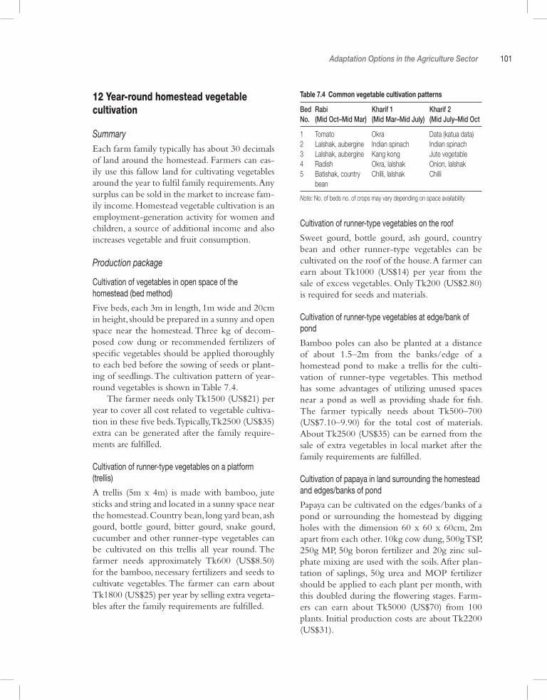
Adaptation Options in the Agriculture Sector 101
12 Year-round homestead vegetable cultivation
SummaryEach farm family typically has about 30 decimals of land around the homestead. Farmers can eas-ily use this fallow land for cultivating vegetables around the year to fulfil family requirements. Any surplus can be sold in the market to increase fam-ily income. Homestead vegetable cultivation is an employment-generation activity for women and children, a source of additional income and also increases vegetable and fruit consumption.
Production package
Cultivation of vegetables in open space of the homestead (bed method)
Five beds, each 3m in length, 1m wide and 20cm in height, should be prepared in a sunny and open space near the homestead. Three kg of decom-posed cow dung or recommended fertilizers of specific vegetables should be applied thoroughly to each bed before the sowing of seeds or plant-ing of seedlings. The cultivation pattern of year-round vegetables is shown in Table 7.4.
The farmer needs only Tk1500 (US$21) per year to cover all cost related to vegetable cultiva-tion in these five beds. Typically, Tk2500 (US$35) extra can be generated after the family require-ments are fulfilled.
Cultivation of runner-type vegetables on a platform (trellis)
A trellis (5m x 4m) is made with bamboo, jute sticks and string and located in a sunny space near the homestead. Country bean, long yard bean, ash gourd, bottle gourd, bitter gourd, snake gourd, cucumber and other runner-type vegetables can be cultivated on this trellis all year round. The farmer needs approximately Tk600 (US$8.50) for the bamboo, necessary fertilizers and seeds to cultivate vegetables. The farmer can earn about Tk1800 (US$25) per year by selling extra vegeta-bles after the family requirements are fulfilled.
Cultivation of runner-type vegetables on the roof
Sweet gourd, bottle gourd, ash gourd, country bean and other runner-type vegetables can be cultivated on the roof of the house. A farmer can earn about Tk1000 (US$14) per year from the sale of excess vegetables. Only Tk200 (US$2.80) is required for seeds and materials.
Cultivation of runner-type vegetables at edge/bank of pond
Bamboo poles can also be planted at a distance of about 1.5–2m from the banks/edge of a homestead pond to make a trellis for the culti-vation of runner-type vegetables. This method has some advantages of utilizing unused spaces near a pond as well as providing shade for fish. The farmer typically needs about Tk500–700 (US$7.10–9.90) for the total cost of materials. About Tk2500 (US$35) can be earned from the sale of extra vegetables in local market after the family requirements are fulfilled.
Cultivation of papaya in land surrounding the homestead and edges/banks of pond
Papaya can be cultivated on the edges/banks of a pond or surrounding the homestead by digging holes with the dimension 60 x 60 x 60cm, 2m apart from each other. 10kg cow dung, 500g TSP, 250g MP, 50g boron fertilizer and 20g zinc sul-phate mixing are used with the soils. After plan-tation of saplings, 50g urea and MOP fertilizer should be applied to each plant per month, with this doubled during the flowering stages. Farm-ers can earn about Tk5000 (US$70) from 100 plants. Initial production costs are about Tk2200 (US$31).
Table 7.4 Common vegetable cultivation patterns
Bed No.
Rabi (Mid Oct–Mid Mar)
Kharif 1 (Mid Mar–Mid July)
Kharif 2 (Mid July–Mid Oct
1 Tomato Okra Data (katua data)2 Lalshak, aubergine Indian spinach Indian spinach3 Lalshak, aubergine Kang kong Jute vegetable4 Radish Okra, lalshak Onion, lalshak5 Batishak, country
beanChilli, lalshak Chilli
Note: No. of beds no. of crops may vary depending on space availability
102 Climate Change Risks and Food Security in Bangladesh
Most suitable geographic areaThis adaptation option is suitable in many dif-ferent areas. In particular, flood-prone, drought-prone, haor (wetland system) and beel (floodplain pond) areas are most suitable. This is currently being practised to varying degrees throughout the country, but limited in scale.
Major advantagesThis option increases family consumption of veg-etables and fruits and improves family income.
Major disadvantagesDue to the intensive use of land for cultivating vegetables and fruits, this option may reduce the overall area devoted to cattle grazing. This
may result in decreases in the availability of cow dung.
Approximate benefitsVegetable seeds, fertilizers, bio-fertilizer, insecti-cides, bamboo, jute sticks and rope are the major materials needed to implement this option. Approximately a total of Tk10,000 (US$142) (considering a 20 decimal homestead area for each family) is needed to cultivate different sea-sonal runner-type vegetables, leafy vegetables and fruits. The farmer will typically get Tk25,000 to Tk35,000 (US$354–496) from the sale of extra vegetables. Farmers may also get plant material that can be used as cattle fodder. Farmers can earn Tk15,000 to Tk20,000 (US$212–283) net from a single farm homestead.
Adaptation Options in the Agriculture Sector 103
13 Pond-water harvesting for irrigation to cultivate rabi vegetables
SummaryFrom October to May, rainfall is very low. The demand for vegetables during the rabi season is high. Winter vegetables require irrigation for maintaining soil moisture at different stages (especially during the vegetative, flowering and fruit-bearing stages). Supplementary irrigation can play a vital role in production of vegetables. In the Barind areas, some farmers are cultivating rabi vegetables with irrigation from mini ponds. Typically, rainwater is harvested or surface water is diverted into mini ponds during the monsoon and then used to grow vegetables during the rabi season. This practice helps to harvest vegetables earlier in the season.
Production packageThe fertilizer dose for tomato is
Urea-TSP-MP and Cow dung = 550kg–450kg–250kg–10,000kg;
for aubergine it is urea-TSP-MP and Cow dung = 375kg–150kg–250kg–10,000kg.
Farmers select land nearest to the pond and pre-pare the land by ploughing and applying half of the cow dung and the total amount of TSP ferti-lizers. After preparation of the land, beds are raised with a width of 1m, a height of 25–30cm and a length depending on land size; 30–40cm of space is kept between beds for irrigation and drain-age of excess rainwater. After levelling the beds, farmers transplant the seedlings, usually from mid-September to November, following the sug-gested spacing for specific vegetables (tomato = 60cm x 40cm; aubergine = 75cm x 60cm). The remainder of the cow dung is used during trans-planting of seedlings. Urea and MP fertilizers are
applied three weeks and five weeks after planting of the vegetable seedlings. Given that these are high value crops, farmers must pay attention to weeding, irrigation, insecticide and pesticide use. About 36–40t of tomato can be harvested from one hectare of land.
Most suitable geographic area The flood-prone and coastal areas are the most suitable. This is currently being practised in Rajshahi, Nawabganj, Naogaon and Natore.
Major advantagesThis option helps to increase vegetable produc-tion and consumption for the family. In drought-prone areas, it is very difficult to cultivate early rabi vegetables without following this option. This reduces the area of fallow land. After the harvest of vegetables, farmers can grow boro rice or high value horticultural crops (e.g. onion, gar-lic). Farmers can also culture fish in these ponds for both household consumption and for sale in local markets.
Major disadvantagesIn the absence of rainfall and the unavailability of surface water, farmers may fail to harvest rain-water in the mini pond. Prolonged droughts may dry out the pond.
Approximate benefitsThe resources required for this option include quality vegetables seeds or seedlings, fertilizers, insecticides, pesticides and land with a mini pond. Tk151,575 (US$2151) is needed to cultivate early vegetables during the rabi season on one hectare of land. A farmer can harvest 24.5t of vegetables which, at a market price of about Tk12 (US$0.17) per kg, will gross Tk294,000 (US$4173). Thus, farmers can earn net Tk142,425 (US$2021) from one hectare of land.
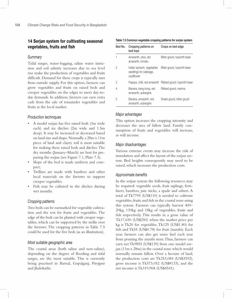
104 Climate Change Risks and Food Security in Bangladesh
14 Sorjan system for cultivating seasonal vegetables, fruits and fish
SummaryTidal surges, water-logging, saline water intru-sion and soil salinity increases due to sea level rise make the production of vegetables and fruits difficult. Demand for these crops is typically met from outside supply. For this option, farmers can grow vegetables and fruits on raised beds and creeper vegetables on the edges to meet day-to-day demands. In addition, farmers can earn extra cash from the sale of remainder vegetables and fruits at the local market.
Production techniques• A model sorjan has five raised beds (3m wide
each) and six ditches (2m wide and 1.5m deep). It may be increased or decreased based on land size and shape. Normally a 28m x 11m piece of land and clayey soil is most suitable for making these raised beds and ditches. The dry months (January–March) are best for pre-paring the sorjan (see Figure 7.1, Plate 7.3).
• Slope of the bed is made uniform and com-pact;
• Trellises are made with bamboo and other local materials on the furrows to support creeper vegetables.
• Fish may be cultured in the ditches during wet months.
Cropping patternsTwo beds can be earmarked for vegetable cultiva-tion and the rest for fruits and vegetables. The edge of the beds can be planted with creeper vege-tables, which can be supported by the trellis over the furrows. The cropping patterns in Table 7.5 could be used for the five beds (as an illustration).
Most suitable geographic area The coastal areas (both saline and non-saline), depending on the degree of flooding and tidal surges, are the most suitable. This is currently being practised in Barisal, Gopalganj, Pirojpur and Jhalokathi.
Major advantagesThis option increases the cropping intensity and decreases the area of fallow land. Family con-sumption of fruits and vegetables will increase, as will income.
Major disadvantagesVarious extreme events may increase the risk of inundation and affect the layout of the sorjan sys-tem. Bed heights consequently may need to be raised, which increases the production costs.
Approximate benefitsIn the sorjan system the following resources may be required: vegetable seeds, fruit saplings, ferti-lizers, bamboo, jute sticks, a spade and others. A total of Tk7795 (US$110) is needed to cultivate vegetables, fruits and fish in the coastal zone using this system. Farmers can typically harvest 400–20kg, 130kg and 18kg of vegetables, fruits and fish respectively. This results in a gross value of Tk17,650 (US$250) when the market price per kg is Tk20 for vegetables, Tk125 (US$1.80) for fish and Tk55 (US$0.78) for fruit (zuzubi). Each year, farmers can also get some fuel each year from pruning the zuzubi stem. Thus, farmers can earn net Tk9855 (US$139) from one model sor-jan (11m x 28m) in the coastal zone which would normally remain fallow. Over a hectare of land, the production costs are Tk253,084 (US$3592), gross income is Tk573,052 (US$8133), and the net income is Tk319,968 (US$4541).
Table 7.5 Common vegetable cropping patterns for sorjan system
Bed No. Cropping patterns on bed tops
Crops on bed edge
1 Amaranth, okra, red amaranth, tomato
Bitter gourd, hyacinth bean
2 Indian spinach, vegetables seedlings for cabbage, cauliflower
Bitter gourd, hyacinth bean
3 Papaya, chilli, red amaranth Ribbed gourd, hyacinth bean
4 Banana, kang kong, red amaranth, aubergine
Ribbed gourd, marma
5 Banana, amaranth, red amaranth, aubergine
Snake gourd, bitter gourd
8
The Way Forward – Turning Ideas into Action
The year 2007 was indicative of the challenges that Bangladesh faces to achieving food security. Severe flooding from July to September 2007 affected over 13 million people in 46 districts and caused extensive damage to agricultural pro-duction and physical assets (e.g. housing, embank-ments). With hardly any time to recover, on 15 November 2007 Cyclone Sidr made landfall across the southern coast of the country, causing over 3000 deaths. The total economic damages of these two events amounted to over US$1 billion US (World Bank, 2008). Moreover almost 2 mil-lion tonnes of rice were lost, putting government cereal stocks in a precarious situation. Finally, that same year the unabated increase in the interna-tional prices of oil and food, of which Bangladesh is a net importer, put further strains on both gov-ernment budgets and household livelihoods.
What these events demonstrated was the inherent vulnerability of Bangladesh to climate risks. It also showed the degree to which food security remains a challenge for the country. Cli-mate change has the potential to significantly affect Bangladesh’s efforts to provide food to a growing nation. The challenges that the agricul-ture sector will face as it adapts to climate change, however, coincide well with the needs required to address the climate variability risks of today. Both processes of adapting to climate change and stimulating the agriculture sector to achieve rural growth and support livelihoods require efforts to, among other things: diversify household income sources; improve crop productivity; support greater
agricultural research and development; promote education and skills development; increase access to financial services; enhance irrigation efficiency and overall water and land productivity; strengthen climate risk management; and develop protective infrastructure. Continued developmental plan-ning and investment is needed to build resilience at both national and local scales.
This study is largely focused on the impacts of climate risks (both climate variability and climate change) on food security in Bangladesh. The risks from climate change include higher temperatures and changing precipitation patterns, increased flood intensity and frequency, droughts and sea level rise effects on agriculture production. The future is also expected to bring elevated CO
2 con-
centrations, which have a beneficial effect on crop growth. A suite of models is used to approach the complex questions of climate variability and change and food security in Bangladesh. In this study, future climate is projected using the most recent climate science available. Detailed hydro-logic models project changes in future flooding. Country specific data is used to derive more realistic and accurate agricultural impact func-tions and simulations. Finally, a dynamic CGE is used to better understand the degree to which economic effects will buffer against the physical losses predicted from climate variability and cli-mate change. Significant impacts on growth and household consumption are projected.
The models used here are among the best mathematical representations available of the
106 Climate Change Risks and Food Security in Bangladesh
physical and economic responses to these exog-enous climate changes. However, like all modell-ing approaches, uncertainty exists as parameters may not be known with precision and functional forms may not be fully accurate. Thus, careful sensitivity analysis and an understanding and appreciation of the limitations of these models are required. Further collection and analysis of critical input and output observations (e.g. cli-mate data, farm-level practices and irrigation constraints) will enhance this integrated frame-work methodology and future climate impact assessments.
Some key messages that emerge from this study include:
The impacts of existing climate variability are enormous. A no-regret strategy is to focus first on the near-term climate risks to build future resilience
Bangladesh is clearly one of the most vulnerable countries to climate risks today. The agriculture sector is impacted by annual flooding, water shortages during the dry season and frequent coastal cyclones and storm surges. Though the relative severity of these disasters has decreased substantially since the 1970s, these remain criti-cal challenges to rural poverty and growth. Thus, continued substantial public investment in protective infrastructure (e.g. cyclone shelters, embankments), early warning and preparedness systems and programmes to build resilience at the household level (e.g. income diversification, identified adaptation options in this study) can play a critical role in minimizing these impacts.
The impacts of future changes in temperatures and precipitation, increased CO
2 levels, flooding,
droughts and sea level rise are highly uncertain. In some cases not only is the magnitude of change not known with precision, but also the direction of change. Despite this, the simulation estimates in this study suggest that the simulated cumula-tive economy-wide impacts of existing climate variability alone (US$594 billion) are almost five times that of climate change (US$129 bil-lion). That is, the existing inter- and intra-annual variation is significantly larger than the projected
uncertain future changes. This, however, is not a cause for inaction. Rather, a no-regrets strategy is to promote activities and policies that help the national government and households build resil-ience in the agriculture sector to existing climate risks today. This aligns well with existing devel-opment strategies and plans. By doing so, the country and households will be better prepared for whichever future outcome materializes. The adaptation options identified are only a small sub-set of what can be done today.
The southern and northwestern regions are the most vulnerable. This is due to the confluence of several different climate risks and existing poor baseline conditions
From a socio-economic perspective, the south and northwest regions have long been areas of extensive poverty. As these communities cur-rently in many cases exist on the margins, both climate variability and climate change threaten to increase these vulnerabilities. The sub-regions in the south sit at the confluence of multiple climate risks. These areas experience the largest decline in rice production due to climate change. This is for three reasons. First, these regions already experience significant declines in aus and aman rice production due to climate variability, which is expected to worsen under climate change. Second, boro yields are severely affected by the effects of changes in mean rainfall and tempera-ture. Thus, reductions in boro production limit the ability for these regions to compensate for lost aus and aman rice production during extreme events. Projections, moreover, are conservative as access to irrigation is assumed limitless. Third, the south is also affected the most by rising sea lev-els, which permanently reduces cultivable land. The largest percentage declines in per capita consumption will be in these regions. Similarly, the northwest region is particularly vulnerable as impacts have a disproportionate share relative to the low existing household consumption. These two areas are where priority must be given and where substantial opportunities for adaptation are possible.
The Way Forward – Turning Ideas to Action 107
Increased investments in adaptation in the agriculture sector are critical to ensuring continued growth and poverty alleviation
Bangladesh will continue to depend on the agriculture sector for economic growth. Rural households will continue to depend on the agri-culture sector for income and livelihoods. Floods, droughts and cyclones will continue to affect the performance of the agriculture sector. Though the government has made substantial investments to increase the resilience of the poor (e.g. new high-yielding crop varieties, protective infrastructure, disaster management), as has been shown these variability impacts may be exacerbated by long-term effects of climate change.
Households have for a long time adapted to these dynamic conditions to maintain their liveli-hoods. The nature of these adaptations and the determinants of success depend on the availabil-ity of assets, resources, labour, skills, education and social capital. The adaptation options iden-tified, in fact, are currently being implemented in many locations with assistance from both the government and donor community. However, the scale of these efforts remains limited and is not commensurate with the probable impacts. Moreover, the current large gap between actual and potential yields suggests substantial on-farm opportunities for growth and poverty reduction. Expanded availability of modern rice varieties, irrigation facilities, fertilizer use and labour could increase average yields at rates that could poten-tially more than offset the climate change impacts. Significant additional planning and investments in promoting these types of adaptations are still needed.
8.1 A Framework for Assessing the Economic Impacts of Climate ChangeThe precise impact of climate change on coun-tries in the developing world remains to be seen. This much is known, however: climate change poses additional risks to many developing coun-tries in their efforts to reduce poverty, promote
livelihoods and develop sustainably. As popula-tions grow, the ability for many countries to meet basic food requirements and effectively manage future disasters will be critical for sus-taining long-term economic growth. These are challenges above and beyond those that many countries are already currently facing. Moreover, most developing countries lack the financial and technical capacities to manage these increasing risks. Thus, strategic prioritization and improved planning and management of existing assets and budget resources are critical. Largely, these strate-gic choices will be dependent on the economics of these impacts.
The integrated framework used in this analy-sis provides a broad and unique approach to esti-mating the hydrologic and biophysical impacts of climate change, the macro-economic and household-level impacts and an effective method for assessing a variety of adaptation practices and policies. The framework presented here can serve as a useful guide to other countries and regions faced with similar development chal-lenges and objectives of achieving food security. In assessing the impacts, several different mod-elling environments must be integrated to pro-vide a more nuanced and complete picture of how food security may be impacted by climate change. This approach is needed to better under-stand the relative impacts from multiple climate risks (e.g. floods, droughts, climate change) and how these relate in the context of an evolving socio-economic baseline (e.g. population, prices, international trade). Moreover, such a framework allows for extensive scenario analysis to identify and understand key sensitivities. This is critical to making decisions in a highly uncertain future. Finally, through this integration of multiple disci-plines, a richer and more robust set of adaptation options and policies for the agriculture sector can be identified and tested. Continued refine-ments to the assessment approach developed in this volume will further help to sharpen criti-cal policies and interventions by the Bangladesh government.
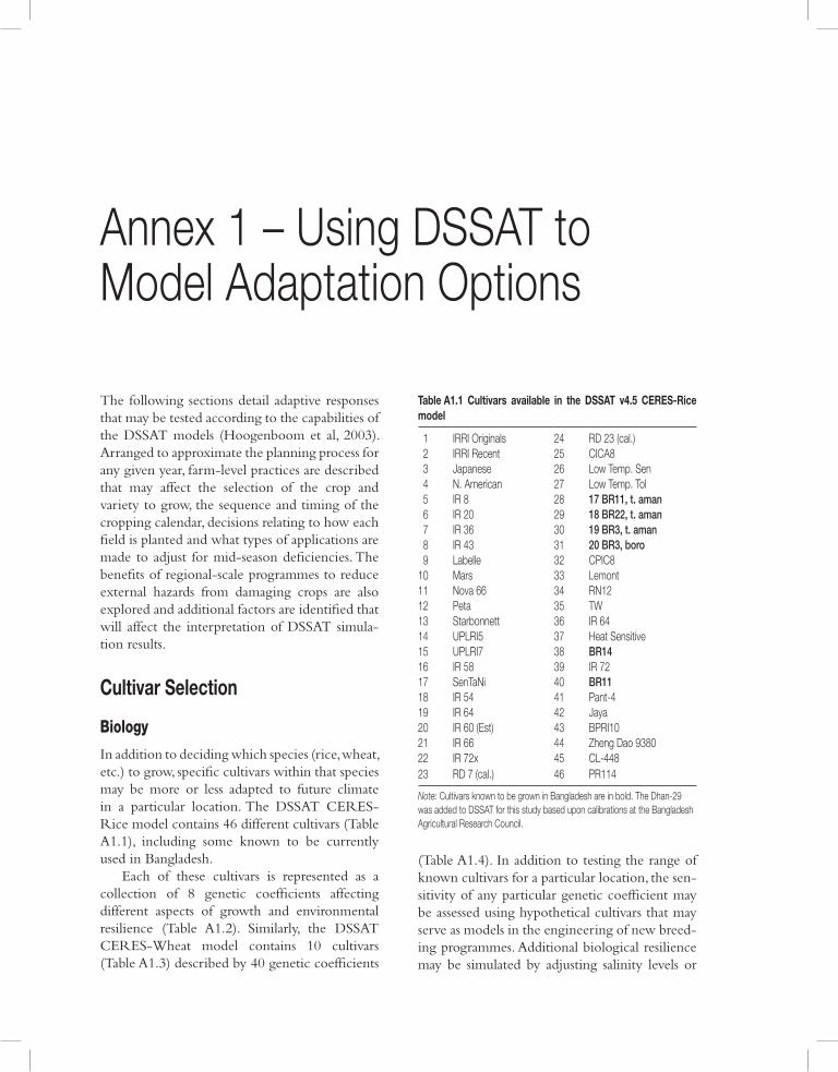
Annex 1 – Using DSSAT to Model Adaptation Options
The following sections detail adaptive responses that may be tested according to the capabilities of the DSSAT models (Hoogenboom et al, 2003). Arranged to approximate the planning process for any given year, farm-level practices are described that may affect the selection of the crop and variety to grow, the sequence and timing of the cropping calendar, decisions relating to how each field is planted and what types of applications are made to adjust for mid-season deficiencies. The benefits of regional-scale programmes to reduce external hazards from damaging crops are also explored and additional factors are identified that will affect the interpretation of DSSAT simula-tion results.
Cultivar Selection
Biology
In addition to deciding which species (rice, wheat, etc.) to grow, specific cultivars within that species may be more or less adapted to future climate in a particular location. The DSSAT CERES-Rice model contains 46 different cultivars (Table A1.1), including some known to be currently used in Bangladesh.
Each of these cultivars is represented as a collection of 8 genetic coefficients affecting different aspects of growth and environmental resilience (Table A1.2). Similarly, the DSSAT CERES-Wheat model contains 10 cultivars (Table A1.3) described by 40 genetic coefficients
(Table A1.4). In addition to testing the range of known cultivars for a particular location, the sen-sitivity of any particular genetic coefficient may be assessed using hypothetical cultivars that may serve as models in the engineering of new breed-ing programmes. Additional biological resilience may be simulated by adjusting salinity levels or
Table A1.1 Cultivars available in the DSSAT v4.5 CERES-Rice model
1 IRRI Originals 24 RD 23 (cal.) 2 IRRI Recent 25 CICA8 3 Japanese 26 Low Temp. Sen 4 N. American 27 Low Temp. Tol 5 IR 8 28 17 BR11, t. aman 6 IR 20 29 18 BR22, t. aman 7 IR 36 30 19 BR3, t. aman 8 IR 43 31 20 BR3, boro 9 Labelle 32 CPIC810 Mars 33 Lemont11 Nova 66 34 RN1212 Peta 35 TW13 Starbonnett 36 IR 6414 UPLRI5 37 Heat Sensitive15 UPLRI7 38 BR1416 IR 58 39 IR 7217 SenTaNi 40 BR1118 IR 54 41 Pant-419 IR 64 42 Jaya20 IR 60 (Est) 43 BPRI1021 IR 66 44 Zheng Dao 938022 IR 72x 45 CL-44823 RD 7 (cal.) 46 PR114
Note: Cultivars known to be grown in Bangladesh are in bold. The Dhan-29 was added to DSSAT for this study based upon calibrations at the Bangladesh Agricultural Research Council.
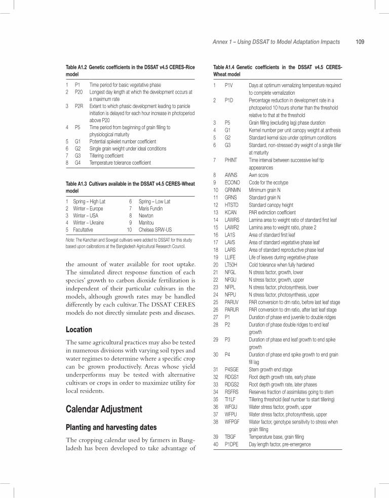
Annex 1 – Using DSSAT to Model Adaptation Impacts 109
the amount of water available for root uptake. The simulated direct response function of each species’ growth to carbon dioxide fertilization is independent of their particular cultivars in the models, although growth rates may be handled differently by each cultivar. The DSSAT CERES models do not directly simulate pests and diseases.
Location
The same agricultural practices may also be tested in numerous divisions with varying soil types and water regimes to determine where a specific crop can be grown productively. Areas whose yield underperforms may be tested with alternative cultivars or crops in order to maximize utility for local residents.
Calendar Adjustment
Planting and harvesting dates
The cropping calendar used by farmers in Bang-ladesh has been developed to take advantage of
Table A1.2 Genetic coefficients in the DSSAT v4.5 CERES-Rice model
1 P1 Time period for basic vegetative phase2 P20 Longest day length at which the development occurs at
a maximum rate3 P2R Extent to which phasic development leading to panicle
initiation is delayed for each hour increase in photoperiod above P20
4 P5 Time period from beginning of grain filling to physiological maturity
5 G1 Potential spikelet number coefficient6 G2 Single grain weight under ideal conditions7 G3 Tillering coefficient8 G4 Temperature tolerance coefficient
Table A1.3 Cultivars available in the DSSAT v4.5 CERES-Wheat model
1 Spring – High Lat 6 Spring – Low Lat2 Winter – Europe 7 Maris Fundin3 Winter – USA 8 Newton4 Winter – Ukraine 9 Manitou5 Facultative 10 Chelsea SRW-US
Note: The Kanchan and Sowgat cultivars were added to DSSAT for this study based upon calibrations at the Bangladesh Agricultural Research Council.
Table A1.4 Genetic coefficients in the DSSAT v4.5 CERES-Wheat model
1 P1V Days at optimum vernalizing temperature required to complete vernalization
2 P1D Percentage reduction in development rate in a photoperiod 10 hours shorter than the threshold relative to that at the threshold
3 P5 Grain filling (excluding lag) phase duration 4 G1 Kernel number per unit canopy weight at anthesis5 G2 Standard kernel size under optimum conditions6 G3 Standard, non-stressed dry weight of a single tiller
at maturity7 PHINT Time interval between successive leaf tip
appearances8 AWNS Awn score9 ECONO Code for the ecotype10 GRNMN Minimum grain N 11 GRNS Standard grain N 12 HTSTD Standard canopy height13 KCAN PAR extinction coefficient14 LAWRS Lamina area to weight ratio of standard first leaf15 LAWR2 Lamina area to weight ratio, phase 216 LA1S Area of standard first leaf17 LAVS Area of standard vegetative phase leaf18 LARS Area of standard reproductive phase leaf19 LLIFE Life of leaves during vegetative phase20 LT50H Cold tolerance when fully hardened21 NFGL N stress factor, growth, lower22 NFGU N stress factor, growth, upper23 NFPL N stress factor, photosynthesis, lower24 NFPU N stress factor, photosynthesis, upper25 PARUV PAR conversion to dm ratio, before last leaf stage26 PARUR PAR conversion to dm ratio, after last leaf stage27 P1 Duration of phase end juvenile to double ridges28 P2 Duration of phase double ridges to end leaf
growth29 P3 Duration of phase end leaf growth to end spike
growth30 P4 Duration of phase end spike growth to end grain
fill lag31 P4SGE Stem growth end stage32 RDGS1 Root depth growth rate, early phase33 RDGS2 Root depth growth rate, later phases34 RSFRS Reserves fraction of assimilates going to stem35 TI1LF Tillering threshold (leaf number to start tillering)36 WFGU Water stress factor, growth, upper37 WFPU Water stress factor, photosynthesis, upper38 WFPGF Water factor, genotype sensitivity to stress when
grain filling39 TBGF Temperature base, grain filling40 P1DPE Day length factor, pre-emergence
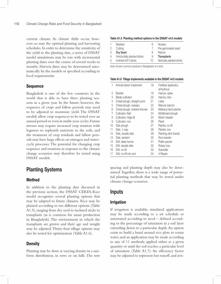
110 Climate Change Risks and Food Security in Bangladesh
current climate. As climate shifts occur, how-ever, so may the optimal planting and harvesting schedules. In order to determine the sensitivity of the yield to the planting date, a series of DSSAT model simulations may be run with incremental planting dates over the course of several weeks to months. Harvest dates may be determined auto-matically by the models or specified according to local requirements.
Sequence
Bangladesh is one of the few countries in the world that is able to have three planting sea-sons in a given year. In the future, however, the sequence of crops and fallow periods may need to be adjusted to maximize yield. The DSSAT models allow crop sequences to be tested over an annual period or even in multi-year cycles. Future stresses may require increased crop rotation with legumes to replenish nutrients in the soils, and the treatment of crop residuals and fallow peri-ods may have large effects on nitrogen and water-cycle processes. The potential for changing crop sequence and rotations in response to the climate change scenarios may therefore be tested using DSSAT models.
Planting Systems
Method
In addition to the planting date discussed in the previous section, the DSSAT CERES-Rice model recognizes several planting options that may be adapted to future climates. Rice may be planted according to ten different options (Table A1.5), ranging from dry seed to inclined sticks to transplants (as is common for aman production in Bangladesh). The environment in which the transplants are grown and their age and weight may be adjusted. Thirty-four tillage options may also be tested for optimization (Table A1.6).
Density
Planting may be done at varying density in a uni-form distribution, in rows or on hills. The row
spacing and planting depth may also be deter-mined. Together, there is a wide range of poten-tial planting methods that may be tested under climate change scenarios.
Inputs
Irrigation
If irrigation is available, simulated applications may be made according to a set schedule or automated according to need – defined accord-ing to the percentage of saturation in a soil layer extending down to a particular depth. An option exists to build a bund around rice plots to retain water, and an application may be made according to any of 11 methods; applied either as a given quantity or until the soil reaches a particular level of saturation (Table A1.7). An efficiency factor may be adjusted to represent lost runoff, and irri-
Table A1.5 Planting method options in the DSSAT v4.5 models
1 Bedded 6 Nursery2 Cutting 7 Pre-germinated seed3 Dry Seed 8 Ratoon4 Horizontally planted sticks 9 Transplants5 Inclined (45°) sticks 10 Vertically planted sticks
Note: Known common practices in Bangladesh is in bold.
Table A1.6 Tillage implements available in the DSSAT v4.5 models
1 Animal-drawn implement 18 Fertilizer applicator, anhydrous
2 Bedder 19 Harrow, spike 3 Blade cultivator 20 Harrow, tine 4 Chisel plough, straight point 21 Lister 5 Chisel plough, sweeps 22 Manure injector 6 Chisel plough, twisted shovels 23 Matraca hand planter 7 Cultivator, field 24 Moldboard plough 8 Cultivator, ridge till 25 Mulch treader 9 Cultivator, row 26 Plank10 Disk plough 27 Planter, no-till11 Disk, 1-way 28 Planter, row12 Disk, double disk 29 Planting stick (hand)13 Disk, tandem 30 Rod weeder14 Drill, deep furrow 31 Roller packer15 Drill, double-disk 32 Rotary hoe16 Drill, no-till 33 Subsoiler17 Drill, no-till into sod 34 V-Ripper
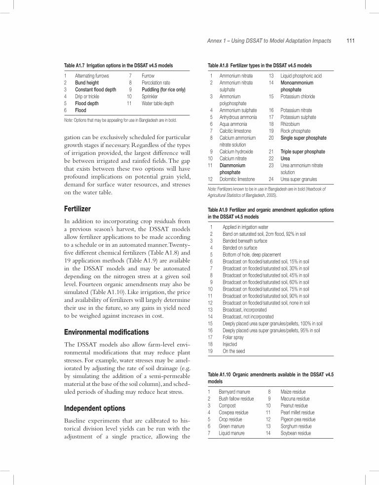
Annex 1 – Using DSSAT to Model Adaptation Impacts 111
gation can be exclusively scheduled for particular growth stages if necessary. Regardless of the types of irrigation provided, the largest difference will be between irrigated and rainfed fields. The gap that exists between these two options will have profound implications on potential grain yield, demand for surface water resources, and stresses on the water table.
Fertilizer
In addition to incorporating crop residuals from a previous season’s harvest, the DSSAT models allow fertilizer applications to be made according to a schedule or in an automated manner. Twenty-five different chemical fertilizers (Table A1.8) and 19 application methods (Table A1.9) are available in the DSSAT models and may be automated depending on the nitrogen stress at a given soil level. Fourteen organic amendments may also be simulated (Table A1.10). Like irrigation, the price and availability of fertilizers will largely determine their use in the future, so any gains in yield need to be weighed against increases in cost.
Environmental modifications
The DSSAT models also allow farm-level envi-ronmental modifications that may reduce plant stresses. For example, water stresses may be amel-iorated by adjusting the rate of soil drainage (e.g. by simulating the addition of a semi-permeable material at the base of the soil column), and sched-uled periods of shading may reduce heat stress.
Independent options
Baseline experiments that are calibrated to his-torical division level yields can be run with the adjustment of a single practice, allowing the
Table A1.7 Irrigation options in the DSSAT v4.5 models
1 Alternating furrows 7 Furrow2 Bund height 8 Percolation rate3 Constant flood depth 9 Puddling (for rice only)4 Drip or trickle 10 Sprinkler5 Flood depth 11 Water table depth6 Flood
Note: Options that may be appealing for use in Bangladesh are in bold.
Table A1.8 Fertilizer types in the DSSAT v4.5 models
1 Ammonium nitrate 13 Liquid phosphoric acid 2 Ammonium nitrate
sulphate14 Monoammonium
phosphate 3 Ammonium
polyphosphate15 Potassium chloride
4 Ammonium sulphate 16 Potassium nitrate 5 Anhydrous ammonia 17 Potassium sulphate 6 Aqua ammonia 18 Rhizobium 7 Calcitic limestone 19 Rock phosphate 8 Calcium ammonium
nitrate solution20 Single super phosphate
9 Calcium hydroxide 21 Triple super phosphate10 Calcium nitrate 22 Urea11 Diammonium
phosphate23 Urea ammonium nitrate
solution12 Dolomitic limestone 24 Urea super granules
Note: Fertilizers known to be in use in Bangladesh are in bold (Yearbook of Agricultural Statistics of Bangladesh, 2005).
Table A1.9 Fertilizer and organic amendment application options in the DSSAT v4.5 models
1 Applied in irrigation water 2 Band on saturated soil, 2cm flood, 92% in soil 3 Banded beneath surface 4 Banded on surface 5 Bottom of hole, deep placement 6 Broadcast on flooded/saturated soil, 15% in soil 7 Broadcast on flooded/saturated soil, 30% in soil 8 Broadcast on flooded/saturated soil, 45% in soil 9 Broadcast on flooded/saturated soil, 60% in soil10 Broadcast on flooded/saturated soil, 75% in soil11 Broadcast on flooded/saturated soil, 90% in soil12 Broadcast on flooded/saturated soil, none in soil13 Broadcast, incorporated14 Broadcast, not incorporated15 Deeply placed urea super granules/pellets, 100% in soil16 Deeply placed urea super granules/pellets, 95% in soil17 Foliar spray18 Injected19 On the seed
Table A1.10 Organic amendments available in the DSSAT v4.5 models
1 Barnyard manure 8 Maize residue2 Bush fallow residue 9 Macuna residue3 Compost 10 Peanut residue4 Cowpea residue 11 Pearl millet residue5 Crop residue 12 Pigeon pea residue6 Green manure 13 Sorghum residue7 Liquid manure 14 Soybean residue
112 Climate Change Risks and Food Security in Bangladesh
sensitivity of yield to each particular approach to be evaluated. Yield sensitivity for each of the following management practices (as applicable) may then be assessed for any given location and climate scenario:
• Crop selection• Known cultivar selection• Genetic coefficient values• Soil profile• Tillage schedule• Tillage implement• Tillage depth• Planting date• Planting density• Planting geometry• Planting depth• Planting method• Temperature of transplant environment (if
applicable)• Transplant age (if applicable)• Transplant weight (if applicable)• Irrigation calendar• Irrigation type• Irrigation amount• Fertilizer calendar• Fertilizer type• Fertilizer implementation option• Organic amendment calendar• Organic amendment type• Organic amendment implementation option• Harvest date• Environmental modifications• External flood control• External salinity control.
Combined practices
Once sensitive practices are identified, strategies may be developed to combine adapted practices for maximum seasonal yield. If multiple strate-gies produce similar shifts in yield, the cost-
effectiveness of each approach may be evalu-ated along with the extent to which the new management departs from traditional practices. Assumptions about water management may also be incorporated to determine irrigation avail-ability and develop strategies to maintain scarce resources. This allows a projected benefit to be associated with the cost of each simulated adapta-tion option. Some potential combined practices include modifications to:
• Cultivar selection and irrigation calendar• Planting density and planting depth• Tillage implement and fertilizer implementa-
tion option• Cultivar selection, irrigation amount and ferti-
lizer type• Cultivar selection, planting date, and irriga-
tion amount• Genetic coefficient values, planting date, plant-
ing method, planting geometry, planting depth, irrigation calendar, irrigation amount, irrigation type, fertilizer calendar, fertilizer type, fertilizer amount and fertilizer imple-mentation option.
Sequential adjustments
The DSSAT crop modelling system allows for simulations of crop cycling that allows evalua-tion of multi-seasonal adaptation strategies. The inclusion of a legume cycle or a multi-seasonal strategy of fertilizer application may be a cost-effective way to maximize yield from a particular plot of land. The effect of changing one season’s practices may be assessed for lingering impacts on the following seasons using this crop model-ling framework. Thus, the cropping strategy of a particular location may be analysed throughout an annual or multi-year cycle of cultivation and fallow periods to maximize sustainability and yields.
Annex 2 – Description of the CGE Model
Tables A2.1 and A2.2 present the equations of a simple closed-economy computable general equilibrium (CGE) model that is used at this stage to illustrate how climate change affects the economic outcomes examined in this analysis. The model is recursive dynamic and can there-fore be separated into a static ‘within-period’ component wherein producers and consum-ers maximize profits and utility, and a dynamic ‘between-period’ component wherein the model is updated based on the demographic model and previous period results, thereby reflecting changes in population, labour supply, and the accumula-tion of capital and technology.
In the static component of the model, pro-ducers in each sector s and agro-climatic region r produce a level of output Q in time period t by employing the factors of production F under constant returns to scale (exogenous productivity α) and fixed production technologies (fixed fac-tor shares δ) – Equation 1. Profit maximization implies that factor payments W are equal to aver-age production revenues – Equation 2. Labour supply L, land supply N and capital supply K are fixed within a given time period, implying full employment of factor resources. Land and labour market equilibrium is defined at the regional level, so land and labour is mobile across sec-tors but wages and rental rates vary by region – Equation 6. National capital market equilib-rium implies that capital is mobile across both sectors and regions, and earns a national rental rate (i.e. regional capital returns are equalized) – Equation 8.
Factor incomes are distributed to households in each region using fixed income shares based on the households’ initial factor endowments – Equation 3. Total household incomes Y are then either saved (based on marginal propensities to save υ) or spent on consumption C (accord-ing to marginal budget shares β) – Equation 4. Consumption spending includes a ‘subsistence’ component λ that is independent of income and determined by household population H. Savings are collected in a national savings pool and used to finance investment demand I (i.e., savings-driven investment closure) – Equation 5. Finally, a single price P equilibrates national product markets, thus avoiding the necessity of modelling inter-regional trade flows – Equation 9.
The model variables and parameters are cali-brated to observed data from a regional social accounting matrix (SAM) (described in Annex 3) that captures the initial equilibrium structure of the economy in 2005. Parameters are then adjusted over time to reflect demographic and economic changes and the model is resolved for a series of new equilibriums for the 45-year period 2005–50. Three dynamic adjustments occur between periods: changes in land and labour sup-ply; capital accumulation; and technical change.
Between periods the model is updated to reflect long-term growth rates in land supply N and labour supply L. These are imposed through the parameters σ and φ – Equations 10 and 11 – which remain unchanged across simulations. For capital supply K, the model endogenously determines the national rate of accumulation – Equation 12.
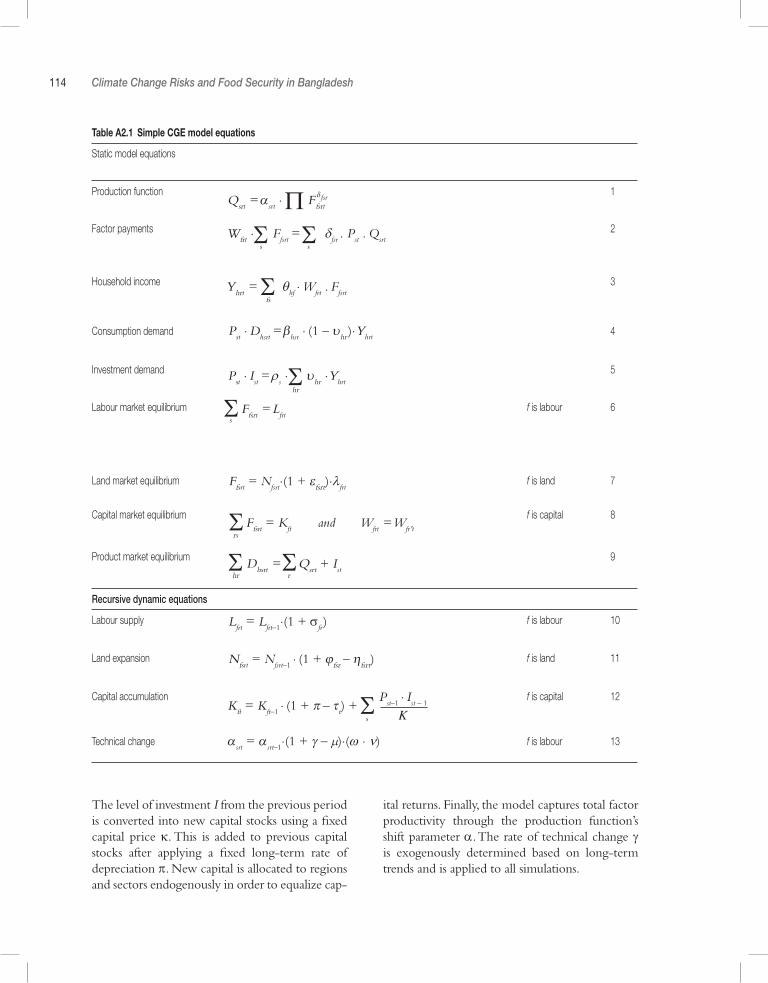
114 Climate Change Risks and Food Security in Bangladesh
Table A2.1 Simple CGE model equations
Static model equations
Production function 1
Factor payments 2
Household income 3
Consumption demand 4
Investment demand 5
Labour market equilibrium f is labour 6
Land market equilibrium f is land 7
Capital market equilibrium f is capital 8
Product market equilibrium 9
Recursive dynamic equations
Labour supply f is labour 10
Land expansion f is land 11
Capital accumulation f is capital 12
Technical change f is labour 13
The level of investment I from the previous period is converted into new capital stocks using a fixed capital price κ. This is added to previous capital stocks after applying a fixed long-term rate of depreciation π. New capital is allocated to regions and sectors endogenously in order to equalize cap-
ital returns. Finally, the model captures total factor productivity through the production function’s shift parameter α. The rate of technical change γ is exogenously determined based on long-term trends and is applied to all simulations.
αsrt = α
srt–1.(1 + γ – µ).(ω . ν)
Lfrt = L
frt–1.(1 + σ
fr )
Ffsrt = Nfsrt
.(1 + εfsrt).λfrt
Pst . Dhsrt =
β
hsr . (1 – υhr ).Yhrt
Nfsrt = Nfsrt–1
. (1 + ϕfsr – ηfsrt)
Kft = Kft–1
. (1 + π – τt) +
Qsrt = α
srt .Π F δfsrt
fsr
Wfrt . Ffsrt
=
δfsr
. Pst . Q
srtΣ Σs s
Yhrt = θ
hf . W
frt . F
fsrtΣfs
Pst . Ist =
ρ
s . υhr .YhrtΣ
hr
Ffsrt = L
frtΣs
Dhsrt = Qsrt + I
stΣhr
Σr
Ffsrt = Kft and W
frt = W
fr 'tΣrs
Σs
Pst–1
. Ist – 1
K
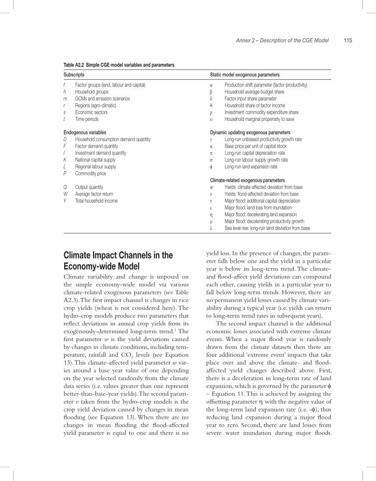
Annex 2 – Description of the CGE Model 115
Climate Impact Channels in the Economy-wide ModelClimate variability and change is imposed on the simple economy-wide model via various climate-related exogenous parameters (see Table A2.3). The first impact channel is changes in rice crop yields (wheat is not considered here). The hydro-crop models produce two parameters that reflect deviations in annual crop yields from its exogenously-determined long-term trend.1 The first parameter w is the yield deviations caused by changes in climate conditions, including tem-perature, rainfall and CO
2 levels (see Equation
13). This climate-affected yield parameter w var-ies around a base year value of one depending on the year selected randomly from the climate data series (i.e. values greater than one represent better-than-base-year yields). The second param-eter v taken from the hydro-crop models is the crop yield deviation caused by changes in mean flooding (see Equation 13). When there are no changes in mean flooding the flood-affected yield parameter is equal to one and there is no
yield loss. In the presence of changes, the param-eter falls below one and the yield in a particular year is below its long-term trend. The climate- and flood-affect yield deviations can compound each other, causing yields in a particular year to fall below long-term trends. However, there are no permanent yield losses caused by climate vari-ability during a typical year (i.e. yields can return to long-term trend rates in subsequent years).
The second impact channel is the additional economic losses associated with extreme climate events. When a major flood year is randomly drawn from the climate datasets then there are four additional ‘extreme event’ impacts that take place over and above the climate- and flood-affected yield changes described above. First, there is a deceleration in long-term rate of land expansion, which is governed by the parameter φ – Equation 11. This is achieved by assigning the offsetting parameter η with the negative value of the long-term land expansion rate (i.e. -φ), thus reducing land expansion during a major flood year to zero. Second, there are land losses from severe water inundation during major floods.
Table A2.2 Simple CGE model variables and parameters
Subscripts Static model exogenous parameters
f Factor groups (land, labour and capital) α Production shift parameter (factor productivity)h Household groups β Household average budget sharem GCMs and emission scenarios δ Factor input share parameterr Regions (agro-climatic) θ Household share of factor incomes Economic sectors ρ Investment commodity expenditure sharet Time periods υ Household marginal propensity to save
Endogenous variables Dynamic updating exogenous parametersD Household consumption demand quantity γ Long-run unbiased productivity growth rateF Factor demand quantity κ Base price per unit of capital stockI Investment demand quantity π Long-run capital depreciation rateK National capital supply σ Long-run labour supply growth rateL Regional labour supply φ Long-run land expansion rateP Commodity price
Climate-related exogenous parametersQ Output quantity w Yields: climate-affected deviation from baseW Average factor return v Yields: flood-affected deviation from baseY Total household income τ Major flood: additional capital depreciation
ε Major flood: land loss from inundationη Major flood: decelerating land expansion µ Major flood: decelerating productivity growth λ Sea level rise: long-run land deviation from base
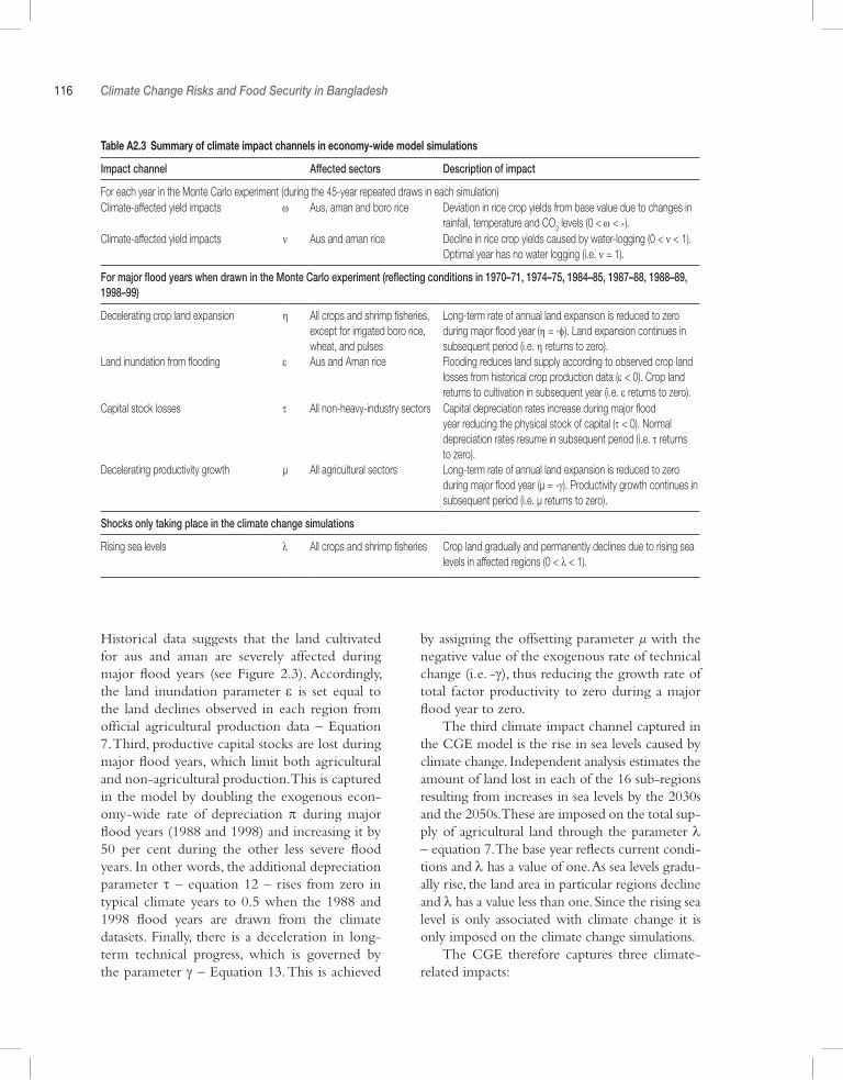
116 Climate Change Risks and Food Security in Bangladesh
Table A2.3 Summary of climate impact channels in economy-wide model simulations
Impact channel Affected sectors Description of impact
For each year in the Monte Carlo experiment (during the 45-year repeated draws in each simulation)Climate-affected yield impacts ω Aus, aman and boro rice Deviation in rice crop yields from base value due to changes in
rainfall, temperature and CO2 levels (0 < ω < ∞).Climate-affected yield impacts ν Aus and aman rice Decline in rice crop yields caused by water-logging (0 < ν < 1).
Optimal year has no water logging (i.e. ν = 1).
For major flood years when drawn in the Monte Carlo experiment (reflecting conditions in 1970–71, 1974–75, 1984–85, 1987–88, 1988–89, 1998–99)
Decelerating crop land expansion η All crops and shrimp fisheries, except for irrigated boro rice, wheat, and pulses
Long-term rate of annual land expansion is reduced to zero during major flood year (η = -φ). Land expansion continues in subsequent period (i.e. η returns to zero).
Land inundation from flooding ε Aus and Aman rice Flooding reduces land supply according to observed crop land losses from historical crop production data (ε < 0). Crop land returns to cultivation in subsequent year (i.e. ε returns to zero).
Capital stock losses τ All non-heavy-industry sectors Capital depreciation rates increase during major flood year reducing the physical stock of capital (τ < 0). Normal depreciation rates resume in subsequent period (i.e. τ returns to zero).
Decelerating productivity growth µ All agricultural sectors Long-term rate of annual land expansion is reduced to zero during major flood year (µ = -γ). Productivity growth continues in subsequent period (i.e. µ returns to zero).
Shocks only taking place in the climate change simulations
Rising sea levels λ All crops and shrimp fisheries Crop land gradually and permanently declines due to rising sea levels in affected regions (0 < λ < 1).
Historical data suggests that the land cultivated for aus and aman are severely affected during major flood years (see Figure 2.3). Accordingly, the land inundation parameter ε is set equal to the land declines observed in each region from official agricultural production data – Equation 7. Third, productive capital stocks are lost during major flood years, which limit both agricultural and non-agricultural production. This is captured in the model by doubling the exogenous econ-omy-wide rate of depreciation π during major flood years (1988 and 1998) and increasing it by 50 per cent during the other less severe flood years. In other words, the additional depreciation parameter τ – equation 12 – rises from zero in typical climate years to 0.5 when the 1988 and 1998 flood years are drawn from the climate datasets. Finally, there is a deceleration in long-term technical progress, which is governed by the parameter γ – Equation 13. This is achieved
by assigning the offsetting parameter µ with the negative value of the exogenous rate of technical change (i.e. -γ), thus reducing the growth rate of total factor productivity to zero during a major flood year to zero.
The third climate impact channel captured in the CGE model is the rise in sea levels caused by climate change. Independent analysis estimates the amount of land lost in each of the 16 sub-regions resulting from increases in sea levels by the 2030s and the 2050s. These are imposed on the total sup-ply of agricultural land through the parameter λ – equation 7. The base year reflects current condi-tions and λ has a value of one. As sea levels gradu-ally rise, the land area in particular regions decline and λ has a value less than one. Since the rising sea level is only associated with climate change it is only imposed on the climate change simulations.
The CGE therefore captures three climate-related impacts:
Annex 2 – Description of the CGE Model 117
1 Yield losses each year resulting from potential sub-optimal climate conditions (including temperature, rainfall, CO
2 and mean flood
changes) as estimated by the hydro-crop models;
2 Lost land, capital and productivity growth during major flood years as observed in his-torical production data;
3 Lost cultivable land resulting from rising sea levels caused by climate change.
The economy-wide model also accounts for the predicted increase in the frequency of major flooding resulting from climate change. The return period for the 1988 and 1998 flood years are reduced by one-third. In other words, 1988 and 1998 are characterized as the 1/33 and 1/50 year floods respectively (in relation to water dis-charges). The frequency of these floods in the sample for the random selection of years for the future climate sequences is increased to 1/25 and 1/33 for the 1988 and 1998 floods respectively.
Extensions in the Full Bangladesh ModelThe simplified model illustrates how climate var-iability and change affects economic outcomes in our analysis. However, the full Bangladesh model drops certain assumptions.2 Constant elasticity of substitution (CES) production functions allows factor substitution based on relative factor prices (i.e. δ is no longer fixed). The model identifies 36 sectors in each of the 16 agro-climatic regions (i.e. 17 in agriculture, 14 in industry and 5 in services). Intermediate demand in each sector (excluded from the simple model) is determined by fixed technology coefficients. Based on the 2005 household income and expenditure survey, labour markets are further segmented across four skill groups:
1 Illiterate or uneducated workers; 2 Workers with primary education;3 Workers with some secondary schooling; 4 Workers with secondary or higher schooling.
Farm land is divided into:
1 Marginal farms with less than 0.5 acres; 2 Small-scale farms with between 0.5 and 2.5
acres; 3 Large-scale farms with more than 2.5 acres.
All factors are assumed to be fully employed, and capital is immobile across sectors. New capital from past investment is allocated to regions/sec-tors according to profit rate differentials under a ‘putty-clay’ specification.
The full model still assumes national product markets. However, international trade is captured by allowing production and consumption to shift imperfectly between domestic and foreign mar-kets, depending on the relative prices of imports, exports and domestic goods. Since Bangladesh is a relatively small economy, world prices are assumed to be fixed and the current account bal-ance is maintained by a flexible real exchange rate (i.e. the price index of tradable-to-non-trad-able goods). Production and trade elasticities are econometrically estimated.
A linear expenditure system determines household consumption levels and permits non-unitary income elasticities. Households are disag-gregated across agricultural and nonagricultural groups. Agricultural households are separated into landowners and landless agricultural work-ers. Landowning farm households in each of the 16 agro-climatic regions are separated into mar-ginal, small-scale and large-scale farm households. Non-agricultural households are disaggregated according to the education level of their house-hold head (i.e. uneducated or illiterate, primary-school educated and secondary-school edu-cated or higher). There are a total of 52 distinct household groups in the full CGE model. These household groups pay taxes to the government based on fixed direct and indirect tax rates. Tax revenues finance exogenous recurrent spending, resulting in an endogenous fiscal deficit.
Notes1 The base year crop yields in the CGE model
(i.e. 2005) are set as the average yield achieved

118 Climate Change Risks and Food Security in Bangladesh
for a given agro-climatic region and crop dur-ing the 1970–99 baseline. These then grow at an exogenous rate reflecting the long-term rate of technical change without the effects of climate variability or change.
2 A mathematical specification of the under-lying recursive dynamic CGE model is pre-
sented in Thurlow (2004). The CGE model used in the current study falls within the broader class of structural neo-classical models described in Dervis et al (1982) and Robinson (1989).
Annex 3 – Constructing the Social Accounting Matrix for Bangladesh
Key Features of the 2005 Bangladesh SAMA social accounting matrix (SAM) is a consist-ent data framework that captures the information contained in the national income and product accounts and the input-output table, as well as the monetary flows between institutions. A SAM is an ex-post accounting framework because, within its square matrix, total receipts must equal total payments for each account contained within the SAM. Since the required data is not drawn from a single source, information from various sources must be compiled and made consistent. This process is valuable since it identifies incon-sistencies among Bangladesh’s statistical sources and highlights areas where data reliability is weak-est. SAMs are economy-wide databases which are used in conjunction with analytical techniques to strengthen the evidence underlying policy deci-sions. The 2005 SAM extends previous SAMs constructed by the International Food Policy Research Institute (IFPRI) by including more agricultural sectors, and disaggregating agri-cultural production across 64 districts/zilas and non-agricultural production across the 6 major regional divisions/states of the country.
General structure of SAMs
A SAM is an economy-wide data framework that usually represents the real economy of a single country.1 More technically, a SAM is a square matrix in which each account is represented by a row and column. Each cell shows the payment from the account of its column to the account of its row – the incomes of an account appear along its row, its expenditures along its column. The underlying principle of double-entry accounting requires that, for each account in the SAM, total revenue (row total) equals total expenditure (col-umn total). Table A3.1 shows an aggregate SAM (with verbal explanations in place of numbers).
The SAM distinguishes between ‘activi-ties’ (the entities that carry out production) and ‘commodities’ (representing markets for goods and non-factor services). SAM flows are valued at producers’ prices in the activity accounts and at market prices (including indirect commodity taxes and transactions costs) in the commodity accounts. The commodities are activity outputs, either exported or sold domestically, and imports. In the activity columns, payments are made to commodities (intermediate demand) and factors of production (value-added comprising operat-ing surplus and compensation of employees). In the commodity columns, payments are made to domestic activities, the rest of the world and

Tabl
e A3
.1 B
asic
stru
ctur
e of
a S
AM
Activ
ities
Com
mod
ities
Fact
ors
Hous
ehold
sGo
vern
men
tInv
estm
ent
Rest
of th
e W
orld
Tota
l
Activ
ities
Mar
kete
d ou
tput
Activ
ity in
com
e
Com
mod
ities
Inter
med
iate
input
sPr
ivate
con
sum
ption
Gove
rnm
ent
cons
umpt
ionInv
estm
ent,
chan
ge
in sto
cks
Expo
rtsTo
tal d
eman
d
Fact
ors
Value
-add
edFa
ctor
inco
me
Hous
ehold
sFa
ctor
inco
me
to
hous
ehold
sTra
nsfer
s to
hous
ehold
sFo
reign
rem
ittanc
es
rece
ived
Hous
ehold
inco
me
Gove
rnm
ent
Sales
taxe
s, im
port
tariff
sFa
ctor
and
cor
pora
te
taxe
sDi
rect
hou
seho
ld ta
xes
Gove
rnm
ent t
rans
fers
from
rest
of w
orld
Gove
rnm
ent in
com
e
Savin
gsHo
useh
old sa
vings
Gove
rnm
ent s
aving
sFo
reign
savin
gsSa
vings
Rest
of th
e W
orld
Impo
rtsRe
patri
ated
ear
nings
Gove
rnm
ent t
rans
fers
to re
st of
wor
ldFo
reign
exc
hang
e ou
tflow
Tota
lAc
tivity
exp
endit
ures
Tota
lsu
pply
Fact
or e
xpen
ditur
esHo
useh
old
expe
nditu
res
Gove
rnm
ent
expe
nditu
res
Inves
tmen
tFo
reign
exc
hang
e infl
ow
Annex 3 – Constructing the Social Accounting Matrix for Bangladesh 121
various tax accounts (for domestic and import taxes). This treatment provides the data needed to model imports as perfect or imperfect substitutes vis-à-vis domestic production.
The government is disaggregated into a core government account and different tax collection accounts, one for each tax type. This disaggrega-tion is necessary since otherwise the economic interpretation of some payments is often ambig-uous. In the SAM, direct payments between the government and households are reserved for transfers. Finally, payments from the government to factors (for the labour services provided by public-sector employees) are captured in the gov-ernment services activity. Government consump-tion demand is a purchase of the output from the government services activity, which in turn pays labour.
The SAM contains a number of factors of production, which earn incomes from their use in the production process and then pay their incomes to households, government and the rest of the world. Capital earnings or profits are taxed according to average corporate tax rates and some profits may be repatriated abroad. The remaining capital earnings, together with other factors’ earnings (e.g. land and labour) are paid to households. Households use their incomes to pay taxes, save, and consume domestically produced and imported commodities.
Structure of the 2005 Bangladesh SAM
The new SAM extends previous Bangladesh SAMs produced by IFPRI by: (1) updating the previous 2002/03 SAM to 2004/05; (2) disag-gregating the agricultural sector across a greater number of crops; (3) disaggregating agricul-tural production and land and livestock markets across 64 districts or zilas; and (4), disaggregat-ing non-agricultural production and labour and capital markets across 6 divisions. The next sec-tion describes the various data sources used to produce the new 2005 SAM, while this section describes its overall structure.
The SAM identifies 62 sectors, of which 23 are in agriculture (see Table A3.2). Agricultural production is divided into crop agriculture (18
sub-sectors), livestock (2 sub-sectors), fisheries (2 sub-sectors) and forestry. With the exception of forestry and ‘other fisheries’, which are disaggre-gated across divisions, all agricultural sub-sectors are disaggregated across Bangladesh’s 64 districts or zilas. Given severe land constraints in Bang-ladesh, agricultural land is disaggregated across three categories: (1) marginal farmers (farm households with less than 0.5 acres of cultivated land); (2) small-scale farmers (households with between 0.5 and 2.5 acres of cultivated land); and (3) medium- and large-scale farmers (house-hold with more than 2.5 acres of cultivated land – equivalent to 1 hectare of land). Land alloca-tion across crops varies across different parts of the country and across farm households with dif-ferent land endowments (see Table A3.3). Farm households’ land endowments are typically small in Bangladesh, with the average farm household cultivating just over 1 acre of land. This varies sig-nificantly across divisions, with the largest average cultivated land sizes in Rajshahi and the smallest in Chittagong and Dhaka. This aggregation hides even greater variation across districts. All farm households devote a majority of their land to rice production, although most households produce a diverse range of crops. This regional and sectoral heterogeneity justifies the detailed spatial disag-gregation of crops in the new Bangladesh SAM.
The 2005 SAM retains non-agriculture sec-toral detail from the 2002/03 IFPRI SAM, but these non-agricultural sectors are now disaggre-gated across six regional divisions (see Table A3.4). The Dhaka division is the largest in terms of its contribution to gross domestic product (GDP), accounting for two-fifths of the overall economy. Agriculture is least important in the Dhaka divi-sion, accounting for 10 per cent of its economy, which is substantially below the national aver-age contribution of agriculture of 20 per cent of GDP. Agriculture is especially important for the smaller divisions of Barisal, Khulna and Sylhet, where the sector accounts for around a third to a half of divisional GDP.
Factors markets are defined at various levels of spatial aggregation. Land and livestock capital are specific to each zila and, as mentioned above, agricultural land in each zila is further disag-
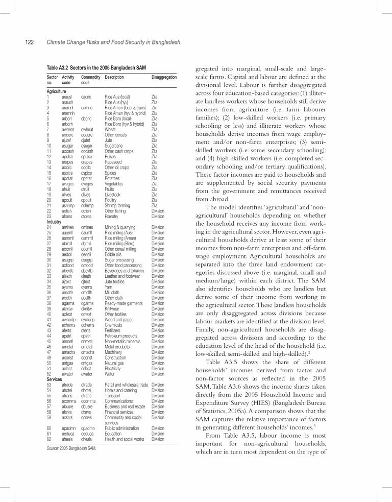
122 Climate Change Risks and Food Security in Bangladesh
Table A3.2 Sectors in the 2005 Bangladesh SAM
Sector no.
Activity code
Commodity code
Description Disaggregation
Agriculture1 arausl cauric Rice Aus (local) Zila2 araush Rice Aus (hyv) Zila3 aramnl camric Rice Aman (local & trans) Zila4 aramnh Rice Aman (hyv & hybrid) Zila5 arborl cboric Rice Boro (local) Zila6 arborh Rice Boro (hyv & hybrid) Zila7 awheat cwheat Wheat Zila8 aocere cocere Other cereals Zila9 ajutef cjutef Jute Zila10 asugar csugar Sugarcane Zila11 aocash cocash Other cash crops Zila12 apulse cpulse Pulses Zila13 arapes crapes Rapeseed Zila14 aooilc cooilc Other oil crops Zila15 aspice cspice Spices Zila16 apotat cpotat Potatoes Zila17 aveges cveges Vegetables Zila18 afruit cfruit Fruits Zila19 alives clives Livestock Zila20 apoult cpoult Poultry Zila21 ashrmp cshrmp Shrimp farming Zila22 aofish cofish Other fishing Division23 afores cfores Forestry DivisionIndustry24 amines cmines Mining & quarrying Division25 aaumll caumll Rice milling (Aus) Division26 aammll cammll Rice milling (Aman) Division27 abrmll cbrmll Rice milling (Boro) Division28 aocmll cocmll Other cereal milling Division29 aedoil cedoil Edible oils Division30 asugrp csugrp Sugar processing Division31 aofood cofood Other food processing Division32 abevtb cbevtb Beverages and tobacco Division33 aleath cleath Leather and footwear Division34 ajtext cjtext Jute textiles Division35 ayarns cyarns Yarn Division36 amclth cmclth Mill cloth Division37 aoclth coclth Other cloth Division38 agarms cgarms Ready-made garments Division39 aknitw cknitw Knitwear Division40 aotext cotext Other textiles Division41 awoodp cwoodp Wood and paper Division42 achems cchems Chemicals Division43 aferts cferts Fertilizers Division44 apetrl cpetrl Petroleum products Division45 anmetl cnmetl Non-metallic minerals Division46 ametal cmetal Metal products Division47 amachs cmachs Machinery Division49 aconst cconst Construction Division50 antgas cntgas Natural gas Division51 aelect celect Electricity Division52 awater cwater Water DivisionServices53 atrade ctrade Retail and wholesale trade Division54 ahotel chotel Hotels and catering Division55 atrans ctrans Transport Division56 acomms ccomms Communications Division57 abusre cbusre Business and real estate Division58 afsrvs cfsrvs Financial services Division59 acsrvs ccsrvs Community and social
servicesDivision
60 apadmn cpadmn Public administration Division61 aeduca ceduca Education Division62 aheals cheals Health and social works Division
Source: 2005 Bangladesh SAM.
gregated into marginal, small-scale and large-scale farms. Capital and labour are defined at the divisional level. Labour is further disaggregated across four education-based categories: (1) illiter-ate landless workers whose households still derive incomes from agriculture (i.e. farm labourer families); (2) low-skilled workers (i.e. primary schooling or less) and illiterate workers whose households derive incomes from wage employ-ment and/or non-farm enterprises; (3) semi-skilled workers (i.e. some secondary schooling); and (4) high-skilled workers (i.e. completed sec-ondary schooling and/or tertiary qualifications). These factor incomes are paid to households and are supplemented by social security payments from the government and remittances received from abroad.
The model identifies ‘agricultural’ and ‘non-agricultural’ households depending on whether the household receives any income from work-ing in the agricultural sector. However, even agri-cultural households derive at least some of their incomes from non-farm enterprises and off-farm wage employment. Agricultural households are separated into the three land endowment cat-egories discussed above (i.e. marginal, small and medium/large) within each district. The SAM also identifies households who are landless but derive some of their income from working in the agricultural sector. These landless households are only disaggregated across divisions because labour markets are identified at the division level. Finally, non-agricultural households are disag-gregated across divisions and according to the education level of the head of the household (i.e. low-skilled, semi-skilled and high-skilled).2
Table A3.5 shows the share of different households’ incomes derived from factor and non-factor sources as reflected in the 2005 SAM. Table A3.6 shows the income shares taken directly from the 2005 Household Income and Expenditure Survey (HIES) (Bangladesh Bureau of Statistics, 2005a). A comparison shows that the SAM captures the relative importance of factors in generating different households’ incomes.3
From Table A3.5, labour income is most important for non-agricultural households, which are in turn most dependent on the type of
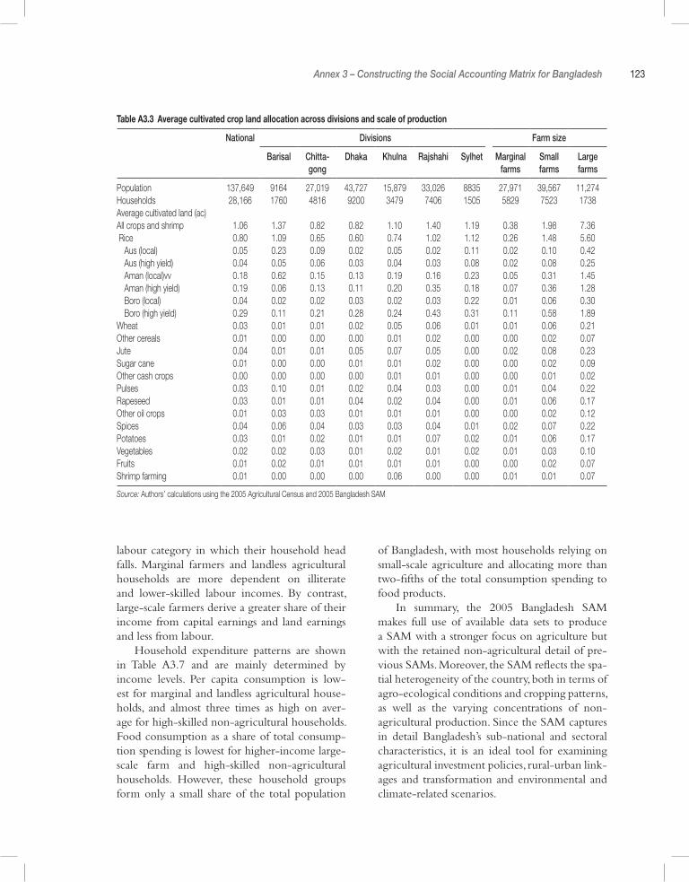
Annex 3 – Constructing the Social Accounting Matrix for Bangladesh 123
Table A3.3 Average cultivated crop land allocation across divisions and scale of production
National Divisions Farm size
Barisal Chitta-gong
Dhaka Khulna Rajshahi Sylhet Marginal farms
Small farms
Large farms
Population 137,649 9164 27,019 43,727 15,879 33,026 8835 27,971 39,567 11,274Households 28,166 1760 4816 9200 3479 7406 1505 5829 7523 1738Average cultivated land (ac)All crops and shrimp 1.06 1.37 0.82 0.82 1.10 1.40 1.19 0.38 1.98 7.36 Rice 0.80 1.09 0.65 0.60 0.74 1.02 1.12 0.26 1.48 5.60 Aus (local) 0.05 0.23 0.09 0.02 0.05 0.02 0.11 0.02 0.10 0.42 Aus (high yield) 0.04 0.05 0.06 0.03 0.04 0.03 0.08 0.02 0.08 0.25 Aman (local)vv 0.18 0.62 0.15 0.13 0.19 0.16 0.23 0.05 0.31 1.45 Aman (high yield) 0.19 0.06 0.13 0.11 0.20 0.35 0.18 0.07 0.36 1.28 Boro (local) 0.04 0.02 0.02 0.03 0.02 0.03 0.22 0.01 0.06 0.30 Boro (high yield) 0.29 0.11 0.21 0.28 0.24 0.43 0.31 0.11 0.58 1.89Wheat 0.03 0.01 0.01 0.02 0.05 0.06 0.01 0.01 0.06 0.21Other cereals 0.01 0.00 0.00 0.00 0.01 0.02 0.00 0.00 0.02 0.07Jute 0.04 0.01 0.01 0.05 0.07 0.05 0.00 0.02 0.08 0.23Sugar cane 0.01 0.00 0.00 0.01 0.01 0.02 0.00 0.00 0.02 0.09Other cash crops 0.00 0.00 0.00 0.00 0.01 0.01 0.00 0.00 0.01 0.02Pulses 0.03 0.10 0.01 0.02 0.04 0.03 0.00 0.01 0.04 0.22Rapeseed 0.03 0.01 0.01 0.04 0.02 0.04 0.00 0.01 0.06 0.17Other oil crops 0.01 0.03 0.03 0.01 0.01 0.01 0.00 0.00 0.02 0.12Spices 0.04 0.06 0.04 0.03 0.03 0.04 0.01 0.02 0.07 0.22Potatoes 0.03 0.01 0.02 0.01 0.01 0.07 0.02 0.01 0.06 0.17Vegetables 0.02 0.02 0.03 0.01 0.02 0.01 0.02 0.01 0.03 0.10Fruits 0.01 0.02 0.01 0.01 0.01 0.01 0.00 0.00 0.02 0.07Shrimp farming 0.01 0.00 0.00 0.00 0.06 0.00 0.00 0.01 0.01 0.07
Source: Authors’ calculations using the 2005 Agricultural Census and 2005 Bangladesh SAM
labour category in which their household head falls. Marginal farmers and landless agricultural households are more dependent on illiterate and lower-skilled labour incomes. By contrast, large-scale farmers derive a greater share of their income from capital earnings and land earnings and less from labour.
Household expenditure patterns are shown in Table A3.7 and are mainly determined by income levels. Per capita consumption is low-est for marginal and landless agricultural house-holds, and almost three times as high on aver-age for high-skilled non-agricultural households. Food consumption as a share of total consump-tion spending is lowest for higher-income large-scale farm and high-skilled non-agricultural households. However, these household groups form only a small share of the total population
of Bangladesh, with most households relying on small-scale agriculture and allocating more than two-fifths of the total consumption spending to food products.
In summary, the 2005 Bangladesh SAM makes full use of available data sets to produce a SAM with a stronger focus on agriculture but with the retained non-agricultural detail of pre-vious SAMs. Moreover, the SAM reflects the spa-tial heterogeneity of the country, both in terms of agro-ecological conditions and cropping patterns, as well as the varying concentrations of non-agricultural production. Since the SAM captures in detail Bangladesh’s sub-national and sectoral characteristics, it is an ideal tool for examining agricultural investment policies, rural-urban link-ages and transformation and environmental and climate-related scenarios.
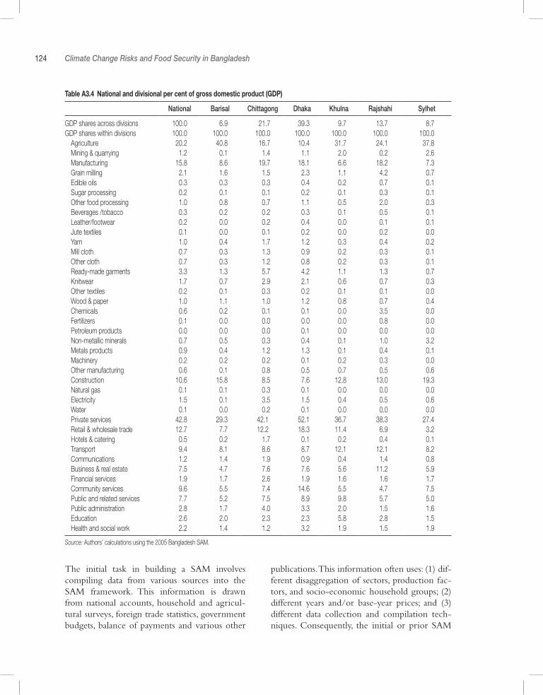
124 Climate Change Risks and Food Security in Bangladesh
Table A3.4 National and divisional per cent of gross domestic product (GDP)
National Barisal Chittagong Dhaka Khulna Rajshahi Sylhet
GDP shares across divisions 100.0 6.9 21.7 39.3 9.7 13.7 8.7GDP shares within divisions 100.0 100.0 100.0 100.0 100.0 100.0 100.0 Agriculture 20.2 40.8 16.7 10.4 31.7 24.1 37.8 Mining & quarrying 1.2 0.1 1.4 1.1 2.0 0.2 2.6 Manufacturing 15.8 8.6 19.7 18.1 6.6 18.2 7.3 Grain milling 2.1 1.6 1.5 2.3 1.1 4.2 0.7 Edible oils 0.3 0.3 0.3 0.4 0.2 0.7 0.1 Sugar processing 0.2 0.1 0.1 0.2 0.1 0.3 0.1 Other food processing 1.0 0.8 0.7 1.1 0.5 2.0 0.3 Beverages /tobacco 0.3 0.2 0.2 0.3 0.1 0.5 0.1 Leather/footwear 0.2 0.0 0.2 0.4 0.0 0.1 0.1 Jute textiles 0.1 0.0 0.1 0.2 0.0 0.2 0.0 Yarn 1.0 0.4 1.7 1.2 0.3 0.4 0.2 Mill cloth 0.7 0.3 1.3 0.9 0.2 0.3 0.1 Other cloth 0.7 0.3 1.2 0.8 0.2 0.3 0.1 Ready-made garments 3.3 1.3 5.7 4.2 1.1 1.3 0.7 Knitwear 1.7 0.7 2.9 2.1 0.6 0.7 0.3 Other textiles 0.2 0.1 0.3 0.2 0.1 0.1 0.0 Wood & paper 1.0 1.1 1.0 1.2 0.8 0.7 0.4 Chemicals 0.6 0.2 0.1 0.1 0.0 3.5 0.0 Fertilizers 0.1 0.0 0.0 0.0 0.0 0.8 0.0 Petroleum products 0.0 0.0 0.0 0.1 0.0 0.0 0.0 Non-metallic minerals 0.7 0.5 0.3 0.4 0.1 1.0 3.2 Metals products 0.9 0.4 1.2 1.3 0.1 0.4 0.1 Machinery 0.2 0.2 0.2 0.1 0.2 0.3 0.0 Other manufacturing 0.6 0.1 0.8 0.5 0.7 0.5 0.6 Construction 10.6 15.8 8.5 7.6 12.8 13.0 19.3 Natural gas 0.1 0.1 0.3 0.1 0.0 0.0 0.0 Electricity 1.5 0.1 3.5 1.5 0.4 0.5 0.6 Water 0.1 0.0 0.2 0.1 0.0 0.0 0.0 Private services 42.8 29.3 42.1 52.1 36.7 38.3 27.4 Retail & wholesale trade 12.7 7.7 12.2 18.3 11.4 6.9 3.2 Hotels & catering 0.5 0.2 1.7 0.1 0.2 0.4 0.1 Transport 9.4 8.1 8.6 8.7 12.1 12.1 8.2 Communications 1.2 1.4 1.9 0.9 0.4 1.4 0.8 Business & real estate 7.5 4.7 7.6 7.6 5.6 11.2 5.9 Financial services 1.9 1.7 2.6 1.9 1.6 1.6 1.7 Community services 9.6 5.5 7.4 14.6 5.5 4.7 7.5 Public and related services 7.7 5.2 7.5 8.9 9.8 5.7 5.0 Public administration 2.8 1.7 4.0 3.3 2.0 1.5 1.6 Education 2.6 2.0 2.3 2.3 5.8 2.8 1.5 Health and social work 2.2 1.4 1.2 3.2 1.9 1.5 1.9
Source: Authors’ calculations using the 2005 Bangladesh SAM.
The initial task in building a SAM involves compiling data from various sources into the SAM framework. This information is drawn from national accounts, household and agricul-tural surveys, foreign trade statistics, government budgets, balance of payments and various other
publications. This information often uses: (1) dif-ferent disaggregation of sectors, production fac-tors, and socio-economic household groups; (2) different years and/or base-year prices; and (3) different data collection and compilation tech-niques. Consequently, the initial or prior SAM
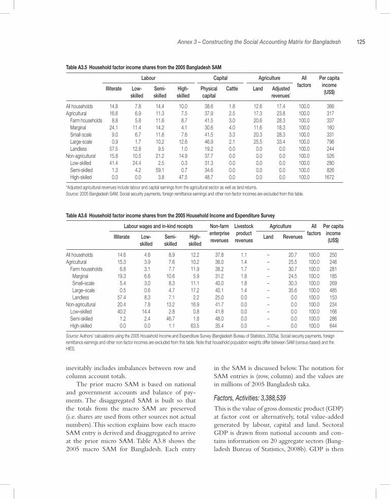
Annex 3 – Constructing the Social Accounting Matrix for Bangladesh 125
Table A3.5 Household factor income shares from the 2005 Bangladesh SAM
Labour Capital Agriculture All factors
Per capita income (US$)
Illiterate Low-skilled
Semi-skilled
High-skilled
Physical capital
Cattle Land Adjusted revenues*
All households 14.8 7.8 14.4 10.0 38.6 1.8 12.6 17.4 100.0 366Agricultural 16.6 6.9 11.3 7.5 37.9 2.5 17.3 23.8 100.0 317 Farm households 8.8 5.8 11.6 8.7 41.5 3.0 20.6 28.3 100.0 337 Marginal 24.1 11.4 14.2 4.1 30.6 4.0 11.6 18.3 100.0 160 Small-scale 9.0 6.7 11.6 7.6 41.5 3.3 20.3 28.3 100.0 331 Large-scale 0.9 1.7 10.2 12.6 46.9 2.1 25.5 33.4 100.0 796 Landless 57.5 12.8 9.5 1.0 19.2 0.0 0.0 0.0 100.0 244Non-agricultural 15.8 10.5 21.2 14.9 37.7 0.0 0.0 0.0 100.0 526 Low-skilled 41.4 24.4 2.5 0.3 31.3 0.0 0.0 0.0 100.0 280 Semi-skilled 1.3 4.2 59.1 0.7 34.6 0.0 0.0 0.0 100.0 826 High-skilled 0.0 0.0 3.8 47.5 48.7 0.0 0.0 0.0 100.0 1672
*Adjusted agricultural revenues include labour and capital earnings from the agricultural sector as well as land returns. Source: 2005 Bangladesh SAM. Social security payments, foreign remittance earnings and other non-factor incomes are excluded from this table.
Table A3.6 Household factor income shares from the 2005 Household Income and Expenditure Survey
Labour wages and in-kind receipts Non-farm enterprise revenues
Livestock product
revenues
Agriculture All factors
Per capita income (US$)
Illiterate Low- skilled
Semi- skilled
High-skilled
Land Revenues
All households 14.6 4.6 8.9 12.2 37.8 1.1 – 20.7 100.0 250Agricultural 15.3 3.9 7.6 10.2 36.0 1.4 – 25.5 100.0 246 Farm households 6.8 3.1 7.7 11.9 38.2 1.7 – 30.7 100.0 281 Marginal 19.3 6.6 10.6 5.9 31.2 1.8 – 24.5 100.0 185 Small–scale 5.4 3.0 8.3 11.1 40.0 1.8 – 30.3 100.0 269 Large–scale 0.5 0.6 4.7 17.2 40.1 1.4 – 35.6 100.0 485 Landless 57.4 8.3 7.1 2.2 25.0 0.0 – 0.0 100.0 153Non-agricultural 20.4 7.8 13.2 16.9 41.7 0.0 – 0.0 100.0 234 Low–skilled 40.2 14.4 2.8 0.8 41.8 0.0 – 0.0 100.0 166 Semi-skilled 1.2 2.4 46.7 1.8 48.0 0.0 – 0.0 100.0 286 High-skilled 0.0 0.0 1.1 63.5 35.4 0.0 – 0.0 100.0 644
Source: Authors’ calculations using the 2005 Household Income and Expenditure Survey (Bangladesh Bureau of Statistics, 2005a). Social security payments, foreign remittance earnings and other non-factor incomes are excluded from this table. Note that household population weights differ between SAM (census-based) and the HIES.
inevitably includes imbalances between row and column account totals.
The prior macro SAM is based on national and government accounts and balance of pay-ments. The disaggregated SAM is built so that the totals from the macro SAM are preserved (i.e. shares are used from other sources not actual numbers). This section explains how each macro SAM entry is derived and disaggregated to arrive at the prior micro SAM. Table A3.8 shows the 2005 macro SAM for Bangladesh. Each entry
in the SAM is discussed below. The notation for SAM entries is (row, column) and the values are in millions of 2005 Bangladesh taka.
Factors, Activities: 3,388,539This is the value of gross domestic product (GDP) at factor cost or alternatively, total value-added generated by labour, capital and land. Sectoral GDP is drawn from national accounts and con-tains information on 20 aggregate sectors (Bang-ladesh Bureau of Statistics, 2008b). GDP is then
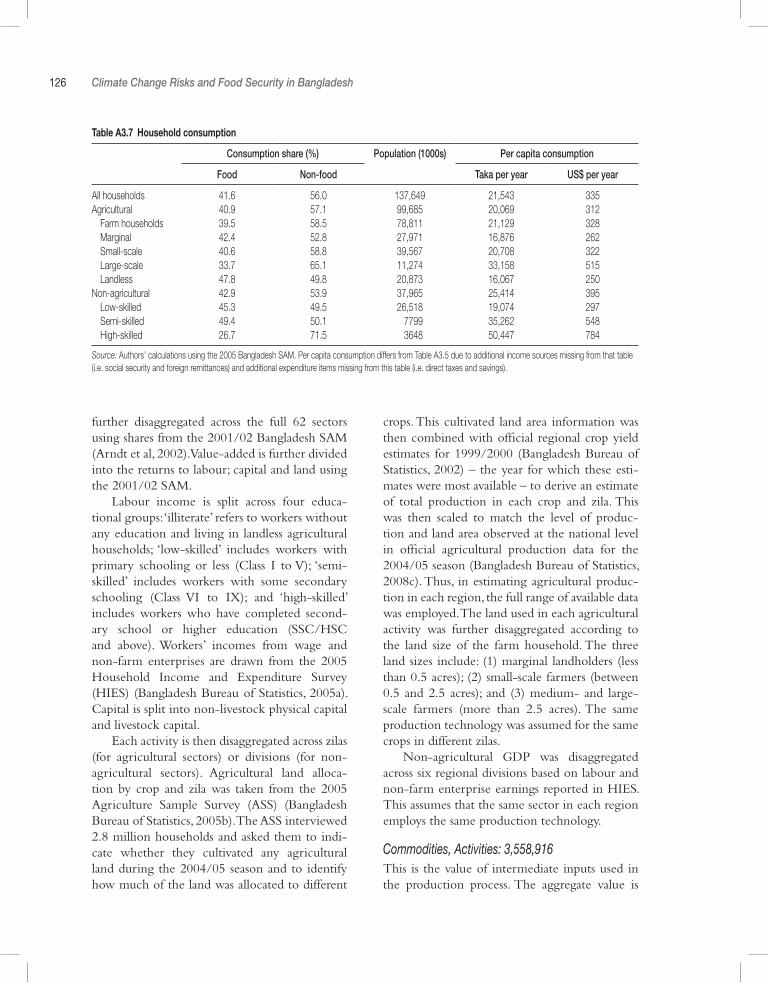
126 Climate Change Risks and Food Security in Bangladesh
Table A3.7 Household consumption
Consumption share (%) Population (1000s) Per capita consumption
Food Non-food Taka per year US$ per year
All households 41.6 56.0 137,649 21,543 335Agricultural 40.9 57.1 99,685 20,069 312 Farm households 39.5 58.5 78,811 21,129 328 Marginal 42.4 52.8 27,971 16,876 262 Small-scale 40.6 58.8 39,567 20,708 322 Large-scale 33.7 65.1 11,274 33,158 515 Landless 47.8 49.8 20,873 16,067 250Non-agricultural 42.9 53.9 37,965 25,414 395 Low-skilled 45.3 49.5 26,518 19,074 297 Semi-skilled 49.4 50.1 ,7799 35,262 548 High-skilled 26.7 71.5 ,3648 50,447 784
Source: Authors’ calculations using the 2005 Bangladesh SAM. Per capita consumption differs from Table A3.5 due to additional income sources missing from that table (i.e. social security and foreign remittances) and additional expenditure items missing from this table (i.e. direct taxes and savings).
further disaggregated across the full 62 sectors using shares from the 2001/02 Bangladesh SAM (Arndt et al, 2002). Value-added is further divided into the returns to labour; capital and land using the 2001/02 SAM.
Labour income is split across four educa-tional groups: ‘illiterate’ refers to workers without any education and living in landless agricultural households; ‘low-skilled’ includes workers with primary schooling or less (Class I to V); ‘semi-skilled’ includes workers with some secondary schooling (Class VI to IX); and ‘high-skilled’ includes workers who have completed second-ary school or higher education (SSC/HSC and above). Workers’ incomes from wage and non-farm enterprises are drawn from the 2005 Household Income and Expenditure Survey (HIES) (Bangladesh Bureau of Statistics, 2005a). Capital is split into non-livestock physical capital and livestock capital.
Each activity is then disaggregated across zilas (for agricultural sectors) or divisions (for non-agricultural sectors). Agricultural land alloca-tion by crop and zila was taken from the 2005 Agriculture Sample Survey (ASS) (Bangladesh Bureau of Statistics, 2005b). The ASS interviewed 2.8 million households and asked them to indi-cate whether they cultivated any agricultural land during the 2004/05 season and to identify how much of the land was allocated to different
crops. This cultivated land area information was then combined with official regional crop yield estimates for 1999/2000 (Bangladesh Bureau of Statistics, 2002) – the year for which these esti-mates were most available – to derive an estimate of total production in each crop and zila. This was then scaled to match the level of produc-tion and land area observed at the national level in official agricultural production data for the 2004/05 season (Bangladesh Bureau of Statistics, 2008c). Thus, in estimating agricultural produc-tion in each region, the full range of available data was employed. The land used in each agricultural activity was further disaggregated according to the land size of the farm household. The three land sizes include: (1) marginal landholders (less than 0.5 acres); (2) small-scale farmers (between 0.5 and 2.5 acres); and (3) medium- and large-scale farmers (more than 2.5 acres). The same production technology was assumed for the same crops in different zilas.
Non-agricultural GDP was disaggregated across six regional divisions based on labour and non-farm enterprise earnings reported in HIES. This assumes that the same sector in each region employs the same production technology.
Commodities, Activities: 3,558,916This is the value of intermediate inputs used in the production process. The aggregate value is

Tabl
e A3
.8 2
005
mac
ro S
AM fo
r Ban
glad
esh
(milli
ons
of Ta
ka)
Activ
ities
Com
mod
ities
Fact
ors
Hous
ehol
dsGo
vern
men
tTa
xes
Inve
stm
ent
Rest
of W
orld
Tota
l
Activ
ities
6,94
7,45
4
Com
mod
ities
3,55
8,91
62,
892,
513
206,
985
777,
864
613,
880
3,55
8,91
6
Fact
ors
3,38
8,53
93,
388,
539
Hous
ehol
ds3,
300,
422
109,
625
226,
043
Gove
rnm
ent
364,
169
25,8
37
Taxe
s24
3,19
649
,772
71,2
01
Savin
gs67
2,37
573
,396
32,0
94
Rest
of W
orld
859,
508
38,3
45
Tota
l6,
947,
454
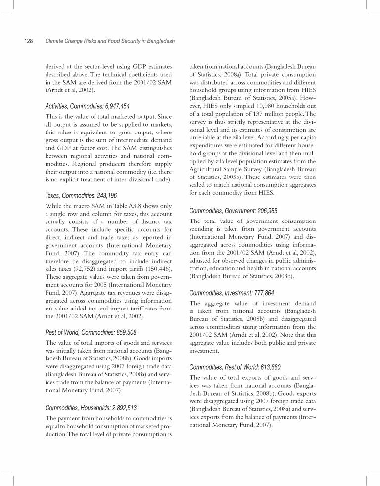
128 Climate Change Risks and Food Security in Bangladesh
derived at the sector-level using GDP estimates described above. The technical coefficients used in the SAM are derived from the 2001/02 SAM (Arndt et al, 2002).
Activities, Commodities: 6,947,454This is the value of total marketed output. Since all output is assumed to be supplied to markets, this value is equivalent to gross output, where gross output is the sum of intermediate demand and GDP at factor cost. The SAM distinguishes between regional activities and national com-modities. Regional producers therefore supply their output into a national commodity (i.e. there is no explicit treatment of inter-divisional trade).
Taxes, Commodities: 243,196While the macro SAM in Table A3.8 shows only a single row and column for taxes, this account actually consists of a number of distinct tax accounts. These include specific accounts for direct, indirect and trade taxes as reported in government accounts (International Monetary Fund, 2007). The commodity tax entry can therefore be disaggregated to include indirect sales taxes (92,752) and import tariffs (150,446). These aggregate values were taken from govern-ment accounts for 2005 (International Monetary Fund, 2007). Aggregate tax revenues were disag-gregated across commodities using information on value-added tax and import tariff rates from the 2001/02 SAM (Arndt et al, 2002).
Rest of World, Commodities: 859,508The value of total imports of goods and services was initially taken from national accounts (Bang-ladesh Bureau of Statistics, 2008b). Goods imports were disaggregated using 2007 foreign trade data (Bangladesh Bureau of Statistics, 2008a) and serv-ices trade from the balance of payments (Interna-tional Monetary Fund, 2007).
Commodities, Households: 2,892,513The payment from households to commodities is equal to household consumption of marketed pro-duction. The total level of private consumption is
taken from national accounts (Bangladesh Bureau of Statistics, 2008a). Total private consumption was distributed across commodities and different household groups using information from HIES (Bangladesh Bureau of Statistics, 2005a). How-ever, HIES only sampled 10,080 households out of a total population of 137 million people. The survey is thus strictly representative at the divi-sional level and its estimates of consumption are unreliable at the zila level. Accordingly, per capita expenditures were estimated for different house-hold groups at the divisional level and then mul-tiplied by zila level population estimates from the Agricultural Sample Survey (Bangladesh Bureau of Statistics, 2005b). These estimates were then scaled to match national consumption aggregates for each commodity from HIES.
Commodities, Government: 206,985The total value of government consumption spending is taken from government accounts (International Monetary Fund, 2007) and dis-aggregated across commodities using informa-tion from the 2001/02 SAM (Arndt et al, 2002), adjusted for observed changes in public adminis-tration, education and health in national accounts (Bangladesh Bureau of Statistics, 2008b).
Commodities, Investment: 777,864The aggregate value of investment demand is taken from national accounts (Bangladesh Bureau of Statistics, 2008b) and disaggregated across commodities using information from the 2001/02 SAM (Arndt et al, 2002). Note that this aggregate value includes both public and private investment.
Commodities, Rest of World: 613,880The value of total exports of goods and serv-ices was taken from national accounts (Bangla-desh Bureau of Statistics, 2008b). Goods exports were disaggregated using 2007 foreign trade data (Bangladesh Bureau of Statistics, 2008a) and serv-ices exports from the balance of payments (Inter-national Monetary Fund, 2007).
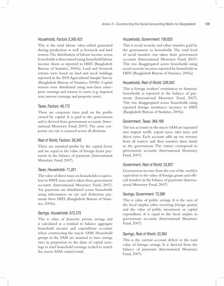
Annex 3 – Constructing the Social Accounting Matrix for Bangladesh 129
Households, Factors 3,300,422This is the total labour value-added generated during production as well as livestock and land returns. The distribution of labour income across households is determined using household labour income shares as reported in HIES (Bangladesh Bureau of Statistics, 2005a). Land and livestock returns were based on land and stock holdings reported in the 2005 Agricultural Sample Survey (Bangladesh Bureau of Statistics, 2005b). Capital returns were distributed using non-farm enter-prise earnings and returns to assets (e.g. imputed rent, interest earnings and property rents).
Taxes, Factors: 49,772These are corporate taxes paid on the profits earned by capital. It is paid to the government and is derived from government accounts (Inter-national Monetary Fund, 2007). The same cor-porate tax rate is assumed across all divisions.
Rest of World, Factors: 38,345These are remitted profits by the capital factor and are equal to the value of foreign factor pay-ments in the balance of payments (International Monetary Fund, 2007).
Taxes, Households: 71,201The value of direct taxes on households is equiva-lent to PAYE taxes and is taken from government accounts (International Monetary Fund, 2007). Tax payments are distributed across households using information on tax and deduction pay-ments from HIES (Bangladesh Bureau of Statis-tics, 2005a).
Savings, Households: 672,375This is value of domestic private savings and is calculated as a residual to balance aggregate household income and expenditure accounts when constructing the macro SAM. Household groups in the SAM are assumed to have savings rates in proportion to the share of capital earn-ings in total household earnings (scaled to match the macro SAM control total).
Households, Government: 109,625This is social security and other transfers paid by the government to households. The total level of social transfers was taken from government accounts (International Monetary Fund, 2007). This was disaggregated across households using social security incomes reported by households in HIES (Bangladesh Bureau of Statistics, 2005a).
Households, Rest of World: 226,043This is foreign workers’ remittances to domestic households as reported in the balance of pay-ments (International Monetary Fund, 2007). This was disaggregated across households using reported foreign remittance incomes in HIES (Bangladesh Bureau of Statistics, 2005a).
Government, Taxes: 364,169The tax accounts in the micro SAM are separated into import tariffs, export taxes, sales taxes and direct taxes. Each account adds up tax revenue from all sources and then transfers these funds to the government. The entries correspond to government accounts (International Monetary Fund, 2007).
Government, Rest of World: 25,837Government income from the rest of the world is equivalent to the value of foreign grants and offi-cial transfers in the balance of payments (Interna-tional Monetary Fund, 2007).
Savings, Government: 73,396This is value of public savings. It is the sum of the fiscal surplus (after receiving foreign grants) and the value of public investment or capital expenditure. It is equal to the fiscal surplus in government accounts (International Monetary Fund, 2007).
Savings, Rest of World: 32,094This is the current account deficit or the total value of foreign savings. It is derived from the balance of payments (International Monetary Fund, 2007).
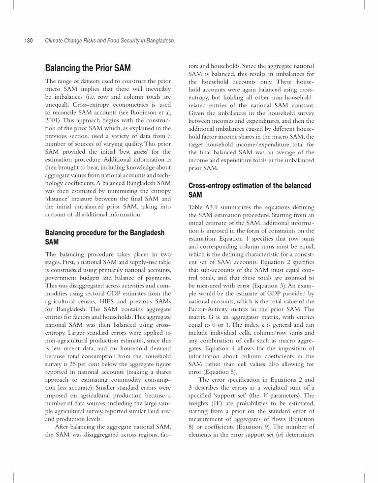
130 Climate Change Risks and Food Security in Bangladesh
Balancing the Prior SAMThe range of datasets used to construct the prior micro SAM implies that there will inevitably be imbalances (i.e. row and column totals are unequal). Cross-entropy econometrics is used to reconcile SAM accounts (see Robinson et al, 2001). This approach begins with the construc-tion of the prior SAM which, as explained in the previous section, used a variety of data from a number of sources of varying quality. This prior SAM provided the initial ‘best guess’ for the estimation procedure. Additional information is then brought to bear, including knowledge about aggregate values from national accounts and tech-nology coefficients. A balanced Bangladesh SAM was then estimated by minimizing the entropy ‘distance’ measure between the final SAM and the initial unbalanced prior SAM, taking into account of all additional information.
Balancing procedure for the Bangladesh SAM
The balancing procedure takes places in two stages. First, a national SAM and supply-use table is constructed using primarily national accounts, government budgets and balance of payments. This was disaggregated across activities and com-modities using sectoral GDP estimates from the agricultural census, HIES and previous SAMs for Bangladesh. The SAM contains aggregate entries for factors and households. This aggregate national SAM was then balanced using cross-entropy. Larger standard errors were applied to non-agricultural production estimates, since this is less recent data, and on household demand because total consumption from the household survey is 25 per cent below the aggregate figure reported in national accounts (making a shares approach to estimating commodity consump-tion less accurate). Smaller standard errors were imposed on agricultural production because a number of data sources, including the large sam-ple agricultural survey, reported similar land area and production levels.
After balancing the aggregate national SAM, the SAM was disaggregated across regions, fac-
tors and households. Since the aggregate national SAM is balanced, this results in imbalances for the household accounts only. These house-hold accounts were again balanced using cross-entropy, but holding all other non-household-related entries of the national SAM constant. Given the imbalances in the household survey between incomes and expenditures, and then the additional imbalances caused by different house-hold factor income shares in the macro SAM, the target household income/expenditure total for the final balanced SAM was an average of the income and expenditure totals in the unbalanced prior SAM.
Cross-entropy estimation of the balanced SAM
Table A3.9 summarizes the equations defining the SAM estimation procedure. Starting from an initial estimate of the SAM, additional informa-tion is imposed in the form of constraints on the estimation. Equation 1 specifies that row sums and corresponding column sums must be equal, which is the defining characteristic for a consist-ent set of SAM accounts. Equation 2 specifies that sub-accounts of the SAM must equal con-trol totals, and that these totals are assumed to be measured with error (Equation 3). An exam-ple would be the estimate of GDP provided by national accounts, which is the total value of the Factor-Activity matrix in the prior SAM. The matrix G is an aggregator matrix, with entries equal to 0 or 1. The index k is general and can include individual cells, column/row sums and any combination of cells such as macro aggre-gates. Equation 4 allows for the imposition of information about column coefficients in the SAM rather than cell values, also allowing for error (Equation 5).
The error specification in Equations 2 and 3 describes the errors as a weighted sum of a specified ‘support set’ (the V parameters). The weights (W ) are probabilities to be estimated, starting from a prior on the standard error of measurement of aggregates of flows (Equation 8) or coefficients (Equation 9). The number of elements in the error support set (w) determines
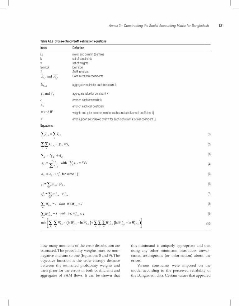
Annex 3 – Constructing the Social Accounting Matrix for Bangladesh 131
how many moments of the error distribution are estimated. The probability weights must be non-negative and sum to one (Equations 8 and 9). The objective function is the cross-entropy distance between the estimated probability weights and their prior for the errors in both coefficients and aggregates of SAM flows. It can be shown that
this minimand is uniquely appropriate and that using any other minimand introduces unwar-ranted assumptions (or information) about the errors.
Various constraints were imposed on the model according to the perceived reliability of the Bangladesh data. Certain values that appeared
Table A3.9 Cross-entropy SAM estimation equations
Index Definition
i, j row (i) and column (j) entriesk set of constraintsw set of weightsSymbol DefinitionT
i,jSAM in values
, , and i j i jA A SAM in column coefficients
, ,k i jG aggregator matrix for each constraint k
and k kγ γ aggregate value for constraint k
ek
error on each constraint k
,Ai je error on each cell coefficient
and W W weights and prior on error term for each constraint k or cell coefficient i,j
V error support set indexed over w for each constraint k or cell coefficient i,j
Equations
, ,i j i ji j
T T =∑ ∑ (1)
, , i, jk i j ki j
G = T γ⋅∑∑ (2)
k kk eγ γ= + (3)
with i, ji, ji, j
i, j ii
T = = 1 iA AT
∀∑∑ (4)
, , , for some i, jAi j i j i jA A e= + (5)
k k, w k, ww
= e W V⋅∑ (6)
, , , , ,A A Ai j i j w i j w
w
e = W V ⋅∑ (7)
, ,k w k ww
W = 1 with 0 W 1≤ ≤∑ (8)
, , , ,A A
i j w i j ww
W = 1 with 0 W 1≤ ≤∑ (9)
( ) ( ), , , , , , , , ,min ln ln ln lnA A Ak w k w k w i j w i j w i j w
k w i j w
W W W W W W
⋅ − + − ∑ ∑ ∑∑∑ (10)
and
and
and
132 Climate Change Risks and Food Security in Bangladesh
in national accounts were maintained in order to remain consistent with the overall macro structure of the economy. The macro-economic aggregates that were maintained in the micro-SAM include: total labour value-added; total capital value-added; household final demand; government spending; investment demand; exports; imports; government borrowing/saving; current account balance; sales taxes; import tariffs; direct taxes on enterprises; government transfers to enterprises; enterprise transfers to the rest of the world; enter-prise transfers to government; household trans-fers to government; government transfers to the rest of the world; and household foreign transfers received. Since the household survey (HIES) and the agricultural production and GDP estimates from national accounts were taken from data for the same year, the standard errors applied to the various components were uniform.
Notes1 For general discussions of SAMs see Pyatt
and Round (1985) and Reinert and Roland-Holst (1997); for perspectives on SAM-based modelling see Pyatt (1988) and Robinson and Roland-Holst (1988).
2 Note that ‘low-skilled non-agricultural’ households include both household heads who are illiterate and those who completed some level of primary schooling
3 There are differences in the interpretation of factor income sources in the SAM and survey. The SAM separates land returns from agri-cultural labour and capital earnings, while the HIES reports agricultural revenues after subtracting production costs (i.e. returns to all agricultural factors). Survey agricultural income shares are therefore larger than land returns in the SAM. Similarly, non-farm enterprise earnings are a form of ‘mixed income’. In other words, they include both labour and capital earnings, and are therefore typically higher than capital earnings alone.
References
Adger, W. N., Agrawala, S., Mirza, M.M.Q., Conde, C., O’Brien, K., Pulhin, J., Pulwarty, R., Smit, B. and Takahashi, K. (2007) ‘Assessment of adaptation prac-tices, options, constraints and capacity’ in Parry, M. L., Canziani, O. F., Palutikof, J. P., van der Linden, P. J. and Hanson, C. E. (eds) Climate Change 2007: Impacts, Adaptation and Vulnerability. Contribution of Working Group II to the Fourth Assessment Report of the Intergovernmental Panel on Climate Change, Cambridge University Press, Cambridge, UK, pp717–743
Adler, R. F., Huffman, G. J. and Keehn, P. R. (1994) ‘Global rain estimates from microwave adjusted geosynchronous IR data’, Remote Sensing Review, vol 11, pp125–52
Aerts, J. C. J. H., De Vente, J., Hassan, A. and Martin T. C. (2000) Spatial Integration of Hydrological Monitoring and Remote Sensing Applications (SPIHRAL), Final Report, Resource Analysis, Delft, Netherlands
Agrawala, S., Ota, T., Ahmed, A. U., Smith, J. and van Aalst, M. (2003) Development and Climate Change in Bangladesh: Focus on Coastal Flooding and the Sundar-bans, Environment Directorate and Developmental Co-operation Directorate, Organization for Eco-nomic Co-operation and Development, Paris
Ahmad, A. S. M. S., Munim, A. A., Begum, Q. N. and Choudhury, A. M. (1996) ‘El Nino-southern oscilla-tion and rainfall variation over Bangladesh’, Mausam, vol 47, no 2, pp157–62
Ahmed, A. U. and Mirza, M. M. Q. (2000) ‘Review of causes and dimensions of floods with particular ref-erence to flood ’98: national perspectives’ in Ahmad, Q. K., Chowdhury, A. K. A., Imam, S. H. and Sarker, M. (eds) Perspectives on Flood 1998, University Press Ltd, Dhaka, pp67–84
Ahmed, A. U. (2006) Bangladesh: Climate Change Impacts and Vulnerability, Climate Change Cell, Bangladesh, p42
Ainsworth, E.A., Leakey, A.D.B., Ort, D.R. and Long, S.P. (2008) ‘FACE-ing the facts: Inconsistencies and interdependence among field, chamber and mode-
ling studies of elevated [CO2] impacts on crop yield and food supply’, New Phytologist, 5pp
Alley, R. B., Clark, P. U., Huybrechts, P. and Joughin, I. (2005) ‘Ice-sheet and sea level changes’, Science, vol 310, pp456–460
Ali, A. (1999) ‘Climate change impacts and adaptation assessment in Bangladesh’, Climate Research, vol 12, pp109–116
Ali, A. (2006) ‘Mathematically predicting the impacts of climate change and sea level rise on storm surges in the Bangladesh coastal region’, presented at the Workshop on Climate Change Impact Modelling, Climate Change Cell, Department of Environment, Government of the People’s Republic of Bangla-desh, Dhaka, 26–27 February
Arndt, C., Dorosh, P., Fontana, M. and Zohir, S. (2002) Opportunities and Challenges in Agriculture and Gar-ments: A General Equilibrium Analysis of the Bangladesh Economy, TMD Discussion Paper no 107, IFPRI, Washington D.C.
Bangladesh Bureau of Statistics (BBS) (1998) Agricul-tural Statistical Year Book of Bangladesh, Dhaka, Bang-ladesh
BBS (2002) Regional Estimates of Agricultural Crop Produc-tion: 1985/86-1999/2000, Dhaka, Bangladesh
BBS (2005a) Household Income and Expenditure Survey 2004, Dhaka, Bangladesh
BBS (2005b) Agriculture Sample Survey 2005, Dhaka, Bangladesh
BBS (2006a) Agriculture Sample Survey of Bangladesh, Dhaka, Bangladesh
BBS (2006b) Report of the Household Income and Expendi-ture Survey, Dakha, Bangladesh
BBS (2008a) Foreign Trade Statistics, Dhaka, Bangladesh, available at www.bbs.gov.bd
BBS (2008b) National Accounts 2005, Dhaka, Bangla-desh, available at www.bbs.gov.bd
BBS (2008c) Handbook of Agricultural Statistics 2007, Dhaka, Bangladesh, available at www.bbs.gov.bd
134 Climate Change Risks and Food Security in Bangladesh
BBS (2009) National Accounts 2009, Dhaka, BangladeshBCA (2002) Bangladesh Country Almanac, available at
www.cimmyt.org/bangladesh/Programs/Program4.htm
Bangladesh University of Engineering and Technology (1993) Multipurpose Cyclone Shelter Programme, Final Report, UNDP/World Bank, Dhaka, Bangladesh
Brammer, H. (1996) The Geography of the Soils of Bangla-desh, University Press, Dhaka, Bangladesh, 287pp
BRRI (Bangladesh Rice Research Institute) (2007) Modern Rice Cultivation, Bangladesh Rice Research Institute, Joydebpur, Bangladesh, 66pp
CEGIS (2006) Impacts of Sea Level Rise on Land-use Suitability and Adaptation Options, Draft Final Report, Submitted to the Ministry of Environment and For-est, Government of Bangladesh and United Nations Development Programme (UNDP), Dhaka, Bang-ladesh
CEGIS (2009), image courtesy of Maminul Haque Sarker at CEGIS, appears in ‘Where warming hits hard’, Nature Reports – Climate Change, 15 January 2009
Chen, J., Lin, H. and Pei, Z. (2007) ‘Application of ENVISAT ASAR data in mapping rice crop growth in Southern China’ Geoscience and Remote Sensing Letters, IEEE, vol 4, no 3, pp431–435, Doi: 10.1109/LGRS.2007.896996
Chowdhury, M. R. (2000) ‘An assessment of flood forecasting in Bangladesh: The experience of the 1998 flood’, Natural Hazards, vol 22, pp139–163
Chowdhury, M. R. (2003) ‘The El Nino-Southern Oscillation (ENSO) and seasonal flooding – Bangla-desh’, Theoretical Applied Climatology, vol 76, pp105–24
Chowdhury, J. A. and co-editors (2005c) Yearbook of Agricultural Statistics of Bangladesh, Bangladesh Bureau of Statistics, Dhaka, Bangladesh, p344
Cline, W. (2007) Global Warming and Agriculture – Impact Estimates by Country, Center for Global Develop-ment, Peterson Institute, Washington D.C, p186
Copenhagen Diagnosis (2009) Updating the World on the Latest Climate Science, University of New South Wales Climate Change Research Centre (CCRC), Sydney, Australia, p60
Cuny, F. C. (1983) Disasters and Development, Oxford University Press, New York
Dervis, K., de Melo, J. and Robinson, S. (1982) General Equilibrium Models for Development Policy, Cambridge University Press, New York
Dyurgerov, M. D. and Meier, M. F. (2005) Glaciers and Changing Earth System: A 2004 Snapshot, Institute of Arctic and Alpine Research, University of Colorado, Boulder, CO, p117
Easterling, W. E., Aggarwal, P. K., Batima, P., Brander, K. M., Erda, L., Howden, S. M., Kirilenko, A., Mor-ton, J., Soussana, J.-F., Schmidhuber, J. and Tubiello, F. N. (2007) ‘Food, fibre and forest products’, in M. L. Parry, O. F. Canziani, J. P. Palutikof, P. J. van der Linden and C. E. Hanson (Eds) Climate Change 2007: Impacts, Adaptation and Vulnerability, Contribu-tion of Working Group II to the Fourth Assessment Report of the Intergovernmental Panel on Climate Change, Cambridge University Press, Cambridge, UK, pp273–313
Faisal, I. M. and Parveen, S. (2003) ‘Food security in the face of climate change, population growth, and resource constraints: Implications for Bangladesh’, Environmental Management, vol 34, no 4, pp487–98
Farr, T. G. et al (2007), ‘The Shuttle Radar Topography Mission’, Review of Geophysics, vol 45
Fischer, G., Shah, M. and van Velthuizen, H. (2002) Climate Change and Agricultural Vulnerability, Inter-national Institute for Applied Systems Analysis, Lax-enburg, Austria, p152
Food and Agriculture Organization of the United Nations (2008). FAOSTAT, Rome, available at www.fao.org
Gomosta, A. R., Quayyum, H. A. and Mahbub, A. A. (2001) ‘Tillering duration and yielding ability of rice varieties in the winter rice season of Bangla-desh’, in Peng, S. and Hardy, B. (eds) Rice Research for Food Security and Poverty Alleviation, International Rice Research Institute, Philippines, 692pp
Goodbred, S. L. and Kuehl, S. A. (2000) ‘Enormous Ganges-Brahmaputra sediment discharge during strengthened early Holocene monsoon’, Geology, vol 28, no 12, December, pp1083–86
Habibullah, M., Ahmed, A.U. and Karim, Z. (1998) ‘Assessment of Foodgrain Production Loss Due to Climate Induced Enhanced Soil Salinity’ in Huq, S., Karim, Z., Asaduzzaman, M. and Mahtab, F. (eds) Vulnerability and Adaptation to Climate Change for Bangladesh,Kluwer Academic Publishers, Dordrecht, pp55–70
Hassan, A. (2006). ‘Recent trends in Bangladesh (tech-nical notes)’, Centre for Environmental and Geo-graphical Information Services (CEGIS), Dhaka, Bangladesh
Hassan, A. and Shah, M. A. R. (2006) ‘Impacts of sea level rise on suitability of agriculture and fisheries: A case study on southwest region of Bangladesh’, pre-sented in the Workshop on Climate Change Impact Modelling, Climate Change Cell, Department of Environment, Government of Bangladesh, Dhaka, 26–27 February
References 135
Hassan, A., Chowdhury, E. H. and Khatun, M. F. (2007) Classification of Flood for Seasonal Flood Management, paper presented on International Conference on Water & Flood Management – 2007, Dhaka, Bang-ladesh
Hatfield, J., Boote, K., Fay, P., Hahn, L., Izaurralde, C., Kimball, B. A., Mader, T., Morgan, J., Ort, D., Pol-ley, W., Thomson, A., Wolfe, D., (2008) ‘Agriculture’, Chapter 2 in The effects of climate change on agricul-ture, land resources, water resources, and biodiversity in the United States, a report by the U.S. Climate Change Science Program and the Subcommittee on Global Change Research, Washington, DC, 362pp
Haque, C. E. (1997) Hazards in a Fickle Environment: Bangladesh, Kluwer Academic Publishers, Dordrecht
Hendry, G. R., and Kimball, B. A. (1994) ‘The FACE Programme’, Agriculture and Forest Meteorology, vol 70, pp3–14
Hofer, T. and Messerli, B. (2007) Floods in Bangladesh – History, Dynamics and Rethinking the Role of the Himalayas, United Nations University Press, Tokyo, New York, Paris, p468
Hoogenboom G., Jones, J. W., Porter, C. H., Wilkens, P. W., Boote, K. J., Batchelor, W. D., Hunt, L. A. and Tsuji, G. Y. (2003) DSSAT v4 vol. 1, University of Hawaii, Honolulu, HI
Hopson, T. and Webster, P. (2007) ‘A 1–10 day ensem-ble forecasting scheme for the major river basins of Bangladesh: forecasting severe floods of 2003–2007’, Journal of Hydrometeorology, in press.
Horton, R., Herweijer, C., Rosenzweig, C., Liu, J. P., Gornitz, V. and Ruane, A. C. (2008) ‘Sea level rise projections for current generation CGCMs based on the semi-empirical method’, Geophysi-cal Research Letters, vol 35, L02715, doi:10.1029/2007GL032486
Huq, S., Karim, Z., Asaduzzaman, M. and Mahtab, F. (eds) (1999) Vulnerability and Adaptation to Climate Change in Bangladesh, Kluwer Academic Publishers, Dordrecht, Netherlands
Hussain, S. G. (1995) ‘Decision support system for assessing rice yield losses from annual flooding in Bangladesh’, dissertation submitted to the Graduate Division of the University of Hawaii, p137
Hussain, S. G. (2006) Agriculture Water Demand and Drought Modeling, Proceedings of Workshop on Cli-mate Change Impact Modeling, Climate Change Cell, Department of Environment, Government of the People’s Republic of Bangladesh, Dhaka
International Monetary Fund (2007) Bangladesh: Statis-tical Appendix, Country Report No. 07/229, Wash-ington D.C.
IPCC (2001) Climate Change 2001: The Scientific Basis, Contribution of Working Group I to the Third Assessment Report of the Intergovernmental Panel on Climate Change, Cambridge University Press, Cambridge, UK
IPCC (2007a) Climate Change 2007: The Scientific Basis, Contribution of Working Group I to the Fourth Assessment Report of the Intergovernmental Panel on Climate Change, Solomon, S., et al (eds), Cam-bridge University Press, Cambridge, UK
IPCC (2007b) Climate Change 2007: Impacts, Adap-tation and Vulnerability, Contribution of Working Group II to the Fourth Assessment Report of the Intergovernmental Panel on Climate Change, Parry, M., et al (eds), Cambridge University Press, Cam-bridge, UK
Islam, M. N., Mannan, M. A., Devkota, L. P. and Nessa, M. (2005) Validation of PRECIS Regional Climate Model in Bangladesh, Climate Change Cell, Bangla-desh, Dhaka, p46
IWM and CEGIS (2007), Investigating the Impact of Rel-ative Sea level Rise on Coastal Communities and their Livelihoods in Bangladesh, Final Report, June 2007, IWM /CEGIS/Government of Bangladesh, Dhaka
Jianchu, X., Shrestha, A., Vaidya, R., Eriksson, M., Hewitt, K. (2007) ‘The Melting Himalayas: Regional Challenges and Local Impacts of Climate Change on Mountain Ecosystems and Livelihoods’, ICI-MOD Technical Paper, June, 24pp
Jones, J., Hoogenboom, W. G., Porter, C. H., Boote, K. J., Batchelor, W. D., Hunt, L.A., Wilkens, P. W., Singh, U., Gijsman, A. J. and Ritchie, J. T. (2003) ‘The DSSAT cropping system model’, European Journal of Agronomy, vol 18, nos 3–4, pp235–65
Joyce, R. J., Janowiak, J. E., Arkin, P. A. and Xie, P. (2004) ‘CMORPH: A method that produces global precipitation estimates from passive microwave and infrared data at high spatial and temporal resolution’, Journal of Hydrometeorology, vol 5, pp487–503
Kanamitsu, M., Ebisuzaki, W., Woollen, J., Yang, S.-K., Hnilo, J., Fiorino, M. and Potter, J. (2002) ‘NCEP/DOE AMIP-II Reanalysis (R-2)’, Bulletin of the American Meteorology Society, vol 83, no 7, pp1019–37
Karim, Z., Ahmed, M., Hussain, S.G. and Rashid, Kh. B. (1994) ‘Impact of climate change on the produc-tion of modern rice in Bangladesh’, Implications of Climate Change for International Agriculture: Crop Mod-eling Study, US Environmental Protection Agency, Washington D.C.
Karim, Z., Hussain, S.G. and Ahmed, M. (1996) ‘Assess-ing impacts of climate variation on foodgrain pro-duction in Bangladesh’, Journal of Water, Air and Soil Pollution, vol 92, pp53–62
136 Climate Change Risks and Food Security in Bangladesh
Karim, Z., Hussain, S. G. and Ahmed, A. U. (1998), ‘Climate change vulnerability of crop agriculture’, in S. Huq, Z. Karim, M. Asaduzaman and F. Mahtab (eds), Vulnerability and Adaptation to Climate Change for Bangladesh, Kluwer Academic Publishers, Dor-drecht, , Netherlands, pp39–54
Khalil, G. M. (1990) ‘Flood in Bangladesh: a ques-tion of disciplining the river’, Natural Hazards vol 3, pp379–401
Kimball, B. A. and Bernacchi, C. J. (2006) ‘Evapo-transpiration, canopy temperature, and plant water relations’ in Managed Ecosystems and CO
2: Case Stud-
ies, Processes, and Perspectives. Springer-Verlag, Berlin, Germany, pp311–324
Kotera, A., and Nawata, E. (2007) ‘Role of plant height in the submergence tolerance of rice: A simulation analysis using an empirical model’, Agricultural Water Management, vol 89, pp49–58
Lal, M., Meehl, G. A., and Arblaster, J. M. (1998a) ‘Sim-ulation of Indian Summer Monsoon Rainfall and its Intraseasonal Variability in NCAR’s Climate System Model’, National Center for Atmospheric Research, draft, Boulder, CO
Lal, M., Singh, K. K., Raghore, L. S., Srinivasan, G., and Saseendran, S. A. (1998b) ‘Vulnerability of Rice and Wheat Yields in NW India to Future Changes in Climate’, Agriculture and Forest Meteorology, vol 89, pp101–114
Lal, M., Singh, K. K., Srinivasan, G., Rathore, L. S. and Mall, R. K. (1998c) ‘Growth and Yield Responses of Soybean in Madya Pradesh, India to Climate Variability and Change’, submitted to Agriculture and Forest Mete-orology, Indian Institute for Technology, New Delhi
Latif, M. A., Islam, M. R., Ali, M. Y. and Saleque, M. A. (2005) ‘Validation of the system of rice intensifica-tion (SRI) in Bangladesh’, Field Crops Research, vol 93, pp281–292
Long, S. P., Ainsworth, E., Leakey, A. and Morgan, P. (2005) ‘Global food insecurity: Treatment of major food crops with elevated carbon dioxide or ozone under large-scale fully open-air conditions suggests recent models may have overestimated future yields’, Philosophical Transactions of the Royal Society B, vol 360, pp2011–20
Long, S. P., Ainsworth, E. A., Leakey, A. D. B. (2006) ‘Food for thought: lower-than-expected crop yield stimulation with rising CO
2 concentrations’, Science,
vol 312, pp1918–1921Mahmood, R. (1997) ‘Impacts of air temperature vari-
ations on the boro rice phenology in Bangladesh: implications for irrigation requirements’, Agricultural and Forest Meteorology, vol 84, pp233–247
Mahmood, R., Meo, M., Legates, D.R. and Morris-sey, M.L. (2003) ‘The CERES-Rice model-based estimates of potential monsoon season rainfed rice productivity in Bangladesh’, Professional Geographer, vol 55, no 2, pp269–73
Meehl, G.A., Covey, C., Delworth, T., Latif, M., McAv-aney, D., Mitchell, J.P.B., Stouffer, R.J. and Taylor, K.E. (2007) The WCRP CMIP3 multi-modal data-set: A new era in climate change research, Bulletin of the American Meteorological Society, vol 88, pp1383–1394
Mendelsohn, R. and Schlesinger, M. (1999) ‘Climate response functions’, Ambio, vol 28, no 4, pp362–66
Mirza, M. M. Q. (2002) ‘Global warming and changes in the probability of occurrence of floods in Bangla-desh and implications’, Global Environmental Change, vol 12, pp127–38
Mirza, M. M. Q. (2003) ‘Three Recent Extreme Floods in Bangladesh: A Hydro-Meteorological Analysis’, Natural Hazards, vol 28, pp35–64
Mirza, M. M. Q. and Dixit, A. (1997) ‘Climate change and water resources in the GBM basins’, Water Nepal, vol 5, no 1, pp71–100
Mitchell, T. D., Carter, T. R., Jones, P. D., Hulme, M. and New, M. (2004) ‘A comprehensive set of high-resolution grids of monthly climate for Europe and the globe: The observed record (1901–2000) and 16 scenarios (2001–2100)’, in Tyndall Centre Working Paper 55
MPO (1987), National Water Plan, Phase I, Master Plan Organization Development, Dhaka, Bangladesh
NAPA (National Adaptation Programme of Action) (2005), Ministry of Environment and Forest, Bang-ladesh, 46pp
NCDC (2008) National Climatic Data Center Summary of the Day, available at http://iridl.ldeo.columbia.edu/SOURCES/.NOAA/.NCDC/.DAILY/.GLOBALSOD
New York City Panel on Climate Change (2009), Cli-mate Risk Information, Center for Climate Systems Research, Hartford, CT, release version, February 17
Nicholls, R.J. and Leatherman, S.P. (1995) ‘The poten-tial impact of accelerated sea level rise on devel-oping countries’, Journal of Coastal Research, vol 14 (special issue)
Nicholls, R. J., Wong, P. P., Burkett, V. R., Codignotto, J. O., Hay, J. E., McLean, R. F., Ragoonaden, S. and Woodroffe, C. D., (2007) ‘Coastal systems and low-lying areas’, in Parry, M. L., Canziani, O. F., Palutikof, J. P., van der Linden, P. J. and C.E. Hanson, (eds) Climate Change 2007: Impacts, Adaptation and Vulner-ability. Contribution of Working Group II to the Fourth
References 137
Assessment Report of the Intergovernmental Panel on Climate Change, Cambridge University Press, Cam-bridge, UK, pp315–356
POWER (2008) Prediction of World Energy Resource (POWER), NASA Climatology Resource for Agro-climatology: Daily Averaged Data (Evaluation Ver-sion), available at http://power.larc.nasa.gov
Pyatt, G. (1988) ‘A SAM approach to modeling’, Jour-nal of Policy Modeling, vol 10
Pyatt, G. and Round, J. (1985) Social Accounting Matrices: A Basis for Planning, World Bank, Washington, D.C.
Rahmstorf, S. (2007) ‘A semi-empirical approach to projecting future sea level rise’, Science, vol 315, pp368–70
Rashid, H. and Paul, B. K. (1987) ‘Flood problems in Bangladesh: is there any indigenous solution?’, Envi-ronmental Management, vol 11, no 2, pp155–173
Reinert, A. and Francois, J. (eds) (1997) Applied Meth-ods for Trade Policy Analysis: A Handbook, Cambridge University Press, New York
Reinert, K. A. and Roland-Holst, D. W. (1997). ‘Social accounting matrices’, in J. F. Francois and K.A. Reinert, Applied Methods for Trade Policy Analysis: A Handbook, Cambridge University Press, Cambridge
Robinson, S. (1989) ‘Multisectoral models’, in Chen-ery, H. and Srinivasan, T. N. (eds) Handbook of Devel-opment Economics, vol II, Elsevier Science Publishers, Amsterdam
Robinson, S. and Roland-Holst, D.W. (1988). ‘Macro-economic structure and computable general equi-librium models’, Journal of Policy Modeling, vol 10
Robinson, S., Cattaneo, A. and El-Said, M. (2001) ‘Updating and estimating a social accounting matrix using cross entropy methods’, Economic Systems Research, vol 13
Rosenzweig, C. and Iglesias, A. (2006) Potential Impacts of Climate Change on World Food Supply: Data Sets from a Major Crop Modeling Study, Goddard Institute for Space Studies, Columbia University, New York
Sarwar, M. G. M. (2005) ‘Impacts of Sea Level Rise on the Coastal Zone of Bangladesh’, Masters Thesis, Lund University, Sweden, 45pp
Sattar, S. (2000) ‘Bridging the rice yield gap in Bangla-desh’, in M. K. Papademetriou, F.J. Dent, E. M. Herath (eds), Bridging the Rice Yield Gap in Asia and the Pacific, FAO RAP Publication 2000/16, FAO, Rome
Selvaraju, R., Subbiah, A. R., Baas, S. and Juergens, I. (2006) ‘Livelihood adaptation to climate variability and change in drought-prone areas of Bangladesh’, FAO Institutions for Rural Development Series, Case Study 5, 115pp
Shiffer, R.A. and Rossow, W.B. (1983) ‘The Inter-national Cloud Climatology Project (ISCCP) – The 1st project of the World Climate Research Programme’, Bulletin of the American Meteorological Society, vol 64, no 7, pp779–84
Siddiqui, K. U. and Hossain, A. N. H. A. (eds) (2006) Options for Flood Risk and Damage Reduction in Bang-ladesh, University Press Limited, Dhaka, Bangladesh
SRES (2000) Special Report on Emissions Scenarios, A Special Report of Working Group III of the Inter-governmental Panel on Climate Change, Cambridge University Press, Cambridge, UK, p599
Tanner, T. M., Hassan, A., Islam, K. M. N., Conway, D., Mechler, R., Ahmed, A.U. and Alam, M. (2007) ORCHID: Piloting Climate Risk Screening in Bangla-desh, Detailed Research Report, Institute of Develop-mental Studies, University of Sussex, Brighton, UK
Thomalla, F., Cannon, T., Huq, S., Klein, R. J. T. and Schaerer, C. (2005) ‘Mainstreaming Adaptation to Climate Change in Coastal Bangladesh by building Civil Society Alliances’ Proceedings of the Solu-tions to Coastal Disasters Conference 2005, Ameri-can Society of Civil Engineers (ASCE), Charleston, South Carolina, 8-11 May, pp668–684
Thurlow, J. (2004) ‘A Standard Recursive Dynamic Computable General Equilibrium Model for South Africa: Extending the Static IFPRI model’, Working paper 1-2004, Trade and Industrial Policy Strategies, Pretoria
Timsina, J., and Humphreys, E. (2006a) ‘Applications of CERES-Rice and CERES-Wheat in Research, Policy and Climate Change Studies in Asia: A Review’, International Journal of Agricultural Research, vol 1, no 3, pp202–225
Timsina, J., and Humphreys, E. (2006b) ‘Performance of CERES-Rice and CERES-Wheat models in rice–wheat systems: A review’, Agricultural Systems, vol 90, pp5–31
Timsina, J., Singh, V., Badaruddin, M. and Meisner, C. (1998) ‘Cultivar, Nitrogen, and moisture effects on a rice-wheat sequence: Experimentation and simula-tion’, Agronomy Journal, vol 90, no 2, pp119–130
Tubiello, F.N., Amthor, J. S., Boote, K. J., Donatelli, M., Easterling, W., Fischer, G., Gifford, R. M., Howden, M., Reilly, J. and Rosenzweig, C. (2007a) ‘Crop response to elevated CO
2 and world food supply’
(A comment on “Food for Thought…” by Long et al in Science vol 312, pp1918–1921, 2006), European Journal of Agronomy, vol 26, no 3, pp215–223, April
Tubiello, F. N., Soussana, J.-F. and Howden, S. M. (2007b) ‘Crop and pasture response to climate change’, Proceedings of the National Academy of Sciences,
138 Climate Change Risks and Food Security in Bangladesh
vol 104, no 50, pp19686–19690, doi:10.1073/pnas. 0701728104
UNDP-GOB (1989) Bangladesh Flood Policy Study-Final Report, United Nations Development Programme-Governement of Bangladesh, Dhaka, Bangladesh
University of Washington Climate Impacts Group and Washington Department of Ecology (2008) Sea Level Rise in the Coastal Waters of Washington State, Climate Impacts Group, Seattle, WA
Warrick, R. A. and Ahmad, Q. K. (1996) (eds) The Implications of Climate and Sea level Change for Bangla-desh, Kluwer Academic Publishers, London
Watson, R. T., Zinyowera, M. C., Moss, R. H., Dokken, D. J. (1997) Summary for Policy Makers; The Regional Impacts of Climate Change, A Special Report of IPCC Working Group II, IPCC, Geneva, Switzerland
Webster, P.J. and Hoyos, C. (2004) ‘Prediction of mon-soon rainfall and river discharge on 15–30 day time scales’, Bulletin of American Meteorological Society, vol 85, no 11, pp1745–65
World Bank (2000) Bangladesh: Climate Change and Sustainable Development, Report No. 21104-BD, Rural Development Unit, South Asia Region, World Bank, Dhaka, Bangladesh, p95
World Bank (2007) Floods 2007 Damage and Needs Assessment Report, Dhaka, Bangladesh
World Bank (2008) Cyclone Sidr in Bangladesh, Damage, Loss, and Needs Assessment for Disaster Recovery and Reconstruction, Dhaka, Bangladesh
World Bank (2009) World Development Indicators, avail-able at www.worldbank.org/data
Wunsch, C. (1999) ‘The interpretation of short climate records, with comments on the North Atlantic and Southern oscillations’, Bulletin of the American Mete-orological Society, vol 80, pp245–55
Yoshida, S. (1981) Fundamentals of Rice Crop Science, International Rice Research Institute, Los Baños, Laguna, Philippines, 269pp

Index
annual temperature changes 24, 25aquaculture 18–19aroid 86aus rice production
economy-wide impacts 65, 66, 67, 69, 74, 75, 76
flooding 5, 7future 41, 50, 51–52, 53, 54, 55, 56, 57, 58regional vulnerability 106spatial distribution 6see also rice production
Average Climate Change Scenarios 73, 74, 76
baira 90–91Bangladesh Meteorological Department (BMD)
43baselines
adaptation 111–112development of 42–46flood 34, 35, 36, 48precipitation 23sea-level rise 49vulnerability 106water levels 28, 37, 38
bed systems 88–91, 95, 101, 103, 104biophysical crop models 2, 4, 42–43BMD see Bangladesh Meteorological
Departmentboro rice production
economy-wide impacts 60, 66, 67, 69, 73–74, 75, 76
flooding 5, 7future 41, 50, 51, 52, 53, 54–56, 57, 58regional vulnerability 106spatial distribution 6see also rice production
activity accounts 119, 126–128actual yields 8–9, 42, 59, 83, 102, 106, 107adaptation
agriculture 2, 4, 56–59, 82–99DSSAT model 108–112future 105–107importance 1
agricultureadaptation 2, 56–59, 82–99economy-wide impacts 60, 62–63, 65, 68–70,
71–72, 74–77, 78flooding 2–3, 5, 7–8, 10, 14–15future impacts 21, 33, 41–59GDP 1, 5, 7, 60, 65, 68–70, 74–77, 78, 124households 117inputs 110–112management practices 45–46research and development 82–83SAM 119–132success of 6–10see also crop production; rice production
agro-climatic regions 31, 32agro-ecological zones 2, 32, 123aman rice production
adaptation 93, 94, 97, 100economy-wide impacts 65–66, 67, 69, 74,
75, 76flooding 5future 41, 50, 51, 52, 53, 54, 55, 56, 57, 58monsoons 15, 16regional vulnerability 106spatial distribution 6variability 7–8, 9see also rice production
annual flooding 10–15annual peak flows 37
140 Climate Change Risks and Food Security in Bangladesh
box-and-whisker diagrams 51Brahmaputra river 12–13, 33–34
see also Ganges–Brahmaputra–Meghna Basin
calendar cropping 14, 109–110calibration 29–30capital
accumulation 71 113CGE model 63, 64, 117market equilibrium 113, 114SAM 122supply 113–114
carbon dioxideCERES crop models 42–43crop performance 1, 41, 49–51, 52, 54, 56fertilization 109
CERES see Crop Environment Resource Synthesis
CES see constant elasticity of substitutionCGE see computable general equilibrium modelchar land 88–89, 92chickpea cultivation 99classification of floods 10climate change simulation
adaptation 110crop performance 41, 51, 52economy-wide impacts 64, 72–73, 74, 76, 78floods 28, 37, 39future 21–27
coastal flooding 48–49, 53, 81, 83–84combined practices 112commodity accounts 119–121, 128computable general equilibrium (CGE) model
3, 4, 60, 61–64, 73, 105, 113–118conservation of water 20constant elasticity of substitution (CES) 117consumption
CGE model 113, 114, 117 economy-wide impacts 60, 63, 71–72, 79–81 SAM 123, 126
country-specific surveys 2Crop Environment Resource Synthesis
(CERES) 42–46, 108–112crop models
CERES 42–46, 108–112economy-wide 3, 4, 60, 61–64, 73, 113–118see also CGE model
cropping calendar 14, 109–110crop production 6, 8, 14, 41–59, 60–81, 115–117
see also agriculture; rice productioncross-entropy econometrics 130–132cultivars 42, 43–45, 108–109
see also varietiescultivatable land 61, 64, 74, 116, 117, 126cyclones 105
DAE see Department of Agriculture Extensiondamage functions 46–48damages 2–3, 52–56, 105Decision Support System for Agrotechnology
Transfer (DSSAT) 41–42, 49, 108–112delta approach 30, 49, 51density of planting 110Department of Agriculture Extension (DAE) 83developing countries 107Dhaka 5disaster management 1, 106discharge 10, 11–13, 15, 16, 28, 29, 30, 33–34
see also riversditches 89–89double-entry accounting 119dribbling approach 97droughts 15–16, 23, 83dry seasons 15–16, 18, 23, 31–33
see also lean seasonsDSSAT see Decision Support System for
Agrotechnology Transferdynamic components 113–114dynamic modelling 3, 4
economy-wide impacts 60–81, 106, 115–117, 119–132
education 63, 64, 72elasticities 117, 118embankments 82emissions scenarios
crop performance 42, 49, 50–56economy-wide impacts 73, 76floods 31, 33future 21, 22integrated modelling 3 national GDP 77–79
environmental modifications 111evaluation of adaptation 83–104
Index 141
evaporation 28, 29existing climate variability 61–62, 64–72, 73,
74, 76, 77, 106exports 119, 129extreme events 2–3, 12, 61, 63–64, 105, 115
see also droughts; floods
factor payments 113, 114, 129factors 121–122, 125, 126–128, 129farm level
adaptation 82–104flood damage 48practices 45, 108–112size 71, 79, 121
fertilizersadaptation 90–104, 107carbon dioxide 109future crop performance 45
fish 104floating agriculture 56–59, 90–91floods
adaptation 82, 83, 86, 87, 92, 93, 94, 95agriculture 2–3, 5, 7–8, 14–15coastal areas 48–49, 53, 80, 83–4damages 46–48, 52–53, 105economy-wide model 115–117future trends 26, 28–40, 41, 52–53hydrologic models 4, 105living with 10–15protection 6, 10, 30, 34, 82, 83rivers 28–34, 35, 37–39see also inundation
foxtail millet 84, 92fruits 89, 104future impacts 3, 4, 21–59, 105
Ganges–Brahmaputra–Meghna (GBM) basin 5, 19, 20, 28–30, 31–33
Ganges river 12, 13, 19, 33GBM see Ganges–Brahmaputra–Meghna basinGCMs see global climate modelsGDP see gross domestic productgenetic information 42, 43–45, 108–109glacier retreat 19global climate models (GCMs) 3, 21, 22, 30–31,
51, 77Gorai River 39
government 82, 83, 121, 128, 129, 130gross domestic product (GDP)
agriculture 1, 5, 7, 60, 65, 68–70, 74–77, 78, 121
national impacts 70–71, 77–79SAM 124, 126, 130
groundnuts 86groundwater 1, 5, 6, 15, 18–19, 52, 82
harvesting dates 109–110Himalayas 19historical data 4, 7–10, 11–13, 23, 62, 116homestead cultivation 93–94, 95, 101household level
adaptation 83, 107consumption 60, 63, 71–72, 79–81, 117income 113, 114, 117, 122–123, 125, 126welfare 4 60
hydro-crop models 61, 62, 63, 72, 115hydrology 4, 14–15, 28–40, 105
identification of adaptation options 83–104imports 121, 128income
economy-wide impacts 72, 79, 87household 113, 114, 117, 122–123, 125, 126
infrastructure 1, 20, 35, 82, 106inputs 110–112integrated approaches 3–4, 54–56, 107Intergovernmental Panel on Climate Change
(IPCC) 17, 21, 22, 26, 31, 49international adaptation 56inundation 3, 17, 48–49, 53, 115–116
see also floods; sea-level riseinvestment 1, 5, 82, 106–107, 113, 114,
128–129IPCC see Intergovernmental Panel on Climate
Changeirrigation 5, 45, 82, 92, 95, 97, 100, 103,
110–111
jute fields 94
Kanchan 44kaon 84, 92kharif 15, 16, 88, 92, 94, 95, 97, 101
see also monsoons
142 Climate Change Risks and Food Security in Bangladesh
labour 63, 64, 113, 114, 117, 122–123, 126land
extreme events 63–64flooding 14–15, 28, 34–35, 115–116, 117labour 113rice cultivation 8, 9SAM 121, 122, 123, 126–128sea-level rise 17, 26
landless households 72, 79, 122large-scale farm households 71, 79, 121lean-seasons 5, 15–16
see also dry seasonslentils 87literature review 2–3livelihoods 10–15location 84–85, 109
macro-micro models 62macro social accounting matrix 125–130maize 6–7, 97–98management 9, 20, 45–46marginal farmers 72, 79, 121mashkalai 84, 85, 87mean sea level (MSL) 5Meghna river 12, 13, 18, 33–34, 38
see also Ganges–Brahmaputra–Meghna basin MIKE BASIN model 28minimum tillage 86–87mini ponds 100modelling
CGE 3, 4, 60, 61–64, 73, 105, 113–118DSSAT 108–112hydro-crop models 61, 62, 63, 72, 115hydrology 4, 28–40integrated 3–4, 107uncertainty 105–106
modified sorjan system 88–89monsoons
aman rice 15crop performance 52future trends 23, 28, 31, 33, 34GBM basin 6onset and recession 37–39salinity 18see also kharif
Monte Carlo process 35, 62, 72, 116monthly temperature changes 24, 25
MSL see mean sea levelmulching 86multiple practices 112mustard 87
national levelCGE model 113, 117crop performance 41, 50, 51, 53, 54–56, 73, 74flood area 36GDP impacts 70–71, 77–79hydrologic super model 30
non-agricultural sector 70–71, 117, 121, 122, 123, 130
non-farm levelconsumption 79, 80enterprises 122, 125, 126, 128, 129households 71, 72, 80
no-regrets strategies 106northwestern regions 106
onset times 37–39optimal climate simulation 60, 61, 62, 64–65,
66, 68, 70, 71organic amendments 111
papaya 101parenga practice 93peak flows 5, 10, 12–13, 28, 37phenological stage 43, 46–47plant height 46, 47planting dates 109–110polythene bags 95–96ponds 101, 103population 19, 64, 107potato 86potential yields 8–9, 42, 59, 83, 107poverty 1, 106–107precipitation
crop performance 41, 51flood hydrology 31, 33future trends 4, 21, 22–25, 26historical trends 11, 12see also monsoon; rainfall
priming techniques 99prior social accounting matrix 125, 130–132processing sector 60, 70production see agriculture; rice production
Index 143
production functions 2, 63, 114, 117, 118productivity 1, 2, 5, 63, 114profit maximization 113protected areas 35pulses 7, 87, 99
rabi vegetables 103rainfall 29, 30, 31, 33, 52
see also monsoons; precipitationraised beds 88, 95, 104RCMs see regional climate modelsrecession of floods 37–39, 95regional climate models (RCMs) 22regional level
adaptation 82crop performance 57flood types 11, 15hydrology 19–20studies 2vulnerability 106see also sub-regional level
relay cropping 94research and development 82–83reserves of grain 10–11rice production
adaptation options 108–112climate variability 7–10, 60–81crop calendar 14cropping intensity 6, 7droughts 16future performance 41–59increases 1losses 105regional vulnerability 106see also aman rice; aus rice; boro rice
rivers discharge 10, 11–13, 15, 16, 28, 29, 30, 33–34GBM basin 5, 19, 20, 28–30, 31–33glacial retreat 19salinity 18see also discharge
roof vegetable cultivation 101runner-type vegetables 101
salinity 3, 5, 17, 18–19, 59, 83SAM see social accounting matrixsavings 129, 130
sea-level risecoastal areas 1–2, 17–19crop performance 41, 48–49, 54, 101cultivatable land 61, 74, 116, 117future trends 21, 26see also inundation
seasonal leveladaptation options 104, 112Bangladesh 5–6future trends 22, 23precipitation 12
seedbed temperature 45selection of global climate models 30–31self-sufficiency 6sensitivity analysis 3, 105–106sequence of crops 110, 112small-scale farmers 121social accounting matrix (SAM) 62, 118,
119–132soil 9–10, 42, 43, 44, 86, 97sorjan systems 88–89, 104southern regions 106spatial level 6, 8, 34–35, 121Special Report on Emissions Scenarios (SRES),
IPCC 21, 31sprouted seeds 94SRES see Special Report on Emissions Scenariosstatic components 113, 114straw 86, 92sub-optimal climate conditions 65sub-regional level
crop performance 43, 44, 53, 54, 56, 58delineation 31, 32economy-wide impacts 63, 68, 69, 74, 79–81flooding 35, 46, 47vulnerability 106see also regional level
sub-sets of models 30–31sugar cane 7supplementary irrigation 100, 101supply management 20surface and groundwater irrigation see irrigation
t.aman see transplanted amantaxes 121, 128, 129technical change 63, 64, 113, 114, 116technology adoption 83
144 Climate Change Risks and Food Security in Bangladesh
Teesta River 38temperature
agriculture 1, 2crop performance 1, 41, 51flood hydrology 29, 30, 31, 32future predictions 4glaciers 19sea-level rise 17transplant 45warming trends 4, 21–22, 22–25
temporal level 35–39TFP see total factor productivitytidal fluctuations 49tillage 86–87, 97–98, 110time slices 22, 42, 62timing 5, 12, 13, 37–39total factor productivity (TFP) 63, 64trade 117transplanted aman (t.aman) 93, 97, 100
see also aman productiontransplant environments 45trellises 95–96, 101
uncertaintyCGE model 117–118crop performance 42–43emissions scenarios 73, 77, 79flood damage 47–48future trends 21GCMs 60modelling 105–106
unflooded production 49–52urea 92, 93, 94, 95, 99
validation 29–30variability 5, 7–10, 23, 30, 47, 60–81, 115–117varieties 7–8, 83
see also cultivars
vegetable cultivation 88–91, 95–96, 101–102vulnerability 5–20, 72, 82, 105, 106
warming trends 2, 21–22, 23, 31see also temperature
waterconservation 20disasters 1–2harvesting 98management 20
water hyacinth 85–86, 90water levels
flood damage 46, 47, 48future trends 34hydrology 28, 30peak 37relay cropping 94rivers 12, 17–18, 30
welfare 4, 60, 71wet seasons 23
see also kharif; monsoonswheat production
cultivar selection 108, 109future 44–45, 45, 50, 51, 52, 55, 56, 57, 58increases 1, 6
Worst Case Scenarios 65, 66, 70, 71
year-round homestead vegetable cultivation 101–102
yieldsclimate variability 8–10crop models 3economy-wide model 115, 117future 41–59gap 8–9, 42, 59, 83, 107
zero tillage 86–87, 97–98zuzubi garden 88–89


