climate change impacts and vulnerability assessment for … · climate change impacts and...
TRANSCRIPT

Climate change impacts and Vulnerability Assessment for Odisha
PRATAP K MOHANTY
Department of Marine Sciences Berhampur University

OUTLINE • Introduction
• Forcing behind climate change( Natural & Anthropogenic)
• Observational evidence for climate change: at global and regional scales
• Assessment of vulnerability in Odisha:
Tropical Cyclone
Flood & drought
Heatwave
Coastal erosion
• Future climate and possible impacts(India & Odisha)
• Climate resilient actions
INTRODUCTION
Climate change reduces resilience of and
increases the human vulnerability
Those with least resources have least capacity
to adapt and are most vulnerable.
Climate change brings loss in functional
biodiversity and pose threat to food security
Extreme weather events, a manifestation of
climate change, significantly increases the
human suffering due to loss of life and property

CLIMATE CHANGE AND DEVELOPMENT
A Journey from the late Pleistocene to the Subsequent Holocene
and present(past 800,000 years to present)
Climate change associated with global warming may put our journey in the reverse gear

Natural causes of climate change
Variation’s in the Sun’s output
Volcanoes
Long term natural climate changes are likely driven by Earth's orbit changes
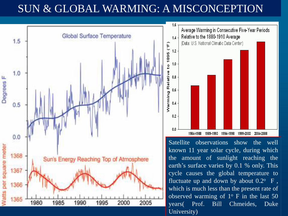
SUN & GLOBAL WARMING: A MISCONCEPTION
Satellite observations show the well
known 11 year solar cycle, during which
the amount of sunlight reaching the
earth’s surface varies by 0.1 % only. This
cycle causes the global temperature to
fluctuate up and down by about 0.2o F ,
which is much less than the present rate of
observed warming of 1o F in the last 50
years( Prof. Bill Chmeides, Duke
University)

TROPOSPHERE vs STRATOSPHERE:
OPPOSITE TEMPERATURE TREND
The Earth’s average surface temperature has increased by 1.4°F (0.8°C) since the
early years of the 20th century. Global average temperature shows rise with the rate
of 0.67 degree centigrade for 100 years between 1891 and 2008. (IPCC,AR5,2013)

RECENT WARMING: OBSERVATIONS AND SIMULATIONS
NATURAL ONLY
NATURAL + MAN-MADE
MAN - MADE ONLY
“Most of the observed warming over the last 50 years is likely to have been due to the increase in greenhouse gas concentration” (IPCC 2013)
Observations
Spread from set of simulations

Anthropogenic climate change is a result of increasing
concentrations of greenhouse gases in the atmosphere:
(a) Carbon-dioxide (CO2)
(b) Methane (CH4)
(c) Nitrous Oxide (N2O)
(d) Chlorofluro carbons
Each of these gases are released in the atmosphere due to
our actions in
Industries
Transportation
Agriculture
Domestic activity and Lifestyle issues
Modern life style is supported by large energy inputs and
material resources producing huge waste
Anthropogenic Climate Change

Atmospheric CO2 measurements
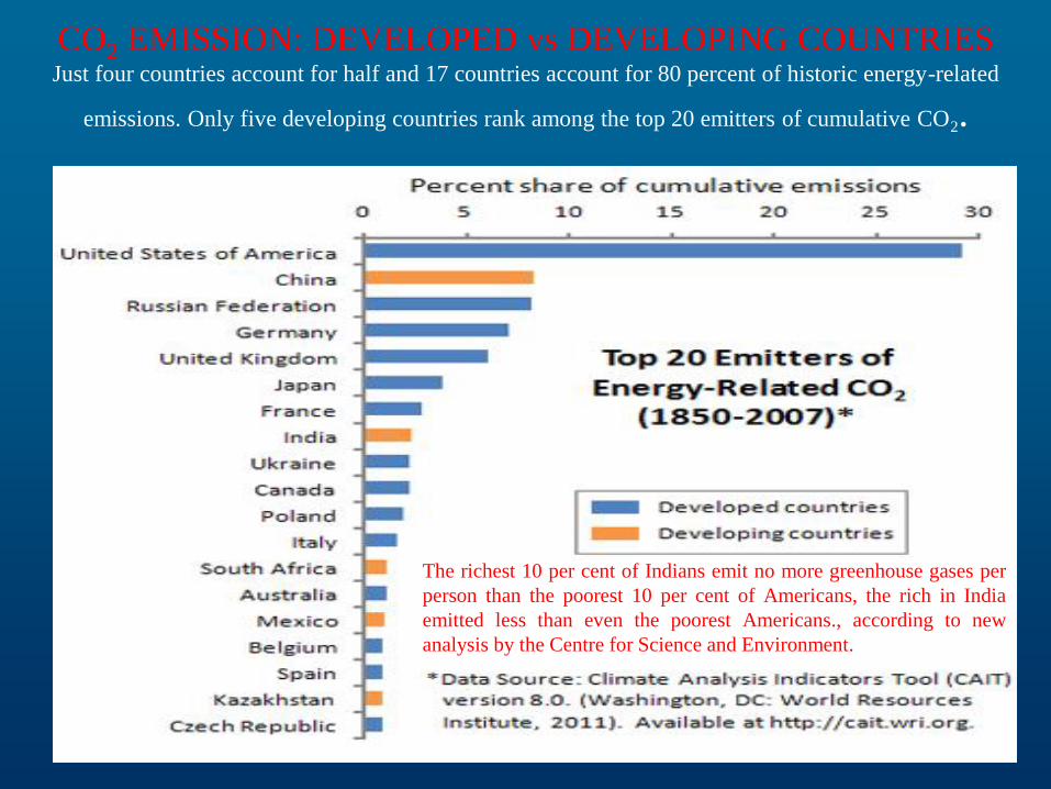
CO2 EMISSION: DEVELOPED vs DEVELOPING COUNTRIES Just four countries account for half and 17 countries account for 80 percent of historic energy-related
emissions. Only five developing countries rank among the top 20 emitters of cumulative CO2.
The richest 10 per cent of Indians emit no more greenhouse gases per
person than the poorest 10 per cent of Americans, the rich in India
emitted less than even the poorest Americans., according to new
analysis by the Centre for Science and Environment.

Increase in GHG are human induced: First, CO2, methane, and nitrous oxide concentrations were stable for thousands of years.
Suddenly, they began to rise like a rocket around 200 years ago, about the time that
humans began to engage in very large-scale agriculture and industry
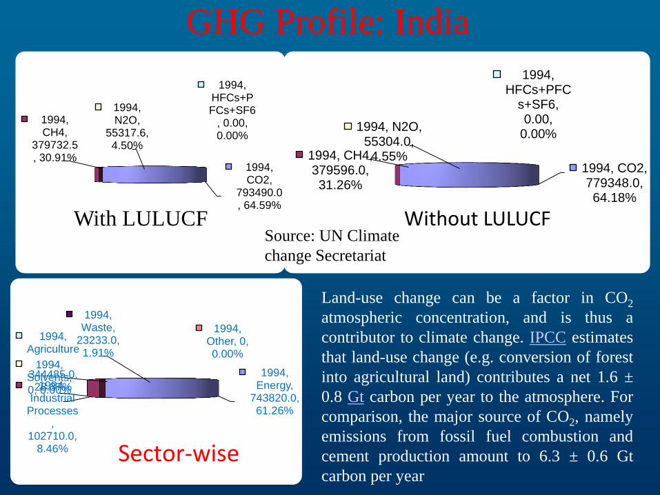
GHG Profile: India
1994, CO2,
793490.0, 64.59%
1994, CH4,
379732.5, 30.91%
1994, N2O,
55317.6, 4.50%
1994, HFCs+PFCs+SF6
, 0.00, 0.00%
With LULUCF
1994, CO2, 779348.0, 64.18%
1994, CH4, 379596.0, 31.26%
1994, N2O, 55304.0, 4.55%
1994, HFCs+PFC
s+SF6, 0.00,
0.00%
Without LULUCF Source: UN Climate
change Secretariat
1994, Energy,
743820.0, 61.26%
1994, Industrial
Processes,
102710.0, 8.46%
1994, Solvents, 0, 0.00%
1994, Agriculture
, 344485.0, 28.37%
1994, Waste,
23233.0, 1.91%
1994, Other, 0, 0.00%
Sector-wise
Land-use change can be a factor in CO2
atmospheric concentration, and is thus a
contributor to climate change. IPCC estimates
that land-use change (e.g. conversion of forest
into agricultural land) contributes a net 1.6 ±
0.8 Gt carbon per year to the atmosphere. For
comparison, the major source of CO2, namely
emissions from fossil fuel combustion and
cement production amount to 6.3 ± 0.6 Gt
carbon per year

Warmest month and warmest year globally Warmest months on record, through 2010
Month Warmest Anomaly
Jan 2007 + 0.81°C + 1.46°F
Feb 1998 + 0.83°C + 1.49°F
Mar 2010 + 0.77°C + 1.39°F
Apr 2010 + 0.73°C + 1.31°F
May 2010 + 0.69°C + 1.24°F
Jun 2005 + 0.66°C + 1.19°F
Jul 1998 + 0.70°C + 1.26°F
Aug 1998 + 0.67°C + 1.21°F
Sep 2005 + 0.66°C + 1.19°F
Oct 2003 + 0.71°C + 1.28°F
Nov 2004 + 0.72°C + 1.30°F
Dec 2006 + 0.73°C + 1.31°F
Rank Year Difference (°F) vs. 20th century
1 2005 1.12
2 2010 1.12
3 1998 1.08
4 2003 1.04
2002 1.04
6 2006 1.01
7 2009 1.01
8 2007 0.99
9 2004 0.97
10 2001 0.94
11 2008 0.86
12 1997 0.86
13 1999 0.76
14 1995 0.74
15 2000 0.70

Urban warming during the last century
Tokyo
New York
Paris
World Ave.
by JMA
Temperature rise during the last century in Japan Not urbanized area 0.2oC Small cities 1.0oC Average of big cities 2.5oC Tokyo 3.0oC
(by JMA and Junsei Kondo)
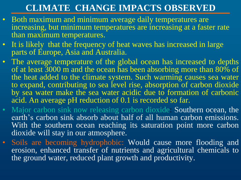
• Both maximum and minimum average daily temperatures are increasing, but minimum temperatures are increasing at a faster rate than maximum temperatures.
• It is likely that the frequency of heat waves has increased in large parts of Europe, Asia and Australia.
• The average temperature of the global ocean has increased to depths of at least 3000 m and the ocean has been absorbing more than 80% of the heat added to the climate system. Such warming causes sea water to expand, contributing to sea level rise, absorption of carbon dioxide by sea water make the sea water acidic due to formation of carbonic acid. An average pH reduction of 0.1 is recorded so far.
• Major carbon sink now releasing carbon dioxide: Southern ocean, the earth’s carbon sink absorb about half of all human carbon emissions. With the southern ocean reaching its saturation point more carbon dioxide will stay in our atmosphere.
• Soils are becoming hydrophobic: Would cause more flooding and erosion, enhanced transfer of nutrients and agricultural chemicals to the ground water, reduced plant growth and productivity.
CLIMATE CHANGE IMPACTS OBSERVED

Observed changes in (a) global
average surface temperature; (b)
global average sea level from tide
gauge and satellite data and (c)
Northern Hemisphere snow cover
for March-April. All differences
are relative to corresponding
averages for the period 1961-
1990. Smoothed curves represent
decadal averaged values while
circles show yearly values. The
shaded areas are the uncertainty
intervals estimated form
comprehensive analysis of known
uncertainties (a and b) and from
the time series (c) (IPCC, 2007)
Global average temperature
shows rise with the rate of 0.67
degree in centigrade for 100
years between 1891 and 2008.
Global average sea level has
risen since 1961 at an average
rate of 1.8mm/yr and since
1993 at 3.1mm/yr, with
contributions from thermal
expansion, melting glaciers
and ice caps, and the polar ice
sheets.

Partial pressure of dissolved CO 2 at the ocean
surface (blue curves) and in situ pH (green
curves), a measure of the acidity of ocean
water. Measurements are from three stations
from the Atlantic (29°10′N, 15°30 ′W – dark
blue/dark green; 31°40′N, 64°10 ′W –
blue/green) and the Pacific Oceans (22°45 ′N,
158°00′W − light blue/light green)
Ocean acidification
is quantified by
decreases in pH .
The pH of ocean
surface water has
decreased by 0.1 since
the beginning of the
industrial era (high
confidence),
corresponding to a
26% increase in
hydrogen ion
concentration.

2002 & 2009 Drought
in India
Rainfall decreased over Western ghat but
increased over central region of India

The unseasonal spell of rain and hail brought a flood of worry for
farmers across North India, having wreaked havoc on Rabi crops
right on the threshold of spring.
Hail outburst
damages
crops, casts
shadow on
Rabi harvest 27 Feb-4, March, 2014

Permanent migration of many
families in Mozambique due to
severe and frequent floods while
the droughts have severely affected
food production, Situation is
equally bad in Bangladesh
CLIMATE CHANGE INDUCED MIGRATION (Mozambique is simultaneously hit by drought and flood in many years)

CLIMATE CHANGE INDUCED MIGRATION
(Mekong Delta in Vietnam is in Peril)
Mekong Delta, the
second largest rice
producer in the world
is in peril because of
severe and frequent
flooding. The region is
highly vulnerable to
sea level rise. 1m rise
would displace 7
million people.
LIVING WITH
FLOODS 1-2m rise in sea
level and
associated coastal
flooding would
displace about
80% of Vietnam
population by
2020

ODISHA is Vulnerable to
Tropical Cyclone
Heatwave Drought
Flood
ODISHA: A State frequently prone to natural disasters
Cyclonic Storms (1891-2007)
Depression and Deep
Depression: 280
Cyclonic storms: 72
Severe Cyclonic Storms,
Very Severe Cyclonic Storms/
Super cyclone: 20
Drought
(1975-1996):23
Floods/Heavy rains
(1975-1996): 88
Heat wave
(1975-1996): 13
Thunderstorms
Tornado (1975-1996): 54
Hail Storm (1975-1996): 55
Gale (1975-1996): 24
Squall (1975-1996): 15
Coastal Erosion

CLIMATOLOGY OF TROPICAL CYCLONES ALONG THE ODISHA COAST
Districts Coastline
(in km)
D CS SCS
Ganjam 63.25 22 6 5
Puri 138 56 17 2
Jagatsinghpur 61.38 33 12 3
Kendrapara 79.43 41 7 4
Bhadrak 49.36 27 7 2
Balasore 88.64 101 23 4
Total 480 280 72 20
Number of D/CS/SCS crossing the six coastal districts of Odisha (1891-2007)
CS (72)
1891-2007
SCS (20)
1891-2007
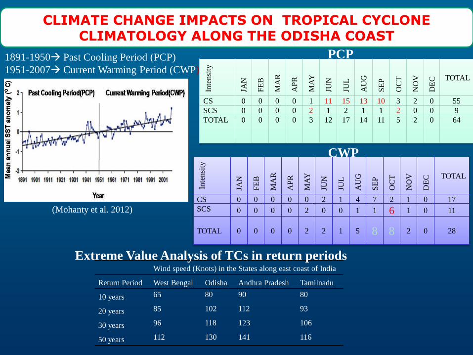
CLIMATE CHANGE IMPACTS ON TROPICAL CYCLONE CLIMATOLOGY ALONG THE ODISHA COAST
1891-1950 Past Cooling Period (PCP)
1951-2007 Current Warming Period (CWP)
(Mohanty et al. 2012) In
tensi
ty
JAN
FE
B
MA
R
AP
R
MA
Y
JUN
JUL
AU
G
SE
P
OC
T
NO
V
DE
C
TOTAL
CS 0 0 0 0 1 11 15 13 10 3 2 0 55
SCS 0 0 0 0 2 1 2 1 1 2 0 0 9
TOTAL 0 0 0 0 3 12 17 14 11 5 2 0 64
Inte
nsi
ty
JAN
FE
B
MA
R
AP
R
MA
Y
JUN
JUL
AU
G
SE
P
OC
T
NO
V
DE
C
TOTAL
CS 0 0 0 0 0 2 1 4 7 2 1 0 17
SCS 0 0 0 0 2 0 0 1 1 6 1 0 11
TOTAL 0 0 0 0 2 2 1 5 8 8 2 0 28
PCP
CWP
Wind speed (Knots) in the States along east coast of India
Return Period West Bengal Odisha Andhra Pradesh Tamilnadu
10 years 65 80 90 80
20 years 85 102 112 93
30 years 96 118 123 106
50 years 112 130 141 116
Extreme Value Analysis of TCs in return periods
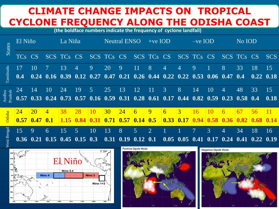
CLIMATE CHANGE IMPACTS ON TROPICAL CYCLONE FREQUENCY ALONG THE ODISHA COAST
Sta
tes El Niño La Niña Neutral ENSO +ve IOD –ve IOD No IOD
TCs CS SCS TCs CS SCS TCs CS SCS TCs CS SCS TCs CS SCS TCs CS SCS
Tam
ilnad
u
17
0.4
10
0.24
7
0.16
13
0.39
4
0.12
9
0.27
20
0.47
9
0.21
11
0.26
8
0.44
4
0.22
4
0.22
9
0.53
1
0.06
8
0.47
33
0.4
18
0.22
15
0.18
Andhra
Pra
des
h 24
0.57
14
0.33
10
0.24
24
0.73
19
0.57
5
0.16
25
0.59
13
0.31
12
0.28
11
0.61
3
0.17
8
0.44
14
0.82
10
0.59
4
0.23
48
0.58
33
0.4
15
0.18
Odis
ha 24
0.57
20
0.47
4
0.1
38
1.15
28
0.84
10
0.31
30
0.71
24
0.57
6
0.14
9
0.5
6
0.33
3
0.17
16
0.94
10
0.58
6
0.36
67
0.82
56
0.68
11
0.14
Wes
t B
engal
15
0.36
9
0.21
6
0.15
15
0.45
5
0.15
10
0.3
13
0.31
8
0.19
5
0.12
2
0.1
1
0.05
1
0.05
7
0.41
3
0.17
4
0.24
34
0.41
18
0.22
16
0.19
(the boldface numbers indicate the frequency of cyclone landfall)
El Niño

Coefficient of variation of rainfall
Annual 19-29%
Pre monsoon 40-80%
SW monsoon 17-30%
Post monsoon 58-130%
Winter 90-170%
Contribution of the seasonal rainfall to
the total annual rainfall
SW Monsoon (JJAS) 79%
Winter (DJF) 3%
Pre-monsoon (MAM) 8%
Post-monsoon (ON) 10%
ODISHA RAINFALL(Mean annual rainfall: 145 cm)

Drought & Excessive rainfall Conditions
Moderate drought: If rainfall deficit is between 25-50% of the normal
Severe drought: If the rainfall deficit is more than 50% of the normal
Districts Number of
drought
year(1901-
1990)
Frequency of
drought(%)
Districts Number of
drought
year(1901-
1990)
Frequency of
drought(%)
Districts Number of
drought
year(1901-
1990)
Frequency of
drought(%)
Angul 10 12 Ganjam 7 8 Malkanagiri 6 13
Balasore 7 9 Jagatsingha
pur 1 2 Mayurbhanj
a 2 3
Baragarh 8 11 Jajpur 3 5 Nayagarh 3 5
Boudh 4 9 Jharsuguda 4 6 Nuapada 7 11
Bhadrak 3 3 Kandhamal
a 5 6 Nabarangap
ur 2 5
Bolangir 2 3 Kalahandi 7 12 Puri 4 5
Cuttack 3 3 Kendrapara 6 10 Rayagada 4 6
Deogarh 5 11 Keonjhar 9 12 Sambalpur 6 7
Dhenkanal 2 3 Khurda 4 5 Sonepur 12 18
Gajapati 2 3 Koraput 5 7 Sundargarh 5 8

Excessive Rainfall (Annual rainfall
of 125% or more of the normal) Districts Average annual
(Normal) rainfall
(mm)
Successive Years of excessive Rainfall Heaviest rainfall
record in 24 hours
(year within bracket)
Angul 1401.9 1960-61 339.0 (1991)
Balasore 1592.0 1940-41,1960-61 479.3 (1943)
Baragarh 1367.3 1936-37,1963-64 368.3 (1939)
Boudh 1623.1 1939-40,1954-55-56 395.0 (1936)
Bhadrak 1427.9 1955-56 514.6 (1879)
Bolangir 1289.8 1917-18-19,1985-86 325.8 (1958)
Cuttack 1424.3 1955-56 416.8 (1934)
Deogarh 1582.5 - 330.2 (1943)
Dhankanal 1428.8 1956-57 305.0 (1991)
Gajapati 1403.3 - 319.2 (1990)
Ganjam 1276.2 - 445.0 (1990)
Jagatsinghpur 1514.6 1916-17,1936-37 498.6 (1889)
Jajpur 1559.9 1985-86 350.0 (1992)
Jarsuguda 1362.8 1933-34,1936-37,1960-61 350.0 (1925)

Excessive Rainfall (Annual rainfall
of 125% or more of the normal) Districts Average annual
(Normal)
rainfall (mm)
Successive Years of excessive Rainfall Heaviest rainfall
record in 24 hours
Kalahandi 1330.5 1910-11,1955-56-57 344.1 (1967)
Kandhamala 1427.9 1925-26 331.0 (1991)
Kendrapara 1556.0 - 401.8 (1925)
Keonjhar 1487.7 - 343.4 (1941)
Khurda 1408.4 1973-74-75 325.0 (1974)
Koraput 1567.2 - 546.1 (1931)
Malkanagiri 1667.6 - 306.3 (1907)
Mayurbhanja 1630.6 1940-41, 1977-78 467.4 (1973)
Nayagarh 1354.3 - 273.1 (1945)
Nuapara 1286.4 1919-20 279.4 (1917)
Nabarangapur 1569.5 - 350.0 (1973)
Puri 1408.8 1946-47 480.1 (1862)
Rayagada 1285.9 1916-17 355.6 (1890)
Sambalapur 1495.7 1907-08,1919-20,1960-61 581.9 (1982)
Sonepur 1418.5 1917-18,1932-33,1985-86 365.5 (1918)
Sundargarh 1422.4 1919-20,1961-62 333.5 (1920)

Origin of Heat Wave
• Heat wave due to advection
– Advection of heat from northwest India due to stronger westerly to northwesterly wind.
– Large amplitude anticyclonic flow (thickness of atmosphere above normal) and dry adiabatic lapse rate helps in thermal advection.
• Heat wave in situ
– Weak/ delayed onset of sea breeze.
– Less cloudiness and less relative humidity are favourable for heat wave.

Mean pressure & Prevailing Wind - MAY

UPPER WINDS (0.5 km) – MAY

UPPER WINDS (1.0 km) – MAY

Urban Heat Island

Causes of Urban heat Island Sl.
No.
Effect Mechanism
1 Increased counter radiation Absorption of LWR up and
emission by pollutants
2 Decreased net long-wave
radiation
Increase in atmospheric
pollutant levels
3 Greater day time heat
storage
Thermal properties of
construction materials
4 Decreased evaporation Removal of vegetation and
surface waterprofing
5 Decreased sensible heat
loss
Reduced wind speed

GOPALPUR BALASORE SAMBALPUR ANGUL
CUTTACK CHANDABALI PURI BARIPADA
HIRAKUD TITLAGARH KEONJHARGARH
JHARSUGUDA BOLANGIR BHAWANIPATNA PARADEEP
BHUBANESWAR KORAPUT
JHARSUGUDA
PE
P
Water Deficit
Water Recharge
Water Surplus
Water Balance along major places of Odisha
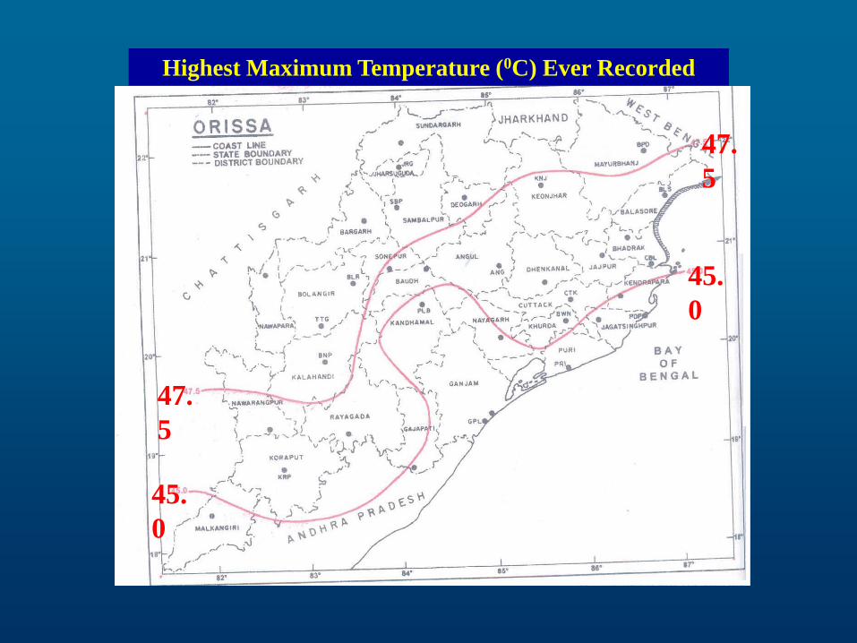
Highest Maximum Temperature (0C) Ever Recorded
47.
5
47.
5
45.
0
45.
0

Mean Maximum Temperature (0C) - MAY
37.
5
37.
5
35.
0
32.
5
32.
5
35.
0
37.
5
42.
5
40.
0

Critical temperatures (0 C) for malaria transmissions
Mean Annual Maximum Temperature (0C) Mean Annual Minimum Temperature (0C)

I M D Definition of Heat Wave Places where the normal maximum temperature is more than 40 0 C:
Day Temperature > 3 – 4 0C above normal: Heat Wave
Day Temperature > 5 0C above normal: Sever Heat Wave
Places where the normal maximum temperature is less than 40 0 C:
Day Temperature > 5 – 6 0C above normal: Mod. Heat Wave
Day Temperature > 6 0C above normal: Sever Heat Wave
MAX TEMP_JHARSUGUDA
2829
303132
333435
363738
3940
414243
444546
4748
1 7 13 19 25 31 37 43 49 55 61 67 73 79 85 91 97 103 109 115 121
Heat Index
Too Hot
Thermo-Hygrometric Index THI = Tmax – [(0.55 – 0.0055 RH%)(Tmax –14.5)] 0C
Mortality and Morbidity depends on Complex thermo-hygrometric Index (Tseletidaki et al, 1995)
THI > 28.5 is usually associated with discomfort.
Apparent Temperature The ambient temperature adjusted for variations in vapour pressure above or below some base value
and is expressed as a function of Temperature, humidity and wind speed )
AT = -2.653+(0.994 Ta )+ (0.0153 Td)2
16- 25 0C – Mild conditions :
Clothing thickness ( 7.64-0.20 mm)
Skin thermal resistance ( 0.0387 m2 K w -1)
Skin Moisture resistance ( 0.0521 m2 K w -1) 25- 50 0C – Severe conditions :
Clothing thickness ( 0.00 mm)
Skin thermal resistance ( 0.0377-0.0229 m2 K w -1)
Skin Moisture resistance ( 0.0446-0.0037 m2 K w -1)
Heat Index: heat-humidity combination
make the condition dangerous
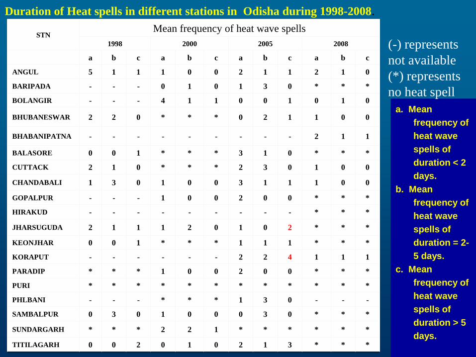
STN Mean frequency of heat wave spells
1998 2000 2005 2008
a b c a b c a b c a b c
ANGUL 5 1 1 1 0 0 2 1 1 2 1 0
BARIPADA - - - 0 1 0 1 3 0 * * *
BOLANGIR - - - 4 1 1 0 0 1 0 1 0
BHUBANESWAR 2 2 0 * * * 0 2 1 1 0 0
BHABANIPATNA - - - - - - - - - 2 1 1
BALASORE 0 0 1 * * * 3 1 0 * * *
CUTTACK 2 1 0 * * * 2 3 0 1 0 0
CHANDABALI 1 3 0 1 0 0 3 1 1 1 0 0
GOPALPUR - - - 1 0 0 2 0 0 * * *
HIRAKUD - - - - - - - - - * * *
JHARSUGUDA 2 1 1 1 2 0 1 0 2 * * *
KEONJHAR 0 0 1 * * * 1 1 1 * * *
KORAPUT - - - - - - 2 2 4 1 1 1
PARADIP * * * 1 0 0 2 0 0 * * *
PURI * * * * * * * * * * * *
PHLBANI - - - * * * 1 3 0 - - -
SAMBALPUR 0 3 0 1 0 0 0 3 0 * * *
SUNDARGARH * * * 2 2 1 * * * * * *
TITILAGARH 0 0 2 0 1 0 2 1 3 * * *
a. Mean
frequency of
heat wave
spells of
duration < 2
days.
b. Mean
frequency of
heat wave
spells of
duration = 2-
5 days.
c. Mean
frequency of
heat wave
spells of
duration > 5
days.
(-) represents
not available
(*) represents
no heat spell
Duration of Heat spells in different stations in Odisha during 1998-2008.

2013201220112010200920082007200620052004200320022001200019991998
District wise mortality during 1998-2013

Different Temperature Zones in Odisha and their temperature ranges
Coastal Odisha: >=350 C < 390C (Gopalpur, Paradeep, Puri) North-Central Odisha: >=420C < 44.50C (Balasore, Cuttack, Baripada, Phulabani, Keonjhar, Chandbali, Bhubaneswar) Western Odisha: >=44.50C <= 480C (Titilagarh, Bhawanipatna, Jharsuguda, Bolangir, Anugul, Sambalpur, Sundergarh, Hirakuda) Southern Odisha: >390C <=400C (Koraput)
Physiographic features of Odisha

Year/Sta
tion
Coastal Stations North Central station Western station Southern stations
Number
of
mortality
Number
of heat
spells
Number
of
mortality
Number
of heat
spells
Number of
mortality
Number of
heat spells
Number of
mortality
Number of
heat spells
1998 138 3 736 14 446 17 0 NA
1999 7 1 38 23 5 30 0 NA
2000 0 2 9 2 19 12 0 NA
2001 2 3 6 2 6 7 0 NA
2002 11 7 7 7 7 16 0 NA
2003 9 1 8 14 14 16 0 NA
2004 9 4 11 20 5 14 0 4
2005 41 4 70 28 50 17 0 8
2006 4 3 5 8 12 8 0 2
2007 9 2 11 6 7 13 1 2
2008 14 0 20 3 13 8 0 3
Total 244 30 921 127 584 158 1 19
Heat spell and mortality in different temperature zones of Odisha

y = 0.0692x + 31.812 R² = 0.1952
GPL-May(Max. Temp.)
y = 0.0093x + 33.327 R² = 0.0044
PDP-May(Max. Temp.)
y = 0.0948x + 30.194 R² = 0.0452
PURI-May(Max. Temp.)
y = -0.0464x + 26.49 R² = 0.0595
GPL-May(Min. Temp.)
y = -0.056x + 26.3 R² = 0.0597
PDP-May(Min. Temp.)
y = -0.0531x + 26.932 R² = 0.0198
PURI-May(Min. Temp.)
PU
RI
PA
RA
DIP
G
OPA
LP
UR
Comparison of Max. and Min. Temperature trends along Coastal Odisha during May

y = 0.0646x + 36.682 R² = 0.1462
BSR-May(Max. Temp.)
y = 0.0625x + 38.136 R² = 0.0972
PLB-May(Max. Temp.)
y = 0.0576x + 37.6 R² = 0.0516
BPD-May(Max. Temp.)
y = -0.0724x + 26.747 R² = 0.1599
BPD-May(Min. Temp.)
y = -0.068x + 27.129 R² = 0.2119
BSR-May(Min. Temp.)
y = -0.163x + 24.839 R² = 0.2819
PLB-May(Min. Temp.)
PH
UL
BA
NI
BH
UB
AN
ES
WA
R
BA
RIP
AD
A
Comparison of Max. and Min. Temperature trends along North Central Odisha during May

y = 0.1113x + 38.581 R² = 0.1102
SMB-May(Max. Temp.)
y = 0.1007x + 41.646 R² = 0.2656
TTG-May(Max. Temp.)
y = 0.1278x + 38.658 R² = 0.388
ANG-May(Max. Temp.)
y = -0.1047x + 26.422 R² = 0.241
ANG-May(Min. Temp.)
y = -0.0959x + 27.59 R² = 0.2202
SMB-May(Min. Temp.)
y = -0.0656x + 27.564 R² = 0.1144
TTG-May(Min. Temp.)
TIT
ILA
GA
RH
S
AM
BA
LP
UR
A
NG
UL
Comparison of Max. and Min. Temperature trends along Western Odisha during May
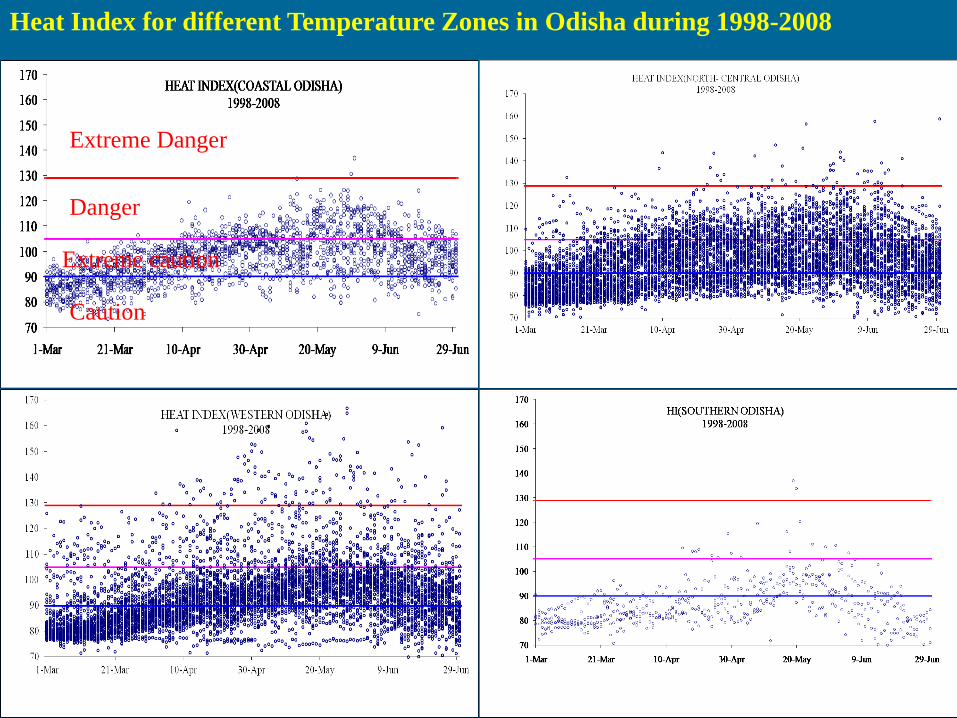
Heat Index for different Temperature Zones in Odisha during 1998-2008
Extreme Danger
Danger
Extreme caution
Caution

Thermo Hygrometric Index for different Temperature Zones in Odisha during 1998-2008
Discomfort
Comfort
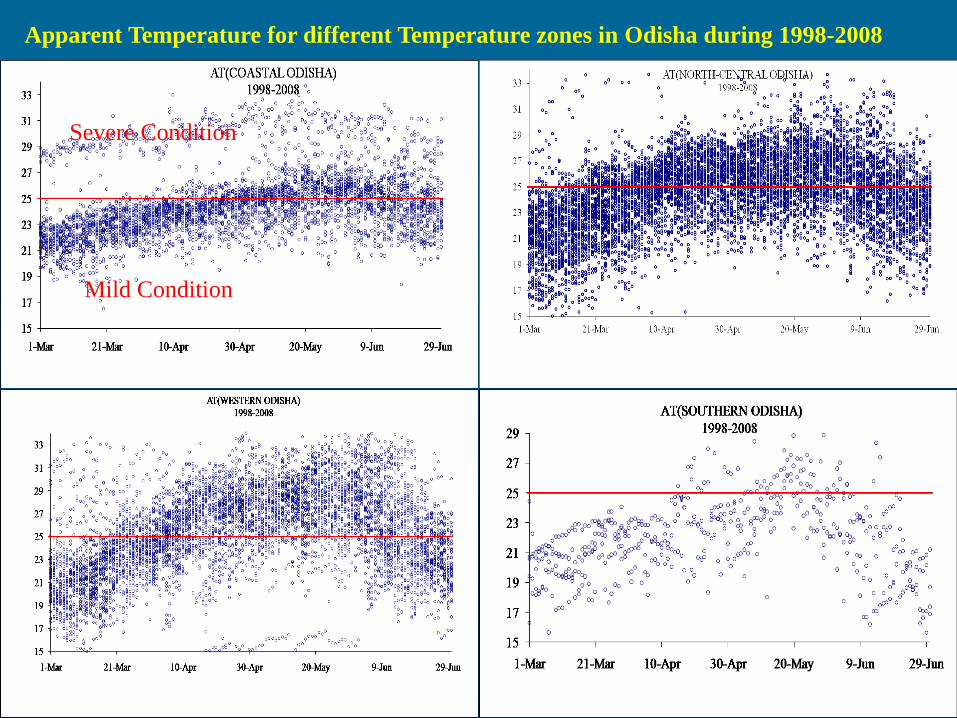
Apparent Temperature for different Temperature zones in Odisha during 1998-2008
Severe Condition
Mild Condition
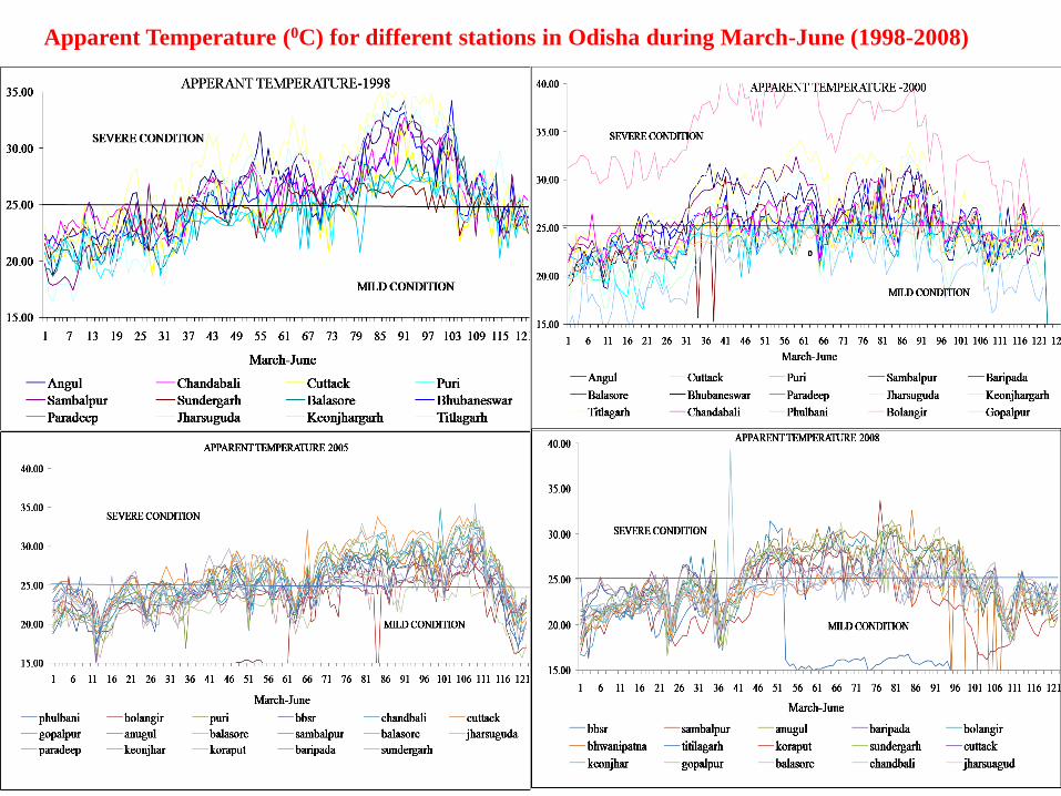
Apparent Temperature (0C) for different stations in Odisha during March-June (1998-2008)

TP-MWD_JJAS
Above 24
18 - 24
12 - 18
6 - 12
Below 6
NCalm
3.72 %
10 %
HM0-MWD_JJAS
Above 2
1.5 - 2
1 - 1.5
0.5 - 1
0.3 - 0.5
Below 0.3
N
Calm0.00 %
10 %
HM0-MWD-ON
Above 2
1.5 - 2
1 - 1.5
0.5 - 1
0.3 - 0.5
Below 0.3
NCalm
0.00 %
10 %
TP-MWD_ON
Above 24
18 - 24
12 - 18
6 - 12
Below 6
NCalm
1.67 %
10 %
HM0-MWD_DJF
Above 2
1.5 - 2
1 - 1.5
0.5 - 1
0.3 - 0.5
Below 0.3
NCalm
0.74 %
10 %
TP-MWD_DJF
Above 24
18 - 24
12 - 18
6 - 12
Below 6
NCalm
5.17 %
10 %
HM0-MWD_MAM
Above 2
1.5 - 2
1 - 1.5
0.5 - 1
0.3 - 0.5
Below 0.3
N
Calm0.00 %
10 %
TP-MWD_MAM
Above 24
18 - 24
12 - 18
6 - 12
Below 6
N
Calm24.84 %
10 %
June-July-Aug.-Sept.
High Energy
Oct.- Nov.
Low. Energy
Dec.- Jan.- Feb.
Very low Energy
Mar.- Apr.-May
Moderate Energy
Significant Wave Height (m)
Peak Wave Period (sec)
Wave Rider Buoy data collected during May 2008-June 2009 off Gopalpur

August_2010
August_2014 August_2013
August_2008
Erosion at Gopalpur tourist beach
July_2014
August_2009
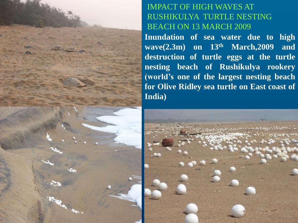
Inundation of sea water due to high
wave(2.3m) on 13th March,2009 and
destruction of turtle eggs at the turtle
nesting beach of Rushikulya rookery
(world’s one of the largest nesting beach
for Olive Ridley sea turtle on East coast of
India)
IMPACT OF HIGH WAVES AT
RUSHIKULYA TURTLE NESTING
BEACH ON 13 MARCH 2009

Prediction of tsunami inundation at N.Andaman using 2004 Sumatra source parameters
Date of Occurrence : 26-Dec-2004
Tsunamigenic source : Sumatra
Location : 92.5 E, 12.1 N
EQ magnitude : 9.3 Mw
Slip magnitude : 15 m
Fault length : 500 km
Fault width : 150 km
Strike : 345 deg.
Dip : 15 deg.
Rake : 90 deg.
Depth : 20 km
Extent of Inundation without tide
Extent of Inundation with tide
415m
300m
370m
320m
Puri
Orissa coast close to N.Andaman Tsunami source. 1941 Tsunami had no impacts
if tsunami occurs at N.Andaman at same magnitude as 2004

Gopalpur
Gopalpur port
Haripur
Creek
North Andman Source Sumatra Parameters (Worst scenario)
Sumatra : 26 December 2004 earthquake case
North Andaman: 26 June 1941 earthquake case
Bathymetry : Cmap+Gebco
Elevation : RTK + SRTM + Gebco
Inundation at Gopalpur, Orissa
Maximum inundation at Haripur creek for worst case : 0.6 km
maximum Run up: 5.0 m

CLIMATE CHANGE IS HAPPENING…….
…..AND ITS EFFECTS ARE LIKELY TO BE VERY PROFOUND AND WHAT WILL BE FUTURE CLIMATE AND ITS IMPACT

Climate changes over the next few decades are predicted to be much larger than we have seen so far…
The war against Global Warming could be worse than that
against Global Terrorism

THE DAY AFTER TOMORROW
We must avoid such a tomorrow. Therefore, we should understand the climate change,
educate key policy-makers and the public about the causes and potential consequences
of climate change and to assist the domestic and international communities in
developing practical and effective solutions to this important environmental challenge.

CLIMATE SWINGS : Medieval warm
to little ice age, present and future
Implications: Millions of people near equator would experience dry condition, Crops like coffee,
banana and tropical biodiversity would wither in places such as Ecuador, Colombia, northern Indonesia and
Thailand. Serious drought in southwestern US. Locations near the band would experience high temperature
and heavy rain. No idea yet on the frequency and intensity of hurricanes and monsoons
Meridional swing of
Intertropical
convergence
Zone(ITCZ)
southerly position-
cool climate
Northerly position-
warm and wet climate

Baseline
Scenario (1961–1990)
A2 scenario (2071–2100
The composite tracks of the cyclones for the baseline
and A2 Scenarios do not show any significant difference
The frequency of cyclones during the late monsoon
season during the future (2071–2100) scenario is found to
be much higher than that during the baseline scenario.
Maximum wind speed indicates higher number of intense
cyclones in the A2 scenario than that in the baseline
scenario.

Flood/Drought conditions in different river
basins of India under climate change scenario
Mahanadi and
Bramhani River basins
are expected to receive
comparatively higher
level of precipitation in
future and a
corresponding increase
in evapotranspiration
and water yield is also
predicted.
Increase in flood peak
shall be detrimental to
both life and property
in these river basins

ANNUAL NUMBER OF PEOPLE FLOODED
Change from the present day to the 2080s (unmitigated emissions)
In many parts of the world, climate change may be disastrous…….

Annual Temperature Scenarios for States of India, based on PRECIS, for 2071-2100
Source: IITM,Pune
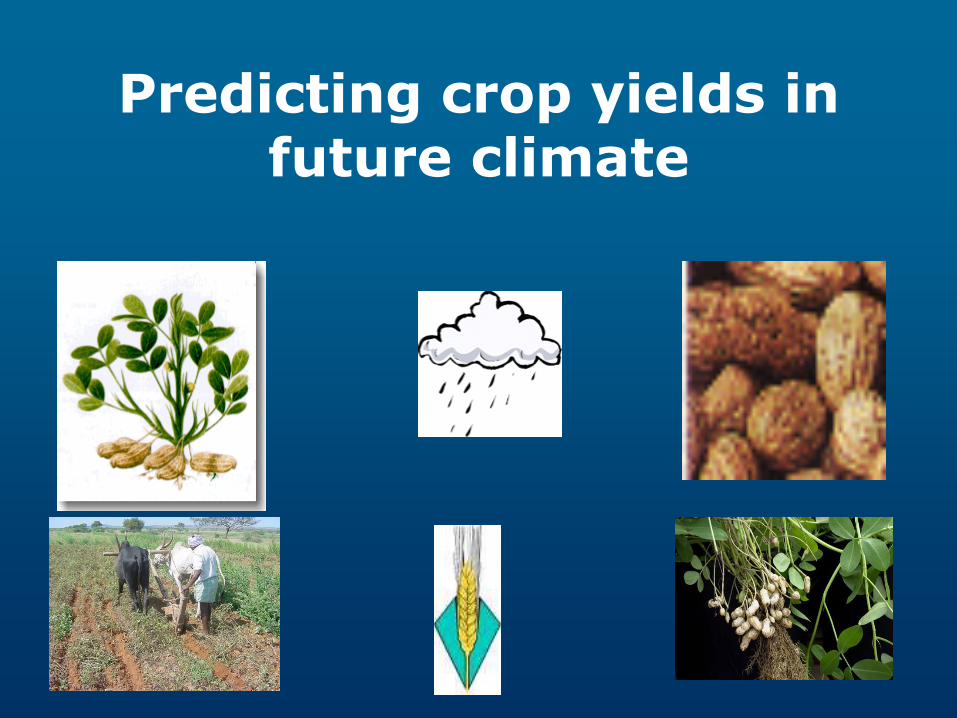
Predicting crop yields in future climate

LINKING CROP WITH CLIMATE
CLIMATE CHANGE:
•Increase in air Temperature
•Increase in CO2 content
•More evaporation and less
precipitation
•Lowering of the water table
CROP RESPONSE:
•Accelerated crop development
•Reduction in the length of the
effective growing season in the
tropics
•Increase in the length of the
effective growing season in areas
where agricultural potential is
currently limited by cold
temperature stress
•CO2-induced increases in crop
yields are much more probable in
warm than in cool environments
•Increase in water stress, both by
the root system and leaf
•What will happen to the over all
productivity?
Autocatalytic component to global warming:
Photosynthesis and respiration of plants and
microbes increase with temperature, especially in
temperate latitudes. As respiration increases more
with increased temperature than does
photosynthesis, global warming is likely to increase
the flux of carbon dioxide to the atmosphere which
would constitute a positive feedback to global
warming.

TE=ctl TE=1.5*ctl
TE=2.0*ctl TE=2.5*ctl
Effect of CO2 fertilisation on groundnut crop yields in future climates: 2080-2100
10-40% loss in crop production in India by 2080-2100 due to global
warming despite beneficial aspect of increased CO2
Source:
Walker
Institute
University
of Reading,
UK

Percentage variation in rainfed and irrigated rice
and maize along coastal zone of India during
2020-2050
Yield of maize
and sorghum,
having c4
photosynthetic
system, is likely to
reduce by 50% due
to climate change
Rice yields
decrease 9% for
each 1°C increase
in seasonal average
temperature

CLIMATE CHANGE AND AGRICULTURE IN ODISHA
• Odisha coast is projected to have less increase in
temperature i.e. 1o by 2020-2050.Irrigated rice yields are
projected to increase by <5% in Odisha by 2020-2050
due to lesser increase in temperature.
• Rain fed rice yields are projected to increase by 15%
along east coast and reduce by 20% along west coast.
• Irrigated maize crops are likely to have yield loss between
15-50% while rain fed maize shall have yield loss by 35%
• Kharif seasonal rainfall is projected to increase by 10%.
• Marginal increase in rainfall may not hamper the
sunshine period in this region, providing ample scope for
the plants to carry on photosynthetic process, thus
benefiting the rice yield in elevated CO2 conditions.

What needs to be done? • The NAPCC, India aims to promote climate adaptation in agriculture through
the development of climate-resilient crops, expansion of weather insurance
mechanisms, and agricultural practices. As one of the eight missions under
NAPCC
To rebuild food system, development of climate resilient crops
and adaptation mechanisms should be aggressively followed
Use of sea water, a social resource, should be encouraged for
extensive agro and aqua farming

Quickest way to combat
global warming is to
reduce black carbon

Challenges in building Climate
Change Resilience: Climate science and climate policy inhabit parallel words(Nature, 15 Dec,
2011) .
Climate negotiations: a major exercise in diplomacy
Adaptation to climate change is a challenge for all countries. From a global perspective, the adaptation challenge is probably greatest for developing countries. They are generally more vulnerable to climate change because their economies are more dependent on climate-sensitive sectors, such as agriculture, fishing, and tourism. With lower per capita incomes, weaker institutions, and limited access to technology, developing countries have less adaptive capacity.
Food security for the developing countries is a serious challenge which can be addressed through convergence of climate science and policy involving both developed and developing nations.
Strengthen international institutions and policy to protect the rights of those displaced by climate change.
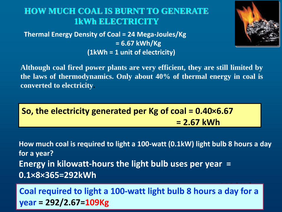
Although coal fired power plants are very efficient, they are still limited by
the laws of thermodynamics. Only about 40% of thermal energy in coal is
converted to electricity.
Thermal Energy Density of Coal = 24 Mega-Joules/Kg = 6.67 kWh/Kg (1kWh = 1 unit of electricity)
How much coal is required to light a 100-watt (0.1kW) light bulb 8 hours a day for a year?
Energy in kilowatt-hours the light bulb uses per year = 0.1×8×365=292kWh = 292 kWh Coal required to produce 292 kWh = 292/2.67 = 109Kg
HOW MUCH COAL IS BURNT TO GENERATE
1kWh ELECTRICITY
So, the electricity generated per Kg of coal = 0.40×6.67 = 2.67 kWh
Coal required to light a 100-watt light bulb 8 hours a day for a year = 292/2.67=109Kg

• Atomic Weight of C = 12, Atomic Weight of O = 16
• Carbon combines with oxygen in the atmosphere during combustion producing CO2 with molecular weight of 44 (12+16×2)
• Assume that coal has 50% carbon in it (by mass), 1 Kg of coal contains at least 0.5 Kg carbon
• CO2 produced from burning 1 Kg of coal (0.5 Kg carbon)
= (44/12) ×0.5
= 1.83 Kg
1 Kg of Coal combustion 1.83 Kg CO2 CO2 produced from burning 109 Kg of coal (0.5 Kg carbon)
= 1.83x109=199.5 kg to light a 100-watt light bulb 8 hours a day for a year
CARBON FOOTPRINT Measure of the impact human activities have on the environment in terms of the
amount of GHG produced, measured in units of CO2. A carbon footprint is often
expressed as tons of CO2 emitted usually on a yearly basis.

Climate Resilient Actions
• INVEST IN DEVELOPING POWER SAVING TECHNOLOGY
RATHER THAN CREATING NEW POWER PLANTS
(Average consumption of electricity per day per household
= 26 kWh, Amount of coal required daily to produce 26 kWh
electricity = 9.7 Kg)
Total CO2 emission per household per day = 17.8 Kg
IMPROVING PUBLIC TRANSPORT SYSTEM is the essential need
, which will reduce air pollution (SO2, NOx, SPM) and greenhouse
gas emission(A bus emits about 700g of CO2 per km compared to
98g/km by a car, a bus can replace 40 cars, which is equivalent to
saving of CO2 emission by about 3.2 Kg/km)
SHIFT FROM COAL BASED ENERGY TO RENEWABLE
ENERGY(solar, tide, wind etc.)
• CLIMATE AUDIT

WHAT YOU/WE CAN/SHOULD DO:
Say NO to Apples from Washington
And YES Apples from
Himachal Pradesh
Dust your Tubelight & Bulbs.
Turn off lights when not
required.
Buy the right wattage for
your needs
Keep Electrical Gadgets in efficient working conditions
Avoid Room-heater through
proper clothing
Plan your building allowing free
airflow and light to cut down use of
fans and electric bulbs
Use Day light hours to cut down
light bills
Reduce garbage in the
neighbourhood
Walking/cycling over short distances
Use public transport
Plant and adopt trees in your areas

We must protect the Earth
Apollo 12’s Classic Earth Rise from Moon
THANK YOU