Policy Research Working Paper 7477

Climate Change Impacts and Mitigation in the Developing World

An Integrated Assessment of the Agriculture and Forestry Sectors

Petr HavlíkHugo Valin

Mykola GustiErwin SchmidDavid LeclèreNicklas ForsellMario Herrero

Nikolay KhabarovAline Mosnier

Matthew CanteleMichael Obersteiner

Development EconomicsClimate Change Cross-Cutting Solutions Area November 2015

Shock Waves: Managing the Impacts of Climate Change on Poverty

Background Paper

WPS7477P

ublic

Dis

clos

ure

Aut

horiz

edP

ublic

Dis

clos

ure

Aut

horiz

edP

ublic

Dis

clos

ure

Aut

horiz

edP

ublic

Dis

clos

ure

Aut

horiz

ed

Produced by the Research Support Team

Abstract

The Policy Research Working Paper Series disseminates the findings of work in progress to encourage the exchange of ideas about development issues. An objective of the series is to get the findings out quickly, even if the presentations are less than fully polished. The papers carry the names of the authors and should be cited accordingly. The findings, interpretations, and conclusions expressed in this paper are entirely those of the authors. They do not necessarily represent the views of the International Bank for Reconstruction and Development/World Bank and its affiliated organizations, or those of the Executive Directors of the World Bank or the governments they represent.

Policy Research Working Paper 7477

This paper was commissioned by the World Bank Group’s Climate Change Cross-Cutting Solutions Area and is a background paper for the World Bank Group’s flagship report: “Shock Waves: Managing the Impacts of Climate Change on Poverty.” It is part of a larger effort by the World Bank to provide open access to its research and make a contribution to development policy discussions around the world. Policy Research Working Papers are also posted on the Web at http://econ.worldbank.org. The authors may be contacted at havlikpt@iiasa.ac.at and valin@iiasa.ac.at.

This paper conducts an integrated assessment of climate change impacts and climate mitigation on agricultural commodity markets and food availability in low- and middle-income countries. The analysis uses the partial equilibrium model GLOBIOM to generate scenarios to 2080. The findings show that climate change effects on the agricultural sector will increase progressively over the century. By 2030, the impact of climate change on food consumption is moderate but already twice as large in a world with high inequalities than in a more equal world. In the long run, impacts could be much stronger, with global average calorie losses of 6 percent by 2050 and 14 percent by 2080. A mitigation policy to stabilize climate below 2°C uniformly applied to all regions as a carbon tax would

also result in a 6 percent reduction in food availability by 2050 and 12 percent reduction by 2080 compared to the reference scenario. To avoid more severe impacts of climate change mitigation on development than climate change itself, revenue from carbon pricing policies will need to be redistributed appropriately. Overall, the projected effects of climate change and mitigation on agricultural markets raise important issues for food security in the long run, but remain more limited in the medium term horizon of 2030. Thus, there are opportunities for low- and mid-dle-income countries to pursue immediate development needs and thus prepare for later periods when adapta-tion needs and mitigation efforts will become the greatest.

Climate Change Impacts and Mitigation in the Developing World: An 

Integrated Assessment of the Agriculture and Forestry Sectors* 

Petr Havlíka, Hugo Valina, Mykola Gustia, Erwin Schmidb, David Leclèrea, Nicklas Forsella, Mario 

Herreroc, Nikolay Khabarova, Aline Mosniera, Matthew Cantelea, Michael Obersteinera 

Keywords: food security, climate change, land use change, bioenergy, poverty 

JEL: Q10, Q23, Q54, Q56 

* Corresponding authors: Petr Havlík (havlikpt@iiasa.ac.at) and Hugo Valin (valin@iiasa.ac.at). Analysis contributing to this study was partly conducted in partnership with the CGIAR Research Program on Climate Change, Agriculture and Food Security (CCAFS).The results and views expressed in this document are the sole personal responsibility of the authors and do not reflect those of their institutions of affiliation. Any errors or omissions remain the responsibility of the authors.

a International Institute for Applied Systems Analysis (IIASA), A‐2361, Laxenburg, Austria. b Institute for Sustainable Economic Development, University of Natural Resources and Life Sciences, A‐1200 Vienna, Austria c Commonwealth Scientific and Industrial Research Organisation, Brisbane, QLD, 4067, Australia 

2  

Summary of main findings 

We generate scenarios  through 2080 with  the partial equilibrium model GLOBIOM and  look at  the 

impacts of climate change and climate mitigation policies at different time horizons, with a focus on 

the medium term 2030 as these impacts could hamper immediate development goals. The main results 

are: 

On the climate change impact and adaptation side 

In the most optimistic scenario, average crop yield across climate models is found to decrease 

by 2% globally by 2030, even when  the positive effects of elevated CO2 concentration are 

accounted for. Without CO2 effects, these impacts could be as severe as ‐10% in 2030 already.  

Climate  change will  hit  regions  unevenly  but  least  advanced  countries will  be  particularly 

affected. The most severely exposed regions by changes in crop yield are South Asia, Eastern 

Asia and Pacific, and Latin America, where agriculture will need to adapt drastically. Impacts 

in Sub‐Saharan Africa and North Africa Middle‐East should be partly attenuated by CO2 effects, 

but will also become severe if this effect does not materialize. 

The societal impacts of these changes will depend on the adaptation capacity of the different 

regions. Various adaptation channels can be used to mitigate the impact of climate change on 

food supply: i) change in crop management at field level (input level, irrigation), ii) change in 

the choice of crops cultivated,  iii)  reallocation of production within  regions,  iv)  increase  in 

cultivated areas, v) international trade adjustments. 

The possibilities to use these mechanisms will be  influenced by the  level of development of 

the agricultural sector as well as the investment capacity and the institutional environment, 

locally and globally. We  look at  two different contexts of  these dimensions across  the  two 

Shared Socio‐Economic Pathways SSP4  (low adaptation capacity and dysfunctional markets 

and institutions for least advanced countries) and SSP5 (high adaptation capacity, integrated 

markets and an enabling institutional environment in least advanced countries).  

At the global level, and for the two background socioeconomic scenarios, no significant price 

variation  is observed  in  the  long  run  if climate change  is contained at 2 degrees. On some 

specific markets, effects  could however be  visible  as  soon  as 2030:  +15/27%  for  sorghum 

(with/without CO2 effects), +7/25% for millet, +4/15% for soya, +2/11% for corn, +0/7% for 

cassava. 

The impact on food supply remains very limited by 2030. On average across climate scenarios 

and SSPs, global consumption decreases by 0.6% with CO2 effects and 1.9% without CO2 effects 

compared  to a  situation without  climate  change. These  impacts become more  severe and 

more  largely  influenced  by  the  baseline  assumption  over  time.  Impacts  reach  ‐2.0/‐4.3% 

(with/without CO2 effects) by 2080 under a macroeconomic scenario favorable to adaptation 

(SSP5) and up to ‐4.4/‐8.7% under poor adaptation capacity (SSP4). 

South Asia and Sub‐Saharan Africa are the regions the most  impacted  in 2030 but with CO2 

effects,  impacts  remain  limited  under  SSP5  at  ‐30  kcal/cap/day  and  ‐16  kcal/cap/day, 

respectively, and moderate at ‐50 kcal/cap/day and ‐14 kcal/cap/day under SSP4. The impacts 

are more pronounced by 2080. South Asia consumption decreases by ‐‐182 kcal/cap/day and 

‐125 kcal/cap/day in SSP4 and SSP5, respectively. Sub‐Saharan Africa loses ‐180 kcal/cap/day 

under SSP4 and ‐129 kcal/cap/day under SSP5. Without CO2 effects, these impacts are more 

than doubled by 2080 and are the most acute for sub‐Saharan Africa: under SSP4, the region 

could lose up to ‐382 kcal/cap/day in 2080, whereas the impacts would be contained at around 

‐220 kcal/cap/day under SSP5. 

3  

On the climate change mitigation side 

In  order  to  limit  the  global  warming  to  2˚C  by  2100  compared  to  preindustrial  times, 

agriculture, forestry and other land use (AFOLU) emissions would be required to decrease by 

64% in 2030, compared to their 2000 level. In such a scenario, land use change would have to 

become a net carbon sink, and any  increase  in direct emissions  from agriculture would be 

limited to+7%. Large abatement would be provided by Latin America (LAM) and Sub‐Saharan 

Africa  (SSA),  which  would  contribute  by  55%  and  21%  to  the  global  AFOLU  abatement, 

respectively.  

Total amount of bioenergy  is already projected to increase by 12% by 2030 without climate 

change  policies,  and  a  major  shift  from  traditional  biomass  use  to  industrial  bioenergy 

production is expected. Under a full mitigation policy, an additional 80% of biomass for energy 

would be required by 2030. LAM would contribute 28% to this increase and SSA 24%. 

Mitigation policies implemented through a uniform global carbon price would have negative 

effects on agricultural production. Crop production globally would be by 4%  lower by 2030 

compared to the reference scenario. Livestock production would be slightly more affected, 

with  production  down  by  5%  globally  for meat  (9%  for milk)  compared  to  the  reference 

scenario, and higher impacts in Latin America (‐9% for meat/milk) and South Asia (‐15%  for 

meat/milk), and  in  Sub‐Saharan Africa  (‐17%/‐21%  for meat/milk).  Forestry would be  little 

affected by 2030 with a 1% increase globally. 

Agricultural commodity prices would increase as a result of a carbon price. Crop prices would 

increase  just moderately by 4% and  livestock prices by 7% on average. The  livestock price 

increase  would  be  particularly  high  in  regions  with  GHG  emission  intensive  production 

systems, and even higher under SSP4 with slow productivity  improvements ‐ +13%  in South 

Asia (+8% for SSP5), +17% in Latin America, and +22% in Sub‐Saharan Africa. These changes in 

prices will have negative effects on food availability, although they could benefit some specific 

farming sectors. 

Food  availability  would  decrease  globally  by  3%  under  the  climate  stabilization  scenario 

compared  to  reference  levels  by  2030.  Developing  regions would  be more  affected  than 

developed ones as poorer population groups are more sensitive to price fluctuations, and the 

strongest decrease would occur  for  livestock product consumption  in sub‐Saharan Africa  (‐

12%).  

On  the producer  side,  climate mitigation policies will  impact  the  total  level of  revenue  in 

agriculture and forestry through changes  in the cost of production (pricing of emissions),  in 

the levels and type of production (less conventional products and more demand for bioenergy 

feedstocks),  and  through  new  income  opportunities  such  as  payments  for  carbon 

sequestration through afforestation. Net social benefits would however depend on how these 

revenues are shared between land owners and workers. On average, global impacts are limited 

by 2030. However, SSA is again seriously affected. This is because the region loses on revenues 

from  conventional  agricultural  production,  is  unable  to  create  within  the  medium  term 

sufficient new income from carbon sequestration, and the new source of income in terms of 

commercial biomass production for energy is not sufficient to cover the losses.     

In order  to avoid  that mitigation policies have more  severe  impacts on development  than 

climate change itself, the carbon price revenue needs to be redistributed appropriately. The 

adverse effects of mitigation policies could be further reduced by targeting just particular land 

use  sectors:  Expanding  biomass  production  appears  a  better  compromise  than  halting 

deforestation, whereas direct  restrictions on crop and  livestock emissions pose  the  largest 

problems to food security. 

4  

1. Introduction 

There  is now compelling evidence that the climate  is changing globally at a pace unprecedented  in 

human  history  and  that  this  change  is  directly  related  to  anthropogenic  greenhouse  gas  (GHG) 

emissions  (IPCC, 2013).  Impacts of  these changes will be  felt  in many domains, but  few appear as 

exposed and critical to human basic needs as agriculture. Agricultural development has indeed formed 

the basis for the emergence of civilizations and sustainable provision of food and revenues for poor 

farmers  is  still  today  a  concern  in many  low‐  and middle‐income  countries.  As  the world  is  still 

comprised of close to one billion undernourished people, climate disturbances in regions already facing 

significant weather variability represent a critical challenge. At the same time, agriculture, forestry and 

other land use (AFOLU) are responsible for a quarter of all anthropogenic GHG emissions (Smith et al., 

2014).  By  2030,  land  related  mitigation  strategies  including  reduction  of  direct  emissions  from 

agriculture  and  deforestation,  increased  carbon  sequestration  through  afforestation,  and  most 

importantly, substitution of fossil energy sources by biomass feedstocks, could account for 20‐60% of 

the mitigation effort necessary  to slow climate change  (Rose et al., 2012). A considerable share of 

biomass  for  energy  use  is  projected  to  originate  in  developing  countries,  and  the  potential  for 

emissions  reductions  and  sink  enhancement  from  other  sources  is  largest  there. As  both  climate 

change impacts and climate change mitigation are projected to have the strongest effect on land use 

sectors in the same regions ‐ the low‐ and middle‐income countries ‐ it is useful to examine the two 

sides of this coin in a single coherent framework. 

A large body of literature has investigated the social impacts from climate change, and an extensive 

overview is provided through the synthesis work of the Intergovernmental Panel on Climate Change 

(IPCC), in particular Working Group II (IPCC, 2014a). Understanding the extent and location of these 

impacts  is a complicated task,  in particular for the agricultural sector, due to the complexity of the 

chain of effects and their uncertainties. Increases in GHG atmospheric concentrations and additional 

anthropogenic perturbations of  the  climate  system  affect  the  spatial  and  temporal distribution of 

weather  regimes which contribute  to shaping  the diversity of agricultural activities  throughout  the 

world. But beyond the shared diagnostic of a future  increase  in the mean surface temperature, the 

different general circulation models (GCMs) do not agree on the magnitude, location and direction of 

change for variables that are crucial to agricultural activities, such as precipitation.  

Crop yield and harvest quality as well as operational aspects of agricultural production are directly 

affected  by  changing  patterns  of  precipitation,  temperature,  wind,  air  moisture  and  incoming 

shortwave solar energy, but also  indirectly through water availability for  irrigation. Livestock  is also 

affected through pasture yield and quality, heat stress and water availability (Thornton et al., 2009). 

Other forms of stress, particularly dependent on climate (pests, disease, sea level rise) can also affect 

agricultural activities. Crop and vegetation models permit estimation of the impacts of such drivers on 

crop and pasture yields.  In conjunction with scenarios which account for various climate projection 

uncertainties, these models translate climatic impact into a biophysical impact. In addition to climate 

projection related uncertainties, crop models face their own intrinsic sources of uncertainties (e.g., the 

response  of  crop  growth  to  elevated  atmospheric  CO2  concentration  remains  a  large  source  of 

divergence in model results). Assumptions on the nitrogen stress is also raised as a critical parameter 

underpinning model result discrepancies (Rosenzweig et al., 2014). 

5  

The effects of climate change on  farm systems and population depend on not only the biophysical 

impacts  but  also  the manner  in which  agents  react  and  how  these  dynamics  propagate  through 

economic markets. Producers can adapt by changing their production methods or switching to other 

land‐based products; cultivated areas can also be varied, and markets and trade used to accommodate 

supply and demand  imbalances as  illustrated for the crop sector  in Nelson et al. (2014) and for the 

livestock  sector  in Havlík  et al.  (2015). The ultimate  socioeconomic  impacts  can  vary  according  to 

geographical location and occupation. Three‐quarters of the world’s poor live in rural areas of Africa, 

Asia and Latin America and they are particularly vulnerable as their low income relies more heavily on 

these activities. But the poor are also the most exposed on the consumption side, as they purchase 

products with low degree of transformation and hence are more sensitive to market price fluctuations, 

and  the  food purchases  represent  large part of  their expenditure.  Estimation of  impact  therefore 

requires economic assessment tools and market equilibrium models are the most common approaches 

to estimate this  final  level of  impact  in the chain of effects. Large comparison exercises have been 

performed to compare the impacts on food production and consumption of climate change, such as 

the Agricultural Model Intercomparison and Improvement Project (AgMIP, see von Lampe et al., 2014). 

All models project a reduction of food availability for households but the final impact on consumption 

is usually lower than initial biophysical impacts (Leclère et al., 2014; Mosnier et al., 2014; Valin et al., 

2014). 

Agriculture  is  also  a  key  sector  for mitigation  of  GHG  emissions.  Agricultural  non‐CO2  emissions 

represent about half of the total AFOLU emissions. Livestock is directly responsible for more than 70% 

of  these  emissions, with  enteric  fermentation  and manure  left  on  pasture  being  by  far  the most 

important sources. The remainder of the emissions come mainly from synthetic fertilizers applied to 

soils and rice cultivation. Extant literature generally differentiates between three types of mitigation 

wedges:  technological  options  and  structural  adjustments  on  the  producer  side,  and  reduced 

consumption on the consumer sider. A rather comprehensive overview of technological options which 

may include use of anaerobic digesters, N‐inhibitors and others, can be found in Beach et al. (2008), 

Smith et al. (2008), or more recently Hristov et al. (2013). Within the livestock sector, Herrero et al. 

(2013)  illustrated  the huge  variances  in  terms of GHG efficiency  (unit of product per unit of GHG 

emission) which exist for each product/species across current production systems and regions. Their 

results suggest that even optimization of production within the current systems provides substantial 

opportunities  for  emissions  reduction.  Havlík  et  al.  (2014)  also  found  that  optimal  allocation  of 

livestock production across systems is to a large extent a cost‐effective mitigation measure, along with 

other structural adjustments  like  relocation of production within and across  regions. However,  the 

most straightforward measure to reduce direct emissions from agriculture still seems to be reducing 

consumption of livestock and other GHG intensive products (Stehfest et al., 2009; Popp et al., 2010), 

particularly  in  regions  where  overconsumption  causes  serious  health  problems.  However,  the 

economic and social consequences of this option, as well as associated policy levers, have not yet been 

fully elucidated. 

Emissions from forestry and other land use, including emissions from deforestation, contribute about 

the same proportion to total anthropogenic emissions as direct emissions from agriculture. Although 

these emissions represent a third of all anthropogenic emissions generated over the period 1750‐2011, 

they are currently the only source of GHG which has slowly decreased in absolute numbers since the 

last decade or so (Smith et al., 2014). Agricultural land expansion is the major cause of land use change 

(Geist and Lambin, 2002; Gibbs et al., 2010). At the same time, crop yield growth over the past 50 years 

6  

prevented the conversion of more than a billion of hectares which otherwise would have be converted 

to arable land, and hence helped to avoid some 590 GtCO2e of emissions (Burney et al., 2010). Land 

productivity growth in the agricultural sector could play an important role in avoiding GHG emissions 

also in the future (Havlík et al., 2013). However, the net effect will depend on technology and on the 

strength of a potential rebound effect (Valin et al., 2013). Overall, climate change mitigation through 

reducing emissions and increasing the sink in the forestry and other land use sectors appears to be a 

very cost‐effective measure (Kindermann et al., 2008a), which causes relatively little competition with 

food production (Havlík et al., 2014), and which is projected to play a crucial role in attaining ambitious 

mitigation targets (Rose et al., 2012; Kriegler et al., 2014).1 

Energy produced from biomass can under certain circumstances be considered close to carbon neutral 

because during combustion only carbon previously stored in the biomass is emitted. If such a system 

were  linked  to carbon capture and  sequestration  (CCS), which consists of permanently  storing  the 

carbon  emitted  during  combustion,  the  system  would  actually  provide  negative  emissions/sink 

(Obersteiner et al., 2001). Recent studies based on integrated assessment models agree on the need 

for large scale bioenergy deployment to reach ambitious stabilization targets. Although the feasibility 

of large scale CCS deployment is still uncertain (Fuss et al. 2014), its role in the stabilization scenarios 

is crucial.; Kriegler et al. (2014) found that limiting atmospheric GHG concentration to 450 ppm CO2 

equivalent  by  2100  would  be  2.5  times  more  expensive  without  CCS  technology  availability. 

Lignocellulosic biomass  from dedicated plantations would be  the major source of biomass, next  to 

residues, and more than 500 million ha of  land would be needed to produce the required amounts 

(Popp et al., 2010). In one respect this represents a challenge to increase agricultural land productivity 

further,  not only  to  allow  for  carbon  sequestration but  also  to provide  land  to  satisfy  these new 

demands along with sufficient food production. On the other hand, the demand for energy feedstock 

will present a new income opportunity in agricultural and forest sectors.  

As illustrated in the structure of the IPCC Assessment Reports, analyses of climate change impacts and 

mitigation have been conducted independently and so far have yet to allow for direct comparison of 

the relative effects of impacts and mitigation. The present paper tries to fill this gap within a consistent 

scenario set drawing on the new matrix framework structured along Shared Socio‐economic Pathways 

(SSPs)  and Representative Concentration Pathways  (RCPs)  (van Vuuren  et al., 2014).  SSPs provide 

socioecomic drivers such as population, economic growth, and technological change, for alternative 

future scenarios attempting to span the space of plausible futures. Here we focus on SSP4 and SSP5, 

representing unequal fragmented world and fast growing integrated world, respectively. RCPs define 

the future radiative forcing trajectory and are labelled by the end value by 2100 in W.m‐2. They can be 

used both  for  impact scenarios assessment where  they define the  level of climate change, and  for 

mitigation  scenarios  assessment where  they  define  the mitigation  target. We  do  not  attempt  to 

present an exhaustive ensemble of scenarios here but  rather  focus on  the most extreme variants, 

delineating  the  span of possible  future outcomes. For  this, we  selected RCP2.6 and RCP8.5, which 

corresponds to temperature increase below 2°C for the former, compared to pre‐industrial times, and 

beyond 4°C for the latter. This reflects two contrasted situations of limited and extreme climate change 

impacts on  the one  side,  and high mitigation  efforts  and no mitigation  efforts on  the other  side. 

                                                            1 This however presupposes that expansion of wood plantation could take place in the large areas of land not already used as cropland or grassland, overcoming some potential hidden barriers such as labor constraints, infrastructure development needs, and non‐degradation of the available land.  

7  

Another advantage of this approach  is that  it allows consideration of the mitigation efforts and the 

climate impacts separately in the analysis; RCP2.6 has a negligible climate change impact but a high 

level of mitigation, and RCP8.5 has a strong climate change impact but no mitigation.  

The assessment is carried out with the Global Biosphere Management Model, GLOBIOM (Havlík et al., 

2011; Havlík et al., 2014), a partial equilibrium bottom‐up model that has recently participated in the 

Impact, Adaptation and Vulnerability (IAV) community activities, like AgMIP (von Lampe et al., 2014) 

and ISI‐MIP (Nelson et al., 2014), and has been applied to autonomous impact assessments (Leclère et 

al., 2014; Mosnier et al., 2014; Havlík et al., 2015), but at the same time has a  long track record  in 

climate change mitigation assessments (Mosnier et al., 2012; Reisinger et al., 2012; Böttcher et al., 

2013; Havlík et al., 2013; Valin et al., 2013; Cohn et al., 2014; Havlík et al., 2014), including bioenergy 

(Havlík et al., 2011; Frank et al., 2013; Lauri et al., 2014). The model is used here to compare impacts 

on production, agricultural markets and  food consumption with a  focus on  low and middle  income 

countries. Although the climate change impacts and mitigation efforts are expected to substantially in 

magnitude towards the end of this century, here we take a development perspective and try to identify 

whether there are major challenges to be expected in the medium term.  

The rest of the paper  is structured as follows:  in a Section 2, we briefly present the modeling chain 

used for the assessments of climate change impact and mitigation effects; in Section 3, we detail the 

set of scenarios chosen for this analysis;  in Section 4, we expose the most  important results, and  in 

Section 5 we put these results into perspective while underlying uncertainties. A brief summary of the 

most important results, caveats to be considered and future pathways conclude this paper.  

   

8  

2. Modeling framework 

The analysis provided throughout this paper relies on an integrated assessment framework designed 

for analyzing the chain of climate change  impact, and climate change mitigation. The global partial 

equilibrium  agriculture  and  forest  sector model GLOBIOM  (Havlík  et al., 2011; Havlík  et al., 2014) 

constitutes the central component of this framework. GLOBIOM is combined with the EPIC crop model 

(Williams, 1995) to calculate the  impact of climate change on the agricultural sector, according to a 

framework described in Leclère et al. (2014) and Havlík et al. (2015). For a comprehensive accounting 

of greenhouse gas emissions from afforestation, deforestation and forest management and the effect 

of mitigation, GLOBIOM is coupled with the Global Forest Model (G4M, Kindermann et al., 2008a).2  

GLOBIOM  is a partial equilibrium model covering the agricultural, forestry and bioenergy sectors.  It 

represents the world partitioned into 30 economic regions, in which a representative consumer tries 

to  optimize  his  consumption,  depending  on  his  income,  preferences  and  product  prices. On  the 

production  side,  producers maximize  their margins  and  the model  solves  the market  equilibrium 

corresponding to the overall welfare maximization based on the spatial equilibrium modeling approach 

(Takayama and  Judge, 1971; McCarl and Spreen, 1980). More extensive  information on  the model 

structure and parameterization can be found in (Havlík et al., 2011; Havlík et al., 2014). 

The supply side of the model relies on a detailed spatial resolution based on the concept of Simulation 

Units, which are aggregates of 5 pixels belonging to the same altitude, slope, and soil class, within the 

same 30 arcmin pixel, and  in  the same country. For crops,  livestock, and  forest activities, different 

production  systems  are  parameterized  using  sectoral  biophysical models,  such  as  EPIC  for  crops, 

RUMINANT for livestock (Herrero et al., 2013), and G4M for forestry. For this study, the supply side 

spatial  resolution  is aggregated  to 120 arcmin  (about 200 x 200 km at  the Equator). The model  is 

calibrated to the year 2000 FAOSTAT activities levels and prices, and is then recursively solved in 10 

year time‐steps until 2100. 

Production  in  the model  reacts  to  economic  incentives with  activities  and  land  use  allocation  as 

important aspects of the model responses. Six land cover types are distinguished: cropland, grassland, 

short  rotation  tree  plantations, managed  forest,  unmanaged  forest  and  other  natural  vegetation. 

Depending on the relative profitability of the  individual activities and on the recursivity constraints, 

the model can switch from one land cover type to another. Comprehensive greenhouse gas accounting 

for agriculture forestry and other land use is implemented in the model. Detailed description of these 

accounts and additional background  information are provided  in Valin et al. (2013) and Havlík et al. 

(2014). 

EPIC is an important component of the framework for the estimation of climate change impacts. This 

crop model is used in GLOBIOM to simulate yield associated to each location, management practice 

and climatic conditions. The model estimates  the biophysical and environmental parameters of 18 

crops for three different types of management systems (low  input rain‐fed, high  input rain‐fed and 

irrigated systems). To predict  impacts of climate change, daily climate  input data of solar radiation, 

min and max temperature, precipitation, relative humidity and wind speed are taken as inputs from 

                                                            2 G4M is a spatially explicit global forest dynamics model used to project patterns of deforestation and afforestation based on relative profitability of forestry compared to other land based activities. It can be used as a GLOBIOM module in order to refine estimates of carbon stock losses and carbon sequestration under different land use and carbon pricing policies. 

9  

the climate models. Future increase in atmospheric CO2 is also taken into account and increases both 

light‐use and water‐use efficiency. Such a representation of CO2 effects generates estimates that lie in 

the upper range of the wide span of results found in the literature. However, since the strength of the 

final CO2 fertilization effect is still debated (Tubiello et al., 2007), we consider two different levels of 

CO2 fertilization responses – full and none – which frame the space of the uncertainty in this respect. 

EPIC  already  includes  in  its modeling  some  adjustments  in  crop  response  to  climate  (field  scale 

autonomous adjustments). This includes in particular changes in fertilizer and irrigation water use, as 

well as shifts in annual planting and harvesting dates. Other larger scale adjustments mechanisms are 

handled directly in GLOBIOM. 

Competition between agricultural and  forestry uses of  land  is at the core of the climate mitigation 

challenge, due to the large needs for biomass resource to substitute fossil energy. Biomass supply for 

energy production can be sourced  in GLOBIOM from dedicated forest plantations or from managed 

forests.  Dedicated  plantations  potential  are  determined  on  the  basis  of  suitability maps  and  net 

primary productivity  (NPP)  estimates  as  documented  in Havlík  et  al.  (2011).  The  available woody 

biomass resources from managed forests are inputs to GLOBIOM from the G4M model for each forest 

area unit determined by mean annual increments, which are based on NPP maps from (Cramer et al., 

1999) and from different downscaling techniques as described in (Kindermann et al., 2008b). The main 

forest management options considered by G4M are variation of thinning levels and choice of rotation 

length. The rotation length can be individually selected or optimally estimated to maximize increment, 

stocking biomass or harvestable biomass. 

The model  set‐up  described  above  has  been  applied  successfully  to  various  scientific  and  policy 

applications (see section 1) but has not yet been used to look at climate impact and climate mitigation 

simultaneously. For  this purpose, a  consistent  scenario  framework  is necessary, as outlined  in  the 

following section. 

3. Baseline and scenario description 

We apply in this paper the new IPCC scenario framework which adopts a matrix approach to look at 

climate change impacts and mitigation strategies. This framework is articulated around two orthogonal 

dimensions of scenario drivers: socioeconomic drivers with the Shared Socioeconomic Pathways (SSPs) 

and level of radiative forcing with the Representative Concentration Pathways (RCPs) for the climate 

change component (van Vuuren et al., 2011).  

3.1. Socioeconomic scenarios and drivers 

Five different SSPs have been developed in the framework of climate change research (O’Neill et al., 

2014). These correspond to five different visions of the future structured around two axes:  level of 

challenge to adaptation and level of challenge to mitigation. In this paper we focus on two particularly 

contrasted scenarios for the developing world: SSP4 with pronounced inequality between developed 

and developing countries, and SSP5, where developing countries are catching up with the developed 

ones. 

SSP4, commonly  labelled “Inequality”,  is characterized by a world where emissions can be kept  low 

through  development  of  new  technologies  but  least  advanced  countries  experience  very  limited 

growth and a significant rise of inequalities increases the vulnerability to climate change of the poorest 

10  

regions. SSP4 is also characterized by decreased collaborations between regions of the world with a 

decline of international trade flows.3 

SSP5, commonly labelled “Conventional development”, is characterized by much more investment in 

human capital and a decrease of inequalities and vulnerability to climate change. Under this scenario 

however, high economic growth is based on conventional technologies with high carbon and resource 

intensities,  which  increases  the  challenge  for  mitigation;  international  cooperation  is  high  and 

characterized  by  strong  trade  relations. However,  a  lack  of  environmental  consideration  leads  to 

patterns of consumption putting higher pressure on natural resources, particularly in terms of diets.4  

The SSP narratives aim to describe alternative futures in a comprehensive way, covering all sectors of 

the  economy. Here, we  have  considered  only  a  subset  of  the  scenario  elements,  based  on  their 

relevance and compatibility with the model structure. . Table 1 summarizes the covered elements. The 

SSPs provide quantitative  information  for a handful of drivers, namely economic growth  (GDP) and 

demographic change in terms of total population distributed by sex, age and education. The magnitude 

and direction of many other drivers is provided only qualitatively or semi‐quantitatively  (O’Neill et al., 

2014). Semi‐quantitative drivers relevant  for agriculture and  forestry were quantified  for this study 

mostly following the approach presented in Herrero et al. (2014). 

Crop yield projections are estimated based on historical development over the period 1980‐2010 using 

an econometric relation linking the yields to GDP per capita development. The projections hence vary 

across SSPs and are performed for four classes of countries grouped by level of income (Herrero et al., 

2014).  GDP  per  capita  change  has  been  selected  as  the  explanatory  variable  because  it  can  be 

considered as proxy both  for  resources available  for  investment  in  the necessary R&D and  for  the 

demand developments, and because it is provided quantitatively as part of the SSPs. 

Table 1. Differentiated drivers and their quantification the two SSPs used in this paper 

Driver  Method / Source  Scenario pattern 

SSP4  SSP5 

Population  IIASA population projection (Lutz et al., 2014) 

High population growth globally, due to high growth rates in Africa and Asia 

Low population growth globally, due to low growth rate in Africa and Asia 

GDP per capita  OECD GDP projection (IIASA, 2015) 

Strong GDP per capita growth in advanced regions; moderate growth in middle income countries; low growth for least advanced countries 

Strong GDP per capita growth in all regions of the world 

Crop yield projection  Growth rates correlation with patterns of GDP per 

Strong yield growth for advanced regions, moderate yield growth in middle income countries, 

Strong yield growth for all regions, with catching up of middle income regions on advanced regions. 

                                                            3 The SSP4 scenario is used as a backbone for the analysis of a “Poverty” case in the World Bank report on Climate Change and Poverty.   4 The SSP5 scenario is used as a backbone for the analysis of a “Prosperity” case in the World Bank report on Climate Change and Poverty due to the catching up patterns observed for income per capita in developing countries. In our analysis, SSPs and level of global warming are not considered correlated, making such an interpretation possible. It should be noted however that in practice, much higher cost would have to be supported by the energy sector to limit drastic increase in GHG emission levels. This question goes however beyond the scope of this paper  

11  

capita (Herrero et al., 2014) 

low yield growth in least advanced countries 

Food demand projections 

FAO diet projections for SSP4 (Alexandratos and Bruinsma, 2012) and authors’ own assumptions for SSP5 based on scenario narratives 

Diets follow similar patterns as projected by FAO, in particular consumption of meat remains stable in developed regions, and diet remain mostly vegetarians in India 

Food consumption around the world converges to Western diet types, with higher intake of meat and milk than in SSP4.  

Trade policies  Authors’ own assumption based on scenario narratives 

Trade barriers increase considerably compared to today’s situation between all large regions of the world 

Trade costs remain unchanged compared to today’s situation 

Food waste  Authors’ own assumption based on scenario narratives 

Constant waste level in supply chain and food consumption 

Constant waste level in supply chain and increased waste in food consumption  

 

Income  elasticities  for  food  demand  per  capita  are  calibrated  for  SSP4  on  food  consumption 

projections from FAO (Alexandratos and Bruinsma, 2012) using GDP assumption from the same source. 

Therefore, food demand calculated for SSP4 takes into account the specificities of the population and 

GDP per  capita development of  this  scenario. For SSP5,  income elasticity patterns are  changed  to 

represent a nutrition transition in developing countries with a catching up in the long run of developing 

regions  towards  level  of  consumption  of  animal  products  in  developed  regions,  which  leads  for 

instance  to  higher  poultry meat  demand  for  India.  Additionally,  the  level  of waste  on  the  food 

consumption side is adjusted to the narrative of each scenario, and we assume fixed domestic waste 

level in SSP4 at the historical levels and increased domestic waste for SSP5.  

Trade assumptions are also varied depending on the SSP. For SSP5, the narrative specifies that global 

cooperation  favors  trade  and we  keep  the  standard  trade  specification of GLOBIOM,  reproducing 

current  levels  of  tariffs  and  trade  cost  progressively  decreasing  over  time.  For  SSP4,  however, 

cooperation between countries  is  low and economic  integration  fails with many  regions becoming 

isolated. This leads to higher trade costs in our scenario which significantly restricts expansion of trade 

in the baseline as well as the capacity to adapt to climate or policy shocks. 

3.2. Climate change impact scenarios 

The most recent generation of climate change scenarios available at the time of this study corresponds 

to  the  fifth phase of  the Coupled Model  Intercomparison Project  (CMIP5)  (Taylor  et al., 2011).  In 

CMIP5,  more  than  50  climate  models  were  used  to  simulate  four  radiative  forcing  scenarios 

(Representative Concentration Pathways, or RCPs). The four RCPs cover a range of radiative forcing, 

going from 2.6 to 8.5 W/m2 in the year 2100 (van Vuuren et al., 2011). Depending on the climate model, 

these levels of radiative forcing would spread the global temperature increase above the pre‐industrial 

levels, from below 1 °C for RCP2.6 to about 7 °C for RCP8.5, the median across the models for the latter 

RCP8.5 being just below 5 °C (Rogelj et al., 2012). 

The ISI‐MIP provided impact modelers with spatially interpolated and bias‐corrected climate datasets 

for all four RCPs and for five GCMs (GFDL‐ESM2M, HadGEM2‐ES, IPSL‐CM5A‐LR, MIROC‐ESM‐CHEM, 

12  

NorESM1‐M)  selected  to  span  the CMIP5  range of global mean  temperature  changes and  relative 

precipitation changes (Warszawski et al., 2013). Of the five GCMs,  ISI‐MIP retained HadGEM2‐ES as 

the reference model, and we do the same in this study. Under RCP8.5, HadGEM2‐ES projects a global 

temperature  increase  for 2050 of about 2.5  °C and an average  increase  in precipitation of about 3 

percent. This ranks HadGEM2‐ES as the hottest and driest of the five GCMs, with potentially the most 

negative effects on agricultural production. 

For this paper, we focus on the two most extreme RCPs: RCP2.6 and RCP 8.5. This choice appears the 

most  practical  as  it  allows  to  infer  the  effect  of  the  intermediate  emission  pathways  impacts  by 

approximate  interpolation.  Effects  of  different  RCPs  are  then  compared  to  a  situation  without 

additional forcing, here represented by the historical climate observed between 1980 and 2010. 

In the first scenario, RCP 2.6, a radiative forcing of 2.6 W/m2 is assumed by the end of the century, after 

peaking at 3 W/m2 before 2050. In terms of GHG concentration, this scenario is equivalent to about 

450 ppm of CO2 equivalent  in the atmosphere by 2100.  It corresponds to a  limited  level of climate 

change, at about +1 ±0.3 °C by 2046‐2065 and +1 ±0.4 °C by 2081‐2100 on the earth surface, compared 

to 1980‐2010 levels. On emerged land, the temperature increase is on average +1.2 ±0.6 °C by 2081‐

2100 (Collins et al., 2013).  

The second scenario, RCP 8.5, corresponds to a high increase in radiative forcing, reaching 8.5 W/m2 

by the end of the century. Under this scenario, GHG concentration in the atmosphere increases up to 

1370 ppm of CO2 equivalent by 2100. This leads to significant magnitude in climate change at about +2 

±0.4  °C  by  2046‐2065  already  and  +3.7  ±0.7  °C  by  2081‐2100,  compared  to  1980‐2010  level. On 

emerged land, anticipated temperature increase is even higher, at +4.8 ±0.9 °C by 2081‐2100 (Collins 

et al., 2013). This scenario can be seen as an extreme climate change situation; however the recent 

emission developments exceed even the RCP8.5 emission levels for the corresponding years (Peters et 

al., 2013). 

The level of uncertainty in temperature and precipitation change comes from the uncertainty related 

to  the  impact of GHGs  atmospheric  concentration on  climate,  as predicted  by  general  circulation 

models (GCMs). For the same level of radiative forcing, GCMs tend to broadly agree on magnitude of 

temperature changes, but notably disagree on the regional patterns, and on evolution of precipitation 

patterns.  Considering  different  sets  of  possible  impacts  is  therefore  crucial  to  reflect  the model 

projection diversity. Therefore, for each RCP, we look at the impacts of GHG concentration on climate 

according to five different GCMs: HadGEM2‐ES, IPSL‐CM5A‐LR, GFDL‐ESM2M, MIROC‐ESM‐CHEM and 

NorESM1‐M. These provide spatially explicit results  for temperature and precipitation changes that 

are then used in the EPIC crop model on a global grid (see section 2). As a standard assumption, we 

keep the default modeling of the CO2 effects as represented in the EPIC model, which includes crop 

response in terms of photosynthesis (fertilization effect) as well as the impact on water‐use efficiency 

resulting from decreased evapotranspiration. Because the resulting yield impact of these CO2 effects 

is an important source of uncertainty, we also consider one additional scenario as a sensitivity analysis 

on RCP8.5 where CO2 effects are disabled. This scenario, labelled RCP8.5* in the paper, is run with the 

HadGEM2‐ES climate change projections.  Under RCP8.5, HadGEM2‐ES projects a global temperature 

increase  for 2050 of about 2.5 °C and an average  increase  in precipitation of about 3 percent. This 

ranks HadGEM2‐ES as  the hottest and driest of  the  five  ISI‐MIP models, with potentially  the most 

13  

negative effects on agricultural production (Warszawski et al., 2013). The  list of climate scenarios  is 

summarized in Table 2. 

Table 2 Climate change scenarios setting 

Scenario name  GHG concentration  GCM  CO2 concentration  

Reference  1980‐2010 average  None  Constant at 2005 level (380 ppm) 

RCP2.6 (5 scenarios) 

450 ppm CO2‐eq 

HadGEM2‐ES 

Increase at 450 ppm) 

IPSL‐CM5A‐LR 

GFDL‐ESM2M 

MIROC‐ESM‐CHEM 

NorESM1‐M 

RCP 8.5 (5 scenarios) 

1370 ppm CO2‐eq 

HadGEM2‐ES 

Increase at 1370 ppm) 

IPSL‐CM5A‐LR 

GFDL‐ESM2M 

MIROC‐ESM‐CHEM 

NorESM1‐M 

RCP 8.5*  1370 ppm CO2‐eq  HadGEM2‐ES Constant at 2005 level (380 ppm)  

 

3.3. Mitigation policies 

The Integrated Assessment Modeling (IAM) community has put substantial efforts over the past years 

into  quantifying  the  alternative  SSP  reference  scenarios,  as  well  as  the  stabilization  scenarios 

corresponding to the RCPs’ radiative forcing levels. Unfortunately, this work has not yet been finalized 

and therefore we have decided to anchor the mitigation part of this report rather in the set of scenarios 

representing the backbone of the IPCC WGIII 5th Assessment Report on mitigation (IPCC, 2014b). These 

scenarios are the outcome of the Stanford Energy Modeling Forum Study 27 (EMF27, (Kriegler et al., 

2014).  The  scenarios  are  constructed  along  two  dimensions:  i)  climate  policy  assumption,  and  ii) 

technology assumption. Out of the five alternative policy assumptions, we have decided to consider 

the only one which was compatible with the climate change impact scenario RCP2.6, and that was an 

idealized policy scenario where all regions and all sectors participate starting  in the year 2010 and 

implement  a  uniform  carbon  price  ensuring  a  cost‐effective  achievement  of  atmospheric 

concentration of 450 ppm CO2e by 2100.  

Similar to the uncertainty with respect to the climate change effects on agricultural markets, the level 

of the mitigation efforts required from the AFOLU sector and bioenergy substitution for attaining a 

specific level of climate stabilization is also subject to substantial uncertainties. The cost competitive 

mitigation efforts demanded  from the  land use sectors will depend on the technical and economic 

potential of AFOLU and bioenergy assumed in each integrated assessment model, on the assumptions 

about developments in other economic sectors, on societal preferences and also on new knowledge 

and technology which may become available over the  long time horizon over which climate change 

mitigation is planned.  

EMF27 explored in total nine technology assumptions and their effects on carbon price and bioenergy 

demand. The estimated AFOLU contribution to the mitigation efforts compatible with cost effective 

achievement of the 450 ppm target goes  from  ‐2% to 69%  in the period 2010‐2030. A comparable 

range of uncertainty exists also for energy from biomass, which depending on the model is required to 

14  

contribute 0‐20% of primary energy production by 2030. In order not to overwhelm this study and still 

highlight the non‐deterministic character of the mitigation efforts required in the future from the land 

use sectors, we focus here on three of these technology scenarios: FullTech, LowEI and LimBio.  

FullTech  is the reference scenario  in which the  IAMs allow all the available technology to enter the 

solution  portfolio  according  to  its  relative  competitiveness  assumed  in  the  standard  model 

implementation.  LowEI  is  the  scenario where  technologies are available as  in FullTech but  further 

investments in energy efficiency lead to final energy demand lower by 20‐30% in 2050 and by 35‐45% 

in  2100  compared  to  the  reference  case.  This  scenario  hence  requires  lower mitigation  efforts 

compared to the reference case. Finally, we include the LimBio scenario, which puts a limit on industrial 

biomass use  for energy at 100 EJ/yr. There are many uncertainties with respect to the potential of 

biomass production  for energy  in the  future both related to the biophysical potential  (hundreds of 

millions of hectares are projected to be required for biomass production in the ambitious mitigation 

scenarios), and to the sustainability of sourcing large amounts of biomass for energy both with respect 

to environmental and  social  criteria.  In  LimBio,  the  competition with  conventional agriculture and 

forestry  for  feedstock  is  less  important  than  in  FullTech,  however  the  carbon  prices  are  higher 

indicating the GHG abatements in other sectors need to contribute more to climate stabilization.  

Two variables are key to determine the level of expected mitigation effort from the land use sectors in 

GLOBIOM:  carbon  price  and  bioenergy  demand.  Carbon  price  determines  what  level  of  AFOLU 

emissions reduction is cost‐efficient compared with mitigation in the other sectors. Bioenergy demand 

comes in play as a new substantial source of demand for feedstocks from both agricultural land and 

forests. Carbon prices and bioenergy demand were derived by the Integrated Assessment Models as 

part of EMF27, and here we rely on the output from the MESSAGE model which is a major component 

of the  IIASA  integrated assessment toolbox  (McCollum et al., 2014). As Figure 1 shows, the carbon 

price is zero in the reference scenario, but it is $37, $17, and $84 per tCO2 for the technology scenarios 

FullTech, LowEI and LimBio, respectively, by 2030. The biomass demand for energy is 45 EJ per year in 

2000,  in  the  reference  scenario  it goes down  to 35 EJ per year  in 2030. However  in  the 450 ppm 

scenario, the biomass demand for energy depends on the technology assumption: 70, 33, and 59 EJ 

per year, for FullTech, LowEI and LimBio, respectively (Figure 2). 

 

15  

Figure 1 Carbon prices underlying mitigation scenarios as calculated by the MESSAGE model in the framework of EMF27 [US$2005/t CO2] (Source: (McCollum et al., 2014)) 

 

Figure 2 Primary energy from biomass underlying mitigation scenarios as calculated by the MESSAGE model in the framework of EMF27 [EJ primary energy] (Source: McCollum et al. 2014) 

3.4. Crossing dimensions 

The  different  dimensions  above  can  in  principle  be  crossed:  the  two  possible  socio‐economic 

developments can be combined with different levels of climate change – as predicted by different GCM 

models. Climate change and socio‐economic pathways can  in addition be associated with different 

mitigation efforts, consistent with the final climate change outcome.  

In this paper we selected a tractable number of scenarios  to analyze and compare adaptation and 

mitigation  impacts. We  chose  to  disentangle  the  climate  impact  and  climate mitigation  scenarios 

analysis for the two different socioeconomic pathways but they both relate to the same consistent 

analytical framework across these dimensions. The overall scenario setting of the paper can therefore 

be  summarized  as  in  Table  3.  Climate  change  and  climate mitigation  scenarios  are  systematically 

compared  to  their  respective baseline without  climate  change nor mitigation  in SSP4 or SSP5. For 

mitigation scenarios, to better disentangle the effects, the impact of climate change is not applied in 

the model. Therefore, the difference between the mitigation scenario and the baseline is the result of 

mitigation policies  only.  Conversely,  the  different  levels  of  climate  change  are not  related  to  any 

mitigation efforts in the impact scenarios. This stylized approach is well‐adapted to the question and 

scenario setting of our paper, where under climate stabilization policies aiming at 450 ppm (RCP2.6), 

the climate change feedback is negligible, and vice versa, where the strong climate change scenario is 

the result of non‐existing mitigation efforts. However, one limitation of our set up is that the same set 

of carbon prices and biomass demand values is used for two very different socio‐economic scenarios. 

It  is not unlikely that the strong economic growth under SSP5 would require more mitigation effort 

and hence higher carbon prices and biomass demand than those corresponding to SSP4. 

 

16  

Table 3. Overall scenario design in the paper 

    Climate change 

Socioeconomic pathway  (2000‐2100) 

Impacts  – Mitigation Policy 

Present climate   Low climate change RCP2.6 

High climate change RCP8.5 

SSP4  Impacts   1 reference SSP4  5 climate impact scenarios for 450 ppm with CO2 effects 

5 climate impact scenarios for 1370 ppm with CO2 effects  + 1 scenario without CO2 effects 

Mitigation policy 

  3 stabilization scenarios at 450 ppm stabilization with alternative technological assumptions  

 

SSP5  Impacts  1 reference SSP5  5 climate impact scenarios for 450 ppm with CO2 effects 

5 climate impact scenarios for 1370 ppm with CO2 effects  + 1 scenario without CO2 effects 

Mitigation policy 

  3 stabilization scenarios at 450 ppm stabilization with alternative technological assumptions 

 

 

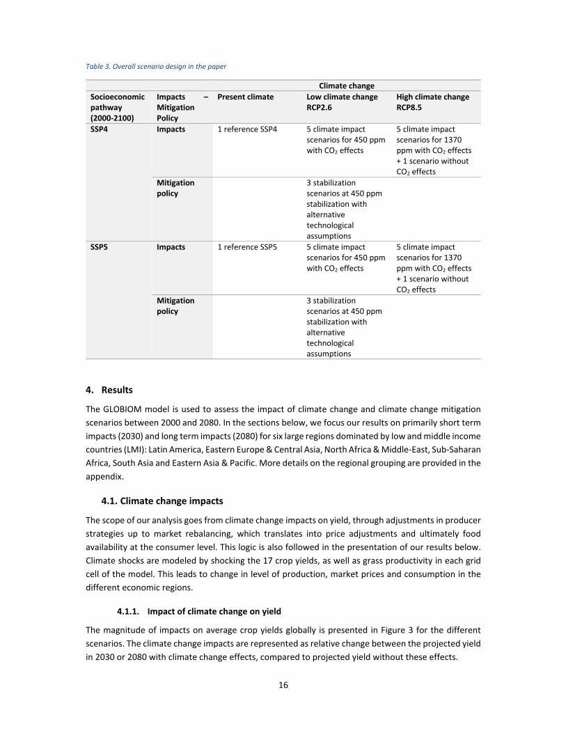
4. Results 

The GLOBIOM model  is used to assess the  impact of climate change and climate change mitigation 

scenarios between 2000 and 2080. In the sections below, we focus our results on primarily short term 

impacts (2030) and long term impacts (2080) for six large regions dominated by low and middle income 

countries (LMI): Latin America, Eastern Europe & Central Asia, North Africa & Middle‐East, Sub‐Saharan 

Africa, South Asia and Eastern Asia & Pacific. More details on the regional grouping are provided in the 

appendix.  

4.1. Climate change impacts 

The scope of our analysis goes from climate change impacts on yield, through adjustments in producer 

strategies  up  to market  rebalancing, which  translates  into  price  adjustments  and  ultimately  food 

availability at the consumer level. This logic is also followed in the presentation of our results below. 

Climate shocks are modeled by shocking the 17 crop yields, as well as grass productivity in each grid 

cell of the model. This leads to change in level of production, market prices and consumption in the 

different economic regions. 

4.1.1. Impact of climate change on yield  

The magnitude of  impacts on average crop yields globally  is presented  in Figure 3  for the different 

scenarios. The climate change impacts are represented as relative change between the projected yield 

in 2030 or 2080 with climate change effects, compared to projected yield without these effects. 

17  

At the horizon 2030, the impact of climate change, when CO2 effects are considered, is expected on 

average to be of ‐1.8% under RCP 2.6 and ‐2.9% under RCP 8.5. The two sets of RCPs differ more by 

GCM at this time horizon, because the scenarios diverge only after 2010 and GHG concentrations are 

still close to each other in 2030. Furthermore, the delay between effective reduction of GHG emissions 

and climate change response limits the possibilities to influence climate change at such a short time 

horizon, which  impedes  heavily  to  historical  emissions.  The  HadGEM2‐ES  and MIROC‐ESM‐CHEM 

models have the largest average impacts, with ‐5.0% and ‐5.1% respectively. When CO2 effects are not 

considered (only analyzed with HadGEM2‐ES here), the impacts are found to be more significant at ‐

10.2%. 

The impact of different levels of radiative forcing is much more pronounced when looking at the long‐

term developments. By  2080,  the  average  impact under  strong  climate  change  (RCP  8.5)  reaches 

globally ‐13.9% by 2080 when CO2 effects are considered (max. MIROC‐ESM‐CHEM at ‐20.2%). Under 

limited climate change (RCP 2.6), effects remain rather stable, close to their 2030 range of impact, with 

average  at  ‐1.8%  in  2080.  Some  positive  impacts  are  even  observed  for  two  climate  models. 

Considering a strong climate change with no CO2 effects leads to strongly negative crop yield impacts, 

reaching ‐32.7% globally by 2080 (red bar). 

 

Figure 3. Climate change impact on average crop yield at global level in 2030 and 2080 for different climate scenarios and climate models. Crops correspond to the 18 species represented in the GLOBIOM model and impacts are aggregated on a dry matter yield basis. 

Looking at the regional patterns, some contrasting situations appear for the different regions  in the 

world  (Figure  4).  Latin  America,  South  Asia,  Sub‐Saharan  Africa  and  Eastern  Asia  &  Pacific  are 

consistently found to suffer  in terms of crop yields by 2080, for RCP 8.5 with CO2 effects, whatever 

GCM results are considered. Impacts can be as severe as ‐23.3% for South Asia, and reach on average 

‐17.4% for Eastern Asia & Pacific, ‐15.2% for Sub‐Saharan Africa and ‐13.9% for Latin America. Other 

regions experience positive yield impacts due to CO2 effects. Middle‐East & North Africa yields increase 

18  

on average by 7.8% in RCP 8.5 and Eastern Europe and Central Asia gain 9.2% by 2080.5 This picture 

seems to be relatively robust over time, since similar spatial patterns can be found by 2030, although 

impacts are of much lower magnitude. 

If CO2 effects do not materialize, overall impacts are more severe and all regions experience negative 

yield changes. Effects are found particularly dramatic for most affected regions under RCP 8.5 with CO2 

effects, by 2080. Eastern Asia & Pacific lose ‐37.1% in crop yield whereas impacts in South Asia reach ‐

34.6%. Yields in Sub‐Saharan Africa are also substantially affected with an average impact of ‐29%.  

 

Figure 4. Climate change impact on average crop yield for six regions in 2080 for different climate scenarios and climate models. Crops correspond to the 18 species represented in the GLOBIOM model and impacts are aggregated on a dry matter yield basis. For results in 2030 see figure D‐1 in appendix D. 

Within each  region,  crops are also differently affected. Figure 5  illustrates  the  contrasted  impacts 

under  the RCP 8.5  scenario, when CO2 effects  are  taken  into  account. Depending on  the  regional 

patterns of climate change and on where and under what management a crop is grown, impacts can 

vary widely. For instance, wheat, which is very severely impacted in Eastern Asia & Pacific (‐29.9%) is 

impacted positively in all other regions. Rice is impacted negatively in Sub‐Saharan Africa (‐8.6%) but 

positively in North Africa and Middle‐East (+12.0%). Some crops are particularly hit across all regions, 

such as potatoes (up to ‐65% in Sub‐Saharan Africa), groundnuts (up to ‐49.1% in Sub‐Saharan Africa) 

or cotton (up to ‐50.6% in Eastern Asia & Pacific). 

                                                            5MENA region sees the highest difference worldwide in yield response with and without CO2 effects (resp. +6% and ‐20%, see figure 4), and illustrates the particularities of elevated CO2 concentration impacts: in addition to increasing photosynthesis rate for a given level of incoming solar radiation (fertilization effect), increasing CO2 directly increases crop water‐use efficiency. Such an effect is included in most state‐of‐the‐art crop models, and can significantly alleviate water constrains to production. In the case of MENA, it counterbalances robust but relatively small decreases in precipitation. Further details on how water affects crop yield and irrigation developments in GLOBIOM are documented in Leclère et al. (2014). 

19  

 

Figure 5. Climate change impact on by crop for six regions in 2080 for the RCP 8.5 scenario with CO2 effects. Impacts are averaged across the five GCMs in the analysis. Only crops with cultivated areas greater than 100,000 ha in 2000 are represented. Crop acronyms:  WHEA= wheat, RICE = rice, CORN = corn, SOYA = soybean, RAPE = rapeseed, BARL = barley, CASS = cassava, SUNF = sunflower, MILL = millet, SRGH = sorghum, SUGC = sugar cane, BEAD = dry beans, COTT = cottonseed, CHKP = chick peas, SWPO = sweet potatoes, POTA = potatoes, GNUT = groundnuts. For results in 2030 see figure D‐2 in appendix D. 

4.1.2. Adaptation responses along the supply chain 

Climate change  impacts on crop yields affect agricultural output  in the different regions and pose a 

challenge  for  overall  food  availability.6  Figure  6  illustrates  the  chain  reaction  triggered  in  the 

agricultural markets by the biophysical yield shocks in 2030 and 2080. For each economic variable, the 

relative change to the baseline value  is shown, which allows attribution of the different sources of 

adaptation.  Adaptation  responses  increase with  the  size  of  the  shock  and  allow  alleviation  of  a 

significant part of the shock. 

First of all,  farmers adapt their management  (fertilizer  input system,  irrigation)  in response to crop 

productivity change and the final yield decrease is therefore lower than the initial biophysical shock. 

Some regional reallocation within each region can also take place and is reflected in the response of 

this variable. Adaptation also occurs through harvested area adjustments, made necessary to maintain 

sufficient production under lower yields and to make use of the new opportunities. In 2030 and 2080, 

harvested areas increase, and partly compensate the effect of yield decrease. As a consequence, the 

overall impact of climate change on production is smaller than the initial biophysical shock. 

Second, countries buffer their deficit of production by trade adjustments. This can be illustrated by the 

indicator of trade share, defined here as the ratio of net trade over regional market size (here, the 

                                                            6 Note that in the rest of paper, we will refer indifferently to food availability or to food consumption to designate the quantity of food supplied to households for their domestic use. This includes effective ingestion of food by human beings but also domestic food waste. 

20  

average of production and consumption in the baseline).7 At the global level and aggregated across all 

crops, these effects remain limited and marginal in 2030. But as climate change becomes more severe, 

trade  appears  as  an  important  contributor  to  adaptation. The  adjustments  through  trade  in 2080 

represent  0.4%  and  1.2%  of  the  global  production  under  RCP  8.5 with  and without  CO2  effects, 

respectively, between the ten different macro‐regions considered here. This is equivalent to average 

extra trade flows of 120 and 260 million tonnes dry matter, respectively, between these regions.8 

Third, the consumption side adapts to the change in prices. Food consumption decreases, with some 

socioeconomic implications – see subsection 4.1.4 for more results – but feed consumption decreases 

even more, because it is more price elastic. This adjustment on the feed side also limits the food impact 

of the losses on the production side, as a larger part of the production can be allocated to food use.   

 

Figure 6. Propagation of climate change impact along the chain of economic indicators in 2030 and 2080 across different climate scenarios. CC shock corresponds to the average biophysical impact of climate change on dry matter yield; Yield corresponds to final resulting dry matter yield, including adaptation response; Area is the total change in harvested area; Prod is the change in total crop production in dry matter basis; Price is the average crop price index; Trade sh. corresponds to difference in the share of interregional trade (export – import) in total crop production; conso is the change in total crop consumption, and food and feed the relative change in the consumption of food and feed. The average responses for the five GCM models and the two SSP4 and SSP5 scenario are considered. For RCP8.5* sensitivity analysis, only the HadGEM2‐ES GCM is featured. Units are average relative change to the baseline. 

At the level of the different regions, similar dynamics of response are observed, as illustrated in Figure 

7 with the case of RCP 8.5 with CO2 effects. Yield management and harvested areas are used to buffer 

the adverse effect of climate change on the supply side, and trade and consumption responses help to 

accommodate the impacts on production.  

The magnitude of effects and responses however differs depending on the region. In Latin America, 

South Asia and Eastern Asia & Pacific, area adjustments are strong and allow for a partial compensation 

                                                            7 Market share in the graphs are compared with the baseline as difference (and not in relative change). As a consequence, one percent increase in market share indicator means that net trade increased and provided the equivalent of 1% of the production or consumption. As net trade flows cancel at global level, the indicator for world is calculated by accounting only the net trade flows between regions that are positive. 8 Intra‐region trade flows are not presented here. 

21  

of the yield effect. Area changes have a more  limited role  in the two African regions, particularly  in 

Sub‐Saharan Africa where smallholders have more difficulties to adapt.  In Latin America or Eastern 

Asia & Pacific, little change in food consumption is observed, whereas these impacts are important in 

Sub‐Saharan Africa and in South Asia. 

Trade pattern differences are also very visible in Figure 7. Regions with increases in production (Latin 

America, Middle East and North Africa, Eastern Europe and Central Asia) export more, whereas regions 

with decreases in production (South Asia, Sub‐Saharan Africa and, to a lower extent, Eastern Asia & 

Pacific)  use  imports  to  buffer  a  part  of  the  effects  on  production.  Interestingly,  the  different 

specifications  for  the  two  SSPs  are well  reflected  in  the  trade  results. Under  SSP4  (red),  trade  is 

considered  relatively  constrained and  trade adjustments  remain  low. Under SSP5  (blue), observed 

responses are much  larger and partly help  to mitigate price  impacts,  for  instance  in South Asia or 

Eastern Asia & Pacific, or provide export opportunities to relatively less affected regions (Latin America, 

Eastern Europe and Central Asia). 

 

Figure 7. Propagation of climate change impact along the chain of economic indicators for SSP4 and SSP5 in 2080 for RCP 8.5 with CO2 effects. CC shock corresponds to the average biophysical impact of climate change on dry matter yield; Yield corresponds to final resulting dry matter yield, including adaptation response; Area is the total change in harvested area; Prod is the change in total crop production in dry matter basis; Price is the average crop price index; Trade sh. corresponds to difference in the share of interregional trade (export – import) in total crop production; conso is the change in total crop consumption, and food and feed the relative change in the consumption of food and feed. The average responses for the five GCM models are considered. Units are relative change to the baseline. For results in 2030 see figure D‐3 in appendix D. 

22  

4.1.3. Crop and livestock sector impacts 

The different agricultural sectors will be affected with different  levels of severity depending on the 

region but also on  the activity  type. Figure 8 shows with  this  respect  the contrast  in situations  for 

different types of farm production. 

  

Figure 8. Change in production of different products for different climate change scenarios under SSP4Crops are aggregated by dry matter tonnes, meat by animal carcass weight, and milk by volume. The average responses for the five GCM models are considered except for the RCP8.5* sensitivity analysis, based on the HadGEM2‐ES GCM. 

For the crop sectors, as emphasized in the previous section, farmers can mitigate a part of the yield 

shock by adapting their management to the effect of climate change, which leads to lower shocks on 

final yields. They also mitigate the loss of productivity by expanding harvested areas, where possible. 

Overall impacts of climate change on crop supply are therefore found less severe as suggested by yield 

impact. In 2080, the impact of climate change under RCP 8.5 on crop production is ‐5.6% and ‐10.4% 

with and without CO2 effects, respectively. 

Changes in the production of the different livestock sectors depend on their link with the crop sectors, 

and also on the impact of climate change on grassland (Havlík et al., 2015). The pig and poultry sectors 

depend heavily on grain concentrates and the impact of climate change on crops hit this sector directly 

through  the  feed channel. As a consequence, pig and poultry production under RCP 8.5 decreases 

globally by ‐3.4% and ‐7.4% with and without CO2 effects, respectively. Ruminant animals benefit from 

the increased grass productivity under scenarios with CO2 effects. Therefore, beef, lamb and goat meat 

output increase by 3.1% in 2080 under RCP 8.5, whereas milk output rises by 0.9%. However, without 

CO2 effects, grass and crop productivities are both negatively affected, and the two sectors decrease 

their production by ‐1.9% and ‐2.0% by 2080. 

4.1.4. Socioeconomic impacts 

Agricultural prices are a  sensitive parameter when examining poverty  impacts. Even when  food  is 

produced  in sufficient quantity overall, problems of distribution and access can  lead  to prohibitive 

prices in some regions, preventing the poorest from meeting their minimum needs and leading to food 

insecurity in absence of social programs or safety nets.  

Agricultural prices are projected  in our model to only moderately grow until 2030 for the two SSPs 

without climate change. Crop and livestock product prices increase by 7% and 9%, respectively, under 

23  

the SSP4 reference scenario by that time horizon. Under SSP5, the change would be even lower, with 

a stable price for crops and +5% for livestock commodities. Differences come mostly from the faster 

technological growth and  international market  integration  in SSP5. The market  integration effect  is 

very significant also for the regional prices. While under SSP5, crop prices vary between ‐1% in Eastern 

Europe & Central Asia and 4% in Sub‐Saharan Africa, the same prices still stagnate for the former under 

SSP4, but grow by 24% for the latter due to increased market isolation. 

Under climate change, producer prices increase for sectors negatively impacted, and the effects are 

much more  severe  under  high  climate  change  –  and  even more  so when  CO2  fertilization  is  not 

considered. The magnitude of price response is also determined by the capacity of regions to adjust to 

the different adaptation channels, as illustrated by the previous section. Therefore, and in spite of the 

possibility of aligning prices to international price for the most traded products, price changes do not 

affect  all  regions  in  the  same  way  (see  Figure  9).  Patterns  also  vary  significantly  between 

socioeconomic scenarios, because levels of development are not the same in each region. For instance, 

Sub‐Saharan Africa is the most severely impacted region under SSP4 with up to an 11.9% increase in 

crop prices in 2030 for RCP 8.5 without CO2 effects. Impacts in this region are relatively less severe for 

the same scenario under SSP5, with a 5.6% price increase. This can be explained by the more restricted 

trade  conditions  under  SSP4.  A  similar  difference  between  the  two  socioeconomic  scenarios  is 

observed in the case of South Asia.  

 

Figure 9. Climate change impact on agricultural prices in 2030 at regional level for different climate scenarios under SSP4 (left bar group in each panel) and SSP5 (right bar group). Price indexes are aggregated across crops using 2000 base year production. The average responses for the five GCM models are considered except for the RCP8.5* sensitivity analysis, based on the HadGEM2‐ES GCM. 

Without climate change, food demand is projected to grow by 4% and 11% between 2000 and 2030, 

under  SSP4  and  SSP5, which  corresponds  to  increases  from  2700  kilocalories  per  capita  per  day 

(kcal/cap/day) to 2800 and 3000 kcal/cap/day, respectively. While under SSP4, the increase would be 

the strongest in East Europe & Central Asia, +241 kcal/cap/day, under SSP5, it would be the strongest 

24  

in Sub‐Saharan Africa, +645 kcal/cap/day, showing nicely the economic and technological catching up 

of  the  region.  If  these  trends  are  strongly  shaped  by  the  effect  of  economic  growth,  prices  also 

determine directly the final level of food consumption, and GLOBIOM represents a log linear response 

for each product between prices and consumption level. The overall global impacts of climate change 

on food consumption can be observed in Figure 10. Impacts are very limited for low climate change 

(RCP  2.6)  but  for  high  climate  change,  impacts  on  food  consumption  become  progressively more 

severe over time, culminating for SSP4 at ‐4.4% with CO2 effects and at ‐8.7% without CO2 effects (left 

panel). This latter case results in a complete stagnation of calorie consumption globally compared to 

the present day  situation  (+30  kcal/cap/day between 2080 and 2000) and effects  are much more 

dramatic in developing regions, with for example a decrease by 79% of additional food availability per 

capita in Sub‐Saharan Africa. 

Under SSP5, the impacts of climate change on food consumption are found to be much lower, which 

is fully consistent with the previous observation of lower price changes. Larger trade adjustments in 

SSP5 reinforce adaptation responses and minimize price responses in this scenario. Impacts therefore 

remain  at  a  level  of  ‐2.8%  and  ‐4.3%  under  RCP  8.5 with  and without  CO2  effects,  respectively. 

Additionally, demand becomes more inelastic over time as the different regions develop and this effect 

is much  stronger  under  SSP5,  where  a  faster  economic  growth  is  assumed.  As  a  consequence, 

differences in magnitude of impacts tend to be more visible in 2080 than in 2030 or 2050. Impacts of 

climate change materialise here  in a context where food  is much more abundant than  in SSP4, and 

therefore, even in the worst climate change scenario, the final food consumption per capita by 2080 

is 3,429 kcal globally, which is comparable to the present day levels of consumption in Europe. 

 

 

Figure 10. Climate change impact on global food consumption at different time horizon for different climate scenarios under SSP4 (left) and SSP5 (right). Food products are aggregated by their calorie content. The average responses for the five GCM models are considered except for the RCP8.5* sensitivity analysis, based on the HadGEM2‐ES GCM. 

25  

The regional impacts of the different scenarios illustrate the contrasting fortunes of different regions 

(Figure 11  for the short term impacts in 2030). Regions that are found to be the most affected are Sub‐

Saharan Africa, South Asia and Eastern Asia & Pacific. The differentiated effects on food consumption 

reflect the heterogeneity in regional results on food prices, but also the different specificities of diets. 

For  instance, Latin America, which  relies on a diversified diet where animal based products play a 

significant role, is less affected than South Asia where diets are mostly based on some vulnerable crops, 

such as rice, wheat, sorghum, potato. 

Another  important source of differences  is the values of price elasticities of demand which vary for 

each region (larger for least advanced countries). Developed countries also experience higher prices 

(not in figure) but they react much less on the food demand side. For instance, for an 11.9% increase 

in crop prices in Sub‐Saharan Africa in 2030 (RCP 8.5 without CO2 effects), food consumption decreases 

by 5.2%. At the same time in North America, prices increase by 18.2% but food consumption decreases 

only by 1.4%. 

 

Figure 11. Climate change impact on food consumption per capita in 2030 for different climate scenarios under SSP4 (left bar group in each panel) and SSP5 (right bar group) at regional level. Food products are aggregated by their calorie content. The average responses for the five GCM models are considered except for the RCP8.5* sensitivity analysis, based on the HadGEM2‐ES GCM. 

4.2. Climate change mitigation 

While  it seems  that without additional measures humanity  is well on  track to reach GHG emission 

levels corresponding to RCP8.5, stabilizing the emissions at levels compatible with RCP2.6 will require 

substantial mitigation efforts. In this sub‐section, we present three alternative levels of effort in terms 

of  mitigation  of  AFOLU  emissions  and  biomass  supply  corresponding  to  different  technological 

assumptions, but compatible with climate change stabilization at the RCP2.6 level. There are several 

mechanisms through which the idealized mitigation policy considered here will impact the agricultural 

and forest sectors; carbon prices will increase the production cost of GHG emitting activities, and the 

26  

demand for GHG reducing activities, like afforestation and biomass for energy production, will increase 

the competition for resources, in particular for land. As for climate change impacts, these changes in 

agricultural and forestry markets can affect commodity prices and food availability. 

4.2.1. Emissions from agriculture, forestry and other land use (AFOLU) 

By 2000, AFOLU emissions, as accounted for in GLOBIOM, amounted to some 11 GtCO2e globally, of 

which about 60% came from land use change. Figure 12 shows how these emissions are distributed 

across different  regions.  Latin America, Sub‐Saharan Africa and Eastern Asia & Pacific  represented 

together 77% of  total AFOLU emissions  in 2000. These numbers are well  in  line with  the  recently 

reported  levels by Smith et al. (2014) who estimated total average AFOLU emissions for the period 

2000‐2010 at 10‐12 GtCO2e per year, with emissions from agriculture amounting to 5.0‐5.8 GtCO2e per 

year and emissions from land use and land use change amounting to some 4.3‐5.5 GtCO2e per year. 

Even without climate change policy, net emissions from forestry and other land use would under SSP4 

go  down  by  24%  between  2000  and  2030.  At  the  same  time,  direct,  non‐CO2,  emissions  from 

agriculture would increase by 28%, leading to overall AFOLU emissions reduction by 5%. Under SSP5, 

similar reduction in emissions from land use change is projected. However, because of the sustained 

food demand,  in particular for  livestock products, non‐CO2 emissions from agriculture would be 4% 

higher by 2030 than under SSP4. The difference between SSPs is getting more pronounced over time. 

For  instance under SSP4 by 2080, AFOLU emissions are projected to decrease by 49% compared to 

2000, while under SSP5, the AFOLU emissions would be 25% higher compared to the same year under 

SSP4. 

 

Figure 12 GHG emissions in 2030 from agriculture, forestry and other land use in the reference and the different mitigation scenarios, at global and regional  level [GtCO2e]. The first bar of each panel corresponds to the base year 2000 calibration results. 

In the climate stabilization scenario with Full Technology (FullTech) assumption, AFOLU emissions as 

calculated by GLOBIOM would decrease by 58% compared to the reference level by 2030 under the 

27  

SSP4 scenario. This result is consistent with the EMF27 results themselves, where the models estimate 

that under this stabilization scenario, AFOLU emissions would need to be reduced by ‐4% to 99% (Smith 

et al., 2014). According to our results, Latin America, Sub‐Saharan Africa and Eastern Asia & Pacific 

would contribute 45%, 26% and 13% of the global AFOLU abatement, respectively, providing together 

the large majority of the global mitigation effort in this sector. Under this stabilization scenario, direct 

emissions from agriculture remain roughly at their 2000 level, and net emissions from land use change 

approach  zero,  mostly  because  of  reduced  emissions  from  deforestation  accompanied  by 

afforestation. As one would expect, under the Low Energy Intensity scenario (LowEI), less mitigation 

effort is required from the AFOLU sector; total AFOLU emissions would then be about 20% higher than 

under FullTech. With limited role of bioenergy in the mitigation portfolio (LimBio scenario), agricultural 

emissions would be required to go even lower than under FullTech, and land use change would need 

to become a net sink of emissions already in 2030. This shows the need for substitution of negative 

emissions from bioenergy with carbon capture and storage by negative emissions from afforestation 

in order to achieve the climate stabilization. 

4.2.2. Biomass supply for energy 

Total amount of bioenergy is in the reference scenario without mitigation policy projected to slowly 

decrease until 2050 because of the decreasing importance of traditional fuelwood use, and to start to 

increase  afterwards  because  modern  bioenergy  becomes  competitive  even  without  mitigation 

policies. Figure 13 provides an overview of how biomass supply for bioenergy would develop under 

stabilization scenarios. In the FullTech stabilization scenario, demand for bioenergy by 2030 would be 

multiplied by two compared to the reference scenario. Sub‐Saharan Africa, Latin America and Eastern 

Asia &  Pacific would  again  be  important  players  supplying  each  about  20%  of  the  total  biomass 

demand. This result is in line with the findings by Rose et al. (2012) that up to 80% of the biomass for 

energy production would come from non‐OECD countries. With respect to the source of the biomass, 

our projections suggest that while in Latin America the quasi‐totality of the biomass would come from 

dedicated plantations, in Sub‐Saharan Africa and Eastern Asia & Pacific, 30%, respectively 20%, of the 

total biomass would come from traditional forests. This differentiation is due to high plantation yields 

and large areas of suitable land in the case of Latin America, and vast areas of tropical forests where 

currently only a  small  fraction of  the biomass, high quality woods,  is extracted  from  the managed 

zones. The required biomass supply would be 43% lower in the LowEI scenario, and, it would be 15% 

lower  also under  the  LimBio  scenario.  The  demand  for biomass  is projected  to  continue  to  grow 

substantially beyond 2030. Under  the  FullTech  scenario, biomass demand would more  than  triple 

between 2030 and 2080. This new demand represents future income opportunities in the forestry and 

agricultural sectors.  

28  

 

Figure 13 Biomass supply for energy production in 2030 for SSP4 and SSP5 in the reference and in the alternative stabilization scenarios [EJ primary energy per year].  

4.2.3. Crop and livestock production 

Crop production for the 17 products in the model represented 2.4 Gt dry matter in 2000. It is projected 

to grow without mitigation policies by an additional 1.4 Gt and 1.7 Gt for SSP4 and SSP5 respectively, 

between  2000  and  2030.  The  growth  is  projected  to  be  particularly  high  due  to  income  growth, 

population  growth  and  changes  in  preferences  in  developing  regions  under  SSP5  where  diet 

preferences converge towards more Western trends. Hence, in South Asia crop production is projected 

to grow by 307 Mt (340 Mt), in Middle East & North Africa by 69 Mt (60 Mt) and in Sub‐Saharan Africa 

by 171 Mt (197 Mt) for SSP4 (SSP5). Climate stabilization efforts would substantially impact the crop 

production growth, as illustrated in Figure 14. In Sub‐Saharan Africa, the production growth would be  

9% (13%) lower under FullTech than under the reference scenario, and even by 12% (14%) lower under 

the LimBio scenario, leading potentially to decreases in farmers income and less food available for the 

consumers. It is interesting to note that even under the LimBio scenario for SSP5, the total production 

is higher than in the reference scenario for SSP4. 

29  

 

Figure 14 Difference in crop production levels between 2000 and 2030 in the reference and alternative stabilization scenarios, at global and regional level, under different SSPs [million dry matter tonne]. Full product definitions in Appendix. 

As for crop production, livestock production is also subject to a strong global increase in the reference 

scenario, from 53 Mt of protein supply in 2000 to 82 Mt in 2030 under SSP4, and 90 Mt under SSP5. 

Developing regions again show the largest increases leading to a more than doubling of the production 

in Sub‐Saharan Africa, South Asia and Mid East & North Africa. As shown  in Figure 15, the  livestock 

sector would be directly impacted by the mitigation policy, but all sub‐sectors would not be affected 

equally; depending on the technology scenario, ruminant meat production would decrease, by 6 to 

16% relative to the reference scenario. Poultry meat production would decrease by maximum 2%. This 

comes from the relative GHG emissions (in)efficiency of the different sub‐sectors (de Vries and de Boer, 

2010), which  implies that ruminant meat production  is much more affected by a carbon price than 

poultry production. While the relative effect of the climate stabilization scenarios is similar under SSP4 

and  SSP5,  because  of  the  larger  growth  in  the  reference  scenario  in  SSP5,  the  global  livestock 

production in the latter scenario would remain above the reference level of SSP4 in all the technology 

scenarios. 

30  

 

Figure 15 Difference in livestock product output between 2000 and 2030 in the reference SSP4 and SSP5 and the alternative stabilization scenarios, at global and regional level [million tonnes proteins]. 

GHG  emission  efficiency  also  largely  varies  within  each  livestock  sub‐sector  depending  on  the 

production system (Herrero et al., 2013). The differences are particularly large in the ruminant sector, 

and a carbon tax would lead to significant reallocation of production from extensive grazing systems 

to (semi‐) intensive mixed systems (Havlík et al., 2014). Reallocations across livestock systems for the 

different mitigation scenarios are visible in Figure 16. The share of beef supply coming from grazing 

systems  (“LG”  in the  figure) would be  in  the mitigation scenarios under SSP4 around 5 percentage 

points lower by 2030 than in the reference scenario, 12% compared to 17%. In Sub‐Saharan Africa the 

share of  intensive mixed  systems  (“MRT”  in  the  figure)  in beef production would be 4 percentage 

points higher  in the stabilization scenarios than  in the reference, 29% as compared to 25%. Similar 

observations hold in the case of SSP5. An enabling environment needs to be created to support such 

intensification of extensive systems, or where biophysical conditions do not allow for this, alternative 

sources of income need to be proposed to the pastoralists. 

 

31  

 

Figure  16  Difference  in  shares  of  beef  production  allocation  to  different  production  systems  in  2030  for  the  different stabilization  scenarios,  compared  to  the  reference SSP4 or SSP5  [percentage points].  (LGA – grazing  systems arid,  LGH – grazing systems humid, LGT – grazing systems temperate and in tropical highlands, MRA – mixed crop‐livestock systems arid, MRH –mixed crop‐livestock systems humid, MRT – mixed crop‐livestock systems temperate and in tropical highlands).  

4.2.4. Forest sector production 

Industrial round wood supply  is projected to  increase by 49%  (61%)  in the reference scenario SSP4 

(SSP5) by 2030. Globally, the different variants of stabilization scenarios have very limited impact on 

round wood supply, Figure 17. Regionally, we can see some significant differences. In LAM, FullTech 

scenario leads to a slightly increased round wood supply, +5% in SSP5, which can be traced back to the 

increased  value of  forest based by‐products  and  thereby  lowering  the  cost of producing  the  final 

timber products. On the other hand, mitigation under the FullTech scenario  leads to reduced round 

wood  supply  in  Eastern  Europe  &  Central  Asia,  because  of  substantial  sourcing  of  biomass  for 

bioenergy from the traditional forests and limited potentials to increase the total forest harvest level. 

In this region, we also clearly see the differentiated impact of increased biomass demand on pulpwood 

and saw logs supply. Pulpwood can be either main product from the forest, or, more often, it is a lower 

grade by‐product of saw logs harvesting. Both saw logs and pulpwood type of biomass can be used for 

energy production. Hence, while the energy feedstock can be a by‐product of saw logs harvesting, and 

so  improve  the  economics  of  the  latter  leading  to  an  increased  supply,  it  is  direct  competitor  to 

pulpwood production. 

32  

 

Figure 17 Difference in industrial roundwood production between 2000 and 2030 for the reference SSP4 and SSP5 and the alternative stabilization scenarios, across wood type products [million cubic meters]. 

4.2.5. Land cover change 

Land cover development is a good aggregate indicator of the change in agriculture, forestry and other 

land  use,  and  illustrates  the  transformational  challenges  implied  by  the  ambitious  stabilization 

scenarios. Under the reference scenario SSP4, cropland is projected to expand by 58 million hectares, 

grassland by 117 million hectares, and dedicated energy plantations by 82 million hectares between 

2000 and 2030 (Figure 18). 78% of cropland expansion would occur in Sub‐Saharan Africa, grassland 

expansion would be shared mostly by Eastern Asia & Pacific, Sub‐Saharan Africa, and Latin America, 

and plantations expansion would be similar across the regions. About one third of the newly cultivated 

land would  come  from  former  forests,  and  two  thirds  from  other  natural  vegetation.  The major 

difference  under  SSP5  would  be  the  30%  higher  expansion  of  grasslands  due  to  the  economic 

development and shifts in diet preferences. 

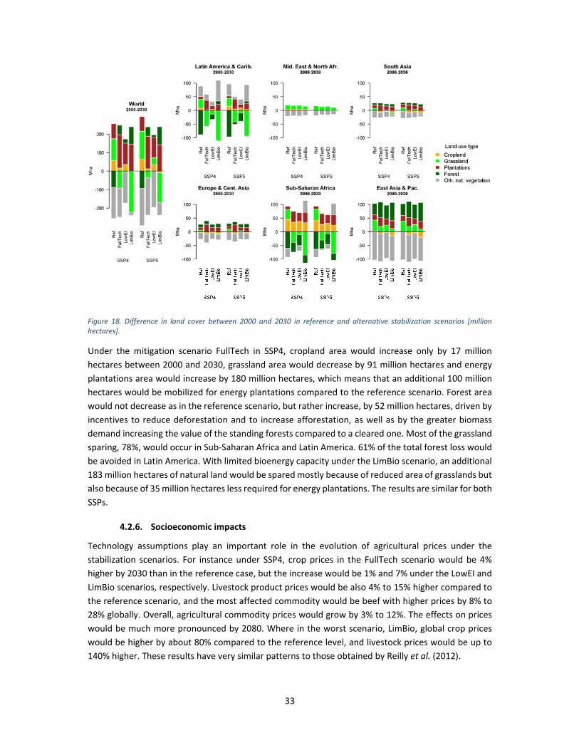
33  

 

Figure  18. Difference  in  land  cover  between  2000  and  2030  in  reference  and  alternative  stabilization  scenarios  [million hectares]. 

Under  the mitigation  scenario  FullTech  in  SSP4,  cropland  area would  increase  only  by  17 million 

hectares between 2000 and 2030, grassland area would decrease by 91 million hectares and energy 

plantations area would increase by 180 million hectares, which means that an additional 100 million 

hectares would be mobilized for energy plantations compared to the reference scenario. Forest area 

would not decrease as in the reference scenario, but rather increase, by 52 million hectares, driven by 

incentives to reduce deforestation and to  increase afforestation, as well as by the greater biomass 

demand increasing the value of the standing forests compared to a cleared one. Most of the grassland 

sparing, 78%, would occur in Sub‐Saharan Africa and Latin America. 61% of the total forest loss would 

be avoided in Latin America. With limited bioenergy capacity under the LimBio scenario, an additional 

183 million hectares of natural land would be spared mostly because of reduced area of grasslands but 

also because of 35 million hectares less required for energy plantations. The results are similar for both 

SSPs. 

4.2.6. Socioeconomic impacts 

Technology  assumptions  play  an  important  role  in  the  evolution  of  agricultural  prices  under  the 

stabilization  scenarios. For  instance under SSP4,  crop prices  in  the FullTech  scenario would be 4% 

higher by 2030 than in the reference case, but the increase would be 1% and 7% under the LowEI and 

LimBio scenarios, respectively. Livestock product prices would be also 4% to 15% higher compared to 

the reference scenario, and the most affected commodity would be beef with higher prices by 8% to 

28% globally. Overall, agricultural commodity prices would grow by 3% to 12%. The effects on prices 

would be much more pronounced by 2080. Where  in the worst scenario, LimBio, global crop prices 

would be higher by about 80% compared to the reference level, and livestock prices would be up to 

140% higher. These results have very similar patterns to those obtained by Reilly et al. (2012).  

34  

The  rather moderate  aggregate  effects  by  2030  can  be more  pronounced  on  the  regional  level, 

reflecting the relative GHG efficiency of the different regions (Figure 19). For instance, while beef prices 

would increase by just about 10% in Western Europe or North America, they would increase by more 

than  40%  in  Latin  America  and  in  Sub‐Saharan  Africa  under  the  FullTech  scenario,  with  strong 

implications  for  local  consumers.  Regional  results  also  reveal  different  patterns  across  SSPs,  in 

particular for Latin America and Asian regions. SSP5 impacts are in these cases relatively higher than 

in SSP4 for all stabilization scenarios. This is due in particular to the higher share of livestock products 

in human diets, whose prices are strongly hit by the mitigation measures. 

 

Figure 19 Change in food prices in the different stabilization scenarios compared to the reference SSP4 and SSP5, at global and regional level [%].Price indexes are aggregated across crops and livestock product using 2000 base year production. 

Price increases in the mitigation scenarios are related both to the increased competition for land for 

carbon sequestration (afforestation, avoided deforestation) and for biomass production, as well as to 

the  carbon  tax  directly  increasing  the  production  costs. Overall  impacts  on  farmer  revenues will 

depend on whether they can benefit from the increased land rent (Zekarias et al., 2013) and on their 

GHG emissions efficiency which will become a part of their comparative advantage. On the consumer 

side, however, such mitigation policies would have negative effects on food availability through the 

increased food prices. 

When looking at final food availability, the impact of agricultural prices appears strong for all mitigation 

scenarios (see Figure 20). The mitigation scenario FullTech, would reduce the global food availability 

growth by 68% under SSP4 and by 27% under SSP5. In the scenario with limited bioenergy availability, 

LimBio, food availability in 2030 would be under the SSP4 scenario even slightly lower than in 2000.  

35  

  

Figure 20 Relative change in global food consumption level in the alternative stabilization scenarios compared to the reference by 2030 [kcal per capita per day]. Both crop and livestock products are considered. 

Regional  patterns  illustrate  the  differentiated  impacts  between  regions  with  high  food  demand 

resilience and more vulnerable ones (Figure 21). While North America, Western Europe and Developed 

Pacific would see food availability reduced by less than 1% under FullTech compared to the reference, 

LMI regions would be affected by a reduction between 2 and 3% already in 2030. The impacts are even 

higher  for the LimBio scenario, with around 5% of consumption  loss  for South Asia, Eastern Asia & 

Pacific and Sub‐Saharan Africa. Overall,  the effects of mitigation policies on  food availability  seem 

rather small at this time horizon, but they would become more important as carbon price and demand 

for bioenergy are projected to  increase more substantially over time. For  instance under SSP4, high 

income regions would see calorie availability reduced by about 5% by 2080, and the LMI regions by 10‐

15%. 

Impacts globally appear much higher under SSP4, due to the limited possible trade adjustments and 

the more elastic demand due to  lower GDP per capita  in LMI regions. When examining to regional 

results however, effects appear more ambivalent depending on the region. Most regions are more 

severely affected by  the mitigation policies under SSP5  in  relative  terms,  to  the exception of Sub‐

Saharan Africa that experience a greater reduction of  food demand under SSP4. However, because 

food consumption for these regions is higher under SSP5 baseline (by 7% globally in 2030, and by 20% 

in  the  case  of  Sub‐Saharan  Africa),  the  same  relative  impact  from mitigation  has more  adverse 

implication under  SSP4.  For  instance,  in  Sub‐Saharan Africa,  food  availability  improvement on  the 

2000‐2030 period is reduced by 53% under FullTech with SSP4 and ends at 2345 kcal/cap/day in 2030. 

Under  FullTech with  SSP5,  the  growth  is  only  reduced  by  13%,  resulting  in  food  supply  of  2830 

kcal/cap/day in 2030. 

36  

 

Figure 21 Change in food consumption level in the different mitigation scenarios, compared to the reference SSP4 and SSP5, at regional level 

 

4.3. Comparison climate impacts vs mitigation 

Both climate change  impact and climate change mitigation were shown to affect agricultural prices 

and food consumption. However, as can be seen in Figure 22, the effects of these scenarios are rather 

limited  in the medium term.  In 2030, effects of climate change are significant only when effects of 

elevated CO2 concentration are not taken into account. For their part, stabilization scenarios lead to 

food availability losses in the range of 50‐100 kcal/cap/day, except for the case of low energy intensity. 

As observed above, the two RCPs are quite undifferentiated at that time horizon, and the effect of SSPs 

is also less discriminating.  

In  the  long  run,  food  availability would  suffer  from  the  potentially  strong  effects  of  an  idealized 

mitigation policy taxing all GHG emissions without differentiating among the sectors or regions. Such 

a policy, corresponding to a carbon price of $200 to $960 per ton of CO2e by 2080, would lead to food 

availability reduction in the range 200‐400 kcal/cap/day under SSP5, and up to 500 kcal/cap/day under 

the SSP4 scenario. Because of the higher reference level in SSP5, the food availability would with 3166 

kcal/cap/day  remain well above  the 2000  level of 2700 kcal/cap/day even  for the LimBio scenario. 

However, under SSP4, it would go down to 2592 kcal/cap/day in the FullTech scenario, and even 2440 

kcal/cap/day in the LimBio scenario, which are levels below the 2000 average value. Climate change 

impacts also show negative effects, not much differentiated across SSPs. But the food availability losses 

do not exceed 200 kcal/cap/day, and thus remain lower than losses due to climate mitigation. 

These  results  should  however  be  interpreted with  some  prudence,  due  to  the  large  number  of 

uncertainties in the climate change impacts, and to the “naive” mitigation policy design implemented 

in the model where a uniform tax is applied to all the emission sectors and its revenue stays outside of 

37  

the sector both on the producer and on the consumer side. We will discuss  in the next section the 

differential effect of including different subsets of the mitigation strategies under the tax scheme. And 

in the conclusion we will return to the discussion of the use of carbon tax revenues. 

 

Figure 22 Change in food consumption by 2030 and 2080 for all the climate change impact and stabilization scenarios compared to the reference scenario, at global level, under SSP4 and SSP5 [kcal per capita per day]. 

 

5. Discussion 

5.1. Climate change impact uncertainty  

The results in this paper provide an overview of how climate change impacts can affect different world 

regions depending on the level of greenhouse gas emissions in the future and the background socio‐

economic context. These  results need however  to be put  in perspective with other  findings of  the 

literature, owing to an important number of sources of uncertainties. 

38  

One  important source of uncertainty  is the response of the climate to change  in GHG atmospheric 

concentration, as well as the resulting patterns of change in terms of precipitation and temperature 

changes. We used in this paper results from five GCMs but a larger set of results is produced by the 

CMIP5  community  (see  full  list  and  results  overview  in  (Collins  et  al.,  2013)).  Uncertainties  for 

projections are large in these models, related to various processes difficult to model and whose net 

effect remain largely uncertain: e.g., the dynamics of cloudiness (in particular in the tropics), the role 

of surface albedo, or climate induced changes in carbon fluxes (Andrews et al., 2012; Vial et al., 2013; 

Friedlingstein  et  al.,  2014).  As  an  illustration,  although  the  projected  changes  in  global  mean 

temperature are much less uncertain compared to regional patterns or precipitation changes, CMIP5 

models estimate such a global temperature increase to range between 2.1 and 4.7 °C (Andrews et al., 

2012)  for a given degree of  radiative  forcing  (quadrupling). As detailed  in  section 3.2, our  climate 

change scenarios were specifically selected to span a large set of climate responses, and this source of 

uncertainty should be kept in mind when looking at the average results on a RCP. 

The second source of uncertainty stems from the modeling of the crop responses themselves. For this 

paper, we  relied on only one biophysical model, EPIC. However, as  illustrated  in Rosenzweig et al. 

(2014),  the most commonly used biophysical models predict very different  responses  to change  in 

temperature  and precipitation under  high  global warming. A pattern  commonly observed  in  crop 

impact research is a small increase in crop yields in high and middle latitudes under low to moderate 

global warming and negative impact in tropical areas. When large ensemble of models are compared, 

impacts by 2050 on major crops remain within the range ‐25%‐+10% for four fifths of the projections 

(Porter et al., 2014). However, when  looking at details per crop and management type (low or high 

input, irrigation), results can vary considerably depending on model parameterization (Rosenzweig et 

al., 2014). One important parameter for instance appears to be the modeling of nitrogen stress and 

the consideration of historical fertilization patterns. To this extent, our modeling framework explicitly 

takes into account the diversity of management systems and their specific response to climate change 

(Leclère et al., 2014).  

Another important source of uncertainty at the crop level is the influence of elevated atmospheric CO2 

concentration. According to the  IPCC, when CO2 effects are taken  into account, crop prices are “as 

likely as not”, with range of expected responses from ‐30% to + 45% (Porter et al., 2014). Recent studies 

illustrate that CO2 effects are not only likely to buffer a part of the impact for crops, but also to boost 

grassland productivity, with important implications for the livestock sector. Havlík et al. (2015) report 

a global average effect of climate change of +12.2% on grass yield globally using the EPIC model, and 

+45% with the LPJmL model for a RCP8.5 scenario with CO2 effects by 2050. Without CO2 effects, these 

impacts would be +2% and +7%, respectively. However, as emphasized by Rosenzweig et al., dispersion 

across model results are much higher with CO2 effects than without, and substantial additional efforts 

should be devoted to CO2 effects modeling. Additionally, there is some indication that crop quality, in 

terms of nutrient  content, may decrease under CO2  effects, which would moderate  the  expected 

benefits of yield increases (Myers et al., 2014). For these two reasons, the RCP8.5* scenario that does 

not include the effects of elevated CO2 concentration is an important counterfactual to consider in this 

paper, based here on the HadGEM2‐ES model. 

There are however some other sources of yield impacts that are absent or imperfectly represented in 

our modeling framework and could lead to either higher or lower climate change biophysical impacts. 

Some management  responses  are partially  reflected  in  a  crop model  such  as EPIC  (adjustment of 

39  

planting dates, inputs of fertilizer for high input systems, periods of harvest), but more detailed studies 

suggest that this gain could be higher, for example if including switch among existing cultivars (Leclère 

et al., 2013; Osborne et al., 2013). While this would place our results on the pessimistic range, including 

the impact of changes in water resource availability and droughts would go in the opposite direction: 

while we don’t capture them, literature based on observation has reported frequent underestimation 

of gridded simulation methods to predict crop response to extreme events (Lobell et al., 2011; Lobell 

et al., 2014). Similarly, additional negative impacts not accounted for include: rising tropospheric ozone 

concentration, and potentially higher occurrence of pests and diseases, or increased competition with 

weeds (Porter et al., 2014). Furthermore, impacts of climate change on livestock are considered here 

through  the  feed availability  channel only, whereas many other  channels  could also  influence  the 

future of the sector, in particular the role of heat and water stress on the productivity and mortality 

rate of animals, and the risk of increased spread of vector‐borne diseases (Havlík et al., 2015). 

For all the reasons above, the biophysical  impacts of climate change are subject to a relatively high 

uncertainty, although some large patterns remain observed. As an illustration, Leclère et al. (2014) try 

to  disentangle  in  their modeling  analysis  the  signal‐to‐noise  ratio  associated with  the  biophysical 

shocks coming from the climate change uncertainty. They find negative impacts on crop yield for North 

America (excl. Canada), Brazil, Sub‐Saharan Africa and most of Eastern and South Asia. However, only 

for Brazil, the signal appears higher than the noise and the negative impact considered as robust across 

scenarios. The robustness of economic response in models is for this reason limited, and is additionally 

affected by their own intrinsic parameterization uncertainty, as evidenced by the diversity of economic 

model specification and parameterization. 

Several comparison exercises  looked at how different economic models  respond  to  similar  sets of 

climate  scenarios  to  understand where  the  largest  sources  of  uncertainty  lie  in  economic  impact 

assessments.  In the  framework of the  ISI‐MIP project, Nelson et al. (2014) compared the economic 

responses  of  9  global  economic models  applied  to  agricultural  issues,  including  GLOBIOM.  They 

showed that models tend to increase the spread of biophysical input shocks when coming to variables 

such as final yield, area and production responses, but that consumption responses were much less 

dispersed  than  the  input. Models  attributed  differently  the  adjustments  to  the  shock  across  the 

different  adaptation  channels  in  the  model,  management,  expansion,  trade  and  demand.  Most 

computable general equilibrium models  (CGEs) showed  less reaction to the climate shock  (average 

below +25% after equilibrium at horizon 2050 for a RCP8.5 without CO2 effects). Partial equilibrium 

models (with the exception of GCAM) and the CGE MAGNET showed average responsiveness in prices 

above +25% for the same shock, with the strongest price sensitivity for MAGPIE (Nelson et al.), Fig S5). 

In response to price changes, adjustments differed across models, AIM, FARM, GCAM, and MAGNET 

adjusting  mainly  through  area  change,  MAGPIE  mainly  through  endogenous  yield  change,  and 

ENVISAGE, GLOBIOM, GTEM  relying almost equally on  the  two effects. Contribution  from  trade  to 

absorption of the shock was also very different across models (Nelson et al.), Fig S13 and S14): five 

models predicted limited trade adjustments (all CGEs except MAGNET, as well as MAGPIE), two models 

moderate trade adjustments (MAGNET, IMPACT) and two models large trade adjustments (GLOBIOM, 

GCAM). In the case of GLOBIOM, it is noteworthy that the trade setting for the comparison exercise is 

the same as considered for this paper for the integrated trade representation of the SSP5 scenario. 

The final impact on food consumption in Nelson et al. (2014) was estimated to be ‐3% for RCP8.5 by 

2050, under SSP2. The climate scenarios used were considered without CO2 effects but included a large 

40  

set of both climate (5) and crop (7) models    In the analysis of the present paper, using  five climate 

models and one single crop model, we obtain by 2050 a global impact of ‐4.7% for SSP4 and ‐2.8% for 

SSP5 (Figure 10). Our estimates therefore appear consistent with Nelson et al. (2014), although they 

represent for us the upper bound of our result ranges, due to the absence of CO2 effects. Geographical 

distribution of effects also show a more contrasted picture in terms of specific impact for each region, 

with Sub‐Saharan Africa and South Asia more severely hit than the world average under RCP8.5 (Figure 

23). More insight into differences across food demand responses to climate shocks is provided by Valin 

et al. (2014), which compares the same models with a deeper view on the modeling specifications of 

food demand. This paper illustrated that GLOBIOM responses in terms of food demand impact were 

similar in magnitude to those of the IMPACT model, also used in prior climate change analysis (Nelson, 

2009), but they were higher by around one half of the overall model average (Fig 8.  in (Valin et al., 

2014 ). For climate shock models derived from the LPJmL crop model, IMPACT and GLOBIOM estimated 

an  impact of food demand of ‐2% to ‐3% by 2050 compared to no climate change, whereas for the 

DSSAT crop models, impacts were at ‐5% for both models (see Müller and Robertson (2014), for the 

analysis of these crop models results). Only CGE models predicted impacts of magnitude as low as ‐

1%, with the exception of GCAM and MAGPIE which did not model demand adjustments.  

 

Figure 23. Impact on food prices of the climate change impact scenarios, at different time horizons. The colored bars indicate the average results for the 5 GCMs. The whiskers represent the range of results across the GCMs. The black dots show the results of the RCP8.5* scenario with the HadGEM2‐ES model (no CO2 effects). 

 

5.2. Trade‐offs around sector coverage of mitigation policies 

The stabilization scenarios analyzed above corresponded to an idealized mitigation policy where GHG 

emissions from all economic sectors and all regions were taxed with a unique, cost‐efficient carbon 

price  from  2010  onwards.  This  is  not  a  realistic,  and  probably  even  not  a  desirable  scenario. 

Implementation of mitigation policies  in different  regions and different  sectors  represents various 

degrees of challenge. Furthermore, ethical considerations risk of negative side effects may lead to a 

temporary  exemption of  a  region or  a  sector  from  a  general mitigation policy.  The AFOLU  sector 

together with biomass for energy production can be considered as such sensitive sectors. Agriculture 

41  

is included because of its direct link to basic human needs in terms of food but also because of being 

the main source of  livelihood  for most of the poor. Land use and  land use change are also directly 

linked with biodiversity and the poor but present considerable challenges in terms of monitoring and 

implementation in general. Havlík et al. (2014) showed how different the carbon price effects on food 

availability can be depending on whether a carbon price targets non‐CO2 emissions from agriculture 

or CO2 emissions from land use change. Finally, biomass and its potential competition with food and 

biodiversity for land and water have been extensively discussed in the literature.  

In order to get further insight in this question, we have considered three alternative scenarios to the 

idealized policy case under FullTech technology assumption: FullTechAgr – a variant of the FullTech 

scenario with bioenergy demand maintained at the level of the reference scenario without mitigation, 

and carbon price applied only to non‐CO2 emissions from the agricultural sector; FullTechLuc – similar 

as  FullTechAgr  but  carbon  price  applied  only  to  CO2  emissions  from  land  use  change  and  forest 

management; and FullTechBio – bioenergy demand corresponds to the stabilization scenario FullTech, 

but  carbon  price  is  not  applied  on  AFOLU  emissions.  The  effects  of  these  scenarios  on  food 

consumption are illustrated in Figure 24. 

In terms of AFOLU emissions, implementing the carbon price solely on emissions from agriculture has 

almost no effect, as only 13% of the abatement achieved under the idealized FullTech scenario by 2030 

is reached. On the other hand,  implementing carbon tax on emissions  from  land use change alone 

provides more than 90% of the abatement achieved under FullTech. This comes as no surprise, since a 

large majority of the emission reductions came under FullTech by 2030 from avoided land use change. 

Implementing the bioenergy mandate alone would lead to increased emissions from land use change 

by some 5% compared to the reference scenario without mitigation policy. This risk is well recognized 

in the literature on ILUC (Induced Land Use Change), particularly for biofuels, but has been discussed 

also by Wise et al.  (2009)  in  the  Integrated Assessment Modeling context. Since  in our  framework 

bioenergy demand  is driven by  the bioenergy mandates only,  the  amount of biomass  supplied  in 

FullTechAgr and FullTechLuc scenarios is the same as in the reference scenario without climate change, 

while it corresponds to the FullTech level in the FullTechBio scenario. 

Agricultural commodity prices would be affected very differently depending on the targeted sector. If 

emissions from agriculture only were targeted, the impact on prices would be about half compared to 

the idealized policy implementation by 2030. Targeting emissions from land use change would have 

almost no effect on crop prices, and also the effect on  livestock prices would be  just about a third 

compared to the full implementation. By 2030, the effect of the bioenergy mandate would stay below 

1% for both crop and livestock prices. We have shown above that the FullTech stabilization scenario 

under SSP4 would remove almost 70% of the food availability growth which would otherwise happen 

between  2000  and  2030.  If  only  agricultural  emissions  were  targeted,  FullTechAgr,  37%  of  the 

reference  increase would still be  lost. From this perspective, the FullTechLuc scenario appears very 

attractive because 80% of the reference food availability growth is achieved, while more than 90% of 

the AFOLU emissions abatement is also achieved. Hence, the cost of abatement in the land use change 

sector in terms of lost food availability is relatively low. This result corresponds well to the findings in 

Havlík et al. (2014) as presented in the Total Abatement Calorie Cost (TACC) framework. Finally, the 

bioenergy mandate only, FullTechBio scenario, has by 2030 also a limited impact on food availability, 

less than 15%  loss of the  reference scenario growth. This  result  is  in  line with Lotze‐Campen et al. 

(2014) who find that even substantial demand for biomass for energy use, has on its own negligible 

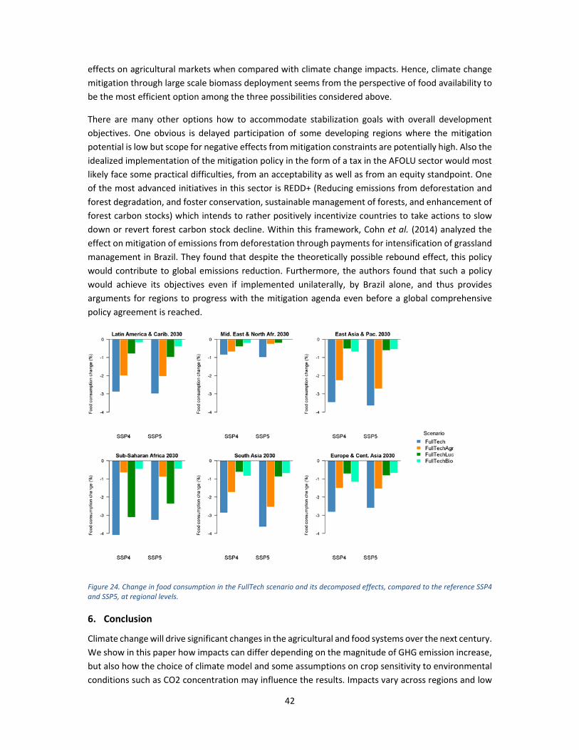
42  

effects on agricultural markets when compared with climate change impacts. Hence, climate change 

mitigation through large scale biomass deployment seems from the perspective of food availability to 

be the most efficient option among the three possibilities considered above. 

There  are many other options how  to  accommodate  stabilization  goals with overall development 

objectives. One obvious  is delayed participation of  some developing  regions where  the mitigation 

potential is low but scope for negative effects from mitigation constraints are potentially high. Also the 

idealized implementation of the mitigation policy in the form of a tax in the AFOLU sector would most 

likely face some practical difficulties, from an acceptability as well as from an equity standpoint. One 

of the most advanced initiatives in this sector is REDD+ (Reducing emissions from deforestation and 

forest degradation, and foster conservation, sustainable management of forests, and enhancement of 

forest carbon stocks) which  intends to rather positively  incentivize countries to take actions to slow 

down or revert forest carbon stock decline. Within this framework, Cohn et al. (2014) analyzed the 

effect on mitigation of emissions from deforestation through payments for intensification of grassland 

management in Brazil. They found that despite the theoretically possible rebound effect, this policy 

would contribute to global emissions  reduction. Furthermore, the authors  found that such a policy 

would  achieve  its  objectives  even  if  implemented  unilaterally,  by  Brazil  alone,  and  thus  provides 

arguments  for regions to progress with the mitigation agenda even before a global comprehensive 

policy agreement is reached. 

 

Figure 24. Change in food consumption in the FullTech scenario and its decomposed effects, compared to the reference SSP4 and SSP5, at regional levels. 

6. Conclusion 

Climate change will drive significant changes in the agricultural and food systems over the next century. 

We show in this paper how impacts can differ depending on the magnitude of GHG emission increase, 

but also how the choice of climate model and some assumptions on crop sensitivity to environmental 

conditions such as CO2 concentration may influence the results. Impacts vary across regions and low 

43  

income  countries  are  relatively more  affected  than  some other  regions due  to  their  geographical 

location, and to the higher vulnerability of their food consumer to change in agricultural prices. 

The agriculture and forestry sectors will likely be increasingly asked to contribute to mitigation efforts 

as well. This participation to achieve GHG reductions could present opportunities for land use sectors, 

with new demand for biomass, potential payments for carbon sequestration and higher margins for 

producers. However, mitigation policies could also bring significant challenges, because production 

costs will also increase with expansion of the production, and the deployment of new technologies will 

require  some  significant  restructuring of  the  sectors. More worrying,  the  consumers will be more 

directly affected by the increased market prices, with potential challenges for food security. 

Comparing the climate change impacts on food availability with the effects of mitigation, if mitigation 

is not implemented carefully, it could potentially bring worse effects for food availability than climate 

change itself, at least in the medium term. Hence, a careful design of mitigation policies needs to be 

adopted  by  targeting  priority  sectors  and  sources where  emission  abatement  can  be  achieved  at 

lowest  costs, without  hampering  food  provision.  The  contribution  of  the  poorest  regions  to  such 

scheme should be envisaged prudently, in order to avoid a double burden for people already facing 

the most  severe  climate  change  impact  challenges.  On  the  other  side,  the  carbon  tax  revenue 

represents a potentially substantial source of new fiscal income, which if managed properly, could be 

used  for  funding  of  direct  development  programs  and  hence  converted  from  a  thread  to  an 

opportunity for the poor. 

This study presents a first attempt to provide consistent quantitative assessment of climate change 

impacts and mitigation in agriculture and forestry on markets and food availability in low and medium 

income countries. Future improvements could go in several directions. For instance, we have ignored 

the combined effects of climate change and mitigation. We are convinced that this remains a second 

order  effect  of  the  extreme  climate  scenarios  considered  by  the  present  paper,  however  if 

intermediate scenarios such as RCP4.5 and RCP6.0 with non‐negligible aspects of both climate change 

impacts  and mitigation were  to  be  considered,  the  two  phenomenon might  represent  important 

feedbacks; e.g. climate change impacts reducing biomass productivity and hence making the provision 

of the bioenergy sector more expensive versus afforestation occupying vast areas of land making it not 

available for crop area expansion to moderate the negative climate impacts.  

To  conclude,  the projected  effects of  climate  change  and mitigation on  agricultural markets  raise 

important issues for food security in the long run, but remain more limited in the medium term horizon 

of  2030,  providing  opportunities  for  low‐  and  middle‐income  countries  to  pursue  immediate 

development needs and thus prepare for later periods when adaptation needs and mitigation efforts 

will become the greatest. 

 

 

References 

Alexandratos, N., Bruinsma, J., 2012. World Agriculture Towards 2030/2050: The 2012 Revision. Food 

and Agriculture Organization of the United Nations, Rome. 

44  

Andrews, T., Gregory, J.M., Webb, M.J., Taylor, K.E., 2012. Forcing, feedbacks and climate sensitivity in 

CMIP5 coupled atmosphere‐ocean climate models. Geophysical Research Letters 39, n/a‐n/a. 

Beach, R.H., DeAngelo, B.J., Rose, S.K., Li, C., Salas, W., DelGrosso, S.J., 2008. Mitigation potential and 

costs for global agricultural greenhouse gas emissions. Agricultural Economics 38, 109‐115. 

Böttcher, H., Frank, S., Havlík, P., Elbersen, B., 2013. Future GHG emissions more efficiently controlled 

by  land‐use  policies  than  by  bioenergy  sustainability  criteria.  Biofuels,  Bioproducts  and 

Biorefining 7, 115‐125. 

Burney, J.A., Davis, S.J., Lobell, D.B., 2010. Greenhouse gas mitigation by agricultural intensification. 

Proceedings of the National Academy of Sciences 107, 12052‐12057. 

Cohn, A.S., Mosnier, A., Havlík, P., Valin, H., Herrero, M., Schmid, E., O’Hare, M., Obersteiner, M., 2014. 

Cattle ranching intensification in Brazil can reduce global greenhouse gas emissions by sparing 

land from deforestation. Proceedings of the National Academy of Sciences 111, 7236‐7241. 

Collins, M., Knutti, R., Arblaster, J., Dufresne, J.‐L., Fichefet, T., Friedlingstein, P., Gao, X., Gutowski, 

W.J., Johns, T., Krinner, G., Shongwe, M., Tebaldi, C., Weaver, A.J., Wehner, M., 2013. Long‐

term Climate Change: Projections, Commitments and Irreversibility. In: Stocker, T.F., Qin, D., 

Plattner, G.K., Tignor, M., Allen, S.K., Boschung, J., Nauels, A., Xia, Y., Bex, V., Midgley, P.M. 

(Eds.), Climate Change 2013: The Physical Science Basis. Contribution of Working Group I to 

the Fifth Assessment Report of the  Intergovernmental Panel on Climate Change. Cambridge 

University Press, Cambridge, United Kingdom and New York, NY, USA, pp. 1029‐1136. 

Cramer, W., Kicklighter, D.W., Bondeau, A., Iii, B.M., Churkina, G., Nemry, B., Ruimy, A., Schloss, A.L., 

Intercomparison, T.P.O.T.P.N.M., 1999. Comparing global models of  terrestrial net primary 

productivity (NPP): overview and key results. Global Change Biology 5, 1‐15. 

de Vries, M., de Boer, I.J.M., 2010. Comparing environmental impacts for livestock products: A review 

of life cycle assessments. Livestock Science 128, 1 ‐ 11. 

Frank, S., Böttcher, H., Havlík, P., Valin, H., Mosnier, A., Obersteiner, M., Schmid, E., Elbersen, B., 2013. 

How effective are the sustainability criteria accompanying the European Union 2020 biofuel 

targets? GCB Bioenergy 5, 306‐314. 

Friedlingstein, P., Meinshausen, M., Arora, V.K., Jones, C.D., Anav, A., Liddicoat, S.K., Knutti, R., 2014. 

Uncertainties in CMIP5 climate projections due to carbon cycle feedbacks. Journal of Climate 

27, 511‐526. 

Geist, H.J., Lambin, E.F., 2002. Proximate causes and underlying driving forces of tropical deforestation. 

BioScience 52, 143‐150. 

Gibbs, H.K., Ruesch, A.S., Achard, F., Clayton, M.K., Holmgren, P., Ramankutty, N., Foley, J.A., 2010. 

Tropical  forests were  the primary sources of new agricultural  land  in the 1980s and 1990s. 

Proceedings of the National Academy of Sciences 107, 16732‐16737. 

Havlík, P., Leclère, D., Valin, H., Herrero, M., Schmid, E., Soussana, J.‐F., Müller, C., Obersteiner, M., 

2015. Global climate change,  food supply and  livestock production systems: A bioeconomic 

analysis.  In:  Elbehri,  A.  (Ed.),  Climate  change  and  food  systems:  global  assessments  and 

implications for food security and trade. Food Agriculture Organization of the United Nations 

(FAO), Rome. 

45  

Havlík,  P.,  Schneider,  U.A.,  Schmid,  E.,  Böttcher,  H.,  Fritz,  S.,  Skalský,  R.,  Aoki,  K.,  De  Cara,  S., 

Kindermann, G., Kraxner, F., Leduc, S., McCallum,  I., Mosnier, A., Sauer, T., Obersteiner, M., 

2011. Global land‐use implications of first and second generation biofuel targets. Energy Policy 

39, 5690‐5702. 

Havlík, P., Valin, H., Herrero, M., Obersteiner, M., Schmid, E., Rufino, M.C., Mosnier, A., Thornton, P.K., 

Böttcher, H., Conant, R.T., Frank, S., Fritz, S., Fuss, S., Kraxner, F., Notenbaert, A., 2014. Climate 

change mitigation through livestock system transitions. Proceedings of the National Academy 

of Sciences 111, 3709‐3714. 

Havlík, P., Valin, H., Mosnier, A., Obersteiner, M., Baker, J.S., Herrero, M., Rufino, M.C., Schmid, E., 

2013. Crop Productivity and the Global Livestock Sector: Implications for Land Use Change and 

Greenhouse Gas Emissions. American Journal of Agricultural Economics 95, 442‐448. 

Herrero, M., Havlík, P., McIntire, J., Palazzo, A., Valin, H., 2014. African Livestock Futures: Realizing the 

potential of livestock for food security, poverty reduction and the environment in Sub‐Saharan 

Africa. Office of the Special Representative of the UN Secretary General for Food Security and 

Nutrition and the United Nations System Influenza Coordination. 

Herrero, M., Havlík, P., Valin, H., Notenbaert, A., Rufino, M.C., Thornton, P.K., Blümmel, M., Weiss, F., 

Grace, D., Obersteiner, M., 2013. Biomass use, production, feed efficiencies, and greenhouse 

gas emissions from global livestock systems. Proceedings of the National Academy of Sciences 

110, 20888‐20893. 

Hristov, A.N., Oh, J., Lee, C., Meinen, R., Montes, F., Ott, T., Firkins, J., Rotz, A., Dell, C., Adesogan, A., 

Yang, W., Tricarico, J., Kebreab, E., Waghorn, G., Dijkstra, J., Oosting, S., 2013. Mitigation of 

greenhouse gas emissions in livestock production – A review of technical options for non‐CO2 

emissions. Food and Agriculture Organization of the United Nations, Rome, Italy. 

IIASA, 2015. SSP Database v1. 

IPCC, 2013. Climate Change 2013: The Physical Science Basis. Contribution of Working Group I to the 

Fifth  Assessment  Report  of  the  Intergovernmental  Panel  on  Climate  Change.  Cambridge 

University Press, Cambridge, United Kingdom and New York, NY, USA. 

IPCC, 2014a. Climate Change 2014: Impacts, Adaptation, and Vulnerability. Part A: Global and Sectoral 

Aspects.  Contribution  of  Working  Group  II  to  the  Fifth  Assessment  Report  of  the 

Intergovernmental Panel on Climate Change. Cambridge University Press, Cambridge, United 

Kingdom and New York, NY, USA. 

IPCC, 2014b. Climate Change 2014: Mitigation of Climate Change. Contribution of Working Group III to 

the Fifth Assessment Report of the  Intergovernmental Panel on Climate Change. Cambridge 

University Press, Cambridge, United Kingdom and New York, NY, USA. 

Kindermann,  G.,  Obersteiner,  M.,  Sohngen,  B.,  Sathaye,  J.,  Andrasko,  K.,  Rametsteiner,  E., 

Schlamadinger, B., Wunder, S., Beach, R.H., 2008a. Global cost estimates of reducing carbon 

emissions through avoided deforestation. Proceedings of the National Academy of Sciences 

105, 10302. 

Kindermann,  G.E., McCallum,  I.,  Fritz,  S.,  Obersteiner, M.,  2008b.  A  global  forest  growing  stock, 

biomass and carbon map based on FAO statistics. Silva Fennica 42, 387. 

46  

Kriegler, E., Weyant, J., Blanford, G., Krey, V., Clarke, L., Edmonds, J., Fawcett, A., Luderer, G., Riahi, K., 

Richels, R., Rose, S., Tavoni, M., van Vuuren, D., 2014. The role of technology  for achieving 

climate policy objectives: overview of  the EMF 27  study on global  technology and  climate 

policy strategies. Climatic Change 123, 353‐367. 

Lauri, P., Havlík, P., Kindermann, G., Forsell, N., Böttcher, H., Obersteiner, M., 2014. Woody biomass 

energy potential in 2050. Energy Policy 66, 19 ‐ 31. 

Leclère, D., Havlík, P., Fuss, S., Schmid, E., Mosnier, A., Walsh, B., Valin, H., Herrero, M., Khabarov, N., 

Obersteiner,  M.,  2014.  Climate  change  induced  transformations  of  agricultural  systems: 

insights from a global model. Environmental Research Letters 9, 1748‐9326. 

Leclère,  D.,  Jayet,  P.‐A.,  De  Noblet‐Ducoudré,  N.,  2013.  Farm‐level  Autonomous  Adaptation  of 

European Agricultural Supply to Climate Change. Ecological Economics 87, 1–14. 

Lobell, D.B., Roberts, M.J., Schlenker, W., Braun, N., Little, B.B., Rejesus, R.M., Hammer, G.L., 2014. 

Greater Sensitivity to Drought Accompanies Maize Yield Increase in the U.S. Midwest. Science 

344, 516‐519. 

Lobell, D.B., Schlenker, W., Costa‐Roberts, J., 2011. Climate Trends and Global Crop Production Since 

1980. Science 333, 616‐620. 

Lotze‐Campen, H., von Lampe, M., Kyle, P., Fujimori, S., Havlik, P., van Meijl, H., Hasegawa, T., Popp, 

A., Schmitz, C., Tabeau, A., Valin, H., Willenbockel, D., Wise, M., 2014.  Impacts of  increased 

bioenergy  demand  on  global  food markets:  an  AgMIP  economic model  intercomparison. 

Agricultural Economics 45, 103‐116. 

Lutz, W., Butz, W.P., KC, S., 2014. World Population & Human Capital in the Twenty‐first Century. IIASA, 

Laxenburg, Austria. 

McCarl, B.A., Spreen, T.H., 1980. Price Endogenous Mathematical Programming as a Tool for Sector 

Analysis. American Journal of Agricultural Economics 62, 87‐102. 

McCollum, D., Krey, V., Kolp, P., Nagai, Y., Riahi, K., 2014. Transport electrification: A key element for 

energy system transformation and climate stabilization. Climatic Change 123, 651‐664. 

Mosnier, A., Havlík, P., Obersteiner, M., Aoki, K., Schmid, E., Fritz, S., McCallum,  I., Leduc, S., 2012. 

Modeling Impact of Development Trajectories and a Global Agreement on Reducing Emissions 

from Deforestation on Congo Basin Forests by 2030. Environmental and Resource Economics, 

1‐21. 

Mosnier, A., Obersteiner, M., Havlík, P., Schmid, E., Khabarov, N., Westphal, M., Valin, H., Frank, S., 

Albrecht, F., 2014. Global food markets, trade and the cost of climate change adaptation. Food 

Security 6, 29‐44. 

Müller, C., Robertson, R.D., 2014. Projecting future crop productivity for global economic modeling. 

Agricultural Economics 45, 37‐50. 

Myers, S.S., Zanobetti, A., Kloog, I., Huybers, P., Leakey, A.D., Bloom, A.J., Carlisle, E., Dietterich, L.H., 

Fitzgerald, G., Hasegawa, T., others, 2014. Increasing CO2 threatens human nutrition. Nature 

510, 139‐142. 

Nelson, G.C., 2009. Climate change:  Impact on agriculture and costs of adaptation.  Intl Food Policy 

Research Inst. 

47  

Nelson,  G.C.,  Valin,  H.,  Sands,  R.D.,  Havlík,  P.,  Ahammad,  H.,  Deryng,  D.,  Elliott,  J.,  Fujimori,  S., 

Hasegawa, T., Heyhoe, E., Kyle, P., von Lampe, M., Lotze‐Campen, H., Mason D'Croz, D., van 

Meijl, H., van der Mensbrugghe, D., Müller, C., Popp, A., Robertson, R., Robinson, S., Schmid, 

E.,  Schmitz,  C.,  Tabeau,  A., Willenbockel, D.,  2014.  Climate  change  effects  on  agriculture: 

Economic responses to biophysical shocks. Proceedings of the National Academy of Sciences 

111, 3274‐3279. 

O’Neill, B., Kriegler, E., Riahi, K., Ebi, K., Hallegatte, S., Carter, T., Mathur, R., Vuuren, D., 2014. A new 

scenario  framework  for  climate  change  research:  the  concept  of  shared  socioeconomic 

pathways. Climatic Change 122, 387‐400. 

Obersteiner, M.,  Azar,  C.,  Kauppi,  P., Möllersten,  K., Moreira,  J.,  Nilsson,  S.,  Read,  P.,  Riahi,  K., 

Schlamadinger, B., Yamagata, Y., others, 2001. Managing climate risk. Science 294, 786‐787. 

Osborne, T., Rose, G., Wheeler, T., 2013. Variation  in the global‐scale  impacts of climate change on 

crop productivity due to climate model uncertainty and adaptation. Agricultural and Forest 

Meteorology 170, 183–194. 

Peters, G.P., Andrew, R.M., Boden, T., Canadell, J.G., Ciais, P., Le Quere, C., Marland, G., Raupach, M.R., 

Wilson, C., 2013. The challenge to keep global warming below 2 [deg]C. Nature Clim. Change 

3, 4‐6. 

Popp, A., Lotze‐Campen, H., Bodirsky, B., 2010. Food consumption, diet shifts and associated non‐CO2 

greenhouse gases from agricultural production. Global Environmental Change 20, 451‐462. 

Porter, J.R., Xie, L., Challinor, A.J., Cochrane, K., Howden, S.M., Iqbal, M.M., Lobell, D.B., Travasso, M.I., 

2014. Food security and  food production systems.  In: Field, C.B., Barros, V.R., Dokken, D.J., 

Mach, K.J., Mastrandrea, M.D., Bilir, T.E., Chatterjee, M., Ebi, K.L., Estrada, Y.O., Genova, R.C., 

Girma, B., Kissel, E.S., Levy, A.N., MacCracken, S., Mastrandrea, P.R., White, L.L. (Eds.), Climate 

Change 2014:  Impacts, Adaptation,  and Vulnerability. Part A: Global  and  Sectoral Aspects. 

Contribution of Working Group  II  to  the Fifth Assessment Report of  the  Intergovernmental 

Panel of Climate Change. Cambridge University Press, Cambridge, United Kingdom and New 

York, NY, USA, pp. 485‐533‐. 

Reilly, J., Melillo, J., Cai, Y., Kicklighter, D., Gurgel, A., Paltsev, S., Cronin, T., Sokolov, A., Schlosser, A., 

2012. Using  land  to mitigate  climate  change: hitting  the  target,  recognizing  the  trade‐offs. 

Environmental science & technology 46, 5672‐5679. 

Reisinger,  A.,  Havlík,  P.,  Riahi,  K.,  Vliet,  O.,  Obersteiner, M.,  Herrero, M.,  2012.  Implications  of 

alternative metrics for global mitigation costs and greenhouse gas emissions from agriculture. 

Climatic Change, 1‐14. 

Rogelj, J., Meinshausen, M., Knutti, R., 2012. Global warming under old and new scenarios using IPCC 

climate sensitivity range estimates. Nature Clim. Change 2, 248‐253. 

Rose, S.K., Ahammad, H., Eickhout, B., Fisher, B., Kurosawa, A., Rao, S., Riahi, K., van Vuuren, D.P., 

2012. Land‐based mitigation in climate stabilization. Energy Economics, 365‐‐380. 

Rosenzweig, C., Elliott,  J., Deryng, D., Ruane, A.C., Müller, C., Arneth, A., Boote, K.J.,  Folberth, C., 

Glotter, M., Khabarov, N., Neumann, K., Piontek, F., Pugh, T.A.M., Schmid, E., Stehfest, E., Yang, 

H.,  Jones,  J.W., 2014. Assessing agricultural risks of climate change  in the 21st century  in a 

48  

global gridded crop model intercomparison. Proceedings of the National Academy of Sciences 

111, 3268‐3273. 

Smith, P., Bustamante, M., Ahammad, H., Clark, H., Don, H., Elsiddig, E.A., Haberl, H., Harper, R., House, 

J., Jafari, M., Masera, O., Mbow, C., Ravindranath, N.H., Rice, C.W., Aba, C.R., Romanovskaya, 

A., Sperling, F., Tubiello, F., 2014. Agriculture, Forestry and Other Land Use (AFOLU). Climate 

Change 2014: Mitigation of Climate Change. Contribution of Working Group  III  to  the Fifth 

Assessment Report of the Intergovernmental Panel on Climate Change. Edenhofer, O., R. Pichs‐

Madruga,  Y.  Sokona,  E.  Farahani,  S.  Kadner,  K.  Seyboth,  A. Adler,  I.  Baum,  S.  Brunner,  P. 

Eickemeier, B. Kriemann, J. Savolainen, S. Schlömer, C. von Stechow, T. Zwickel and J.C. Minx, 

Cambridge, United Kingdom and New York, NY, USA. 

Smith, P., Martino, D., Cai, Z., Gwary, D., Janzen, H., Kumar, P., McCarl, B., Ogle, S., O'Mara, F., Rice, 

C.W.,  Scholes,  B.,  Sirotenko,  O.,  Howden,  M.,  McAllister,  T.,  Pan,  G.,  Romanenkov,  V., 

Schneider, U., Towprayoon, S., Wattenbach, M., Smith, J., 2008. Greenhouse gas mitigation in 

agriculture. Philosophical Transactions of the Royal Society B: Biological Sciences 363, 789‐813. 

Stehfest, E., Bouwman, A.F., van Vuuren, D.P., den Elzen, M., Eickhout, B., Kabat, P., 2009. Climate 

benefits of changing diet. Climatic Change 95, 83‐102. 

Takayama, T.,  Judge, G.G., 1971.  Spatial  and  temporal price  and allocation models. North‐Holland 

Amsterdam. 

Taylor,  K.E.,  Stouffer,  R.J., Meehl, G.A.,  2011. An Overview  of  CMIP5  and  the  Experiment Design. 

Bulletin of the American Meteorological Society 93, 485‐498. 

Thornton, P.K., van de Steeg, J., Notenbaert, A., Herrero, M., 2009. The impacts of climate change on 

livestock and livestock systems in developing countries: A review of what we know and what 

we need to know. Agricultural Systems 101, 113‐127. 

Tubiello, F.N., Amthor, J.S., Boote, K.J., Donatelli, M., Easterling, W., Fischer, G., Gifford, R.M., Howden, 

M., Reilly, J., Rosenzweig, C., 2007. Crop response to elevated CO2} and world food supply: A 

comment on “Food  for Thought…” by Long et al., Science 312:1918–1921, 2006. European 

Journal of Agronomy 26, 215 ‐ 223. 

Valin,  H.,  Havlík,  P.,  Mosnier,  A.,  Herrero,  M.,  Schmid,  E.,  Obersteiner,  M.,  2013.  Agricultural 

productivity and greenhouse gas emissions: trade‐offs or synergies between mitigation and 

food security? Environmental Research Letters 8, 035019. 

Valin, H., Sands, R.D., van der Mensbrugghe, D., Nelson, G.C., Ahammad, H., Blanc, E., Bodirsky, B., 

Fujimori,  S., Hasegawa,  T., Havlík,  P., Heyhoe,  E.,  Kyle,  P., Manson‐D'Croz, D.,  Paltsev,  S., 

Rolinski, S., Tabeau, A., van Meijl, H., von Lampe, M., Willenbockel, D., 2014. The Future of 

Food Demand: Understanding Differences in Global Economic Models. Agricultural Economics 

45, 51‐67. 

van Vuuren, D., Kriegler, E., O’Neill, B., Ebi, K., Riahi, K., Carter, T., Edmonds, J., Hallegatte, S., Kram, T., 

Mathur,  R., Winkler,  H.,  2014.  A  new  scenario  framework  for  Climate  Change  Research: 

scenario matrix architecture. Climatic Change 122, 373‐386. 

van Vuuren, D.P., Edmonds, J., Kainuma, M., Riahi, K., Thomson, A., Hibbard, K., Hurtt, G.C., Kram, T., 

Krey, V., Lamarque, J.‐F., Masui, T., Meinshausen, M., Nakicenovic, N., Smith, S., Rose, S.K., 

2011. The representative concentration pathways: an overview. Climatic Change 109, 5‐31. 

49  

Vial, J., Dufresne, J.‐L., Bony, S., 2013. On the interpretation of inter‐model spread in CMIP5 climate 

sensitivity estimates. Climate Dynamics 41, 3339‐3362. 

von Lampe, M., Willenbockel, D., Ahammad, H., Blanc, E., Cai, Y., Calvin, K., Fujimori, S., Hasegawa, T., 

Havlík, P., Heyhoe, E., Kyle, P., Lotze‐Campen, H., Mason D.'Croz, D., Nelson, G.C., Sands, R.D., 

Schmitz, C., Tabeau, A., Valin, H., van der Mensbrugghe, D., van Meijl, H., 2014. Why do global 

long‐term scenarios for agriculture differ? An overview of the AgMIP Global Economic Model 

Intercomparison. Agricultural Economics 45, 3‐20. 

Warszawski, L., Frieler, K., Huber, V., Piontek, F., Serdeczny, O., Schewe, J., 2013. The Inter‐Sectoral 

Impact Model  Intercomparison  Project  (ISI–MIP):  Project  framework.  Proceedings  of  the 

National Academy of Sciences. 

Williams, J.R., 1995. The EPIC model. In: Singh, V.P. (Ed.). Water Resources Publications, pp. 909‐1000. 

Wise, M., Calvin, K., Thomson, A., Clarke, L., Bond‐Lamberty, B., Sands, R.D., Smith, S.J., Janetos, A., 

Edmonds,  J.,  2009.  Implications  of  Limiting  CO2  Concentrations  for  Land Use  and  Energy. 

Science 324, 1183‐1186. 

Zekarias, H., Thomas, H., Alla, G., 2013. Climate change mitigation policies and poverty in developing 

countries. Environmental Research Letters 8, 035009. 

 

   

50  

Appendices 

A. List of crops used in the paper 

Table‐A 1. List of crop codes used in GLOBIOM 

CODE  NAME 

WHEA  Wheat 

RICE  Rice 

CORN  Corn 

SOYA  Soybean 

RAPE  Rapeseed 

BARL  Barley 

CASS  Cassava 

SUNF  Sunflower 

MILL  Millet 

SRGH  Sorghum 

SUGC  Sugar cane 

BEAD  Dry beans 

COTT  Cottonseed 

CHKP  Chick peas 

SWPO  Sweet potatoes 

POTA  Potatoes 

GNUT  Groundnuts 

OPAL  Oil palm fruit 

 

   

51  

B.  Regional grouping 

Table‐A 2. List of regions used in the paper, mapping with GLOBIOM regions and corresponding countries 

Macro region  GLOBIOM regions 

Countries 

West Europe  EU Baltic  Estonia, Latvia, Lithuania 

EU Central East  Bulgaria, Czech Republic, Hungary, Poland, Romania, Slovakia, Slovenia 

EU Mid West  Austria, Belgium, Germany, France, Luxembourg, Netherlands 

EU North  Denmark, Finland, Ireland, Sweden, United Kingdom 

EU South  Cyprus, Greece, Italy, Malta, Portugal, Spain 

ROWE  Gibraltar, Iceland, Norway, Switzerland 

Eastern Europe and Central Asia 

Former USSR  Armenia,  Azerbaijan,  Belarus,  Georgia,  Kazakhstan,  Kyrgyzstan,  Moldova, Russian Federation, Tajikistan, Turkmenistan, Ukraine, Uzbekistan 

Turkey  Turkey 

RCEU  Albania, Bosnia and Herzegovina, Croatia, Macedonia, Serbia‐Montenegro 

North America  Canada  Canada 

United States  United States 

Latin America and the Caribbean 

Brazil  Brazil 

Mexico  Mexico 

RCAM  Bahamas, Barbados, Belize, Bermuda, Costa Rica, Cuba, Dominica, Dominican Republic, El Salvador, Grenada, Guatemala, Haiti, Honduras, Jamaica, Nicaragua, Netherland Antilles, Panama, St Lucia, St Vincent, Trinidad and Tobago 

RSAM  Argentina, Bolivia, Chile, Colombia, Ecuador, Guyana, Paraguay, Peru, Suriname, Uruguay, Venezuela, RB 

Eastern  Asia  and Pacific 

China  China 

RSEA OPA  Brunei  Daressalaam,  Indonesia,  Singapore,  Malaysia,  Myanmar,  Philippines, Thailand 

RSEA PAC  Cambodia; Korea, Dem. People’s Rep.; Lao PDR; Mongolia; Vietnam 

Pacific Islands  Fiji Islands, Kiribati, Papua New Guinea, Samoa, Solomon Islands, Tonga, Vanuatu 

Pacific Developed 

ANZ  Australia, New Zealand 

Japan  Japan 

Korea, Rep.  Korea, Rep. 

South Asia  India  India 

RSAS  Afghanistan, Bangladesh, Bhutan, Maldives, Nepal, Pakistan, Sri Lanka 

Middle‐East  and North Africa 

Middle East and North Africa  

Algeria, Bahrain, Egypt, Arab Rep., Iran, Islamic Rep., Iraq, Israel, Jordan, Kuwait, Lebanon,  Libya, Morocco,  Oman,  Qatar,  Saudi  Arabia,  Syrian  Arab  Republic, Tunisia, United Arab Emirates, Yemen, Rep. 

Sub‐Saharan Africa 

Congo Basin  Cameroon, Central African Republic, Congo, Rep., Congo, Dem. Rep., Equatorial Guinea, Gabon 

Eastern Africa  Burundi, Ethiopia, Kenya, Rwanda, Tanzania, Uganda 

South Africa    

Southern  Africa (Rest of) 

Angola,  Botswana,  Comoros,  Lesotho,  Madagascar,  Malawi,  Mauritius, Mozambique, Namibia, Swaziland, Zambia, Zimbabwe 

West and Central Africa 

Benin, Burkina Faso, Cape Verde, Chad, Côte d'Ivoire, Djibouti, Eritrea, Gambia, Ghana, Guinea, Guinea Bissau, Liberia, Mali, Mauritania, Niger, Nigeria, Senegal, Sierra Leone, Somalia, Sudan, Togo 

 

52  

C. List of scenarios 

The list of scenarios below has been used for this paper. These have been run under two 

macroeconomic context: SSP4 and SSP5. Therefore, 36 scenarios were in total analysed. 

Table‐A 3. Full list of scenarios used in the paper 

ID  GCM  CLIMATE CHANGE 

CLIMATE MITIGATION 

COMMENT 

B  None  No CC  None  Baseline 

 

C1  HadGEM2‐ES  RCP2.6  None  Climate scenario RCP2.6 with CO2 effects 

C2  IPSL‐CM5A‐LR  RCP2.6  None  Climate scenario RCP2.6 with CO2 effects 

C3  GFDL‐ESM2M  RCP2.6  None  Climate scenario RCP2.6 with CO2 effects 

C4  MIROC‐ESM‐CHEM 

RCP2.6  None  Climate scenario RCP2.6 with CO2 effects 

C5  NorESM1‐M  RCP2.6  None  Climate scenario RCP2.6 with CO2 effects 

C6  HadGEM2‐ES  RCP8.5  None  Climate scenario RCP8.5 with CO2 effects 

C7  IPSL‐CM5A‐LR  RCP8.5  None  Climate scenario RCP8.5 with CO2 effects 

C8  GFDL‐ESM2M  RCP8.5  None  Climate scenario RCP8.5 with CO2 effects 

C9  MIROC‐ESM‐CHEM 

RCP8.5  None  Climate scenario RCP8.5 with CO2 effects 

C10  NorESM1‐M  RCP8.5  None  Climate scenario RCP8.5 with CO2 effects 

C11  HadGEM2‐ES  RCP8.5*  None  Climate scenario RCP8.5 without CO2 effects 

CX1  Avg  RCP2.6  None  Average over GCMs RCP2.6 with CO2 effects 

CX2  Avg  RCP8.5  None  Average over GCMs RCP8.5 with CO2 effects 

CX3  Avg  RCP8.5*  None  Average over GCMs RCP8.5 without CO2 effects (equal to C11) 

 

M1  None  No CC  FullTech  Mitigation policy 2 degrees ‐ high energy intensity world ‐ high biomass use  

M2  None  No CC  LowEI  Mitigation policy 2 degrees ‐ low energy intensity world ‐ high biomass use 

M3  None  No CC  LimBio  Mitigation policy 2 degrees ‐ limited biomass use 

M1A  None  No CC  FullTechAgr  Mitigation policy 2 degrees ‐ M1 ‐ carbon tax on agriculture only 

M1B  None  No CC  FullTechLUC  Mitigation policy 2 degrees ‐ M1 ‐ carbon tax on land use emissions only 

M1C  None  No CC  FullTechBio  Mitigation policy 2 degrees ‐ M1 ‐ bioenergy expansion only 

 

   

53  

D. Complementary figures 

 

Figure D‐1. Climate change impact on average crop yield for six regions in 2030 for different climate scenarios and climate models. Crops correspond to the 18 species represented in GLOBIOM and are aggregated on a dry matter yield basis. 

 

Figure D‐2. Climate change impact on by crop for six regions in 2030 for the RCP 8.5 scenario with CO2 effects. Impacts are averaged across the five GCMs in the analysis. Only crops with cultivated areas greater than 100,000 ha in 2000 are represented. Crop acronyms:  WHEA= wheat, RICE = rice, CORN = corn, SOYA = soybean, RAPE = rapeseed, BARL = barley, CASS = cassava, SUNF = sunflower, MILL = millet, SRGH = sorghum, SUGC = sugar cane, BEAD = dry beans, COTT = cottonseed, CHKP = chick peas, SWPO = sweet potatoes, POTA = potatoes, GNUT = groundnuts. 

54  

 

 

Figure D‐3. Propagation of climate change impact along the chain of economic indicators for SSP4 and SSP5 in 2030 for RCP 8.5 with CO2 effects. CC shock corresponds to the average biophysical impact of climate change on dry matter yield; Yield corresponds to final resulting dry matter yield, including adaptation response; Area is the total change in harvested area; Prod is the change in total crop production in dry matter basis; Price is the average crop price index; Trade sh. corresponds to difference in the share of interregional trade (export – import) in total crop production; conso is the change in total crop consumption, and food and feed the relative change in the consumption of food and feed.  Units are relative change to the baseline.