climate change adaptation: perspectives on food … change adaptation: perspectives on ... white...
TRANSCRIPT

i
Climate Change Adaptation: Perspectives
on Food Security in South Africa
Towards an Integrated Economic Analysis
REPORT No. 5 FOR THE
LONG TERM ADAPTATION SCENARIOS FLAGSHIP RESEARCH PROGRAM (LTAS)

ii
Table of Contents
Executive summary ............................................................................................................................... vii
1 Introduction .................................................................................................................................... 1
2 Methodology ................................................................................................................................... 4
2.1 The sector model .................................................................................................................... 4
2.2 Consumer Impact study .......................................................................................................... 5
2.3 Climate Data ............................................................................................................................ 7
3 Climate Change Impacts on Production and Prices ........................................................................ 9
3.1 Developing the LTAS BASE 2030 projections .......................................................................... 9
3.2 Comparing the LTAS scenarios to the base ........................................................................... 17
3.2.1 Maize ............................................................................................................................. 17
3.2.2 Wheat ............................................................................................................................ 20
4 Consumer Impact Study ................................................................................................................ 23
4.1 Approach 1: The ‘BFAP Poor person’s index ......................................................................... 23
4.2 Approach 2: Staple food expenditure pattern based analysis .............................................. 25
4.2.1 Annual household food expenditure implications ........................................................ 25
4.2.2 Energy intake implications of an constrained food budget .......................................... 25
4.3 Conclusion: ............................................................................................................................ 26
5 Climate Change Impacts on Agricultural Employment ................................................................. 26
6 Food security and adaptation responses ...................................................................................... 29
6.1 Small scale agriculture and food security ............................................................................. 29
6.2 Continual adaptation and technology .................................................................................. 31
6.3 Irrigation ................................................................................................................................ 32
6.4 Expansion of area planted .................................................................................................... 33
7 High-level messages and Policy recommendations ...................................................................... 34
8 Future research needs with links to future adaptation work and modelling capacity ................. 36
Annexes ................................................................................................................................................. 39

iii
List of figures Figure 1: The BFAP modelling system ..................................................................................................... 5
Figure 2: Rainfall for maize production: Historical and forecast .......................................................... 10
Figure 3: SA main field crop area .......................................................................................................... 11
Figure 4: Base - White maize production, consumption and yield ....................................................... 12
Figure 5: White maize price and trade space ....................................................................................... 13
Figure 6: Base - Yellow maize production, consumption and yield ...................................................... 13
Figure 7: Base Yellow maize price and trade space .............................................................................. 14
Figure 8: Base - Wheat production, consumption and yield ................................................................ 15
Figure 9: Base - Wheat price and trade space ...................................................................................... 15
Figure 10: South African Maize: Area Planted and Yield (5 year moving averages) ............................. 16
Figure 11: Precipitation influencing maize production– base versus alternative scenarios ................ 17
Figure 12: Base versus scenarios: white maize average yield .............................................................. 18
Figure 13: Base versus scenarios: white maize average SAFEX prices .................................................. 18
Figure 14: Stochastic precipitation – Base versus MPI 4.5 ................................................................... 19
Figure 15: Stochastic white maize price – Base versus MPI 4.5 ........................................................... 19
Figure 16: South African Wheat Production and Domestic Use ........................................................... 20
Figure 17: The BFAP Poor person’s index – Projected results .............................................................. 24
Figure 18: Cost share contributions of maize meal within the weighted five item food plate ............ 24
Figure 19: BFAP Employment matrix .................................................................................................... 27
Figure 20: Percentage Changes - Maize Employment .......................................................................... 28
Figure 21: Percentage Changes - Wheat Employment ......................................................................... 28
Figure 22: Reason for engaging in Agriculture ...................................................................................... 30
List of Tables Table 1: Yield effects (% change from 2000 to 2050) by crop and management system ...................... 1
Table 2: Price outcomes of the overall scenarios ................................................................................... 2
Table 3: Composition of the BFAP Poor person’s index ......................................................................... 6
Table 4: LTAS Scenario Representative Models (2040-2050) ................................................................. 8
Table 5: Macro-economic baseline assumptions .................................................................................... 9
Table 6: Poor person food basket cost and composition ..................................................................... 23
Table 7: Compounded annual growth rates in employment ................................................................ 28
Table 8: Household sources of income, 2010 ....................................................................................... 29
Table 9: South African households’ access to agricultural land, 2010.................................................. 30
Table 10: Agricultural irrigation: Area and Method .............................................................................. 33

iv
List of abbreviations
ACCESS Australian Community Climate and Earth-System Simulator
BFAP Bureau for Food and Agricultural Policy
CF Carbon Dioxide Fertilisation
CSIRO Commonwealth Scientific and Industrial Research Organization
DSSAT Decision Support System for Agrotechnology Transfer
FAO Food and Agricultural Organisation
FAPRI Food and Agricultural Policy Research Institute
IES Income and Expenditure Survey
IFPRI International Food Policy Research Institute
GAM Generalized Additive Models
IMPACT Model for Policy Analysis of Agricultural Commodities and Trade
IPCC Intergovernmental Panel on Climate Change
IPCC AR4 Intergovernmental Panel on Climate Change Fourth Assessment Report
IPCC AR5 Intergovernmental Panel on Climate Change Fifth Assessment Report
LTAS Long Term Adaptation Scenario’s
MPI Max Planck Institute for Meteorology
NAMC National Agricultural Marketing Council
NCAR National Centre for Atmospheric Research
NoCF No Carbon Dioxide Fertilisation
OECD Organisation for Economic Co‑operation and Development
RCP Representative Concentration Pathways
SAWIS South African Weather Information Service
StatsSA Statistics South Africa
UCS Union for Concerned Scientists
WAS Water Management System

v
Acknowledgements 1
2
The Long-Term Adaptation Flagship Research Programme (LTAS) responds to the South African 3
National Climate Change Response White Paper by undertaking climate change adaptation research 4
and scenario planning for South Africa and the Southern African sub-region. The Department of 5
Environmental Affairs (DEA) is leading the process in collaboration with technical research partner 6
the South African National Biodiversity Institute (SANBI) as well as technical and financial assistance 7
from the Gesellschaft für Internationale Zusammenarbeit (GIZ). 8
9
DEA would like to acknowledge the LTAS Phase 1 and 2 Project Management Team who contributed 10
to the development of the LTAS research and policy products, namely Mr Shonisani Munzhedzi, Mr 11
Vhalinavho Khavhagali (DEA), Prof Guy Midgley (SANBI), Ms Petra de Abreu, Ms Sarshen Scorgie 12
(Conservation South Africa), Dr Michaela Braun, and Mr Zane Abdul (GIZ). DEA would also like to 13
thank the sector departments and other partners for their insights to this work, in particular the 14
Department of Water Affairs (DWA), Department of Agriculture, Forestry and Fisheries (DAFF), 15
National Disaster Management Centre (NDMC), Department of Rural Development and Land Reform 16
(DRDLR), South African Weather Services (SAWS). 17
18
Specifically, we would like to extend gratitude to the groups, organisations and individuals who 19
compiled the “Climate Change Adaptation: Perspectives on Food Security in South Africa” report, 20
namely the Bureau for Food and Agricultural Policy (http://www.bfap.co.za), including Prof Ferdi 21
Meyer (University of Pretoria), Jan Greyling (University of Stellenbosch), Gerhard van der Burgh 22
(Bureau for Food and Agricultural Policy [BFAP] analyst), Hester Vermeulen (BFAP analyst), Marion 23
Muhl (University of Pretoria), and Dr Lindsay Trapnell (University of Pretoria); and Dr James Cullis 24
(Aurecon) who provided the rainfall data for the future scenarios analysed in this report. 25
Furthermore, we thank the stakeholders who attended the LTAS workshops for their feedback and 26
inputs on proposed methodologies, content and results. Their contributions were instrumental to 27
this final report. 28
29
Over the past decade Bureau for Food and Agricultural Policy (BFAP) (www.bfap.co.za) has become a 30
valuable resource to government, agribusiness and farmers by providing analyses of future policy 31
and market scenarios and measuring their impact on farm and firm profitability. BFAP is a network 32
linking individuals with multi-disciplinary backgrounds to a coordinated research system that informs 33
decision making within the Food System. The core analytical team consists of independent analysts 34
and researchers who are affiliated with the Department of Agricultural 35
Economics, Extension and Rural Development at the University of 36
Pretoria, the Department of Agricultural Economics at the University 37
of Stellenbosch, or the Directorate of Agricultural Economics at the 38
Provincial Department of Agriculture, Western Cape. BFAP 39
acknowledges and appreciates the tremendous insight of numerous 40
industry specialists over the past decade. 41

vi
Report overview 1
This report develops preliminary high level messages on the socio-economic and food security 2
impacts of climate change in South Africa, including consideration of impacts on South African 3
consumers and employment in the agricultural sector, and implications for adaptation. Findings are 4
preliminary because they are based on impacts only on the two main staple cereal crops only (maize 5
and wheat) of a limited set of downscaled LTAS climate scenarios. 6
7
The first objective of this study is to translate the selected climate scenarios into maize and wheat 8
production and price effects. In order to achieve this goal the results of four downscaled climate 9
models were incorporated into an econometric, recursive partial equilibrium model of the South 10
African agricultural sector. Within this model, rainfall, both in terms of the total during the 11
production season and the timing thereof, represent one of a host of variables that impact on the 12
eventual results on total area planted, total production and commodity price changes. These results 13
are compared to a baseline scenario that is generated from historic rainfall data. This study 14
therefore provides an economic perspective on the LTAS climate scenarios which bio-dynamic 15
modelling approaches are unable to do. The results also provide a simulated perspective on how 16
producers choose to respond to climate change in terms of area planted and the resulting impact on 17
the equilibrium of demand and supply in maize and wheat markets. 18
19
The second objective of this study is to incorporate these results into a consumer impact analysis in 20
order to evaluate the price effects of the respective climate scenarios on poor households. Within 21
this analysis three approaches where followed: The first is the ‘BFAP Poor person’s index’ is based on 22
the price of typical portion sizes of poor South African consumers’ typical portion sizes of the five 23
most widely consumed food items in South Africa. The second is the StatsSA Income and 24
Expenditure based analysis. The third is the balanced food plate approach that follows a balanced 25
daily food plate approach. 26
27
The third objective of this study is to evaluate the impact of these possible climate futures on 28
agricultural employment. This was achieved through incorporating the results into the BFAP 29
employment model. Collectively these results are interpreted in terms of their food security impacts, 30
both in terms of supply and access. This is translated into adaptation and mitigation 31
recommendations, policy recommendations and future research needed. 32
Chapter 1 (Introduction) provides an overview previous comparable research and will link with LTAS 33
phase 1, specifically the LTAS phase 1 report (no.3 of 6) on agriculture and forestry. 34
Chapter 2 & 3 (Methodology and Data) delivers an overview of the respective methodologies used in 35
the study and provide an overview of the data used within the relevant models. 36
Chapter 4 (Crop model results) provides the results of the partial equilibrium modelling in terms of 37
the changes in the area planted, total production, trade and price of maize and wheat due to the 38
respective climate scenarios. 39
Chapter 5 (Consumer Impact Study) presents the results of the consumer impact study. 40
Chapter 6 (Employment impacts) provides the results on the possible agricultural employment 41
impacts of the respective climate scenarios. 42
Chapter 7 (Food security and messages) this section concludes with a discussion of the food security 43
impacts, mitigation and adaptation responses, policy recommendations and future research needed. 44
45

vii
Executive summary 1
2
There have been numerous studies on the effects of potential climate change on crop suitability and 3
productivity from a Southern- and South African perspective. These studies, however, do not provide 4
an integrated perspective of how the agricultural and food system could be affected under various 5
climate change scenarios from an economic and social perspective. Therefore a key need is to 6
translate the respective climate scenarios into economic impacts, both in terms of the food access 7
(price) perspective of food security but also in terms of the impact on the decision to produce, which 8
impacts on agricultural employment. This study aims to fill this gap through a stochastic partial 9
equilibrium modelling approach in order to provide high level messages on the impact of climate 10
change on South African maize and wheat production towards 2030. 11
12
Within this study precipitation data generated from various climate models that best describe drying 13
LTAS climate scenarios were evaluated through the BFAP sector model. This sector model can be 14
best described as an econometric, recursive partial equilibrium model of the South African 15
agricultural sector, which presently covers 52 commodities. The results obtained were analysed 16
further from a consumer impact and employment perspective. The objective of this study is to 17
provide high level messages on the potential impact of climate change on food security and 18
employment under a set of assumptions in order to relate these into policy recommendations that 19
will enable adaptation and mitigation. This study has a strong element of foresighting and in order to 20
achieve these objectives, a combination of modelling tools is applied. When undertaking foresighting 21
analyses, it is useful to consider the future stochastic range of key fundamental variables and not 22
only be fixated on the deterministic projections. It is far more important to explore the possible 23
ranges of key variables and how climate change can potentially have an impact on the maize and 24
wheat industries. 25
26
For this study the actual precipitation data for the period 1950 to 2000 was modelled in order to 27
provide a “real world” baseline for 2000 to 2050 to which the results obtained from the inclusion of 28
the precipitation data from the various climate models could be compared. An analysis of the results 29
from the selected climate models only showed a significant divergence after 2030. In other words, it 30
is apparent that for most of the scenarios the effects on precipitation increase towards the end of 31
the simulation period only. Therefore, in order to analyse the potential economic impacts of climate 32
on the South African maize and wheat industries, the precipitation data projected for the period 33
2034 to 2050 is introduced into the BFAP sector model for each of the scenarios, which is then 34
compared to the base case. The BFAP sector model generates absolute and percentage shocks to 35
illustrate the relative deviations from the base. The implication thereof can be best described as the 36
effect of more than 20 years of climate change on the current context. It also became clear that only 37
one of the four climate models showed a significant deviation from the base after the data was 38
allocated according national maize and wheat production regions, both in terms of total 39
precipitation and the timing thereof. 40
41
An overview of the fundamental trends within the base precipitation scenario is essential for a 42
correct interpretation of the modelled results of the respective climate scenarios Under the base 43
scenario South Africa is anticipated to remain a net exporter of white and yellow maize (i.e. 44
domestic supply exceeds demand) and a net importer of wheat, with net imports growing beyond 45
viii
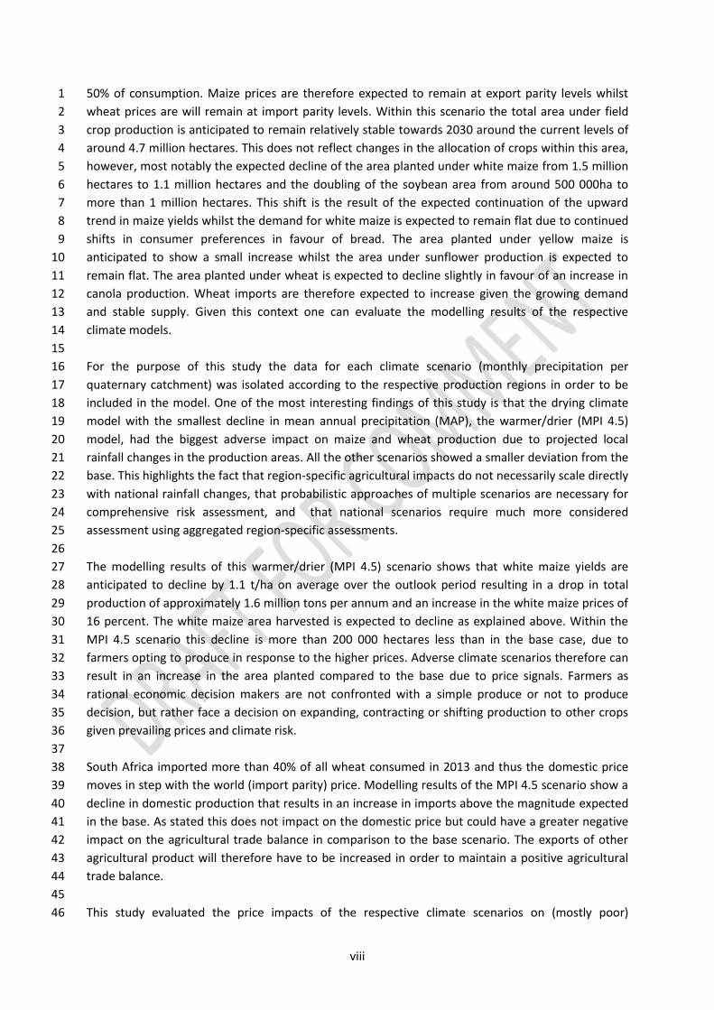
50% of consumption. Maize prices are therefore expected to remain at export parity levels whilst 1
wheat prices are will remain at import parity levels. Within this scenario the total area under field 2
crop production is anticipated to remain relatively stable towards 2030 around the current levels of 3
around 4.7 million hectares. This does not reflect changes in the allocation of crops within this area, 4
however, most notably the expected decline of the area planted under white maize from 1.5 million 5
hectares to 1.1 million hectares and the doubling of the soybean area from around 500 000ha to 6
more than 1 million hectares. This shift is the result of the expected continuation of the upward 7
trend in maize yields whilst the demand for white maize is expected to remain flat due to continued 8
shifts in consumer preferences in favour of bread. The area planted under yellow maize is 9
anticipated to show a small increase whilst the area under sunflower production is expected to 10
remain flat. The area planted under wheat is expected to decline slightly in favour of an increase in 11
canola production. Wheat imports are therefore expected to increase given the growing demand 12
and stable supply. Given this context one can evaluate the modelling results of the respective 13
climate models. 14
15
For the purpose of this study the data for each climate scenario (monthly precipitation per 16
quaternary catchment) was isolated according to the respective production regions in order to be 17
included in the model. One of the most interesting findings of this study is that the drying climate 18
model with the smallest decline in mean annual precipitation (MAP), the warmer/drier (MPI 4.5) 19
model, had the biggest adverse impact on maize and wheat production due to projected local 20
rainfall changes in the production areas. All the other scenarios showed a smaller deviation from the 21
base. This highlights the fact that region-specific agricultural impacts do not necessarily scale directly 22
with national rainfall changes, that probabilistic approaches of multiple scenarios are necessary for 23
comprehensive risk assessment, and that national scenarios require much more considered 24
assessment using aggregated region-specific assessments. 25
26
The modelling results of this warmer/drier (MPI 4.5) scenario shows that white maize yields are 27
anticipated to decline by 1.1 t/ha on average over the outlook period resulting in a drop in total 28
production of approximately 1.6 million tons per annum and an increase in the white maize prices of 29
16 percent. The white maize area harvested is expected to decline as explained above. Within the 30
MPI 4.5 scenario this decline is more than 200 000 hectares less than in the base case, due to 31
farmers opting to produce in response to the higher prices. Adverse climate scenarios therefore can 32
result in an increase in the area planted compared to the base due to price signals. Farmers as 33
rational economic decision makers are not confronted with a simple produce or not to produce 34
decision, but rather face a decision on expanding, contracting or shifting production to other crops 35
given prevailing prices and climate risk. 36
37
South Africa imported more than 40% of all wheat consumed in 2013 and thus the domestic price 38
moves in step with the world (import parity) price. Modelling results of the MPI 4.5 scenario show a 39
decline in domestic production that results in an increase in imports above the magnitude expected 40
in the base. As stated this does not impact on the domestic price but could have a greater negative 41
impact on the agricultural trade balance in comparison to the base scenario. The exports of other 42
agricultural product will therefore have to be increased in order to maintain a positive agricultural 43
trade balance. 44
45
This study evaluated the price impacts of the respective climate scenarios on (mostly poor) 46

ix
consumers through the use of three instruments – the BFAP poor person’s index, a staple food 1
expenditure based analysis and a balanced daily food plate models. At present maize porridge and 2
brown bread contribute 73.5% of costs of a five item low income weighted food plate. In terms of 3
bread the analysis all the climate scenarios showed no deviation from the base due fact that each of 4
the scenarios, like the base, tracks the world price throughout. In terms white maize meal the MPI 5
4.5 scenario showed a small deviation from the base. The significance of this deviation decreases 6
over time due to a declining trend in white maize production per household in favour of bread. 7
8
It has to be stated, however, that the anticipated increase in the price of white maize due to the MPI 9
4.5 scenario is on top of the food basket that is anticipated to increase significantly towards 2030: 10
The BFAP poor person’s index almost doubles in price towards 2025. From a food security 11
perspective this brings the affordability of a balanced food basket prominently to the fore. From a 12
supply perspective farmers have the ability to increase production in response to high prices. In 13
terms of wheat, the country has been and will continue to act as major importer. Food security 14
therefore is not a question of supply but rather of access both in terms of financial means or own 15
supplementary production. 16
17
The maize and wheat industry does not act as major employer and is also not regarded as an 18
industry with a significant growth potential, it estimated that these industries collectively employed 19
less than 7% of the agricultural labour force in 2013. For the period 2014 to 2025 employment in the 20
maize industry is expected decline by 2% within base scenario whereas the least favourable MPI 4.5 21
scenario delivers the smallest decline (-1.1%). This is in part due to the smaller contraction in the 22
area planted in response to the increase in the maize price relative to the base case. This reduction 23
does not necessary equate to a decline in absolute agricultural employment due to the transfer of 24
are to the production of other crops – within the base scenario the area under soybean production is 25
expected to increase from 500 000 to 1 000 000 hectares. Within thin in the wheat industry the 26
converse is true with the greatest expected decline (-2.2%) in the MPI 4.5 scenario, which is twice 27
that of the base scenario. 28
29
The challenges faced due to climate change do not act on producers in isolation but rather form part 30
of the bigger collective challenges. Any adaptation strategy should therefore be directed towards 31
bigger collective of challenges. These strategies also does have to be directed towards a specific 32
group of producers, i.e. small scale or commercial, options should be sought that are scale neutral 33
and that would be beneficial to the industry regardless which climate scenario materialises. Example 34
strategies that meet this criterion include improved transport infrastructure, improvements in 35
irrigation efficiency and water management, coordinated field trials in partnership between farmers, 36
private companies and the state as discussed below. 37
38
It also has to be emphasized that farmers are already adapting to climate change. The reduction in 39
the area under wheat production serves as a good example. Farmers have opted to decrease the 40
area planted by more than half, partly in response to price decreases but also in order to decrease 41
exposure to climate risk such as too low or rainfall during harvest. Farmers are also continually doing 42
formal and informal field trials in order to identify the best suited varieties for each locality. The role 43
foreseen for the public sector is not replace these initiatives but rather to support, expand and 44
integrate the results of these respective trials. Greater cooperation between the farmers, seed 45
companies and state will improve the focus of public research and improve quality of extension 46
x
services provided, particularly for small scale farmers in close proximity of these trials. 1
2
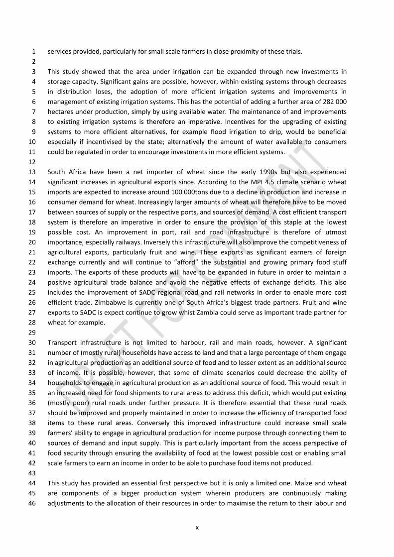
This study showed that the area under irrigation can be expanded through new investments in 3
storage capacity. Significant gains are possible, however, within existing systems through decreases 4
in distribution loses, the adoption of more efficient irrigation systems and improvements in 5
management of existing irrigation systems. This has the potential of adding a further area of 282 000 6
hectares under production, simply by using available water. The maintenance of and improvements 7
to existing irrigation systems is therefore an imperative. Incentives for the upgrading of existing 8
systems to more efficient alternatives, for example flood irrigation to drip, would be beneficial 9
especially if incentivised by the state; alternatively the amount of water available to consumers 10
could be regulated in order to encourage investments in more efficient systems. 11
12
South Africa have been a net importer of wheat since the early 1990s but also experienced 13
significant increases in agricultural exports since. According to the MPI 4.5 climate scenario wheat 14
imports are expected to increase around 100 000tons due to a decline in production and increase in 15
consumer demand for wheat. Increasingly larger amounts of wheat will therefore have to be moved 16
between sources of supply or the respective ports, and sources of demand. A cost efficient transport 17
system is therefore an imperative in order to ensure the provision of this staple at the lowest 18
possible cost. An improvement in port, rail and road infrastructure is therefore of utmost 19
importance, especially railways. Inversely this infrastructure will also improve the competitiveness of 20
agricultural exports, particularly fruit and wine. These exports as significant earners of foreign 21
exchange currently and will continue to “afford” the substantial and growing primary food stuff 22
imports. The exports of these products will have to be expanded in future in order to maintain a 23
positive agricultural trade balance and avoid the negative effects of exchange deficits. This also 24
includes the improvement of SADC regional road and rail networks in order to enable more cost 25
efficient trade. Zimbabwe is currently one of South Africa’s biggest trade partners. Fruit and wine 26
exports to SADC is expect continue to grow whist Zambia could serve as important trade partner for 27
wheat for example. 28
29
Transport infrastructure is not limited to harbour, rail and main roads, however. A significant 30
number of (mostly rural) households have access to land and that a large percentage of them engage 31
in agricultural production as an additional source of food and to lesser extent as an additional source 32
of income. It is possible, however, that some of climate scenarios could decrease the ability of 33
households to engage in agricultural production as an additional source of food. This would result in 34
an increased need for food shipments to rural areas to address this deficit, which would put existing 35
(mostly poor) rural roads under further pressure. It is therefore essential that these rural roads 36
should be improved and properly maintained in order to increase the efficiency of transported food 37
items to these rural areas. Conversely this improved infrastructure could increase small scale 38
farmers’ ability to engage in agricultural production for income purpose through connecting them to 39
sources of demand and input supply. This is particularly important from the access perspective of 40
food security through ensuring the availability of food at the lowest possible cost or enabling small 41
scale farmers to earn an income in order to be able to purchase food items not produced. 42
43
This study has provided an essential first perspective but it is only a limited one. Maize and wheat 44
are components of a bigger production system wherein producers are continuously making 45
adjustments to the allocation of their resources in order to maximise the return to their labour and 46

xi
capital. A study that follows an integrated approach to a much larger number of commodities is 1
therefore needed. The expected trend in expanded soybean and canola production serves as a good 2
example of shits not reflected in this study. 3
4
One of the major trends identified is that of a continuation of the increase in wheat imports, a trend 5
that will be accelerated within some of the climate scenarios. The sector has been able maintain a 6
positive agricultural trade balance despite the increase in wheat and other imports, mainly due to 7
the strong growth in fruit and wine exports. A failure to maintain a positive trade balance will result 8
in depreciation of the Rand that in turn will result in increases in the prices of the large and growing 9
amounts of imported wheat (and rice of which 100% is imported). Ultimately this could reduce 10
access to food due to reduced affordability. 11
12
The fruit and wine sectors are perceived to be under greater risk from climate change due to their 13
sensitivity to temperature increases. Future research on the climate impacts on these crops is 14
therefore very important, and should be linked to an understanding of the economic impacts, 15
including vulnerability to possible punitive tariffs due to the carbon intensity of international 16
transport. Various strategies directed towards the expansion of the competitiveness of these 17
industries are an essential adaptation strategy and a topic also in need of future research. 18
19
The narrow focus of current research on maize and wheat production may be a result of the 20
conflation between food security and food self-sufficiency. Given the current imports of wheat, the 21
inability to increase production and the expected increase in demand puts self-sufficiency clearly of 22
the table. An integrated approach to the availability and affordability aspects of food is therefore 23
much needed in future research. 24
25
1
1 Introduction 1
There have been many studies on the effects of potential climate change on agricultural yields 2
particularly of maize in South and Southern Africa. However, what these studies lack is an integrated 3
view of how the agricultural and food system would be affected under climate change due to the 4
many complex social and economic feedbacks involved. Therefore a key need is to translate the 5
respective climate scenarios into economic impacts, both in terms of the food access (price) 6
perspective of food security but also in terms of the impact on the decision to produce, which 7
impacts on agricultural employment. This study aims to fill this gap through a partial equilibrium 8
modelling approach in order to provide high level messages on the impact of climate change on 9
South African maize and wheat production. 10
11
The International Food Policy Research Institute (IFPRI) has conducted some of the most 12
comprehensive regional and global studies on the possible impacts of climate change on agricultural 13
production and food security. A study by Nelson et al. (2009) developed possible food security 14
scenarios towards 2050 through the use their International Model for Policy Analysis of Agricultural 15
Commodities and Trade (IMPACT), which incorporates the Decision Support System for 16
Agrotechnology Transfer (DSSAT) biophysical crop simulation model. Within these models they 17
incorporated the results of two climate models in order to generate projections. These where the 18
National Centre for Atmospheric Research (NCAR) model from the USA and the Commonwealth 19
Scientific and Industrial Research Organization (CSIRO) model from Australia. Both assume the A2 20
scenario of the IPCC’s Fourth Assessment and predict a warmer climate (higher temperatures) 21
towards 2050 with an increase in both evaporation and total precipitation. The extent the expected 22
increases in precipitation show a wide disparity, however, with the NCAR model forecasting an 23
average increase of about 10%, compared to CSIRO’s 2%. 24
25
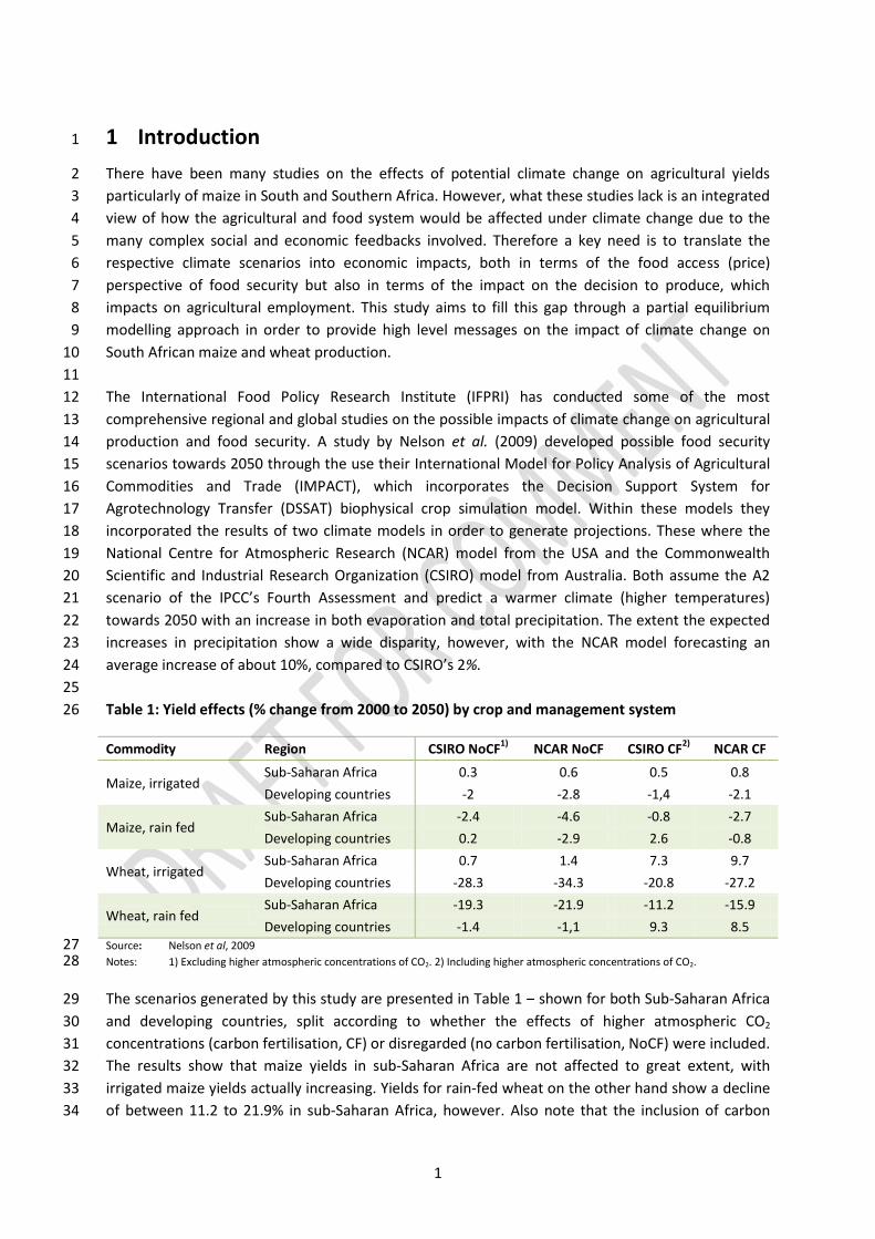
Table 1: Yield effects (% change from 2000 to 2050) by crop and management system 26
Commodity Region CSIRO NoCF1)
NCAR NoCF CSIRO CF2)
NCAR CF
Maize, irrigated Sub-Saharan Africa 0.3 0.6 0.5 0.8
Developing countries -2 -2.8 -1,4 -2.1
Maize, rain fed Sub-Saharan Africa -2.4 -4.6 -0.8 -2.7
Developing countries 0.2 -2.9 2.6 -0.8
Wheat, irrigated Sub-Saharan Africa 0.7 1.4 7.3 9.7
Developing countries -28.3 -34.3 -20.8 -27.2
Wheat, rain fed Sub-Saharan Africa -19.3 -21.9 -11.2 -15.9
Developing countries -1.4 -1,1 9.3 8.5 Source: Nelson et al, 2009 27 Notes: 1) Excluding higher atmospheric concentrations of CO2. 2) Including higher atmospheric concentrations of CO2. 28
The scenarios generated by this study are presented in Table 1 ‒ shown for both Sub-Saharan Africa 29
and developing countries, split according to whether the effects of higher atmospheric CO2 30
concentrations (carbon fertilisation, CF) or disregarded (no carbon fertilisation, NoCF) were included. 31
The results show that maize yields in sub-Saharan Africa are not affected to great extent, with 32
irrigated maize yields actually increasing. Yields for rain-fed wheat on the other hand show a decline 33
of between 11.2 to 21.9% in sub-Saharan Africa, however. Also note that the inclusion of carbon 34
2
fertilisation results in an increase or lower decrease in production than what is the case with the 1
without scenario. Ringler et al. (2010) concurs that wheat production will be most affected, their 2
results show an expected decline of just over 20%. 3
4
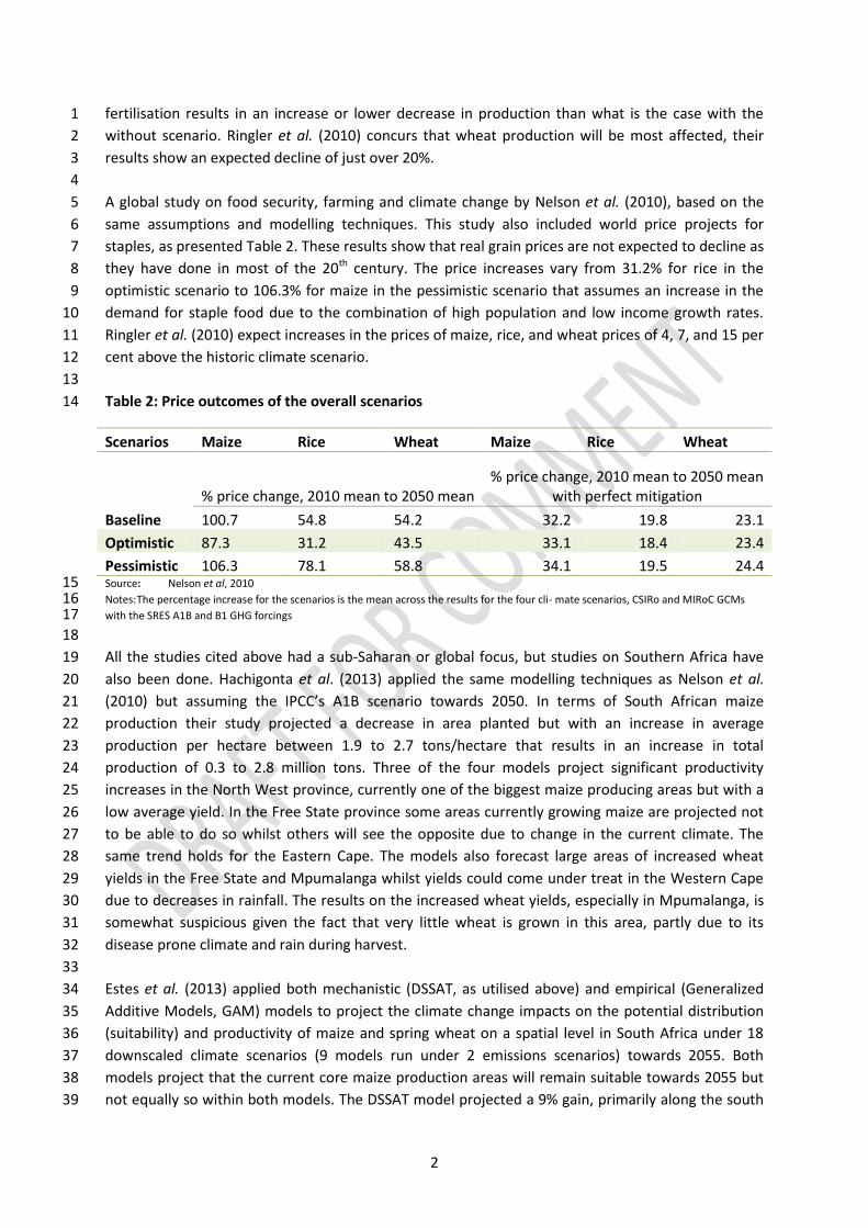
A global study on food security, farming and climate change by Nelson et al. (2010), based on the 5
same assumptions and modelling techniques. This study also included world price projects for 6
staples, as presented Table 2. These results show that real grain prices are not expected to decline as 7
they have done in most of the 20th century. The price increases vary from 31.2% for rice in the 8
optimistic scenario to 106.3% for maize in the pessimistic scenario that assumes an increase in the 9
demand for staple food due to the combination of high population and low income growth rates. 10
Ringler et al. (2010) expect increases in the prices of maize, rice, and wheat prices of 4, 7, and 15 per 11
cent above the historic climate scenario. 12
13
Table 2: Price outcomes of the overall scenarios 14
Scenarios Maize Rice Wheat Maize Rice Wheat
% price change, 2010 mean to 2050 mean
% price change, 2010 mean to 2050 mean with perfect mitigation
Baseline 100.7 54.8 54.2 32.2 19.8 23.1
Optimistic 87.3 31.2 43.5 33.1 18.4 23.4
Pessimistic 106.3 78.1 58.8 34.1 19.5 24.4 Source: Nelson et al, 2010 15 Notes: The percentage increase for the scenarios is the mean across the results for the four cli- mate scenarios, CSIRo and MIRoC GCMs 16 with the SRES A1B and B1 GHG forcings 17
18
All the studies cited above had a sub-Saharan or global focus, but studies on Southern Africa have 19
also been done. Hachigonta et al. (2013) applied the same modelling techniques as Nelson et al. 20
(2010) but assuming the IPCC’s A1B scenario towards 2050. In terms of South African maize 21
production their study projected a decrease in area planted but with an increase in average 22
production per hectare between 1.9 to 2.7 tons/hectare that results in an increase in total 23
production of 0.3 to 2.8 million tons. Three of the four models project significant productivity 24
increases in the North West province, currently one of the biggest maize producing areas but with a 25
low average yield. In the Free State province some areas currently growing maize are projected not 26
to be able to do so whilst others will see the opposite due to change in the current climate. The 27
same trend holds for the Eastern Cape. The models also forecast large areas of increased wheat 28
yields in the Free State and Mpumalanga whilst yields could come under treat in the Western Cape 29
due to decreases in rainfall. The results on the increased wheat yields, especially in Mpumalanga, is 30
somewhat suspicious given the fact that very little wheat is grown in this area, partly due to its 31
disease prone climate and rain during harvest. 32
33
Estes et al. (2013) applied both mechanistic (DSSAT, as utilised above) and empirical (Generalized 34
Additive Models, GAM) models to project the climate change impacts on the potential distribution 35
(suitability) and productivity of maize and spring wheat on a spatial level in South Africa under 18 36
downscaled climate scenarios (9 models run under 2 emissions scenarios) towards 2055. Both 37
models project that the current core maize production areas will remain suitable towards 2055 but 38
not equally so within both models. The DSSAT model projected a 9% gain, primarily along the south 39
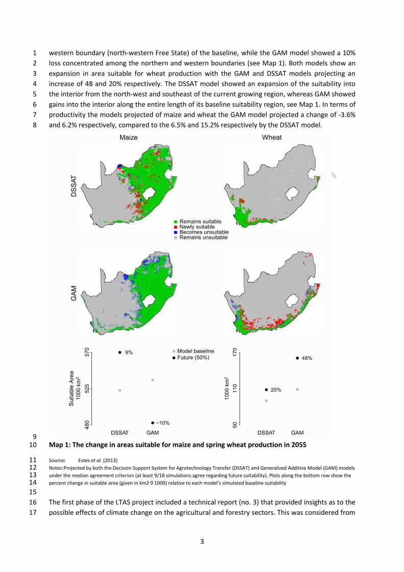
3
western boundary (north-western Free State) of the baseline, while the GAM model showed a 10% 1
loss concentrated among the northern and western boundaries (see Map 1). Both models show an 2
expansion in area suitable for wheat production with the GAM and DSSAT models projecting an 3
increase of 48 and 20% respectively. The DSSAT model showed an expansion of the suitability into 4
the interior from the north-west and southeast of the current growing region, whereas GAM showed 5
gains into the interior along the entire length of its baseline suitability region, see Map 1. In terms of 6
productivity the models projected of maize and wheat the GAM model projected a change of -3.6% 7
and 6.2% respectively, compared to the 6.5% and 15.2% respectively by the DSSAT model. 8
9 Map 1: The change in areas suitable for maize and spring wheat production in 2055 10
Source: Estes et al. (2013) 11 Notes: Projected by both the Decision Support System for Agrotechnology Transfer (DSSAT) and Generalized Additive Model (GAM) models 12 under the median agreement criterion (at least 9/18 simulations agree regarding future suitability). Plots along the bottom row show the 13 percent change in suitable area (given in km2 9 1000) relative to each model’s simulated baseline suitability 14
15
The first phase of the LTAS project included a technical report (no. 3) that provided insights as to the 16
possible effects of climate change on the agricultural and forestry sectors. This was considered from 17

4
biophysical perspective, specifically relating to yields and changes in the climatically optimum 1
growth areas. These models illustrated a wide range of possible impacts on dry land maize yield ‒ 2
ranging from a decrease in 25% to an increase of 10% depending on the scenario.1 Assuming a CO2 3
stabilisation at 450 ppm delivers results on yield impact of between -10% to +5%. The study finds 4
similar results on wheat and sunflower. The study also evaluated the impact on other agricultural 5
crops and grazing, as well as forestry production but all fall beyond the scope of this study. The study 6
also provided possible adaptation responses, which will be returned to in the last section of this 7
report, and highlighted future research needs (LTAS, 2013). 8
9
Given the above it clear that little consensus exists between the various studies but some broad 10
trends can be identified, however. 11
2 Methodology 12
The BFAP sector model is used to evaluate the effect of climate scenario’s on the price, trade and 13
production effects on these key staple crops. These results will in turn be incorporated into the BFAP 14
consumer models in order to evaluate the effect of the possible price changes especially on poorer 15
households in South Africa. The data will also be incorporated into the BFAP employment model in 16
order explore the employment effects of the scenario’s on employment within the maize and wheat 17
industries. 18
2.1 The sector model 19
Section 3 presents the results obtained through the BFAP sector model. This model was first utilised 20
in 2003 and can be described as an econometric, recursive partial equilibrium model of the South 21
African agricultural sector, which presently covers 52 commodities. Within each sector, the 22
components of supply and demand are estimated and equilibrium is established based on balance 23
sheet principles, where demand equals supply at national level. The model is solved within a closed 24
system of equations, where grains are linked to livestock through feed, implying that a shock in the 25
livestock sector is transmitted to grains and oilseeds and vice versa. The model is linked to global 26
markets through the Food and Agricultural Policy Research Institute (FAPRI) in America, as well as 27
the Aglink-Cosimo modelling system used for the annual OECD-FAO agricultural outlook. 28
Figure 1 presents a diagram of the BFAP modelling system where weather is captured as an external 29
driver of the BFAP sector model. 30
31
1 Depending on the scenario, with unconstrained emissions (typified by IPCC SRES A2 and IPCC AR5 8.5 W.m-2
RCP) and constrained emissions (typified by IPCC SRES B1 and IPCC AR5 4. 5 W. m-2 RCP).

5
1 Figure 1: The BFAP modelling system 2
The BFAP sector model does take biophysical elements, specifically rainfall, into account but does 3
not provide for temperature and CO2 fertilisation effects. Within this study it is assumed that the 4
negative effects of increased temperature are offset by the positive effects of CO2 fertilisation. Given 5
the results of the study by Nelson et al. (2010) discussed in Section 1 it can be assumed that carbon 6
fertilisation has a net positive effect on both wheat and maize yield. Within the model rainfall serves 7
as one of the variables that impacts on the decision to plant and eventually also impacts on the yield 8
realised by the respective crops. For this purpose precipitation in certain production areas for 9
certain months of the year is taken into account in the model. 10
11
For the purpose of this study the BFAP sector model can only be extended meaningfully to 2030 due 12
to the fact that model consists of a number of forecasted macro independent variables that are 13
currently only forecasted up to 2023 (typical 10-year outlook) and in some isolated cases up to 2030 14
by the international modelling institutions. From the long-run projections it also becomes evident 15
that beyond a certain period, a long-run equilibrium is established among markets and trends are 16
mostly unchanged until a new exogenous shock is introduced into the model. 17
2.2 Consumer Impact study 18
Section 4 presents the results of the consumer impact study. Within this study the retail prices for 19
maize meal and bread generated through the BFAP retail price transmission models will serve as the 20
main input for this analysis. The potential impact of maize and wheat price changes due to climate 21
change, especially on poorer households in South Africa will be investigated with multiple 22
approaches. 23
24
6
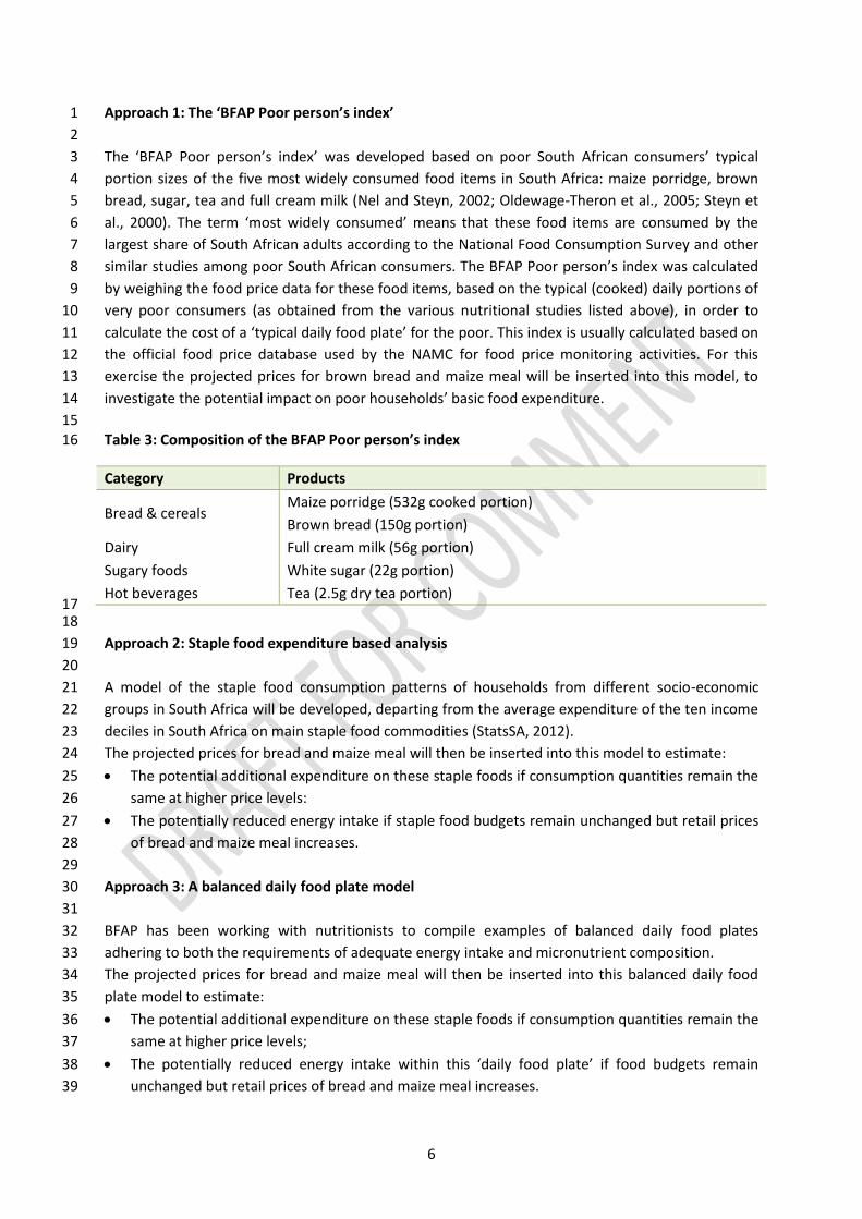
Approach 1: The ‘BFAP Poor person’s index’ 1
2
The ‘BFAP Poor person’s index’ was developed based on poor South African consumers’ typical 3
portion sizes of the five most widely consumed food items in South Africa: maize porridge, brown 4
bread, sugar, tea and full cream milk (Nel and Steyn, 2002; Oldewage-Theron et al., 2005; Steyn et 5
al., 2000). The term ‘most widely consumed’ means that these food items are consumed by the 6
largest share of South African adults according to the National Food Consumption Survey and other 7
similar studies among poor South African consumers. The BFAP Poor person’s index was calculated 8
by weighing the food price data for these food items, based on the typical (cooked) daily portions of 9
very poor consumers (as obtained from the various nutritional studies listed above), in order to 10
calculate the cost of a ‘typical daily food plate’ for the poor. This index is usually calculated based on 11
the official food price database used by the NAMC for food price monitoring activities. For this 12
exercise the projected prices for brown bread and maize meal will be inserted into this model, to 13
investigate the potential impact on poor households’ basic food expenditure. 14
15 Table 3: Composition of the BFAP Poor person’s index 16
Category Products
Bread & cereals Maize porridge (532g cooked portion)
Brown bread (150g portion)
Dairy Full cream milk (56g portion)
Sugary foods White sugar (22g portion)
Hot beverages Tea (2.5g dry tea portion) 17 18
Approach 2: Staple food expenditure based analysis 19
20
A model of the staple food consumption patterns of households from different socio-economic 21
groups in South Africa will be developed, departing from the average expenditure of the ten income 22
deciles in South Africa on main staple food commodities (StatsSA, 2012). 23
The projected prices for bread and maize meal will then be inserted into this model to estimate: 24
The potential additional expenditure on these staple foods if consumption quantities remain the 25
same at higher price levels: 26
The potentially reduced energy intake if staple food budgets remain unchanged but retail prices 27
of bread and maize meal increases. 28
29
Approach 3: A balanced daily food plate model 30
31
BFAP has been working with nutritionists to compile examples of balanced daily food plates 32
adhering to both the requirements of adequate energy intake and micronutrient composition. 33
The projected prices for bread and maize meal will then be inserted into this balanced daily food 34
plate model to estimate: 35
The potential additional expenditure on these staple foods if consumption quantities remain the 36
same at higher price levels; 37
The potentially reduced energy intake within this ‘daily food plate’ if food budgets remain 38
unchanged but retail prices of bread and maize meal increases. 39

7
Developing future scenarios with respect to a change in household characteristics such as food 1
expenditure patterns, class mobility and others, falls beyond the scope of this study. Hence, the 2
current characteristics will be applied in order to generate the impact of future maize meal and 3
bread prices in the analyses described above. Thus, the assumption will have to be made that 4
households will have the same characteristics 20 years into the future as is presently the case. 5
2.3 Climate Data 6
The LTAS Phase 1 developed a consensus view on the range of plausible climate scenarios for three 7
time-periods for South Africa at national and sub-national scales under a range of global emissions 8
scenarios. The time-periods considered were 2015 to 2035 (centred on ~2025, so-called short- term) 9
in addition to the previously followed approach of exploring climate change over several decades 10
into the future (centred on ~2050 (medium-term) and ~2090 (long-term). 11
12
These scenarios were developed through local and international climate modelling expertise using 13
both statistical and dynamical downscaling methodologies based on outputs from IPCC AR4 (A2 and 14
B1 emissions scenarios) and IPCC AR5 (RCP 8.5 and 4.5 Wm-2 pathways). These represent an 15
unmitigated future energy pathway (unconstrained, A2 and RCP8.5) and mitigated future energy 16
pathway (constrained, B1 and RCP4.5, or emissions scenarios equivalent to CO2 levels stabilising 17
between 450 and 500ppm). 18
19
South Africa’s climate future up to 2050 and beyond can be described by using four fundamental 20
climate scenarios at national scale, with different degrees of change and likelihood that capture the 21
impacts of global mitigation and the passing of time. 22
23
1. warmer (<3°C above 1961–2000) and wetter with greater frequency of extreme rainfall 24
events. 25
2. warmer (<3°C above 1961–2000) and drier, with an increase in the frequency of drought 26
events and somewhat greater frequency of extreme rainfall events. 27
3. hotter (>3°C above 1961–2000) and wetter with substantially greater frequency of extreme 28
rainfall events. 29
4. hotter (>3°C above 1961–2000) and drier, with a substantial increase in the frequency of 30
drought events and greater frequency of extreme rainfall events. 31
32
The effect of strong international mitigation responses would be to reduce the likelihood of 33
scenarios 3 and 4. It is not possible to evaluate the effect of all the respective climate models 34
through the use of the BFAP model during the time frame of LTAs phase 2 due to the amount of 35
work required to prepare the data for analysis. It was therefore decided to conduct a preliminary 36
test of the effect of four climate models representing a range of rainfall changes at the national 37
level. A subset of scenarios was selected from those available to explore the vulnerability of wheat 38
and maize production and its effect on the food system. 39
40

8
1 Table 4: LTAS Scenario Representative Models (2040-2050) with calculated percentage average 2
rainfall changes 3
LTAS Scenario Model Avg. change in
MAP (%)
Warmer/moderately drier ACCESS RCP 4.5 - 3.3%
Warmer/drier MPI RCP 4.5 - 1.1%
Hotter/moderately drier ACCESS RCP 8.5 - 4.3%
Hotter/drier MPI RCP 8.5 - 14%
Source: Aurecon (2014) 4
5
In light of the above, four CSIR CMIP5 climate models (see Table 4) were selected and the results 6
incorporated into the BFAP sector model in order to evaluate the possible price and production 7
impacts of each of these possible climate futures. The warmer models incorporate the assumptions 8
of the RCP 4.5 climate futures whilst the hotter scenarios assume the RCP 8.5 futures. Both of the 9
moderately drier scenarios are the result of the ACCESS global climate model whilst the drier 10
scenarios are the result of the MPI global model. 11
12
These models delivered actual monthly precipitation, dynamically downscaled through the CCAM 13
(conformal-cubic atmospheric model) into quaternary catchments. These quaternary catchments in 14
turn where aggregated into secondary catchments by averaging the quaternaries that constitute 15
each of the secondary catchments. The resulting secondary catchments where then grouped in 16
according to production areas and months of interest specified by the BFAP sector model. With the 17
wheat model for example, both the winter (Western Cape) and summer (Free State) production 18
areas where compared with the calculated secondary catchments, the relevant catchments within 19
each of these production areas where then identified, the precipitation data on the relevant months 20
isolated, totalled per production area and then included in the model. 21
22
As stated above this model can only provide meaningful econometric results up to 2030 due the fact 23
that forecasted data on the determining factors (dependent variables) of the model, other than 24
precipitation in this case, is only available up to this date. The problem, however, is that an analysis 25
of the precipitation data of the respective models, grouped in accordance the BFAP model, show a 26
high correlation before 2030 and only show a significant divergence thereafter. In other words, it is 27
apparent that for some of the scenarios the effects on precipitation increase towards the end period 28
(2050). Therefore, in order to analyse the potential economic impacts of climate on the South 29
African maize and wheat industries, the precipitation data projected for the period 2034 to 2050 is 30
introduced in the BFAP sector model for each of the scenarios, which is then compared to a base 31
case. The BFAP sector model generates absolute and percentage shocks to illustrate the relative 32
deviations from the base. The implication thereof can be best described as the effect of more than 33
20 years of climate change on the current context. 34
35
It was decided to use actual historic precipitation data as a base to which the modelling results of 36
the respective scenarios could be compared. For this purpose the rainfall for the period 1950 to 37
2000 was used, this data was also aggregated to secondary catchments, and allocated to the 38
relevant production areas as explained above and included in the model. The modelling results of 39
this data hence serves as a “real world” stochastic base to which the other results can be compared. 40
9
3 Climate Change Impacts on Production and Prices 1
3.1 Developing the LTAS BASE 2030 projections 2
Various approaches and modelling techniques can be applied in the world of foresighting and 3
developing future outcomes of agricultural markets. The methodology that BFAP has developed links 4
scenario thinking techniques to a set of empirical models at global, national and farm level. The 5
starting point for the empirical impact analyses is first to set a benchmark from where potential 6
deviations can be measured. For BFAP, this benchmark is the most basic projections that are 7
simulated in the BFAP sector model and are referred to as deterministic baseline projections. As 8
discussed in section 2.1 of this report, the BFAP sector model is a recursive partial equilibrium 9
model. The model takes the interaction between various industries like livestock, grains and oilseeds 10
into consideration and projects the future equilibrium between demand and supply for a range of 11
agricultural markets subject to a set of assumptions. 12
13
Traditionally the BFAP baseline projections provide a 10-year outlook of commodity markets, yet for 14
the purpose of this study, this baseline is extended to 2030. In other words, a future scenario is 15
simulated for the next 17 years that is grounded in a series of assumptions about the general 16
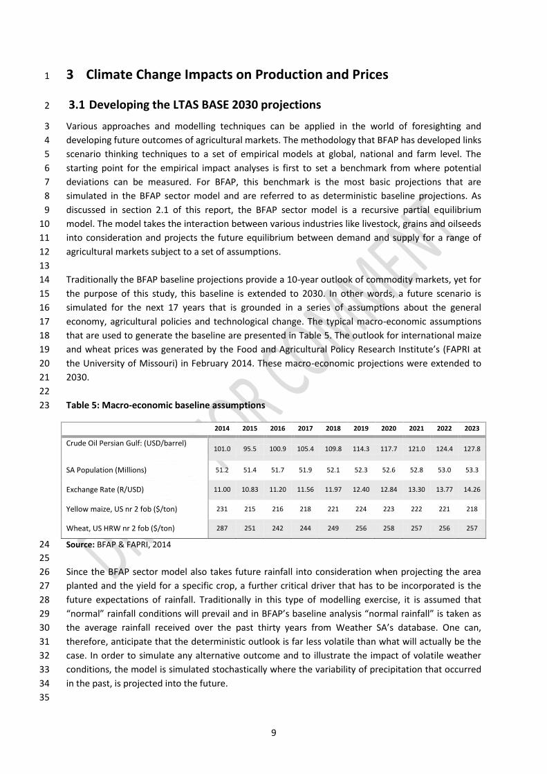
economy, agricultural policies and technological change. The typical macro-economic assumptions 17
that are used to generate the baseline are presented in Table 5. The outlook for international maize 18
and wheat prices was generated by the Food and Agricultural Policy Research Institute’s (FAPRI at 19
the University of Missouri) in February 2014. These macro-economic projections were extended to 20
2030. 21
22
Table 5: Macro-economic baseline assumptions 23
2014 2015 2016 2017 2018 2019 2020 2021 2022 2023
Crude Oil Persian Gulf: (USD/barrel)
101.0 95.5 100.9 105.4 109.8 114.3 117.7 121.0 124.4 127.8
SA Population (Millions) 51.2 51.4 51.7 51.9 52.1 52.3 52.6 52.8 53.0 53.3
Exchange Rate (R/USD) 11.00 10.83 11.20 11.56 11.97 12.40 12.84 13.30 13.77 14.26
Yellow maize, US nr 2 fob ($/ton) 231 215 216 218 221 224 223 222 221 218
Wheat, US HRW nr 2 fob ($/ton) 287 251 242 244 249 256 258 257 256 257
Source: BFAP & FAPRI, 2014 24
25
Since the BFAP sector model also takes future rainfall into consideration when projecting the area 26
planted and the yield for a specific crop, a further critical driver that has to be incorporated is the 27
future expectations of rainfall. Traditionally in this type of modelling exercise, it is assumed that 28
“normal” rainfall conditions will prevail and in BFAP’s baseline analysis “normal rainfall” is taken as 29
the average rainfall received over the past thirty years from Weather SA’s database. One can, 30
therefore, anticipate that the deterministic outlook is far less volatile than what will actually be the 31
case. In order to simulate any alternative outcome and to illustrate the impact of volatile weather 32
conditions, the model is simulated stochastically where the variability of precipitation that occurred 33
in the past, is projected into the future. 34
35
10
For the purpose of this study, a different approach is followed, where the LTAS base precipitation is 1
used in the model to develop a benchmark to which the modelling results of the respective scenarios 2
can be compared. It was decided to use actual historic precipitation data as the base. For this 3
purpose the rainfall for the period 1950 to 2000 was used and aggregated to secondary catchments, 4
and allocated to the relevant production areas as explained in section 2 of this report. The modelling 5
results of this data hence serve as a “real world” stochastic base to which the other results can be 6
compared. 7
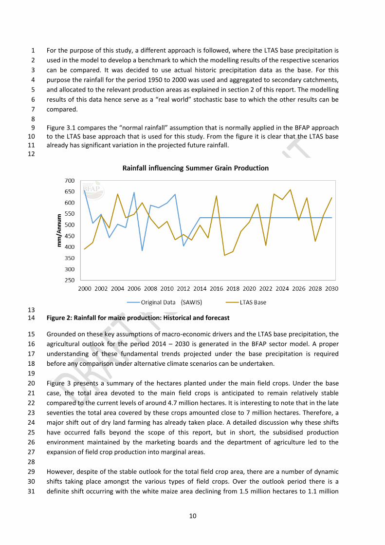
8 Figure 3.1 compares the “normal rainfall” assumption that is normally applied in the BFAP approach 9 to the LTAS base approach that is used for this study. From the figure it is clear that the LTAS base 10 already has significant variation in the projected future rainfall. 11 12
13 Figure 2: Rainfall for maize production: Historical and forecast 14
Grounded on these key assumptions of macro-economic drivers and the LTAS base precipitation, the 15
agricultural outlook for the period 2014 – 2030 is generated in the BFAP sector model. A proper 16
understanding of these fundamental trends projected under the base precipitation is required 17
before any comparison under alternative climate scenarios can be undertaken. 18
19
Figure 3 presents a summary of the hectares planted under the main field crops. Under the base 20
case, the total area devoted to the main field crops is anticipated to remain relatively stable 21
compared to the current levels of around 4.7 million hectares. It is interesting to note that in the late 22
seventies the total area covered by these crops amounted close to 7 million hectares. Therefore, a 23
major shift out of dry land farming has already taken place. A detailed discussion why these shifts 24
have occurred falls beyond the scope of this report, but in short, the subsidised production 25
environment maintained by the marketing boards and the department of agriculture led to the 26
expansion of field crop production into marginal areas. 27
28
However, despite of the stable outlook for the total field crop area, there are a number of dynamic 29
shifts taking place amongst the various types of field crops. Over the outlook period there is a 30
definite shift occurring with the white maize area declining from 1.5 million hectares to 1.1 million 31

11
hectares and the soybean area doubling from around 500 000ha to more than 1 million hectares. 1
Farmers will plant more yellow maize and the area under sunflower is expected to remain relatively 2
constant. Therefore, the oilseed area is anticipated to expand at the costs of grains. 3
4 Figure 3: SA main field crop area 5
The amount of dry land wheat planted in the Free State and parts of Limpopo and the North West 6
has declined drastically from levels close to 1 million hectares in the late nineties shortly after the 7
abolishment of the marketing boards to less than 200 000ha in 2013. Basic economic principles have 8
been the key driver behind this dramatic shift with the profitability of maize and lately soybeans 9
outstripping that of wheat, mainly due to the introduction of new genetically modified seed varieties 10
boosting the yields of maize and soybeans at a much faster rate. A further driver behind the shift in 11
area can also be attributed to the increased levels of risk aversion of farmers in the deregulated 12
marketing environment where wheat yields in these areas are more exposed to climatic risks such as 13
late frost or rain that is not received in time. In recent years, excessive precipitation in November 14
and December during harvest increased crop losses and decreased the quality of wheat delivered. In 15
other words, farmers are already adapting in order to mitigate their risk due to climate variability 16
and volatile markets. 17
18
Although the area under dry land wheat production in the Western Cape has also gradually declined 19
over the past decade, the shift has not been nearly as dramatic, with the area stabilizing around 20
300 000ha. However, over the baseline it is anticipated the some hectares in this production region 21
will be lost to rotation production practises with canola. Significant strides have been made in recent 22
years to improve the yields of canola and the introduction of genetically modified canola will bring 23
significant relief to significant weed pressure experienced by wheat farmers. 24
25
The long term cropping patterns that are portrayed in Figure 3 are simulated based on the dynamic 26
interaction between demand and supply, which basically determines the equilibrium pricing 27
conditions. Equilibrium pricing conditions drive the impact of exogenous shocks on commodity 28
markets. The focus in this research falls on maize and wheat, where the equilibrium pricing 29
12
conditions differ significantly. Even within the maize market, there is a difference in the way that 1
yellow and white maize prices, for example, relate to international prices. In short, under free 2
market conditions, domestic prices tend to trade closer to export parity when local supply exceeds 3
local demand by a significant margin and there is a tradable surplus. If, however, there is a shortfall 4
in the local market and local demand can only be met by imports, the domestic price tends to trade 5
at import parity. Therefore, in a free market, local prices are expected to trade between import and 6
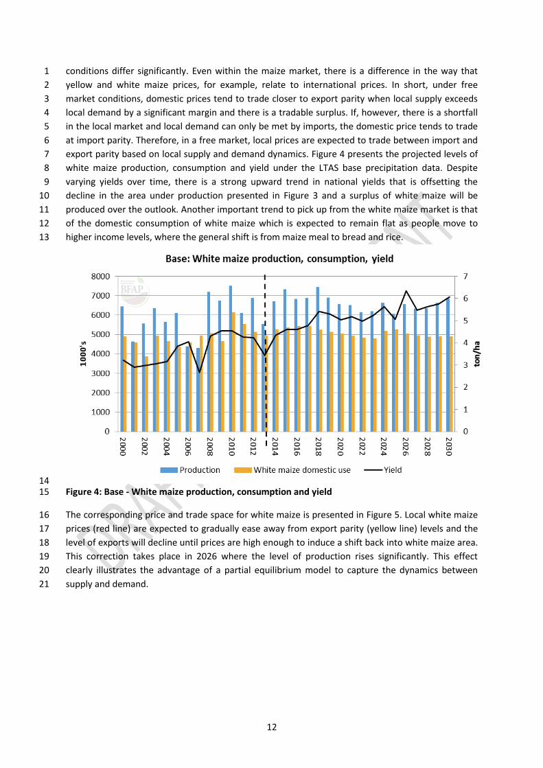
export parity based on local supply and demand dynamics. Figure 4 presents the projected levels of 7
white maize production, consumption and yield under the LTAS base precipitation data. Despite 8
varying yields over time, there is a strong upward trend in national yields that is offsetting the 9
decline in the area under production presented in Figure 3 and a surplus of white maize will be 10
produced over the outlook. Another important trend to pick up from the white maize market is that 11
of the domestic consumption of white maize which is expected to remain flat as people move to 12
higher income levels, where the general shift is from maize meal to bread and rice. 13
14 Figure 4: Base - White maize production, consumption and yield 15
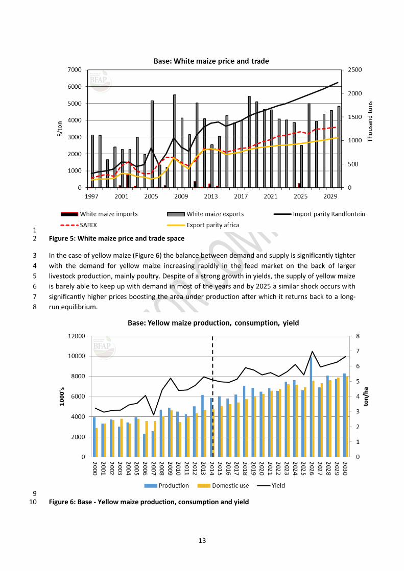
The corresponding price and trade space for white maize is presented in Figure 5. Local white maize 16
prices (red line) are expected to gradually ease away from export parity (yellow line) levels and the 17
level of exports will decline until prices are high enough to induce a shift back into white maize area. 18
This correction takes place in 2026 where the level of production rises significantly. This effect 19
clearly illustrates the advantage of a partial equilibrium model to capture the dynamics between 20
supply and demand. 21
13
1 Figure 5: White maize price and trade space 2
In the case of yellow maize (Figure 6) the balance between demand and supply is significantly tighter 3
with the demand for yellow maize increasing rapidly in the feed market on the back of larger 4
livestock production, mainly poultry. Despite of a strong growth in yields, the supply of yellow maize 5
is barely able to keep up with demand in most of the years and by 2025 a similar shock occurs with 6
significantly higher prices boosting the area under production after which it returns back to a long-7
run equilibrium. 8
9 Figure 6: Base - Yellow maize production, consumption and yield 10

14
Figure 7 presents the corresponding price and trade space for yellow maize. Due to the lower yields 1
projected over the period 2018 – 2021 (induced by lower precipitation in the LTAS base) the level of 2
yellow maize exports plummet and the local market corresponds with more volatility in the market 3
compared to white maize. Naturally, in the feed market yellow maize can be substituted with white 4
maize with a slight price premium and therefore the level of correlation between these two markets 5
will remain high. 6
7 Figure 7: Base Yellow maize price and trade space 8
Contrary to white and yellow maize, SA is a net importer of wheat and the level of wheat imports are 9
expected to rise with consumption reaching more than 4 million tons by 2030 and the level of 10
production fluctuating around 1.7 million tons. The majority of wheat that is locally consumed will 11
be imported. The general rise in per capita income and the rate of urbanization triggers strong 12
growth in the demand for bread, rice and potatoes. The historic trend in summer yields that is 13
presented in Figure 8 is misleading because the relative share of irrigation wheat increased rapidly as 14
the dryland hectares dwindled and that is the reason for the sharp rise in yields. Over the outlook 15
period, average yields will continue to increase and the dryland area is further consolidated and 16
irrigation will make up a larger share of the total area of wheat planted in the summer rainfall 17
region. 18
19
Wheat yields in the winter rainfall region (Western Cape) have been exceptional since 2010 with 20
above normal climatic conditions boosting average yields for the total region above 3t/ha in 2012. 21
Yields have already decline in 2013 with slightly less rain. Over the outlook period yields in the 22
winter rainfall area are expected to increase marginally. The reason for much lower yields in the 23
outlying years is simply due to lower projected precipitation levels under the LTAS base case. The 24
main drivers behind an increasing trend in yields are better rotational cropping patterns and the 25
exclusion of marginal soils. In total, the Western Cape is expected to lose almost 70 000 ha of wheat 26
over the baseline. 50 000 ha will be picked up by canola and the remaining hectares will go for 27
grazing purposes. 28

15
1 Figure 8: Base - Wheat production, consumption and yield 2
The price and trade space for the South African wheat market is presented in Figure 9. As can be 3
expected, the domestic wheat price is following the import parity price levels and will continue to do 4
so in future unless there is a major shift in trade policies that influences the equilibrium pricing 5
conditions. In fact, BFAP estimates show that the level of price transmission from international to 6
local market prices equals 92%. Hence, no local supply - or demand shock with have any major 7
impact on the price of wheat. The market will simply adjust the level of imports depending on the 8
expected shortfall. 9
10 Figure 9: Base - Wheat price and trade space 11
12
13

16
The wheat import parity price continues to increase along a linear trend. This is caused by the nature 1
of the projected global wheat price (Table 5) that was generated by FAPRI. The import parity price in 2
Rand terms increases as the Rand depreciates over time. 3
4 Case Study1: Maize
Figure 10 presents South Africa maize production in terms of area planted and average yield, expressed as a 5 year moving
average to better enable the observation of the trend. The figure clearly shows a decline in the area planted since 1988,
from its highest level of close to 5 million hectares in the mid-1980s to a low less than 2 million hectares in the mid-2000s,
a reduction of more than . Average yield increased from an average of around 1.5 tons/ha in the 1970s and 1980s to the
current level of around 4 tons/ha. Average yield shows a similar trend to that of area planted with it starting to increase at
a relatively slow rate since 1988 and then accelerating the mid-1990s.
The reduction in the area planted since 1988 is mainly the result of the deregulation of maize marketing through the
abolishment of the fixed price single channel marketing scheme. This resulted in the reduction of the domestic maize price
to export parity levels, which in turn lowered the profitability of marginal land in production to such an extent as to make it
unprofitable to produce on (Vink and Kirsten, 2000). Maize increases, especially during the late 1980s and early 1990s was
driven by this trend of the removal of marginal land from production, mainly in the more arid western production regions.
Sou
rce: DAS, (2013)
Figure 10: South African Maize: Area Planted and Yield (5 year moving averages)
Another major shift in summer production area, where almost all of the maize is grown, is that of the emergence of
soybeans as a significant crop. Production of this crop has grown from a negligible figure of 22 000 hectares in 1975 to 470
000 hectares in 2012. This exceed the 452 000 hectares under sunflower production during the same year. The production
of this crop has remained around this figure since the late 1980s.
Given the above one can conclude that more than 1 million hectares (2 million minus 0.5 million under soybean) of land
previously under maize production have been converted to planted pastures, natural grazing or lost to mining activity since
the late 1980s. A significant percentage of this land, even though marginal, could be reintroduced to maize production
given increased rainfall in the western production regions or an increase in the maize price due to domestic shortages.
5
6
7
8
9

17
3.2 Comparing the LTAS scenarios to the base 1
3.2.1 Maize 2
Given the comprehensive discussion of the fundamental maize and wheat trends under the base 3
case, alternative scenarios with altering precipitation levels can now be introduced in the BFAP 4
sector model and compared to the baseline. In the first place, it is however important to provide a 5
graphically representation of the scenarios that are highlighted in Table 4. Unlike the date presented 6
in the that table this data does not represent national MAPs but rather the relevant rainfall data 7
extracted from the national monthly quaternary data set in accordance to the respective maize 8
production regions. From Figure 11 it is evident that there is only one scenario where future 9
precipitation levels differ significantly from the base case, namely the MPI 4.5 scenario. It is 10
important to note that this scenario showed the lowest decline in national MAP. This highlights the 11
fact that both the timing and locality of rainfall are more important than national mean annual 12
precipitation rates. Hence, for the purpose of further discussions, only the modelling results of this 13
scenario will be presented. 14
15 Figure 11: Precipitation influencing maize production– base versus alternative scenarios 16
The various scenarios where introduced in the BFAP sector model in order to generate the potential 17
impact of the different precipitation levels on maize and wheat markets. Figure 12 shows how white 18
maize yields are anticipated to decline by 1.1t/ha on average over the outlook period resulting in a 19
drop in total production of approximately 1.6 million tons per annum and an increase in the white 20
maize prices of 16 percent (Figure 13). Similarly, yellow maize production will decline by 21
approximately 900 000tons per annum. Under this scenario South African maize exports will drop by 22
more than 1 million tons, which implies that the pressure of funding the foreign account deficit will 23
increasingly fall on other agricultural export produce like wine and fruits. 24
25
The interesting part of this scenario is that the area under maize production is expected to increase 26
by more than 200 000ha. This shift in hectares comes from the drop in yields that is more than offset 27
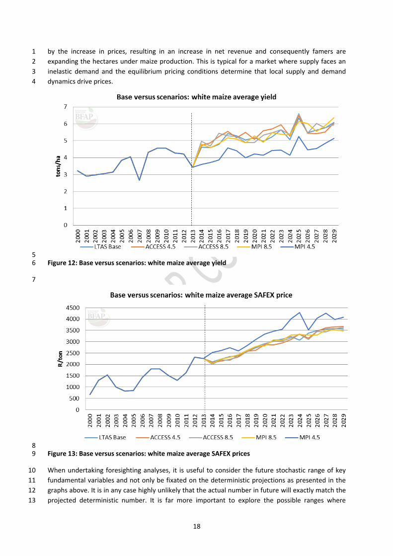
18
by the increase in prices, resulting in an increase in net revenue and consequently famers are 1
expanding the hectares under maize production. This is typical for a market where supply faces an 2
inelastic demand and the equilibrium pricing conditions determine that local supply and demand 3
dynamics drive prices. 4
5 Figure 12: Base versus scenarios: white maize average yield 6
7
8 Figure 13: Base versus scenarios: white maize average SAFEX prices 9
When undertaking foresighting analyses, it is useful to consider the future stochastic range of key 10
fundamental variables and not only be fixated on the deterministic projections as presented in the 11
graphs above. It is in any case highly unlikely that the actual number in future will exactly match the 12
projected deterministic number. It is far more important to explore the possible ranges where 13

19
variables can move. 1
2
For this exercise BFAP applies stochastic modelling techniques that can assist to generate a plausible 3
range of outcomes given the set of assumptions. Figure 14 and Figure 15 are comparing the base 4
case stochastic results to the stochastic results simulated under scenario MPI 4.5. Apart from 5
significantly lower precipitation levels under MPI 4.5, the range of rainfall that can be received is 6
significantly wider under the MPI 4.5 scenario compared to the base case. This increases the climatic 7
risks significantly. 8
9 Figure 14: Stochastic precipitation – Base versus MPI 4.5 10
Based on the distribution for future precipitation, the distribution of plausible maize prices is 11
significantly higher under MPI 4.5 than under the base case. Figure 13 illustrates that compared to 12
an average white maize price of around R3000/ton under the base case, the most likely white maize 13
price can increase to levels around R3700/ton under the MOI 4.5 scenario. 14
15 Figure 15: Stochastic white maize price – Base versus MPI 4.5 16
17
18
19

20
Case Study 2: Wheat
Figure 16 shows South African wheat production and domestic use patterns for the period 1994 to 2013. From this figure it
is clear that the domestic demand exceed the domestic supply, in 2013 for example, the 40% of the domestic demand
where imported. The price of wheat in South Africa will therefore be equal to the import parity (world price plus transport
cost to SA) price, unless the domestic production exceed the domestic demand. As indicated in section 1 Estes et al. (2013)
concluded that the area suitable for wheat production could expand between 20 and 48%, depending on the biophysical
model used. The models showed a possible productivity increase of between 6.5% and 15.2%. These changes have the
potential to increase domestic supply sufficiently to move South Africa towards a net exporter status. I this is not possible,
however, the discussion relating to wheat moves to one of the size of imports, the area under production and the yield,
because the local price will simply be equal to the world price plus transport.
Source: DAS, (2013); SAGIS, (2014)
Figure 16: South African Wheat Production and Domestic Use
1
3.2.2 Wheat 2
The impact of alternative future precipitation levels on the wheat market is significantly different 3
from the impact on the maize markets. The BFAP sector model makes a distinction between the 4
summer and winter rainfall areas. In the case of the winter rainfall area, the precipitation under 5
scenario MPI 4.5 is still lower compared to the base and the other scenarios that are simulated but 6
the difference is not as dramatic as was the case with maize, where the MPI 4.5 scenario presented 7
significantly lower precipitation levels. Figure 14 presents the future precipitation levels under the 8
LTAS base case and scenarios that will influence the production of wheat in the winter rainfall 9
region. 10

21
1 Figure 14: Precipitation influencing wheat production in winter rainfall region 2
For the precipitation levels influencing the production levels of wheat in the summer rainfall area, 3
the exact opposite is expected with much higher winter season precipitation levels projected under 4
the MPI 4.5 scenario compared to the base case and other scenarios (Figure 15). 5
6 Figure 15: Precipitation influencing wheat production in summer rainfall region 7
Therefore, although less rainfall is projected under MPI 4.5 for the summer area in the months 8
influencing maize production (December, January, February), the rainfall is expected to increase in 9
the winter months (July, August, September), which will have a positive impact on wheat yields. 10
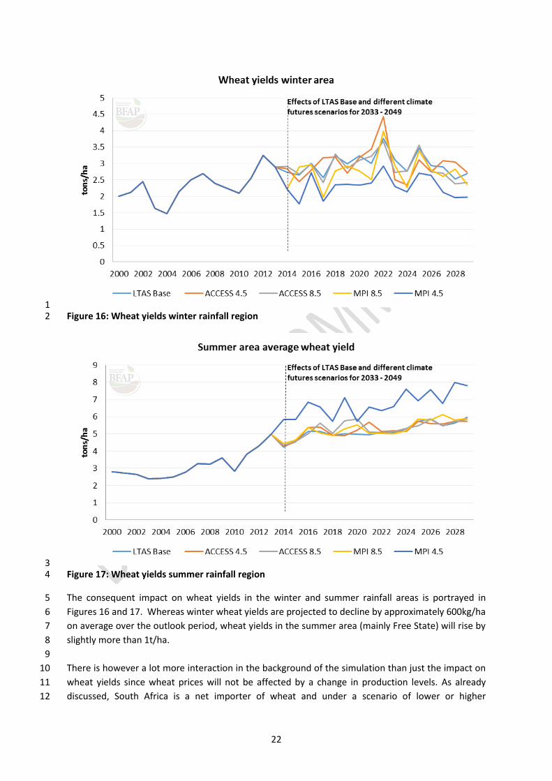
22
1 Figure 16: Wheat yields winter rainfall region 2
3 Figure 17: Wheat yields summer rainfall region 4
The consequent impact on wheat yields in the winter and summer rainfall areas is portrayed in 5
Figures 16 and 17. Whereas winter wheat yields are projected to decline by approximately 600kg/ha 6
on average over the outlook period, wheat yields in the summer area (mainly Free State) will rise by 7
slightly more than 1t/ha. 8
9
There is however a lot more interaction in the background of the simulation than just the impact on 10
wheat yields since wheat prices will not be affected by a change in production levels. As already 11
discussed, South Africa is a net importer of wheat and under a scenario of lower or higher 12
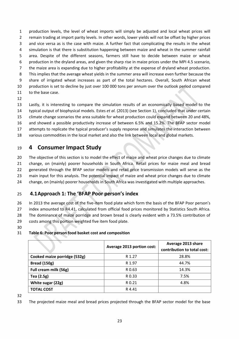
23
production levels, the level of wheat imports will simply be adjusted and local wheat prices will 1
remain trading at import parity levels. In other words, lower yields will not be offset by higher prices 2
and vice versa as is the case with maize. A further fact that complicating the results in the wheat 3
simulation is that there is substitution happening between maize and wheat in the summer rainfall 4
area. Despite of the different seasons, farmers still have to decide between maize or wheat 5
production in the dryland areas, and given the sharp rise in maize prices under the MPI 4.5 scenario, 6
the maize area is expanding due to higher profitability at the expense of dryland wheat production. 7
This implies that the average wheat yields in the summer area will increase even further because the 8
share of irrigated wheat increases as part of the total hectares. Overall, South African wheat 9
production is set to decline by just over 100 000 tons per annum over the outlook period compared 10
to the base case. 11
12
Lastly, it is interesting to compare the simulation results of an economically based model to the 13
typical output of biophysical models. Estes et al. (2013) (see Section 1), concluded that under certain 14
climate change scenarios the area suitable for wheat production could expand between 20 and 48%, 15
and showed a possible productivity increase of between 6.5% and 15.2%. The BFAP sector model 16
attempts to replicate the typical producer’s supply response and simulates the interaction between 17
various commodities in the local market and also the link between local and global markets. 18
4 Consumer Impact Study 19
The objective of this section is to model the effect of maize and wheat price changes due to climate 20
change, on (mainly) poorer households in South Africa. Retail prices for maize meal and bread 21
generated through the BFAP sector models and retail price transmission models will serve as the 22
main input for this analysis. The potential impact of maize and wheat price changes due to climate 23
change, on (mainly) poorer households in South Africa was investigated with multiple approaches. 24
4.1 Approach 1: The ‘BFAP Poor person’s index 25
In 2013 the average cost of the five-item food plate which form the basis of the BFAP Poor person’s 26
index amounted to R4.41, calculated from official food prices monitored by Statistics South Africa. 27
The dominance of maize porridge and brown bread is clearly evident with a 73.5% contribution of 28
costs among this portion weighted five item food plate. 29
30 Table 6: Poor person food basket cost and composition 31
Average 2013 portion cost: Average 2013 share
contribution to total cost:
Cooked maize porridge (532g) R 1.27 28.8%
Bread (150g) R 1.97 44.7%
Full cream milk (56g) R 0.63 14.3%
Tea (2.5g) R 0.33 7.5%
White sugar (22g) R 0.21 4.8%
TOTAL COST R 4.41
32
The projected maize meal and bread prices projected through the BFAP sector model for the base 33

24
scenario and climate change scenario MPI 4.5 were inserted into the ‘BFAP Poor person’s index’ 1
model while keeping prices for milk, tea and sugar constant at 2013 prices. As stated above, the MPI 2
4.5 scenario was the only one used because due to the fact it that showed a significant deviation 3
from the base scenario. All the other climate scenarios therefore show a limited deviation from the 4
base. 5
6
7 Figure 17: The BFAP Poor person’s index – Projected results 8
9
Figure 17 shows the estimated BFAP poor persons indexes for the base and MPI 4.5 climate change 10
scenario. From this figure it is evident that the MPI 4.5 climate scenario results in an increase in the 11
index above the base scenario, but this increase in not spectacular – varying between an increase of 12
between 1.2% and 3.5% each year Detailed results are shown in annexure A. Climate change effects 13
aside, it is important to note that the cost of the calculated poor persons’ food basked is expected to 14
almost double over the next ten years. 15
16
17 Figure 18: Cost share contributions of maize meal within the weighted five item food plate 18
Figure 18 shows a comparison between the base and the climate change scenario index in terms of 19
the contribution of maize meal to the cost of the portion-weighed five-item food plate. This clearly 20
shows a declining trend in both the base and MPI 4.5 scenario with the cost share decreasing from 21

25
28.8% in 2013 to 26.3% in 2025 for the base scenario and 27.6% for the MPI 4.5 scenario. This 1
declining trend is the result of a projected decline in maize meal consumption in favour of an 2
increase in bread consumption. This reflected in the projected increase in the cost share of brown 3
bread from 44.7% in 2013 to 55.2 and 54.2% for the base and MPI 4.5 scenario’s respectively. For 4
detailed results see annexure C. The implication of this conclusion from a climate perspective is that 5
whilst the cost of a poor persons cost basket will increase in future, this group will be less exposed 6
due to a lower preference for maize meal in future., a commodity that is expected to see an increase 7
in price towards import party under the MPI 4.5 scenario whereas the wheat price is already at 8
import parity and would continue to track this in future. 9
4.2 Approach 2: Staple food expenditure pattern based analysis 10
An alternative model of the maize meal and bread consumption patterns of households that 11
considers different socio-economic groups in South Africa has been developed by BFAP. This model 12
uses the average expenditure of the ten income deciles in South Africa on main staple food 13
commodities (according to StatsSA IES 2010/11) as point of departure. Note that within this analysis 14
it was not necessary to evaluate bread because the retail price projections for bread in terms of the 15
base and the climate change scenarios do not differ, as shown in section 3. 16
4.2.1 Annual household food expenditure implications 17
The annual quantity of maize meal purchased by each of the ten income deciles (each representing 18
10% of the South African population) was calculated by dividing annual household maize meal 19
expenditure by average retail prices for 2010. These consumption quantities were then multiplied by 20
the maximum projected maize meal retail prices for the base and climate change scenarios to obtain 21
the potential increased expenditure levels at the higher projected prices. The calculated expenditure 22
values were reworked to a per month basis and expressed as a share of households’ 2010 income 23
levels (according to StatsSA IES 2010/11), as well as households projected future income (increased 24
according to BFAP projections for real disposable income in 2025). The analysis clearly indicates the 25
following (see Annexure C for more details): 26
27
The minimal impact of the projected maize meal price changes due to climate change, as the 28
potential additional expenditure of maize meal varies between R2.21 to R11.86 per household 29
per month and represents a very small share of the income of households across income deciles 30
(varying from 0.0% to 1.1% of projected 2025 household income levels). 31
The impact is more prominent among the poorest 50% of the population where the potential 32
additional expenditure of maize meal could be up to 1.1% of projected 2025 household income 33
levels. 34
4.2.2 Energy intake implications of an constrained food budget 35
The annual household expenditure values on maize meal for 2010 for each of the ten income deciles 36
(each representing 10% of the South African population) were divided by the maximum projected 37
maize meal retail prices for the base and climate change scenario to the obtain the maize meal 38
quantity that household could possibly afford at the higher projected prices. These maize meal 39
quantities were then translated to energy values for maize meal based on official South African food 40
composition tables and compared on the basis of energy contribution per household member per 41
day (using official household size data from StatsSA IES 2010/11). 42
26
1
The analysis clearly indicates the following when comparing the energy intake impact of the climate 2
change compared to the base projections: 3
The minimal impact of the projected maize meal price changes due to climate change as the 4
reduced energy intake varies between 15 and 83 kJ per household member per day (compared 5
to a recommended daily adult energy intake level of about 8800kJ according to FAO, in other 6
words less than 1%) 7
The impact is more prominent among the poorest 50% of the population where the reduced 8
energy intake could be in the range of 68kJ to 83kJ per household member per day. 9
10
Even though total maize meal expenditure within the various income deciles will probably increase 11
towards 2025 as disposable income of households increase, this analysis provides a good ‘worse 12
case’ analysis in terms of energy intake impacts. 13
4.3 Conclusion: 14
The projected retail prices for bread according to the base analysis and the climate change scenario 15
showed no deviation as the wheat price remains at import parity levels. Thus, from a consumer 16
impact perspective the climate change scenario should not have a significant impact. 17
18
For maize meal the potential impact of climate change on consumers from a staple food perspective 19
is somewhat more prominent, even though the impacts are expected to be minimal compared to the 20
‘base’ scenario projections. 21
5 Climate Change Impacts on Agricultural Employment 22
The BFAP employment matrix (Figure 19) developed by BFAP (2011) provides an employment 23
overview of various agricultural industries by mapping the relative level of dependence on labour in 24
conjunction with the current growth rates or the potential to expand in future. Impact multipliers, 25
which provide the scale on the x-axis, are only illustrated for on-farm activities which does not 26
include the up and downstream multipliers. The most labour intensive commodities with the highest 27
growth potential commodities are grouped in quadrant number two whilst opposite is true for the 28
commodities in quadrant number four. 29
30
Given the matrix, it is clear that grains and oilseed crops are not likely to act as the big drivers in 31
agricultural employment. These commodities also represent a relatively small percentage of total 32
agricultural employment, with the total maize and wheat sectors employing less than 7 % of the 33
total agricultural labour force in 2010 (own calculations). 34
35
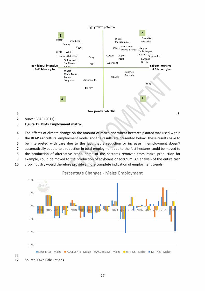
27
S1
ource: BFAP (2011) 2
Figure 19: BFAP Employment matrix 3
The effects of climate change on the amount of maize and wheat hectares planted was used within 4
the BFAP agricultural employment model and the results are presented below. These results have to 5
be interpreted with care due to the fact that a reduction or increase in employment doesn’t 6
automatically equate to a reduction in total employment due to the fact hectares could be moved to 7
the production of alternative crops. Some of the hectares removed from maize production for 8
example, could be moved to the production of soybeans or sorghum. An analysis of the entire cash 9
crop industry would therefore provide a more complete indication of employment trends. 10
11 Source: Own Calculations 12

28
Figure 20: Percentage Changes - Maize Employment 1
Again the largest impacts were calculated under the MPI 4.5 Scenario, with up to ten percent 2
variations in employment, both negative and positive. As explained in the above section, the 3
assumption will have to be made that these hectares are not replaced by another commodity. 4
5 Source: Own Calculations 6 Figure 21: Percentage Changes - Wheat Employment 7
8
Table 7: Compounded annual growth rates in employment 9
Compounded Annual Growth Rate
CAGR (2014-2025)
LTAS BASE - Maize -2.0%
ACCESS 4.5 - Maize -1.8%
ACCESS 8.5 - Maize -2.1%
MPI 8.5 - Maize -2.3%
MPI 4.5 - Maize -1.1%
LTAS BASE - Wheat -1.1%
ACCESS 4.5 - Wheat -1.0%
ACCESS 8.5 - Wheat -1.1%
MPI 8.5 - Wheat -1.2%
MPI 4.5 - Wheat -2.2%
Source: Own Calculations 10
In terms of maize production the results show the greatest expected decline (-2%) in base scenario 11
whereas the least favourable MPI 4.5 scenario shows the smallest decline (-1.1%) due to the 12
expansion on the area planted in response to the increase in price. Conversely the MPI 4.5 scenario 13
shows double (-2.2%) the decline in employment in terms wheat production (Table 7). 14
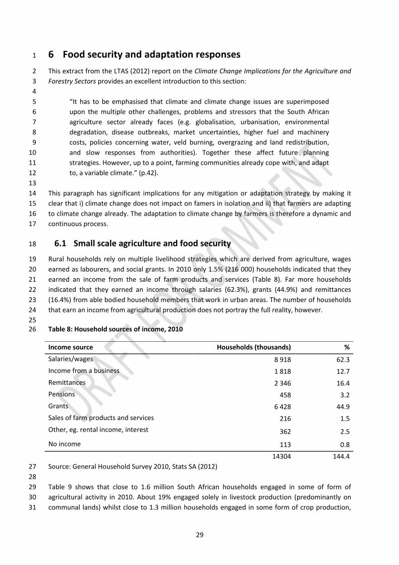
29
6 Food security and adaptation responses 1
This extract from the LTAS (2012) report on the Climate Change Implications for the Agriculture and 2
Forestry Sectors provides an excellent introduction to this section: 3
4
“It has to be emphasised that climate and climate change issues are superimposed 5
upon the multiple other challenges, problems and stressors that the South African 6
agriculture sector already faces (e.g. globalisation, urbanisation, environmental 7
degradation, disease outbreaks, market uncertainties, higher fuel and machinery 8
costs, policies concerning water, veld burning, overgrazing and land redistribution, 9
and slow responses from authorities). Together these affect future planning 10
strategies. However, up to a point, farming communities already cope with, and adapt 11
to, a variable climate.” (p.42). 12
13
This paragraph has significant implications for any mitigation or adaptation strategy by making it 14
clear that i) climate change does not impact on famers in isolation and ii) that farmers are adapting 15
to climate change already. The adaptation to climate change by farmers is therefore a dynamic and 16
continuous process. 17
6.1 Small scale agriculture and food security 18
Rural households rely on multiple livelihood strategies which are derived from agriculture, wages 19
earned as labourers, and social grants. In 2010 only 1.5% (216 000) households indicated that they 20
earned an income from the sale of farm products and services (Table 8). Far more households 21
indicated that they earned an income through salaries (62.3%), grants (44.9%) and remittances 22
(16.4%) from able bodied household members that work in urban areas. The number of households 23
that earn an income from agricultural production does not portray the full reality, however. 24
25 Table 8: Household sources of income, 2010 26
Income source Households (thousands) %
Salaries/wages 8 918 62.3
Income from a business 1 818 12.7
Remittances 2 346 16.4
Pensions 458 3.2
Grants 6 428 44.9
Sales of farm products and services 216 1.5
Other, eg. rental income, interest 362 2.5
No income 113 0.8
14304 144.4
Source: General Household Survey 2010, Stats SA (2012) 27
28
Table 9 shows that close to 1.6 million South African households engaged in some of form of 29
agricultural activity in 2010. About 19% engaged solely in livestock production (predominantly on 30
communal lands) whilst close to 1.3 million households engaged in some form of crop production, 31

30
mostly on small plots with 83.9% indicating that they produced on an area smaller than 0.5 hectares. 1
2 Table 9: South African households’ access to agricultural land, 2010 3
Agricultural Activity Households % in category % share in total
Crop production land size
Less than 0.5 1,073,888 83.8 67.7
Between 0.5 – 1 146,476 11.4 9.2
Between 1 – 2 47,402 3.7 3.0
Between 2 – 5 11,271 0.9 0.7
Between 5 -10 1,481 0.1 0.1
Between 10-20 246 0.0 0.0
1,280,764 100.0 80.8
Grazing
Communal Grazing (Livestock) 304,919 100.0 19.2
Total 1,585,683
100.0
Source: General Household Survey 2010, Stats SA (2012) compiled by Pienaar (2013) 4
5
When asked why they produce 86.8% indicated that they did so for an extra source of food, whilst 6
only 5.3% indicated that it serves as a main source of food, 4.5% as an additional source of income 7
and less than 1% as a primary source of income, as shown inFigure 22. Just under 94% of 8
respondents indicated that they do not sell agricultural produce. 9
10
SS11 Source: General Household Survey 2010, Stats SA (2012) compiled by Pienaar (2013) 12
Figure 22: Reason for engaging in Agriculture 13
Aliber (2009) showed there has been a strong movement since 2000 away from agricultural 14
production as a primary source of food and income toward agriculture as an additional source of 15

31
food and to a lesser extent as a source of income. This shift can be partly attributed to the expansion 1
of social grants, which seem to have replaced agricultural production as the primary rural livelihood 2
asset/safety net. The study also showed that agricultural production was mainly practiced by women 3
over the age of 50, which explains the fact that most households engage in agricultural production 4
as extra source of food. All able bodied persons therefore chose to seek urban employment. 5
6
One of the main adaptation responses to climate change is that of migration. Research in Africa in 7
recent decades showed that populations in rural areas have adopted strategies to cope with 8
recurring drought that incorporate migration. In Western Sudan, for example, male household 9
members have often migrated to Khartoum in search of wage labour when times of low rainfall 10
hinder agricultural production (Afolayan and Adelekan, 1998).In the dry-land production areas of 11
Ethiopia, migration is undertaken by families during times of drought after other measures such as 12
reducing food consumption and selling off possessions have been exhausted (Meze-Hausken, 2000). 13
This was also the case during the large-scale famines of the 1980s, where a considerable number of 14
households in northern Ethiopia migrated to the cities (Ezra, 2001). A study in Burkina Faso, 15
however, showed that land degradation has a greater influence over migration behaviour than 16
episodic climate-related events (Henry et al., 2004). 17
18
From a small scale/subsistence perspective agricultural activity in South Africa therefore does not 19
serve as primary source of subsistence but rather serves as a livelihood asset/safety net for the rural 20
poor when other income sources fall away (Tregurtha et al., 2009) or as supplement to existing 21
means. Given the above, a mass migration from rural to urban areas is not expected due to the fact 22
that most able bodied persons are already seeking employment beyond small scale agricultural 23
production. A reduction in the productivity of a small scale farmers will have the biggest impact on 24
the ability of households to supplement their consumption basket with additional food production. 25
This possible reduction will have to be mitigated through an expansion of existing grants, more 26
remittances etc. in order to enable additional food purchases. From a crop production perspective 27
these households could also be supported through the development of irrigation infrastructure and 28
extension tailored towards conservation and climate smart production systems. The removal of 29
supplementary food production in rural areas will put existing and often lacking transport 30
infrastructure under increased pressure. It is therefore essential that rural road infrastructure is 31
improved in order to ensure the delivery of food to rural areas at the lowest possible cost. This 32
improved infrastructure will also connect small scale producers to markets, which could increase 33
their income earned from agricultural production. 34
6.2 Continual adaptation and technology 35
This is illustrated by Case study 2 and figure 3, which have shown that farmers in traditional wheat 36
growing areas of the Free State province have stopped to produce due to a number consecutive 37
droughts and volatile price exposure. Farmers and seed companies are continually testing current 38
and new seed varieties through formal and informal field trials in order to ensure that the best 39
suited varieties. These trials enable the identification of the best suited variety for the specific region 40
or farm, given the unique and possibly changing attributes of each given rainfall, temperature, 41
daylight length etc. 42
43
Significant progress has been made by seed companies with improved hybrid varieties. One example 44

32
is the development of drought resistant genetically modified maize varieties such as the registration 1
of the DroughtGuard® technology by Monsanto in US in December 2011. The company claims a 5 2
bushel per acre (approx. 300 kg/ha) advantage above other drought tolerant varieties (Monsanto, 3
2014). This have not been very well received throughout, however, with the Union for Concerned 4
Scientists (UCS) claiming that it only “…provides only modest results in only moderate drought 5
conditions” (Gillam, 2012). 6
7
Farmers are also employing other adaptation/mitigation strategies in order to reduce their 8
production risk. This includes the planting of varieties with a shorter growing period, delaying the 9
start of planting in accordance to rainfall, investments in more machinery in order to shorten 10
planting time, the collection of rain water through the creation of furrows near plants and increased 11
use of irrigation (Benhin, 2006). Small scale crop farmers are being encouraged by AgriSA to adopt 12
improved farm management practices, especially in terms of the timing of planting and tillage 13
practices. Farmers, both small scale and commercial, are increasingly adopting conservation tillage 14
practices due to the advantages of reduced soil moisture losses, weed control, reduced erosion and 15
increased general soil health and climate smart agriculture approaches are being advocated by DAFF 16
which include conservation tillage approaches . 17
6.3 Irrigation 18
Irrigation is of the central themes when considering climate change, agriculture and adaptation. At 19
present the agricultural sector consumes 60% of the available water for irrigation (Blignaut et al., 20
2009). Map 2 shows the various South African water management areas as presented in the National 21
Water Resource Strategy 2004. According to this report water management areas 4, 5. 7 and 11 are 22
already over utilising available water mainly due to significant industrial and residential usage in 23
these areas. Excess water is currently available in water management areas 6, 12, 15 (all on the 24
eastern seaboard) and 15 (upper Orange) (DWA, 2004). It is estimated that an additional area of 90 25
000 ha could be added without an investment in additional storage capacity and more than 300 000 26
hectares could potentially be added through investments in additional capacity (BFAP, 2011). Note 27
that all of management areas with available water do not include major urban settlements or 28
industrial areas and thus a large percentage of the water could be utilised for agricultural 29
production. 30
31
A major source of additional water, especially relevant within the context of a drying climate, is that 32
of possible efficiency gains. The technical efficiency of different types of irrigation differs significantly 33
‒ flood irrigation achieves 55-65%, compared to 75-85% for sprinkler irrigation and 85-95% for 34
micro-irrigation systems. The extent to which each of these is prevalent in South Africa is shown in 35
Table 10. It shows that a total of just over 1.6 million hectares were irrigated in 2007 of which the 36
largest percentage was irrigated through sprinkler systems. The switch to micro-irrigation systems 37
has been slow ‒ increasing from 11.8% to 21.8% in almost two decades (Backeberg and Reinders, 38
2009). 39

33
S1
ource: DWA, (2004) 2
Map 2: South African Water Management Areas 3
4
It can be assumed that the remaining area under flood irrigation could be converted to the 5
alternative systems, preferably micro and drip for horticultural products and centre pivots for grains, 6
oilseeds, given sufficient incentives to do so. The usage of this system should also be encouraged 7
with future expansion. An additional source of efficiency gains is possible through the improved 8
maintenance and upgrading of existing infrastructure, especially channels, and the implementation 9
of a water management system (WAS). The implementation of a WAS in the Loskop (Mpumalanga) 10
and Orange-Riet (Northern Cape) rivers resulted in a 50% reduction in losses, 30-40% to 15-20%. The 11
conversion to more efficient modes of irrigation and the implementation of a national WAS could 12
result in expansion of the area under irrigation by an additional 282 000 hectares (BFAP, 2011), given 13
current water availability levels. 14
15
Table 10: Agricultural irrigation: Area and Method 16
Irrigation method (%)
Area (ha) Flood Sprinkler Micro/Drip
1990 1,290,132 33 54 11.8
2007 1,675,882 14.5 54.9 21.8
Source: (Backeberg and Reinders, 2009) 17
18
6.4 Expansion of area planted 19
South Africa currently utilises about 13m ha of agricultural land for field crop and horticultural 20
production, while total land cultivation was as high as 16.2m ha in the 1980s. The reduction in this 21

34
area is the removal of marginal land from production after the removal of agricultural price support 1
schemes from the late 1980s to late 90s. These fields were removed due to unsuitable gradients, 2
unfavourable soil properties and to low rainfall. At present the amount of arable land is estimated at 3
15m hectares, this includes some land previously cultivated and underutilised land in former 4
homeland areas. Some of the land previously cultivated could be reintroduced into production given 5
an increase in real net revenue per hectare. This is confirmed by the BFAP sector model that 6
indicates an increase in the area planted under maize of more than 200 000 ha under the MPI 4.5 7
scenario. The decline in yields due to lower precipitation is offset by an increase in market prices due 8
to lower production levels, therefore net revenue increases and farmers expand the area under 9
production. According to the BFAP sector model, the total area under the main grain and oilseeds is 10
projected to find its long-run equilibrium around 4.2 million hectares by 2020, compared to 4.4 11
million hectares in 2014 and 6.7 million hectares in 1980. . 12
7 High-level messages and Policy recommendations 13
This study investigated the effects of the respective climate change scenarios identified in the LTAS 1 14
project on South African maize and wheat industries from an economic, food security and 15
employment perspective for the period 2014 to 2030. This was achieved through including 16
precipitation data generated from various climate models that best suit each of the LTAS 1 scenarios 17
in the BFAP sector model. 18
19
Towards 2030 the results of the analysis showed that is imperative that the results of the respective 20
scenarios are only interpreted after a careful consideration of major trends in the base scenario. This 21
analysis showed the area under white maize production is expected to decline in response flat 22
domestic demand in conjunction with a yearly increase in yield. Prices are expected to remain at 23
export parity levels. Within this context farms opt to increase the area under soybean production in 24
response to price signals, increased yield and domestic demand. Yellow maize area under production 25
is expected show small increase whilst yields show a yearly increase and prices remain at export 26
parity levels. The area under wheat production is expected to show a small decrease in favour of the 27
production of alternative crops, mainly canola. Net imports are expected to decline due to the 28
combination of decreasing production and increasing demand. 29
30
From a climate perspective the worst climate scenario, warmer/moderately drier (MPI 4.5) is 31
anticipated to decrease the average white maize yield by more than tonne per hectare. This results 32
in an increase in prices that induce a smaller decline in the area under production than the base 33
scenario. As stated in Section 6.2 the challenges faced due to climate change does not act on 34
producers in isolation but rather forms part of the bigger collective challenges. Any adaptation 35
strategy should therefore be guided by this econometrically integrated view, and not based solely on 36
the biophysical impacts on the crop yield itself. Adaptation strategies also require consideration of 37
specific groups of producers, i.e. small scale or commercial, so that options sought are scale neutral 38
and beneficial to the industry regardless of which climate scenario materialises. Example strategies 39
that meet this criterion include improved transport infrastructure, improvements in irrigation 40
efficiency and water management, coordinated field trials in partnership between farmers, private 41
companies and the state as discussed below. 42
43
It also has to be reiterated that farmers are already adapting to climate change. The observed 44
35
historic reduction in the area under wheat production serves as a good example. Farmers have 1
opted to decrease the area planted by more than half, partly in response to price decreases but also 2
in order to decrease exposure to climate risk such as too low or rainfall during harvest. Farmers are 3
also continually doing formal and informal field trials in order to identify the best suited varieties for 4
each locality. The role foreseen for the public sector is not replace these initiatives but rather to 5
support, expand and integrate the results of these respective trials. Greater cooperation between 6
the farmers, seed companies and state will improve the focus of public research and improve quality 7
of extension services provided, particularly for small scale farmers in close proximity of these trials. 8
9
This study showed that the area under irrigation can be expanded through new investments in 10
storage capacity. Significant gains are possible, however, within existing systems through decreases 11
in distribution loses, the adoption of more efficient irrigation systems and improvements in 12
management of existing irrigation systems. This has the potential to add an additional area of 282 13
000 hectares under production, simply by using available water. The maintenance of and 14
improvements to existing irrigation systems is therefore imperative. Incentives for the upgrading of 15
existing systems to more efficient alternatives, for example flood irrigation to drip, should be 16
provided by the state, alternatively the amount of water available to consumers should be regulated 17
in order to warrant investments in more efficient systems. 18
19
South Africa has been a net importer of wheat since the early 1990s but also experienced significant 20
increases in agricultural exports since. According to the MPI 4.5 climate scenario wheat imports are 21
expected to increase substantially due to a decline in production and increase in consumer demand 22
for wheat. Increasingly larger amounts of wheat will therefore have to be moved between sources of 23
supply or the respective ports, and sources of demand. A cost efficient transport system is therefore 24
an imperative in order to ensure the provision of this staple at the lowest possible cost. An 25
improvement in port, rail and road infrastructure is therefore of utmost importance, especially 26
railways. Inversely this infrastructure will also improve the competitiveness of agricultural exports, 27
particularly fruit and wine. These exports as significant earners of foreign exchange currently and 28
will continue to “afford” the substantial and growing primary food stuff imports. The exports of 29
these products will have to be expanded in future in order to maintain a positive agricultural trade 30
balance and avoid the negative effects of exchange deficits. This also includes the improvement of 31
SADC regional road and rail networks in order to enable more cost efficient trade. Zimbabwe is 32
currently one of South Africa’s biggest trade partners. Fruit and wine exports to SADC is expect 33
continue to grow whist Zambia could serve as important trade partner for wheat for example. 34
35
Transport infrastructure is not limited to harbour, rail and main roads, however, and a significant 36
number of (mostly rural) households have access to land and a large percentage of them engage in 37
agricultural production as an additional source of food and to lesser extent as an additional source of 38
income. It is possible, however, that some of climate scenarios could decrease the ability of 39
households to engage in agricultural production as an additional source of food. This would result in 40
an increased need for food shipments to rural areas to address this deficit, which would put existing 41
(mostly poor) rural roads under further pressure. It is therefore advised that these rural roads should 42
be maintained to increase the efficiency of transported food items to these rural areas. This 43
improved infrastructure could likewise increase small scale farmers’ ability to engage in agricultural 44
production for income purpose through connecting them to sources of demand. 45
36
8 Future research needs with links to future adaptation work and 1
modelling capacity 2
This study has provided an essential first perspective but it is only a limited one. Maize and wheat 3
are only part of a bigger production system wherein producers are continuously making adjustments 4
to the allocation of their resources in order to maximise the return to their labour and capital. A 5
study that follows an integrated approach to a much larger number of commodities is therefore 6
needed. The expected trend in expanded soybean and canola production serves as a good example 7
of shits not reflected in this study. 8
9
One of the major trends identified is that of a continuation of the increase in wheat imports, a trend 10
that will be accelerated within some of the climate scenarios. The sector have been able maintain a 11
positive agricultural trade balance despite the increase in wheat and other imports, mainly due to 12
the strong growth in fruit and wine exports. A failure to maintain a positive trade balance will result 13
in depreciation of the Rand that in turn will result in increases in the prices of the large and growing 14
amounts of imported wheat (and rice of which 100% is imported). Ultimately reduce access to food 15
due to reduced affordability. 16
17
The fruit and wine sectors are perceived to be under greater risk from climate change due to their 18
sensitivity to temperature increases. Future research on the climate impacts on these crops is 19
therefore very important. Various strategies directed towards the expansion of the competitiveness 20
of these industries are an essential adaptation strategy and a topic also in need of future research. 21
The narrow focus of current research on maize and wheat production may be a result of a conflation 22
of food security and food self-sufficiency. Given the current imports of wheat, the inability to 23
increase production and the expected increase in demand puts self-sufficiency clearly of the table. 24
An integrated approach to the availability and affordability aspects of food is therefore much needed 25
in future research. 26
27

37
References 1
Afolayan, A. & Adelekan, I. (1998) The role of climatic variations on migration and human 2
health in Africa. Environmentalist. 18213–218. 3
Backeberg, G. R. & Reinders, F. B. (2009) 'Institutional Reform and Modernisation of 4
Irringation Systems in South Africa', in 5th Asian Regional Conference of ICID. 2009 New 5
Delhi: . 6
Benhin, J. (2006) Climate change and South African agriculture: Impacts and adaptation 7
options. (21). 8
BFAP (2011) The Contribution of the Agro-Industrial Complex to Employment in South Africa. 9
(June) p.44. 10
Blignaut, J. et al. (2009) Agriculture Production’s Sensitivity to Changes in Climate in South 11
Africa. South African Journal of Science. 105 (January/February), 61–68. 12
DAS (2013) Abstract of agricultural statistics. Pretoria: Directorate of Agricultural Statistics, 13
South Africa. 14
DWA (2004) National Water Resource Strategy. 15
Estes, L. D. et al. (2013) Projected climate impacts to South African maize and wheat 16
production in 2055: A comparison of empirical and mechanistic modeling approaches. 17
Global change biology. [Online] 19 (12), 3762–3774. 18
Ezra, M. (2001) Demographic responses to environmental stress in the drought- and famine-19
prone areas of northern Ethiopia. International Journal of Population Geography. 20
[Online] 7 (4), 259–279. 21
Gillam, C. (2012) Science group finds drought-tolerant GMO corn lacking [online]. Available 22
from: http://www.reuters.com/article/2012/06/05/corn-monsanto-23
idUSL1E8H4JMW20120605 (Accessed 17 April 2014). 24
Hachigonta, S. et al. (2013) Southern African Agriculture and Climate Change. Washington, 25
D.C.: International Food Policy Research Institute. 26
Henry, S. et al. (2004) Descriptive analysis of the individual migratory pathways according to 27
environmental typologies. Population and Environment. 25 (5), 397–422. 28
LTAS (2013) Climate Change Implications for the Agriculture and Forrestry Sectors in South 29
Africa. 30
Meze-Hausken, E. (2000) Migration caused by climate change: how vulnerable are people 31
inn dryland areas? Mitigation and Adaptation Strategies for Global Change. 5379–406. 32

38
Monsanto (2014) Genuity® | DroughtGard® Hybrids. A Systems Approach to Manage 1
Drought [online]. Available from: http://www.genuity.com/corn/Pages/Genuity-2
DroughtGard-Hybrids.aspx (Accessed 22 April 2014). 3
Nel, J. H. & Steyn, N. P. (2002) Report on South African Food Consumption Studies 4
Undertaken amongst Different Population Groups. 5
Nelson, G. et al. (2010) Food security, farming, and climate change to 2050: Scenarios, 6
results, policy options. Washington, D.C.: International Food Policy Research Institute. 7
Nelson, G. C. et al. (2009) Climate Change Impact on Agriculture and Costs of Adaptation. 8
Washington, D.C.: International Food Policy Research Insitute. 9
Oldewage-Theron, W. H. et al. (2005) A community-based integrated nutrition research 10
programme to alleviate poverty: baseline survey. Public health. 119 (4), 312–320. 11
Pienaar, P. L. (2013) Typology of Smallholder Farming in South Africa’s Former Homelands: 12
Towards an Appropriate Classification System. Stellenbosch University. 13
Ringler, C. et al. (2010) Climate Change Impacts on Food Security in Sub-Saharan Africa 14
Insights from Comprehensive Climate Change Scenarios. (December), . 15
SAGIS (2013) Commodity Statistics. Pretoria: South African Grain Information Service. 16
Stats SA (2012) General Household Survey. 2010 (July 2011) p.156. 17
StatsSA (2012) Expenditure Survey Income and Expenditure of Households 2010/2011. 18
Steyn, N. et al. (2000) The National Food Consumption Survey (NFCS): Children aged 1-9 19
years, South Africa, 1999. 20
Tregurtha, N. et al. (2009) Presidency Fifteen Year Review Project. Africa (November 2009). 21
Vink, N. & Kirsten, J. (2000) Deregulation of Agricultural Marketing in South Africa. p.45. 22
23

39
Annexes
Annexure A: The BFAP Poor person’s index – Projected results
2013 2014 2015 2016 2017 2018 2019 2020 2021 2022 2023 2024 2025
Base: Total cost of 5 items (Index with
2013=100) 100 103 106 110 113 117 119 124 127 131 134 139 143
Scenario MPI4.5: Total cost of 5 items
(Index with 2013=100) 100 105 110 112 117 119 123 128 128 135 139 143 146
Percentage increase 0.0% 1.7% 3.3% 1.8% 3.4% 1.4% 3.1% 3.2% 1.2% 3.0% 3.5% 2.9% 1.9%
Annexure B: The BFAP Poor person’s index – Projected results based on the cost share contributions of maize meal and bread within the portion-weighed
five item food plate
2013 2014 2015 2016 2017 2018 2019 2020 2021 2022 2023 2024 2025
%
Base: Maize as share of total cost
28.8 27.8 26.9 27.5 26.9 27.4 26.4 27.2 26.3 26.6 26.2 26.2 26.3
Scenario MPI 4.5: Maize as share of total cost
28.8 29.0 29.2 28.7 29.3 28.4 28.6 29.5 27.2 28.7 28.7 28.3 27.6
Base: Brown bread as share of total cost
44.7 46.5 48.2 48.5 49.6 50.0 51.4 51.5 52.7 53.1 54.1 54.7 55.2
Scenarion MPI 4.5: Brown bread as share of total cost
44.7 45.8 46.7 47.7 48.0 49.3 49.8 49.9 52.1 51.6 52.2 53.1 54.2

40
Annexure C: The potential additional expenditure on maize meal and bread if consumption quantities remain the same (2010) at higher price levels:
ID 1 ID 2 ID 3 ID 4 ID 5 ID 6 ID 7 ID 8 ID 9 ID 10
1. Maize meal expenditure in 2010
(R/hh/year) R 614 R 893 R 947 R 969 R 914 R 751 R 658 R 553 R 341 R 180
2. Estimated maize meal expenditure at
projected BASE price max level (R/hh/year) R 1,255 R 1,824 R 1,936 R 1,980 R 1,869 R 1,536 R 1,344 R 1,130 R 698 R 368
3. Estimated maize meal expenditure at
projected CLIMATE CHANGE SCENARIO
price max level (R/hh/year)
R 1,345 R 1,955 R 2,076 R 2,122 R 2,003 R 1,646 R 1,441 R 1,211 R 748 R 395
Difference (scenarion less base)
(R/hh/year) [(3) less (2)] R 90 R 131 R 139 R 142 R 134 R 110 R 97 R 81 R 50 R 26
Difference (scenarion less base)
(R/hh/month) R 7.52 R 10.93 R 11.60 R 11.86 R 11.20 R 9.20 R 8.05 R 6.77 R 4.18 R 2.21
Diff as share of 2010 income levels 1.9% 1.0% 0.7% 0.5% 0.4% 0.2% 0.1% 0.1% 0.0% 0.0%
Diff as share of projected 2025 income
levels 1.1% 0.6% 0.4% 0.3% 0.2% 0.1% 0.1% 0.0% 0.0% 0.0%

41
Annexure D: The potentially reduced energy intake if staple food budgets remain unchanged at 2010 levels but retail prices of bread and maize meal
increases as per projections.
ID 1 ID 2 ID 3 ID 4 ID 5 ID 6 ID 7 ID 8 ID 9 ID 10
1. Energy value contribution of maize meal in 2010 (kJ per
household member per day) 2,446 2,515 2,350 2,477 2,066 1,734 1,535 1,308 822 447
2. Energy contribution of maize meal acc to maxiumum
projected 'base' price (kJ per household member per day) 1,197 1,231 1,150 1,212 1,011 848 751 640 402 219
3. Energy contribution of maize meal acc to maxiumum
projected 'climate change scenario' price (kJ per household
member per day)
1,116 1,148 1,073 1,130 943 791 701 597 375 204
Difference (kJ/ household member/day) [(3) less (2)] -80 -83 -77 -81 -68 -57 -50 -43 -27 -15