caso placa 4
TRANSCRIPT

8/10/2019 Caso Placa 4
http://slidepdf.com/reader/full/caso-placa-4 1/42
CIVL 7117 Finite Elements Methods in Structural Mechanics Page 244
Development of the Plane Stress and PlaneStrain Stiffness Equations
Introduction
In Chapters 2 through 5, we considered only line elements. Line elements are
connected only at common nodes, forming framed or articulated structures such
as trusses, frames, and grids. Line elements have geometric properties such as
cross-sectional area and moment of inertia associated with their cross sections.
However, only one local coordinate along the length of the element is required to
describe a position along the element (hence, they are called line elements).
Nodal compatibility is then enforced during the formulation of the nodal
equilibrium equations for a line element.
This chapter considers the two-dimensional finite element. Two-dimensional
(planar) elements are thin-plate elements such that two coordinates define a
position on the element surface.
The elements are connected at common nodes and/or along common edges
to form continuous structures. Nodal compatibility is then enforced during the
formulation of the nodal equilibrium equations for two-dimensional elements. If
proper displacement functions are chosen, compatibility along common edges is
also obtained.
8/10/2019 Caso Placa 4
http://slidepdf.com/reader/full/caso-placa-4 2/42
CIVL 7117 Finite Elements Methods in Structural Mechanics Page 245
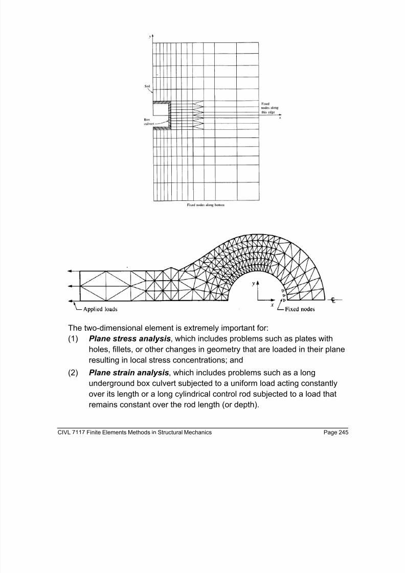
The two-dimensional element is extremely important for:
(1) Plane stress analysis, which includes problems such as plates with
holes, fillets, or other changes in geometry that are loaded in their planeresulting in local stress concentrations; and
(2) Plane strain analysis, which includes problems such as a long
underground box culvert subjected to a uniform load acting constantly
over its length or a long cylindrical control rod subjected to a load that
remains constant over the rod length (or depth).

8/10/2019 Caso Placa 4
http://slidepdf.com/reader/full/caso-placa-4 3/42
CIVL 7117 Finite Elements Methods in Structural Mechanics Page 246
Plane Stress Problems
Plane Strain Problems
We begin this chapter with the development of the stiffness matrix for a basic
two-dimensional or plane finite element, called the constant-strain triangular
element . The constant-strain triangle (CST) stiffness matrix derivation is the
simplest among the available two-dimensional elements.We will derive the CST stiffness matrix by using the principle of minimum
potential energy because the energy formulation is the most feasible for the
development of the equations for both two- and three-dimensional finite
elements.
8/10/2019 Caso Placa 4
http://slidepdf.com/reader/full/caso-placa-4 4/42
CIVL 7117 Finite Elements Methods in Structural Mechanics Page 247
General Steps in the Formulation of the Plane Triangular Element
Equations
We will now follow the steps described in Chapter 1 to formulate the governing
equations for a plane stress/plane strain triangular element. First, we willdescribe the concepts of plane stress and plane strain. Then we will provide a
brief description of the steps and basic equations pertaining to a plane triangular
element.
Plane Stress
Plane stress is defined to be a state of stress in which the normal stress and
the shear stresses directed perpendicular to the plane are assumed to be zero.
That is, the normal stress σz and the shear stresses τ xz and τyz are assumed tobe zero. Generally, members that are thin (those with a small z dimension
compared to the in-plane x and y dimensions) and whose loads act only in the x-
y plane can be considered to be under plane stress.
Plane Strain
Plane strain is defined to be a state of strain in which the strain normal to the
x-y plane εz and the shear strains γ xz and γyz are assumed to be zero. The
assumptions of plane strain are realistic for long bodies (say, in the z direction)
with constant cross-sectional area subjected to loads that act only in the x and/or
y directions and do not vary in the z direction.
Two-Dimensional State of Stress and Strain
The concept of two-dimensional state of stress and strain and the stress/strain
relationships for plane stress and plane strain are necessary to understand fully
the development and applicability of the stiffness matrix for the plane
stress/plane strain triangular element.
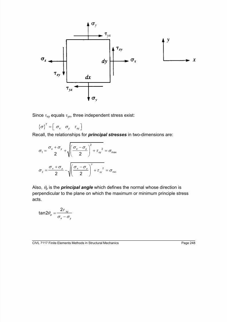
A two-dimensional state of stress is shown in the figure below. The
infinitesimal element with sides dx and dy has normal stresses σz and σy acting in
the x and y directions (here on the vertical and horizontal faces), respectively.
The shear stress τ xy acts on the x edge (vertical face) in the y direction. The
shear stress τyx acts on the y edge (horizontal face) in the x direction.
8/10/2019 Caso Placa 4
http://slidepdf.com/reader/full/caso-placa-4 5/42
CIVL 7117 Finite Elements Methods in Structural Mechanics Page 248
Since τ xy equals τyx , three independent stress exist:
T
x y xy σ σ σ τ =
Recall, the relationships for principal stresses in two-dimensions are:
σ σ σ σ σ τ σ + − = + + =
2
21 max
2 2 x y x y
xy
min
2
2
222
σ τ σ σ σ σ
σ =+
−−
+=
xy
y x y x
Also, θ p is the principal angle which defines the normal whose direction is
perpendicular to the plane on which the maximum or minimum principle stress
acts.
2tan2
xy
p
x y
τ θ
σ σ =
−

8/10/2019 Caso Placa 4
http://slidepdf.com/reader/full/caso-placa-4 6/42
CIVL 7117 Finite Elements Methods in Structural Mechanics Page 249
The general two-dimensional state of strain at a point is show below.
The general definitions of normal and shear strains are:
x
v
y
u
x
v
x
u xy y x ∂
∂+
∂∂
=∂∂
=∂∂
= γ ε ε
The strain may be written in matrix form as:
T
x y xy ε ε ε γ =
8/10/2019 Caso Placa 4
http://slidepdf.com/reader/full/caso-placa-4 7/42
CIVL 7117 Finite Elements Methods in Structural Mechanics Page 250
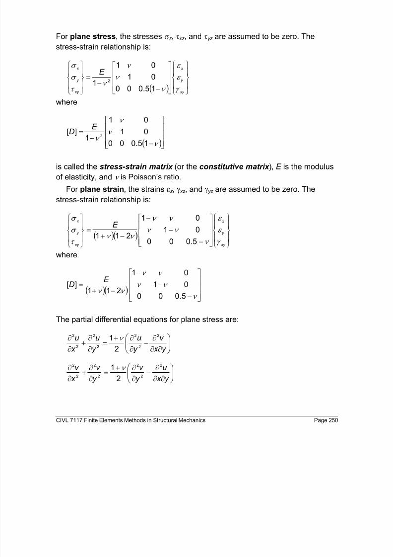
For plane stress, the stresses σz , τ xz , and τyz are assumed to be zero. The
stress-strain relationship is:
( )
−−
=
xy
y
x
xy
y
x
E
γ
ε
ε
ν
ν
ν
ν τ
σ
σ
15.000
01
01
12
where
( )
−−
=
ν
ν
ν
ν 15.000
01
01
1][
2
E D
is called the stress-strain matrix (or the constitutive matrix ), E is the modulus
of elasticity, and ν is Poisson’s ratio.
For plane strain, the strains εz , γ xz , and γyz are assumed to be zero. The
stress-strain relationship is:
( )( )
−
−
−
−+=
xy
y
x
xy
y
x
E
γ
ε
ε
ν
ν ν
ν ν
ν ν τ
σ
σ
5.000
01
01
211
where
( )( )
−
−
−
−+=
ν
ν ν
ν ν
ν ν 5.000
01
01
211][
E D
The partial differential equations for plane stress are:
∂∂
∂−∂
∂+=∂
∂+∂
∂y x
v
y
u
y
u
x
u 2
2
2
2
2
2
2
2
1 ν
∂∂
∂−
∂∂+
=∂∂
+∂∂
y x
u
y
v
y
v
x
v 2
2
2
2
2
2
2
2
1 ν
8/10/2019 Caso Placa 4
http://slidepdf.com/reader/full/caso-placa-4 8/42
CIVL 7117 Finite Elements Methods in Structural Mechanics Page 251
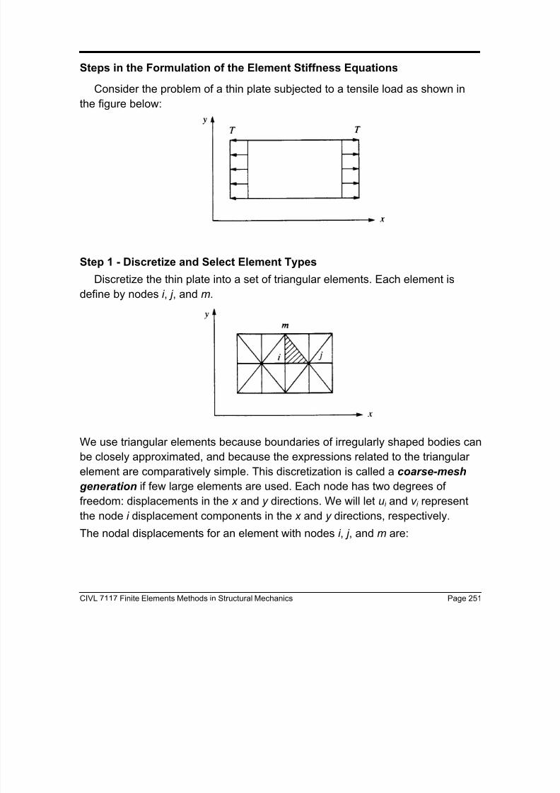
Steps in the Formulation of the Element Stiffness Equations
Consider the problem of a thin plate subjected to a tensile load as shown in
the figure below:
Step 1 - Discretize and Select Element Types
Discretize the thin plate into a set of triangular elements. Each element is
define by nodes i , j , and m.
We use triangular elements because boundaries of irregularly shaped bodies can
be closely approximated, and because the expressions related to the triangular
element are comparatively simple. This discretization is called a coarse-mesh
generation if few large elements are used. Each node has two degrees offreedom: displacements in the x and y directions. We will let ui and v i represent
the node i displacement components in the x and y directions, respectively.
The nodal displacements for an element with nodes i , j , and m are:
8/10/2019 Caso Placa 4
http://slidepdf.com/reader/full/caso-placa-4 9/42
CIVL 7117 Finite Elements Methods in Structural Mechanics Page 252
=
m
j
i
d
d
d
d
where the nodes are ordered counterclockwise around the element, and
=
i
i
i v ud
Therefore:
=
m
m
j
j
i
i
v
u
v
u
v
u
d
Step 2 - Select Displacement Functions
The general displacement function is:
=Ψ),(
),(
y x v
y x ui
The functions u( x, y ) and v ( x, y ) must be compatible with the element type.
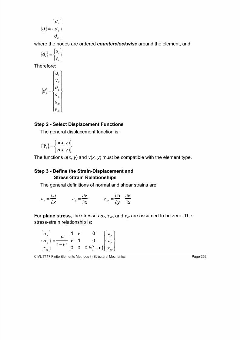
Step 3 - Define the Strain-Displacement and
Stress-Strain Relationships
The general definitions of normal and shear strains are:
x
v
y
u
x
v
x
u xy y x ∂
∂+
∂∂
=∂∂
=∂∂
= γ ε ε
For plane stress, the stresses σz , τ xz , and τyz are assumed to be zero. The
stress-strain relationship is:
( )
−−
=
xy
y
x
xy
y
x
E
γ
ε
ε
ν
ν
ν
ν τ
σ
σ
15.000
01
01
1 2

8/10/2019 Caso Placa 4
http://slidepdf.com/reader/full/caso-placa-4 10/42
CIVL 7117 Finite Elements Methods in Structural Mechanics Page 253
For plane strain, the strains εz , γ xz , and γyz are assumed to be zero. The
stress-strain relationship is:
( )( )
−
−
−
−+
=
xy
y
x
xy
y
x
E
γ
ε
ε
ν
ν ν
ν ν
ν ν τ
σ
σ
5.000
01
01
211
Step 4 - Derive the Element Stiffness Matrix and Equations
Using the principle of minimum potential energy, we can derive the element
stiffness matrix.
d k f ][=
This approach is better than the direct methods used for one-dimensional
elements.
Step 5 - Assemble the Element Equations and
Introduce Boundary Conditions
The final assembled or global equation written in matrix form is:
d K F ][=
where F is the equivalent global nodal loads obtained by lumping distributed
edge loads and element body forces at the nodes and [K ] is the global structure
stiffness matrix.
Step 6 - Solve for the Nodal Displacements
Once the element equations are assembled and modified to account for the
boundary conditions, a set of simultaneous algebraic equations that can be
written in expanded matrix form as:
Step 7 - Solve for the Element Forces (Stresses)
For the structural stress-analysis problem, important secondary quantities of
strain and stress (or moment and shear force) can be obtained in terms of the
displacements determined in Step 6.
8/10/2019 Caso Placa 4
http://slidepdf.com/reader/full/caso-placa-4 11/42
CIVL 7117 Finite Elements Methods in Structural Mechanics Page 254
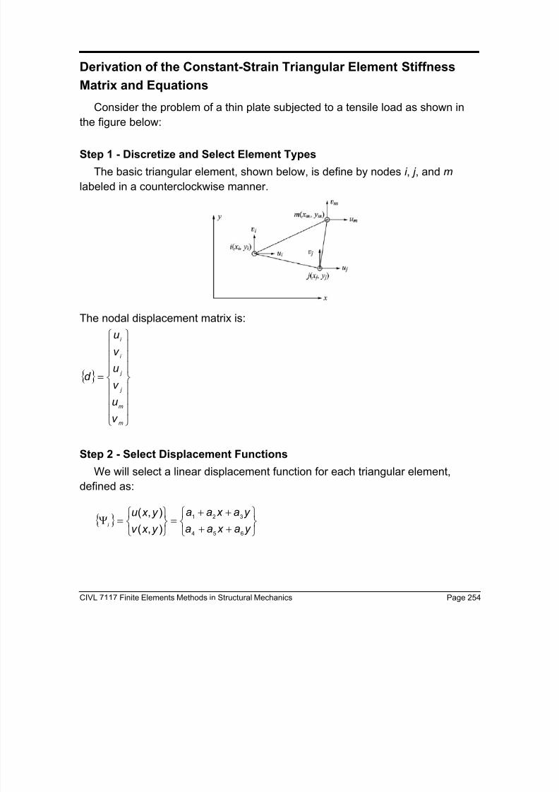
Derivation of the Constant-Strain Triangular Element Stiffness
Matrix and Equations
Consider the problem of a thin plate subjected to a tensile load as shown in
the figure below:
Step 1 - Discretize and Select Element Types
The basic triangular element, shown below, is define by nodes i , j , and m
labeled in a counterclockwise manner.
The nodal displacement matrix is:
=
m
m
j
j
i
i
v
u
v
u
v
u
d
Step 2 - Select Displacement Functions
We will select a linear displacement function for each triangular element,
defined as:
++
++=
=Ψy a x aa
y a x aa
y x v
y x ui
654
321
),(
),(

8/10/2019 Caso Placa 4
http://slidepdf.com/reader/full/caso-placa-4 12/42
CIVL 7117 Finite Elements Methods in Structural Mechanics Page 255
A linear function ensures that the displacements along each edge of the element
and the nodes shared by adjacent elements are equal.
=
++
++=Ψ
6
5
4
3
2
1
654
321
1000
0001
a
a
a
a
a
a
y x
y x
y a x aa
y a x aai
To obtain the values for the a’s substitute the coordinated of the nodal points into
the above equations:
i i i i i i y a x aav y a x aau
654321 ++=++=
j j j j j j y a x aav y a x aau
654321 ++=++=
mmmmmmy a x aav y a x aau
654321 ++=++=
Solving for the a’s and writing the results in matrix forms gives:
[ ] u x a
a
a
a
y x
y x
y x
u
u
u
mm
j j
i i
m
j
i
1
3
2
1
1
1
1−=⇒
=
(x j, y j)
(xi, yi) (xm, ym)
ui
u j
um
u
y
x
Linear representation of u(x, y)

8/10/2019 Caso Placa 4
http://slidepdf.com/reader/full/caso-placa-4 13/42
CIVL 7117 Finite Elements Methods in Structural Mechanics Page 256
The inverse of the [ x ] matrix is:
=−
m j i
m j i
m j i
A x
γ γ γ
β β β
α α α
2
1][ 1
where
mm
j j
i i
y x
y x
y x
A
1
1
1
2 =
is the determinant of [ x ].
( ) j i mi m j m j i y y x y y x y y x A −+−+−=2
where A is the area of the triangle and
j mi m j i m j m j i x x y y x y y x −=−=−= γ β α
mi j i m j mi mi j x x y y x y y x −=−=−= γ β α
i j m j i m j i j i m x x y y x y y x −=−=−= γ β α
The values of a may be written matrix form as:
=
m
j
i
m j i
m j i
m j i
u
u
u
Aa
a
a
γ γ γ
β β β
α α α
2
1
3
2
1
and
=
m
j
i
m j i
m j i
m j i
v
v
v
Aa
a
a
γ γ γ
β β β
α α α
2
1
6
5
4

8/10/2019 Caso Placa 4
http://slidepdf.com/reader/full/caso-placa-4 14/42
CIVL 7117 Finite Elements Methods in Structural Mechanics Page 257
We will now derive the displacement function in terms of the coordinates x and y .
[ ]
=
3
2
1
1
a
a
a
y x u
Substituting the values for a into the above equation gives:
[ ]1
12
i j m i
i j m j
i j m m
u
u x y u A
u
α α α
β β β
γ γ γ
=
Expanding the above equations
[ ]1
12
i i j j m m
i i j j m m
i i j j m m
u u u
u x y u u u Au u u
α α α
β β β γ γ γ
+ +
= + + + +
Multiplying the matrices in the above equations gives
( ) ( ) ( ) 1
( , )2
i i i i j j j j m m m mu x y x y u x y u x y u A
α β γ α β γ α β γ = + + + + + + + +
A similar expression can be obtained for the y displacement
( ) ( ) ( ) 1
( , )2
i i i i j j j j m m m mv x y x y v x y v x y v A
α β γ α β γ α β γ = + + + + + + + +
The displacements can be written in a more convenience form as:
mm j j i i mm j j i i v N v N v N y x v uN uN uN y x u ++=++= ),(),(
where
( ) ( ) ( )y x A
N y x A
N y x A
N mmmm j j j j i i i i
γ β α γ β α γ β α ++=++=++=21
21
21
The elemental displacements can be summarized as:
++
++=
=Ψmm j j i i
mm j j i i
i v N v N v N
uN uN uN
y x v
y x u
),(
),(

8/10/2019 Caso Placa 4
http://slidepdf.com/reader/full/caso-placa-4 15/42
CIVL 7117 Finite Elements Methods in Structural Mechanics Page 258
In another form the above equations are:
0 0 0
[ ] 0 0 0
i
i
i j m j
i j m j
m
m
u
v
N N N u
N d N N N v
u
v
ψ
Ψ = =
where
[ ]
=
m j i
m j i
N N N
N N N N
000
000
The linear triangular shape functions are illustrated below
Step 3 - Define the Strain-Displacement and Stress-Strain Relationships
Elemental Strains: The strains over a two-dimensional element are:
∂∂
+∂∂
∂∂∂∂
=
=
x
v
y
uy
v x u
xy
y
x
γ
ε
ε
ε
j
i m
1
N i
y
x
j
i m
1
N j
y
x
j
i m
1
N m
y
x

8/10/2019 Caso Placa 4
http://slidepdf.com/reader/full/caso-placa-4 16/42
CIVL 7117 Finite Elements Methods in Structural Mechanics Page 259
Substituting our approximation for the displacement gives:
( )mm j j i i x
uN uN uN x
u x
u++
∂∂
==∂∂
,
m x m j x j i x i x
uN uN uN u,,,,
++=
where the comma indicates differentiation with respect to that variable. The
derivatives of the interpolation functions are:
( ) A
N A
N A
y x x A
N m
x m
j
x j
i
i i i x i 2222
1,,,
β β β γ β α ===++
∂∂
=
Therefore:
( )mm j j i i uuu A x
u β β β ++=∂∂ 21
In a similar manner, the remaining strain terms are approximated as:
( )1
2i i j j m m
v v v v
y Aγ γ γ
∂= + +
∂
( )mmmm j j j j i i i i
v uv uv u A x
v
y
uγ β γ β γ β +++++=
∂
∂+
∂
∂
2
1
We can write the strains in matrix form as:
or
[ ]
=
m
j
i
m j i
d
d
d
BBBε
0 0 01
0 0 02
i
i
x i j m
j
y i j m
j
xy i i j j m m
m
m
uuv x
uv
v y A
uu v y x v
ε β β β
ε ε γ γ γ
γ γ β γ β γ β
∂
∂ ∂
== = = ∂ ∂ ∂+ ∂ ∂
0 0 01
0 0 02
i
i
x i j m
j
y i j m
j
xy i i j j m m
m
m
uuv x
uv
v y A
uu v y x v
ε β β β
ε ε γ γ γ
γ γ β γ β γ β
∂
∂ ∂
== = = ∂ ∂ ∂+ ∂ ∂

8/10/2019 Caso Placa 4
http://slidepdf.com/reader/full/caso-placa-4 17/42
CIVL 7117 Finite Elements Methods in Structural Mechanics Page 260
where
[ ] [ ] [ ]
=
=
=
mm
m
m
m
j j
j
j
j
i i
i
i
i A
B A
B A
B
β γ
γ
β
β γ
γ
β
β γ
γ
β
0
0
2
10
0
2
10
0
2
1
These equations can be written in matrix form as:
][ d B=ε
Stress-Strain Relationship: The in-plane stress-strain relationship is:
=
xy
y
x
xy
y
x
D
γ
ε
ε
τ
σ
σ
][
where [D] for plane stress is:
( )
−−
=
ν
ν
ν
ν 15.000
01
01
1][
2
E D
and [D] for plane strain is:
( )( )
−
−
−
−+=
ν
ν ν
ν ν
ν ν 5.000
01
01
211][
E D
In-plane stress can be related to displacements by:
]][[ d BD=σ

8/10/2019 Caso Placa 4
http://slidepdf.com/reader/full/caso-placa-4 18/42
CIVL 7117 Finite Elements Methods in Structural Mechanics Page 261
Step 4 - Derive the Element Stiffness Matrix and Equations
The total potential energy is defined as the sum of the internal strain energy U
and the potential energy of the external forces Ω:
s pb p U Ω+Ω+Ω+=π
where the strain energy is:
∫=V
T dV U 2
1σ ε
or
∫=
V
T dV DU ][2
1ε ε
The potential energy of the body force term is:
∫ Ψ−=ΩV
T
bdV X
where Ψ is the general displacement function, and X is the body weight per
unit volume.
The potential energy of the concentrated forces are:
P d T
p −=Ω
where P are the concentrated forces, and d are the nodal displacements.
The potential energy of the distributed loads are:
∫ Ψ−=ΩS
T
sdST
where Ψ is the general displacement function, and T are the surface tractions.
Then the total potential energy expression becomes:
1
[ ] [ ][ ] [ ] [ ] 2
T T T TT T T
p
V V S
d B D B d dV d N X dV d P d N T dSπ = − − −∫ ∫ ∫

8/10/2019 Caso Placa 4
http://slidepdf.com/reader/full/caso-placa-4 19/42
CIVL 7117 Finite Elements Methods in Structural Mechanics Page 262
The nodal displacements d are independent of the general x-y coordinates,
therefore
1
[ ] [ ][ ] [ ] [ ] 2
T T T TT T T
p
V V S
d B D B dV d d N X dV d P d N T dSπ = − − −∫ ∫ ∫
We can define the last three terms as:
∫∫ ++=S
T
V
T dST N P dV X N f ][][
Therefore:
1
[ ] [ ][ ]2
T T T
p
V
d B D B dV d d f π = −∫
Minimization of πp with respect to each nodal displacement requires that:
[ ] [ ][ ] 0
p T
V
B D B dV d f d
π ∂= − =
∂ ∫
The above relationship requires:
[ ] [ ][ ]T
V
B D B dV d f =∫
The stiffness matrix can be defined as:
[ ] [ ] [ ][ ]T
V
k B D B dV = ∫
For an element of constant thickness, t , the above integral becomes:
∫= A
T dy dx BDBt k ]][[][][
The integrand in the above equation is not a function of x or y (global
coordinates); therefore, the integration reduces to:
∫= A
T dy dx BDBt k ]][[][][

8/10/2019 Caso Placa 4
http://slidepdf.com/reader/full/caso-placa-4 20/42
CIVL 7117 Finite Elements Methods in Structural Mechanics Page 263
or
]][[][][ BDBtAk T =
where A is the area of the triangular element. Expanding the stiffness relationship
gives:
=
][][][
][][][
][][][
][
mmmj mi
jm jj ji
imij ii
k k k
k k k
k k k
k
where each [k ii ] is a 2 x 2 matrix define as:
tABDBk tABDBk tABDBk m
T
i im j
T
i ij i
T
i ii ]][[][][]][[][][]][[][][ ===
Recall:
[ ] [ ] [ ]
=
=
=
mm
m
m
m
j j
j
j
j
i i
i
i
i A
B A
B A
B
β γ
γ
β
β γ
γ
β
β γ
γ
β
0
0
2
10
0
2
10
0
2
1
Step 5 - Assemble the Element Equations to Obtain the Global Equations
and Introduce the Boundary ConditionsThe global stiffness matrix can be found by the direct stiffness method.
∑=
=N
e
ek K 1
)( ][][
The global equivalent nodal load vector is obtained by lumping body forces
and distributed loads at the appropriate nodes as well as including any
concentrated loads.
∑=
=N
e
ef F 1
)(
The resulting global equations are:
8/10/2019 Caso Placa 4
http://slidepdf.com/reader/full/caso-placa-4 21/42
CIVL 7117 Finite Elements Methods in Structural Mechanics Page 264
][ d K F =
where d is the total structural displacement vector.
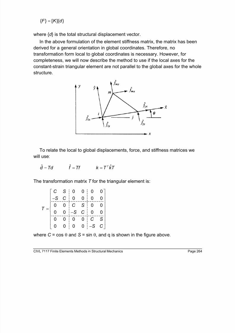
In the above formulation of the element stiffness matrix, the matrix has been
derived for a general orientation in global coordinates. Therefore, no
transformation form local to global coordinates is necessary. However, for
completeness, we will now describe the method to use if the local axes for the
constant-strain triangular element are not parallel to the global axes for the whole
structure.
To relate the local to global displacements, force, and stiffness matrices we
will use:
T k T k Tf f Td d T ˆˆˆ ===
The transformation matrix T for the triangular element is:
where C = cos θ and S = sin θ, and q is shown in the figure above.
0 0 0 0
0 0 0 0
0 0 0 0
0 0 0 0
0 0 0 0
0 0 0 0
C S
S C
C ST S C
C S
S C
−
= −
−
8/10/2019 Caso Placa 4
http://slidepdf.com/reader/full/caso-placa-4 22/42
CIVL 7117 Finite Elements Methods in Structural Mechanics Page 265
Step 6 - Solve for the Nodal Displacements
Step 7 - Solve for Element Forces and Stress
Having solved for the nodal displacements, we can obtain strains and
stresses in x and y directions in the elements by using:
[ ] [ ][ ] B d D B d ε σ = =
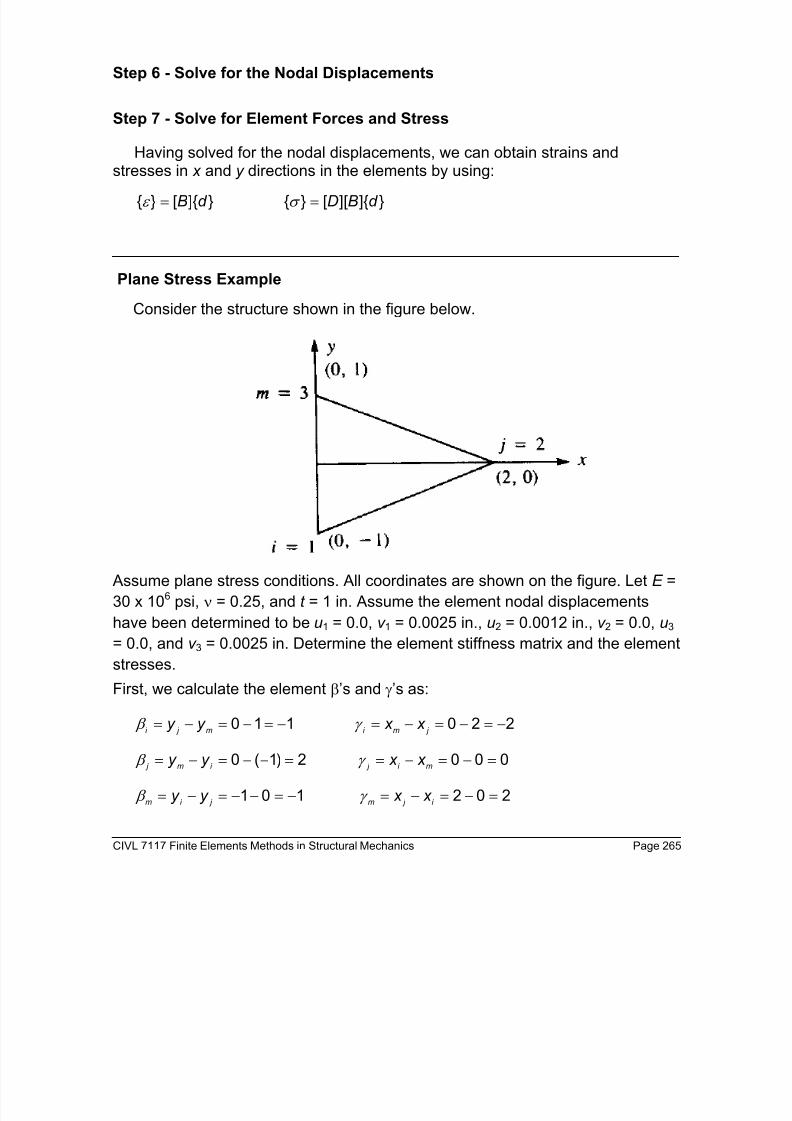
Plane Stress Example
Consider the structure shown in the figure below.
Assume plane stress conditions. All coordinates are shown on the figure. Let E =
30 x 106 psi, ν = 0.25, and t = 1 in. Assume the element nodal displacements
have been determined to be u1 = 0.0, v 1 = 0.0025 in., u2 = 0.0012 in., v 2 = 0.0, u3
= 0.0, and v 3 = 0.0025 in. Determine the element stiffness matrix and the element
stresses.
First, we calculate the element β’s and γ’s as:
220110 −=−=−=−=−=−= j mi m j i
x x y y γ β
0002)1(0 =−=−==−−=−=mi j i m j
x x y y γ β
202101 =−=−=−=−−=−=i j m j i m
x x y y γ β
8/10/2019 Caso Placa 4
http://slidepdf.com/reader/full/caso-placa-4 23/42
CIVL 7117 Finite Elements Methods in Structural Mechanics Page 266
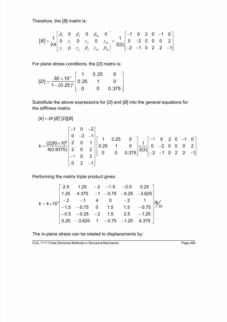
Therefore, the [B] matrix is:
[ ]
0 0 0 1 0 2 0 1 01 1
0 0 0 0 2 0 0 0 22 2(2)
2 1 0 2 2 1
i j m
i j m
i i j j m m
B A
β β β
γ γ γ
γ β γ β γ β
− − = = −
− − −
For plane stress conditions, the [D] matrix is:
−×
=
375.000
0125.0
025.01
)25.0(1
1030][
2
6
D
Substitute the above expressions for [D] and [B] into the general equations for
the stiffness matrix:
]][[][][ BDBtAk T =
6
1 0 2
0 2 11 0.25 0 1 0 2 0 1 0
2 0 1(2)30 10 1
0.25 1 0 0 2 0 0 0 24(0.9375) 2(2)2 0 20 0 0.375 2 1 0 2 2 1
1 0 2
0 2 1
k
− − − − − − ×
= − − − − −
−
Performing the matrix triple product gives:
inlbk
−−−
−−−−
−−−
−−−
−−−−
−−−
×=
375.425.175.01625.325.0
25.15.25.1225.05.0
75.05.15.1075.05.1
120412
625.325.075.01375.425.1
25.05.05.1225.15.2
104 6
The in-plane stress can be related to displacements by:

8/10/2019 Caso Placa 4
http://slidepdf.com/reader/full/caso-placa-4 24/42
CIVL 7117 Finite Elements Methods in Structural Mechanics Page 267
]][[ d BD=σ
6
0.0
0.00251 0.25 0 1 0 2 0 1 0
0.001230 10 1
0.25 1 0 0 2 0 0 0 20.9375 2(2) 0.00 0 0.375 2 1 0 2 2 1
0.0
0.0025
x
y
xy
in
in
in
σ
σ τ
− − ×
= − − − −
The stresses are:
−
=
psi
psi
psi
xy
y
x
000,15
800,4
200,19
τ
σ
σ
Recall, the relationships for principal stresses and principal angle in two-
dimensions are:
max
2
2
122
σ τ σ σ σ σ
σ =+
−+
+=
xy
y x y x
min
2
2
222
σ τ σ σ σ σ σ =+
−−+=
xy
y x y x
−= −
y x
xy
pσ σ
τ θ
2tan
2
1 1
Therefore:
( ) psi 639,28000,152
800,4200,19
2
800,4200,19 2
2
1 =−+
−+
+=σ
( ) psi 639,4000,152
800,4200,19
2
800,4200,19 2
2
1 −=−+
−−
+=σ
o
p3.32
800,4200,19
)000,15(2tan
2
1 1 −=
−
−= −θ

8/10/2019 Caso Placa 4
http://slidepdf.com/reader/full/caso-placa-4 25/42
CIVL 7117 Finite Elements Methods in Structural Mechanics Page 268
Treatment of Body and Surface Forces
The general force vector is defined as:
∫∫ ++=S
T
V
T dST N P dV X N f ][][
Body Force
Let’s consider the first term of the above equation.
[ ] = ∫ T
b
V
f N X dV
where
=
b
b
X X
Y
where X b and Y b are the weight densities in the x and y directions, respectively.
The force may reflect the effects of gravity, angular velocities, or dynamic inertial
forces.
The integration of the f b is simplified if the origin of the coordinate system is
chosen at the centroid of the element, as shown in the figure below. With the
origin placed at the centroid, we can use the definition of a centroid.
For a given thickness, t , the body force term becomes:
[ ] [ ] T T
b
V A
f N X dV t N X dA= =∫ ∫
0=∫ A
x dA
0=∫ A
y dA
8/10/2019 Caso Placa 4
http://slidepdf.com/reader/full/caso-placa-4 26/42
CIVL 7117 Finite Elements Methods in Structural Mechanics Page 269
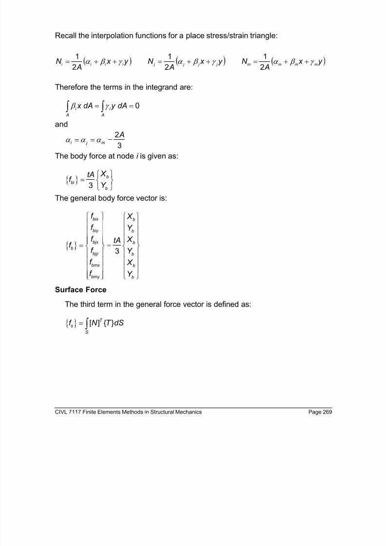
Recall the interpolation functions for a place stress/strain triangle:
( ) ( ) ( )y x A
N y x A
N y x A
N mmmm j j j j i i i i
γ β α γ β α γ β α ++=++=++=2
1
2
1
2
1
Therefore the terms in the integrand are:
0 β γ = =∫ ∫i i
A A
x dA y dA
and
2
3i j m
Aα α α = = =
The body force at node i is given as:
3
=
b
bi
b
X tAf
Y
The general body force vector is:
3
bix b
biy b
bjx b
b
bjy b
bmx b
bmy b
f X
f Y
f X tAf
f Y f X
f Y
= =
Surface Force
The third term in the general force vector is defined as:
[ ] = ∫ T
s
S
f N T dS
8/10/2019 Caso Placa 4
http://slidepdf.com/reader/full/caso-placa-4 27/42
CIVL 7117 Finite Elements Methods in Structural Mechanics Page 270
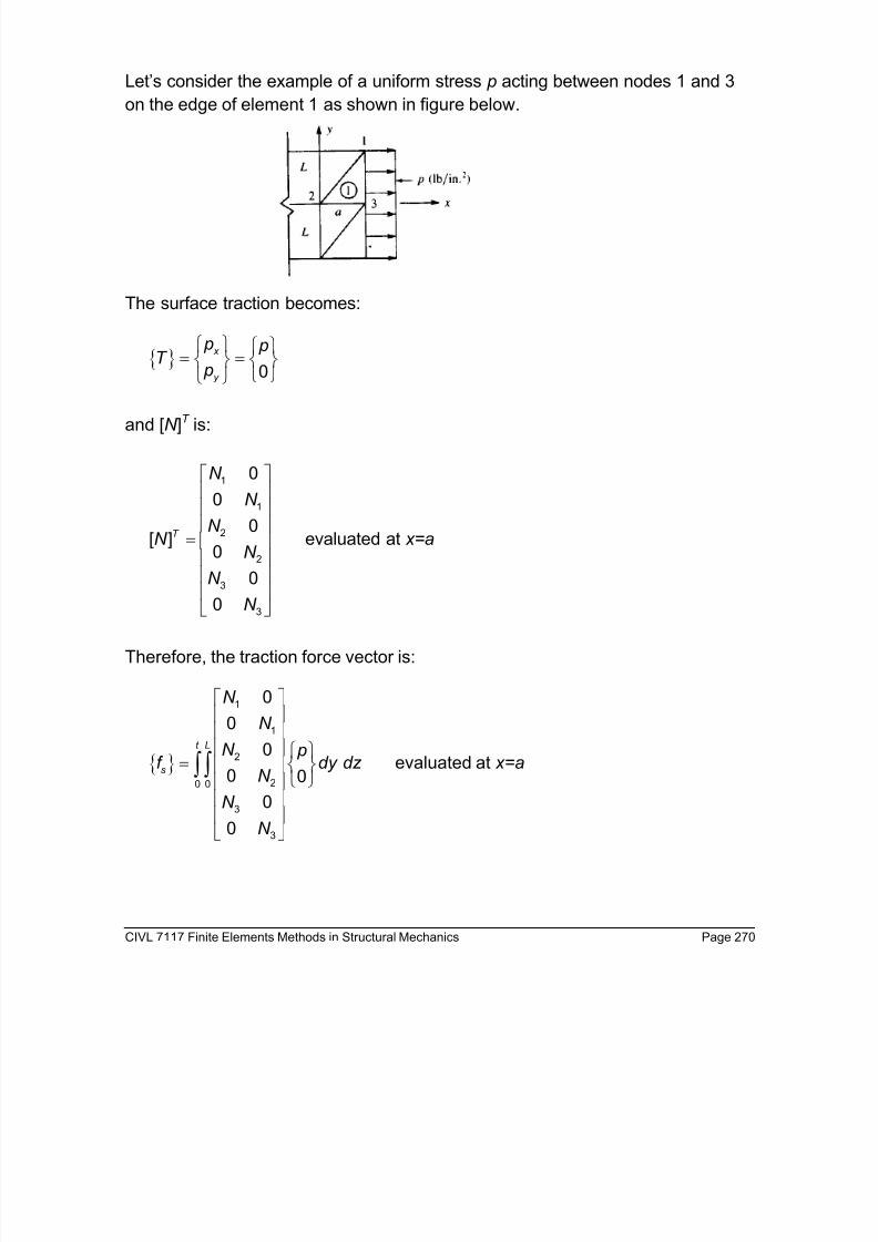
Let’s consider the example of a uniform stress p acting between nodes 1 and 3
on the edge of element 1 as shown in figure below.
The surface traction becomes:
0
= =
x
y
p pT
p
and [N ]T is:
1
1
2
2
3
3
0
0
0[ ]
0
0
0
=
T
N
N
N N
N
N
N
evaluated at x=a
Therefore, the traction force vector is:
1
1
2
20 0
3
3
0
0
0
0 0
0
0
=
∫ ∫
t L
s
N
N
N pf dy dz N
N
N
evaluated at x=a

8/10/2019 Caso Placa 4
http://slidepdf.com/reader/full/caso-placa-4 28/42
CIVL 7117 Finite Elements Methods in Structural Mechanics Page 271
After some simplification, the traction force vector is:
1
2
0
3
0
0
0
=
∫
L
s
N p
N p
f t dy
N p
The interpolation function for i = 1 is:
( )1
2α β γ = + +i i i i N x y
A
For convenience, let’s choose the coordinate system shown in the figure below.
Recall:
α = −i j m j m x y y x
with i = 1, j = 2, and m = 3, we get
1 2 3 2 3α = − x y y x
If we substitute the coordinates of the triangle show above in the above equation
we get:

8/10/2019 Caso Placa 4
http://slidepdf.com/reader/full/caso-placa-4 29/42
CIVL 7117 Finite Elements Methods in Structural Mechanics Page 272
1 0α =
Similarly, we can find:
1 10 β γ = = a
Therefore, the interpolation function, N 1 is:
12
=ay
N A
The remaining interpolation function, N 2 and N 2 are:
2 3
( )
2 2
− −= =
L a x Lx ay N N
A A
Substituting the interpolation function in the traction force vector expression
gives:
1
1
2
2
3
3
1
0
0
2 0
10
= =
s x
s y
s x
s
s y
s x
s y
f
f
f pLt f
f
f f
Explicit Expression for the Constant-Strain Triangle Stiffness Matrix
Usually the stiffness matrix is computed internally by computer programs, but
since we are not computers, we need to explicitly evaluate the stiffness matrix.
For a constant-strain triangular element, considering the plane strain case, recall
that:
[ ] [ ] [ ][ ]= T k tA B D B
where [D] for plane strain is:

8/10/2019 Caso Placa 4
http://slidepdf.com/reader/full/caso-placa-4 30/42
CIVL 7117 Finite Elements Methods in Structural Mechanics Page 273
( )( )
−
−
−
−+=
ν
ν ν
ν ν
ν ν 5.000
01
01
211][
E D
Substituting the appropriate definition into the above triple product gives:
0
01 0
0[ ] 1 0
04 (1 )(1 2 )0 0 0.5
0
0
β γ
γ β ν ν
β γ ν ν
γ β ν ν ν
β γ
γ β
− = − + − −
i i
i i
j j
j j
m m
m m
tE k
A
0 0 0
0 0 0
β β β
γ γ γ
γ β γ β γ β
×
i j m
i j m
i i j j m m
Therefore the global stiffness matrix is:
8/10/2019 Caso Placa 4
http://slidepdf.com/reader/full/caso-placa-4 31/42
CIVL 7117 Finite Elements Methods in Structural Mechanics Page 274
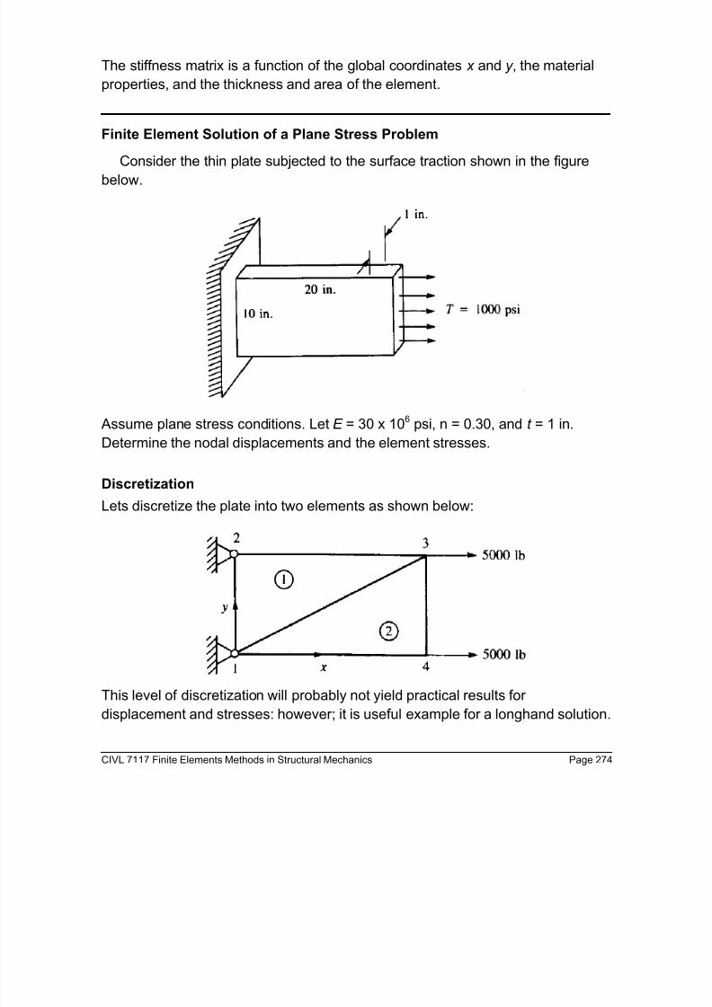
The stiffness matrix is a function of the global coordinates x and y , the material
properties, and the thickness and area of the element.
Finite Element Solution of a Plane Stress Problem
Consider the thin plate subjected to the surface traction shown in the figure
below.
Assume plane stress conditions. Let E = 30 x 106 psi, n = 0.30, and t = 1 in.
Determine the nodal displacements and the element stresses.
Discretization
Lets discretize the plate into two elements as shown below:
This level of discretization will probably not yield practical results for
displacement and stresses: however; it is useful example for a longhand solution.
8/10/2019 Caso Placa 4
http://slidepdf.com/reader/full/caso-placa-4 32/42
CIVL 7117 Finite Elements Methods in Structural Mechanics Page 275
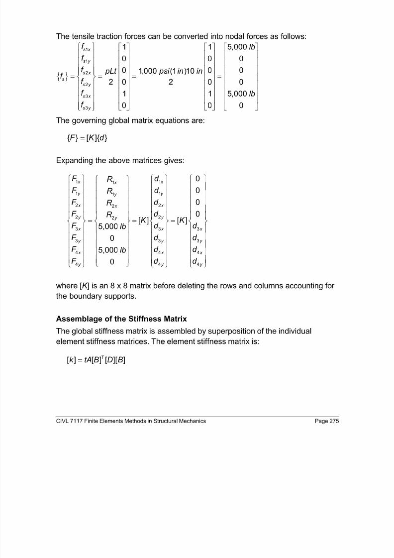
The tensile traction forces can be converted into nodal forces as follows:
1
1
2
2
3
3
1 1 5,000
0 0 0
0 0 01,000 (1 )10
2 20 0 01 1 5,000
0 0 0
s x
s y
s x
s
s y
s x
s y
f lb
f
f pLt psi in inf
f
f lb
f
= = = =
The governing global matrix equations are:
[ ] =F K d
Expanding the above matrices gives:
1 11
1 11
2 22
2 22
3 3 3
3 3 3
4 4 4
4 4 4
0
0
0
0[ ] [ ]
5,000
0
5,000
0
= = =
x x x
y y y
x x x
y y y
x x x
y y y
x x x
y y y
F d R
F d R
F d R
F d R K K
F d d lb
F d d
F d d lb
F d d
where [K ] is an 8 x 8 matrix before deleting the rows and columns accounting for
the boundary supports.
Assemblage of the Stiffness Matrix
The global stiffness matrix is assembled by superposition of the individual
element stiffness matrices. The element stiffness matrix is:
[ ] [ ] [ ][ ]= T k tA B D B

8/10/2019 Caso Placa 4
http://slidepdf.com/reader/full/caso-placa-4 33/42
CIVL 7117 Finite Elements Methods in Structural Mechanics Page 276
For element 1: the coordinates are x i = 0, y i = 0, x j = 20, y j = 10, x m = 0, and y m =
10. The area of the triangle is:
The matrix [B] is:
0 0 01
[ ] 0 0 02
β β β
γ γ γ γ β γ β γ β
=
i j m
i j m
i i j j m m
B A
We need to calculate the element β’s and γ’s as:
10 10 0 0 20 20 β γ = − = − = = − = − = −i j m i m j y y x x
1 10 0 10 0 0 0 β γ = − = − = = − = − = j m j i my y x x
0 10 10 20 0 20 β γ = − = − = − = − = − =m i j m i j y y x x
Therefore, the [B] matrix is:
0 0 10 0 10 01 1[ ] 0 20 0 0 0 20
20020 0 0 10 20 10
− = − − −
Bin
For plane stress conditions, the [D] matrix is:
61 0.3 0
30 10[ ] 0.3 1 0
0.910 0 0.35
× =
D psi
2=
bh
A
2(20)(10)100 .
2= = A in

8/10/2019 Caso Placa 4
http://slidepdf.com/reader/full/caso-placa-4 34/42
CIVL 7117 Finite Elements Methods in Structural Mechanics Page 277
Therefore:
6
0 0 20
0 20 01 0.3 0
10 0 030(10 )
[ ] [ ] 0.3 1 0200(0.91) 0 0 100 0 0.35
10 0 20
0 20 10
− −
= −
−
T
B D
Simplifying the above expression gives:
6
0 0 7
6 20 0
10 3 030(10 )[ ] [ ]200(0.91) 0 0 3.5
10 3 7
6 20 3.5
T B D
− − −
= − −
−
The element stiffness matrix is:
[ ] [ ] [ ][ ]= T k tA B D B
therefore:
6
0 0 7
6 20 0
10 3 0(0.15)(10 )[ ] [ ][ ] 1(100)
0.91 0 0 3.5
10 3 7
6 20 3.5
T tA B D B
− − −
= − −
−
0 0 10 0 10 01
0 20 0 0 0 20200
20 0 0 10 20 10
− × − − −

8/10/2019 Caso Placa 4
http://slidepdf.com/reader/full/caso-placa-4 35/42
CIVL 7117 Finite Elements Methods in Structural Mechanics Page 278
Simplifying the above expression gives:
1 1 3 3 2 2
140 0 0 70 140 70
0 400 60 0 60 400
0 60 100 0 100 6075,000[ ]
0.91 70 0 0 35 70 35
140 60 100 70 240 130
70 400 60 35 130 435
u v u v u v
k
− − − − −
− −=
− − − − −
− − −
For element 2: the coordinates are x i = 0, y i = 0, x j = 20, y j = 0, x m = 20, and y m =
10. The area of the triangle is:
We need to calculate the element β’s and γ’s as:
0 10 10 20 20 0 β γ = − = − = − = − = − =i j m i m j y y x x
1 10 0 10 0 20 20 β γ = − = − = = − = − = − j m j i my y x x
0 0 0 20 0 20 β γ = − = − = = − = − =m i j m i j y y x x
Therefore, the [B] matrix is:
10 0 10 0 0 01 1[ ] 0 0 0 20 0 20
2000 10 20 10 20 0
− = − − −
Bin
2(20)(10)100 .
2= = A in

8/10/2019 Caso Placa 4
http://slidepdf.com/reader/full/caso-placa-4 36/42
CIVL 7117 Finite Elements Methods in Structural Mechanics Page 279
For plane stress conditions, the [D] matrix is:
61 0.3 0
30 10[ ] 0.3 1 0
0.910 0 0.35
× =
D psi
Therefore:
6
10 0 0
0 0 101 0.3 0
10 0 2030(10 )[ ] [ ] 0.3 1 0
200(0.91) 0 20 100 0 0.35
0 0 20
0 20 0
− − − = −
T B D
Simplifying the above expression gives:
6
10 3 0
0 0 3.5
10 3 730(10 )[ ] [ ]
200(0.91) 0 20 3.5
6 0 7
6 20 0
− − − −
= −
−
T B D
The element stiffness matrix is:
[ ] [ ] [ ][ ]= T k tA B D B
therefore:
6
10 3 0
0 0 3.510 3 7(0.15)(10 )
[ ] [ ][ ] 1(100)0.91 0 20 3.5
6 0 7
6 20 0
− −
− −
= −
−
T tA B D B
8/10/2019 Caso Placa 4
http://slidepdf.com/reader/full/caso-placa-4 37/42
CIVL 7117 Finite Elements Methods in Structural Mechanics Page 280
10 0 10 0 0 01
0 0 0 20 0 20200
0 10 20 10 20 0
− × − − −
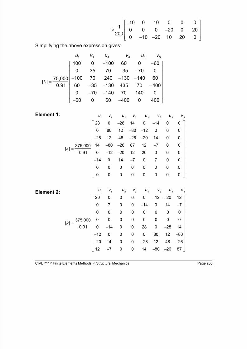
Simplifying the above expression gives:
1 1 4 4 3 3
100 0 100 60 0 60
0 35 70 35 70 0
100 70 240 130 140 6075,000[ ]
0.91 60 35 130 435 70 400
0 70 140 70 140 0
60 0 60 400 0 400
u v u v u v
k
− − − − − − −
= − − −
− −
− −
Element 1:
Element 2:
1 1 2 2 3 3 4 4
28 0 28 14 0 14 0 0
0 80 12 80 12 0 0 0
28 12 48 26 20 14 0 0
14 80 26 87 12 7 0 0375,000[ ]
0.91 0 12 20 12 20 0 0 0
14 0 14 7 0 7 0 00 0 0 0 0 0 0 0
0 0 0 0 0 0 0 0
− −
− −
− − −
− − −=
− −
− −
u v u v u v u v
k
1 1 2 2 3 3 4 4
20 0 0 0 0 12 20 12
0 7 0 0 14 0 14 7
0 0 0 0 0 0 0 00 0 0 0 0 0 0 0375,000
[ ]0.91 0 14 0 0 28 0 28 14
12 0 0 0 0 80 12 80
20 14 0 0 28 12 48 26
12 7 0 0 14 80 26 87
− −
− −
=− −
− −
− − −
− − −
u v u v u v u v
k

8/10/2019 Caso Placa 4
http://slidepdf.com/reader/full/caso-placa-4 38/42
CIVL 7117 Finite Elements Methods in Structural Mechanics Page 281
Using the superposition, the total global stiffness matrix is:
1 1 2 2 3 3 4 4
48 0 28 14 0 26 20 12
0 87 12 80 26 0 14 7
28 12 48 26 20 14 0 0
14 80 26 87 12 7 0 0375,000[ ]
0.91 0 26 20 12 48 0 28 14
26 0 14 7 0 87 12 80
20 14 0 0 28 12 48 26
12 7 0 0 14 80 26 87
− − −
− − −
− − −
− −=
− − −
− − −
− − −
− − −
u v u v u v u v
k
The governing global matrix equations are:
[ ] =F K d
1
1
2
2
48 0 28 14 0 26 20 12
0 87 12 80 26 0 14 7
28 12 48 26 20 14 0 0
14 80 26 87 12 7 0 0
0 26 20 12 48 0 28 1426 0 14 7 0 87 12 80
20 14 0 0 28 12 48 26
12 7 0 0 14 80 26 87
375,000
0.915,0000
500
0
− − −
− − −
− − −
− −
− − −− − −
− − −
− − −
=
x
y
x
y
R
R
R
R
lb
lb
1
1
2
2
3
3
4
4
x
y
x
y
x
y
x
y
d
d
d
d
d d
d
d
Applying the boundary conditions:
1 1 2 20= = = = x y x y
d d d d
The governing equations are:
3
3
4
4
5,000 48 0 28 14
0 0 87 12 80375,000
0.915,000 28 12 48 26
0 14 80 26 87
x
y
x
y
d lb
d
d lb
d
− − = − −
− −
8/10/2019 Caso Placa 4
http://slidepdf.com/reader/full/caso-placa-4 39/42
CIVL 7117 Finite Elements Methods in Structural Mechanics Page 282
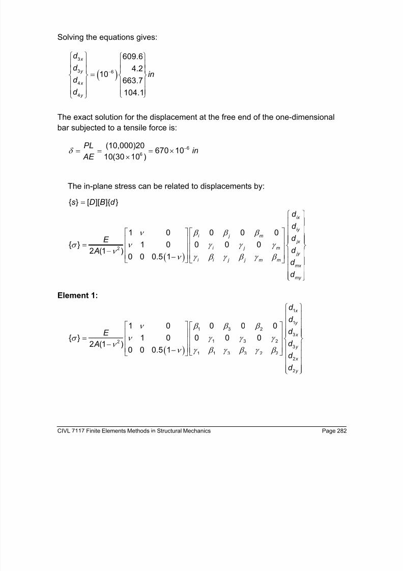
Solving the equations gives:
( )
3
3 6
4
4
609.6
4.210
663.7
104.1
−
=
x
y
x
y
d
d in
d
d
The exact solution for the displacement at the free end of the one-dimensional
bar subjected to a tensile force is:
6
6
(10,000)20670 10
10(30 10 )δ
−= = = ××
PLin
AE
The in-plane stress can be related to displacements by:
[ ][ ] =s D B d
( )2
1 0 0 0 0
1 0 0 0 02 (1 )
0 0 0.5 1
ν β β β
σ ν γ γ γ ν
ν γ β γ β γ β
= − −
ix
iy
i j m
jx
i j m
jy
i i j j m m
mx
my
d
d
d E
d A
d d
Element 1:
( )
1
1
1 3 2
3
1 3 223
1 1 3 3 2 2
2
2
1 0 0 0 0
1 0 0 0 02 (1 )
0 0 0.5 1
ν β β β
σ ν γ γ γ ν
ν γ β γ β γ β
= −
−
x
y
x
y
x
y
d
d
d E
d A
d
d
8/10/2019 Caso Placa 4
http://slidepdf.com/reader/full/caso-placa-4 40/42
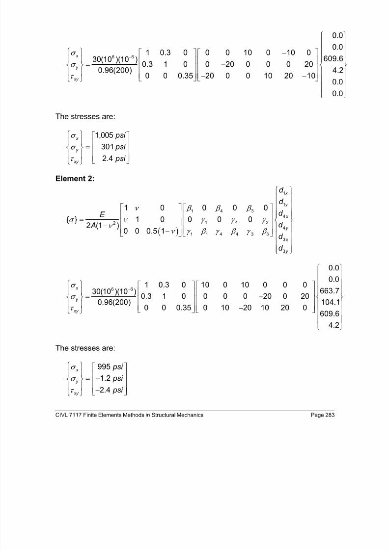
CIVL 7117 Finite Elements Methods in Structural Mechanics Page 283
6 6
0.0
0.01 0.3 0 0 0 10 0 10 0
609.630(10 )(10 )0.3 1 0 0 20 0 0 0 20
0.96(200) 4.20 0 0.35 20 0 0 10 20 10
0.00.0
σ
σ
τ
−
− = −
− −
x
y
xy
The stresses are:
1,005
301
2.4
σ
σ
τ
=
x
y
xy
psi
psi
psi
Element 2:
( )
1
1
1 4 3
4
1 4 324
1 1 4 4 3 3
3
3
1 0 0 0 0
1 0 0 0 02 (1 )
0 0 0.5 1
ν β β β
σ ν γ γ γ ν
ν γ β γ β γ β
= − −
x
y
x
y
x
y
d
d
d E
d A
d
d
6 6
0.0
0.01 0.3 0 10 0 10 0 0 0
663.730(10 )(10 )0.3 1 0 0 0 0 20 0 20
0.96(200) 104.10 0 0.35 0 10 20 10 20 0
609.6
4.2
σ
σ
τ
−
= −
−
x
y
xy
The stresses are:
995
1.2
2.4
σ
σ
τ
= − −
x
y
xy
psi
psi
psi
8/10/2019 Caso Placa 4
http://slidepdf.com/reader/full/caso-placa-4 41/42
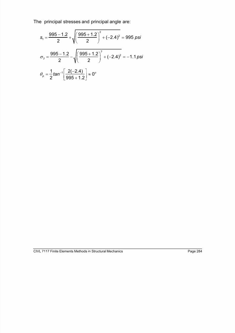
CIVL 7117 Finite Elements Methods in Structural Mechanics Page 284
The principal stresses and principal angle are:
2
2
1
995 1.2 995 1.2( 2.4) 995
2 2
− + = + + − =
s psi
22
2
995 1.2 995 1.2( 2.4) 1.1
2 2σ
− + = − + − = −
psi
11 2( 2.4)0
2 995 1.2θ − − = ≈ +
o
p tan

8/10/2019 Caso Placa 4
http://slidepdf.com/reader/full/caso-placa-4 42/42
Problems
16. Do problems 6.5, 6.6, 6.9, 6.10, and 6.13 on pages 301 - 306 in yourtextbook “A First Course in the Finite Element Method” by D. Logan.
17. Rework the plane stress problem given on page 291 in your textbook “A
First Course in the Finite Element Method” by D. Logan using SAP2000 to
do analysis. Start with the simple two element model. Continuously refine
your discretization by a factor of two each time until your FEM solution is in
agreement with the exact solution for both displacements and stress. Howmany elements did you need?