carlos a. perez eman m. el-sheikh* clark glymour€¦ · · 2011-08-1888 c.a. perez et al....

86 Int. J. Computers in Healthcare, Vol. 1, No. 1, 2010

Copyright © 2010 Inderscience Enterprises Ltd.

Discovering effective connectivity among brain regions from functional MRI data

Carlos A. Perez Institute for Human and Machine Cognition, 15 SE Osceola Avenue, Ocala, FL 34471, USA E-mail: [email protected]

Eman M. El-Sheikh* College of Arts and Sciences, University of West Florida, 11000 University Parkway, Pensacola, FL 32514, USA E-mail: [email protected] *Corresponding author

Clark Glymour Department of Philosophy, Baker Hall 135L, Carnegie Mellon University, Pittsburgh, PA 15213 USA E-mail: [email protected]

Abstract: Functional magnetic resonance imaging (fMRI) data have been used for identifying brain regions that activate when a subject is presented a stimulus or performs a task. Beyond identifying which regions of the brain are active during a task, it is also of interest to discover causal relationships among activity in those regions, that is, which regions of the brain influence, which other regions of the brain during a task. Two algorithms for causal discovery were applied to fMRI data, the greedy equivalence search (GES) algorithm and the independent multiple-sample greedy equivalence search (iMAGES). GES applies to individual datasets, and iMAGES to multiple datasets. We consider the stability of the GES results across subjects and experimental repetitions with the same subject. We find that some iMAGES connections agree with previous knowledge of the functional roles of the brain regions. The strengths and limitations of the research work and opportunities for future work are also discussed.

Keywords: artificial intelligence; brain regions; causal modelling; effective connectivity; functional magnetic resonance imaging; fMRI; healthcare; local search; knowledge discovery.

Reference to this paper should be made as follows: Perez, C.A., El-Sheikh, E.M. and Glymour, C. (2010) ‘Discovering effective connectivity among brain regions from functional MRI data’, Int. J. Computers in Healthcare, Vol. 1, No. 1, pp.86–102.

Discovering effective connectivity among brain regions 87

Biographical notes: Carlos A. Perez is a Research Associate at the Florida Institute for Human and Machine Cognition. He received his BSc (2004) in Computer Science from EAFIT University in Colombia. He received his MSc (2009) in Computer Science at the University of West Florida. His research interests include machine learning and data mining.

Eman M. El-Sheikh is the Associate Dean for the College of Arts and Sciences and an Associate Professor of Computer Science at the University of West Florida. She received her PhD (2002) and MSc (1995) in Computer Science from Michigan State University and BSc (1992) in Computer Science from the American University in Cairo. Her research interests include artificial intelligence-based techniques and tools for education, including the development of intelligent tutoring systems and adaptive learning tools, agent-based architectures, knowledge-based systems, and computer science education.

Clark Glymour is an Alumni University Professor at Carnegie Mellon University, Senior Research Scientist at the Florida Institute of Human and Machine Cognition, and Adjunct Professor of History and Philosophy of Science at the University of Pittsburgh. He has been a Guggenheim Fellow, a Fellow of the Center for Advanced Study in the Behavioral Sciences, and a Phi Beta Kappa Lecturer. His collaborative work with Peter Spirtes and Richard Scheines, Causation, Prediction and Search (Springer Lecture Notes in Statistics, 1993) introduced the first feasible, consistent algorithms for search and prediction with graphical causal models.

1 Introduction

Functional magnetic resonance imaging (fMRI) measures changes in the blood oxygenation levels (BOLD) related to neural activity in the brain in response to a presented stimulus (Clare, 1997). The fMRI BOLD signal produces a 3D multivariate time series with signals localised in small regions – voxels. Statistical thresholds compared to a rest state determine which voxels show significant activation; those voxels are clustered into regions of interest (ROI). Beyond identifying which regions of the brain are active during a task, it is also of interest to discover causal relationships among activity in those regions. In fMRI terminology, the causal relationship between two brain regions is known as effective connectivity, characterised as “the influence one neural system exerts over another” (Friston, 1994).

Analysing fMRI data to discover effective brain connectivity presents a number of difficulties (Ramsey et al., 2010). The fMRI BOLD signal is an indirect measurement of neural activity, and it measures a delayed effect that might vary among subjects, among trials, or even among brain regions of the same subject. FMRI data from multiple subjects cannot be straightforwardly combined without destroying statistical information, so analysis of such data requires the use of search methods that avoid combining the data. Additionally, different subjects might have different but overlapping sets of ROIs and the signal strengths from the same brain regions may differ from subject to subject.

The present work applies and evaluates two algorithms for causal discovery on fMRI data. These algorithms are the greedy equivalence search (GES) algorithm (Meek, 1997) and the independent multiple-sample greedy equivalence search (iMAGES) algorithm

88 C.A. Perez et al.

(Ramsey et al., 2010), which is a generalisation of the GES algorithm for handling multiple datasets. These algorithms have previously been applied to a different set of fMRI data from a different experimental task and extensively tested on simulated data (Ramsey et al., 2010). The result of running the algorithms on the fMRI data is analysed for stability across subjects and across experimental repetitions. To evaluate the validity of the resulting causal structures discovered by the algorithms, the results are assessed using previous knowledge about the functional roles of the involved ROIs.

Section 2 provides a brief overview of approaches for discovering effective connectivity from fMRI data. Section 3 describes the data to be analysed and the experimental setup. Section 4 presents the GES and iMAGES algorithms and Section 5 presents the results obtained after applying these algorithms to the data, and provides an analysis of the results in regards to stability and validity of the resulting structures. Finally, Section 6 presents the research conclusions and opportunities for future work.

2 Related work

Effective brain connectivity has been studied using various techniques, including some specifically-tailored methods and other more general techniques. Structural equation models (SEMs) represent the causal relationships as a set of linear equations. There is one equation for each variable that is an effect. Each function represents the effect variable as a linear function of the parents or causes in the model, multiplied by a coefficient that represents the strength of the relationship. Each equation also contains a term for random disturbances in the model. Usually, SEMs are used as a confirmatory tool for a hypothesised causal model, or to assess the strength of the relationships in different experimental setups (e.g., Walsh et al., 2008; Tsubomi et al., 2009; Tourville et al., 2008). But some studies have tried to use SEMs as an exploratory tool (e.g., Laird et al., 2008; Zhuang et al., 2008).

Granger (1969) causality is used to determine if a time series in one variable forecasts a time series in other variables. Granger causality is performed through a series of tests on lagged values of the time series; in the case of fMRI data, the time series are usually averages of BOLD signals within a ROI (e.g., Deshpande et al., 2008). Other studies have used modifications of Granger causality for the same purpose (e.g., Dhamala et al., 2008). One limitation of Granger causality is that it cannot determine whether a causal relationship is direct or mediated.

Dynamic causal modelling (DCM) is a technique that originated from the neuroimaging community (Friston et al., 2003). DCM is proposed as a confirmatory rather than as an exploratory technique for causal modelling of effective connectivity. DCM models the effective connectivity in the brain as a non-linear and dynamic process. A probability distribution over the parameter values of a DCM model is estimated by expectation maximisation. In a DCM model, the inputs are deterministic and are explicit from the experimental setup; these inputs influence ROIs, which in turn may influence other ROIs producing a measured output that corresponds to the observed BOLD signal. Examples of studies using DCM for studying effective connectivity are Kasess et al. (2008), Acs and Greenlee (2008), Grefkes et al. (2008), Schlösser et al. (2008) and Chen et al. (2009). Some studies have already started to propose some modifications to the basic DCM approach (e.g., Marreiroset al., 2008; Stephan et al., 2008), and Bayesian


model selection has recently been proposed to explore for DCM models (Stephan et al., 2009).

Another technique that has been used as a data-driven exploratory tool for effective connectivity is partial correlation analysis (Fransson and Marrelec, 2008). Partial correlation analysis is a data-driven approach that computes the conditional correlation between any pair of ROIs with respect to the remaining ROI. Partial correlation analysis does not allow determination of the directionality of the causal relationships, and can, and typically will, introduce spurious connections.

Dynamic Bayesian networks are specialisations of Bayesian networks that model temporal processes. Kim et al. (2008) have used the representation for fMRI data. Like Granger causality models, dynamic Bayesian networks represent the time ordering of the events, but the search procedures for static Bayesian networks are used.

Stimulus-locked vector autoregressive models (SloVAR) are exploratory tools specifically tailored to find directed dynamic relationships among multiple brain regions in a special type of fMRI experimental setup known as slow event-related fMRI (Thompson and Siegle, 2009). In a slow event-related fMRI experimental setup, the stimulus is presented briefly and separated by an intertrial interval from ten to 20 seconds allowing the hemodynamic response to fully occur and decay. SloVAR is an adaptation of vector autoregressive models (VAR), where the connectivity coefficients vary as a function of lag and time relative to the last stimulus onset. The output of SloVAR modelling is a set of surfaces representing the directed relationships of each structure in the model at each lag to each other structure. SloVAR models have the same limitation as Granger causality: they cannot determine whether a causal relationship is direct or mediated.

3 Data and experimental setup

The fMRI data that will be analysed are from Tom et al. (2007), who used an event-related design in which subjects were presented an event or stimulus and fMRI recordings of the BOLD response were taken at regular intervals. The participants of the experiment were asked to decide whether to accept or reject mixed gambles that offered a 50/50 chance of either gaining one amount of money or losing another amount.

The objective of the experiment was to investigate which brain system represents the potential losses versus gains when the decision is being made. To convince the participants that the experiment consisted of real gambling, they were asked to bring $60 in cash, and they were told that this was the maximum amount that they could possibly lose. But, due to an initial endowment of $30 in cash given to all the participants, they all left with a net gain. The initial $30 was given during the pre-testing sessions at least a week before the experiment, in order to minimise the potential risk seeking in response to this unexpected income.

The experiment included 16 participants. They were presented with three runs of 85 to 86 trials. During each trial, the participants were presented with a display showing the size of the potential gain and the potential loss for three seconds. The potential gains ranged from $10 to $40 in $2 increments, and the potential losses ranged from $5 to $20 in $1 increments. The participants were asked to respond whether or not they would like to play each of the gambles presented. After each trial, a resting interval was presented.


To discourage the participants from using a fixed gambling strategy, they were asked to select as quickly as possible one of four responses on a four-button response box. The possible responses were: strongly accept, weakly accept, weakly reject and strongly reject. The participants were also told that, for each of the three runs, one trial would be selected at random from the trials for which they had accepted the gamble, and those three trials would be honoured with real money. But the gambles were not resolved during the scanning because the objective of the experiment was to investigate the brain mechanisms that represent the potential losses versus gains when the decision is being made, and not the actual experience of gaining or losing money. So, the selected gambles were resolved by a coin toss at the end of the session.

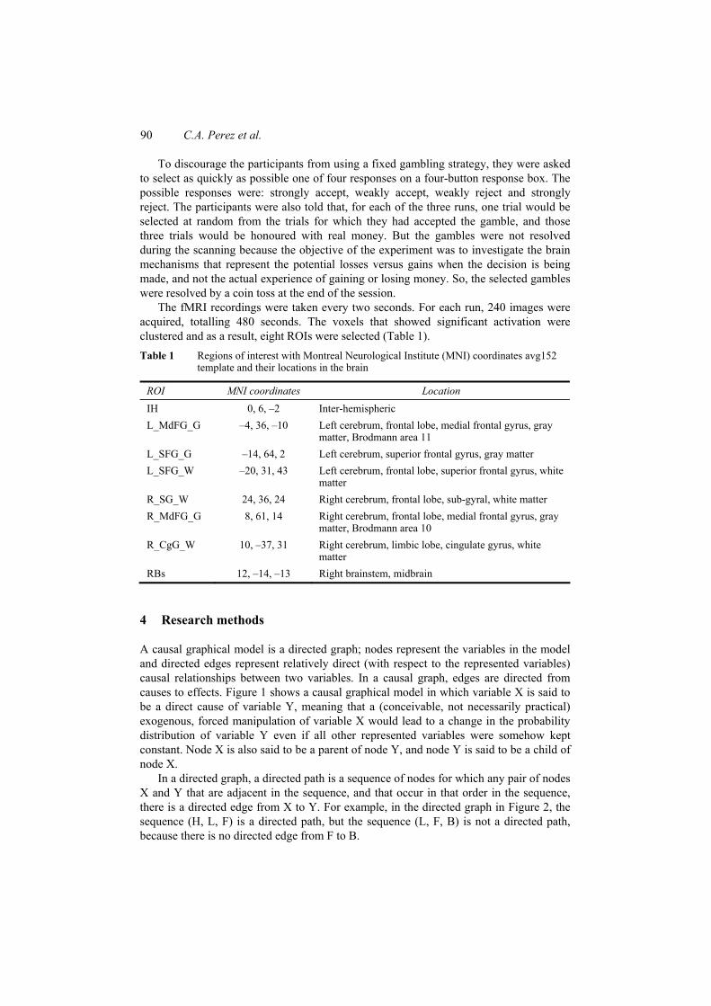
The fMRI recordings were taken every two seconds. For each run, 240 images were acquired, totalling 480 seconds. The voxels that showed significant activation were clustered and as a result, eight ROIs were selected (Table 1). Table 1 Regions of interest with Montreal Neurological Institute (MNI) coordinates avg152

template and their locations in the brain

ROI MNI coordinates Location IH 0, 6, –2 Inter-hemispheric L_MdFG_G –4, 36, –10 Left cerebrum, frontal lobe, medial frontal gyrus, gray

matter, Brodmann area 11 L_SFG_G –14, 64, 2 Left cerebrum, superior frontal gyrus, gray matter L_SFG_W –20, 31, 43 Left cerebrum, frontal lobe, superior frontal gyrus, white

matter R_SG_W 24, 36, 24 Right cerebrum, frontal lobe, sub-gyral, white matter R_MdFG_G 8, 61, 14 Right cerebrum, frontal lobe, medial frontal gyrus, gray

matter, Brodmann area 10 R_CgG_W 10, –37, 31 Right cerebrum, limbic lobe, cingulate gyrus, white

matter RBs 12, –14, –13 Right brainstem, midbrain

4 Research methods

A causal graphical model is a directed graph; nodes represent the variables in the model and directed edges represent relatively direct (with respect to the represented variables) causal relationships between two variables. In a causal graph, edges are directed from causes to effects. Figure 1 shows a causal graphical model in which variable X is said to be a direct cause of variable Y, meaning that a (conceivable, not necessarily practical) exogenous, forced manipulation of variable X would lead to a change in the probability distribution of variable Y even if all other represented variables were somehow kept constant. Node X is also said to be a parent of node Y, and node Y is said to be a child of node X.

In a directed graph, a directed path is a sequence of nodes for which any pair of nodes X and Y that are adjacent in the sequence, and that occur in that order in the sequence, there is a directed edge from X to Y. For example, in the directed graph in Figure 2, the sequence (H, L, F) is a directed path, but the sequence (L, F, B) is not a directed path, because there is no directed edge from F to B.


Figure 1 Example causal graphical model

Figure 2 Example causal graphical model

Causal graphs are acyclic. A directed acyclic graph (DAG) is a directed graph for which any directed path does not contain a node more than once. The directed graph in Figure 4 is also acyclic. In a DAG, a node X is said to be an ancestor of node Y if there is a directed path from X to Y. Also, a node Y is said to be a descendant of node X if there is a directed path from X to Y. In the DAG shown in Figure 2, node H is an ancestor of nodes B, L, F and C. Node F is a descendant of nodes H, B and L.

A causal graph is said to hold the Markov condition if, for any probability distribution for the causal model, the probability of any node in the graph is independent of its non-descendant nodes given its set of parent nodes (Pearl, 1988). For example, in the graph from Figure 2, the Markov condition entails the following independence, among others: B is independent of L given H.

The Markov condition allows the definition of an equivalence relationship between causal graphs known as the Markov equivalence (Spirtes et al., 1993). Two graphs are said to be Markov equivalent if they contain the same set of nodes and if the conditional independence relationships entailed by the Markov condition are the same in both graphs. Where a Markov equivalence class contains two graphs, one with a direction, X –> Y, and the other with a direction, X <– Y, the representation of the Markov equivalence class puts an undirected edge, X – Y, between the variables.


4.1 GES

The GES algorithm searches over the space of Markov equivalence classes using a scoring function to score a representative of each Markov equivalence class. The GES algorithm has two phases. The first phase starts with a Markov equivalence class containing no edges. Then it scores a representative of each Markov equivalence class resulting from adding one edge to the current Markov equivalence class. The Markov equivalence class that has the highest score is chosen. This first phase continues until there is no Markov equivalence class with an additional edge that increases the score.

The second phase is analogous to the first phase, except that the algorithm scores a representative of each Markov equivalence class resulting from removing one edge from the current Markov equivalence class. This phase is repeated until there is no Markov equivalence class with a removed edge that increases the score.

The GES scoring function is the Bayesian information criterion (BIC) given by (Schwarz, 1978):

2 ln( ) ln( ),= − +BIC ML k n

where ML is the maximum likelihood estimate of the model’s free parameters, k is the dimension of the model, and n is the sample size.

If certain assumptions are met, the posterior probability of the model given the data is a monotonic function of BIC. Under those and other assumptions – which are not entirely satisfied in fMRI modelling – the limit of the probability of finding the Markov equivalence class of the true model is provably equal to one, as the size of the dataset approaches infinity.

Adding a multiplicative constant c > 1 to the second term of the BIC function can help reduce false positive edges in the resulting graph without affecting the asymptotic properties of BIC. The BIC score with the penalty term c is:

2 ln( ) ln( ).BICc ML ck n= − +

4.2 iMAGES

The iMAGES algorithm is a generalisation of the GES algorithm (Ramsey et al., 2010). This generalisation assumes that there is a common causal structure that is responsible for generating the multiple datasets for all subjects. The iMAGES algorithm follows the GES procedure but, as its score function, it uses the average BIC score for the representative of each Markov equivalence class in several datasets. The score function for iMAGES is:

1

2 ,=

= − ∑m

ii

iMscore BICm

where m is the number of datasets, and BICi is the BIC score of the representative graph of the Markov equivalence class being evaluated using dataset i. iMAGES, thus, uses the data from multiple independent time series without merging the several datasets into a single dataset. Given the assumption that there is a common causal structure and parameterisation (but not necessarily the same parameter values) responsible


for generating the multiple datasets, the scoring function for iMAGES has the same properties as does the BIC scoring function.

4.3 Autoregressive residuals

When the processes being observed occur faster than the sampling rate, procedures for capturing causal relationships can fail. For these cases, Swanson and Granger (1997) proposed regressing the time series variables on lags of themselves and the other variables and then applying a causal search algorithm to the residuals of the time series regression. The autoregressive residuals are the differences between the measured values and their respective predicted values by the regression. The fMRI data were analysed by running both the GES and iMAGES search algorithms over the untransformed data, and over the autoregressive residuals with one and two lags.

Figure 3 GES results across all datasets with untransformed data


5 Results and analysis

5.1 Results

The full fMRI dataset consists of 48 individual datasets. There are three datasets per subject, representing each of the three runs for each of the 16 subjects. The GES and iMAGES algorithms can be applied to the full dataset to find out the effective connectivity that each of the algorithms can discover. The application of each algorithm to multiple datasets is, however, different. With all datasets, e.g., GES is properly applied to one dataset at a time, producing 48 graphs or Markov equivalence classes, and the most common edges in the 48 results are noted, whereas, iMAGES is applied to all datasets simultaneously, producing one graph or Markov equivalence class. Since GES is applied to individual datasets and iMAGES to collections of datasets, one naturally expects more variation in the GES results. For comparison, we also merged all 48 datasets and ran GES on the merged data.

Figure 4 iMAGES results across all datasets with untransformed data


Table 2 GES results across subjects for untransformed data


The proposed procedure for analysing the stability consists of running the algorithms, not only over the full dataset, but also over combinations per run and per subject and then analysing the results for stability. The software used for running the algorithms is available with a graphical user interface as freeware in the TETRAD IV suite of algorithms at http://www.phil.cmu.edu/projects/tetrad.

To avoid spurious edges that may result because of indirect measurement of neural activity, for each execution of each algorithm, the penalty term for the score function is increased until all the triangulated relationships disappear. A preliminary analysis determined that the ROI variable that was related to the input variable I was variable IH. This preliminary analysis consisted of running GES and iMAGES over the full dataset, and also across runs and across subjects but with the penalty term equal to one. In almost all cases, an edge from I to IH was detected. To avoid losing this edge when increasing the penalty term, all executions of the algorithms were done requiring this edge. Due to space limitations, only the results for the runs across the full dataset (Figure 3 and Figure 4) and across subjects for the untransformed data (Table 2 and Table 3) are presented. Table 3 iMAGES results across subjects for untransformed data

Edge Present

I IH ● IH L_MdFG_G ● L_MdFG_G L_SFG_G ● L_MdFG_G R_SG_W ● L_MdFG_G RBs L_MdFG_G R_CgG_W ● L_MdFG_G R_MdFG_G ● L_SFG_G R_MdFG_G IH R_SG_W L_MdFG_G L_SFG_W L_SFG_G L_SFG_W ● L_SFG_W R_CgG_W IH RBs ● IH R_CgG_W L_SFG_W R_MdFG_G ● L_SFG_W R_SG_W R_CgG_W R_MdFG_G R_CgG_W R_SG_W IH L_SFG_G IH L_SFG_W IH R_MdFG_G L_SFG_W RBs R_MdFG_G R_SG_W

Count 9


The result tables presented summarise the results across subjects for untransformed data, as well as provide a first insight into which edges are more common, and which are less common. In each of the tables, an edge or adjacency between two nodes is represented by a row. The last row does not represent an edge, but reports the number of edges for each of the graphs. The first two columns contain the name of the nodes participating in the edge, regardless of the direction of the edge. For Table 2, the following columns, up to, but excluding the last two columns, indicate if that particular edge is present in the result graph for the given run or subject. The next to last column is the count for that edge across the graphs represented in the table. Finally, the last column indicates if the graph resulting from executing the same algorithm over the full dataset for the same data transformation generated that specific edge. The iMAGES results in Table 3 are given only for simultaneous use of multiple datasets, hence not for individual subjects.

Table 2 represents the result graphs for the analysis across subjects over the untransformed data for GES. For example, the third row of that table represents the edge between variables L_MdFG_G and L_SFG_G. That particular edge was present for 13 subjects, so the total count for that edge across subjects is 13 (next to last column). That edge also appeared in the graph for GES over the merged dataset (last column) for the untransformed data (Figure 3).

5.2 Stability analysis

Under the assumption that all subjects share a common processing structure, and that there is no difference in processing structure from run to run, e.g., due to exhaustion of the subjects, the result graphs across runs and across subjects should show high similarity.

As a measure of stability, the resampling probability of each edge can be computed by dividing the count for that particular edge across runs or subjects by the total number of graphs. The resampling probability for all edges can be combined in a weighted sum where the weights are either 1 or –1, depending on whether the particular edge is present or not in the graph for the full dataset, and then dividing the sum by the total number of edges. Also, as the link between I and IH was required for running the algorithms, this edge cannot be counted for computing the score.

After computing the stability scores for all results across runs for both algorithms (Table 4), iMAGES shows better scores than GES in all of the cases. These results provide evidence to the intuition that iMAGES outperforms GES when combining data from multiple datasets.

Table 4 Stability scores

Runs Subjects Algorithm

Untransformed 1-Lag 2-Lag Untransformed 1-Lag 2-Lag

GES 0.2308 0.1667 0.2051 –0.0443 –0.0764 0.0025 iMAGES 0.6333 0.4000 0.5926


5.3 Comparison of the resulting structures

Besides measuring the stability of the algorithms as more data are included in the analysis, it would also be helpful to analyse how the results for GES and iMAGES differ when applied to the same data. Confusion matrices are commonly used in machine learning for evaluating classification algorithms, and can be used in this situation to compare the results of GES and iMAGES. For a binary classification problem, a confusion matrix is simply a 2 by 2 matrix where the rows represent the prediction and the columns represent the actual value.

GES and iMAGES can be seen as binary classification algorithms, where what is being classified are the relationships between each pair of variables as being present or not present in the graph. Here, the accuracy of the classification of the edges by GES and iMAGES cannot be measured because there is no known true graph to which they can be compared. But the graphs from GES and iMAGES can be compared with each other. Intuitively, if two graphs are very similar, then the values in the confusion matrix should concentrate across the diagonal. The true positives and the true negatives should take most of the classified cases, while the false positives and the false negatives should be low.

There are several measures that can be computed from a confusion matrix that can help to analyse them. The accuracy is the sum of the true positives plus true negatives, divided by the total number of cases. The accuracy for all the confusion matrices oscillates between 70% – 86% (Table 5). For graphs that are very similar, this value should be close to 100%. It is also noticeable that there is a decrease in the accuracy when using one-lag ARR. This decrease is bigger for Run 3, where the difference in accuracy for untransformed data and 1-lag ARR is around 15%. Table 5 Accuracy

Run 1 Run 2 Run 3 All

Untransformed 83.33% 80.56% 86.11% 80.56% One-lag ARR 75.00% 75.00% 69.44% 75.00% Two-lag ARR 80.56% 80.56% 77.78% 80.56%

All of the graphs considered have nine edges or less, so, in general, the number of edges that are present in each graph is small relative to the number of edges that are not present in the graph. When this happens, the accuracy is not a good measure for how similar the graphs are.

Another measure that can be computed from a confusion matrix is the true positive rate, defined as the proportion of positive cases that were correctly predicted. In other words, it is the number of true positives divided by the sum of true positives plus false negatives. For graphs, that are very similar, this measure should be close to 100%. After computing the true positive rate for all the confusion matrices (Table 6), it can be seen that the degree of similarity decreases, when compared to using the accuracy. There is also a more noticeable decrease in the similarity when using one-lag ARR, especially for Run 3, where compared with untransformed data there was a decrease from 75% to 25%.


Table 6 True positive rate

Run 1 Run 2 Run 3 All

Untransformed 66.67% 55.56% 75.00% 62.50%

One-lag ARR 44.44% 44.44% 25.00% 44.44%

Two-lag ARR 55.56% 55.56% 40.00% 55.56%

5.4 Analysis of the resulting structures

Considering only the stability analysis, iMAGES with untransformed data seems to provide the best results. But are the results for iMAGES meaningful?

Disregarding the edge between I and IH, the most common edge in both algorithms across all the transformations is the edge between IH and L_MdFG_G, with differences in the directionality of the edge. This conflict in the directionality could be resolved by considering that if IH is directly influenced by I, then it would make more sense that the edge between IH and L_MdFG_G were from IH to L_MdFG_G. Under the assumption that the only exogenous variable is variable I, L_MdFG_G cannot be exogenous.

Using some background knowledge about the ROI variables, these first two edges I → IH → L_MdFG_G, would mean that the input stimuli cause activation of the striatum (IH), because the stimuli are associated with reward (Balleine et al., 2007). This activation will cause an activation of the ventromedial prefrontal cortex (L_MdFG_G), which is a region considered important in decision-making under conditions of uncertainty, and which has also been suggested to represent basic information about relative economic value of the options (Fellows and Farah, 2007).

The next most frequent edge is the edge between L_MdFG_G and L_SFG_G. Following the same logic, it would make more sense that the edge were from L_MdFG_G, because otherwise L_SFG_G would be an exogenous variable. This edge would mean that the next step in the decision would be to activate the left frontal pole (L_SFG_G), which is claimed to be involved in having an insight into one’s future (Milner, 1963).

Small et al. (2003) found evidence for a direct relationship between the ventromedial prefrontal cortex (L_MdFG_G) and the posterior cingulate gyrus (R_CgG_W). They report that these two areas appear to establish a neural interface between attention and motivation. Only the graphs for iMAGES show this edge. But GES found a relationship of R_CgG_W with IH, which would explain why it didn’t find the relationship with L_MdFG_G. That relationship would have created a triangle, and given that the algorithms were executed with the penalty term such that all triangulated relationships disappeared, it seems likely that for a weak relationship, the edge selection algorithm might have selected the other edge in some cases. So, assuming that the relationship found by iMAGES is the correct one, and also, assuming that I is the only exogenous variable, it would be more reasonable that the edge were from L_MdFG_G to R_CgG_W.


6 Conclusions and future work

Functional MRI has traditionally been used for identifying the functional roles of the brain regions. In addition, such data can be used to identify interactions among those regions. Information about such interactions can help elucidate how the brain mechanisms take place for performing different tasks. GES and iMAGES seem to address the multiple difficulties for such inferences. The results remain, however, ambiguous because different data transformations and different subsets of the 48 time series yield slightly different graphs. Some discriminations can be made by considering which transformations yield the most stable graphs when iMAGES run on all datasets is compared with GES results on individual graphs. The results are also incomplete. iMAGES and GES with penalised scores find a feed-forward structure, but backprojections are common in the brain. The best fitting DCM and SEM models, e.g., are often represented by cyclic graphs.

We have studied only two algorithms, because of their known correctness properties, and the robustness of IMAGES in addressing various challenges in analysing multiple datasets. Other procedures could be and should be explored. There are, for example, correct search procedures that do not use scores. In the present data, dynamic Bayes nets could be used with any number of search procedures. Perhaps most promising for understanding individual and group differences, a search such as GES could be applied to the individual datasets and the resulting graphs clustered, for example, using the Hamming distance between graphs.

Acknowledgements

The authors would like to thank Dr. Russell Poldrack, from the University of Texas, for providing the fMRI data for this work, and Dr. Joseph Ramsey, from Carnegie Mellon University, for his assistance with the TETRAD software. Dr. Glymour’s research was supported by a grant to Carnegie Mellon University from the James S. McDonnell Foundation.

References Acs, F. and Greenlee, M.W. (2008) ‘Connectivity modulation of early visual processing areas

during covert and overt tracking tasks’, NeuroImage, Vol. 41, No. 2, pp.380–388. Balleine, B., Delgado, M. and Hikosaka, O. (2007) ‘The role of the dorsal striatum in reward and

decision-making’, Journal of Neuroscience, Vol. 27, No. 31, p.8161. Chen, C., Henson, R., Stephan, K., Kilner, J. and Friston, K. (2009) ‘Forward and backward

connections in the brain: A DCM study of functional asymmetries’, NeuroImage, Vol. 45, No. 2, pp.453–462.

Clare, S. (1997) ‘Functional MRI: methods and applications’, Unpublished Doctoral dissertation, University of Nottingham.

Deshpande, G., Hu, X., Stilla, R. and Sathian, K. (2008) ‘Effective connectivity during haptic perception: a study using Granger causality analysis of functional magnetic resonance imaging data’, NeuroImage, Vol. 40, No. 4, pp.1807–1814.

Dhamala, M., Rangarajan, G. and Ding, M. (2008) ‘Analyzing information flow in brain networks with nonparametric Granger causality’, NeuroImage, Vol. 41, No. 2, pp.354–362.


Fellows, L.K. and Farah, M.K. (2007) ‘The role of ventromedial prefrontal cortex in decision making: judgment under uncertainty or judgment per se?’, Cerebral Cortex, Vol. 17, No. 11, pp.2669–2674.

Fransson, P. and Marrelec, G. (2008) ‘The precuneus/posterior cingulate cortex plays a pivotal role in the default mode network: Evidence from a partial correlation network analysis’, NeuroImage, Vol. 42, No. 3, pp.1178–1184.

Friston, K.J. (1994) ‘Functional and effective connectivity in neuroimaging: a synthesis’, Human Brain Mapping, Vol. 2, Nos. 1–2, pp.56–78.

Friston, K.J., Harrison, L. and Penny, W. (2003) ‘Dynamic causal modelling’, NeuroImage, Vol. 19, No. 4, pp.1273–1302.

Granger, C.W.J. (1969) ‘Investigating causal relations by econometric models and cross-spectral methods’, Econometrica: Journal of the Econometric Society, pp.424–438.

Grefkes, C., Eickhoff, S.B., Nowak, D.A., Dafotakis, M. and Fink, G.R. (2008) ‘Dynamic intra- and interhemispheric interactions during unilateral and bilateral hand movements assessed with fMRI and DCM’, NeuroImage, Vol. 41, No. 4, pp.1382–1394.

Kasess, C.H., Windischberger, C., Cunnington, R., Lanzenberger, R., Pezawas, L. and Moser, E. (2008) ‘The suppressive influence of SMA on M1 in motor imagery revealed by fMRI and dynamic causal modeling’, NeuroImage, Vol. 40, No. 2, pp.828–837.

Kim, D., Burge, J., Lane, T., Pearlson, G., Kiehl, K. and Calhoun, V. (2008) ‘Hybrid ICA-Bayesian network approach reveals distinct effective connectivity differences in schizophrenia’, NeuroImage, Vol. 42, No. 4, pp.1560–1568.

Laird, A.R., Robbins, J.M., Li, K., Price, L.R., Cykowski, M.D., Narayana, S., et al. (2008) ‘Modeling motor connectivity using TMS/PET and structural equation modeling’, NeuroImage, Vol. 41, No. 2, pp.424–436.

Marreiros, A., Kiebel, S. and Friston, K. (2008) ‘Dynamic causal modelling for fMRI: a two-state model’, NeuroImage, Vol. 39, No. 1, pp.269–278.

Meek, C. (1997) ‘Graphical models: Selecting causal and statistical models’, Unpublished Doctoral dissertation, Carnegie Mellon University, Pittsburgh, PA.

Milner, B. (1963) ‘Effects of different brain lesions on card sorting: the role of the frontal lobes’, Archives of Neurology, Vol. 9, No. 1, p.90.

Pearl, J. (1988) Probabilistic Reasoning in Intelligent Systems, Morgan Kaufmann, San Mateo, CA. Ramsey, J., Hanson, S., Hanson, C., Halchenko, Y., Poldrack, R. and Glymour, C. (2010) ‘Six

problems for causal inference from fMRI’, NeuroImage, Vol. 49, No. 2, pp.1545–1558. Schlösser, R., Wagner, G., Koch, K., Dahnke, R., Reichenbach, J. and Sauer, H. (2008)

‘Fronto-cingulate effective connectivity in major depression: a study with fMRI and dynamic causal modeling’, NeuroImage, Vol. 43, No. 3, pp.645–655.

Schwarz, G. (1978) ‘Estimating the dimension of a model’, The Annals of Statistics, Vol. 6, No. 2, pp.461–464.

Small, D.M., Gitelman, D.R., Gregory, M.D., Nobre, A.C., Parrish, T.B. and Mesulam, M.M. (2003) ‘The posterior cingulate and medial prefrontal cortex mediate the anticipatory allocation of spatial attention’, NeuroImage, Vol. 18, No. 3, pp.633–641.

Spirtes, P., Glymour, C. and Scheines, R. (1993) Causation, Prediction and Search, Springer, New York.

Stephan, K.E., Kasper, L., Harrison, L.M., Daunizeau, J., Ouden, H.E. den, Breakspear, M., et al. (2008) ‘Nonlinear dynamic causal models for fMRI’, NeuroImage, Vol. 42, No. 2, pp.649–662.

Stephan, K.E., Penny, W.D., Daunizeau, J., Moran, R.J. and Friston, K.J. (2009) ‘Bayesian model selection for group studies’, NeuroImage, Vol. 46, No. 4, pp.1004–1017.

Swanson, N. and Granger, C. (1997) ‘Impulse response functions based on a causal approach to residual orthogonalization in vector autoregressions’, Journal of the American Statistical Association, March, Vol. 92, No. 437, pp.357–367.

Thompson, W.K. and Siegle, G. (2009) ‘A stimulus-locked vector autoregressive model for slow event-related fMRI designs’, NeuroImage, Vol. 46, No. 3, pp.739–748.


Tom, S.M., Fox, C.R., Trepel, C. and Poldrack, R.A. (2007) ‘The neural basis of loss aversion in decision-making under risk’, Science, January, Vol. 315, No. 5811, pp.515–518.

Tourville, J.A., Reilly, K.J. and Guenther, F.H. (2008) ‘Neural mechanisms underlying auditory feedback control of speech’, NeuroImage, Vol. 39, No. 3, pp.1429–1443.

Tsubomi, H., Ikeda, T., Hanakawa, T., Hirose, N., Fukuyama, H. and Osaka, N. (2009) ‘Connectivity and signal intensity in the parieto-occipital cortex predicts top-down attentional effect in visual masking: an fMRI study based on individual differences’, NeuroImage, Vol. 45, No. 2, pp.587–597.

Walsh, R., Small, S., Chen, E. and Solodkin, A. (2008) ‘Network activation during bimanual movements in humans’, NeuroImage, Vol. 43, No. 3, pp.540–553.

Zhuang, J., Peltier, S., He, S., LaConte, S. and Hu, X. (2008) ‘Mapping the connectivity with structural equation modeling in an fMRI study of shape-from-motion task’, NeuroImage, Vol. 42, No. 2, pp.799–806.

carlos a. perez eman m. el-sheikh* clark glymour€¦ · · 2011-08-1888 c.a. perez et al....

Documents