Extension and Generalisation of the Gay-BernePotential

DOUGLAS J. CLEAVER1 2, , CHRISTOPHER M. CARE1 2, , MICHAEL P.ALLEN 3 and MAUREEN P. NEAL4

1 Division of Applied PhysicsSheffield Hallam University

Pond StreetSheffieldS1 1WB

United Kingdom

2 Materials Research InstituteSheffield Hallam University

Pond StreetSheffieldS1 1WB

United Kingdom

3 H.H. Wills Physics LaboratoryTyndall Avenue

BristolBS8 1TL

United Kingdom

4 Department of MathematicsUniversity of Derby

Kedleston RoadDerby

DE22 1GBUnited Kingdom

Short Title: Extension of the Gay-Berne Potential

PACS numbers: 61.30.Cz, 34.20.Gj, 07.05.Tp, 61.20.Ja

1

Abstract

In this paper, we report a generalised form for the range parameter

governing the pair interaction between soft ellipsoidal particles. For non-

equivalent uniaxial particles, we extend the Berne-Pechukas gaussian

overlap formalism to obtain an explicit expression for this range parameter.

We confirm that this result is identical to that given by an approach that is

not widely recognised, based on an approximation to the Perram-Wertheim

hard-ellipsoid contact function. We further illustrate the power of the latter

route by using it to write down the range parameter for the interaction

between two non-equivalent biaxial particles. An explicit interaction

potential for non-equivalent uniaxial particles is obtained by importing the

uniaxial range parameter result into the standard Gay-Berne form. A

parameterisation of this potential is investigated for a rod-disk interaction.

2

1. Introduction

Following the original work performed using models with purely steric interactions

[1,2,3], there has been a growing interest in computer simulations of liquid crystalline

systems using models with 'soft' potentials [3]. For computational efficiency, most of

the models used in the latter have employed a single anisotropic interaction site per

molecule; in some cases, a purely attractive anisotropic term has been combined with a

spherical core to produce mesogenic behaviour [4,5]. Whilst there have been some

simulations performed with idealised [6] and realistic [7] models based on a multi-site

Lennard-Jones approach, the various single-site anisotropic forms available continue to

offer a productive route by which to study order in liquids.

The standard amongst these anisotropic pair interactions is the Gay-Berne potential

[8]. This uses an approximately ellipsoidal range parameter [9] in a shifted Lennard-

Jones form combined with a similarly anisotropic well-depth function. This range

parameter was originally derived by Berne and Pechukas on the basis of the overlap of

two ellipsoidal gaussian distributions [9]. Various parameterisations of this model have

been used to study the phase behaviour of calamitic liquid crystals: nematic and

smectic phases have been observed by several groups [10]. A discotic parameterisation

has also been studied and shown to give nematic discotic and columnar phases [11].

Very recently, Berardi et al. have reported a biaxial version of the Gay-Berne potential

[12].

The development of large parallel machines, possessing computational power

equivalent to some hundreds of workstations, offers the possibility of far more

ambitious simulations, using tens of thousands of interaction sites rather than the few

thousand currently used in typical Gay-Berne simulations. This increase can be

exploited either by enhancing the complexity of the model potentials used (e.g. moving

3

to atomistic representations) or by enlarging the system size and continuing to work

with idealised potentials.

In seeking a realistically attainable route by which to model some of the more exotic

(and technologically useful) liquid crystalline phases, a compromise between these two

positions seems a promising path: the cylindrically symmetric anisotropic potentials

currently in use appear inadequate, whilst (computationally expensive) atomistic

models do not represent an efficient means by which to study phase behaviour. Models

comprising several anisotropic sites per molecule therefore appear to offer a reasonable

option (indeed, this was the basis of the original Berne and Pechukas paper [9] from

which the Gay-Berne potential evolved).

This option is already available to some extent in that assemblies of identical Gay-

Berne units and Lennard-Jones sites can be simulated using the potentials currently

available; initial studies of such assemblies have already been attempted [13,14]. The

restriction to identical Gay-Berne units is clearly a disadvantage, however, when one

considers the range of structures adopted by real molecules.

In this paper we propose a generalisation of the Gay-Berne potential, which yields the

interaction between non-equivalent uniaxial particles (e.g. one oblate and one prolate).

This is achieved by extending the range parameter function, on which the shape of the

Gay-Berne potential is based, to incorporate mixed interactions. We confirm that, as

pointed out by Perram et al. [15] and echoed in [2], this function can also be obtained

from an approximation to the Perram-Wertheim hard-ellipsoid contact function [16].

Since the Perram-Wertheim expression for the hard ellipsoid contact function holds for

non-equivalent biaxial particles, we are able to invoke this same approximation to

obtain the form of the gaussian overlap range parameter for this general case.

4

The equivalence of the gaussian overlap and the approximate hard-ellipsoid contact

function routes to the range parameter is not widely recognised. To emphasise this

equivalence, both are presented in Section 3. We stress that the resulting expressions

are obtainable from existing results (see e.g. equations (2.85)-(2.96) of [2]), but

consider the gaussian overlap approach to be worthwhile since it provides the range

parameter with its physical significance. We also note that the simple forms of our final

expressions lends them considerable practical utility.

The main motivation for the work presented in this paper is the extension of the range

of anisotropic multi-site models, although its application to mixtures of different single-

site particles is also clear. Thus, this extended version of the potential is expected to be

of use in studying a range of physical systems for which the original Gay-Berne

potential is inappropriate.

The remainder of the paper is arranged as follows. In the next Section, we describe

Berne and Pechukas' formulation of the overlap problem for identical particles, and its

application in the Gay-Berne potential. Section 3 contains the three range parameter

derivations described above. Using the uniaxial particle result as a basis, we then

develop an extension of the Gay-Berne potential for two non-equivalent particles.

Finally, this potential is examined for the case of a disk interacting with a rod, and a

parameterisation is calculated and discussed.

2. The Original Model (Identical Uniaxial Particles).

In their original treatment of the interaction between two elongated molecules, Berne

and Pechukas [9] considered the case where each molecule is approximated by a

uniaxially stretched gaussian distribution of the form

5

( ) [ ]G r r r= − ⋅ ⋅−

−γ γ1 2

1exp

where γ is the matrix

( )γ = − +l d d2 2 2$ $uu I (1)

and l and d scale the length and breadth, respectively. I is the identity matrix and $uis a unit vector along the principal axis of the particle. Surfaces of constant ( )G r are

ellipsoids of revolution about this axis. By taking the interaction to be dependent on

the overlap of two similarly stretched gaussian distributions, Berne and Pechukas

expressed the pair potential in terms of the orientation-dependent range parameter

( )σ 22

1$ , $ , $u u r

r ri j ij

ij

ij i j ij

r=

⋅ ⋅

−

γγ ++ γγ(2)

where r rij ij ijr= $ is the vector linking the centres of mass of the two particles i and j .

When the two particles are identical, the eigenvectors of γγ ++ γγi j are $ $u ui j± and their

cross product. Equation (2) then reduces to [8]

( ) ( ) ( )σ σ χ

χ χ$ , $ , $ $ $ $ $

$ $$ $ $ $

$ $u u rr u r u

u u

r u r u

u ui j ij

ij i ij j

i j

ij i ij j

i j

= −⋅ + ⋅+ ⋅

+⋅ − ⋅− ⋅

−

0

2 212

12 1 1

. (3)

where σ0 2= d and

( )[ ] ( )[ ]χ = − +l d l d2 2

1 1 . (4)

In their formulation of the problem, Berne and Pechukas used their range parameter in

a potential of the stretched gaussian form

( ) ( ) ( )( )U ri j ij i j ij i j ij$ , $ , $ , $ exp $ , $ , $u u r u u u u r= −ε ε σ0 12 2 (5)

where ε0 is the well-depth parameter and the strength anisotropy function is given by

( ) ( )( )ε χ12 2

12

1$ , $ $ $u u u ui j i j= − ⋅−

. (6)

In the ensuing years, several extensions and refinements were made to this basic

potential (see [17] for a brief review), in order to remove some of its more unrealistic

features. The most notable of these were the replacement of the stretched gaussian

potential of (5) with a Lennard-Jones form [18] and, subsequently, a shifted Lennard-

6

Jones form [8]. Thus, in the contemporary Gay-Berne model, the interaction is written

as

( ) ( ) ( ) ( )Ur r

i j ij i j ij

i j ij i j ij

$ , $ , $ , $ , $ $ , $ , $ $ , $ , $u u r u u ru u r u u r

=− +

−

− +

4 0

0

12

0

0

6

ε σσ σ

σσ σ

.

(7)

where the strength anisotropy function is now

( ) ( ) ( )ε ε ε εν µ$ , $ , $ $ , $ $ , $ , $u u r u u u u ri j ij i j i j ij= 0 1 2 . (8)

Here, the powers µ and ν are adjustable parameters and ( )ε 2 $ , $ , $u u ri j ij is given by

( ) ( ) ( )ε χ

χ χ2

2 2

12 1 1

$ , $ , $ $ $ $ $$ $

$ $ $ $$ $u u r

r u r u

u u

r u r u

u ui j ij

ij i ij j

i j

ij i ij j

i j

= − ′ ⋅ + ⋅+ ′ ⋅

+⋅ − ⋅− ′ ⋅

. (9)

The additional parameter, ′χ , is given by the ratio of end-end to side-side well depths

via

( )[ ] ( )[ ]′ = − +χ ε ε ε εµ µ1 1

1 1

E S E S . (10)

Whilst the form of the potential used to describe the interaction has been modified

considerably since the original formulation, it is striking that the range parameter on

which it is based, ( )σ $ , $ , $u u ri j ij , has remained unchanged from that obtained by Berne

and Pechukas. In seeking a form for the interaction between non-equivalent ellipsoidal

particles, we note that the range parameter of equation (3) lacks the required

symmetries. What is required is a generalised equation for this fundamental quantity. In

principle, this can then be inserted into any of the various forms of potential function,

though we shall concentrate on the Gay-Berne form.

7

3 Generalisation of the Range Parameter for Non-Equivalent

Particles

3.1 Uniaxial Ellipsoids via the Berne-Pechukas Route

In the following, we consider two cylindrically symmetric, ellipsoidal particles, i and

j , with lengths (breadths) scaled by li and l j (di and d j ) respectively. We place no

restrictions on the values of the length and breadth variables, so that each of the

particles can be oblate, prolate or spherical. In Table 1 we list and label the five

independent arrangements for which the dot products of $u i , $u j and $rij are all equal

to either zero or unity.

Following Berne and Pechukas, we wish to define the range parameter, which governs

the interaction, in terms of the overlap of two appropriately stretched gaussians. To

this end, we return to equation (2) and seek eigen-vectors of the matrixγγ ++ γγi j i i i j j j= + +α α β$ $ $ $u u u u I (11)

where α i i il d= −2 2 and β = +d di j2 2. The orthonormal eigen-vectors of this matrix are

( )( ) ( )( )

$ $ $ $ $$ $

eu u u u

u u1 =

⋅ +

+ + ⋅

−

α α α

α α α

i j i j i j j

i i j i j

y

y y1 2 212

1

(12a)

( )( ) ( )( )

$ $ $ $ $$ $

eu u u u

u u2 =

− ⋅

− + ⋅

−

α α α

α α α

i i j i i j j

j i j i j

y

y y1 2 212

1

(12b)

and their cross product. The corresponding eigen-values are λ α β11= + +−

i y ,

λ α β21= − +−

j y and λ β3 = , where y satisfies the quadratic equation

( ) ( )y yi j i j j i2 2

1 0α α α α$ $u u⋅ + − − = . (13)

In the case where the molecular axes are orthogonal, $e1 and $e2 reduce to $u j and $u i

respectively. We also note that the eigenvectors and ( )$ $u ui j y⋅ remain well behaved in

the limit that α i tends to α j. Equations (11) to (13) can be combined to yield

8

( )( )( )( )

( )( )

r ru u

u u u r u r

u r u u u r

ij i j ijij

i j i j

i j i j i ij j j ij

i

i i ij j i i j j ij

j

r

y

y

y

y

y

⋅ ⋅ = −

+ ⋅

⋅ ⋅ + ⋅

+ +

+⋅ − ⋅ ⋅

− +

−

−

−

γγ ++ γγ1 2

2 2

2

1

2

1

11

1β α α

α α α

α β

α α α

α β

$ $$ $ $ $ $ $

$ $ $ $ $ $

(14)

which can be inserted into equation (2) to give the generalised range parameter

( )σ $ , $ , $u u ri j ij . Further manipulation of equation (14) using (13) allows elimination of y

to give

( ) ( ) ( ) ( )( )( )( )

σ σ χα α χ

χ$ , $ , $ $ $ $ $ $ $ $ $ $ $

$ $u u rr u r u r u r u u u

u ui j ij

ij i ij j ij i ij j i j

i j

= −⋅ + ⋅ − ⋅ ⋅ ⋅

− ⋅

−−

0

2 2 2 2

2 2

12

12

1

(15)

where

σ0

2 2= +i jd d , (16)

( )( )( )( )χ =

− −

+ +

i i j j

j i i j

l d l d

l d l d

2 2 2 2

2 2 2 2(17)

and

( )( )( )( )α 2

2 2 2 2

2 2 2 2=

− +

− +

i i j i

j j i j

l d l d

l d l d. (18)

To make closer comparison with the Berne-Pechukas form (i.e. equation (3)), we note

that equation (15) can also be expressed as

( ) ( ) ( )σ σ χ α α

χα α

χ$ , $ , $ $ $ $ $

$ $$ $ $ $

$ $u u rr u r u

u u

r u r u

u ui j ij

ij i ij j

i j

ij i ij j

i j

= −⋅ + ⋅

+ ⋅+

⋅ − ⋅− ⋅

− −−

0

1 2 1 212

12 1 1

,

(19)

although equation (15) is likely to be the more useful form in practice (when χ is

imaginary, for example). We note that the great similarity between this generalised

9

( )σ $ , $ , $u u ri j ij and that of Berne and Pechukas ensures that any computational overhead

associated with its use will be trivial.

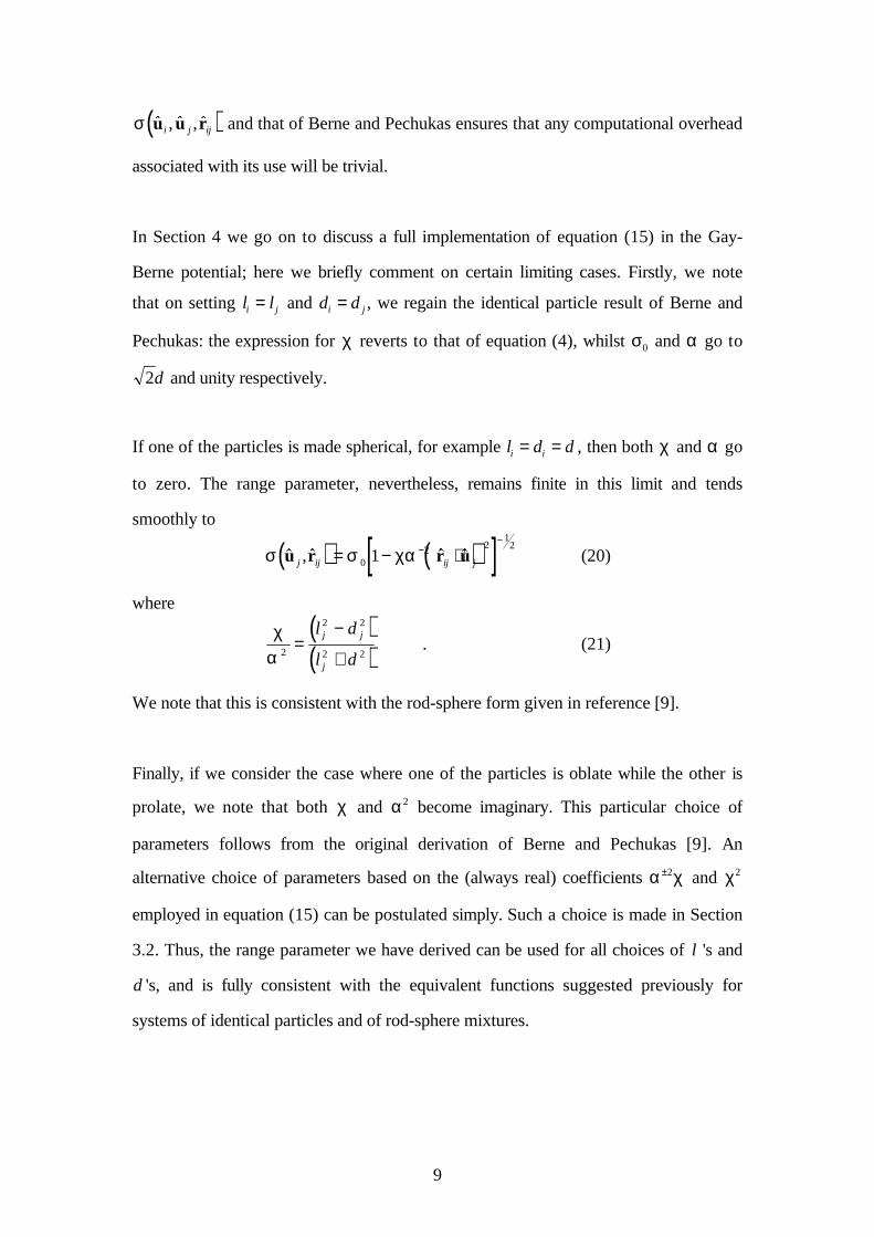
In Section 4 we go on to discuss a full implementation of equation (15) in the Gay-

Berne potential; here we briefly comment on certain limiting cases. Firstly, we note

that on setting l li j= and d di j= , we regain the identical particle result of Berne and

Pechukas: the expression for χ reverts to that of equation (4), whilst σ0 and α go to

2d and unity respectively.

If one of the particles is made spherical, for example l d di i= = , then both χ and α go

to zero. The range parameter, nevertheless, remains finite in this limit and tends

smoothly to

( ) ( )[ ]σ σ χα$ , $ $ $u r r uj ij ij j= − ⋅−−

02 2

12

1 (20)

where

( )( )

χα 2

2 2

2 2=

−

+

l d

l d

j j

j

. (21)

We note that this is consistent with the rod-sphere form given in reference [9].

Finally, if we consider the case where one of the particles is oblate while the other is

prolate, we note that both χ and α 2 become imaginary. This particular choice of

parameters follows from the original derivation of Berne and Pechukas [9]. An

alternative choice of parameters based on the (always real) coefficients α χ±2 and χ2

employed in equation (15) can be postulated simply. Such a choice is made in Section

3.2. Thus, the range parameter we have derived can be used for all choices of l 's and

d 's, and is fully consistent with the equivalent functions suggested previously for

systems of identical particles and of rod-sphere mixtures.

10

3.2 Uniaxial and Biaxial Ellipsoids via the Perram-Wertheim

Route

The route just outlined does not represent the only approach by which to calculate the

uniaxial range parameter. It has been shown by Perram et al. [15] that the range

parameter of Berne and Pechukas' gaussian overlap potential is identical to a simple

approximation of the hard ellipsoid contact function due to Perram and Wertheim [16].

The true overlap function for hard ellipsoids i, j may be written in the form

( ) ( ) ( )F r f r fi j ij ij i j ij ij i j ijPW PW$ , $ , $ , $ , $ max $ , $ , $u u r u u r u u r= =

≤ ≤

2 2

0 1λλ , (22)

where ( )f i j ijPW $ , $ , $u u r and ( )f i j ijλ $ , $ , $u u r depend on particle orientations, not

separations, and ( )f i j ijλ $ , $ , $u u r additionally has a parametric dependence on λ . All of

these functions also depend on the dimensions of the ellipsoids. When

( )F i j ijPW $ , $ ,u u r <1 the two ellipsoids overlap; when ( )F i j ij

PW $ , $ ,u u r >1 they do not;

( )F i j ijPW $ , $ ,u u r =1 is the tangency condition. Explicit expressions for ( )F i j ij

PW $ , $ ,u u r

are given by Perram and Wertheim [16] for the case of general spheroids (not

necessarily identical) and for the special case of identical, axially symmetric, ellipsoids

of revolution. The expression is equivalent to Vieillard-Baron's criterion [19] for

ellipsoid overlap; some discussion of the two approaches, and their use in simulations,

appears elsewhere [2]. Because of the scaling with rij2 evident in the above equation, it

is clear that

( ) ( )σ PW

PW$ , $ , $ $ , $ , $u u r

u u ri j ij

i j ijf≡ 1

(23)

is the distance of closest approach for hard ellipsoids with the specified orientations.

As pointed out in [15], and echoed in [2], ( )σ PW $ , $ , $u u ri j ij reduces to the gaussian

overlap range parameter if λ is set to 1 2, i.e.

( ) ( )σ $ , $ , $ $ , $ , $

u u ru u r

i j ij

i j ijf≡ 1

1 2

. (24)

11

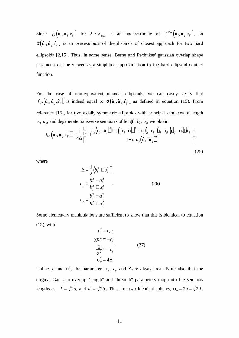
Since ( )f i j ijλ $ , $ , $u u r for λ λ≠ max is an underestimate of ( )f i j ijPW $ , $ , $u u r , so

( )σ $ , $ , $u u ri j ij is an overestimate of the distance of closest approach for two hard

ellipsoids [2,15]. Thus, in some sense, Berne and Pechukas' gaussian overlap shape

parameter can be viewed as a simplified approximation to the hard ellipsoid contact

function.

For the case of non-equivalent uniaxial ellipsoids, we can easily verify that

( )f i j ij1 2 $ , $ , $u u r is indeed equal to ( )σ $ , $ , $u u ri j ij as defined in equation (15). From

reference [16], for two axially symmetric ellipsoids with principal semiaxes of length

ai , a j , and degenerate transverse semiaxes of length bi , bj , we obtain

( ) ( ) ( ) ( )( )( )( )

fc c c c

c ci j ij

x ij i y ij j x y ij i ij j i j

x y i j

1 2

2 2

2

1

41

1$ , $ , $ $ $ $ $ $ $ $ $ $ $

$ $u u rr u r u r u r u u u

u u= +

⋅ + ⋅ + ⋅ ⋅ ⋅

− ⋅

∆

,

(25)

where

( )∆ = +

=−+

=−+

1

22 2

2 2

2 2

2 2

2 2

b b

cb a

b a

cb a

b a

i j

xi i

j i

y

j j

i j

. (26)

Some elementary manipulations are sufficient to show that this is identical to equation

(15), withχ

χαχασ

2

2

2

02 4

=

= −

= −

=

c c

c

c

x y

x

y

∆

. (27)

Unlike χ and α 2, the parameters cx , cy and ∆ are always real. Note also that the

original Gaussian overlap "length" and "breadth" parameters map onto the semiaxis

lengths as l ai i= 2 and d bi i= 2 . Thus, for two identical spheres, σ0 2 2= =b d .

12

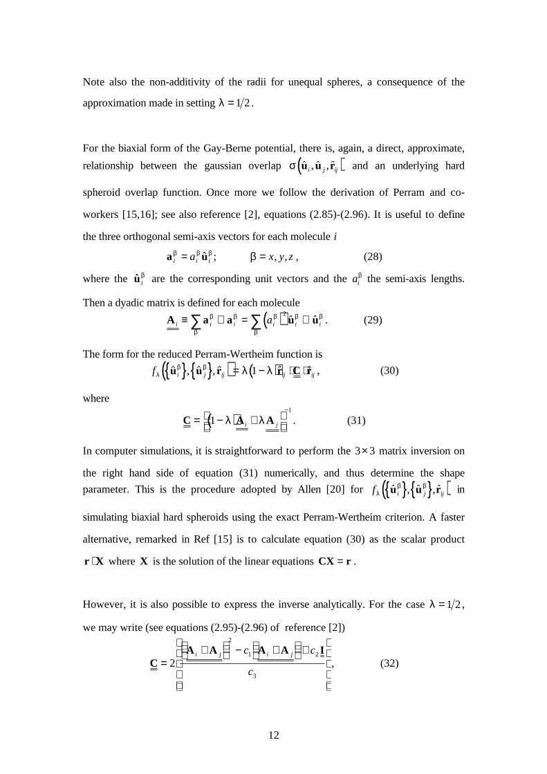
Note also the non-additivity of the radii for unequal spheres, a consequence of the

approximation made in setting λ = 1 2.

For the biaxial form of the Gay-Berne potential, there is, again, a direct, approximate,

relationship between the gaussian overlap ( )σ $ , $ , $u u ri j ij and an underlying hard

spheroid overlap function. Once more we follow the derivation of Perram and co-

workers [15,16]; see also reference [2], equations (2.85)-(2.96). It is useful to define

the three orthogonal semi-axis vectors for each molecule i

a ui i ia x y zβ β β β= =$ ; , , , (28)

where the $u iβ are the corresponding unit vectors and the ai

β the semi-axis lengths.

Then a dyadic matrix is defined for each molecule

( )A a a u ui i i i i ia≡ ⊗ = ⊗∑ ∑β

β

β β β

β

β2 $ $ . (29)

The form for the reduced Perram-Wertheim function is

{ } { }( ) ( )f i j ij ij ijλβ β λ λ$ , $ , $ $ $u u r r C r= − ⋅ ⋅1 , (30)

where

( )C A A= − +

−

11

λ λi j . (31)

In computer simulations, it is straightforward to perform the 3 3× matrix inversion on

the right hand side of equation (31) numerically, and thus determine the shape

parameter. This is the procedure adopted by Allen [20] for { } { }( )f i j ijλβ β$ , $ , $u u r in

simulating biaxial hard spheroids using the exact Perram-Wertheim criterion. A faster

alternative, remarked in Ref [15] is to calculate equation (30) as the scalar product

r X⋅ where X is the solution of the linear equations CX r= .

However, it is also possible to express the inverse analytically. For the case λ = 1 2,

we may write (see equations (2.95)-(2.96) of reference [2])

CA A A A I

=+

− +

+

2

2

1 2

3

i j i jc c

c, (32)

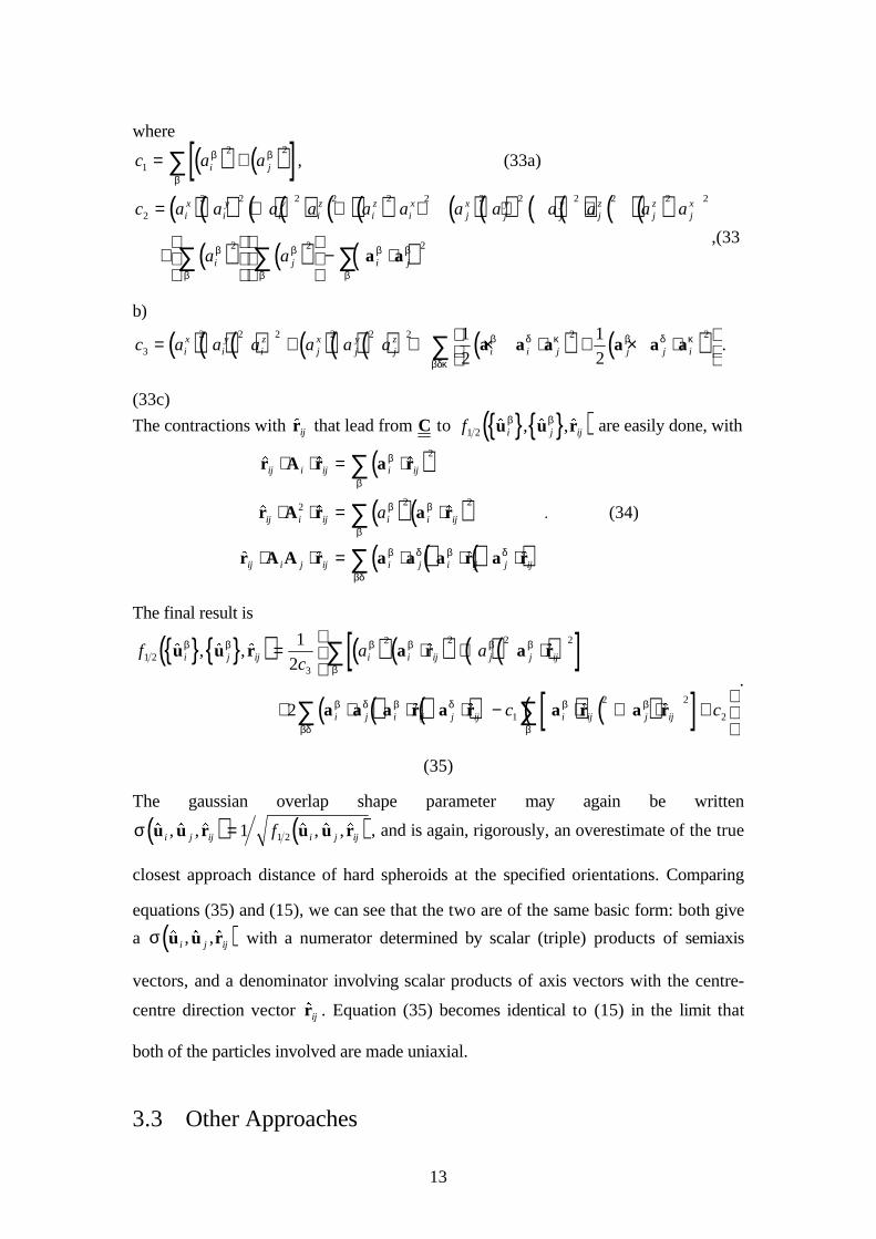
13

where

( ) ( )[ ]c a ai j1

2 2= +∑ β β

β

, (33a)

( ) ( ) ( ) ( ) ( ) ( ) ( ) ( ) ( ) ( ) ( ) ( )( ) ( ) ( )

c a a a a a a a a a a a a

a a

ix

iy

iy

iz

iz

ix

jx

jy

jy

jz

jz

jx

i j i j

2

2 2 2 2 2 2 2 2 2 2 2 2

2 2 2

= + + + + +

+

− ⋅∑ ∑ ∑β

β

β

β

β β

β

a a,(33

b)

( ) ( ) ( ) ( ) ( ) ( ) ( ) ( )c a a a a a aix

iy

iz

jx

jy

jz

i i j j j i3

2 2 2 2 2 2 2 21

2

1

2= + + × ⋅ + × ⋅

∑ a a a a a aβ δ κ β δ κ

βδκ

.

(33c)

The contractions with $rij that lead from C to { } { }( )f i j ij1 2 $ , $ , $u u rβ β are easily done, with

( )

( ) ( )( )( )( )

$ $ $

$ $ $

$ $ $ $

r A r a r

r A r a r

r A A r a a a r a r

ij i ij i ij

ij i ij i i ij

ij i j ij i j i ij j ij

a

⋅ ⋅ = ⋅

⋅ ⋅ = ⋅

⋅ ⋅ = ⋅ ⋅ ⋅

∑

∑

∑

β

β

β β

β

β δ β δ

βδ

2

2 2 2. (34)

The final result is

{ } { }( ) ( ) ( ) ( ) ( )[ ]( )( )( ) ( ) ( )[ ]

fc

a a

c c

i j ij i i ij j j ij

i j i ij j ij i ij j ij

1 23

2 2 2 2

1

2 2

2

1

2

2

$ , $ , $ $ $

$ $ $ $

u u r a r a r

a a a r a r a r a r

β β β β β β

β

β δ β δ β β

ββδ

= ⋅ + ⋅

+ ⋅ ⋅ ⋅ − ⋅ + ⋅ +

∑

∑∑.

(35)

The gaussian overlap shape parameter may again be written

( ) ( )σ $ , $ , $ $ , $ , $u u r u u ri j ij i j ijf=1 1 2 , and is again, rigorously, an overestimate of the true

closest approach distance of hard spheroids at the specified orientations. Comparing

equations (35) and (15), we can see that the two are of the same basic form: both give

a ( )σ $ , $ , $u u ri j ij with a numerator determined by scalar (triple) products of semiaxis

vectors, and a denominator involving scalar products of axis vectors with the centre-

centre direction vector $rij . Equation (35) becomes identical to (15) in the limit that

both of the particles involved are made uniaxial.

3.3 Other Approaches

14

Before closing this Section, we note that we have found another route to equations

(15)-(19) based simply on the behaviour of the shape parameter in the five

configurations shown in Table 1. Following the original result of Berne and Pechukas,

we assumed the shape parameter to be given by a minimally modified form of equation

(3) and took ( )σ $ , $ , $u u ri j ij to be given by the root mean square of the appropriate pair

of li , l j , di and d j for each of the five configurations (e.g. for the side-side

arrangement, taking ( )σ 2 2 20 5= +. d di j ). Whilst this approach is clearly unsatisfactory

in isolation, its success in yielding the correct final expressions demonstrates that the

behaviour of the gaussian overlap range parameter is both simple and intuitive.

Whilst the Perram-Wertheim approach offers the simplest route to ( )σ $ , $ , $u u ri j ij for the

generalised particle shapes we are concerned with here, it lacks clear physical

interpretation. The impact of setting λ = 1 2 is far from obvious, and an interaction

potential based on this approximation is hard to justify until reference is made to the

origins of the gaussian overlap approach.

The ellipsoid contact function itself, ( )f i j ijλ $ , $ , $u u r at λ λ= max , has some advantages

over ( )σ $ , $ , $u u ri j ij , such as its adherence to the Lorentz-Berthelot additivity rule.

However, the crucial point in favour of the latter is its simple analytical form which is

easily differentiable. It can, therefore, be used in molecular dynamics simulations using

‘soft’ interaction potentials (this is not practicable with the ellipsoid contact function

which would require numerical differentiation to calculate each force contribution).

Thus, whilst it may be of interest to perform a Monte Carlo simulation employing the

ellipsoid contact function, ( )σ $ , $ , $u u ri j ij remains a significant and more convenient

alternative.

4 Application to the Gay-Berne Model

15

4.1 The Gay-Berne Strength Parameter

The task of importing the generalised shape parameter into the Gay-Berne potential

involves little more than inserting equations (15-18) into equation (7). However, the

strength anisotropy term of equation (9) also needs to be modified; if it were not then

the well depths for the two different T configurations (see Table 1) would be equal. By

reference to our shape parameter result we suggest use of the form

( ) ( ) ( ) ( )( )( )( )

ε χα α χ

χ2

2 2 2 2

2 212

1$ , $ , $ $ $ $ $ $ $ $ $ $ $

$ $u u rr u r u r u r u u u

u ui j ij

ij i ij j ij i ij j i j

i j

= − ′′ ⋅ + ′ ⋅ − ′ ⋅ ⋅ ⋅

− ′ ⋅

−

,

(36)

where, as previously, we have introduced a single new parameter, ′α . The task of

relating the parameters ε0, µ , ν , ′χ and ′α to the system of interest is rather less clear

cut than that experienced in deriving the shape parameter. As evidence of this, we note

that there are currently a number of different strength anisotropy parameterisations

being used for Gay-Berne systems with identical shape anisotropies [10,21].

In order to gain an indication of how these parameters relate to given configurations,

we list, in Table 1, the form of ( )ε $ , $ , $u u ri j ij for each of the arrangements listed. From

this we see that ε0 is the only relevant parameter for the cross (X) arrangement and

that ν controls the well-depth variation from the cross to the side-side (S)

arrangement.

An initial route to determining the other three parameters is offered by noting that the

expressions given in Table 1 represent a series of simultaneous equations in µ , ′χ and

′α : a numerical solution of these equations should give a suitable starting point for a fit

to a full potential. We stress that this does not represent a rigorous means by which to

16

parameterise a given system, however, and urge that this matter be considered anew

for each new set of l 's and d 's used.

Before attempting such a parameterisation, we note that in the limit of identical

particles, the two T configurations become equivalent, and ′α goes to unity; equation

(36) then reduces to the standard Gay-Berne relationship. Alternatively, if one of the

particles is spherical, then the S, X and, say, T1 arrangements, and the E and T2

arrangements become equivalent. As in the case of the range parameter, both ′χ and

′α then go to zero, whilst the product, ′ ′ −χ α 2, remains finite. Thus, the well depth

anisotropy function becomes

( ) ( )[ ]ε ε χ αµ$ , $ $ $u r r uj ij ij j= − ′ ′ ⋅−

02 2

1 , (37)

where

′ ′ = −

−χ α ε

ε

µ2

1

1 E

S

(38)

and ε εS 0= . For the rod-sphere interaction, the equivalence of the S and X

arrangements requires that ν be zero. The remaining parameters, µ and ′ ′ −χ α 2 (if they

are both to be used) can be obtained from a fit to the full potential.

4.2 Parameterisation of a Rod-Disk Interaction

In seeking a set of parameters suitable for modelling the interaction between a rod-like

particle and a disk-like particle, we have closely followed the procedure used by

Luckhurst et al. in their analyses of the rod-rod and disk-disk parameterisations of the

standard Gay-Berne model [17,11]. This is based on a Boltzmann weighted average of

the interaction between a pair of molecules, calculated purely from the sum of atom-

centred Lennard-Jones interactions. Whilst this procedure has been found to yield

potentials which overestimate the relative well depth ratios of the various

configurations (due to its neglect of molecular flexibility and other important factors

17

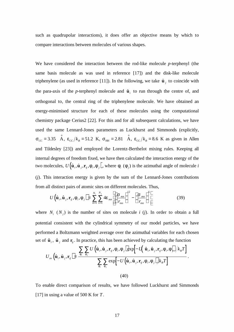
such as quadrupolar interactions), it does offer an objective means by which to

compare interactions between molecules of various shapes.

We have considered the interaction between the rod-like molecule p-terphenyl (the

same basis molecule as was used in reference [17]) and the disk-like molecule

triphenylene (as used in reference [11]). In the following, we take $u j to coincide with

the para-axis of the p-terphenyl molecule and $u i to run through the centre of, and

orthogonal to, the central ring of the triphenylene molecule. We have obtained an

energy-minimised structure for each of these molecules using the computational

chemistry package Cerius2 [22]. For this and for all subsequent calculations, we have

used the same Lennard-Jones parameters as Luckhurst and Simmonds (explicitly,

σCC

o

A= 3 35. , εCC kB = 512. K, σHH

o

A= 2 81. , εCC kB = 8 6. K as given in Allen

and Tildesley [23]) and employed the Lorentz-Berthelot mixing rules. Keeping all

internal degrees of freedom fixed, we have then calculated the interaction energy of the

two molecules, ( )U i j ij i j$ , $ , , ,u u r φ φ , where φi (φj ) is the azimuthal angle of molecule i

(j). This interaction energy is given by the sum of the Lennard-Jones contributions

from all distinct pairs of atomic sites on different molecules. Thus,

( )Ur ri j ij i j mn

mn

mn

mn

mnn

N

m

N ji$ , $ , , ,u u r φ φ ε σ σ=

−

==

∑∑ 412 6

11

(39)

where Ni ( N j ) is the number of sites on molecule i (j). In order to obtain a full

potential consistent with the cylindrical symmetry of our model particles, we have

performed a Boltzmann weighted average over the azimuthal variables for each chosen

set of $u i , $u j and rij . In practice, this has been achieved by calculating the function

( )( ) ( )[ ]

( )[ ]U

U U k T

U k Ti j ij

i j ij i j i j ij i j B

i j ij i j B

ji

ji

av $ , $ ,

$ , $ , , , exp $ , $ , , ,

exp $ , $ , , ,u u r

u u r u u r

u u r=

−

−

∑∑

∑∑φφ

φφ

φ φ φ φ

φ φ.

(40)

To enable direct comparison of results, we have followed Luckhurst and Simmonds

[17] in using a value of 500 K for T .

18

We have calculated ( )U i j ijav $ , $ ,u u r for a range of rij for each of the $u i , $u j , $rij

combinations shown in Table 1. The results of these calculations, which were obtained

using a 1 degree increment in the azimuthal sums of equation (40), are shown as full

lines in Figure 1. We have performed a least squares fit of our model potential to these

data using the NAG minimisation routine E04JAF. This fit is shown as the dashed lines

in Figure 1, and corresponds to the parameter values σ0=7.6 Ao

; ε0 kB =1380 K;

α χ2 =-3.0; χ2=-5.7; µ=3.8; ν=0.13; ′ ′χ α 2=-0.11; ′χ 2=0.46.

From Figure 1, we observe that this fit is quantitatively reasonable throughout. The

properties which relate to the range parameter variables (i.e. the separations at which

the potential first becomes attractive) are matched particularly well. All of the fitted

curves have shallower minima than the corresponding ( )U i j ijav $ , $ ,u u r curves,

indicating that the shifted 12-6 form of the Gay-Berne potential is generally unable to

reproduce the shape of a potential composed of a sum of Lennard-Jones sites. A

related discrepancy is that some of the long ranged tails appear rather too attractive.

Despite this, the relative well depths of four of the five ( )U i j ijav $ , $ ,u u r curves are well

reproduced (the exception is the E curve, which is too shallow).

In their parameterisation of the rod-rod potential, Luckhurst and Simmonds obtained a

well depth ratio ε εS E of 39.6, with ε0 kB = 4302 K [17]. Emerson et al. obtained

ε εE S = 9 for a disk-disk interaction [11] but did not report any absolute values. The

greatest well-depth ratio we have found in our ( )U i j ijav $ , $ ,u u r data is 10.4 (11.4 in our

fitted data), substantially less than the 39.6 found for the two rods. This, along with the

respective ε0 values obtained, supports intuitive arguments that in a mixture of

(similarly sized) rods and disks, the strongest rod-disk interaction will be weaker than

the strongest rod-rod and disk-disk interactions.

19

The value we have obtained for the exponent µ is broadly similar to that used in the

various simulations of identical Gay-Berne particles [10,11,17,21]. Our value for ν is

substantially smaller than that used for such systems, however. Such a difference is to

be expected; the relevant part of the strength anisotropy function, ( )ε1 $ , $u ui j , is itself

much bigger than that used in the identical particle interaction, due to the negative

value of χ2 (recall equations (6) and (8)). Small ν values should, therefore, be a

feature of all rod-disk parameterisations.

The remaining parameters of our fit do not naturally lend themselves to specific

discussion. We note that the (unprimed) shape parameter variables obtained have given

very good agreement with the input data for the specific case considered here. This

supports continued use of potentials based on the gaussian overlap shape parameter.

The main failure of the fit is that it underestimates the relative depth of the E

arrangement. This, along with the general shallowness of the fitted curves may indicate

that an alternative to the shifted 12-6 Gay-Berne potential form may yield closer

agreement to realistic molecule-molecule interactions. This must remain a rather

tentative conclusion, however, given the relatively crude molecular model compared

with in this work.

In conclusion, we have developed a generalised version of the Gay-Berne potential

which enables calculation of the interaction between dissimilar uniaxial or biaxial

particles. This interaction potential reduces to the standard Gay-Berne and Lennard-

Jones forms in the appropriate limits. As such, it is appropriate for use in a number of

simulation systems involving mixtures or assemblies of non-spherical interaction sites.

Acknowledgements

This work arose from discussions held at the meetings of the CCP5-sponsored

complex fluid simulators consortium and the British Liquid Crystal Society in March

20

1994. The authors acknowledge useful conversations with many members of the

former, particularly M.R. Wilson and A.P.J. Emerson. We also thank J.W. Perram for

providing reference [15] and C. Zannoni for communicating details of work in progress

(reference [12]).

21

References

[1] For reviews of this subject see D. Frenkel, Molec. Phys., 60, 1 (1987); M.P.

Allen, Phil. Trans. R. Soc. Lond. A, 344, 323 (1993).

[2] M.P. Allen, G.T. Evans, D. Frenkel and B.M. Mulder, Adv. Chem. Phys., 86, 1

(1993).

[3] M.P. Allen and M.R. Wilson, J. Comput. Aided Mol. Des., 3, 335 (1989); M. P.

Allen, in Observation, prediction and simulation of phase transitions in

Complex Fluids Eds: M. Baus, L. Rull and J.-P. Ryckaert, Proceedings of

International School of Physics "Enrico Fermi" Course CXXIX, Varenna (1994)

(in press).

[4] G.R. Luckhurst and S. Romano, Proc. Roy. Soc. Lond. A, 373, 111 (1980).

[5] M.D. De Luca, M.P. Neal and C.M. Care, Liquid Crystals, 16, 257 (1994); M.P.

Neal, M.D. De Luca and C.M. Care, Mol. Sim., accepted (1994).

[6] G.V. Paoloni, G. Ciccotti and M. Ferrario, Molec. Phys., 80, 297 (1993).

[7] S.J. Picken, W.F. van Gunsteren, P.Th. van Duijnen, and W.H. de Jeu, Liquid

Crystals, 6, 357 (1989); M.R. Wilson and M.P. Allen, Molec. Cryst. Liq. Cryst.,

198, 465 (1991); M.R. Wilson and M.P. Allen, Liquid Crystals, 12, 157 (1992).

[8] J.G. Gay and B.J. Berne, J. chem. Phys., 74, 3316 (1981).

[9] B.J. Berne and P. Pechukas, J. chem. Phys., 64, 4213 (1972).

[10] D.J. Adams, G.R. Luckhurst and R.W. Phippen, Molec. Phys., 61, 1575 (1987);

G.R. Luckhurst, R.W Phippen and R.A. Stephens, Liquid Crystals, 8, 451

(1990); E. De Miguel, L.F. Rull, M.K. Chalam and K.E. Gubbins, Molec. Phys.,

74, 405 (1991); S. Sarman and D.J. Evans, J. chem. Phys., 99, 9021; R. Berardi,

A.P.J. Emerson and C. Zannoni, J. Chem. Soc. Faraday Trans., 89, 4069 (1993).

[11] A.P.J. Emerson, G.R. Luckhurst and S.G. Whatling, Molec. Phys., 82, 113

(1994).

[12] R. Berardi, C. Fava and C. Zannoni, Chem. Phys. Lett. accepted for publication.

[13] P.S.J. Simmonds, Ph.D. Thesis, University of Southampton (1990).

22

[14] A.P.J. Emerson and G.R. Luckhurst, private communication (1994); M.P. Neal,

A.J. Parker and C.M. Care, presented at the 10th BLCS Conference, Exeter

(1995). .

[15] J.W. Perram, E. Praestgaard, J. Rasmussen and J. Lebowitz, preprint (kindly

provided by John Perram).

[16] J.W. Perram and M.S. Wertheim, J. Comput. Phys., 58, 409 (1985).

[17] G.R. Luckhurst and P.S.J Simmonds, Molec. Phys., 80, 233 (1993)

[18] J. Kushick and B.J. Berne, J. chem. Phys., 64, 1362 (1976).

[19] J. Vieillard-Baron, J. chem. Phys., 56, 4729 (1972).

[20] M.P. Allen, Liquid Crystals, 8, 499 (1990).

[21] R. Berardi, A.P.J. Emerson and C. Zannoni, J. chem. Soc. Faraday Trans., 89,

4069 (1993).

[22] Energy minimised single-molecule structures were generated using the program

Cerius2TM . This program was developed by Molecular Simulations Incorporated.

Subsequent generation of ( )U i j ijav $ , $ ,u u r data was performed using in-house

codes.

[23] M.P. Allen and D.J. Tildesley, Computer Simulation of Liquids, (Clarendon,

Oxford, 1989).

23

Table 1: The relative positions and orientations of the five arrangements used to

define the parameters of the well-depth anisotropy function. The figures illustrate the

arrangements for a rod-like particle (molecule j ) and a disk-like particle (molecule i ).

These are differentiated by the marking of symmetry axes.

Figure 1: ( )U i j ijav $ , $ ,u u r data (solid lines) for the azimuthally averaged interaction

potential of p-terphenyl and triphenylene, and associated fit of the generalised Gay-

Berne model (dashed lines). See text for fit parameters. The fits were generated using

data from a limited range of rij values; the upper limit of this range, for each of the

curves shown, is indicated by the vertical discontinuity at large rij .