ANALYTICAL STUDY AND GENERALISATION OF SELECTED

STOCK OPTION VALUATION MODELS

By

EDEKI, SUNDAY ONOS

Matriculation Number: 13PCD00571

JUNE, 2017

ANALYTICAL STUDY AND GENERALISATION OF SELECTED

STOCK OPTION VALUATION MODELS

By

EDEKI, SUNDAY ONOSB.Sc (Ed) Mathematics (Abraka)

M.Sc Mathematics (Ibadan)Matriculation Number: 13PCD00571

A THESIS SUBMITTED TO THE DEPARTMENT OF

MATHEMATICS, COLLEGE OF SCIENCE AND TECHNOLOGY,

COVENANT UNIVERSITY, OTA, IN PARTIAL FULFILLMENT OF

THE REQUIREMENTS FOR THE AWARD OF Ph.D DEGREE IN

INDUSTRIAL MATHEMATICS

JUNE, 2017

ii

ACCEPTANCE

This is to attest that this thesis is accepted in partial fulfillment for the award of

the degree of Doctor of Philosophy in Industrial Mathematics, College of Science and

Technology, Covenant University, Ota.

Philip John Ainwokhai . . . . . . . . . . . . . . . . . . . . . . . . . . . . . . .

(Secretary, School of Postgraduate Studies) Signature & Date

Professor Samuel T. Wara . . . . . . . . . . . . . . . . . . . . . . . . . . . . . .

(Dean, School of Postgraduate Studies) Signature & Date

iii

DECLARATION

I, EDEKI Sunday Onos (13PCD00571) declare that this research was carried out

by me under the supervision of Professor (Mrs) Olabisi O. Ugbebor of the Department

of Mathematics, University of Ibadan, Ibadan, Oyo State, Nigeria and Dr. Enahoro A.

Owoloko of the Department of Mathematics, Covenant University, Ota, Ogun State,

Nigeria. I attest that this thesis has not been presented either wholly or partially for

the award of any degree anywhere else. All the sources of data, scholarly publications

and information used in this thesis are cited and acknowledged accordingly.

. . . . . . . . . . . . . . . . . . . . . . . . . . . . . . . . . . . . . . .EDEKI Sunday Onos

(Student) Signature & Date

iv

CERTIFICATION

We certify that this thesis titled “Analytical Study and Generalisation of Selected

Stock Option Valuation Models” is an original work carried out by Sunday Onos

EDEKI (13PCD00571) in the Department of Mathematics, College of Science and

Technology, Covenant University, Ota, Ogun State, Nigeria, under the supervision

of Professor Olabisi O. Ugbebor and Dr. Enahoro A. Owoloko. We have examined

and found the work acceptable as part of the requirements for the award of Doctor of

Philosophy (Ph.D) degree in Industrial Mathematics.

. . . . . . . . . . . . . . . . . . . . . . . . . . . . . . . . . . . .Professor Olabisi O. Ugbebor

(Supervisor) Signature & Date

. . . . . . . . . . . . . . . . . . . . . . . . . . . . . . . . . . . . .Dr. Enahoro A. Owoloko

(Co-Supervisor) Signature & Date

. . . . . . . . . . . . . . . . . . . . . . . . . . . . . . . . . .Dr. Timothy A. Anake

(Head of Department) Signature & Date

. . . . . . . . . . . . . . . . . . . . . . . . . . . . . . . . . . . . . .Professor Sunday J. Kayode

(External Examiner) Signature & Date

. . . . . . . . . . . . . . . . . . . . . . . . . . . . . . . . .Professor Samuel T. Wara

(Dean, School of Postgraduate Studies) Signature & Date

v

DEDICATION

To the Almighty God for wisdom, knowledge, provision and protection.

vi

ACKNOWLEDGEMENTS

I sincerely appreciate the Almighty God for divine grace, knowledge, wisdom, protec-

tion and all round provision throughout this programme.

I remain indebted and grateful to the Chancellor, Dr. David O. Oyedepo, through

whom this platform was created.

I am indeed grateful to the current Vice Chancellor, Prof. AAA. Atayero, the im-

mediate past Vice Chancellor, Prof. C. K. Ayo, and the entire management team of

Covenant University, Ota for their support, provision of good working environment,

and encouragement.

My appreciation and gratitude go to my Supervisor, Prof. (Mrs.) O. O. Ugbebor, for

her invaluable contribution, encouragement, motherly advice, support and guidance

throughout the period of this research work. She was also my supervisor at the

Masters level; I therefore, say with all sincerity that her style of mentoring, and

wealth of knowledge are indeed worthy of emulation. God bless you Ma.

I am also grateful to my Co-Supervisor, Dr. E. A. Owoloko, for his useful comments,

suggestions, encouragement and advice. His advocacy of possibility mentality has

indeed been helpful.

I appreciate the effort of the Ag. Head, Department of Mathematics, Dr. T. A. Anake

for useful suggestions, and quality drive at all time.

I frankly extend my appreciation to members of the post-graduate committee of the

Department of Mathematics, Covenant University, Ota who have in one way or the

other rendered meaningful suggestions to me during the course of this research work.

I will also not fail to mention the invaluable assistance of my colleagues in the De-

vii

partment of Mathematics especially the valuable comments and criticisms during the

seminar presentations. Notable among them are Prof. S. A. Iyase, Dr. A. S. Idowu,

Dr. S. A. Bishop (the PG Coordinator), Dr. M. O. Adamu, and Dr. A. O.

Adejumo. My special thank also goes to Mrs. G. O. Alao for the draft editing, and

Mr. O. J. Adeleke for the installation and guidance on LaTeX software package.

I am also thankful to Mrs. I. Adinya, Mr. A. O. Akeju, and Dr. T. A. Anake through

whom I got to know of the opportunity available in Covenant University. They are

indeed more than friends and colleague.

I am grateful to my lecturers, co-mathematicians, and friends in other prominent

institutions; these include Prof. E. O. Ayoola, Prof. G. O. S. Ekhaguere (who intro-

duced me to Financial Mathematics), Dr. O. S. Obabiyi, Mr A. O. Akeju, Mrs. I.

Adinya, Mrs. M. E. Adeosun, to mention but a few.

My sincere thanks go to the following Examiners: Dr. A. P. Aizebeokhai (Department

of Physics), Dr. O. J. Oyelade (Department of Computer and Information Sciences),

and Dr. O. A. Adegbuyi (Department of Business Management), all of Covenant

University, Ota, for their useful suggestions and comments at the proposal stage of

this work.

I am very much indebted to my late parents: Pa S. A. Edeki Ogbomo and Mrs Bethel

Edeki through whom God brought me to this wonderful world. In a similar way,

my heartfelt thanks go to my relatives, brothers and sisters for their support and

understanding.

Finally but not the least, I am indebted to my beloved wife, Mrs V. O. Edeki, for

her wonderful support, understanding, and patience throughout the period of this

research work.

viii

TABLE OF CONTENTS

i

ii

iii

iv

v

vi

vii

ix

xiv

xv

xvi

xviii

xxi

COVER PAGE

TITLE PAGE

ACCEPTANCE

DECLARATION

CERTIFICATION

DEDICATION

ACKNOWLEDGEMENTS

TABLE OF CONTENT

LIST OF TABLES

LIST OF FIGURES

LIST OF SYMBOLS

LIST OF ABBREVIATIONS

ABSTRACT

CHAPTER ONE: INTRODUCTION 1

1.1 Background to the Study . . . . . . . . . . . . . . . . . . . . . . . . . 1

1.2 Statement of the Problem . . . . . . . . . . . . . . . . . . . . . . . . 5

1.3 Aim and Objectives . . . . . . . . . . . . . . . . . . . . . . . . . . . . 6

1.4 Justification of the Study . . . . . . . . . . . . . . . . . . . . . . . . . 7

ix

1.5 Significance of the Study . . . . . . . . . . . . . . . . . . . . . . . . . 8

1.6 The Scope of the Study . . . . . . . . . . . . . . . . . . . . . . . . . . 8

1.7 Limitation of the Study . . . . . . . . . . . . . . . . . . . . . . . . . 9

1.8 Structure of the Thesis . . . . . . . . . . . . . . . . . . . . . . . . . . 9

CHAPTER TWO: LITERATURE REVIEW 10

2.1 Introduction . . . . . . . . . . . . . . . . . . . . . . . . . . . . . . . . 10

2.2 Non-Stochastic Models for Stock Prices . . . . . . . . . . . . . . . . . 10

2.3 Stochastic Models for Stock Prices . . . . . . . . . . . . . . . . . . . 12

2.4 Approximate-analytical Methods of Solutions . . . . . . . . . . . . . 18

2.5 Differential Transformation Method (DTM) and its Modification . . . 19

CHAPTER THREE: METHODOLOGY 29

3.1 Introduction . . . . . . . . . . . . . . . . . . . . . . . . . . . . . . . . 29

3.2 Basic Definitions . . . . . . . . . . . . . . . . . . . . . . . . . . . . . 29

3.3 Ito Approach to Stochastic Differential Equations (SDEs) . . . . . . . 34

3.4 Analysis of the Basic Methods . . . . . . . . . . . . . . . . . . . . . . 35

3.4.1 Some Basic Properties of the Differential Transform Method . 36

3.4.2 The Overview of the Modified DTM (MDTM) . . . . . . . . . 37

3.4.3 Some Fundamental Properties and Features of the MDTM . . 37

3.4.4 Overview of the He’s Polynomial . . . . . . . . . . . . . . . . 38

3.4.5 Fractional Calculus: The Preliminary . . . . . . . . . . . . . . 39

3.4.6 Modified Differential Transform (MDT) of a Function with Frac-

tional Derivative . . . . . . . . . . . . . . . . . . . . . . . . . 41

3.4.7 Overview of a Local Fractional PDTM . . . . . . . . . . . . . 42

3.5 Sources of Data: NGSE (2016) and NGSEINDX (2016) . . . . . . . . 43

3.6 The Transformed Black-Scholes Pricing Model . . . . . . . . . . . . . 43

x

3.6.1 The Model Assumptions . . . . . . . . . . . . . . . . . . . . . 44

3.6.2 Derivation of the Transformed Black-Scholes Model . . . . . . 44

CHAPTER FOUR: RESULTS AND DISCUSSION 48

4.1 Introduction . . . . . . . . . . . . . . . . . . . . . . . . . . . . . . . . 48

4.2 The Theoretical Solution of the Transformed Black-Scholes Model . . 48

4.2.1 The DTM Applied to the Transformed Black-Scholes Model

(TBSM) . . . . . . . . . . . . . . . . . . . . . . . . . . . . . . 53

4.2.2 Numerical Calculations and the Transformed Black-Scholes Model 53

4.3 The Generalised Black-Scholes Model via the CEV Stochastic Dynam-

ics . . . . . . . . . . . . . . . . . . . . . . . . . . . . . . . . . . . . . 56

4.3.1 Constant Elasticity of Variance Option Pricing Model: A Case

of no Dividend Yield . . . . . . . . . . . . . . . . . . . . . . . 56

4.3.1.1 Comparison of the Models: The Black-Scholes Model

and the CEV-Black-Scholes Model . . . . . . . . . . 58

4.3.1.2 A Note on Elasticity and Elasticity Parameter . . . . 60

4.3.2 The CEV - Black-Scholes Model on a Basis of Dividend Yield 61

4.3.2.1 The Generalised CEV-Black-Scholes Model on the Ba-

sis of Dividend Yield Parameter . . . . . . . . . . . . 62

4.3.2.2 The CEV-Black-Scholes Model with Parameter Esti-

mation . . . . . . . . . . . . . . . . . . . . . . . . . . 64

4.4 Analytical Solution of the Black-Scholes Model for European Option

Valuation . . . . . . . . . . . . . . . . . . . . . . . . . . . . . . . . . 66

4.4.1 The MDTM Applied for Analytical Solution of Black-Scholes

Pricing Model for European Option Valuation . . . . . . . . . 67

4.4.2 He’s Polynomials Applied to the Black-Scholes Pricing Model

for Stock Option Valuation . . . . . . . . . . . . . . . . . . . . 74

xi

4.4.2.1 The Pricing Model and the He’s Polynomial . . . . . 74

4.5 The Time-Fractional Black-Scholes Option Pricing Model on No-Dividend

Paying Equity . . . . . . . . . . . . . . . . . . . . . . . . . . . . . . . 79

4.5.1 Illustrative Examples and Applications . . . . . . . . . . . . . 79

4.6 The Generalised Bakstein and Howison Model . . . . . . . . . . . . . 95

4.6.1 The Generalisation Procedures . . . . . . . . . . . . . . . . . 95

4.6.1.1 The MDTM Applied to the Generalised Nonlinear Model 98

4.6.1.2 Numerical Illustration and Applications . . . . . . . 100

4.6.2 The Time-Fractional Generalised Bakstein and Howison Model 110

4.6.2.1 The MDTM and the Extended Nonlinear Model . . . 110

4.6.2.2 Numerical Illustration and Applications . . . . . . . 113

4.7 Discussion and Summary of Results . . . . . . . . . . . . . . . . . . . 121

4.7.1 The Transformed Black-Scholes Model . . . . . . . . . . . . . 122

4.7.2 The Generalised Black-Scholes Model . . . . . . . . . . . . . . 124

4.7.2.1 Comparison of the SDE Models (BSM and CEV-BSM) 124

4.7.3 Cases of the Generalised Bakstein and Howison Model - Section

4.6.1 . . . . . . . . . . . . . . . . . . . . . . . . . . . . . . . . 125

4.7.4 The Generalised Bakstein and Howison Model: Time-fractional

case - Section 4.6.2 . . . . . . . . . . . . . . . . . . . . . . . . 128

CHAPTER FIVE: CONCLUSION AND RECOMMENDATIONS 135

5.1 Introduction . . . . . . . . . . . . . . . . . . . . . . . . . . . . . . . . 135

5.2 Conclusion . . . . . . . . . . . . . . . . . . . . . . . . . . . . . . . . . 135

5.3 Contributions to Knowledge . . . . . . . . . . . . . . . . . . . . . . . 137

5.4 Recommendations . . . . . . . . . . . . . . . . . . . . . . . . . . . . . 138

5.5 Open Problems . . . . . . . . . . . . . . . . . . . . . . . . . . . . . . 138

xii

REFERENCES 140

APPENDIX A: MAPLE CODE FOR FIGURES 151

APPENDIX B: NGSEINDX Simulated Data 159

xiii

LIST OF TABLES

Table 4.1 The solutions of case 4.6.1.2.2 at time t = 0 . . . . . . . . . . . . . 107

Table 4.2 The solutions of case 4.6.1.2.2 at time t = 0.5 . . . . . . . . . . . 108

Table 4.3 The solutions of case 4.6.1.2.2 at time t = 1 . . . . . . . . . . . . . 109

Table 4.4 The solutions of case 4.6.3.2.1 at t = 0, α = 1 . . . . . . . . . . 116

Table 4.5 The exact solutions of case 4.6.3.2.1 at t = 0.5, α = 1 . . . 117

Table 4.6 The solutions of case 4.6.3.2.2 at t = 0.5, α = 0.5 . . . . . . . 118

Table 4.7 The solutions of case 4.6.3.2.2 at t = 0.5, α = 1.5 . . . . . . . 119

Table 4.8 The solutions of case 4.6.3.2.2 at t = 1, α = 2.5 . . . . . . . . . 120

Table 4.9 The solutions of the transformed Black-Scholes model . . . 123

xiv

LIST OF FIGURES

Figure 3.1 Simulated Geometric Brownian Motion (GBM). . . . . . . . . 32

Figure 4.1 The Transformed Black-Scholes Model solution in 2-D. . 55

Figure 4.2 Estimates of the CEVM distribution . . . . . . . . . . . . . . . . . . . 65

Figure 4.3 The approximate solution for example 4.4.1.2 . . . . . . . . . . 72

Figure 4.4 The exact solution for example 4.4.1.2 . . . . . . . . . . . . . . . . 73

Figure 4.5 The exact solution of problem 4.4.2.1.1 . . . . . . . . . . . . . . . . 77

Figure 4.6 78

Figure 4.7 89

Figure 4.8 90

Figure 4.9

The approximate solution of problem 4.4.2.1.1 . . . . . . . . .

Contingent Claim Value of problem 4.5.1.1 at t ∈ [0, 9]. . .

Contingent Claim Value of problem 4.5.1.1 at t ∈ [0, 18]. .

Contingent Claim Value of problem 4.5.1.2 at t ∈ [0, 45]. . 91

Figure 4.10 Contingent Claim Value of problem 4.5.1.2 at t ∈ [0, 80]. . 92

Figure 4.11 Contingent Claim Value of problem 4.5.1.3, x ∈ [0, 200]. . 93

Figure 4.12 Contingent Claim Value of problem 4.5.1.3, x ∈ [0, 400]. . 94

Figure 4.13 Approximate solution for Case 4.6.1.2.1 . . . . . . . . . . . . . . 103

Figure 4.14 Exact solution for Case 4.6.1.2.1 . . . . . . . . . . . . . . . . . . . . . 104

Figure 4.15 Exact solution for Case 4.6.1.2.2 . . . . . . . . . . . . . . . . . . . . . . 126

Figure 4.16 Approximate solutions for Case 4.6.1.2.2. . . . . . . . . . . . . . 127

Figure 4.17 Solutions of Case 4.6.3.2.1 using Table 4.4 . . . . . . . . . . . . 129

Figure 4.18 Solutions of Case 4.6.3.2.1 using Table 4.5 . . . . . . . . . . . . 130

Figure 4.19 Solutions of Case 4.6.3.2.2 using Table 4.6 . . . . . . . . . . . . 131

Figure 4.20 Solutions of Case 4.6.3.2.2 using Table 4.7 . . . . . . . . . . . . 132

Figure 4.21 Solutions of of Case 4.6.3.2.2 using Table 4.8 . . . . . . . . . 133

xv

LIST OF SYMBOLS

Symbol Description

St Stock price process at time t

Wt Standard Brownian Motion

σ Stock price volatility

µ Drift parameter (mean rate of return)

V (S, t) Value of an option in stock at time t

r Risk-free interest rate

C1,2 (R+ × [0, T ]) The set of all continuous functions which are once differen-

tiable w.r.t. the first variable and twice differentiable w.r.t.

the second variable

pf (S, t) Payoff function on a stock, S, at time t

t Time parameter

E Expiration price

ξ Rate of elasticity

ρ The constant measuring the liquidity in an illiquid market_σ Volatility function in Bakstein and Howison model

Ω A non-void set

B A σ − algebra of subsets of Ω(Ω, B

)A measurable space(

Ω, B, u∪u)

A measure space(Ω, B,

...

P)

A probability space...

P The real world probability measure(Ω, B,

...

P , F(

B))

A filtered probability space

F(

B)

A filtration

X∗t (ω) A collection of random variables defined on the same prob-

ability space(

Ω, B,...

P)

xvi

E (X∗) Mathematical expectation of the random variable X∗

V ar (X∗) The variance of the random variable X∗

w (·) A differentiable function

W (k) The differential transform of w (·)

Θ(t) A delta-hedge-portfolio

Λ(S, t) Contingent claim value (CCV)

Λ (St, kt) An investment output

kt The total investment (assumed constant), all over a short

period of time, t

pr∗ Production rate

cr∗ Consumption rate

Ξ (S, t) Option value at no dividend yield

ΛoBSM The compared volatility of the Black-Scholes model

ΛoCEVM The compared volatility of the CEV model

ΛrBSM The compared variance of the Black-Scholes model

ΛrCEVM The compared variance of the CEV model

xvii

LIST OF ABBREVIATIONS

Abbreviations Full Meaning

ADM Adomian Decomposition Method

ANNM Artificial Neural Networks Models

Approx Approximate

ARIMA Autoregressive Integrated Moving Average

BICGSTABM Bi-Conjugate Gradient Stabilized Method

BSM Black-Scholes Model

CCV Contingent Claim Value

CEV Constant Elasticity of Variance

CEVM Constant Elasticity of Variance Model

CEV-BSM Constant Elasticity of Variance Black-Scholes Model

COPs Constrained Optimization Problems

DTM Differential Transformation Method

EMH Efficient Market Hypothesis

EMM Equivalent Martingale Measure

ESN Echo State Networks

ESO Employee Stock Option

FBM Fractional Brownian Motion

FDE Fractional Differential Equation

FTBSE Fractional Type Black-Scholes Equation

FTBSM Fractional Type Black-Scholes Model

FVIM Fractional Variation Iterative Method

G-SIM Gauss-Seidel Iterative Method

GBM Geometric Brownian Motion

GMRESM Generalized Minimal Residual Method

HAM Homotopy Analysis Method

HPM Homotopy Perturbation Method

xviii

HPT He’s Polynomial Technique

HPSTM Homotopy Perturbation Sumudu Transform

JIM Jacobi Iterative Method

LADM Laplace Adomian Decomposition Method

LCPs Linear Complementarity Problems

LLWHM Laplace Legendre Wavelet Hybrid Method

MADM Modified Adomian Decomposition Method

MDTM Modified Differential Transformation Method

MHD Magneto-Hydrodynamic

MsDTM Multi-step DTM

MT Mellin Transformation

MVIM Modified Variation Iterative Method

NGSE Nigerian Stock Exchange

NGSEINDX Nigerian Stock Exchange All Share Index

NLFDE Nonlinear Fractional Differential Equation

OTC Over-the-Counter

PCGM Preconditioned Conjugate Gradient Method

PDE Partial Differential Equation

PDT Projected Differential Transform

PDTM Projected Differential Transformation Method

PPM Power Penalty Method

Ref. Reference

Rel. error Relative error

RHPM Revised Homotopy Perturbation Method

R-FIR Risk-free Interest Rate

R-IIR Risk-include Interest Rate

SDE Stochastic Differential Equation

SMI Stock Market Index

STM Sumudu Transform Method

xix

SOR Successive Over Relaxation

TFBSM Time-fractional Black-Scholes Model

VIM Variation Iterative Method

w.r.t. With respect to

xx

ABSTRACT

In this work, the classical Black-Scholes model for stock option valuation on the

basis of some stochastic dynamics was considered. As a result, a stock option val-

uation model with a non-fixed constant drift coefficient was derived. The classical

Black-Scholes model was generalised via the application of the Constant Elasticity of

Variance Model (CEVM) with regard to two cases: case one was without a dividend

yield parameter while case two was with a dividend yield parameter. In both cases,

the volatility of the stock price was shown to be a non-constant power function of

the underlying stock price and the elasticity parameter unlike the constant volatility

assumption of the classical Black-Scholes model. The Ito’s theorem was applied to

the associated Stochastic Differential Equations (SDEs) for conversion to Partial Dif-

ferential Equations (PDEs), while two approximate-analytical methods: the Modified

Differential Transformation Method (MDTM) and the He’s Polynomials Technique

(HPT) were applied to the Black-Scholes model for stock option valuation; in both

cases the integer and time-fractional orders were considered, and the results obtained

proved the latter as an extension of the former. In addition, a nonlinear option pric-

ing model was obtained when the constant volatility assumption of the classical linear

Black-Scholes option pricing model was relaxed through the inclusion of transaction

cost (Bakstein and Howison model). Thereafter, this nonlinear option pricing model

was extended to a time-fractional ordered form, and its approximate-analytical solu-

tions were obtained via the proposed solution technique. For efficiency and reliability

of the method, two cases with five examples were considered: Case 1 with two ex-

amples for time-integer order, and Case 2 with three examples for time-fractional

order, and the results obtained show that the time-fractional order form generalises

the time-integer order form. Thus, the Black-Scholes and the Bakstein and Howison

models for stock option valuation were generalised and extended to time-fractional

order, and analytical solutions of these generalised models were provided.

Keywords: Stock options, Stochastic differential equations, Option valuation, Ana-

lytical solutions , Fractional calculus, Approximate-analytical methods.

xxi

CHAPTER ONE

INTRODUCTION

1.1 Background to the Study

In contemporary financial settings, the role of options in pricing theory is of immense

importance as they can be used for risk control and asset hedging. Stock as a basic

term refers to a company’s assets held by an individual or group in the form of

shares. The accountants view stock from two perspectives: as goods on hand to be

sold to customers (inventory), and as ownership shares of a corporation. A stock

certificate is provided as an evidence of the corporation’s common stock (ordinary

shares) or preferred stock owner thereby making the stockholders partial owners of

the company. Stocks are usually quoted and traded on stock-exchange market. This

transaction entails a financial contract known as derivative security (contingent claim)

whose value at expiration date is derived from the price process of one or some of the

underlying assets (stocks) (Nelson, 1904).

Buying or selling of stocks (shares) in this direction is optional. Hence, an option

is defined as a derivative security furnishing its holder(s) the right (but not an obli-

gation), to make a transaction at a specified period for a specified price. Different

types of options exist (see Sprenkle, 1964; Fama, 1965; Merton, 1973) and these can

be classified in various ways according to the option rights, option styles, underlying

assets and so on. Different types of options are described below.

It is a call (or put) option if associated with a buyer (or seller). The timing for the

exercise of an option defines its style. It is a European option if it can be exercised

only at maturity date while it is an American option if the exercise can be done on

1

or before the maturity date, else such option expires worthless and its existence as

financial instrument ceases. Most exchange traded options follow the American-style

of option.

Other kinds of options include the Asian option whose final asset price (payoff) is

taken as the average of the underlying asset over a predetermined period of time; Asian

option is similar to the European option but differs in terms of the final underlying

values. Barrier option is an option with a general feature indicating that the price

of the underlying security must cross a certain level (barrier) before an exercise can

be done. Look back options are options whose payoffs depend on the maximum or

the minimum of the underlying asset price during some predetermined period. As

the name implies, a look back option allows its holder to ‘look back’ over a specified

period to determine the payoff.

A Swap option or Swaption is a type of option involving two investors with an under-

taking to exchange, at a known date in the future, various financial assets according

to a prearranged formula that depends on the value of one or more underlying assets.

This includes currency swaps and interest rate swaps. In swaption, both the buyer

and the seller agree on the price (premium) of the swaption, and the length of the

period.

A Binary option, also known as ‘all or nothing’ option, allows the payment of the

full amount of payoff if the underlying security meets the specified condition upon

expiration, otherwise its value is worthless. An Exchange Traded option also referred

to as listed option is a type of option traded or listed on a public or regulated trading

exchange. This option can be bought or sold by anybody via the services of an

appropriate broker. It is a standardized contract such that quantity, underlying asset,

date of expiration and strike price are known in advance.

2

On the other hand, Over-the-Counter (OTC) options are options traded in a kind of

market called OTC. The concerned investors who invariably do not meet are linked by

telephones or electronic connectivity. Options on OTC are less accessible to the gen-

eral public since they are not traded on exchanges and the terms are more customized

and complicated than most exchange traded contracts.

Stock option is therefore defined as the right but not an obligation either to buy or sell

stock at a specified price within a stated period of time. Stock option is an example of

option whose underlying assets are shares or stocks. It can also be viewed as benefit

granted to an employee by the employer or company in the form of an option to

purchase the company’s stock at a discounted or fixed price. This is commonly called

Employee Stock Option (ESO); it can serve as a financial assistance at a time of need.

A Stock Index or Stock Market Index (SMI) is a measurement of the value of a

section of stock market. It is computed from the values of selected stocks, usually as

a weighted average. SMI is a tool used by investors to describe the market, and to

compare returns on specific investment.

An option is beneficial because it protects stock holdings from a decline in market

price, helps to increase income against current stock holdings, prepares investors to

buy stock at lower prices, helps investors to position themselves for a big market

move; even without knowing the way prices will move, and helps investors to benefit

from a stock price’s rise or fall without incurring the cost of buying or selling the

stock outright.

In modern finance, the importance of options in pricing theory cannot be overem-

phasized as they can be used for asset hedging, and to control risk. This calls for

the attention of financial engineers when dealing with finance, actuarial sciences, and

other related areas of applied sciences (Habib, 2011).

3

Investors purchase stocks with the hope that the stocks will appreciate in values and

in return, yield income from dividends. Companies or individuals can therefore make

a lot of money via stock trading if the market is well understood. Similarly, it can

also be a huge risk to investors if proper decision is not taken.

One of the highly volatile variables in stock exchange is the stock price. Its unstable

property calls for concern on the investors’ part, since sudden change in share prices

happens frequently and randomly. Researchers are therefore challenged to consider

in their studies the behaviour of this unstable stock parameter in order to render

valuable advice to stock investors and owners of corporation, hence, the importance

of the study of stock options.

The determinants of the value of stock are the forces of supply and demand. Investors

are more concerned with companies’ stocks expected to yield significant profits in the

future. Thus, investment into stocks requires the minimization or control of risk

caused by decrease in stock values.

An efficient way to handle this is the adoption of mathematical model(s) that can

give clear suggestions about the future behaviour of stock prices. Although, there

are market laws such as Efficient Market Hypothesis (EMH) for market transparency,

(Fama, 1970). This EMH gives the same information regarding certain stock to

everyone. Based on EMH, the basic information in relation to the stocks is their

current value since the past price values say nothing about the future behaviour of

the future values. This implies that stock price modelling is geared towards modelling

new information about the concerned stocks.

In financial economy, uncertain movements of stock values over time reflects the dy-

namics of the stock prices. The EMH is one of the reasons for the random movement

of stock prices. The EMH states that the present prices of the stock fully reflect the

4

past history of its prices, and that the market is easily affected by any new information

about the stock. EMH based its assumption on the premise that stock price changes

are Markovian in nature; indicating that the expected future value of stocks depends

only on its current value. Thus, predictions can only be expressed as probability dis-

tribution because of their uncertainty. That is, prediction of the future price of stock

can be done to a certain level of precision if new information about the stock can be

anticipated.

The random nature of the stock price process exhibits the same behaviour as a stochas-

tic process known as Brownian motion. This means that some properties of the stock

price process are traceable to those of Brownian motion process leading to stochastic

modelling of stock prices; since stochastic models are built on random walks, and

are often used in theoretical studies because of their simplicity as only the volatility

parameter is required (Reiss, 1975). In financial mathematics, trading in an illiquid

market in which stock option is an example of illiquid asset has become a topic of

great concern to risk managers and hedgers, since assets in such a market cannot be

exchanged or traded easily for cash without at least a minimal loss of value.

1.2 Statement of the Problem

Models with regard to drift coefficient and volatility parameters have been noted in

literature for option valuation and pricing. The simplest among these with a bearing

from the classical Black-Scholes model for option valuation assumes constant (fixed)

mean rate of return and volatility. However, it is obvious that the constant nature

of these parameters cannot fully explain observed market prices for option valuation

unless when modified (Cen and Le, 2011).

The classical Black-Scholes model for stock price valuation is linear, based on the

5

assumptions that both drift and volatility parameters are constants. In most cases,

relaxing these assumptions results to nonlinear models (Bakstein and Howison, 2003).

The nonlinear transaction-cost model has not been considered in terms of fractional

order but for integer ordered form. In most cases, exact solutions of nonlinear models

do not exist; even when they do, obtaining them via direct solution or conventional

methods seems to possess some setbacks such as linearization, perturbation, compu-

tational time consumption and so on. Therefore, because of the nonlinearity there is

need for reliable, effective and efficient approximate-analytical method(s).

This research is therefore, motivated to address these gaps by developing a stock

option model whose mean rate of return is a non-fixed parameter, generalise the

Black-Scholes model for the inclusion of non-constant volatility, and provide ana-

lytical solutions to the linear and nonlinear stock option models resulting from the

generalisation(s) based on the associated stochastic dynamics.

The application of fast convergent approximate-analytical methods: Modified Dif-

ferential Transformation Method (MDTM) and the Revised Homotopy Perturbation

Method (RHPM) for solving any form of the above models resulting from Stochastic

Differential Equations (SDEs) have not been reported in literature to the best of our

knowledge.

1.3 Aim and Objectives

The aim of this research work is to study and generalise the classical Black-Scholes,

and the Bakstein and Howison pricing models for stock option valuation, and to obtain

approximate-analytical solutions of the models resulting from their associated SDEs.

The objectives of this research work are to:

(i) derive stock option valuation model that will incorporate the drift coefficient

6

(rate of return) as a non-fixed constant without excluding the other parameters

(the risk-free interest rate, and the volatility term;

(ii) obtain a solution for the proposed model in (i) using approximate-analytical

methods;

(iii) generalise the Black-Scholes option pricing model via a constant elasticity of

variance in order to address the assumption of the constant volatility rate in the

Black-Scholes Option Pricing Model;

(iv) determine analytical solutions of European option pricing models via the MDTM

and the RHPM;

(v) generalise the nonlinear transaction cost model of Bakstein and Howison (2003)

for stocks valuation to a time-fractional order form; and

(vi) obtain an analytical solution of the time-fractional generalised Bakstein and

Howison model for stock option valuation in (v).

Note: Throughout this thesis, the term ‘fixed constant’ will be used to denote a

constant that is being suppressed.

1.4 Justification of the Study

The uncertainty in the movement of stock values over time simply reflects the dynamic

nature of the stock prices. This follows a stochastic process known as diffusion process.

The classical Black-Scholes model for option pricing was based on some assumptions

such as constant mean rate of return, and constant volatility. These assumptions could

be relaxed by using the Constant Elasticity of Variance (CEV) stochastic dynamics.

In addition, there is need for the generalisation of the Baskstein and Howison model

induced by CEV to a time-fractional order. This is to permit a smooth running of a

7

timeshare system in fractional ownership style of option pricing.

1.5 Significance of the Study

The findings of this study will be of immense benefit to stock option valuers, and

practitioners considering the effect of fractional ownership style of option valuation

on effective time management. The unstable nature of stock price movements justifies

the need for more efficient valuation models. Thus, stock option Employer-Employee

system that applies the recommended generalised models from this study will en-

courage investment, and employees’ alignment with the company’s norms and values

thereby leading to the growth of both the company (employer) and the employees.

The study will also enlarge the scope of operation of the classical Black-Scholes model

since the volatility functions in the generalised models are non-constants but func-

tions of the stock price processes. For brokers and hedgers, the study will help in risk

management mainly in times of market volatility and uncertainty.

1.6 The Scope of the Study

Assets in a non-liquid market cannot be traded for cash easily without a noticeable

loss in its value (no matter how minimal). This is unlike the liquid market which is

mainly characterised by the presence of many buyers and sellers who are ever ready

and willing to invest. The study therefore covers derivatives in an illiquid market with

preference to options whose underlying assets are stocks.

8

1.7 Limitation of the Study

The derived models were based on Risk-free Interest Rate (R-FIR) meaning that

interest rate is constant instead of Risk-include Interest Rate (R-IIR) where interest

rate is not constant. Therefore the volatility parameter is modelled as a non-constant

function due to the complexity nature in deriving a proper mathematical equation

for the calculation of R-IIR. The modelling process avoids assuming both the R-IIR

and the volatility parameter to be constants at the same time since the nature of

stock market prices is unstable. In addition, some parameters such as the constant

measuring the liquidity of the market were chosen hypothetically (or arbitrarily).

1.8 Structure of the Thesis

The remaining parts of the thesis is structured as follows: In Chapter Two, literature

review on stock, stock options, stochastic models for stock prices, and approximate-

analytical methods are presented. Chapter Three deals with the methodology: the

basic definitions, descriptions of theorems on stochastic analysis, and approximate-

analytical methods. In Chapter Four, the results are presented in detailed forms in

line with discussion and summary of the research findings, while Chapter Five presents

the conclusion, contributions to knowledge, recommendations, and open problems for

further research.

9

CHAPTER TWO

LITERATURE REVIEW

2.1 Introduction

The search for better and efficient predictive models for stock prices is imperative for

the valuation of stock prices. A lot of such predictive models have been reported in

literature. In this chapter, a review of some key and fundamental results in relation

to existing models for stock, stock options, stochastic models for stock prices, and the

basic approximate-analytical methods carried out.

2.2 Non-Stochastic Models for Stock Prices

Hanna (1976) proposed a stock price predictive model based on changes in ratio of

short interest to trading volume and showed that short ratio produced no evidence

that the success of the ratio as a stock market predictor can be attributed to either

of its components singly. It was therefore concluded based on the hypothesis of their

study that speculative expectations tend to be extremely one-sided at the existence

of high probability in relation to stock prices leading to over-discount by investors.

Schoneburg (1990) considered the possibility of stock price prediction on a short-term

basis using neural network applied to German stocks chosen at random. Though

the results were encouraging regarding stock price prediction they were faced with

complex problems in some cases with regard to the choice of suitable neural networks.

Fornari and Mele (1997) presented sign and volatility-switching models for valuation

of stock prices. They further showed that weak convergence in probability implies

convergence in distribution for both models with regard to the diffusion processes.

10

They recommended for further research, that the response function of the volatility-

switching model is linear and hence, needed to be modified.

Rapach and Wohar (2005) employed price-dividend and price-earning ratios to re-

examine the predictability of real stock prices. In their work, they used the annual

data from Campbell and Shiller (1988), and found out that the price-dividend and

price-earnings ratios could be used to predict real stock price growth at long but not

in short horizons.

Shane and Stock (2006) investigated the range of how security analysts’ earning fore-

casts and stock prices show temporary income effects of tax-motivated income shift-

ing. They gave regard to the consideration of how market participants anticipated and

correctly interpreted temporary income effects of firm’s earnings-managerial issues.

Lin et al. (2009) investigated the effectiveness of Echo State Networks (ESN) to

predict future stock prices in a short-term. Their experimental results indicated that

including principle of component analysis (PCA) to filter noise in data pretreatment

and choosing appropriate parameters prevent coarse prediction outcome effectively.

They compared their results with those from other traditional neural network and

pointed out that the application of ESN to long term-stock data mining is yet to

be considered. Wu and Hu (2011) proposed a nonlinear price-dividend ratios model

for stock price prediction while rejecting the non-predictability hypothesis of stock

prices statistically based on in-and out-of-sample tests and as regards the criteria of

expected real return per unit of risk.

Adebiyi et al. (2014) examined the performance of Autoregressive Integrated Moving

Average (ARIMA) and Artificial Neural Networks Models (ANNM) for stock price

prediction. They found out that both methods were effective for stock price forecasting

but noted that the stock price predictive models with the ANNM showed superior

11

performance over those of ARIMA.

2.3 Stochastic Models for Stock Prices

The first stochastic model for stock price dynamic was proposed by Bachelier (1900)

as cited in Akyildirim and Soner (2014). Bachelier’s model is driven by a Brownian

motion without a drift parameter, that is, for a stock price St and a standard Brownian

motion Wt, the model follows Stochastic Differential Equation (SDE):

dSt = StσdWt (2.1)

where σ is the stock price volatility. In (2.1), the hypothesis of the absolute Brownian

motion results to a negative stock prices.

Osborne (1964) refined the Bachelier’s model by modelling stock price using stochastic

exponent of the Brownian motion. Shortly, Samuelson (1969) modified Osborne’s

model by introducing the Geometric Brownian Motion (GBM).

Considering the history of option valuation, Black and Scholes (1973) made a major

breakthrough based on their option pricing model referred to as Black-Scholes Model

(BSM). The most vital point in the BSM is the involvement of a Brownian motion

with a drift in the dynamics of the stock price as shown below:

dSt = µStdt+ σStdWt (2.2)

where µ, σ and Wt are drift parameter, volatility rate and standard Brownian motion

respectively. The Black-Scholes model was based on the following assumptions:

(i) the asset price St follows a geometric Brownian motion;

12

(ii) the drift term µ, and the volatility parameter σ are constants;

(iii) arbitrage-free opportunities (i.e. no risk-free profit); and

(iv) competitive, and frictionless markets, and many others.

Considering V = V (S, t) as the value of an option in stock S (t) = S at time t, then,

the partial differential equation (PDE) describing the BSM is:

∂V

∂t+

1

2S2σ2∂

2V

∂S2+ rS

∂V

∂S− rV = 0 (2.3)

where r is a risk-free interest rate, V ∈ C2,1 (R+ × [0, T ]), t ∈ T , with a payoff function

Pf (S, t) and expiration price E such that:

Pf (S, t) =

max (S − E, 0) , for European call option

max (E − S, 0) , for European put option.(2.4)

In a frictionless market, transaction costs are are not permitted, no tax and trade

restrictions are not allowed, but in a competitive market, a trader is allowed to sell

or buy any quantity of a security without changing the prices.

In practice, some of the Black-Scholes assumptions are not realistic. For instance, the

constant volatility assumption was included to preserve the model’s linearity for easy

solution in terms of analytical solutions. Hence, relaxing this leads to complexity;

this aspect will be included in this research work.

Cox and Ross (1976) considered the constant elasticity of variance (CEV) diffusion

process governed by the SDE:

dSt = µStdt+ σSξ2t dWt (2.5)

whose solution is St, and ξ represents an elasticity rate, while µ, σ, and Wt are as

13

defined earlier.

Merton et al. (1977) employed a finite difference method for pricing American style of

option for the Black-Scholes model. Beckners (1980) considered the CEV models and

their implications for option pricing based on empirical studies and drew a conclusion

that the so-called CEV class of models could describe the pattern and behaviour of

the actual stock price better than the traditionally applied lognormal model. Hull

and White (1987) in their work, examined the problem of pricing a European call on

an asset whose volatility is stochastic in nature. They obtained the option price in

series form via numerical technique. They did not assume volatility as a traded asset

but permitted a constant relationship between instantaneous rate of change of the

aggregate consumption and that of volatility. Finally, they noted that stock prices

and their volatilities were stochastic processes affected by different sources of risks.

Peters (1989), in modelling stock prices, stressed the need for Fractional Brownian

Motion (FBM), saying that large number of natural phenomena possess features trace-

able to those of random processes or FBM, where the biased random process indicates

long term dependency (or memory in between the periods of observations). He ap-

plied Hurst Rescaled Range Analysis (RRA: an analysis to investigate fluctuations

over time) to bond returns, stock returns, and relative bond returns. Data from SP

500 were analyzed for Hurst exponents, and the research result revealed that each

series exhibited a biased process characteristic of FBM. Onah and Ugbebor (1999),

in considering a two-dimensional stochastic investment problem, extended the work

of Kobila (1993) from a one dimensional stochastic differential equation to a two di-

mensional form. They solved the resulting PDE using finite difference method and

obtained optimal results for investment decision.

Duncan et al. (2000) employed stochastic integration with FBM to develop fractional

14

Black-Scholes formula. They gave two applications of Ito’s formula for FBM, namely:

the homogeneous choas and the Ito-type stochastic integral. In addition, they intro-

duced multiple Ito, and Stratonovich integrals for FBM, and established link between

the two multiple integrals. Ugbebor et al. (2001) considered an empirical stochas-

tic model of price-changes at the floor of a stock market where they determined the

market growth rate of shares. Delbaen and Shirakawa (2002), in their study of arbi-

trage free option pricing problem for CEV model, showed that the CEV model allows

arbitrage opportunities when the stock price is on strictly positive conditions. Their

research was directed to the connection between CEV model, and squared Bessel pro-

cesses. In addition, they established the existence of a unique equivalent martingale

measure (EMM).

Shepp (2002) in an invited paper, presented a model for stock price fluctuations on the

concept of information-based. This model is a modification of Black-Scholes model;

it incorporates the existence of a stochastic process representing information state in

the investor’s community.

Carr et al. (2002) investigated the effect of diffusion and jumps in a new model for

asset returns, and revealed through empirical investigation of time series that index

dynamics were devoid of diffusion components but could be present in the dynamics of

individual stocks. Chernov et al. (2003) considered alternative models for stock price

dynamics by evaluating the roles of some volatility specifications such as stochastic

volatility factors and jump components.

Bakstein and Howison (2003) in their working paper: a non-arbitrage liquidity model

with observable parameters for derivative; emphasizing on the non-constant volatility

of market prices for option valuation, derived a nonlinear transaction cost model that

leads to market illiquidity. They still maintained that the stock price process follows

15

the SDE in (2.2) but with a volatility function:

σ =_σ

(τ, S,

∂V

∂S,∂2V

∂S2

)(1− ρSλ(S)

∂2V

∂S2

)(2.6)

where ρ ≥ 0 is a constant measuring the liquidity of the market, λ(S) is the risky

rate parameter on S, τ ∈ t and_σ represents a new volatility function. Below is the

resulting model of Bakstein and Howison:

∂V∂t

+ rS ∂V∂S

+ 12S2σ2

(1 + 2ρS ∂2V

∂S2

)∂2V∂S2 − rV = 0,

λ(S) = 1, V (S, 0) = f (S) .

(2.7)

In an illiquid market, selling or buying of assets easily without a noticeable loss in

the asset’s value (no matter how minimal it may be) is not possible. The reason for

this can be attributed to uncertainty factors which may be transaction cost, shortage

of interested trader or buyers and so on (Keynes, 1971). Thus, relaxing the constant

volatility assumption of the popular linear Black-Scholes option pricing and valuation

model by including transaction cost yielded a nonlinear option pricing model. Bak-

stein and Howison (2003) saw liquidity as the process of classifying transaction cost

of individual trader in connection with the impact of price slippage.

The term ‘liquidity’ in a professional view, explains the rate at which an underlying

asset can be traded or exercised with ease; this means selling or buying in the market

without the price of the asset being affected. This portrays that asset’s liquidity

denotes the ease, and flexibility of that asset as regards quick sales with less concern

to the reduction of the asset’s price (Amihud and Mendelson, 1986; Acharya and

Pedersen, 2005). Examples of liquid assets include cash or money since such can be

traded for items like services and goods (immediately) without (or with minimal)

loss of value. A liquid market is basically characterized by ever ready and willing

16

investors. Stock option is an example of an illiquid asset.

Necula (2008) used the Fourier transform to obtain an explicit fractional Black-Scholes

formula for the price of an option whose underlying asset followed a fractional Brow-

nian motion. Their main result was based on the proof of quasi-conditional expec-

tation using Girsanov transform. Thereafter, their results were compared with those

obtained via the classical Brownian motion, and concluded that using the fractional

Brownian motion, the option price does not depend on the time range between matu-

rity and present. Jumarie (2008) proposed the application of non-random exponential

growth process driven by a fractional Brownian motion in modelling stock exchange

dynamics. The approach eased the modelling process because of the complex mathe-

matical tasks involved in obtaining solutions with regard to FBM based models.

Wang (2010) used a mean self-financing delta hedging argument to obtain a Euro-

pean call option pricing formula based on multi-fractional Black-Scholes model with

transaction cost and showed that opton pricing is significantly affected by long range

dependency and scaling. Wang followed the usual assumptions of the Black-Scholes

with the following exceptions: the asset price at time t satisfies a multifractional Black-

Scholes model, expected return of a hedged portfolio equates that of the option, and

traders are rational; hence, maximize utility. Moreso, it was showed that time scaling

and Hurst exponent have vital role in the theory of option pricing. Esekon (2013)

considered a nonlinear option pricing model: a partial differential equation, having

the corresponding nonlinear term as a feedback from price slippage; Esekon’s solution

was based on the assumption of a travelling wave framework where the nonlinear sec-

ond order partial differential equation was reduced to first order ordinary differential

model. Owoloko and Okeke (2014) applied conditions of normality to reaffirm that

the BSM normality assumption does not hold completely. Chen and Wang (2014) pro-

posed a power penalty method (PPM) for a parabolic variational inequality involving

17

a fractional order partial derivative for the valuation of American style option, and

proved the convergence of the solution in Sobolev norm at an exponential rate. They

employed penalty solution methods to solve the resulting conventional constrained

optimization problems (COPs), and extended same method to fractional order differ-

ential linear complementarity problems (LCPs) for American options based on Levy

processes. Gonzalez-Gaxiola et al. (2015) considered a hypothetical nonlinear op-

tion pricing model by means of Laplace Adomian Decomposition Method (LADM)

for approximate solution. Their method combined the Laplace transform technique

with the usual Adomian Decomposition Method in order to increase efficiency. The

approximate solution they obtained were successfully compared with those obtained

by Esekon. Though, the work of Esekon (2013) and those of Gonzalez-Gaxiola et al.

(2015) were based on integer orders but not on time-fractional orders.

2.4 Approximate-analytical Methods of Solutions

Many approximate-analytical methods such as the Adomian Decomposition Method,

Sumudu Transform Method (STM), Homotopy Analysis Method (HAM), Homotopy

Perturbation Method (HPM) and even their various modified forms have been intro-

duced and applied by many researchers when dealing with some models arising from

pure and applied sciences (Sen, 1988). Most of these methods cannot effectively han-

dle nonlinear cases; even if a few do, the cases needed to be perturbed, linearized, or

discretized and therefore, increased the computational work and the error rates (Ravi

and Aruna, 2008).

In an attempt to avoid the problems associated with these techniques above, differen-

tial transformation method (DTM), modified DTM, and revised Homotopy Perturba-

tion Method (He’s Polynonials) are proposed for this study so as to proffer solutions

18

for the stock option valuation models. The choice of this approximate-analytical

techniques is for their simplicity and high level of accuracy (Rashidi, 2009, and the

related references therein). The He’s polynomials was introduced by Ghorbani and

Nadjfi (2007); and Ghorbani (2009) where the nonlinear terms were split into a series

of polynomials which are calculated using Homotopy Perturbation Method (HPM).

The HPM as a approximate-analytical method does not require any small parameter

in its model equation. It uses the framework of homotopy from topology to handle

the nonlinear systems for convergent solutions in series forms. It is remarked that

He’s polynomials are compatible with Adomian’s polynomials, yet it is shown that

the He’s polynomials are easier to compute, and are very much user friendly (He,

2003; Mohyud-Din, 2011).

2.5 Differential Transformation Method (DTM) and its Modification

The classical Taylor series method is an analytical method for solving differential equa-

tions. However, this method requires a lot of symbolic calculations for derivatives of

functions, and as such takes a lot of time to compute higher order derivatives. Hence,

the introduction of a approximate-analytical method called differential transforma-

tion method (DTM) by Zhou (1986) when solving problem on linear and nonlinear

initial value problems of electrical circuits.

Although, the DTM is based on the Taylor series expansion method; it converts the

differential equation to an algebraic-recursive equation for easy determination of the

Taylor series coefficients, and provides analytical and or approximate solutions in

polynomial forms, within a shorter time and with less computation.

Ayaz (2003) studied the two-dimensional DTM for solutions of initial value problem

for partial differential equations, where analytical solutions of two diffusion problems

19

were obtained. His work included new theorems to enhance the classical DTM, and the

results were compared with those obtained by means of decomposition method. Chen

and Ju (2004) combined differential transform method with finite difference method

as a hybrid simulation technique to solve transient advective-dispersive transport

problems. In their approach, the model parameters were technically varied, while

various kinds of inputs data were engaged in order to contest the suitability of the

method with respect to the simulation problem. The results emphasized the usefulness

of the hybrid method in the prediction of solution of such problems.

Arikoglu and Ozkol (2005) extended the DTM to solve integro-differential equations.

They also introduced new theorems with detailed proofs for integral transformations.

These new theorems help in transforming the integrals with ease. Based on this,

linear and nonlinear integro-differential equations were tested as illustrative examples

while the results obtained using their method were more accurate when compared to

others existing methods in literature reviewed in this study.They did the same for

differential-difference equations but with the presentation of those new theorems in

a more general form in order to accommodate a wider range of applications such as

differential-difference equations, delayed differential equations, an so on (Arikoglu and

Ozkol, 2006).

Momani et al. (2007) proposed a generalisation of two dimensional DTM and ap-

plied it to a diffusion-wave equation with space and time-fractional derivatives. They

based the generalisation on Taylor’s formula and Caputo non-integer derivatives which

helped them in introducing new theorems. The analytical solutions they obtained via

the generalised method were expressed in terms of Mittag-Leffler functions; though,

the dependent variable terms of their solved problems were still in the field of the

classical DTM which could follow the projected form of the DTM. Ravi and Aruna

(2008) applied the DTM as an exact series solution method to solve singular two-

20

point boundary value ordinary differential equations. Based on their illustrative ex-

amples, they noted that DTM gives exact solution if it exists, inspite of the method’s

straight forwardness in application. Rashidi (2009) developed a modified version of

the DTM referred to as DTM-Pade and applied it to magneto-hydrodynamic (MHD)

boundary-layer equations. He showed that DTM solutions are only valid for small

values of the independent term (variable) for MHD. Thus, nullifying its application

to MHD boundary-layer models since the independent variable in MHD tends to in-

finity. This was his motivation for the modification of the DTM. Qiu and Lorenz

(2009) studied a modification of the Black-Scholes equation with regard to existence

and uniqueness of solution to the Cauchy problem. They based their assumptions on

smooth positive function, and allowed the initial function to be 1-periodic. Though,

they recommended a more general boundary condition other than the 1-periodic type

to be considered in future work.

Dura and Mosneagu (2010) applied numerical methods based on finite differences for

solving Black-Scholes equation. Their intention was to create a general numerical

scheme for different types of options. As such, their research scope was a complete

financial market for European, and exotic options. They considered an option whose

payoff depends significantly on two assets with solution domain on the real line. The

explicit finite difference method adopted for solving the PDE posed severe constraints

on the time-step sizes. They therefore, recommended the implicit finite difference

schemes as an approach to overcome such problem.

Jang (2010) proposed a modified version of the DTM (projected DTM) for linear and

nonlinear initial value problems. The PDTM was shown to provide approximate as

well as exact solutions of linear and nonlinear models. The results computed were

compared with those already in literature, say Variation Iterative Method (VIM), and

ADM. Tari and Shahmorad (2011) developed DTM and applied it to a system of two

21

dimensional linear and nonlinear Voltera-integro-differential equations of second kind

using DTM. They pointed out some of the key merits of the developed method to

include high level of accuracy, permissive nature of recursive relation, extension of the

technique to linear and nonlinear two-dimensional-type of Volterra integro-differential

equation without repeated terms, and so on.

Cen and Le (2011) considered a numerical method based on central difference spatial

discretization on a piecewise uniform mesh, and an implicit time stepping technique

for solving the Black-Scholes equation. The stability of their developed numerical

scheme permits arbitrary volatility parameter, and arbitrary interest rate term. Em-

phasizing on their numerical results; singularities of the non-smooth payoff function

were handled. In addition, the scheme appeared to be second-order convergent with

respect to its concerned spatial variable. They noted that difficulty using the scheme

for constructing numerical solutions would be encountered if the the Black-Scholes

model is described in an infinite domain. Thus, a preferred truncated domain can be

used to overcome the difficulty.

Ravi and Aruna (2012) compared the DTM with PDTM for solving time-dependent

Emden-Fowler type equations. Copious examples on linear non-homogeneous, non-

homogeneous singular wave-like, and nonlinear time-dependent equations were used

to ascertain the effectiveness and efficiency of the proposed methods. They noted that

both methods gave the exact solutions, and rated the DTM as an effective method

for the solution of both linear and nonlinear models; however, it is faced with some

difficulties when constructing recursive relation for nonlinear models, and it also de-

mands a lot of time for the computation using the algebraic recursive relation. This

is unlike the projected version which solves the recursive relation with ease and less

time.

22

Merdan (2013) proposed a multi-step DTM (MsDTM) for approximate and analytical

solutions of a fractional order Vallis systems with regard to analysis of the stability of

equilibrium. In addition, they carefully applied the multi-step DTM as a dependable

modification of the classical DTM that develops the series solution convergence. The

complex nature of the Vallis systems’ dynamics were examined with the change of

fractional order while validity of the proposed technique was ascertained by consid-

ering the Vallis systems at finite domain for the continuity of chaotic motion but the

numerical solutions exhibited periodic motion in other interval range. The technique

was used in a direct way without resorting to perturbation, linearization or restric-

tive assumption. Also, the solutions were provided in terms of convergent series with

easily computable components with remarkable performance in terms of results.

Uddin et al. (2013) considered solution methods for the Black Scholes model with

European options, by studying a weighted average method using different weights

numerical approximations, and as such approximate the model using finite differ-

ence scheme. They discussed extensively the solutions of the Black-Scholes equation

by means of Fourier transformation method for European-type of options. In their

approach, the B-S equation was transformed to heat equation in order to obtain nu-

merical solutions of the model. Thereafter, a finite difference scheme was applied

to the transformed problem for approximate solutions; and the backward switch of

the coordinate transformation to obtain the solution of the original partial differen-

tial equation (B-S equation) was carried out. The basic difficulty encountered using

the approach is that the scheme required a very little step-size for its convergence;

thus, the scheme is very slow in nature. The generated system of linear equations

by discretizing of the B-S equation could be handled by a lot of contemporary meth-

ods, but for large scaled linear systems. Researchers barely employ direct methods

because they are computationally not cheap. So, they were motivated to solve the

23

discretized system of equations via other iterative techniques. Next, they investi-

gated which linear solver converges quickly. To this point, they selected Jacobi It-

erative Method (JIM), Gauss-Seidel Iterative Method (G-SIM), Generalized Minimal

Residual Method (GMRESM), Preconditioned Conjugate Gradient Method (PCGM),

Bi-Conjugate Gradient Stabilized Method (BICGSTABM) and successive over relax-

ation method. Their study considered only the one dimensional version of the linear

Black-Scholes model, and they remarked that a research on a non-linear Black-Scholes

equation with higher order accurate schemes likewise multi-dimensional version of the

model seem more interesting but challenging; hence, they are left as future research

interests.

Agliardi et al. (2013) considered the solution of the Black-Scholes equation by means

of Mellin Transformation (MT) approach. For the solutions of linear and nonlinear

Black–Scholes option pricing models, other methods such as the Adomian Decom-

position Method (ADM), Modified ADM (MADM), Modified Variational Iteration

Method (MVIM), Homotopy Perturbation Method (HPM), Modified HAM (MHAM),

Homotopy Analysis Method (HAM) have been considered for application (Allahviran-

loo and Behzadi, 2013; Bohner et al. 2014).

In recent years, priority has been given to the study of Fractional Differential Equa-

tions (FDEs) with their applications (Podlubny, 1999). This is traceable to its wider

and important applications in fields not limited to sciences, engineering, management

and finance. Fractional calculus appears to be a generalisation of the classical cal-

culus. The greatest advantage in using FDEs lies in their nonlocal property since

integer order differential operators are local operators while fractional order differen-

tial operators are nonlocal; meaning that a system next state depends not only on its

current state but also on all of its historical states (Kilbas et al. 2006). Nazari and

Shahmorad (2010) considered the solutions of fractional integro-differential equations

24

via nonlocal boundary conditions via fractional DTM. They applied the method to

linear fractional integro-differential equation with constant and variable coefficients

subject to the given initial conditions.

It is observed that most FDEs do not have exact analytical solutions; and even if they

exist, corresponding direct methods seem not available or appear complex in appli-

cations. Hence, the involvement of analytical, numerical and approximate-analytical

methods for approximate and exact solutions (Ibrahim and Jalab, 2015). In con-

sidering solutions of Fractional Type Black-Scholes Equations (FTBSEs) in option

pricing settings, Kumar et al. (2012) coupled the Homotopy perturbation method

with Laplace transform to obtain an accurate and quick solution to the fractional

Black-Scholes equation with boundary condition for a European option pricing prob-

lem. Based on this coupled method, the solutions: exact and analytical were obtained

without any discretization, restrictive suppositions, or identification of Lagrange mul-

tiplier. In addition, the method is free from round-off errors, thereby reducing the

numerical computations to a reasonable extent.

Elbeleze et al. (2013) coupled three powerful approximate-analytical methods viz:

Homotopy Perturbation Method (HPM), Sumudu Transform (ST), and He’s Polyno-

mials (HP) to obtain the solution of fractional Black-Scholes equation. The fractional

derivative was defined in Caputo sense. As a way of ensuring efficiency and reliability

of the coupled method, they solved the same equation by Homotopy Laplace Trans-

form Perturbation Method (HPTPM). The results obtained using the two methods

agree. The approximate-analytical solutions of the Black-Scholes were presented in

power series form with easily computed components.

Ahmad et al. (2013) employed Fractional Variation Iterative Method (FVIM) for an-

alytical solutions of linear fractional Black-Scholes equations. The basic aim of their

25

research therein, is to provide an analytical solution of fractional Black-Scholes equa-

tion by Variational Iterational Method (VIM) with the modified Riemann-Liouville

derivative approach to determine the simplicity and the efficiency of the proposed

method. The method was used in a direct way without linearization, perturbation or

restrictive assumption and only a few steps lead to highly accurate solutions which

are valid for the whole solution domain. It can be concluded that VIM is a very

powerful and reliable technique in finding the exact and approximate solutions to the

fractional differential equation.

Hariharan et al. (2013) employed the Laplace Legendre Wavelet Hybrid Method

(LLWHM) for numerical solutions of the linear fractional Black-Scholes European-

option pricing model subject to some boundary conditions. Their main point in using

the wavelet method was to convert the time-fractional Black-Scholes equation to a set

of algebraic functions or equations involving finite number of variables. The employed

LLWHM schemes are capable of overcoming the problem of integral values calculation

involved in nonlinear PDEs. The LLWHM when compared to the traditional Legendre

Wavelet Technique (LWT) for the solutions of differential equations with fractional

orders, show higher level of efficiency. They further remarked that LLWHM has less

implementation time compared to VIM, HPM, and HAM.

Ghandehari and Ranjbar (2014) considered an extension of the decomposition method

via expansion series for analytical solutions of the fractional Black-Scholes option

pricing model, and pointed out the main merit of the method to be easy handling of

weaknesses resulting from unsatisfied conditions associated with the initial problem.

They also proved the convergence of the decomposition power series for the fractional

Black-Scholes equation following the pattern of proof of the Mittag-Leffler function of

convergence within real and positive domain. Kumar et al. (2014) implemented the

HPM and HAM to solve the Time-Fractional Black-Scholes Equation (TFBSE) with

26

boundary conditions. The HPM and HAM are two different approximate-analytical

methods for solving differential equations; they are related as they are both built on

homotopy theory. Kumar et al. (2014) described the fractional derivatives in their

work in the sense of Caputo. They concluded despite the similarities shared by both

methods that HAM solutions are more general compared to HPM solutions.

Recently, Phaochoo et al. (2016) applied Meshless Local Petrov–Galerkin Method

(MLPGM) for solving the Black–Scholes equation of non-fractional order, and em-

ployed Moving Kriging Shape (MCS) functions with the properties of Kronecker delta.

They chose their time-based discretization by the Crank–Nicolson method. In their

scheme, they noted the relationship between the eigenvalue of the system augmented

matrix, the mesh spacing parameter, the shape parameter, the volatility term, and the

risk-free interest rate. The MLPGM presented the option value both in regular and

irregular nodal points. They submitted that the link between the shape parameters

and errors varies by risk-free interest rate, and volatility.

Akrami and Erjaee (2016) implemented a numerical finite method to obtain the so-

lution of the Black-Scholes equation for European and American option types, both

in time and asset fractional orders. The early exercise nature of the American option

type denied the application of the traditional finite difference method. Thus, finding

early boundary before the discretization of the underlying asset becomes essential

with respect to each time step. This seemed difficult with the implicit scheme they

adopted. Hence, they resorted to the use of an iterative method known as Succes-

sive Over Relaxation (SOR) method. They noted that the boundary condition for

European options and American options are the same since their payoff are the same

at expiration. Numerical solutions of the Black-Scholes American option were em-

phasized since exact solutions for fractional Black-Scholes American options do not

exist.

27

In this study, a modified version of the DTM referred to as Modified Differential Trans-

form Method (MDTM) and the Revised Homotopy Perturbation Method (RHPM)

are hereby adopted and presented for the first time in literature, for solving the clas-

sical Black- Scholes equation in option pricing and valuation. Part of our intentions is

to test the effectiveness and reliability of the proposed approximate-analytic methods

(MDTM), as the RHPM and MDTM would be applied in the later part of the work

for solving the resulting nonlinear models from stochastic differential equations, with

their generalised forms. The SDEs are based on Ito calculus.

28

CHAPTER THREE

METHODOLOGY

3.1 Introduction

In this section, some fundamental definitions, description of theorems in relation to

stochastic analysis: Brownian motion and Ito calculus for the study of stock options

are presented. Key properties and theorems of the modified approximate-analytical

methods for analytical or approximate solutions are also presented. In addition, the

Transformed Black-Scholes Model is derived. The methods and approaches adopted

for the accomplishment of the stated objectives in this research include:

(i) Ito approach to Stochastic Differential Equations (SDEs);

(ii) approximate-analytical method: the Modified DTM (MDTM) and the He’s

polynomials; and

(iii) Maple 18, and Excel 2013 software for calculation and computation.

3.2 Basic Definitions

The definitions below are given according to Henderson and Plaschko (2006), Nkeki

(2011) and Owoloko (2014) .

Definition 3.2.1: Let Ω be a set and B be a σ−algebra of subsets of Ω. Then the pair(Ω, B

)is called a measurable space, while any member of B is called a measurable set.

29

Definition 3.2.2: Given that(

Ω, B)

is a measurable space, then a map:

u∪u: B→ R+

is called a measure on(

Ω, B)

and the triplet(

Ω, B, u∪u)

is called a measure space

provided that:

u∪u (∅) = 0 and u∪u(∞⋃i=1

Ei

)=∞∑i=1

u∪u (Ei)

where Ei ∈ B, Ei ∩ Ej = ∅, i 6= j.

Definition 3.2.3: The measure u∪u=...

P is called a probability measure if...

P (Ω) = 1,

while(

Ω, B,...

P)

is thus referred to as a probability space.

Definition 3.2.4: Let Ω∗ be the sample space of a random experiment. Then, a

real valued function X∗ defined on Ω∗ such that X∗ : Ω∗ → R is called a random

variable which may be discrete or continuous.

Definition 3.2.5: For(

Ω, B,...

P)

, the collection of σ − sub− algebras: F(

B)

=Bt : t ∈ [0,∞)

is called a fitration if B0 contains all the null members of B and

B0 ⊆ Bs ⊆ Bt ⊆ B whenever 0 ≤ s ≤ t. Thus,(

Ω, B,...

P , F(

B))

is called a filtered

probability space or a stochastic basis. A fitration is interpreted as the flow of infor-

mation.

Definition 3.2.6: A Stochastic process Xp∗ = X∗t (ω) , ω ∈ Ω, t ∈ τ is a collection

of random variables defined on the same probability space(

Ω, B,...

P)

.

30

Definition 3.2.7: A Stochastic process Xp∗ = X∗t (ω) , ω ∈ Ω, t ∈ τ is said to

be adapted to a filtration F(

B)

if X∗t is Bt−measurable for each t ≥ 0.

Definition 3.2.8: Mathematical Expectation/Variance of X∗ Let X∗ ∈ L1(

Ω, B,...

P)

,

then the mean value or mathematical expectation of the random variable X∗ is defined

and denoted as:

E (X∗) =

∫Ω

X∗ (ω)...

P dω. (3.1)

If X∗ ∈ L2(

Ω, B,...

P)

then we define and denote the variance of X∗ as:

V ar (X∗) = E (X∗ − E (X∗))2 . (3.2)

Definition 3.2.9: Let Xp∗ = X∗t (ω) , ω ∈ Ω, t ∈ τdefined on(

Ω, B,...

P)

be an

adapted process to a stochastic base F(

B)

. Then, Xp∗ is called a martingale if for

Xp∗ ∈ L1((

Ω, B,...

P))

, we have E(X∗t

∣∣∣Bs

)= X∗s, all 0 ≤ s ≤ t ≤ T .

Note: Xp∗ is called supermartingale (resp. submartingale) if:

E(X∗t

∣∣∣Bs

)≤ X∗s

(resp. E

(X∗t

∣∣∣Bs

)≥ X∗s

).

Definition 3.2.10: A continuous real-valued stochastic process W (t) = Wt : t ∈ R+

defined on a probability space(

Ω, B,...

P)

is called a Brownian motion provided that the

process has stochastically independent increments such that W0 = 0; for 0 ≤ s ≤ t,

the increment: Wt −Ws is a Gaussian random variable with zero mean and variance

(t− s), i.e. Wt−Ws ∼ N (0, t− s), and both Wt−Ws and Wt−s has the same distri-

bution such that E [Wt −Ws] = E [Wt−s].

31

Definition 3.2.11: Let W (t) = Wt : t ∈ R+ be a Brownian motion, then a stochas-

tic process X = X (t) : t ∈ R+ satisfying the SDE is given as:

dX (t) = X (t) (λdt+ σdW (t)) (3.3)

for X (t0) = x0, λ ∈ R and σ > 0 is called a Geometric Brownian Motion (GBM).

Note: In this work, we assume throughout that our underlying assets follow the

standard GBM, hence the principles and theories of standard GBM will be adopted.

Figure 3.1 represents a Geometric Brownian Motion (GBM) obtained via the simula-

tion of stock index with the parameters: initial share index (S0 = 5306.99), volatility

(σ = 0.07), drift (µ = 0.1) with a time step (∆t = 0.001). This shows the pattern and

behaviour of the stock market.

Figure 3.1: GBM obtained via stock data simulation

32

Definition 3.2.12: Let(

Ω, B,...

P , F(

B))

be a filtered probability space, and W a

Brownian motion relative to this space. Then a stochastic process (M (t) , 0 ≤ t ≤ T )

where each:

M (t) = M0 +

∫ t

0

f (s) dW (s) +

∫ t

0

g (s) ds, t ∈ R+ (3.4)

is called an It_o process , where M0 is B0−measurable, W (f, t) =

∫ t0f (s) dW (s) is a

stochastic integral and∫ t

0g (s) ds = I is referred to as a random Lebesgue integral.

For the stochastic integral to be well-defined, the integrand process must be adapted

to the associated stochastic base. In differential form, (3.4) can be expressed as a

stochastic differential equation (SDE) of the form:

dM (t) = g (t) dt+ f (t) dW (t) . (3.5)

Simply put, an SDE is a differential equation having one or more of its terms as a

stochastic process, yielding a solution that is also a stochastic process.

Notation: We denote the set of all continuous functions which are once differentiable

with respect to (w.r.t.) the first variable and twice differentiable w.r.t. the second

variable by C1,2 (T × R).

Definition 3.2.13: Quadratic variation: Let X∗p be a stochastic process on a stochas-

tic base(

Ω, B,...

P , F(

B))

, and p : 0 = t0 < t1 < t2 < · · · < tn = t be a sequence of

partitions of a given interval [0, t]. Then, the quadratic variation of X∗ on [0, t] is a

stochastic process defined and denoted as: 〈X∗〉 (t) = lim|p|→0

∑nj=0 |X∗ (tj+1)−X∗ (tj)|2,

where |p| = max0≤j≤n−1

|tj+1 − tj|.

33

3.3 Ito Approach to Stochastic Differential Equations (SDEs)

The importance of SDEs in physical systems and finance cannot be overstated. In

describing physical systems, SDEs consider some randomness associated with the

systems. One of the ways of solving these SDEs is by applying the Ito’s formula as

stated below:

Theorem 3.3.1: [Ito, (1946; 1951)]

Suppose X(t), an adapted stochastic process defined on a filtered probability space

FPS =(

Ω, B,...

P , F(

B))

, is a solution of the SDE. Then,

dX(t) = H1dt+H2dW (t) (3.6)

where H1 = H1 (t,X(t)) represents the drift coefficient, H2 = H2 (t,X(t)) is the

diffusion coefficient, W (t) is a standard Brownian motion representing the intrinsic

noise (white noise) in the dynamical system; and u ∈C1,2 (R+ × [0, T ]), such that

u = u (t, x) : (0,∞) × R → R is a twice continuously differentiable function with

time, t. Then M(t) = u (t,X(t)) is a stochastic process for which:

du (t,X(t)) =∂u

∂tdt+

∂u

∂xdX(t) +

1

2

∂2u

∂x2(dX(t))2 , (3.7)

whence

du (t,X(t)) =

(∂u

∂t+H1

∂u

∂x+

1

2H2

2

∂2u

∂x2

)dt+H2

∂u

∂xdW (t). (3.8)

Equation (3.8) is called an Ito’s formula.

34

Note: If X(t) = W (t) (Ref. Definition 3.2.11), then:

dX(t) = dW (t). (3.9)

Comparing (3.9) with (3.6) shows that H1 ≡ 0 and H2 ≡ 1, therefore, (3.9) becomes:

du (t,X(t)) =

(∂u

∂t+

1

2

∂2u

∂x2

)dt+

∂u

∂xdW (t). (3.10)

Equation (3.10) is called an Ito lemma.

Definition 3.3.1: Let FPS =(

Ω, B,...

P , F(

B))

be a filtered probability space, and

Wt a Brownian motion defined on FPS , t ∈ R+ then:

dWt ⊗∆∗ = ∆∗ ⊗ dWt =

dt , for ∆∗ = dWt

0 , otherwise.(3.11)

Equation (3.11) is referred to Ito multiplication table. The corresponding SDEs will

be solved using Ito’s formula.

3.4 Analysis of the Basic Methods

This subsection introduces the basic concepts and theorems of DTM needed for ap-

plications in the remaining sections (Zhou, 1986).

Definition 3.4.1: Let w(x) be a given function of one variabe defined at a point

x = x0, then the one-dimensional kth differential transform of w(x) defined as W (k)

is:

W (k) =1

k!

(dkw(x)

dxk

)∣∣∣∣x=x0

. (3.12)

35

Definition 3.4.2: The inverse differential transform of W (k) is a Taylor series

expansion of the function w(x) about x = x0 = 0, defined as :

w(x) =∞∑k=0

W (k)xk. (3.13)

Combining (3.12) and (3.13) yields:

w(x) =∞∑k=0

(dkw(x)

dxk

)xk

k!. (3.14)

3.4.1 Some Basic Properties of the Differential Transform Method

The following properties of the DTM are stated below for the purpose of applications

while their proofs and further properties can be found in standard numerical texts

and referred journals such as Zhou (1986) and the related references therein.

Let w1(x), w2(x) and w∗(x) be differentiable functions with differential transforms

W1(k), W2(k) and W∗(k) respectively, with n ≥ 0, αi ∈ R and δ a kronecker delta,

then the following properties (P1− P4) hold.

P1: If y = α1w1(x)± α2w2(x) then Y (k) = α1W1(k)± α2W2(k).

P2: If y = xn then Y (k) = δ(k − n) such that:

Y (k) = δ(k − n) =

1 , k = n

0 , otherwise.

P3 : If y = w1(x)w2(x) , then Y (k) =∑k

τ=0W1(τ)W2(k − τ).

P4 : If y = dn

dxn[w∗(x)], then Y (k) = (k+n)!

n!W∗(k + n).

36

In particular, we have:

* If y = ddx

[w∗(x)], then Y (k) = (k + 1)W∗(k + 1).

3.4.2 The Overview of the Modified DTM (MDTM)

Suppose ω (ς, τ) is analytic in a region D∗ at (ς, τ) then by considering the Taylor

series expansion of the function: ω (ς, τ), preference is given to some variables, say

sω = τ instead of considering all the variables as practiced in the classical Zhou

method (DTM). Therefore, the projected DTM of ω (ς, τ) with respect to τ at τ∗ is

defined and expressed as:

Ω(ς, h)

=1

h!

[∂hω (ς, τ)

∂τh

]τ=τ∗

(3.15)

and as such:

ω (ς, τ) =∞∑h=0

Ω(ς, h)

(τ − τ∗)h (3.16)

where (3.15) is referred to as the projected differential inverse transform (PDIT) of

Ω(ς, h)

with respect to τ .

3.4.3 Some Fundamental Properties and Features of the MDTM

These fundamental properties (P5− P9) are as follows:

P5: If ω (ς, τ) = ωa (ς, τ)± βωb (ς, τ), then Ω(ς, h)

= αΩa

(ς, h)± βΩb

(ς, h).

P6: If ω (ς, τ) = α∂nω∗(ς,τ)∂τn

, then Ω(ς, h)

= α(h+n)!

h!Ω∗(ς, h+ n

).

P7: If ω (ς, τ) = α∂ω∗(ς,τ)∂τ

, then Ω(ς, h)

= α(h+1)!Ω∗(ς,h+1)

h!= α

(h+ 1

)Ω∗(ς, h+ 1

).

P8: If ω (ς, τ) = c (ς) ∂nω∗(ς,τ)∂ςn

, then Ω(ς, h)

= c (ς)∂nΩ∗(ς,h)

∂ςn.

37

P9: If ω (ς, τ) = c (ς)ω2∗ (ς, τ) , then Ω

(ς, h)

= c (ς)∑h

r=0 Ω∗ (ς, r) Ω∗(ς, h− r

).

3.4.4 Overview of the He’s Polynomial

In general form, we consider the equation:

ϑ ($) = 0 (3.17)

where ϑ is a differential or an integral operator. Let H ($, p) be a convex homotopy

defined by:

H ($, p) = pϑ ($) + (1− p)G ($) (3.18)

where G ($) is a functional operator with $0 as a known solution. Thus, we have:

H ($, p) =

G ($) , p = 0

ϑ ($) , p = 1(3.19)

whenever H ($, p) = 0 is satisfied, and p ∈ (0, 1] is an embedded parameter. In Ghor-

bani and Nadjfi (2007), and Ghorbani (2009), p is used as an expanding parameter

to obtain:

$ =∞∑j=o

pj$j = $0 + p$1 + p2$2 + · · · . (3.20)

From (3.20), the solution is obtained as p→ 1.

The method considers N ($) (the nonlinear term) as:

N ($) =∞∑j=o

pjHj = H0 + pH1 + p2H2 + · · · (3.21)

38

where H ′ks are the so-called He’s polynomials, which can be computed using:

Hk ($0, $1, $2, · · · ) =1

k!

∂k

∂pk

(N

(k∑j=0

pj$j

))p=0

. (3.22)

3.4.5 Fractional Calculus: The Preliminary

Here, we will give a brief and concise introduction to fractional calculus, some key

definitions and theorems that will be used later in the work (Podlubny, 1999; Kilbas et

al. 2006; Ahmed, 2014). In fractional calculus, the power of the differential operator

is considered as a real or complex number. Hence, the following:

Definition 3.4.5.1: Let D (·) and J (·) be differential and integral operators re-

spectively, then for γ(x) = xk ( a monomial, of degree k, not necessarily a fraction),

we have:

Dγ(x)=kxk−1, D2γ(x)=k(k − 1)xk−2 =k!

(k − 2)!xk−2. (3.23)

In general,

Dmγ(x)=k!

(k −m)!xk−m. (3.24)

But in terms of gamma notation, (3.24) is expressed as:

Dαγ(x)=Γ (k + 1)

Γ (k − α + 1)xk−α. (3.25)

39

Equation (3.25) is referred to as fractional derivative of γ(x), of order α, if α ∈ R

Definition 3.4.5.2: Suppose γ(x) is defined for x > 0 , then:

(Jγ) (x) =

∫ x

0

γ(s)ds. (3.26)

An arbitrary extension of (3.26) (i.e. Cauchy formula for repeated integration) yields:

(Jmγ) (x) =1

(m− 1)!

∫ x

0

(x− s)m−1γ(s)ds. (3.27)

Thus, in gamma sense, (3.27) is expressed as:

(Jαγ) (x) =1

Γ (α)

∫ x

0

(x− u)α−1γ(u)du , α > 0, t > 0. (3.28)

Equation (3.28) is referred to as the Riemann-Liouville fractional integration of order

α.

Definition 3.4.5.3: We define Riemann-Liouville fractional derivative (R-LFD) and

Caputo fractional derivative (CFD) of γ(x) respectively, for α ∈ (~− 1, ~) , ~ ∈ N, as

follows:

Dαγ(x) =

dh(Jh−αγ(x))

dxh, R− LFD

J~−α(dhγ(x))dx~

, CFD.

(3.29)

Note: In (3.29), Riemann-Liouville compute first, the fractional integral of the func-

tion and thereafter, an ordinary derivative of the obtained result but the reverse is

the case in Caputo sense of fractional derivatives; this allows the inclusion of the

traditional initial and boundary conditions in the formulation of the problem.

40

Remark 3.4.5: Ref. Lemma 4 in (Song et al. 2013): The link between the

Riemann-Liouville operator and the Caputo fractional differential operator for α ∈

(n− 1, n) , n ∈ N is:

(JαDαt ) γ(t) =

(D−αt Dα

t

)γ(t) = γ(t)−

n−1∑k=0

γk(0)tk

k!. (3.30)

... γ(t) = (JαDαt ) γ(t) +

n−1∑k=0

γk(0)tk

k!. (3.31)

Definition 3.4.5.4: The Mittag-Leffler function, Eα (z) valid in the whole complex

plane C is defined and denoted by the series representation as:

Eα (z) =∞∑k=0

zk

Γ (1 + αk), α ≥ 0, z ∈ C. (3.32)

Note: Eα (z) in (3.32) becomes Eα=1 (z) = ez for α = 1.

3.4.6 Modified Differential Transform (MDT) of a Function with Frac-

tional Derivative

Let g (x, t) be an analytic function whose PDT is G (x, k).

Thus, if g (x, t) = Dαt p (x, t), then:

G (x, k) =

(Γ

(1 +

k

q

))−1

Γ

(1 + α +

k

q

)P (x, k + αq) .

41

Consequently, we have:

Γ

(1 + α +

k

q

)P (x, k + αq) = Γ

(1 +

k

q

)G (x, k) . (3.33)

Setting αq = 1 in (3.33) gives:

P (x, k + 1) =Γ (1 + αk)

Γ (1 + α (1 + k))G (x, k) . (3.34)

Therefore, g (x, t) is defined in series form as:

g (x, t) =∞∑h=0

G (x, h) thq =

∞∑h=0

G (x, h) tαh. (3.35)

3.4.7 Overview of a Local Fractional PDTM

Consider the Nonlinear Fractional Differential Equation (NLFDE):

Dβt u (x, t) + L[x]u (x, t) +N[x]u (x, t) = q (x, t) , u (x, 0) = g (x) , t > 0 (3.36)

where Dβt = ∂β

∂tβis the fractional Caputo derivative of u = u (x, t) ; whose projected

differential transform is U(x, h), and L[·] and N[·] are linear and nonlinear differential

operators with respect to x respectively, while q = q (x.t) is the source term.

We rewrite (3.36) for n− 1 < β < n , n ∈ N as:

Dβt u (x, t) = −L[x]u (x, t)−N[x]u (x, t) + q (x, t) , u (x, 0) = g(x). (3.37)

Applying the inverse fractional Caputo derivative, D−βt to both sides of (3.37) gives:

u (x, t) = g(x)+D−αt[−L[x]u (x, t)−N[x]u (x, t) + q (x, t)

], u (x, 0) = g(x). (3.38)

42

Thus, the inverse projected differential transform of U(x, h) following (3.35) is given

as follows:

u (x, t) =∞∑h=0

U (x, h) tβh = u (x, 0) +∞∑h=1

U (x, h) tβh, u (x, 0) = g(x). (3.39)

3.5 Sources of Data: NGSE (2016) and NGSEINDX (2016)

For data simulation in this work, we used historical data between 2000-2015 (15 years)

from the Nigerian Stock Exchange with the following overview. Historically, in 1960,

the Nigerian Stock Exchange (NGSE) was established as the Lagos Stock Exchange

(LSE) but this was changed in 1977 from LSE to the NGSE. As at May 31, 2016,

NGSE has about 179 listed companies from different sectors of the economy with

Nestle Nigeria (NNG) having the highest share unit price of NGN 784.66 and Amino

International having the least share unit price of NGN 0.25. The Nigerian Stock

Exchange is the third largest stock exchange in Africa (NGSE, 2016).

In January 1984, The Nigerian Stock Exchange All Share Index (NSE-ASI) was for-

mulated. In the computation of the index, only ordinary shares are included. The

index is value-relative and is computed daily. The All-Share Index tracks the general

market movement of all listed equities on the Exchange, including those listed on the

Alternative Securities Market (ASeM), regardless of the capitalisation (NGSEINDX:

IND, 2016).

3.6 The Transformed Black-Scholes Pricing Model

Here, we consider the process of deriving a stock option valuation model that incor-

porates the drift coefficient (rate of return) as a non-fixed constant without excluding

43

the other parameters: the volatility rate, and the risk-free interest rate.

3.6.1 The Model Assumptions

We assume the following in formulating the transformed Black-Scholes Model:

A1 : shares are traded over a short period of time interval,

A2 : stock price movements are stochastic,

A3 : total investment over the short time interval is constant, and

A4 : price changes are small almost surely.

3.6.2 Derivation of the Transformed Black-Scholes Model

Suppose that the price of an underlying asset (typically a stock), S, follows a geometric

Brownian motion W (t) and satisfies the stochastic differential equation (SDE) in (2.2).

Let Λ(S, t) be the value of the contingent claim such that Λ ∈ C2,1 [R× [0, T ]], with

a payoff function pΛ (S, t) , and expiration price, E such that:

pΛ (S, t) =

max(S − E, 0), for European call option

max(E − S, 0), for European put option(3.40)

where max (S∗, 0) indicates the large value between S∗ and 0. Then applying Ito

lemma (Ito, 1951) gives:

dΛ =∂Λ

∂tdt+

∂Λ

∂SdS +

1

2

∂2Λ

∂S2(dS)2

=∂Λ

∂tdt+

∂Λ

∂S(αSdt+ σSdW (t)) +

1

2

∂2Λ

∂S2(σ2S2dt)

=

(∂Λ

∂t+ αS

∂Λ

∂S+

1

2σ2S2∂

2Λ

∂S2

)dt+ σS

∂Λ

∂SdW (t)

(3.41)

44

where the Ito multiplicative table (Definition 3.3.1) is used in computing the term:

(dS)2 with (dt)2 = dt.dW = 0, and dW.dW = dt. Equation (3.41) therefore becomes:

dΛ

dt=

(∂Λ

∂t+ αS

∂Λ

∂S+

1

2σ2S2∂

2Λ

∂S2

)+ σS

∂Λ

∂S

dW (t)

dt. (3.42)

Suppose a delta-hedged-portfolio, Θ(t), is considered by longing a contingent claim,

and shorting a delta unit of the underlying asset, then the following dynamics are

obtained:

dΘ(t)

dt=dΛ(s, t)

dt−∆

dS

dt, ∆ =

∂Λ

∂S. (3.43)

So (3.41), and (3.42) are substituted in (3.43) as follows:

dΘ(t)

dt=dΛ(s, t)

dt− ∂Λ

∂S

dS

dt

=

(∂Λ

∂t+ αS

∂Λ

∂S+

1

2σ2S2∂

2Λ

∂S2

)+ σS

∂Λ

∂S

dW (t)

dt

− ∂Λ

∂S

(αS + σS

dW (t)

dt

)=∂Λ

∂t+

1

2σ2S2∂

2Λ

∂S2.

(3.44)

Now, suppose a non-unity portfolio, Θ(t) = Θ∗(t) that allows the assumption of risk-

neutrality is constructed in order to hedge away all randomness. Thereby considering

Θ∗(t) by longing r unit value of the contingent claim and shorting α delta unit of the

underlying asset as follows:

Θ∗(t) = rΛ(S, t)− α∆S. (3.45)

45

Therefore, from (3.44) the following is obtained:

dΘ∗ (t)

dt=∂Λ

∂t+

1

2σ2S2∂

2Λ

∂S2

= rΛ(S, t)− α∆S.

(3.46)

Thus, simplifying (3.46) gives (3.47) as follows:

∂Λ

∂t+ αS

∂Λ

∂S+

1

2σ2S2∂

2Λ

∂S2− rΛ = 0. (3.47)

Equation (3.47) has the basic parameters (α, σ, r) as earlier defined in section 2.3

with α = µ. Suppose Λ = Λ (St, kt) is taken to be an investment output, St the

price of a risky asset (say stock), and kt the total investment (assumed constant), all

over a short period of time t, with pr∗ and cr∗ as production and consumption rates

respectively and write ∂Λ∂t

in (3.47) as:

∂Λ (St, kt)

∂t= pr∗ (St, kt)− cr∗ (St, kt) (3.48)

with the assumption that:

limt→0

cr∗ (St, kt) = 0 and limt→0

pr∗ (St, kt) = S (3.49)

since pr∗ is proportional to S as t→ 0.

Therefore, the limit as t→ 0 of both sides of (3.48) using (3.49) is taken as follows:

limt→0

(∂Λ (St, kt)

∂t

)= lim

t→0pr∗ (St, kt)− lim

t→0cr∗ (St, kt)

46

That implies that:

∂Λ

∂t= lim

t→0pr∗ (St, kt)− lim

t→0cr∗ (St, kt)

= S − 0

= S.

(3.50)

Thus, (3.47) becomes:

1

2σ2S2∂

2Λ (St, kt)

∂S2+ αS

∂Λ (St, kt)

∂S− rΛ (St, kt) = −S. (3.51)

Considering the assumptions: A1 and A4, where there is no declaration of new devel-

opment; as such there is no purchase of new assets. Then, kt , the total investment

over a short trading period could be assumed constant. The implication of this is that

Λ (St, kt) becomes Λ (S) which is now a function of one variable. So the associated

derivatives will be with respect to S only (giving rise to ODE not PDE as in (4.12)).

Therefore, for Λ (S) = Λ = ΛN , (3.51) becomes:

1

2σ2S2d

2ΛN

dS2+ αS

dΛN

dS− rΛN = −S. (3.52)

Equation (3.52), henceforth, referred to as the Transformed Black-Scholes Model

(TBSM), is a nonhomogeneous second order Cauchy-Euler differential equation.

47

CHAPTER FOUR

RESULTS AND DISCUSSION

4.1 Introduction

In this section, the results are presented and discussed. In addition, the approximate-

analytical methods (MDTM and RHTM) introduced earlier in Chapter Three are

applied. To aid the discussion and understanding of the results, graphical represen-

tation of the results and tables of values are also presented.

4.2 The Theoretical Solution of the Transformed Black-Scholes Model

Here, the solution of the derived TBSM is proposed and numerical calculations are

made for comparison.

Proposition 4.2.1:

A twice continuously differentiable function, M∗ = M∗ (S) satisfies the transformed

Black-Scholes equation:

1

2σ2S2d

2M

dS2+ αS

dM

dS− rM = −S, σ 6= 0, S 6= 0 (4.1)

such that:

M∗ (S) =

(2φ2 − 1

φ1 − φ2

)Sφ1 +

(1− 2φ1

φ1 − φ2

)Sφ2 +

S

r − α, φ1 6= φ2, r 6= α

subject to

M∗ (1) = 0 , M ′∗ (1) = 1

48

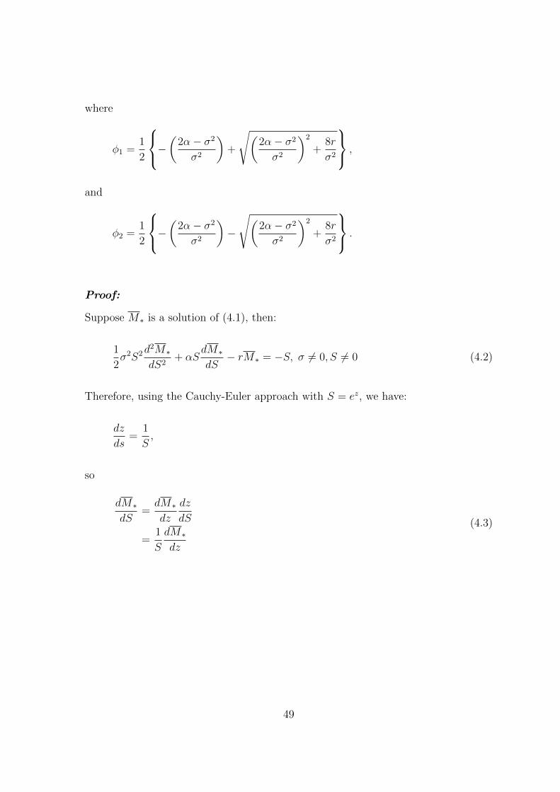
where

φ1 =1

2

−(

2α− σ2

σ2

)+

√(2α− σ2

σ2

)2

+8r

σ2

,

and

φ2 =1

2

−(

2α− σ2

σ2

)−

√(2α− σ2

σ2

)2

+8r

σ2

.

Proof:

Suppose M∗ is a solution of (4.1), then:

1

2σ2S2d

2M∗

dS2+ αS

dM∗

dS− rM∗ = −S, σ 6= 0, S 6= 0 (4.2)

Therefore, using the Cauchy-Euler approach with S = ez, we have:

dz

ds=

1

S,

so

dM∗

dS=dM∗

dz

dz

dS

=1

S

dM∗

dz

(4.3)

49

and

d2M∗

dS2=

d

dS

(dM∗

dS

)=

d

dS

(1

S

dM∗

dz

)= − 1

S2

dM∗

dz+

1

S

d

dS

(dM∗

dz

)= − 1

S2

dM∗

dz+

1

S

d

dz

(dM∗

dz

)(dz

dS

)= − 1

S2

dM∗

dz+

1

S2

d2M∗

dz2

=1

S2

(d2M∗

dz2− dM∗

dz

).

(4.4)

Therefore, (4.3) and (4.4) are substituted in (4.2) as follows:

1

2σ2S2

(1

S2

(d2M∗

dz2− 1

S2

dM∗

dz

))+αS

(1

S

dM∗

dz

)−rM∗ = −ez, σ 6= 0, S 6= 0. (4.5)

That implies:

σ2

2

d2M∗

dz2+

(α− σ2

2

)dM∗

dz− rM∗ = −ez, σ 6= 0. (4.6)

Equation (4.6) is a nonhomogeneous second order linear ODE with constant coef-

ficients. Thus, for the complementary solution, M∗C , the characteristic equation

(associated to the homogeneous part of (4.6) ) is given as:

σ2

2φ2 +

(α− σ2

2

)φ− r = 0 (4.7)

where φ is any function that satisfies (4.7), a∗ = σ2

2, b∗ =

(α− σ2

2

), and c∗ = −r,

50

such that:

φ =−b∗ ±

√b2∗ − 4a∗c∗

2a∗(4.8)

Therefore, the solution of (4.7) is expressed as:

φ1 =1

2

−(

2α− σ2

σ2

)+

√(2α− σ2

σ2

)2

+8r

σ2

,

φ2 =1

2

−(

2α− σ2

σ2

)−

√(2α− σ2

σ2

)2

+8r

σ2

.

(4.9)

So,

M∗C(z) = Aeφ1z +Beφ2z. (4.10)

The nonhomogeneous term in (4.6) is h(z) = −ez , hence, the assumed candidate for

the particular solution is M∗p(z) = Cez

... M ′∗p(z) = Cez = M ′′∗p(z). (4.11)

So (4.8) is substituted in (4.3) as follows:

σ2

2

d2M∗p

dz2+

(α− σ2

2

)dM∗p

dz− rM∗p = −ez. (4.12)

That is:

σ2

2(cez) +

(α− σ2

2

)(cez)− r (cez) = −ez. (4.13)

51

Showing that:

((α− r) c+ 1) ez = 0. (4.14)

So,

c =1

r − α. (4.15)

Hence,

M∗p = cez

=ez

r − α.

(4.16)

Thus,

M∗(z) = Aeφ1z +Beφ2z +ez

r − α. (4.17)

So, replacing ez with S in (4.17) yields (4.18) below:

M(S) = ASφ1 +BSφ2 +S

r − α(4.18)

for

M (1) = 0, M ′ (1) = 1, and r − α =1

2(4.19)

where

A =2φ2 − 1

φ1 − φ2

, φ1 6= φ2 (4.20)

52

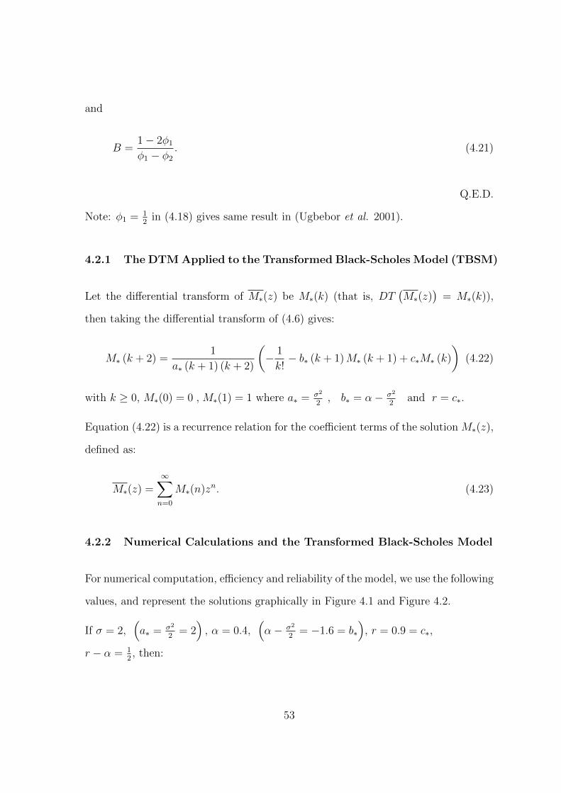
and

B =1− 2φ1

φ1 − φ2

. (4.21)

Q.E.D.

Note: φ1 = 12

in (4.18) gives same result in (Ugbebor et al. 2001).

4.2.1 The DTM Applied to the Transformed Black-Scholes Model (TBSM)

Let the differential transform of M∗(z) be M∗(k) (that is, DT(M∗(z)

)= M∗(k)),

then taking the differential transform of (4.6) gives:

M∗ (k + 2) =1

a∗ (k + 1) (k + 2)

(− 1

k!− b∗ (k + 1)M∗ (k + 1) + c∗M∗ (k)

)(4.22)

with k ≥ 0, M∗(0) = 0 , M∗(1) = 1 where a∗ = σ2

2, b∗ = α− σ2

2and r = c∗.

Equation (4.22) is a recurrence relation for the coefficient terms of the solution M∗(z),

defined as:

M∗(z) =∞∑n=0

M∗(n)zn. (4.23)

4.2.2 Numerical Calculations and the Transformed Black-Scholes Model

For numerical computation, efficiency and reliability of the model, we use the following

values, and represent the solutions graphically in Figure 4.1 and Figure 4.2.

If σ = 2,(a∗ = σ2

2= 2), α = 0.4,

(α− σ2

2= −1.6 = b∗

), r = 0.9 = c∗,

r − α = 12, then:

53

Case I: (The proposed theoretical solution)

From (4.9) and (4.18) we have that:

φ1 = 1.181024968 , φ2 = −0.3810249676, A = −1.128036879 , B = −0.8719631201

and

MP

∗ (z) = −1.128036879e1.181024968z − 0.8719631201e−0.3810249676z + 2z. (4.24)

Case II: (The Exact solution)

MEXACT

∗ (z) = 2ez+

(−√

61

61− 1

)e

110(4+

√61)z+

(−1 +

√61

61

)e−110 (−4+

√61)z. (4.25)

Case III: (The DTM solution with reference to (4.23))

MDTM

∗ (z) = z+3z2

20+

19z3

600− 71z4

8000− 5849z5

1200000− 32107z6

12000000− 2304341z7

5040000000+· · · . (4.26)

Remark 4.2.2: Equations (4.24), (4.25), and (4.26) represent the proposed, exact,

and DTM solutions respectively.

Note: In Figure 4.1, the solid red, long dash green, and dot yellow lines are for the

proposed, DTM, and exact solutions respectively. From graph above, the relationship

between the solutions show that the proposed method is very effective and efficient

when compared with the exact, and the DTM method solutions.

54

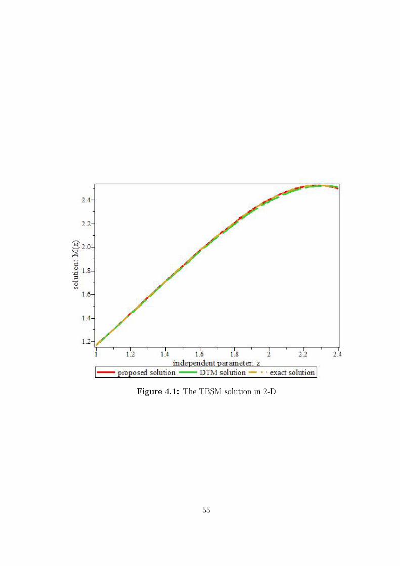
Figure 4.1: The TBSM solution in 2-D

55

4.3 The Generalised Black-Scholes Model via the CEV Stochastic Dy-

namics

In this section, the classical Black-Scholes option pricing model is re-visited. A gener-

alised version of the Black-Scholes model via the application of the constant elasticity

of variance model (CEVM) with or without dividend yield parameter is presented.

4.3.1 Constant Elasticity of Variance Option Pricing Model: A Case of

no Dividend Yield

In what follows, the Black-Scholes model is generalised using the SDE associated with

the CEV model in (2.5).

Proposition 4.3.1:

Associated to the CEV stochastic dynamics in (2.5) is a generalised version of the

Black-Scholes model:

∂Ξ

∂t+ rS

∂Ξ

∂S+

1

2σ2Sξ

∂2Ξ

∂S2− rΞ = 0

where Ξ = Ξ (S, t) is the option value at no dividend yield, S = St is a corresponding

stock price process at time t.

Proof:

Suppose the stock price, St at time t, satisfies the SDE in (2.5), with all parameters

as earlier defined, and that the value of the contingent claim Λ = Λ (S, t) is such that

56

Λ ∈ C2,1 (R× [0, T ]), therefore by Ito lemma, we have:

dΛ =∂Λ

∂tdt+

∂Λ

∂SdS +

1

2

∂2Λ

∂S2〈dS〉

=∂Λ

∂tdt+

∂Λ

∂S

(Stµdt+ σS

ξ2t dWt

)+

1

2

∂2Λ

∂S2

⟨Stµdt+ σS

ξ2t dWt

⟩.

(4.27)

But for:

⟨Stµdt+ σS

ξ2t dWt

⟩=

(Stµdt+ σS

ξ2t dWt

)2

= (Stµdt)2 + 2 (Stµdt)

(σS

ξ2t d (Wt)

)+

(σS

ξ2t d (Wt)

)2

= (Stµ)2 (dt)2 + 2

(StµσS

ξ2t

)(dt) (d (Wt)) + σ2Sξt (d (Wt))

2

= 0 + 0 + σ2Sξt dt

= σ2Sξt dt.

(4.28)

Since (dt)2 = (dt) (dWt) = 0, and (dWt)2 = dt, using the Ito multiplicative table in

Definition 3.3.1. Therefore, (4.27) is expressed as:

dΛ =

(∂Λ

∂t+ µS

∂Λ

∂S+

1

2σ2Sξ

∂2Λ

∂S2

)dt+ σS

ξ2∂Λ

∂SdW. (4.29)

Let Φ(t) be a delta-hedged-portfolio by longing a contingent, and shorting a delta

unit of the underlying asset such that:

Φ(t) = Λ(S, t)−∆S, dΦ(t) = dΛ(s, t)−∆dS, ∆ =∂Λ

∂Sand dΦ(t) = rΦ(t)dt (4.30)

57

in order to make the value of the portfolio riskless, where r is a riskless rate, say bank

account.

Therefore,

dΦ(t) =

(∂Λ

∂t+ µS

∂Λ

∂S+

1

2σ2Sξ

∂2Λ

∂S2

)dt+σS

ξ2∂Λ

∂SdW−∆

(µSdt+ σS

ξ2dW

). (4.31)

That implies that:

dΦ

dt=

(∂Λ

∂t+ µS

∂Λ

∂S+

1

2σ2Sξ

∂2Λ

∂S2

)+ σS

ξ2∂Λ

∂S

dW

dt− ∂Λ

∂S

(µS + σS

ξ2dW

dt

).

Showing that:

dΦ

dt=∂Λ

∂t+

1

2σ2Sξ

∂2Λ

∂S2≡ rΦ. (4.32)

Thus, using (4.30) in (4.32) gives:

∂Λ

∂t+ rS

∂Λ

∂S+

1

2σ2Sξ

∂2Λ

∂S2− rΛ = 0. (4.33)

Thus, the proof is complete for Λ (S, t) = Ξ (S, t) Q.E.D.

Equation (4.33) is referred to as the generalised Black-Scholes model via CEV (CEV-

BSM) on a no-dividend yield basis.

4.3.1.1 Comparison of the Models: The Black-Scholes Model and the

CEV-Black-Scholes Model

In this subsection, the basic features of the two models presented in (2.3) and (4.33)

are compared using their respective SDEs.

Corollary 4.3.1

Suppose ΛoBSM denotes the volatility of the BSM, Λo

CEVM the volatility of the CEV

58

model, ΛrBSM the variance of the BSM, and Λr

CEVM the variance of the CEV model.

Then:

ΛoBSM = σ, Λo

CEVM = σSξ2−1, Λr

BSM = σ2, & ΛrCEVM = σ2Sξ−2. (4.34)

Proof: For St 6= 0, the SDEs associated to the BSM and CEVM as contained in (2.2)

and (2.5) respectively can be expressed as:

dStSt

= µ+ σdWt,

and

dStSt

= µdt+ σSξ2−1

t dWt.

Recall from Ito theorem that the volatility of a one-dimensional SDE of the form:

dX

X= ϕ1dτ + ϕ2dB (τ) , X = X (τ) 6= 0

is defined and denoted as V 0X = ϕ2, where B (τ) is a standard Brownian motion.

Therefore,ΛoBSM = σ,

ΛoCEVM = σS

ξ2−1.

59

But variance by definition, implies the square of the volatility, hence:ΛrBSM = σ2,

ΛrCEVM = σ2Sξ−2.

This completes the proof.

Remark 4.3.1

It is obvious that ΛoCEVM = h (σ, St) is not a constant function but a function of the

underlying asset price St .

4.3.1.2 A Note on Elasticity and Elasticity Parameter

For the computation of elasticity, the following relationship is used (Hsu et al. 2008):

e =

(dΛr

CEVM

dS

)÷(

ΛrCEVM

S

). (4.35)

Therefore, from (4.34), the following is obtained:

dΛrCEVM

dS= (ξ − 2)σ2Sξ−3 and

ΛrCEVM

S= σ2Sξ−3, (4.36)

Therefore,

e = ξ − 2. (4.37)

60

Note: It is obvious from (4.36) with little algebra that for any positive constant c

such that cσ2 = 1 , the following is obtained:

Set = cΛrCEVM . (4.38)

It has been shown empirically that the relationship between the stock price and the

volatility of its return is negative (Hsu et al. 2008). This is guaranteed when ξ < 2 is

considered.

The above result shows that the stock price volatility is a function of the underlying

asset price, not a constant. The next case to be considered is that of dividend yield

inclusion.

4.3.2 The CEV - Black-Scholes Model on a Basis of Dividend Yield

In this subsection, we consider a pricing model for stock option valuation via the ap-

plication of the constant elasticity of variance (CEV) model with dividend yield. This

incorporates into the Black-Scholes model a non-constant volatility power function of

the underlying stock price, and a dividend yield parameter.

Thus, the same approach as in subsection 4.3.1 followed but with the inclusion of

dividend yield parameter in the SDE in (2.3). Recall that Cox and Ross (1976)

considered the CEV diffusion process governed by the SDE in (4.39) below when

q = 0:

dSt = St (µ− q) dt+ σSξ2t d (Wt) (4.39)

where St = S∗ is the solution of (4.39) at time t, ξ represents the rate of elasticity,

q denoting a dividend yield parameter, µ, σ, and Wt = W remain as defined in the

61

earlier section.

In what follows, the Black-Scholes model will be generalised using the SDE associated

with the CEV model in (4.39).

4.3.2.1 The Generalised CEV-Black-Scholes Model on the Basis of Divi-

dend Yield Parameter

Let S∗ be the stock price at time t, satisfying (4.52), such that the value of the

contingent claim is Λd = Λd(S, t) with Λd ∈ C2,1 (R× [0, T ]), so by applying Ito’s

lemma, we have:

dΛd =∂Λd

∂tdt+

∂Λd

∂S∗dS∗ +

1

2

∂2Λd

∂S2∗〈dS∗〉

=∂Λd

∂tdt+

∂Λd

∂S∗

(S∗ (µ− q) dt+ σS

ξ2∗ d (W )

)+

1

2

∂2Λd

∂S2∗

⟨S∗ (µ− q) dt+ σS

ξ2∗ d (W )

⟩.

(4.40)

But:

⟨S∗ (µ− q) dt+ σS

ξ2∗ dWt

⟩=

(S∗ (µ− q) dt+ σS

ξ2∗ dWt

)2

= (S∗ (µ− q) dt)2 + 2 (S∗ (µ− q) dt)(σS

ξ2∗ dWt

)+

(σS

ξ2∗ dWt

)2

= (S∗ (µ− q))2 (dt)2 + 2

(S∗ (µ− q)σS

ξ2∗

)(dt) (dWt)

+ σ2Sξ∗ (dWt)2

= 0 + 0 + σ2Sξ∗dt

= σ2Sξ∗dt

(4.41)

62

where

(Θ)(dWt) =

dt, for Θ = dWt

0, otherwise.(4.42)

Hence, (4.40) becomes:

dΛd =∂Λd

∂tdt+

∂Λd

∂S∗

(S∗ (µ− q) dt+ σS

ξ2∗ d (W )

)+

1

2

∂2Λd

∂S2∗

(σ2Sξ∗dt

). (4.43)

Therefore,

dΛd =

(∂Λd

∂t+ (µ− q)S∗

∂Λd

∂S∗+

1

2σ2Sξ∗

∂2Λd

∂S2∗

)dt+ σS

ξ2∗∂Λd

∂S∗dW. (4.44)

Suppose Ξ(t) is a delta-hedge-portfolio constructed by longing a contingent claim,

and shorting a delta unit of the concerned underlying asset such that:

Ξ(t) = −∆S∗ + Λd(S∗, t), dΞ(t) = dΛd(S∗, t)−∆dS∗,

∆ =∂Λd

∂S∗, and dΞ(t) = rΞ(t)dt.

(4.45)

In a bid to making the portfolio value riskless (say bank account) where r is a riskless

rate, the following is obtained:

dΞ(t) = dΛd(S∗, t)−∆dS∗.

This implies that:

dΞ(t) =

(∂Λd

∂t+ (µ− q)S∗

∂Λd

∂S∗+

1

2σ2Sξ∗

∂2Λd

∂S2∗

)dt

+ σSξ2∗∂Λd

∂S∗dW −∆

((µ− q)S∗dt+ σS

ξ2∗ dW

).

(4.46)

63

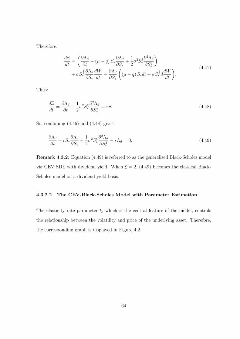
Therefore:

dΞ

dt=

(∂Λd

∂t+ (µ− q)S∗

∂Λd

∂S∗+

1

2σ2Sξ∗

∂2Λd

∂S2∗

)+ σS

ξ2∗∂Λd

∂S∗

dW

dt− ∂Λd

∂S∗

((µ− q)S∗dt+ σS

ξ2∗ ddW

dt

).

(4.47)

Thus:

dΞ

dt=∂Λd

∂t+

1

2σ2Sξ∗

∂2Λd

∂S2∗≡ rΞ (4.48)

So, combining (4.46) and (4.48) gives:

∂Λd

∂t+ rS∗

∂Λd

∂S∗+

1

2σ2Sξ∗

∂2Λd

∂S2∗− rΛd = 0. (4.49)

Remark 4.3.2: Equation (4.49) is referred to as the generalised Black-Scholes model

via CEV SDE with dividend yield. When ξ = 2, (4.49) becomes the classical Black-

Scholes model on a dividend yield basis.

4.3.2.2 The CEV-Black-Scholes Model with Parameter Estimation

The elasticity rate parameter ξ, which is the central feature of the model, controls

the relationship between the volatility and price of the underlying asset. Therefore,

the corresponding graph is displayed in Figure 4.2.

64

Figure 4.2: Estimates of the CEVM distribution

65

Figure 4.2 shows the estimates of the CEVM distribution at maturity time, h(ξ) =

(S (T )− 1, 0)+ using different values of the elasticity parameter for results interpre-

tation, and to show the economic implications of the elasticity rate. For the pur-

pose of simulation, we consider the following values for the concerned parameters:

T = 2.0, σ = 0.3, µ = 0.05 and for ξ = 0.1, ξ = 2, and ξ = 2.5 with red, black, and

green dash lines respectively (with reference to section 4.3.1).

Remark 4.3.3

(a) Elasticity is said to be zero if ξ = 2; therefore, the stock price is lognormally

distributed as indicated in the classical Black-Scholes model.

(b) Elasticity is −1 as proposed by Cox and Ross (1976) if ξ = 1.

(c) When ξ < 2, the so-called leverage effect observed mainly in equity market,

shows that the stock volatility increases as the corresponding price falls.

(d) On the other hand, when ξ > 2, the so-called leverage effect observed mainly in

commodity market, indicates that the volatility of the commodity increases as

the corresponding price increases.

It is remarked here, that in the generalised versions of the Black-Scholes pricing model;

a non-constant volatility power function is introduced, and comparison between the

CEV models with or without dividend yield is made.

4.4 Analytical Solution of the Black-Scholes Model for European Option

Valuation

In this section, analytical solutions of the classical Black-Scholes pricing model for

European options are considered via the application of the PDTM, and the Revised

66

Homotopy Perturbation Method (He’s polynomial technique). The cases considered

include both the integer and the fractional time-order type.

4.4.1 The MDTM Applied for Analytical Solution of Black-Scholes Pric-

ing Model for European Option Valuation

In this subsection, the MDTM is applied to some examples of the classical Black-

Scholes equations (Allahviranloo and Behzadi, 2013; Qiu and Lorenz, 2009; Elbeleze

et al. 2013) as follows:

Example 4.4.1.1 : Consider the following Black-Scholes equation (Allahviranloo

and Behzadi, 2013):

∂v

∂t− ∂2v

∂x2+ (1− k)

∂v

∂x= kv (4.50)

subject to:

v (x, 0) = max (ex − 1, 0) (4.51)

where v is the value of the contingent claim, x = lnS (t), k ∈ N. For simplicity, the

following are re-written as applied in Example 4.4.1:

∂v

∂t= vt,

∂2v

∂x2= vxx,

∂v

∂x= vx.

Suppose the projected differential transform of v () is V (, h+ 1), then taking the

PDT of (4.50) and (4.51) gives:

V (x, h+ 1) =1

h+ 1[V xx (x, h) + (k − 1)V x (x, h)− kV (x, h)] (4.52)

67

and

V (x, 0) = max (ex − 1, 0) . (4.53)

respectively.

This implies that:

V x (x, 0) = V xx (x, 0)

= max (ex, 0)

= ex.

(4.54)

Thus, when h = 0, the following is obtained:

V (x, 1) = V xx (x, 0) + (k − 1)V x (x, 0)− kV (x, 0)

= max (ex, 0) + (k − 1) max (ex, 0)−K max (ex − 1, 0)

= k max (ex, 0)−max (ex − 1, 0)

(4.55)

whence,

V x (x, 1) = V xx (x, 1) = 0. (4.56)

So for h = 1,

V (x, 2) =1

2(V xx (x, 1) + (k − 1)V x (x, 1)− kV (x, 1))

=−k2

2(max (ex, 0)−max (ex − 1, 0)).

(4.57)

Similarly, from (4.57), the following is obtained:

V x (x, 2) = 0 = V xx (x, 2) . (4.58)

68

When h = 2,

V (x, 3) =1

3(V xx (x, 2) + (k − 1)V x (x, 2))

=k3

6(max (ex, 0)−max (ex − 1, 0)).

(4.59)

Hence,

v (x, t) = V (x, 0) +∞∑h=1

V (x, h) th

= max (ex − 1, 0) + (kt) Z− (kt)2

2!Z +

(kt)3

3!Z (x) + · · ·

(4.60)

where

Z (x) = max (ex, 0)−max (ex − 1, 0) . (4.61)

Therefore:

v (x, t) = max (ex − 1, 0)

+∞∑h=1

(−1)h+1 (kt)h

h!max (ex, 0)−max (ex − 1, 0).

(4.62)

Equation (4.62) is the exact solution of (4.50).

Example 4.4.1.2: Consider the following Black-Scholes equation ((Qiu and Lorenz,

2009; Elbeleze et al. 2013), Example 7 & Example 2 respectively, for α = 1):

∂v

∂t+ 0.08 (2 + Sinx)2 x2 ∂

2v

∂x2+ 0.06x

∂v

∂x= 0.06v (4.63)

subject to:

v (x, 0)−max(x− 25e−0.06, 0

)= 0. (4.64)

69

Following the same approach in Example 4.4.1.1 by taking the PDT of (4.63) and

(4.64) gives:

(h+ 1)V (x, h+ 1) =(−0.08 (2 + Sinx)2 x2V xx (x, h)

)+ (−0.06xV x (x, h) + 0.06V (x, h))

(4.65)

subject to:

V (x, 0) = max(x− 25e−0.06, 0

). (4.66)

This implies that:

V x (x, 0) = 1, and V xx (x, 0) = 0. (4.67)

So, when h = 0,

V (x, 1) =(−0.06x+ 0.06 max(x− 25e−0.06, 0)

)= −0.06

(x−max(x− 25e−0.06, 0)

) (4.68)

and

V x (x, 1) = 0 = V xx (x, 1) . (4.69)

So when h = 1 ,

V (x, 2) =1

2(0.06V (x, 1))

=−(0.06)2

2

(x−max(x− 25e−0.06, 0)

).

(4.70)

As such,

V x (x, 2) = 0 = V xx (x, 2) . (4.71)

70

So when h = 2 ,

V (x, 3) =1

3(0.06V (x, 2))

=−(0.06)3

3

(x−max(x− 25e−0.06, 0)

).

(4.72)

Hence,

v (x, t) =∞∑h=0

V (x, h)th = V (x, 0) + V (x, 1)t+ V (x, 2)t2 + V (x, 3)t3 + · · ·

= max(x− 25e−0.06, 0) +

(−0.06t− (0.06t)2

2!− (0.06t)3

3!+ · · ·

)U (x)

where

U (x) =(x−max(x− 25e−0.06, 0)

). (4.73)

Therefore:

v (x, t) = max(x− 25e−0.06, 0

)−(

0.06t+(0.06t)2

2!+

(0.06t)3

3!+ · · ·

)U (x)

= max(x− 25e−0.06, 0

)− U (x)

∞∑n=1

(0.06t)n

n!.

(4.74)

So, simplifying (4.74) using (4.73) yields:

v(x, t) = max(x− 25e−0.06, 0

)+(1− e0.06t

) (x−max

(x− 25e−0.06, 0

))= x

(1− e0.06t

)+ max

(x− 25e−0.06, 0

)e0.06t.

(4.75)

Equation (4.75) is the exact solution of (4.63) subject to (4.64).

Figure 4.4 is the 3D plot of the exact solution to the problem in example 4.4.1.2

while Figure 4.3 is the 3D plot of the approximate solution to example 4.4.1.2.

71

Figure 4.3: The approximate solution for problem example 4.4.1.2

72

Figure 4.4: The exact solution for problem example 4.4.1.2

73

Remark 4.4.1.2

The MDTM has been successfully applied to Black-Scholes Equation for European

Option Valuation. Some illustrative and numerical examples were solved to test the

efficiency of the proposed method. The results obtained converge faster to their exact

forms, even with less computation, without linearization or perturbation; showing that

the method can also be used easily for approximate solutions in a direct form. These

easily computed results represent the analytical values of the associated European

call options, the same algorithm can be followed for European put options.

4.4.2 He’s Polynomials Applied to the Black-Scholes Pricing Model for

Stock Option Valuation

In this subsection, we apply the He’s polynomials for solving the classical Black-

Scholes pricing model with stock as the underlying asset. Our goal here, is therefore, to

provide analytical solutions to the Black–Scholes option pricing model for a particular

form of (4.46) using the He’s polynomials method as an alternative method, to be

used for results comparison.

4.4.2.1 The Pricing Model and the He’s Polynomial

Here, the He’s Polynomials approach is applied to the model equation as follows,

where w = w (x, t) represents the value of the contingent claim, and x = ln S

(t)(Allahviranloo and Behzadi, 2013).

Problem 4.4.2.1.1: Consider the following Black-Scholes equation:

∂w

∂t+ x2∂

2w

∂x2+

1

2x∂w

∂x= w (4.76)

74

subject to:

w (x, 0) = max(x3, 0

)=

x3, for x > 0,

0, for x ≤ 0.(4.77)

Suppose in an integral form, where I t0 (·) =∫ t

0(·) dt and (4.76) is re-written as (4.78),

then (4.78) is reformulated as (4.79) below:

∂w

∂t= −

(x2∂

2w

∂x2+

1

2x∂w

∂x− w

)(4.78)

and

w (x, t) = max(x3, 0

)− pI t0

(x2∂

2w

∂x2+

1

2x∂w

∂x− w

). (4.79)

Applying the convex homotopy method to (4.79) gives:

∞∑n=0

pnwn = max(x3, 0

)−pI t0

(x2

∞∑n=0

pn∂2wn∂x2

+1

2x∞∑n=0

pn∂wn∂x−∞∑n=0

pnwn

)(4.80)

This implies that:

w0 + pw1 + p2w2 + · · · = max(x3, 0

)+

− pI t0x2

(∂2w0

∂x2+ p

∂2w1

∂x2+ p2∂

2w2

∂x2+ · · ·

)+x

2

(∂w0

∂x+ p

∂w1

∂x+ p2∂w2

∂x+ · · ·

)−(w0 + pw1 + p2w2 + · · ·

).

(4.81)

So comparing the coefficients of the equal powers of p gives the following:

p(0) : w0 = max(x3, 0

),

75

p(1) : w1 = −I t0(x2∂

2w0

∂x2+x

2

∂w0

∂x− w0

),

p(2) : w2 = −I t0(x2∂

2w1

∂x2+x

2

∂w1

∂x− w1

),

p(3) : w3 = −I t0(x2∂

2w2

∂x2+x

2

∂w2

∂x− w2

),

...

p(k) : w3 = −I t0(x2∂

2wk−1

∂x2+x

2

∂wk−1

∂x− wk−1

).

Thus, simplifying p(1), p(2), p(3) and so on with w0 = max (x3, 0) for x ≥ 0 gives:

w0 = x3, w1 = −13

2x3t, w2 =

169

8x3t2, w3 =

−2197

48x3t3,

w4 =28561

384x3t4, w5 =

−371293

3840x3t5, · · · .

Therefore:

w (x, t) = w1 + w2 + w3 + w4 + · · ·

= x3 − 13

2x3t+

169

8x3t2 − 2197

48x3t3 +

28561

384x3t4 − 371293

3840x3t5 + · · ·

= x3

(1 + (−6.5t) +

(−6.5t)2

2!+

(−6.5t)3

3!+

(−6.5t)4

4!+

(−6.5t)5

5!+ · · ·

)∼= x3e−6.5t.

(4.82)

The exact and the He’s polynomial solutions of problem 4.4.2.1.1 are graphically

displayed in Figure 4.5 and Figure 4.6 respectively.

76

Figure 4.5: The exact solution for problem 4.4.2.1.1

77

Figure 4.6: The approximate solution for problem 4.4.2.1.1

78

Note: Figure 4.5 and Figure 4.6 represent the graphs of the exact solution and the

He’s polynomials solution (including terms up to power 5) respectively, to the classical

Black-Scholes model for stock option valuation. These are obtained via the application

of He’s polynomials as the proposed technique. This technique is very much efficient

and reliable as it gives the exact solution of the solved problem in a very simple and

quick manner even with less computational work while still maintaining high level of

accuracy.

4.5 The Time-Fractional Black-Scholes Option Pricing Model on No-

Dividend Paying Equity

To be considered in this section is a generalisation of (2.3) with regard to fractional

order, β ∈ R or C, not necessarily an integer. This generalisation will be referred to

as Time-fractional Black-Scholes Model (TFBSM) of the form:

∂βΞ

∂tβ+ ζ1 (S, t)

∂2Ξ

∂S2+ ζ2 (S, t)

∂Ξ

∂S= rΞ , β ∈ (0, 1] (4.83)

subject to a given initial or boundary condition(s). We donote ζi (·, ·) , i ∈ N, as non-

zero functions, while Ξ represents the fair value of the contingent claim associated

with the time fractional Black-Scholes model.

4.5.1 Illustrative Examples and Applications

In this section, some examples of time-fractional Black-Scholes equations will be solved

with the proposed algorithmic technique: MDTM as follows.

Problem 4.5.1.1: Consider the following time-fractional Black-Scholes equation

79

(problem 4.4.2.1.1 for α = 1 ):

∂αw

∂tα+ x2∂

2w

∂x2+x

2

∂w

∂x− w = 0 , 0 < α ≤ 1 (4.84)

subject to:

w (x, 0) = max(x3, 0

)=

x3, for x > 0,

0, for x ≤ 0.(4.85)

Here, the study will consider x > 0 and take ∂W (x,ξ)∂x

as the projected differential

transform (PDT) of w = w (x, t) as follows: So taking the PDTM of (4.84) and (4.85)

gives:

W (x, 1 + ξ) =Γ (1 + αξ)

Γ (1 + α(1 + ξ))

(−x2∂

2W (x, ξ)

∂x2− 1

2

∂W (x, ξ)

∂x+W (x, ξ)

)(4.86)

subject to:

W (x, 0) = x3. (4.87)

That implies:

∂W (x, 0)

∂x= 3x2 and

∂2W (x, 0)

∂x2= 6x. (4.88)

So, when ξ = 0,

W (x, 1) =Γ (1)

Γ (1 + α)

(−x2∂

2W (x, 0)

∂x2− 1

2

∂W (x, 0)

∂x+W (x, 0)

)

showing that:

W (x, 1) =Γ (1)

Γ (1 + α)

(−6x3 − 3

2x3 + x3

)=

(−6.5x3)

Γ (1 + α). (4.89)

80

From (4.89), the following is obtained:

∂W (x, 1)

∂x=

(−19.5x2)

Γ (1 + α)&∂2W (x, 1)

∂x2=

(−39x)

Γ (1 + α)(4.90)

Thus, for ξ = 1,

W (x, 2) =Γ (1 + α)

Γ (1 + 2α)

(−x2∂

2W (x, 1)

∂x2− 1

2

∂W (x, 1)

∂x+W (x, 1)

)=

Γ (1 + α)

Γ (1 + 2α)

(39x3 + 9.75x3 − 6.5x3

Γ (1 + α)

)=

(6.5)2 x3

Γ (1 + 2α).

(4.91)

So (4.91) gives:

∂W (x, 2)

∂x=

(126.75x2)

Γ (1 + 2α)&∂2W (x, 2)

∂x2=

(253.5x)

Γ (1 + 2α)(4.92)

so when ξ = 2 ,

W (x, 3) =Γ (1 + 2α)

Γ (1 + 3α)

(−x2∂

2W (x, 2)

∂x2− 1

2

∂W (x, 2)

∂x+W (x, 2)

)=

Γ (1 + 2α)

Γ (1 + 3α)

(−253.5x3 − 63.375x3 + 42.25x3

Γ (1 + 2α)

)=

(−6.5)3 x3

Γ (1 + 3α).

(4.93)

Similarly, the recurrence relation below is obtained:

W (x, h) =(−6.5)hx3

Γ (1 + hα), h ∈ Z+. (4.94)

81

Hence,

w (x, t) =∞∑η=0

W (x, η) tαη

= W (x, 0) +W (x, 1) tα +W (x, 2) t2α +W (x, 3) t3α + · · ·

= x3 − (6.5tα)x3

Γ (1 + α)+

(6.5)2 x3t2α

Γ (1 + 2α)− (6.5)3 x3t3α

Γ (1 + 3α)+ · · ·

=

(1 +

(−6.5tα)

Γ (1 + α)+

(−6.5tα)2

Γ (1 + 2α)+

(−6.5tα)3

Γ (1 + 3α)+ · · ·

)x3

= x3

∞∑n=0

(−6.5tα)n

Γ (1 + nα)

= x3Eα (−6.5tα) .

(4.95)

It is therefore remarked that w (x, t) = x3 exp (−6.5t) is the exact solution of problem

4.5.1.1 when α = 1 (a special case).

Problem 4.5.1.2: Consider the following time-fractional Black-Scholes equation

(with reference to example 4.4.1.1, and Hariharan et al., 2013) for α = 1.

∂αw

∂tα=∂2w

∂x2+ (k − 1)

∂w

∂x+ kw, w = w(x, t), 0 < α ≤ 1 (4.96)

subject to:

w (x, 0) = max (ex − 1, 0) . (4.97)

By method of solution, taking the MDTM of (4.96) and (4.97) gives:

W (x, ξ + 1) =Γ (1 + αξ)

Γ (1 + α(1 + ξ))

(∂2W (x, ξ)

∂x2+ (k − 1)

∂W (x, ξ)

∂x− kW (x, ξ)

)(4.98)

82

and

W (0, ξ) = max (ex − 1, 0) . (4.99)

respectively. So,

∂W (0, ξ)

∂x=∂2W (0, ξ)

∂x2= max (ex, 0) . (4.100)

Thus, when ξ = 0, we have:

W (x, 1) =Γ (1)

Γ (1 + α)

(∂2W (x, 0)

∂x2+ (k − 1)

∂W (x, 0)

∂x− kW (x, 0)

)=

1

Γ (1 + α)max (ex, 0) + (k − 1) max (ex, 0)−K max (ex − 1, 0) .

That implies:

W (x, 1) =1

Γ (1 + α)k (max (ex, 0)−max (ex − 1, 0)) . (4.101)

From (4.101),

∂W (x, 1)

∂x=∂2W (x, 1)

∂x2= 0. (4.102)

When ξ = 1,

W (x, 2) =−kΓ (1 + α)

Γ (1 + 2α)(W (x, 1))

=Γ (1 + α)

Γ (1 + 2α)

[−k

Γ (1 + α)k (max (ex, 0)−max (ex − 1, 0))

]=

−k2

Γ (1 + 2α)max (ex, 0)−max (ex − 1, 0) .

(4.103)

83

From (4.103),

∂W (x, 2)

∂x= 0 =

∂2W (x, 2)

∂x2(4.104)

so, when ξ = 2,

W (x, 3) =−kΓ (1 + 2α)

Γ (1 + 3α)(W (x, 2))

=Γ (1 + 2α)

Γ (1 + 3α)

[−k

Γ (1 + 2α)

(−k2) (max (ex, 0)−max (ex − 1, 0))

]=

k3

Γ (1 + 3α)max (ex, 0)−max (ex − 1, 0) .

(4.105)

From (4.105),

∂W (x, 3)

∂x= 0 =

∂2W (x, 3)

∂x2(4.106)

so, when ξ = 3,

W (x, 4) =Γ (1 + 3α)

Γ (1 + 4α)(−kW (x, 3))

=−k4

Γ (1 + 4α)(max (ex, 0)−max (ex − 1, 0)) .

(4.107)

Suppose the following is set:

B∗ (x) = (max (ex, 0)−max (ex − 1, 0)) (4.108)

84

then,

w (x, t) =∞∑η=0

W (x, η) tαη

= Wx,0 +Wx,1tα +Wx,2t

2α +Wx,3t3α + · · ·

= max (ex − 1, 0)

+B∗ (x)

(ktα)

Γ (1 + α)− (ktα)2

Γ (1 + 2α)+

(ktα)3

Γ (1 + 3α)− (ktα)4

Γ (1 + 4α)+ · · ·

= max (ex − 1, 0) +B∗ (x)

∞∑n=1

(−1)n+1 (ktα)n

Γ (1 + nα)

= max (ex − 1, 0)−B∗ (x)∞∑n=1

(−ktα)n

Γ (1 + nα)

= max (ex − 1, 0)− max (ex, 0)−max (ex − 1, 0) −1 + Eα(−ktα)

= max (ex − 1, 0)Eα(−ktα) + max (ex, 0) (1− Eα(−ktα))

(4.109)

where Eα(−ktα) denotes a one-parameter Mittag-Leffler function.

It is remarked that a special case of Problem 4.5.1.2 at α = 1 has an exact solution:

w (x, t) = max (ex − 1, 0)

+∞∑n=1

(−1)n+1 (kt)n

n!max (ex, 0)−max (ex − 1, 0)

= max (ex − 1, 0) e−kt + max (ex, 0)(1− e−kt

).

(4.110)

Problem 4.5.1.3: Consider the following fractional Black-Scholes equation (Ref.

example 4.4.1.2, and Kumar et al. 2014 for α = 1):

∂αw

∂tα+ 0.08 (2 + Sinx)2 x2∂

2w

∂x2+ 0.06x

∂w

∂x− 0.06w = 0 (4.111)

85

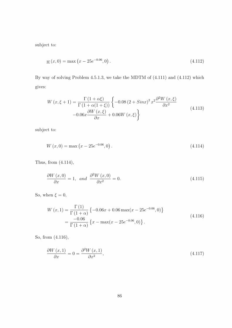
subject to:

w (x, 0) = max(x− 25e−0.06, 0

). (4.112)

By way of solving Problem 4.5.1.3, we take the MDTM of (4.111) and (4.112) which

gives:

W (x, ξ + 1) =Γ (1 + αξ)

Γ (1 + α(1 + ξ))

−0.08 (2 + Sinx)2 x2∂

2W (x, ξ)

∂x2

−0.06x∂W (x, ξ)

∂x+ 0.06W (x, ξ)

(4.113)

subject to:

W (x, 0) = max(x− 25e−0.06, 0

). (4.114)

Thus, from (4.114),

∂W (x, 0)

∂x= 1, and

∂2W (x, 0)

∂x2= 0. (4.115)

So, when ξ = 0,

W (x, 1) =Γ (1)

Γ (1 + α)

−0.06x+ 0.06 max(x− 25e−0.06, 0)

=−0.06

Γ (1 + α)

x−max(x− 25e−0.06, 0)

.

(4.116)

So, from (4.116),

∂W (x, 1)

∂x= 0 =

∂2W (x, 1)

∂x2, (4.117)

86

so for ξ = 1 ,

W (x, 2) =Γ (1 + α)

Γ (1 + 2α)(0.06W (x, 1))

=Γ (1 + α)

Γ (1 + 2α)

[0.06

−0.06

Γ (1 + α)

(x−max(x− 25e−0.06, 0)

)]=−(0.06)2

Γ (1 + 2α)

x−max(x− 25e−0.06, 0)

.

(4.118)

So, from (4.118),

∂W (x, 2)

∂x= 0 =

∂2W (x, 2)

∂x2, (4.119)

so when ξ = 2 ,

W (x, 3) =Γ (1 + 2α)

Γ (1 + 3α)(0.06W (x, 3))

= − (0.06)3

Γ (1 + 3α)

x−max(x− 25e−0.06, 0)

.

(4.120)

Similarly, in recurrent form, the following holds:

W (x, η) = − (0.06)η

Γ (1 + ηα)

x−max(x− 25e−0.06, 0)

, η ∈ N. (4.121)

Set in (4.121) the following:

N∗ (x) =x−max(x− 25e−0.06, 0)

. (4.122)

87

Hence,

w (x, t) =∞∑h=0

W (x, h) tαh

= W (x, 0) +W (x, 1) tα +W (x, 2) t2α +W (x, 3) t3α + · · ·

= max(x− 25e−0.06, 0

)−N∗ (x)

(0.06tα)

Γ (1 + α)+

(0.06tα)2

Γ (1 + 2α)+

(0.06tα)3

Γ (1 + 3α)+ · · ·

= max

(x− 25e−0.06, 0

)−N∗ (x)

∞∑n=1

(0.06tα)n

Γ (1 + nα)

= max(x− 25e−0.06, 0

)−N∗ (x) −1 + Eα(0.06tα) .

(4.123)

Further simplification of (4.123) yields:

w (x, t) = max(x− 25e−0.06, 0

)−(x−max(x− 25e−0.06, 0

)(−1 + Eα(0.06tα))

= x 1− Eα(0.06tα)+ max(x− 25e−0.06, 0

)Eα(0.06tα).

(4.124)

It is remarked that when α = 1, Problem 4.5.1.3 has a special case whose exact

solution is:

w (x, t) = max(x− 25e−0.06, 0

)+ (1− e0.06t)

x−max(x− 25e−0.06, 0)

= x

(1− e0.06t

)+ max

(x− 25e−0.06, 0

)e0.06t.

(4.125)

Note: References are made to Figures 4.7-4.12 for the graphical solutions of problems

4.5.1.1, 4.5.1.2, and 4.5.1.3 in terms of their contingent claim values .

88

Figure 4.7: Contingent Claim Value (CCV) for x ∈ [0, 2] , t ∈ [0, 9]

89

Figure 4.8: Contingent Claim Value (CCV) for x ∈ [0, 2] , t ∈ [0, 18]

90

Figure 4.9: Contingent Claim Value (CCV) for x ∈ [0, 45] , t ∈ [0, 45]

91

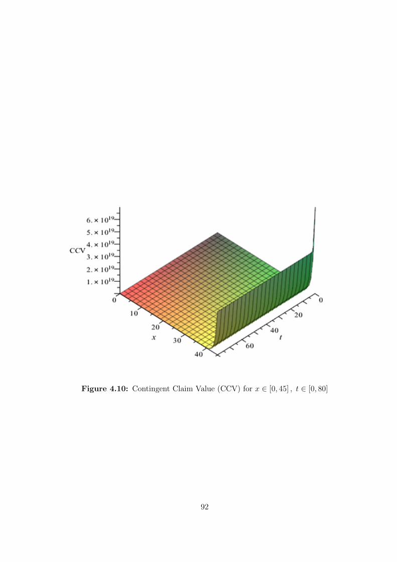
Figure 4.10: Contingent Claim Value (CCV) for x ∈ [0, 45] , t ∈ [0, 80]

92

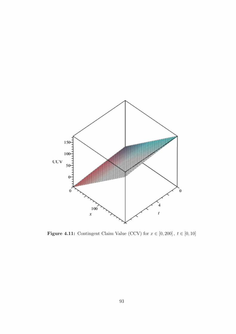
Figure 4.11: Contingent Claim Value (CCV) for x ∈ [0, 200] , t ∈ [0, 10]

93

Figure 4.12: Contingent Claim Value (CCV) for x ∈ [0, 400] , t ∈ [0, 10]

94

Remark 4.5.2

In section 4.5, analytical solutions of the time-fractional Black-Scholes equations for

European call option were obtained via the proposed relatively new approximate-

analytic technique, PDTM. The graphical representation of the solutions were pre-

sented in Figures 4.7-4.12. Figure 4.7 and Figure 4.8 are for problem 4.5.1.1 , Figure

4.9 and Figure 4.10 are for problem 4.5.1.2, while Figure 4.11 and Figure 4.12 are for

problem 4.5.1.3. For each case, same interval is used for x while different intervals for

t.. The application of this method for analytical solutions of time-fractional Black-

Scholes model is new to the best of our knowledge. These present results showed

that the result in subsection 4.4.1 is a special case of this present work for α = 1.

Consequently, it is remarked that the time-fractional Black-Scholes equation for Eu-

ropean option valuation is a generalisation of the classical Black-Scholes equations for

European option valuation at order, α = 1.

4.6 The Generalised Bakstein and Howison Model

In this section, the Bakstein and Howison Model is generalised. This is done by using

the volatility function associated with the transaction-cost of Baskstein and Howison

(2003) in the CEV-BSM in section 4.3. Thereafter, consider the analytical solutions

of this generalised Bakstein and Howison model, and its extended version to time-

fractional order type are considered.

4.6.1 The Generalisation Procedures

This subsection considers a case where the volatility parameter, σ can be expressed as

a function of the following: time, τ , stock price, S, and the differential coefficients of

95

the option price, Φ. In particular, that of non-constant modified volatility function:

σ =_σ

(τ, S,

∂Φ

∂S,∂2Φ

∂S2

)(4.126)

is to be considered. So, the CEV-BSM in (4.46) becomes:

∂Φ

∂τ+ rS

∂Φ

∂S+

1

2Sξ

_σ

2(τ, S,

∂Φ

∂S,∂2Φ

∂S2

)∂2Φ

∂S2− rΦ = 0. (4.127)

Note: Equation (4.46) can be improved using (4.139) from the aspect of transaction

costs inclusion, large trader and illiquid markets effect. In this regard, the approach

of Frey and Patie (2002) and Frey and Stremme (1997) for the effects on the price

with the result is followed:

σ =_σ

(τ, S,

∂Φ

∂S,∂2Φ

∂S2

)(1− ρSλ(S)

∂2Φ

∂S2

)(4.128)

where σ is the traditional volatility, ρ is a constant measuring the liquidity of the

market, and λ is the price of risk.

Following the assumption that the price of risk is unity, a special case where λ (S) = 1

and a little algebra with the notion that:

1 ≈ (1− f∗)2 (1 + 2f∗ + O (f∗)3)

96

where f∗ is a variable function. Thus, (4.128) is written as:

_σ

(τ, S,

∂Φ

∂S,∂2Φ

∂S2

)2

=_σ

2

=

σ

(1− ρS∂

2Φ

∂S2

)−12

= σ2

(1− ρS∂

2Φ

∂S2

)−2

≈ σ2

(1 + 2ρS

∂2Φ

∂S2

).

(4.129)

Therefore (4.127) becomes:

∂Φ

∂τ+ rS

∂Φ

∂S+

1

2Sξ[σ2

(1 + 2ρS

∂2Φ

∂S2

)]∂2Φ

∂S2− rΦ = 0 (4.130)

such that Φ (S, T ) = h (S), S ∈ [0,∞). For the translation, t + τ = T (T is time at

maturity such that τ ∈ [0, T ]) and using w (S, t) = Φ (S, τ), (4.130) becomes:

∂w

∂t+ rS

∂w

∂S+

1

2Sξσ2

(1 + 2ρS

∂2w

∂S2

)∂2w

∂S2− rw = 0, w (S, 0) = h (S) . (4.131)

Note: For ξ = 2, equation (4.131) has an exact solution (Esekon, 2013) of the form:

w (S, t) = S − ρ−1√S0

√S exp

(r + σ2

4

2

)t+

√S0

4exp

(r +

σ2

4

)t

. (4.132)

For σ, S0, S, |ρ| > 0 while r, t ≥ 0, S0 as an initial stock price, with:

w (S, 0) = max

S − ρ−1

(√S0S +

S0

4

), 0

. (4.133)

Remark 4.6.1.1: It is obvious that (4.131) generalises the Bakstein and Howison

(2003) model. Gonzalez-Gaxiola et al. (2015) considered the approximate solution

97

of a particular case of (4.131) via the application of the Adomian Decomposition

Method. Thus, our results will be compared with theirs.

4.6.1.1 The MDTM Applied to the Generalised Nonlinear Model

In this subsection, the MDTM approach is applied to the model equation (4.131) as

follows. Equation (4.131) is re-expressed as:

∂w

∂t= −rS ∂w

∂S− 1

2Sξσ2

(1 + 2ρS

∂2w

∂S2

)∂2w

∂S2+ rw (4.134)

subject to:

w (S, 0) = max

S − ρ−1

(√S0S +

S0

4

), 0

.

For simplicity, (4.134) is re-expressed as follows:

∂w

∂t= −

rS∂w

∂S+

1

2Sξσ2

∂2w

∂S2+ 2ρS

(∂2w

∂S2

)2− rw

. (4.135)

At projection, the transformation of (4.135) using MDTM yields:

(k + 1)Hk+1 (S) = −rSH ′k (S) + rHk (S)

−

1

2Sξσ2

(H ′′k (S) + 2ρS

k∑n=0

H ′′n (S)H ′′k−n (S)

).

(4.136)

Re-writing (4.136) for Hk+1 = Hk+1(S) gives:

Hk+1 =−1

k + 1

rSH ′k +

1

2Sξσ2

(H ′′k + 2ρS

k∑n=0

H ′′nH′′k−n

)− rHk

(4.137)

98

subject to:

H0 = max

S − ρ−1

(√S0S +

S0

4

), 0

. (4.138)

When k = 0,

H1 = −(rSH ′0 +

1

2Sξσ2 (H ′′0 + 2ρSH ′′0H

′′0 )− rH0

). (4.139)

When k = 1,

H2 = −1

2

rSH ′1 +

1

2Sξσ2

(H ′′1 + 2ρS

1∑n=0

H ′′1H′′1−n

)− rH1

=−1

2

(rSH ′1 +

1

2Sξσ2 (H ′′1 + 4ρSH ′′0H

′′1 )− rH1

).

(4.140)

When k = 2,

H3 = −1

3

rSH ′2 +

1

2Sξσ2

(H ′′2 + 2ρS

2∑n=0

H ′′nH′′2−n

)− rH2

=−1

3

(rSH ′2 +

1

2Sξσ2 (H ′′2 + 2ρS (2H ′′0H

′′2 +H ′′1H

′′1 ))− rH1

).

(4.141)

When k = 3,

H4 = −1

4

rSH ′3 +

1

2Sξσ2

(H ′′3 + 2ρS

3∑n=0

H ′′nH′′3−n

)− rH3

=−1

4

(rSH ′3 +

1

2Sξσ2 (H ′′3 + 4ρS (H ′′0H

′′3 + 2H ′′1H

′′2 ))− rH3

).

(4.142)

When k = 4,

H5 = −1

5

rSH ′4 +

1

2Sξσ2

(H ′′4 + 2ρS

4∑n=0

H ′′nH′′4−n

)− rH4

=−1

5

(rSH ′4 +

1

2Sξσ2 (H ′′4 + 2ρS (2H ′′0H

′′4 + 2H ′′1H

′′3 +H ′′2H

′′2 ))− rH4

).

(4.143)

99

In general, for an integer k∗ such that k∗ ∈ [1,∞), the following is obtained:

Hk∗ =−1

k∗

rSH ′k∗−1 +

1

2S2σ2

(H ′′k∗−1 + 2ρS

k∗−1∑n=0

H ′′nH′′k∗−n−1

)− rHk∗−1

. (4.144)

4.6.1.2 Numerical Illustration and Applications

Recall (4.132) and (4.133) as follows:

w (S, t) = w = S−ρ−1√S0

√S exp

(r + σ2

4

2

)t+

√S0

4exp

(r +

σ2

4

)t

(4.145)

and

w (S, 0) = max

S − ρ−1

(√S0S +

S0

4

), 0

. (4.146)

For numerical computation, the following cases will be considered:

Case 4.6.1.2.1 For r = 0, |ρ| = 0.01, ξ = 2, σ = 0.4, S0 = 4, thus the exact

solution and initial condition are:

w (S, t) = S + 200

√S exp

(t

50

)+

1

2exp

(t

100

)(4.147)

and

w (S, 0) = S + 200√S + 100 (4.148)

respectively.

So, applying the PDTM with the parameters in Case 4.6.1.2.1 through (4.137)-

100

(4.1143) gives the following:

H (S, 0) = H0 = S + 200√S + 100, (4.149)

H(S, 1) = H1 = − S25

(−50

S3/2− 50

S2

), (4.150)

H(S, 2) = −S2

25

(− 8

25

(−50

S3/2− 50

S2

)(75

S5/2+

100

S3

)− 4S

25

(75

S5/2+

100

S3

)2

− 4S

25

(−50

S3/2− 50

S2

)(−375

2S7/2+

300

S4

)− S

50

(−50

(−425

(75S5/2 + 100

S3

)2 − 425

( −50S3/2 − 50

S2

) ( −3752S7/2 − 300

S4

)S3/2

)

− 1

S3/2

(50

(− 8

25

(−50

S3/2− 50

S2

)(75

S5/2+

100

S3

)− 4S

25

(75

S5/2+

100

S3

)2

−4S

25

(−50

S3/2− 50

S2

) (−375

2S7/2+

300

S4

)))).

(4.151)

101

Whence,

w (S, t) =∞∑η=0

H (S, η) tη

= H (S, 0) +H (S, 1) t+H (S, 2) t2 +H (S, 3) t3 + · · ·

=(S + 200

√S + 100

)− S

25

(−50

S3/2− 50

S2

)t

+

(−S

2

25

(− 8

25

(−50

S3/2− 50

S2

)(75

S5/2+

100

S3

)− 4S

25

(75

S5/2+

100

S3

)2

− 4S

25

(−50

S3/2− 50

S2

)(−375

2S7/2+

300

S4

)− 1

50√S

(−50

(−4

25

(75

S5/2+

100

S3

)2

− 4

25

(−50

S3/2− 50

S2

)(−375

2S7/2− 300

S4

))

− 1

S3/2

(50

(− 8

25

(−50

S3/2− 50

S2

)(75

S5/2+

100

S3

)− 4S

25

(75

S5/2+

100

S3

)2

−4S

25

(−50

S3/2− 50

S2

) (−375

2S7/2+

300

S4

))))))t2 + · · · .

(4.152)

Figure 4.13 is the graphics for approximate solution for Case 4.6.1.2.1, for S ∈ [0.1, 10]

and t ∈ [0, 1] while Figure 4.14 is the graphics for exact solution for Case 4.6.1.2.1,

for S ∈ [0.1, 10] and t ∈ [0, 1].

102

Figure 4.13: Approximate solution for Case 4.6.1.2.1

103

Figure 4.14: Exact solution for Case 4.6.1.2.1

104

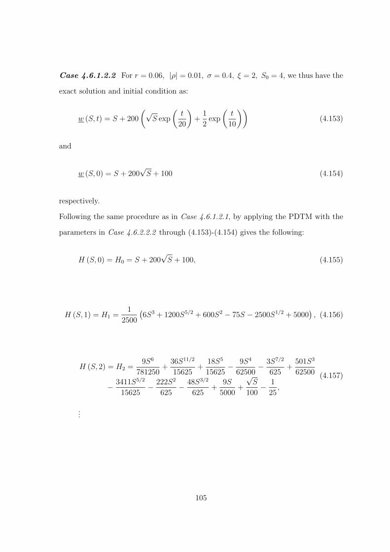
Case 4.6.1.2.2 For r = 0.06, |ρ| = 0.01, σ = 0.4, ξ = 2, S0 = 4, we thus have the

exact solution and initial condition as:

w (S, t) = S + 200

(√S exp

(t

20

)+

1

2exp

(t

10

))(4.153)

and

w (S, 0) = S + 200√S + 100 (4.154)

respectively.

Following the same procedure as in Case 4.6.1.2.1, by applying the PDTM with the

parameters in Case 4.6.2.2.2 through (4.153)-(4.154) gives the following:

H (S, 0) = H0 = S + 200√S + 100, (4.155)

H (S, 1) = H1 =1

2500

(6S3 + 1200S5/2 + 600S2 − 75S − 2500S1/2 + 5000

), (4.156)

H (S, 2) = H2 =9S6

781250+

36S11/2

15625+

18S5

15625− 9S4

62500− 3S7/2

625+

501S3

62500

− 3411S5/2

15625− 222S2

625− 48S3/2

625+

9S

5000+

√S

100− 1

25,

(4.157)

...

105

Whence,

w (S, t) =∞∑η=0

W (S, η) tη

= H (S, 0) +H (S, 1) t+H (S, 2) t2 +H (S, 3) t3 + · · ·

=(S + 200

√S + 100

)+

(1

2500

(6S3 + 1200S5/2 + 600S2 − 75S − 2500S1/2 + 5000

))t

+

(9S6

781250+

36S11/2

15625+

18S5

15625− 9S4

62500− 3S7/2

625+

501S3

62500

−3411S5/2

15625− 222S2

625− 48S3/2

625+

9S

5000+

√S

100− 1

25

)t2 + · · · .

(4.158)

Note: In Tables 4.1-4.3, we present in comparison, the exact and the approximate

solutions for time t = 0, 0.5 and 1 respectively. Table 4.1 is for the solutions of Case

4.6.1.2.2 when t = 0. This table shows the exact solution in column 2, the approximate

solution in column 3, and the corresponding relative absolute errors in column 4 for

t = 0 and S ∈ [0, 5]. Table 4.2 is for the solutions of Case 4.6.1.2.2 when t = 0.5. This

table shows the exact solution in column 2, the approximate solution in column 3,

and the corresponding relative absolute errors in column 4 for t = 0.5 and S ∈ [0, 5].

Table 4.3 is for the solutions of Case 4.6.1.2.2 when t = 1. This table shows the exact

solution in column 2, the approximate solution in column 3, and the corresponding

relative absolute errors in column 4 for t = 1 and S ∈ [0, 5].

106

Table 4.1: The solutions of Case 4.6.1.2.2 at t = 0

S w (exact) w (approx) Rel. error0.0 100.000 100.000 0.000000.5 241.921 241.921 1.2E-161.0 301.000 301.000 0.000001.5 346.449 346.449 0.000002.0 384.843 384.843 0.000002.5 418.728 418.728 1.4E-163.0 449.410 449.410 0.000003.5 477.666 477.666 1.2E-164.0 504.000 504.000 0.000004.5 528.764 528.764 0.000005.0 552.214 552.214 0.00000

107

Table 4.2: The solutions of Case 4.6.1.2.2 at t = 0.5

S w (exact) w (approx) Rel. error0.0 105.127 101.990 0.02980.5 250.629 243.300 0.02921.0 311.190 302.528 0.02781.5 357.777 348.674 0.02542.0 397.130 388.385 0.02202.5 431.860 424.306 0.01753.0 463.307 457.863 0.01173.5 492.265 489.986 0.00464.0 519.253 521.378 0.00414.5 544.631 552.641 0.01475.0 568.662 584.355 0.0276

108

Table 4.3: The solution of Case 4.6.1.2.2 at t = 1

S w (exact) w (approx) Rel. error0.0 110.517 103.960 0.059330.5 259.689 244.590 0.058151.0 321.771 303.729 0.056071.5 369.525 350.145 0.052442.0 409.861 390.570 0.047072.5 445.458 427.789 0.039663.0 477.688 463.451 0.029803.5 507.367 498.813 0.016864.0 535.026 535.043 3.3E-054.5 561.034 573.390 0.022025.0 585.660 615.287 0.05059

109

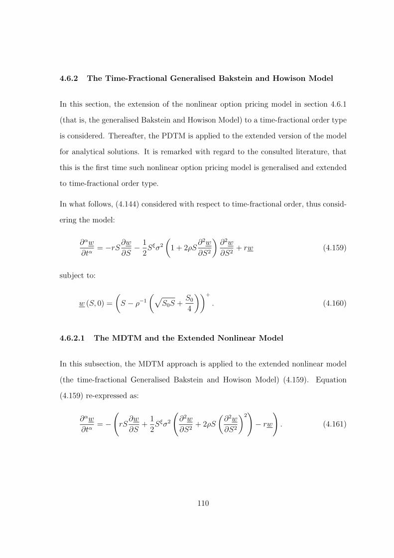
4.6.2 The Time-Fractional Generalised Bakstein and Howison Model

In this section, the extension of the nonlinear option pricing model in section 4.6.1

(that is, the generalised Bakstein and Howison Model) to a time-fractional order type

is considered. Thereafter, the PDTM is applied to the extended version of the model

for analytical solutions. It is remarked with regard to the consulted literature, that

this is the first time such nonlinear option pricing model is generalised and extended

to time-fractional order type.

In what follows, (4.144) considered with respect to time-fractional order, thus consid-

ering the model:

∂αw

∂tα= −rS ∂w

∂S− 1

2Sξσ2

(1 + 2ρS

∂2w

∂S2

)∂2w

∂S2+ rw (4.159)

subject to:

w (S, 0) =

(S − ρ−1

(√S0S +

S0

4

))+

. (4.160)

4.6.2.1 The MDTM and the Extended Nonlinear Model

In this subsection, the MDTM approach is applied to the extended nonlinear model

(the time-fractional Generalised Bakstein and Howison Model) (4.159). Equation

(4.159) re-expressed as:

∂αw

∂tα= −

(rS∂w

∂S+

1

2Sξσ2

(∂2w

∂S2+ 2ρS

(∂2w

∂S2

)2)− rw

). (4.161)

110

At projection, the transformation of (4.161) using PDTM yields the following:

PDT

[∂αw

∂t= −

(rS∂w

∂S+

1

2Sξσ2

(∂2w

∂S2+ 2ρS

(∂2w

∂S2

)2)− rw

)]. (4.162)

and

PDT

[w (S, 0) = max

(S − ρ−1

(√S0S +

S0

4

), 0

)]. (4.163)

Thus, the following is obtained:

Γ (1 + α (1 + k))

Γ (1 + αk)H (S, k + 1) = −

(rS∂H (S, k)

∂S− rH (S, k)

+1

2Sξσ2

(∂2H (S, k)

∂S2+ 2ρS

k∑n=0

∂2H (S, n)

∂S2

∂2H (S, k − n)

∂S2

)).

(4.164)

As such,

H (S, k + 1) =− Γ (1 + αk)

Γ (1 + α (1 + k))

(rS∂H (S, k)

∂S− rH (S, k)

+1

2S2σ2

(∂2H (S, k)

∂S2+ 2ρS

k∑n=0

∂2H (S, n)

∂S2

∂2H (S, k − n)

∂S2

) (4.165)

subject to:

H ((S, 0)) = max

(S − ρ−1

(√S0S +

S0

4

), 0

). (4.166)

For k = 0, we have:

H (S, 1) = − 1

Γ (1 + α)

(rS∂H (S, 0)

∂S− rH (S, 0)

+1

2Sξσ2

(∂2H (S, 0)

∂S2+ 2ρS

∂2H (S, 0)

∂S2

∂2H (S, 0)

∂S2

)).

(4.167)

111

For k = 1, the following is obtained:

H (S, 2) = − Γ (1 + α)

Γ (1 + 2α)

(rS∂H (S, 1)

∂S− rH (S, 1)

+1

2Sξσ2

(∂2H (S, 1)

∂S2+ 2ρS

1∑n=0

∂2H (S, n)

∂S2

∂2H (S, 1− n)

∂S2

))

= − Γ (1 + α)

Γ (1 + 2α)

(rS∂H (S, 1)

∂S− rH (S, 1)

+1

2Sξσ2

(∂2H (S, 1)

∂S2+ 4ρS

∂2H (S, 0)

∂S2

∂2H (S, 1)

∂S2

)).

(4.168)

For k = 2, the following is obtained:

H (S, 3) = −Γ (1 + 2α)

Γ (1 + 3α)

(rS∂H (S, 2)

∂S− rH (S, 2)

+1

2Sξσ2

(∂2H (S, 2)

∂S2+ 2ρS

2∑n=0

∂2H (S, n)

∂S2

∂2H (S, 2− n)

∂S2

))

= −Γ (1 + 2α)

Γ (1 + 3α)

rS∂H (S, 2)

∂S− rH (S, 2) +

1

2Sξσ2

(∂2H (S, 2)

∂S2

)+Sξ+1σ2ρ

(2∂2H (S, 0)

∂S2

∂2H (S, 2)

∂S2+∂2H (S, 1)

∂S2

∂2H (S, 1)

∂S2

).

(4.169)

For k = 3, the following is obtained:

H (S, 4) = −Γ (1 + 3α)

Γ (1 + 4α)

(rS∂H (S, 3)

∂S− rH (S, 3)

+1

2Sξσ2

(∂2H (S, 3)

∂S2+ 2ρS

3∑n=0

∂2H (S, n)

∂S2

∂2H (S, 3− n)

∂S2

))

= −Γ (1 + 3α)

Γ (1 + 4α)

(rS∂H (S, 3)

∂S− rH (S, 3) +

1

2Sξσ2∂

2H (S, 3)

∂S2

+1

2Sξσ2

(4ρS

(∂2H (S, 0)

∂S2

∂2H (S, 3)

∂S2+∂2H (S, 1)

∂S2

∂2H (S, 2)

∂S2

))).

(4.170)

112

For k = 4, the following is obtained:

H (S, 5) = −Γ (1 + 4α)

Γ (1 + 5α)

(rS∂H (S, 4)

∂S− rH (S, 4)

+1

2Sξσ2

(∂2H (S, 4)

∂S2+ 2ρS

4∑n=0

∂2H (S, n)

∂S2

∂2H (S, 4− n)

∂S2

))

= −Γ (1 + 4α)

Γ (1 + 5α)

(rS∂H (S, 4)

∂S− rH (S, 4) +

1

2Sξσ2

(∂2H (S, 4)

∂S2

+4ρS

(∂2H (S, 0)

∂S2

∂2H (S, 4)

∂S2+∂2H (S, 1)

∂S2

∂2H (S, 3)

∂S2+

1

2

(∂2H (S, 2)

∂S2

)2))

.

(4.171)

....

In general, for m ≥ 1, m ∈ N, the following is obtained:

H (S,m) = −Γ (1 + α (m− 1))

Γ (1 + αm)

(rS∂H (S,m− 1)

∂S− rH (S,m− 1)

+1

2S2σ2

(∂2H (S,m− 1)

∂S2+ 2ρS

m−1∑n=0

∂2H (S, n)

∂S2

∂2H (S,m− n− 1)

∂S2

).

(4.172)

4.6.2.2 Numerical Illustration and Applications

In this subsection, two cases are considered. Case 4.6.3.2.1 has two examples with

time-integer order while Case 4.6.3.2.2 has three examples with time-fractional order.

Equation (4.132) and (4.133) recalled as follows:

w (S, t) = w = S − ρ−1√S0

(√S exp

(r + σ2

4

2

)t+

√S0

4exp

(r +

σ2

4

)t

)

113

and

w (S, 0) = max

(S − ρ−1

(√S0S +

S0

4

), 0

)

respectively. For numerical illustration, some examples for different values of S, t,

and α over fixed values for the other parameters are considered. Hence, for r = 0.06,

|ρ| = 0.01, σ = 0.4, ξ = 2 and S0 = 4, the exact solution and initial condition are as

follows as:

w (S, t) = S + 200

(√S exp

(t

20

)+

1

2exp

(t

10

))(4.173)

and

w (S, 0) = S + 200√S + 100. (4.174)

Thus, by applying the MDTM with the above parameters, the following are obtained:

H (S, 0) = 100 + 200√S + S, (4.175)

H (S, 1) =1

2500Γ (1 + α)

(5000− 2500S1/2 − 75S + 600S2 + 1200S5/2 + 6S3

),

(4.176)

114

H (S, 2) =1

312500Γ (1 + 2α)

−125000 + 31250S1/2 + 5625S − 240000S3/2

−1080000S2 − 697200S5/2 − 5400S3

+3600S4 + 7200S9/2 + 36S5

,

(4.177)

....

Whence,

w (S, t) =∞∑h=0

H (S, h) thα

= H (S, 0) +H (S, 1) tα +H (S, 2) t2α +H (S, 3) t3α + · · ·

=(

100 + 200√S + S

)+

(1

2500Γ (1 + α)

(5000− 2500S1/2 − 75S + 600S2 + 1200S5/2 + 6S3

))tα

+

1

312500Γ (1 + 2α)

(−125000 + 31250S1/2 + 5625S − 240000S3/2

−1080000S2 − 697200S5/2 − 5400S3 + 3600S4 + 7200S9/2 + 36S5)t2α + · · · .

(4.178)

Based on (4.178), two Cases viz: Case 4.6.3.2.1 and Case 4.6.3.2.2 for integer and

time-fractional order are considered respectively. Tables 4.4-4.8 are for the compari-

son of solutions in line with their relative absolute errors (all for cases 4.6.3.2.1 and

4.6.3.2.2) as thus specified as follows: Table 4.4 and Table 4.5 are for Case 4.6.3.2.1

for an integer power of the time parameter. In a similar way, Tables 4.6-4.8 are

for Case 4.6.3.2.2 for fractional powers of the time parameter. Also, we present in

comparison, the exact and the approximate solutions for different values of t and α.

115

Table 4.4: The solutions of Case 4.6.3.2.1 at t = 0, and α = 1

S w (exact) w (approx) Rel. error0.5 241.92136 241.92136 0.0000000001.0 301.00000 301.00000 0.0000000001.5 346.44900 346.44898 5.77286E-082.0 384.84280 384.84272 2.07877E-072.5 418.72780 418.72777 7.16456E-083.0 449.41020 449.41017 6.67542E-083.5 477.66580 477.66574 1.25611E-074.0 504.00000 504.00000 0.0000000004.5 528.76410 528.76407 5.67361E-085.0 552.21360 552.21360 0.0000000005.5 574.54160 574.54158 3.48104E-086.0 595.89800 595.89795 8.3907E-086.5 616.40200 616.40196 6.48927E-087.0 636.15030 636.15027 4.71587E-087.5 655.22260 655.22256 6.1048E-08

116

Table 4.5: The solutions of Case 4.6.3.2.1 at t = 0.5, α = 1

S w (exact) w (approx) Rel. error0.5 250.62857 243.22119 0.0295552101.0 311.19020 301.95640 0.0296725281.5 357.77700 347.18204 0.0296133072.0 397.13010 385.49469 0.0292987362.5 431.86030 419.48813 0.0286485473.0 463.30670 450.53158 0.0275737863.5 492.26490 479.47976 0.0259720734.0 519.25320 506.93393 0.0237249774.5 544.63150 533.35939 0.0206967655.0 568.66200 559.14593 0.0167341415.5 591.54260 584.64223 0.0116650436.0 613.42690 610.17683 0.0052982196.5 634.43730 636.07195 0.0025765357.0 654.67290 662.65295 0.0121893707.5 674.21540 690.25510 0.023790172

117

Table 4.6: The solutions of Case 4.6.3.2.2 for t = 0.5 & α = 0.5

S w (exact) w (approx) Rel. error0.01 125.64342 123.22544 0.0192447800.02 134.14750 131.45494 0.0200716380.03 140.67510 137.77139 0.0206412510.04 146.17980 143.09741 0.0210862920.05 151.03060 147.79036 0.0214541950.06 155.41710 152.03352 0.0217709630.07 159.45170 155.93576 0.0220501880.08 163.20770 159.56801 0.0223009700.09 166.73610 162.97956 0.0225298540.10 170.07380 166.20626 0.0227403630.11 173.24890 169.27521 0.0229363070.12 176.28310 172.20744 0.0231199700.13 179.19370 175.01969 0.0232932850.14 181.99470 177.72552 0.0234577160.15 184.69770 180.33610 0.0236148040.16 187.31240 182.86079 0.0237656980.17 189.84680 185.30748 0.023910437

118

Table 4.7: The solutions of Case 4.6.3.2.2 for t = 0.5 & α = 1.5

S w (exact) w (approx) Rel. error0.01 125.64342 121.02823 0.0367324450.02 134.14750 129.30043 0.0361323920.03 140.67510 135.65022 0.0357197540.04 146.17980 141.00492 0.0354007870.05 151.03060 145.72370 0.0351379120.06 155.41710 149.99079 0.0349144980.07 159.45170 153.91560 0.0347196050.08 163.20770 157.56945 0.0345464710.09 166.73610 161.00186 0.0343911130.10 170.07380 164.24889 0.0342493080.11 173.24890 167.33777 0.0341192930.12 176.28310 170.28963 0.0339991180.13 179.19370 173.12131 0.0338872960.14 181.99470 175.84644 0.0337826320.15 184.69770 178.47625 0.0336845020.16 187.31240 181.02014 0.0335923300.17 189.84680 183.48606 0.033504594

119

Table 4.8: The solutions of Case 4.6.3.2.2 for t = 1 & α = 2.5

S w (exact) w (approx) Rel. error0.01 125.64342 120.21220 0.0432272540.02 134.14750 128.50205 0.0420839000.03 140.67510 134.86540 0.0412987090.04 146.17980 140.23152 0.0406915320.05 151.03060 144.96038 0.0401919880.06 155.41710 149.23655 0.0397675030.07 159.45170 153.16972 0.0393973850.08 163.20770 156.83132 0.0390691130.09 166.73610 160.27099 0.0387745070.10 170.07380 163.52487 0.0385064010.11 173.24890 166.62024 0.0382609070.12 176.28310 169.57828 0.0380343890.13 179.19370 172.41585 0.0378241530.14 181.99470 175.14662 0.0376279090.15 184.69770 177.78186 0.0374441050.16 187.31240 180.33096 0.0372716380.17 189.84680 182.80190 0.037108342

120

Table 4.4 shows the exact solution in column 2, the approximate solution in column

3, and the corresponding relative absolute errors in column 4 for t = 0, α = 1 and

S ∈ [0, 5]. Table 4.5 shows the exact solution in column 2, the approximate solution

in column 3, and the corresponding relative absolute errors in column 4 for t = 0.5,

α = 1 and S ∈ [0, 5]. Table 4.6 shows the exact solution in column 2, the approximate

solution in column 3, and the corresponding relative absolute errors in column 4 for

t = 0.5, α = 0.5 and S ∈ [0, 5]. Table 4.7 shows the exact solution in column 2, the

approximate solution in column 3, and the corresponding relative absolute errors in

column 4 for t = 0.5, α = 1.5 and S ∈ [0, 5]. Table 4.8 shows the exact solution

in column 2, the approximate solution in column 3, and the corresponding relative

absolute errors in column 4 for t = 1, α = 2.5 and S ∈ [0, 5].

Remark 4.6.2.3

In subsection 4.6.2, a time-fractional nonlinear transaction-cost model for stock op-

tion valuation in an illiquid market setting driven by a relaxed Black-Scholes model

assumption was considered. The considered case here is an extension of the nonlin-

ear model in subsection 4.6.1. The approximate-analytical solutions obtained via the

PDTM showed that the results in subsection 4.6.1 and those of Gonzalez-Gaxiola et

al. (2015) are special cases of this present extension.

4.7 Discussion and Summary of Results

Here, a concise discussion and summary of the research results in relation to the

associated objectives are presented. For more clarification and illustration, tables and

graphs are used at different stages.

121

4.7.1 The Transformed Black-Scholes Model

For the robustness of the proposed Transformed Black-Scholes Model (TBSM) in sec-

tion 4.2.1, three (3) sets of obtained solutions viz: the exact solution, the approximate

solution, and the proposed theoretical solution were compared. These solutions are

presented in Table 4.9, where MDTM

∗ (z) denotes approximate solution via DTM and

MP

∗ (z) denotes proposed theoretical solution. The absolute errors in both cases are

respectively defined as:

Abs Error : MDTM

∗ (z) =∣∣∣Exact Solution−MDTM

∗ (z)∣∣∣

and

Abs Error : MP

∗ (z) =∣∣∣Exact Solution−MP

∗ (z)∣∣∣

122

Table 4.9: The solutions of the TBSM and their absolute errors

zExactsolution

MDTM

∗ (z) MP

∗ (z)Abs Error :

MDTM

∗ (z)

Abs Error :

MP

∗ (z)1.0 1.166054 1.164705 1.166054 0.00134876 1.51796E-091.1 1.299419 1.297003 1.299419 0.00241637 1.54226E-091.2 1.434336 1.430218 1.434336 0.00411742 1.54817E-091.3 1.569919 1.563193 1.569919 0.00672601 1.53075E-091.4 1.705042 1.694444 1.705042 0.01059818 1.48408E-091.5 1.838290 1.822103 1.838290 0.01618656 1.40113E-091.6 1.967908 1.943852 1.967908 0.02405591 1.27359E-091.7 2.091749 2.056850 2.091749 0.03489897 1.09159E-091.8 2.207197 2.157645 2.207197 0.04955222 8.43522E-101.9 2.311097 2.242086 2.311097 0.06901105 5.15711E-102.0 2.399660 2.305216 2.399660 0.09444344 9.20788E-112.1 2.468361 2.341160 2.468361 0.12720134 4.46218E-102.2 2.511821 2.342993 2.511821 0.16882864 1.12124E-092.3 2.523668 2.302604 2.523668 0.22106420 1.9588E-092.4 2.496381 2.210543 2.496381 0.28583858 2.98902E-092.5 2.421110 2.055848 2.421110 0.36526218 4.247E-092.6 2.287467 1.825864 2.287467 0.46160279 5.77366E-092.7 2.083291 1.506041 2.083291 0.57724954 7.61657E-092.8 1.794375 1.079715 1.794375 0.71466030 9.83099E-09

123

Note: Table 5.9 shows the relationship between these solutions as presented in columns

2, 3, and 4, respectively. Similarly, in the last two columns, the absolute errors between

the solutions are displayed. It is obvious that the theoretical solution (in column 4)

converges faster to the exact solution (in column 2). It is noticed that our results agree

with those of Ugbebor et al. (2001) at φ1 = 12; hence, their model is a particular type

of this present model. Therefore, the proposed model is very robust and reliable.

4.7.2 The Generalised Black-Scholes Model

The generalised Black-Scholes Model via the CEV SDEs in section 4.3 for two cases

(with and without dividend yield parameters) is discussed here.

4.7.2.1 Comparison of the SDE Models (BSM and CEV-BSM)

This subsection discusses by comparing the fundamental features of the associated

models presented in section 4.3 as follows.

Let SN∗ and S∗ be the solutions of the SDEs in (4.39) and (2.2) , indicating no

dividend and dividend yields respectively. Suppose further that V BSM0 denotes the

volatility of the Black-Scholes model, V CEVM0 is the volatility of the CEV model

without dividend yield, V CEVM0∗ is the volatility of the CEV model with dividend

yield, V arBSM the variance of the Black-Scholes model, V ar

CEVM the variance of the CEV

model without dividend yield, V ar∗CEVM the variance of the CEV model with dividend

yield, mN∗CEVM the drift term of the CEV model without dividend yield, and m∗CEVM

the drift term of the CEV model with dividend yield. Then, the following are deduced

easily.

124

For volatilities:

V BSM0 = σ, V CEVM

0 = σSξ2−1, and V CEVM

0∗ = σ∗Sξ2−1∗ .

For the variances:

V arBSM = σ2, V ar

CEVM = σ2Sξ−2, and V ar∗CEVM = σ2

∗Sξ−2∗ .

For the mean parameters:

mN∗CEVM = µ, and m∗CEVM = µ− q.

Note: In both cases of the governing SDEs; with or without dividend parameter, it is

clear that the variances V arCEVM = g (σ, S∗) and V ar∗

CEVM = h (σ, SN∗) are functions of

the underlying asset prices SN∗ and S∗ respectively. This implies that the stock price

volatilities in both cases are variable functions. This result is of immense contribution

in the generalisation of the classical Black-Scholes pricing model as clearly depicted

in section 4.3.

4.7.3 Cases of the Generalised Bakstein and Howison Model - Section

4.6.1

The aspect of the result discussion here is on the solution of the generalised Bakstein

and Howison Model. To do this, reference is made to the numerical illustration

presented in Case 4.6.1.2.2 in subsection 4.6.1.1. Thus, the approximate and the

exact solutions are displayed in Figure 4.15 and Figure 4.16 respectively.

125

Figure 4.15: Exact solution for Case 4.6.1.2.2

126

Figure 4.16: Approximate solution for Case 4.6.1.2.2

127

The results are obtained with less computational time while still maintaining high

level of accuracy. In addition, these results conform to the associated exact solution

obtained by Esekon (2013) and the approximate solutions obtained by Gonzalez-

Gaxiola et al. (2015) using the Adomian decomposition method.

4.7.4 The Generalised Bakstein and Howison Model: Time-fractional

case - Section 4.6.2

This subsection discusses the solution of the time-fractional generalised Bakstein and

Howison Model. To do this, reference is made to the numerical illustration in sub-

section 4.6.2.1. Figure 4.17 and Figure 4.18 are for Case 4.6.3.2.1 for an integer

power of the time parameter. In a similar way, Figures 5.5-5.7 are for Case 4.6.3.2.2

for fractional powers of the time parameter. Also, in comparison, the exact and the

approximate solutions for different values of t and α are presented.

128

Figure 4.17: Solutions of Case 4.6.3.2.1 using Table 4.4

129

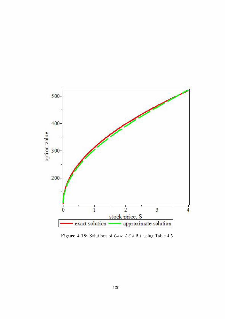
Figure 4.18: Solutions of Case 4.6.3.2.1 using Table 4.5

130

Figure 4.19: Solutions of Case 4.6.3.2.2 using Table 4.6

131

Figure 4.20: Solutions of Case 4.6.3.2.2 using Table 4.7

132

Figure 4.21: Solutions of Case 4.6.3.2.2 using Table 4.8

133

In Figure 4.17, the exact and the approximate solutions of the solved problem in Case

4.6.3.2.1 for t = 0 and α = 1 are presented. This is with respect to Table 4.4. In

Figure 4.18, the exact and the approximate solutions of the solved problem in Case

4.6.3.2.1 for t = 0.5 and α = 1 are presented. This is with respect to Table 4.5. In

Figure 4.19, the exact and the approximate solutions of the solved problem in Case

4.6.3.2.2 for t = 0.5 and α = 0.5 are presented. This is with respect to Table 4.6. In

Figure 4.20, the exact and the approximate solutions of the solved problem in Case

4.6.3.2.2 for t = 0.5 and α = 1.5 are presented. This is with respect to Table 4.7. In

Figure 4.21, the exact and the approximate solutions of the solved problem in Case

4.6.3.2.2 for t = 1 and α = 2.5 are presented. This is with respect to Table 4.5.

Remark 4.7.1

In section 4.7.4, the study considered a time-fractional nonlinear transaction-cost

model for stock option valuation in an illiquid market setting driven by a relaxed

Black-Scholes model assumption. The case considered in this subsection is an exten-

sion of the nonlinear model in subsection 4.5.1. The approximate-analytical solutions

obtained via the PDTM showed that the results in subsection 4.5.1 and those of

Gonzalez-Gaxiola et al. (2015) are particular cases of this present extension. It is

also note that the fractional time parameter α, serves as a control parameter since

the diffusion of the stock option price relies on the history of the price.

134

CHAPTER FIVE

CONCLUSION AND RECOMMENDATIONS

5.1 Introduction

In this chapter, the general summary and conclusion of the research work are pre-

sented. Recommendations and further areas of research are also made and suggested

respectively.

5.2 Conclusion

In this thesis, some established conditions for transforming the classical Black-Scholes

model for stock option valuation from its PDE form to an equivalent ODE form

have been considered. Consequently, a proposition regarding the theoretical value of

stock options was given, and a relatively new approximate-analytical technique was

proposed for the solution of the Transformed Black-Scholes Model (TBSM). Test cases

showed that obtained results agreed with the exact solution.

The study proposed CEV-Black-Scholes model for stock option valuation. The model

was derived in two forms as a generalisation of the classical Black-Scholes pricing

model using the CEV stochastic dynamics. In the first form, the concentration was on

the case without a dividend yield parameter; thereafter, the case with a dividend yield

parameter was incorporated. These models served as alternatives to the traditional

lognormal model for stock prices. In CEV model, the price variations of the underlying

asset are negatively correlated with variations in the level of volatility; this helps in

reducing the known volatility smile effects of the lognormal model. The key merit

of these models is that the stock price volatility is a function of the underlying asset

135

price but not a constant as assumed in the classical Black-Scholes pricing model.

In considering the European Option, the computational method: PDTM was suc-

cessfully applied to the Black-Scholes model for European Option Valuation (to the

best knowledge of the researcher, such application has not been considered in litera-

ture). The obtained solutions of the solved problems were expressed in simple forms

of convergent series as no linearization or perturbation is needed. These computed

results denote the analytical values of the associated European call options. The same

technique can be applied to European put options. In addition, the study provided

an accurate and exact solutions to the classical Black-Scholes model for stock option

valuation by the means of He’s polynomials. This technique gives the exact solution

of the solved problem in a very simple and quick manner even with less computational

work while still maintaining high level of accuracy.

With regard to the time-fractional Black-Scholes model for stock option valuation (an

extension of the classical Black-Scholes equations in time-fractional form), analyti-

cal solutions were obtained via the proposed relatively novel computational Method

(PDTM). The results obtained converged faster to their exact form of solutions (even

without giving up accuracy). It was remarked, to the best of the researcher’s knowl-

edge, that this proposed technique has not been reported in literature for solving

time-fractional Black-Scholes equations. This therefore, showed that the result in

subsection 4.4.1 is a special case of this present work for α = 1. Thus, the time-

fractional Black-Scholes equation for stock option valuation is a generalisation of the

classical Black-Scholes equations for European option valuation at order, α = 1.

In an extensive manner, the Bakstein and Howison model: a nonlinear transaction-

cost model for stock prices in an illiquid market, obtained when the constant volatil-

ity assumption of the classical linear Black-Scholes option pricing model was relaxed

136

through the inclusion of transaction cost was studied. Thereafter, the study gener-

alised and extended this nonlinear option pricing model to a time-fractional ordered

form, and obtained approximate-analytical solutions for both forms. Two cases with

five examples: case 1 with two examples for time-integer order, and case 2 with three

examples for time-fractional order were considered. The obtained results conformed

with the associated exact solutions obtained by Esekon (2013), and showed that the

work of Gonzalez-Gaxiola et al. (2015) using the Adomian decomposition method is

a particular case of this present work when α = 1.

5.3 Contributions to Knowledge

The following contributions are made to the body of knowledge:

(i) a stock option valuation model where the drift coefficient (rate of return) is a

non-fixed constant parameter has been derived, and a approximate-analytical

solution is provided;

(ii) the classical Black-Scholes option pricing model is generalised via a constant

elasticity of variance stochastic dynamics thereby addressing the assumption of

the constant volatility in the Black-Scholes Option Pricing Model;

(iii) analytical solutions of the Black–Scholes pricing model for European option

valuation are obtained via the proposed approximate-analytical methods;

(iv) the nonlinear transaction cost model of Bakstein and Howison (2003) for stocks

valuation is generalised, and analytical solution is provided via a proposed

approximate-analytical method;

(v) the generalised Bakstein and Howison model (2003) for stocks valuation has

been extended to a time-fractional order form; and

137

(vi) an analytical solution of the extended generalised model in (v) is obtained using

the MDTM.

5.4 Recommendations

‘Timeshare’ as a term in a business setting refers to an arrangement where joint

owners possess the right to a property on the ground of time-sharing agreement among

them. Meanwhile, in fractional ownership style of trade, business owners are entitled

to purchase a fixed time period share (mainly on monthly basis). It is therefore

recommended that:

(i) the time-fractional model be adopted in fractional ownership style of stock op-

tion valuation for effective and efficient time management;

(ii) the nonlinear model be adopted in an Employer-Employee stock option system

since dividend yield parameter is incorporated; and

(iii) the constant elasticity parameter in the nonlinear model enlarges the scope of

operation of the classical linear Black-Scholes model.

5.5 Open Problems

Basically, this study proposed stock option valuation model via the application of the

constant elasticity of variance dynamics with or without dividend yield. This model

(CEV-BSM) acts as a geralisation and extension of the classical Black-Scholes option

valuation model. Hence, for further research,

(a) the CEV-BSM could be extended to fractional order both in time and space

as a generalisation, and the approximate-analytical solutions of the resulting

138

PDEs for option valuation be obtained in a similar way using the proposed

approximate-analytical methods in this work.

(b) In addition, the generalised Bakstein and Howison nonlinear stock option model

was only with regard to time-fractional order; this could be considered with

respect to space-fractional order.

139

REFERENCES

Acharya, V. and Pedersen, L. H. (2005). Asset pricing with liquidity risk. Journal of

Financial Economics, 77 (2): 375-410.

Adebiyi, A. A., Adewumi, A. O. and Ayo, C. K. (2014). Comparison of ARIMA

and artificial neural network models for stock price prediction. Journal of Applied

Mathematics, 2014: 1-8. Article ID 614342.

Agliardi, R., Popivanov, P. and Slovova, A. (2013). On nonlinear Black-Scholes equa-

tions. Nonlinear Analysis and Differential Equations. 2013 (1): 75-81.

Ahmad, J., Shakeel, M., UI-Hassan, Q. M. and Mohyud-Din, S. T. (2013). Analyt-

ical solution of Black-Scholes model using fractional variational iteration method.

International Journal of Modern Mathematical Sciences, 5 (3): 133-142.

Ahmed, S. (2014). On the generalized fractional integrals of the generalized Mittag-

Leffler function. Springerplus, 3: 198-202. DOI:10.1186/2193-1801-3-198.

Akrami, M. H. and Erjaee, G. H. (2016). Numerical solutions for fractional Black-

Scholes option pricing equation, Global Analysis and Discrete Mathematics 1 (1):

9–14.

Akyildirim, E. and Soner, H. M. (2014). A brief history of mathematics in finance.

Borsa Istanbul Review 14 (1): 57–63.

Allahviranloo, T. and Behzadi, Sh. S. (2013). The use of iterative methods for solving

Black-Scholes equations. International Journal of Industrial Mathematics, 5 (1): 1-

11.

140

Amihud, Y. and Mendelson, H. (1986). Asset pricing and the bid-ask spread. Journal

of Financial Economics, 17: 223-249.

Arikoglu, A. and Ozkol, I. (2006). Solution of differential-difference equations by

using differential transform method. Applied Mathematical Computation, 181 (1):

153-162.

Arikoglu, A. and Ozkol, I. (2005). Solution of boundary value problems for integro-

differential equations by using differential transform method. Applied Mathematical

Computation, 168: 1145-1158.

Ayaz, F. (2003). On the two-dimensional differential transform method. Applied

Mathematical Computation, 143: 361-374.

Bachelier, L. (1900). Theorie de la speculation, Annales Scientifiques de L’Ecole Nor-

male Superieure, 17, 21-86. English translation by Boness A. J. (1964). In Cootner,

P. H. (ed.): The random character of stock market prices. Cambridge, MA: MIT

Press, 17-75.

Bakstein, D. and Howison, S. (2003). A non-arbitrage liquidity model with observable

parameters for derivatives. Mathematical Institute, Oxford University. Available at:

http://eprints.maths.ox.ac.uk/53/.

Beckners, S. (1980). The constant elasticity of variance model and its implications

for option pricing. The Journal of Finance, 35 (3): 661-673.

Black, F. and Scholes, M. (1973). The pricing of options and corporate liabilities.

Journal of Political Economy, 81 (3): 637-654.

Bohner, M., Sanchez, F. H. M. and Rodriguez, S. (2014). European call option

141

pricing using the Adomian decomposition method. Advances in Dynamical Systems

and Applications, 9 (1): 75-85.

Campbell, J. Y. and Shiller, R. J. (1988). Stock prices, earnings, and expected

dividends. Journal of Finance, 43: 661-676.

Carr, P., Geman, H., Madan, D.B. and Yor, M. (2002). The fine structure of asset

returns: an empirical investigation. The Journal of Business, 75 (2): 305-332.

Cen, Z. and Le, A. (2011). A robust and accurate finite difference method for a gener-

alized Black-Scholes equation. Journal of Computational and Applied Mathematics,

235 (13): 3728-3733.

Chen, C. K. and Ju, S. P. (2004). Application of differential transformation to tran-

sient advective-dispersive transport equation. Applied Mathematical Computation,

155 (1): 25-38.

Chen, W. and Wang, S. (2014). A penalty method for a fractional order parabolic

variational inequality governing American put option valuation. Computers and

Mathematics with Applications, 67 (1): 77–90.

Chernov, M., Gallant, A. R., Ghysels, E. and George Tauchen, G. (2003). Alternative

models for stock price dynamics. Journal of Econometrics, 116 (1-2): 225-257.

Cox, J. and Ross, S. (1976). The valuation of options for alternative stochastic

processes. Journal of Financial Economics, 3 (1-2): 145-166.

Delbaen, F. and Shirakawa, H. (2002). A note of option pricing for constant elasticity

of variance model. Asia-Pacific Financial Markets, 9 (2): 85-99.

142

Dura, D. and Mosneagu, A. M. (2010). Numerical approximation of Black-Scholes

equation. Analele Stiitifice Ale Universitatii “Al.i Cuza” Din Iasa (S.N.) Matematica,

Tomul 56: 39-64.

Duncan, T. E., Hu, Y. and Pasik-Duncan, B. (2000). Stochastic calculus for fractional

Brownian motion. SIAM Journal on Control and Optimization,38: 582-612.

Elbeleze, A. A., Kilicman, A. and Taib, B. M. (2013). Homotopy perturba-

tion method for fractional Black-Bcholes European option pricing equations using

Sumudu transform. Mathematical Problems in Engineering, (2013): 1-7.

Esekon, J. E. (2013). Analytic solution of a nonlinear Black-Scholes equation. Inter-

national Journal of Pure and Applied Mathematics, 82 (4): 547-555.

Fama, E. F. (1965). The behaviour of stock-market prices. Journal of Business, 38

(1): 34-105.

Fama, E. F. (1970). Efficient capital markets: A review of theory and empirical work.

Journal of Finance, 25 (2): 383–417.

Fornari, F. and Mele, A. (1997). Sign-and volatility-switching arch models: theory

and applications to international stock markets. Journal of Applied Econometrics,

12: 49-65.

Frey, R. and Patie, P. (2002). Risk management for derivatives in illiquid markets:

A simulation study. Advances in Finance and Stochastics, Springer, Berlin, 137-159.

ISBN 9783540434641.

Frey, R. and Stremme, A. (1997). Market volatility and feedback effects from dy-

namic hedging. Mathematical Finance, 4: 351-374.

143

Ghandehari, M. A. M. and Ranjbar, M. (2014). European option pricing of fractional

version of the Black-Scholes Model: Approach via expansion in series. International

Journal of Nonlinear Science, 17 (2): 105-110.

Ghorbani, A. (2009). Beyond Adomian’s polynomials: He polynomials. Chaos, Soli-

tons and Fractals, 39 (3): 1486–1492.

Ghorbani, A. and Nadjfi, J. S. (2007). He’s homotopy perturbation method for cal-

culating Adomian’s polynomials. International Journal of Nonlinear Sciences and

Numerical Simulation, 8 (2): 229-332.

Gonzalez-Gaxiola, O., Ruız de Chavez, J. and Santiago, J. A. (2015). A nonlinear

option pricing model through the Adomian decomposition method. International

Journal of Applied and Computational Mathematics, 1 (2): 1-15.

Habib, A. (2011). The calculus of finance. Universities Press (India) Private Ltd.

ISBN 8173717230.

Hanna, M. (1976). A stock predictive model based on changes in ratios of short

interest to trading volume. The Journal of Financial and Quantitative Analysis, 11

(5): 857-872.

Hariharan, G., Padma, S., and Pirabaharan, P. (2013). An efficient wavelet based ap-

proximation method to time fractional Black-Scholes European option pricing prob-

lem arising in financial market. Applied Mathematical Sciences, 7 (69): 3445-3456.

He, J. H. (2003). Homotopy perturbation method: A new nonlinear analytical tech-

nique. Applied Mathematics and Computation, 135 (1): 73-79.

Henderson, D. and Plaschko, P. (2006). Stochastic differential equations in science

144

and engineering. World Scientific Publishing Co. Pte. Ltd, London. ISBN: 978-981-

4480-53-6.

Hsu, Y. L. Lin, T. I. and Lee, C. F. (2008). Constant elasticity of variance (CEV) op-

tion pricing model: Integration and detailed derivation. Mathematics and Computers

in Simulation, 79 (1): 60–71.

Hull, J. and White, A. (1987). The pricing of options on assets with stochastic

volatility. The Journal of Finance, 42 (2): 271-301.

Ibrahim, R. W. and Jalab, H. A. (2015). Existence of Ulam stability for iterative

fractional differential equations based on fractional entropy. Entropy, 17: 3172-3181.

Ito, K. (1946). On a stochastic integral equation. Proceedings of the Japan Academy,

22: 32-35.

Ito, K. (1951). On stochastic differential equations. Memoirs American Mathematical

Society, 4: 1-51. Doi.org/10.1090/memo/0004.

Jang, B. (2010). Solving linear and nonlinear initial value problems by the projected

differential transform method. Computer Physics Communications, 181 (5): 848-

854.

Jumarie, G. (2008). Stock exchange fractional dynamics defined as fractional ex-

ponential growth driven by (usual) Gaussian white noise: Application to fractional

Black-Scholes equations, Insurance: Mathematics and Economics, 42 (1): 271–287.

Keynes, J. M. (1971). A treatise on money: The pure theory of money. Johnson, E.

and Moggridge, D. (eds.) Macmillan, London, ISBN: 978-0-404-15000-6.

145

Kilbas, A. A., Srivastava, H. M. and Trujilo, J. J. (2006). Theory and applications

of fractional differential equations. 1st Edn. North-Holland Mathematical Studies,

Elsevier, Amsterdam. ISBN: 9780080462073.

Kobila, T. O. (1993). A class of solvable stochastic investment problems involving

singular controls. Stochastics and Stochastics Reports, 43: 29-63.

Kumar, S., Yildirin, A., Khan, Y., Jafari, H., Sayevand, K. and Wei, L. (2012).

Analytical solution of fractional Black-Scholes European option pricing equations

using Laplace transform. Journal of Fractional Calculus and Applications, 2 (8):

1-9.

Kumar, S., Kumar, D. and Singh, J. (2014). Numerical computation of fractional

Black-Scholes equation arising in financial market. Egyptian Journal of Basic and

Applied Sciences, 1: 177-183.

Lin, X., Yang, Z. and Song, Y. (2009). Short-term stock price prediction based on

echo state networks. Expert Systems with Applications, 36, 7313–7317.

Merdan, M. (2013). Numerical solution of the fractional-order Vallis systems using

multi-step differential transformation method. Applied Mathematical Modelling, 37

(8): 6025-6036.

Merton, R. (1973). Theory of rational option pricing. Bell Journal of Economics and

Management Science, 4: 141–183.

Merton, R. C., Brennan, M. J. and Schwartz, E. S. (1977). The valuation of American

put options. Journal of Finances, 32 (2): 449-462.

Mohyud-Din, S. T. (2011). Solution of troesch’s problem using He’s polynomials.

146

Revista de la Union Matematica Argentina, 52 (1): 143-148.

Momani, S., Odibat, Z., and Eturk, V. S. (2007). Generalized differential transform

method for solving a space- and time-fractional diffusion-wave equation. Physics

Letter A., 370 (5-6): 379-387.

Nazari, D. and S. Shahmorad (2010). Application of the fractional differential trans-

form method to fractional-order integro-differential equations with nonlocal bound-

ary conditions. Journal of Computational and Applied Mathematics, 234 (3): 883-

891.

Necula, C. (2008). Option pricing in a fractional Brownian motion environment.

Finance and Banking, Bucharest University of Economics, 94: 109-126.

Nelson, S. A. (1904). The A B C of options and arbitrage. The Wall Street Library,

VI, New York, 96p.

NGSE-Nigerian Stock Exchange, (2016). https://www.african-

markets.com/en/stock-markets/ngse/listed-companies. Retrived: May 31, 2016.

NGSEINDX:IND-Nigerian Stock Exchange All Share Index, (2016)

www.nse.com.ng/products/indices. Retrived: May 31, 2016.

Nkeki, C. I. (2011). On optimal portfolio management of the accumulated phase of

a defined contributory pension scheme. Unpublished Ph.D Thesis, Department of

Mathematics, University of Ibadan, Nigeria.

Onah, S. E. and Ugbebor, O. O. (1999). Solution of a two-dimensional stochastic

investment problem. Applied Mathematics and Computation, 98: 75-82.

147

Osborne, M. F. M. (1964). Brownian motion in the stock market. In: The random

character of stock market prices, P. H. Cootner (Editor). Cambridge, MA: MIT

Press, 100-128.

Owoloko, E. A. (2014). On the valuation of banks as growth enterprises. Unpublished

Ph.D Thesis, Department of Mathematics, Covenant University, Ota, Nigeria.

Owoloko, E. A. and Okeke, M. C. (2014). Investigating the imperfection of the B-S

Model: A case study of an emerging stock market. British Journal of Applied Science

and Technology, 4 (29): 4191-4200.

Peters, E. E. (1989). Fractal structure in the capital markets. Financial Analysts

Journal, 45 (4): 32-37.

Phaochoo, P., Luadsong, A. and Aschariyaphotha, N. (2016). A numerical study

of the European option by the MLPG method with moving kriging interpolation.

SpringerPlus, 5 : 305-318.

Podlubny, I. (1999). Fractional differential equations. Mathematics in Science and

Engineering, 198, 1st Edn. ISBN: 9780080531984.

Qiu, Y. and Lorenz, J. (2009). A nonlinear Black-Scholes equation. International

Journal of Business Performance and Supply Chain Modelling, 1 (1): 33-40.

Rapach, D. E. and Wohar, M. E. (2005). Valuation ratios and long-horizon stock

price predictability. Journal of Applied Economics, 20: 327-344.

Rashidi, M. M. (2009). The modified differential transform method for solving MHD

boundary-layer equations. Computer Physics Communications, 180 (11): 2210-

2217.

148

Ravi, K. A. S. V. and Aruna, K. (2008). Solution of singular two-point boundary

value problems using differential transform method. Physics Letter A, 372 (26):

4671-4673.

Ravi, K. A. S. V. and Aruna, K. (2012). Comparison of two dimensional DTM and

PDTM for solving Time- Dependent Emden-Fowler Type Equations. International

Journal of Nonlinear Science, 13 (2): 228-239.

Reiss, W. (1975). A note on stock market prices in Germany and the random walk

hypothesis. Kyklos, 28 (4): 878-883.

Samuelson, P. A. (1969). Lifetime portfolio selection by dynamic stochastic program-

ming. The Review of Economics and Statistics, 51 (3): 239-246.

Schoneburg, E. (1990). Stock price prediction using neural networks: A project

report. Neurocomputing, 2: 17-27.

Sen, A. K. (1988). An application of the Adomian decomposition method to the

transcient behaviour of a model of biochemical reaction. Journal of Mathematical

Analysis and Applications, 131: 232-245.

Shane, P. B. and Stock, T. (2006). Security analyst and stock market efficiency in

anticipating tax-motivated income shifting. The Accounting Review, 81 (1): 227-

250.

Shepp, L. (2002). A model for stock price fluctuations based on information. IEEE

Transactions on Information Theory, 48 (6): 1372-1378.

Song, J. Yin, F., Cao. X. and Lu, F. (2013). Fractional variational iteration method

versus Adomian’s decomposition method in some fractional partial differential equa-

149

tions. Journal of Applied Mathematics, (2013): 10 pages . Article ID: 392567.

Sprenkle, C. (1964). Warrant prices as indicators of expectations and preferences in

the random character of stock market prices, Cootner, P. (ed.) MIT Press, Cambridge

MA, 412-474.

Tari, A. and Shahmorad, S. (2011). Differential transform method for the system

of two-dimensional nonlinear Volterra integro-differential equations. Computers and

Mathematics with Applications, 61 (9): 2621-2629.

Uddin, M. K. S., Ahmed, M. and Bhowmik, S.K. (2013). A note on numerical solution

of linear Black-Scholes model. GANIT: Journal of Bangladesh Mathematical Society,

33: 103-115.

Ugbebor, O. O., Onah, E. S. and Ojowu, O. (2001). An empirical stochastic model

of stock price changes. Journal of the Nigeria Mathematical Society, 20: 95-101.

Wang, X.-T. (2010). Scaling and long-range dependence in option pricing I: Pricing

European option with transaction costs under the fractional Black-Scholes model.

Physica A, 389: 438-444.

Wu, J-L. and Hu, Y-H, (2011). Price–dividend ratios and stock price predictability.

Journal of forecasting, (wileyonlinelibrary.com).

Zhou, J. K. (1986). Differential transformation and its application for electrical cir-

cuits, Huazhong University Press, Wuhan, China.

150

APPENDIX A: MAPLE CODE FOR FIGURES (A1-A5)

A1: MAPLE CODE FOR FIGURES 4.1 and 4.2

FIGURE 4.1

Psoln=z+(3/20)*z∧2+(19/600)*z∧3-(71/8000)*z∧4-(5849/1200000)*z∧5-

(32107/12000000)*z∧6, z = 1 .. 2.5

dtm := z+(3/20)*z∧2+(19/600)*z∧3-(71/8000)*z∧4-(5849/1200000)*z∧5-

(32107/12000000)*z∧6

exact := exp((1/10*(4+sqrt(61)))*z)*(-(1/61)*sqrt(61)-1)+exp(-(1/10*(-

4+sqrt(61)))*z)*(-1+(1/61)*sqrt(61))+2*exp(z)

plot([-1.128036879*exp(1.181024968*z)-.8719631201*exp(-.3810249676*z)+2*exp(z),

z+(3/20)*z∧2+(19/600)*z∧3-(71/8000)*z∧4-(5849/1200000)*z∧5-(32107/12000000)*z∧6,

exp((1/10*(4+sqrt(61)))*z)*(-(1/61)*sqrt(61)-1)+exp(-(1/10*(-4+sqrt(61)))*z)*(-

1+(1/61)*sqrt(61))+2*exp(z)], z = 1 .. 2.4, labels = [”independent pa-

rameter: z”, ”solution: M(z)”], labeldirections = [”horizontal”, ”verti-

cal”], labelfont = [”ROMAN”, 12], linestyle = [solid, longdash, dashdot],

titlefont = [”ROMAN”, 12], thickness = 3, legend = [”proposed solution”,

”DTM solution”, ”exact solution”])

FIGURE 4.2

S := CEVProcess(s0, mu, sigma, xi);

Diffusion(S(t));

simplify(Drift(S(t)∧(2-xi)));

151

simplify(Diffusion(S(t)∧(2-xi)));

S := SamplePath(S(t), t = 0 .. T, timesteps = 100, replications = 10∧4);

The following set of examples estimates the distribution of

max(0, S(2)-1);

for different values of the elasticity parameter ExpectedValue(max(S(T)-1, 0), timesteps

= 100, replications = 10∧4);

xi := 2.0;

S1 := SampleValues(S(T), timesteps = 100, replications = 10∧4);

xi := 2.5;

S2 := SampleValues(S(T), timesteps = 100, replications = 10∧4);

xi := .1;

S3 := SampleValues(S(T), timesteps = 100, replications = 10∧4);

P1 := Statistics[FrequencyPlot](S1, range = 0 .. 3, bincount = 10, averageshifted =

5,

thickness = 3, color = red);

P2 := Statistics[FrequencyPlot](S2, range = 0 .. 3, bincount = 10, averageshifted =

5,

thickness = 3, color = black);

P3 := Statistics[FrequencyPlot](S3, range = 0 .. 3, bincount = 10, averageshifted =

5,

thickness = 3, color = green);

152

plots[display](P1,P2,P3,gridlines=true,tickmarks=[,5]);

A2: MAPLE CODE FOR FIGURES 4.3 & 4.4

FIGURE 4.3

V(x,t)=

-1.412646800*t+x-4.742163550*10∧(-63)*t∧28-2.213009657*10∧(-60)*t∧27-

9.958543459*10∧(-58)*t∧26-8.064113665*10∧(-102)*t∧42-5.644879565*10∧(-

99)*t∧41-3.857334369*10∧(-96)*t∧40-2.571556247*10∧(-93)*t∧39-1.671511560*10∧(-

90)*t∧38-1.058623988*10∧(-87)*t∧37-6.528181261*10∧(-85)*t∧36-3.916908757*10∧(-

82)*t∧35-2.284863441*10∧(-79)*t∧34-1.294755950*10∧(-76)*t∧33-7.121157724*10∧(-

74)*t∧32-3.797950787*10∧(-71)*t∧31-9.811372865*10∧(-66)*t∧29-1.962274573*10∧(-

68)*t∧30-2.045863932*10∧(-110)*t∧45-1.534397949*10∧(-107)*t∧44+

-1.125225163*10∧(-104)*t∧43-1.798070347*10∧(-52)*t∧24-4.315368832*10∧(-

55)*t∧25-7.192281387*10∧(-50)*t∧23-1.010915106*10∧(-44)*t∧21-2.757041199*10∧(-

47)*t∧22-1.179400957*10∧(-39)*t∧19-3.538202871*10∧(-42)*t∧20-1.120430909*10∧(-

34)*t∧17-3.734769697*10∧(-37)*t∧18-8.465477980*10∧(-30)*t∧15-3.174554241*10∧(-

32)*t∧16-4.938195487*10∧(-25)*t∧13-2.116369495*10∧(-27)*t∧14-6.538536619*10∧(-

16)*t∧9-3.923121971*10∧(-18)*t∧10-2.139884712*10∧(-20)*t∧11-1.069942356*10∧(-

22)*t∧12-1.525658544*10∧(-7)*t∧5-1.525658544*10∧(-9)*t∧6-1.307707324*10∧(-

11)*t∧7-9.807804929*10∧(-14)*t∧8-47.08822668-0.8475880802e-3*t∧3-0.1271382120e-

4*t∧4-0.4237940401e-1*t∧2 plot3d(x-25*exp(-0.6e-1)-(x-x+25*exp(-0.6e-

1))*(sum((0.6e-1*t)∧i/factorial(i), i = 1..10)), t = 0 .. 10, x = 0 .. 1000,

axes = boxed)

FIGURE 4.4 *vexact = x*(1-exp(0.6e-1*t))+(x-exp(-0.6e-1))*exp(0.6e-1*t); plot3d(x*(1-

153

exp(0.6e-1*t))+(x-exp(-0.6e-1))*exp(0.6e-1*t), t = 0 .. 10, x = 0 .. 1000, axes =

boxed);

A3: MAPLE CODE FOR FIGURES 4.7-4.12

FIGURE 4.7

w(x,t) = x∧3*exp(-6.5*t) plot3d(x∧3*exp(-6.5*t), t = 0 .. 9, x = 0 .. 2, axes =

boxed)

FIGURE 4.8 plot3d(x∧3*exp(-6.5*t), t = 0 .. 18, x = 0 .. 2, axes = boxed)

FIGURE 4.9

w(x,t exact) = (-1+exp(x))*exp(-2*t)+(1-exp(-2*x))*exp(x)

plot3d((-1+exp(x))*exp(-2*t)+(1-exp(-2*x))*exp(x), t = 0 .. 45, x = 0 .. 45, axes =

boxed)

FIGURE 4.10

plot3d((-1+exp(x))*exp(-2*t)+(1-exp(-2*x))*exp(x), t = 0 .. 80, x = 0 .. 45, axes =

boxed)

FIGURE 4.11

w(x,t) = x-25*exp(-0.6e-1)+(1-exp(0.6e-1*t))*(x-x+25*exp(-0.6e-1))

plot3d(x-25*exp(-0.6e-1)+(1-exp(0.6e-1*t))*(x-x+25*exp(-0.6e-1)), t = 0 .. 10, x =

0 .. 200,

154

axes = boxed)

FIGURE 4.12

plot3d(x*(1-exp(0.6e-1*t))+(x-25*exp(-0.6e-1))*exp(0.6e-1*t), t = 0 .. 10, x = 0 ..

400,

axes = boxed)

A4: MAPLE CODE FOR FIGURES 4.13-4.16

FIGURE 4.13

w(s,t) =-(1/25)*(2*s(-(50*(s+sqrt(s)))/s∧(5/2))∧2*s∧(9/2)*t-25*s∧(11/2)-

5000*s∧5-2500*s∧(9/2)-1200*s∧(5/2)*t∧2-4700*s∧2*t∧2-5900*s∧(3/2)*t∧2-

4800*s*t∧2-6300*t∧2*sqrt(s)-4000*t∧2)/s∧(9/2)

plot3d(((1/25)*(2*s(-(50*(s+sqrt(s)))/s∧(5/2))∧2*s∧(9/2)*t-25*s∧(11/2)-

5000*s∧5-2500*s∧(9/2)-1200*s∧(5/2)*t∧2-4700*s∧2*t∧2-5900*s∧(3/2)*t∧2-

4800*s*t∧2-6300*t∧2*sqrt(s)-4000*t∧2)/s∧(9/2)

), S = 0.1 .. 10, t = 0 .. 1, axes = boxed);

FIGURE 4.14

w(exact) = s+200*(sqrt(s)*exp((1/50)*t)+(1/2)*exp((1/100)*t))

plot3d(s+200*(sqrt(s)*exp((1/50)*t)+(1/2)*exp((1/100)*t)), S = .1 .. 10,

t = 0 .. 1, axes = boxed)

Figure 4.15

155

w(s,t exact) = s+200*(sqrt(s)*exp((1/20)*t)+(1/2)*exp((1/10)*t))

# 3D Plot s+200*s∧(1/2)*exp(1/20*t)+100*exp(1/10*t)

plot3d(s+200*s∧(1/2)*exp(1/20*t)+100*exp(1/10*t), t = 1 .. 2, s = 0.1

.. 5, axes = boxed);

Figure 4.16

w(s,t) =s+200*sqrt(s)+100+(-(3/50)*s*(1+100/sqrt(s))-(2/25)*s∧2*(-50/s∧(3/2)-

50/s∧2-(3/50)*s-12*sqrt(s)-6))*t+(-(3/100)*s*(-3/50-3/sqrt(s)-(4/25)*s*(-

50/s∧(3/2)-50/s∧2-(3/50)*s-12*sqrt(s)-6)-(2/25)*s∧2*(75/s∧(5/2)+100/s∧3-

3/50-6/sqrt(s)))-(1/25)*s∧2*(19/(2*s∧(3/2))+8/s∧2+(6/625)*s+(48/25)*sqrt(s)+24/25-

(8/25)*s*(75/s∧(5/2)+100/s∧3-3/50-6/sqrt(s))-(2/25)*s∧2*(-375/(2*s∧(7/2))-

300/s∧4+3/s∧(3/2))+(2*(19/(2*s∧(3/2))+8/s∧2+(6/625)*s+(48/25)*sqrt(s)+24/25-

(8/25)*s*(75/s∧(5/2)+100/s∧3-3/50-6/sqrt(s))-(2/25)*s∧2*(-375/(2*s∧(7/2))-

300/s∧4+3/s∧(3/2))))/sqrt(s)-(3/50)*s*(-(3/50)*s*(1+100/sqrt(s))-(2/25)*s∧2*(-

50/s∧(3/2)-50/s∧2-(3/50)*s-12*sqrt(s)-6))))*t∧2

plot3d(s+200*sqrt(s)+100+(-(3/50)*s*(1+100/sqrt(s))-(2/25)*s∧2*(-50/s∧(3/2)-

50/s∧2-(3/50)*s-12*sqrt(s)-6))*t+(-(3/100)*s*(-3/50-3/sqrt(s)-(4/25)*s*(-

50/s∧(3/2)-50/s∧2-(3/50)*s-12*sqrt(s)-6)-(2/25)*s∧2*(75/s∧(5/2)+100/s∧3-

3/50-6/sqrt(s)))-(1/25)*s∧2*(19/(2*s∧(3/2))+8/s∧2+(6/625)*s+(48/25)*sqrt(s)+24/25-

(8/25)*s*(75/s∧(5/2)+100/s∧3-3/50-6/sqrt(s))-(2/25)*s∧2*(-375/(2*s∧(7/2))-

300/s∧4+3/s∧(3/2))+(2*(19/(2*s∧(3/2))+8/s∧2+(6/625)*s+(48/25)*sqrt(s)+24/25-

(8/25)*s*(75/s∧(5/2)+100/s∧3-3/50-6/sqrt(s))-(2/25)*s∧2*(-375/(2*s∧(7/2))-

300/s∧4+3/s∧(3/2))))/sqrt(s)-(3/50)*s*(-(3/50)*s*(1+100/sqrt(s))-(2/25)*s∧2*(-

50/s∧(3/2)-50/s∧2-(3/50)*s-12*sqrt(s)-6))))*t∧2, t = 1 .. 2, s = .1 .. 5,

axes = boxed)

156

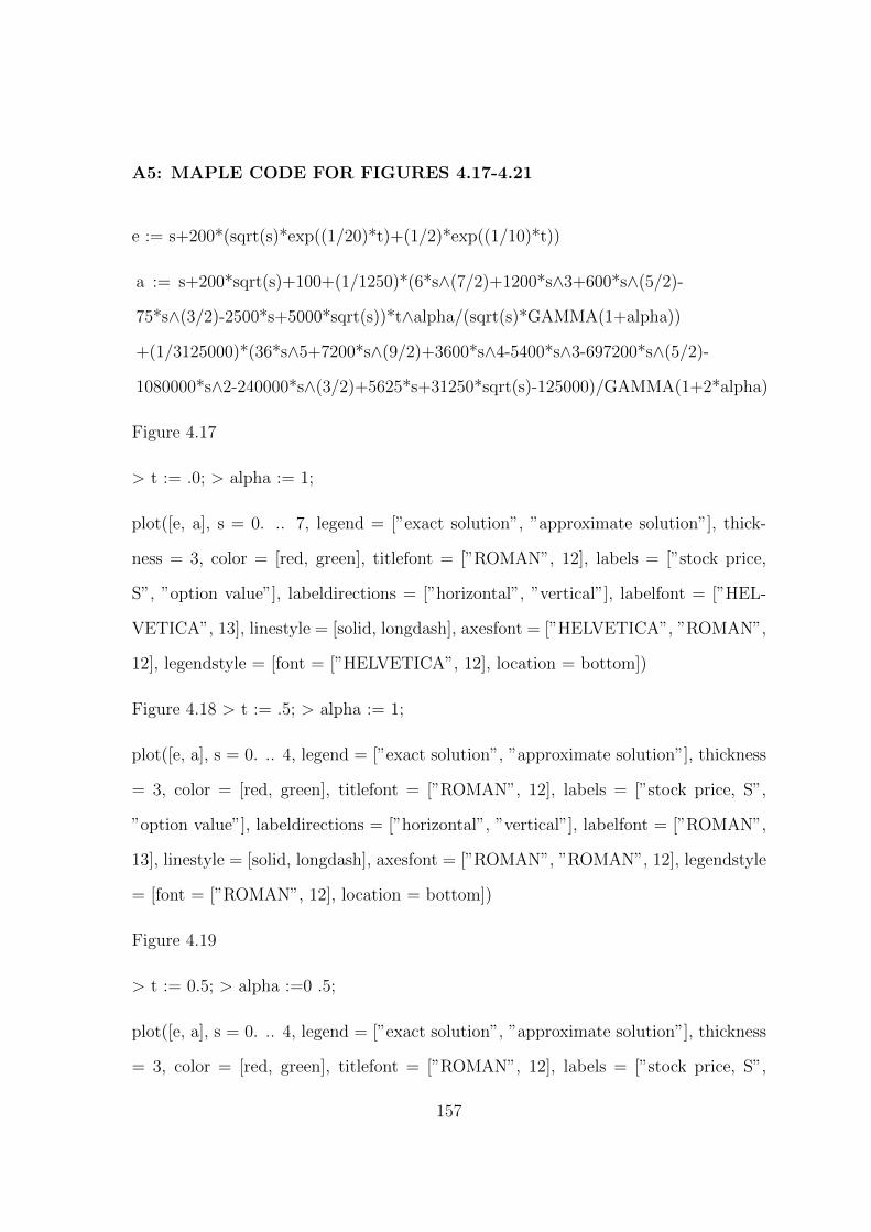
A5: MAPLE CODE FOR FIGURES 4.17-4.21

e := s+200*(sqrt(s)*exp((1/20)*t)+(1/2)*exp((1/10)*t))

a := s+200*sqrt(s)+100+(1/1250)*(6*s∧(7/2)+1200*s∧3+600*s∧(5/2)-

75*s∧(3/2)-2500*s+5000*sqrt(s))*t∧alpha/(sqrt(s)*GAMMA(1+alpha))

+(1/3125000)*(36*s∧5+7200*s∧(9/2)+3600*s∧4-5400*s∧3-697200*s∧(5/2)-

1080000*s∧2-240000*s∧(3/2)+5625*s+31250*sqrt(s)-125000)/GAMMA(1+2*alpha)

Figure 4.17

> t := .0; > alpha := 1;

plot([e, a], s = 0. .. 7, legend = [”exact solution”, ”approximate solution”], thick-

ness = 3, color = [red, green], titlefont = [”ROMAN”, 12], labels = [”stock price,

S”, ”option value”], labeldirections = [”horizontal”, ”vertical”], labelfont = [”HEL-

VETICA”, 13], linestyle = [solid, longdash], axesfont = [”HELVETICA”, ”ROMAN”,

12], legendstyle = [font = [”HELVETICA”, 12], location = bottom])

Figure 4.18 > t := .5; > alpha := 1;

plot([e, a], s = 0. .. 4, legend = [”exact solution”, ”approximate solution”], thickness

= 3, color = [red, green], titlefont = [”ROMAN”, 12], labels = [”stock price, S”,

”option value”], labeldirections = [”horizontal”, ”vertical”], labelfont = [”ROMAN”,

13], linestyle = [solid, longdash], axesfont = [”ROMAN”, ”ROMAN”, 12], legendstyle

= [font = [”ROMAN”, 12], location = bottom])

Figure 4.19

> t := 0.5; > alpha :=0 .5;

plot([e, a], s = 0. .. 4, legend = [”exact solution”, ”approximate solution”], thickness

= 3, color = [red, green], titlefont = [”ROMAN”, 12], labels = [”stock price, S”,

157

”option value”], labeldirections = [”horizontal”, ”vertical”], labelfont = [”ROMAN”,

13], linestyle = [solid, longdash], axesfont = [”ROMAN”, ”ROMAN”, 12], legendstyle

= [font = [”ROMAN”, 12], location = bottom])

Figure 4.20

> t := 0.5; > alpha := 1.5;

plot([e, a], s = 0. .. 4, legend = [”exact solution”, ”approximate solution”], thickness

= 3, color = [red, green], titlefont = [”ROMAN”, 12], labels = [”stock price, S”,

”option value”], labeldirections = [”horizontal”, ”vertical”], labelfont = [”ROMAN”,

13], linestyle = [solid, longdash], axesfont = [”ROMAN”, ”ROMAN”, 12], legendstyle

= [font = [”ROMAN”, 12], location = bottom])

Figure 4.21

> t := 1; > alpha := 2.5;

plot([e, a], s = 0. .. 7, legend = [”exact solution”, ”approximate solution”], thickness

= 3, color = [red, green], titlefont = [”ROMAN”, 12], labels = [”stock price, S”,

”option value”], labeldirections = [”horizontal”, ”vertical”], labelfont = [”ROMAN”,

13], linestyle = [solid, longdash], axesfont = [”ROMAN”, ”ROMAN”, 12], legendstyle

= [font = [”ROMAN”, 12], location = bottom])

158

APPENDIX BNGSEINDX Simulated Data (2000 - 2016): Figure 3.1

159

APPENDIX B Cont’d:

160

APPENDIX B Cont’d:

161

APPENDIX B Cont’d:

162

APPENDIX B Cont’d:

163