BBREAKREAK VVENEN AANALYSNALYSIISS

EE

AA PPRESENTATRESENTATIIONON BBYY,

RAVINDRA RAVINDRA BABUBABU

PGDM – 1PGDM – 1STST SEMSEM

INTRODUCTION.. Break-even analysis is a useful tool to study the relationship

between fixed costs, variable costs and returns.

Break even analysis gives the analysis of the Sales Volume where the Variable Costs and Fixed Costs of the Products are recovered.

You can use break-even analysis to determine how much product or service you need to sell at a specific price to meet all costs.

INTRODUCTION.

Break-even analysis is a mathematical formula that discloses how much output must be sold for the business to break even.

Break-even is reached when the money coming in equals the money going out.

BREAK EVEN POINT It may be defined as the level of sales at which

the total revenue is equal to total costs and the net income is zero.

It is the point of activity where total revenue and total expenses are equal.

This is also known as “No Profit and No Loss” zone.

Breakeven Point = Fixed Costs/(Selling Price per unit - Variable Cost per unit)

FIXED COSTCost that do not change when production or sales levels do change, such as rent, property tax, insurance, or interest expense. The fixed costs are summarized for a specific time period (generally one month).

VARIABLE COST

Variable costs are costs directly related to production units. Typical variable costs include direct labor and direct materials. The variable cost times the number of units sold will equal the Total Variable Cost. Total Variable costs plus Fixed costs make up the total cost of production.

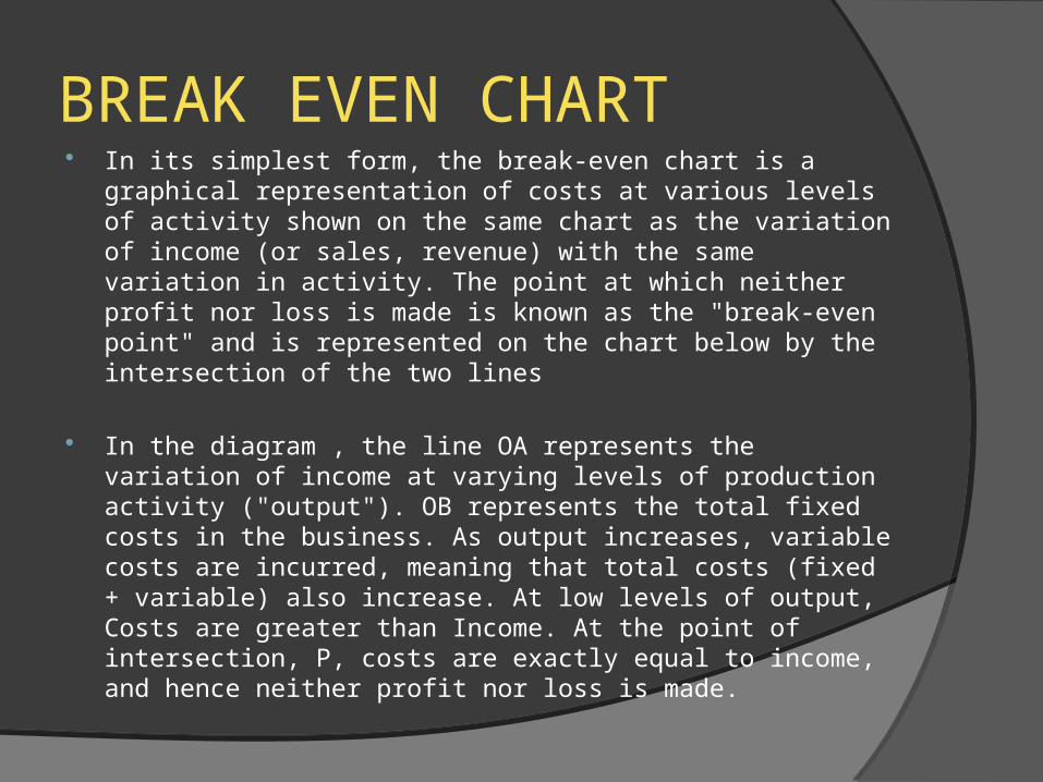
BREAK EVEN CHART In its simplest form, the break-even chart is a graphical

representation of costs at various levels of activity shown on the same chart as the variation of income (or sales, revenue) with the same variation in activity. The point at which neither profit nor loss is made is known as the "break-even point" and is represented on the chart below by the intersection of the two lines

In the diagram , the line OA represents the variation of income at varying levels of production activity ("output"). OB represents the total fixed costs in the business. As output increases, variable costs are incurred, meaning that total costs (fixed + variable) also increase. At low levels of output, Costs are greater than Income. At the point of intersection, P, costs are exactly equal to income, and hence neither profit nor loss is made.

BREAK EVEN CHART

COMPUTATION OF BREAK EVEN ANALYSIS

In the linear Cost-Volume-Profit Analysis model , the break-even point (in terms of Unit Sales (X)) can be directly computed in terms of Total Revenue (TR) and Total Costs (TC) as:

where:

TFC is Total Fixed Costs,

P is Unit Sale Price, and

V is Unit Variable Cost

LINEAR BREAK-EVEN ANALYSIS

• Over small enough range of output levels, TR and TC may be linear, assuming :– Constant selling price (MR)– Constant marginal cost (MC)– Firm produces only one product– No time lags between investment and resulting

revenue stream

LINEAR BEA EQUATION

ASSUME : TR=15Q, TFC=100, TVC=10Q.

THAT IS, IN TERMS OF TR AND TC FUNCTIONS,TR = TCHENCE,TC=TFC+TVC15Q = 100 + 10Q5Q = 100Q = 20

THUS, 20 IS THE BREAK-EVEN OUTPUT. GIVEN TR & TC FUNCTIONS, PRODUCTION BEYOND 20 UNITS WILL YIELD INCREASING PROFITS, (AT LEAST IN THE SHORT RUN).

TR 700

OP. PROFIT

TC 600

500 TVC

400 B

C& R

300

200 OP. LOSS

100 TFC

50

Q

10 20 30 40

output

LINEAR GRAPHLINEAR GRAPH

• The line TFC shows the total fixed cost and the line TVC shows the variable cost.• The line TC can be obtained also by a vertical summation of TFC and TVC at various levels of o/p. • The line TR shows the total revenue (TR) obtained with Q o/p.• The line TR intersects the line TC at point b. the point b shows that at Q, the firm’s total cost equals its total revenue. that is, at Q , TC breaks even with tr. point b is, therefore, the break even point and Q is the break-even level of o/p. • Below Q level of o/p, TC >TR. the vertical difference between TC and TR, (i.e., TC-TR) is known as operating loss. • Beyond Q, TR>TC, and TR- TC is known as operating profit. • It may thus be inferred that a firm producing a commodity under cost and revenue conditions mentioned above must produce atleast Q units to make its total cost and total revenue break even.

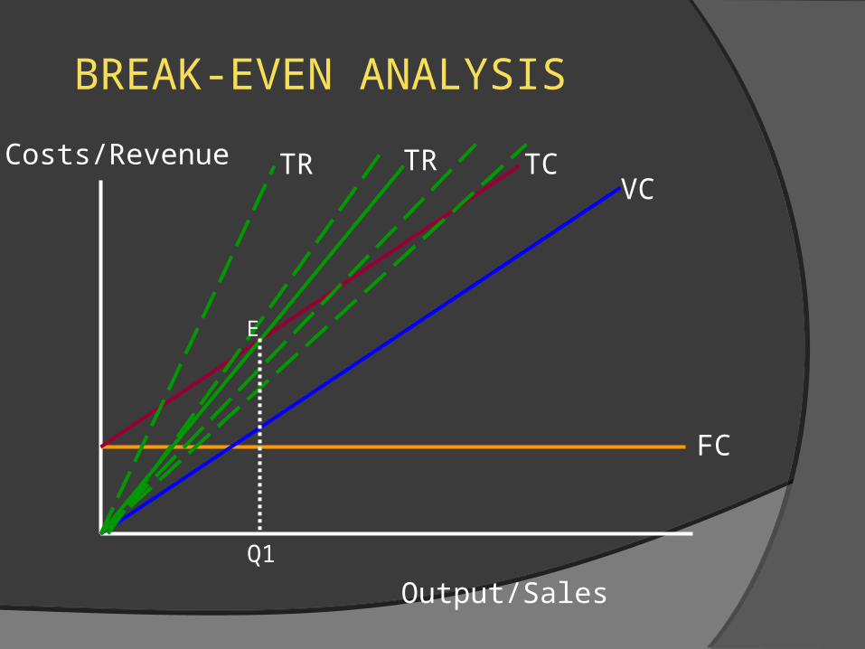
BREAK-EVEN ANALYSIS

Costs/Revenue

Output/Sales

FC

VCTCTR TR

Q1

E

Initially a firm will incur fixed costs, these do not depend on output or sales.

As o/p is generated, the firm will incur variable costs – these vary directly with the amount produced

The total costs therefore (assuming accurate forecasts!) is the sum of FC+VC

Total revenue is determined by the price charged and the quantity sold – again this will be determined by expected forecast sales initially.

The lower the price, the less steep the total revenue curve. The Break-even point occurs where total revenue equals

total costs – the firm, in this example would have to sell Q1 to generate sufficient revenue to cover its costs.

BREAK-EVEN ANALYSIS

• Study of interrelationships among a firm’s sales, costs, and operating profit at various levels of output

• Break-even point is the Q where TR = TC (Q1 to Q2 on graph)

TR

TC

Q

$’s

Profit

Q1 Q2

TC

B2

TOTAL TR

C & R BI

F TFC

0 Q1 Q2

OUTPUT PER TIME UNIT

BEA - NON LINEAR GRAPH

• TFC line shows the fixed cost and the vertical distance between TC and TFC measures the TVC. • The curve TR shows the total sale proceeds or the total revenue (TR) at different levels of o/p and price.• The vertical distance between the TR and TC measures the profit or loss for various levels of output . • TR and TC curves intersect each other at two points, b1 and b2, where TR = TC. these are the lower and upper break-even points. • For the whole range of O/P b/w OQ1 (corresponding to break-even point, b1) an OQ2 (corresponding to break-even point b2), TR>TC. It implies that a firm produces more than OQ1 and less than OQ2 will make profits. In other words, the profitable range of output lies between OQ1 and OQ2 units of output. Producing less or more then these limit will result in losses.

BEP AND PRICING..• Importance of Price Elasticity of Demand:• Higher prices might mean fewer sales to break-

even but those sales may take a longer time to achieve.

• Lower prices might encourage more customers but higher volume needed before sufficient revenue generated to break-even

BEP AND PRICING..

Costs/Revenue

Output/Sales

FC

VCTCTR (p = £2)

Q1

TR (p = £1)

Q3

If the firm chose to set prices lower (say £1) it would need to sell more units before covering its costs

BEP AND PRICING.

Costs/Revenue

Output/Sales

FC

VCTC

TR (p = Rs.2)

Q1

TR (p = Rs.3)

Q2

If the firm chose to set price higher than Rs.2 (say Rs.3) the TR curve would be steeper – they would not have to sell as many units to break even.

BREAK-EVEN ANALYSIS.

Costs/Revenue

Output/Sales

FC

VC

TCTR (p = £2)

Q1

Loss

Profit

BREAK-EVEN ANALYSIS

Links of BE to pricing strategies and elasticity

• Penetration pricing – ‘high’ volume, ‘low’ price – more sales to break even

• Market Skimming – ‘high’ price ‘low’ volumes – fewer sales to break even

• Elasticity – what is likely to happen to sales when prices are increased or decreased?

APPLICATION OF BEA..•The break-even point is one of the simplest yet least used analytical tools in management.

• It helps to provide a dynamic view of the relationships between sales, costs and profits.

• A better understanding of break-even—for example, expressing break-even sales as a percentage of actual sales—can give managers a chance to understand when to expect to break even (by linking the percent to when in the week/month this percent of sales might occur).

•The break-even point is a special case of Target Income Sales, where Target Income is 0 (breaking even).

ASSUMPTION. The cost and revenue function are linear. The total cost is divided into fixed and

variable costs. The selling price is constant. The volume of sales and volume of

production are identical. Average and marginal productivity of

factors are constant. Factor price is constant..

• IT IS STATIC AND UNREALISTIC

• Break-even analysis is only a supply side (i.e. costs only) analysis, as it tells you nothing about what sales are actually likely to be for the product at these various prices.

• It assumes that fixed costs (FC) are constant

•It assumes that the quantity of goods produced is equal to the quantity of goods sold (i.e., there is no change in the quantity of goods held in inventory at the beginning of the period and the quantity of goods held in inventory at the end of the period).

..

ALGEBRAIC SOLUTION.

• Equate total revenue and total cost functions and solve for Q TR = P x Q TC = FC + (VC x Q) TR = TC P x Q = FC + VC x Q Q(P-VC)=FC Q=FC/(P-VC) BREAK EVEN SALES=FC*SALES/(SALES-VC)

EXAMPLE 1 : How many Christmas trees need to be sold ?

• Wholesale price per tree is $8.00• Fixed cost is $30,000• Variable cost per tree is $5.00• Solution

Q(break-even) = FC/(P – VC) = $30,000/($8 - $5)

= $30,000/$3 = 10,000 trees Break even sales are=10000*$8=$80,000

THANK YOU