University of Pennsylvania University of Pennsylvania

ScholarlyCommons ScholarlyCommons

Scholarship at Penn Libraries Penn Libraries

January 1999

Aviation and the Global Atmosphere: A Special Report of IPCC Aviation and the Global Atmosphere: A Special Report of IPCC

Working Groups I and III Working Groups I and III

Anu Vedantham University of Pennsylvania, vedantha@pobox.upenn.edu

Follow this and additional works at: https://repository.upenn.edu/library_papers

Recommended Citation Recommended Citation Vedantham, A. (1999). Aviation and the Global Atmosphere: A Special Report of IPCC Working Groups I and III. Retrieved from https://repository.upenn.edu/library_papers/61

This excerpt from the IPCC publication,Aviation and the Global Atmosphere, includes the summary for policymakers and Chapter 9 "Aircraft Emissions: Current Inventories and Future Scenarios." The complete report is available on the web at http://www.ipcc.ch Wickrama, U.K., Henderson, S.C., Vedantham, A., et al. (1999) Chapter 9 Aircraft Emissions: Current Inventories and Future Scenarios. Aviation and the Global Atmosphere. Intergovernmental Panel on Climate Change. Cambridge: Cambridge University Press

This paper is posted at ScholarlyCommons. https://repository.upenn.edu/library_papers/61 For more information, please contact repository@pobox.upenn.edu.

Aviation and the Global Atmosphere: A Special Report of IPCC Working Groups I Aviation and the Global Atmosphere: A Special Report of IPCC Working Groups I and III and III

Abstract Abstract This report assesses the effects of aircraft on climate and atmospheric ozone and is the first IPCC report for a specific industrial subsector. It was prepared by IPCC in collaboration with the Scientific Assessment Panel to the Montreal Protocol on Substances that Deplete the Ozone Layer, in response to a request by the International Civil Aviation Organization (ICAO) because of the potential impact of aviation emissions. These are the predominant anthropogenic emissions deposited directly into the upper troposphere and lower stratosphere.

Aviation has experienced rapid expansion as the world economy has grown. Passenger traffic (expressed as revenue passenger kilometers) has grown since 1960 at nearly 9% per year, 2.4 times the average Gross Domestic Product (GDP) growth rate. Freight traffic, approximately 80% of which is carried by passenger airplanes, has also grown over the same time period. The rate of growth of passenger traffic has slowed to about 5% in 1997 as the industry is maturing. Total aviation emissions have increased, because increased demand for air transport has outpaced the reductions in specific emissions from the continuing improvements in technology and operational procedures. Passenger traffic, assuming unconstrained demand, is projected to grow at rates in excess of GDP for the period assessed in this report.

Keywords Keywords global warming, aircraft, emissions, chemistry

Comments Comments This excerpt from the IPCC publication,Aviation and the Global Atmosphere, includes the summary for policymakers and Chapter 9 "Aircraft Emissions: Current Inventories and Future Scenarios." The complete report is available on the web at http://www.ipcc.ch Wickrama, U.K., Henderson, S.C., Vedantham, A., et al. (1999) Chapter 9 Aircraft Emissions: Current Inventories and Future Scenarios. Aviation and the Global Atmosphere. Intergovernmental Panel on Climate Change. Cambridge: Cambridge University Press

This government publication is available at ScholarlyCommons: https://repository.upenn.edu/library_papers/61

SUMMARY FOR POLICYMAKERS

AVIATION AND THE GLOBAL ATMOSPHERE

A Special Report ofWorking Groups I and IIIof the Intergovernmental Panel on Climate Change

This summary, approved in detail at a joint session of IPCC Working Groups I and III(San Jose, Costa Rica· 12-14 April 1999), represents the formally agreed statement of the IPCCconcerning current understanding of aviation and the global atmosphere.

Based on a draft prepared by:

David H. Lister, Joyce E. Penner, David J. Griggs, John T. Houghton, Daniel L. Albritton, John Begin, Gerard Bekebrede,John Crayston, Ogunlade Davidson, Richard G. Derwent, David 1. Dokken, Julie Ellis, David W. Fahey, John E. Frederick,Randall Friedl, Neil Harris, Stephen C. Henderson, John F. Hennigan, Ivar Isaksen, Charles H. Jackman, Jerry Lewis,Mack McFarland, Bert Metz, John Montgomery, Richard W. Niedzwiecki, Michael Prather, Keith R. Ryan, Nelson Sabogal,Robert Sausen, Ulrich Schumann, Hugh J. Somerville, N. Sundararaman, Ding Yihui, Upali K. Wickrama, Howard L. Wesoky

--

Aviation and the Global Atmosphere

1. Introduction

This report assesses the effects of aircraft on climate andatmospheric ozone and is the first IPCC report for a specificindustrial subsector. It was prepared by IPCC in collaborationwith the Scientific Assessment Panel to the Montreal Protocolon Substances that Deplete the Ozone Layer, in response to arequest by the International Civil Aviation Organization(ICAO)1 because of the potential impact ofaviation emissions.These are the predominant anthropogenic emissions depositeddirectly into the upper troposphere and lower stratosphere.

Aviation has experienced rapid expansion as the world economyhas grown. Passenger traffic (expressed as revenue passenger­kilometersZ) has grown since 1960 at nearly 9% per year, 2.4times the average Gross Domestic Product (GDP) growth rate.Freight traffic, approximately 80% of which is carried bypassenger airplanes, has also grown over the same time period.The rate ofgrowth ofpassenger traffic has slowed to about 5%in 1997 as the industry is maturing. Total aviation emissionshave increased, because increased demand for air transport hasoutpaced the reductions in specific emissions3 from the continuingimprovements in technology and operational procedures.Passenger traffic, assuming unconstrained demand, is projected togrow at rates in excess of GDP for the period assessed in this report.

The effects of current aviation and of a range of unconstrainedgrowth projections for aviation (which include passenger,freight, and military) are examined in this report, including thepossible effects of a fleet of second generation, commercialsupersonic aircraft. The report also describes current aircrafttechnology, operating procedures, and options for mitigatingaviation's future impact on the global atmosphere. Thereport does not consider the local environmental effects ofaircraft engine emissions or any of the indirect environmentaleffects of aviation operations such as energy usage by groundtransportation at airports.

2. How Do Aircraft Affect Climate and Ozone?

Aircraft emit gases and particles directly into the uppertroposphere and lower stratosphere where they have an impacton atmospheric composition. These gases and particles alterthe concentration of atmospheric greenhouse gases, includingcarbon dioxide (COz), ozone (03), and methane (CH4); triggerformation ofcondensation trails (contrails); and may increasecirrus cloudiness-all of which contribute to climate change(see Box 1).

The principal emISSIOns of aircraft include the greenhousegases carbon dioxide and water vapor (HzO). Other majoremissions are nitric oxide (NO) and nitrogen dioxide (NOz)(which together are termed NOx), sulfur oxides (SOx), and soot.The total amount of aviation fuel burned, as well as the totalemissions of carbon dioxide, NOx, and water vapor by aircraft,are well known relative to other parameters important to thisassessment.

3

The climate impacts of the gases and particles emitted andformed as a result of aviation are more difficult to quantify thanthe emissions; however, they can be compared to each otherand to climate effects from other sectors by using the conceptof radiative forcing.4 Because carbon dioxide has a longatmospheric residence time ('"100 years) and so becomes wellmixed throughout the atmosphere, the effects of its emissionsfrom aircraft are indistinguishable from the same quantity ofcarbon dioxide emitted by any other source. The other gases(e.g., NOx, SOx, water vapor) and particles have shorteratmospheric residence times and remain concentrated nearflight routes, mainly in the northern mid-latitudes. Theseemissions can lead to radiative forcing that is regionally locatednear the flight routes for some components (e.g., ozone andcontrails) in contrast to emissions that are globally mixed (e.g.,carbon dioxide and methane).

The global mean climate change is reasonably well representedby the global average radiative forcing, for example, whenevaluating the contributions of aviation to the rise in globallyaveraged temperature or sea level. However, because someof aviation's key contributions to radiative forcing arelocated mainly in the northern mid-latitudes, the regionalclimate response may differ from that derived from a globalmean radiative forcing. The impact of aircraft on regionalclimate could be important, but has not been assessed in thisreport.

Ozone is a greenhouse gas. It also shields the surface of theearth from harmful ultraviolet (UV) radiation, and is a commonair pollutant. Aircraft-emitted NOx participates in ozonechemistry. Subsonic aircraft fly in the upper troposphere andlower stratosphere (at altitudes of about 9 to 13 km), whereassupersonic aircraft cruise several kilometers higher (at about17 to 20 km) in the stratosphere. Ozone in the upper troposphereand lower stratosphere is expected to increase in response toNOx increases and methane is expected to decrease. At higheraltitudes, increases in NOxlead to decreases in the stratosphericozone layer. Ozone precursor (NOx) residence times in theseregions increase with altitude, and hence perturbations toozone by aircraft depend on the altitude of NOx injection andvary from regional in scale in the troposphere to global in scalein the stratosphere.

1 ICAO is the United Nations specialized agency that has globalresponsibility for the establishment of standards, recommendedpractices, and guidance on various aspects of international civilaviation, including environmental protection.

z The revenue passenger-km is a measure of the traffic carried bycommercial aviation: one revenue-paying passenger carried 1 km.

3 Specific emissions are emissions per unit of traffic carried, forinstance, per revenue passenger-km.

4 Radiative forcing is a measure of the importance of a potentialclimate change mechanism. It expresses the perturbation or changeto the energy balance of the Earth-atmosphere system in watts persquare meter (Wm-2). Positive values of radiative forcing imply anet warming, while negative values imply cooling.

Aviation and the Global Atmosphere 5

Table 1: Summary offuture global aircraft scenarios used in this report.

Avg.1hd1ic Avg.Annuai Avg.Annuai Avg.AnnuaiGrowth Growth Rate Economic Population Ratio of Ratio of

Scenario per Year ofFuel Burn Growth Growth Traffic Fuel BurnName (1990-2050)1 (1990-2050)2 Rate Rate (2050/1990) (2050/1990) Notes

Fal 3.1% 1.7% 2.9% 1.4% 6.4 2.7 Reference scenario developed by1990-2025 1990-2025 ICAO Forecasting and Economic

2.3% 0.7% Support Group (FESG); mid-range1990-2100 1990-2100 economic growth from IPCC

(1992); technology for bothimproved fuel efficiency and NOx

reduction

FalH 3.1 % 2.0% 2.9% 1.4% 6.4 3.3 Fal traffic and technology scenario1990-2025 1990-2025 with a fleet of supersonic aircraft

2.3% 0.7% replacing some of the subsonic1990-2100 1990-2100 fleet

Fa2 3.1% 1.7% 2.9% 1.4% 6.4 2.7 Fal traffic scenario; technology1990-2025 1990-2025 with greater emphasis on NOx

2.3% 0.7% reduction, but slightly smaller fuel1990-2100 1990-2100 efficiency improvement

Fcl 2.2% 0.8% 2.0% 1.1% 3.6 1.6 FESG low-growth scenario;1990-2025 1990-2025 technology as for Fal scenario

1.2% 0.2%1990-2100 1990-2100

Fel 3.9% 2.5% 3.5% 1.4% 10.1 4.4 FESG high-growth scenario;1990-2025 1990-2025 technology as for Fal scenario

3.0% 0.7%1990-2100 1990-2100

Eab

Edh

4.0%

4.7%

3.2%

3.8%

10.7

15.5

6.6

9.4

Traffic-growth scenario based onIS92a developed by EnvironmentalDefense Fund (EDF); technologyfor very low NOx assumed

High traffic-growth EDF scenario;technology for very low NOx

assumed

ITraffic measured in terms of revenue passenger-km.2All aviation (passenger, freight, and military).

ideal air traffic management) is achieved by 2050. If theseimprovements do not materialize then fuel use and emissionswill be higher. It is further assumed that the number of aircraftas well as the number of airports and associated infrastructurewill continue to grow and not limit the growth in demand forair travel. If the infrastructure was not available, the growth oftraffic reflected in these scenarios would not materialize.

IPCC (1992)7 developed a range of scenarios, IS92a-f, offuture greenhouse gas and aerosol precursor emissions basedon assumptions concerning population and economic growth,

land use, technological changes, energy availability, and fuelmix during the period 1990 to 2100. Scenario IS92a is a mid­range emissions scenario. Scenarios of future emissions are notpredictions of the future. They are inherently uncertain becausethey are based on different assumptions about the future, and

7 IPCC, 1992: Climate Change 1992: The Supplementary Report tothe IPCC Scientific Assessment [Houghton, LT., B.A. Callander,and S.K.Varney (eds.)]. Cambridge University Press, Cambridge,UK, 200 pp.

6

the longer the time horizon the more uncertain these scenariosbecome. The aircraft emissions scenarios developed here usedthe economic growth and population assumptions found in theIS92 scenario range (see Table 1 and Figure 1). In the followingsections, scenario Fa1 is utilized to illustrate the possibleeffects of aircraft and is called the reference scenario. Itsassumptions are linked to those of IS92a. The other aircraftemissions scenarios were built from a range of economic andpopulation projections from IS92a-e. These scenarios representa range of plausible growth for aviation and provide a basis forsensitivity analysis for climate modeling. However, the highgrowth scenario Edh is believed to be less plausible and thelow growth scenario Fc1 is likely to be exceeded given thepresent state of the industry and planned developments.

4. What are the Current and Future Impactsof Subsonic Aviation on Radiative Forcingand UV Radiation?

The summary of radiative effects resulting from aircraft engineemissions is given in Figures 2 and 3. As shown in Figure 2,the uncertainty associated with several of these effects is large.

4.1. Carbon Dioxide

Emissions ofcarbon dioxide by aircraft were 0.14 Gt C/year in1992. This is about 2% of total anthropogenic carbon dioxideemissions in 1992 or about 13% of carbon dioxide emissionsfrom all transportation sources. The range ofscenarios consideredhere projects that aircraft emissions of carbon dioxide willcontinue to grow and by 2050 will be 0.23 to 1045 Gt C/year.For the reference scenario (Fal) this emission increases 3-fold

1.6;:::' Edh 900 ....r.. 1.4

/ 800 =~ ""U 1.2 / 700'"l~.... III

/ 600 rnS2, 1.0 Eab ~

/" rnrn / 500 5'= 0.8 /.~ / 400 ""/" Fe! ~

rn 0.6 / /" - 300 .....;!l/" _ - FalH Ie>

~Ie>

0.4 ./ ~ -_-::::---- 200 ~

'" -- Fal 100 ,-..0 0.2 - - - - - . - . - - <f1.u Fe! 0 '-'

0.01990 2000 2010 2020 2030 2040 2050

Year

Figure 1: Total aviation carbon dioxide emissions resultingfrom six different scenarios for aircraft fuel use. Emissionsare given in Gt C [or billion (109) tonnes of carbon] per year.To convert Gt C to Gt CO2 multiply by 3.67. The scale on therighthand axis represents the percentage growth from 1990 to2050. Aircraft emissions of carbon dioxide represent 2.4% oftotal fossil fuel emissions of carbon dioxide in 1992 or 2% oftotal anthropogenic carbon dioxide emissions. (Note: Fa2 hasnot been drawn because the difference from scenario Fa1would not be discernible on the figure.)

Aviation and the Global Atmosphere

by 2050 to 0040 Gt C/year, or 3% of the projected totalanthropogenic carbon dioxide emissions relative to the mid­range 1PCC emission scenario (lS92a). For the range ofscenarios, the range of increase in carbon dioxide emissions to2050 would be 1.6 to 10 times the value in 1992.

Concentrations of and radiative forcing from carbon dioxidetoday are those resulting from emissions during the last 100 yearsor so. The carbon dioxide concentration attributable to aviation inthe 1992 atmosphere is 1 ppmv, a little more than 1% of the totalanthropogenic increase. This percentage is lower than thepercentage for emissions (2%) because the emissions occurredonly in the last 50 years. For the range of scenarios in Figure 1,the accumulation of atmospheric carbon dioxide due to aircraftover the next 50 years is projected to increase to 5 to 13 ppmv.For the reference scenario (Fa1) this is 4% of that from all humanactivities assuming the mid-range IPCC scenario (IS92a).

42. Ozone

The NOx emissions from subsonic aircraft in 1992 are estimatedto have increased ozone concentrations at cruise altitudes innorthern mid-latitudes by up to 6%, compared to an atmospherewithout aircraft emissions. This ozone increase is projected torise to about 13% by 2050 in the reference scenario (Fal). Theimpact on ozone concentrations in other regions of the world issubstantially less. These increases will, on average, tend towarm the surface of the Earth.

Aircraft emissions of NOx are more effective at producingozone in the upper troposphere than an equivalent amount ofemission at the surface. Also increases in ozone in the uppertroposphere are more effective at increasing radiative forcingthan increases at lower altitudes. Due to these increases thecalculated total ozone column in northern mid-latitudes isprojected to grow by approximately 0.4 and 1.2% in 1992 and2050, respectively. However, aircraft sulfur and water emissionsin the stratosphere tend to deplete ozone, partially offsettingthe NOx-induced ozone increases. The degree to which thisoccurs is, as yet, not quantified. Therefore, the impact ofsubsonic aircraft emissions on stratospheric ozone requiresfurther evaluation. The largest increases in ozone concentrationdue to aircraft emissions are calculated to occur near thetropopause where natural variability is high. Such changes arenot apparent from observations at this time.

4.3. Methane

In addition to increasing tropospheric ozone concentrations,aircraft NOx emissions are expected to decrease the concentrationof methane, which is also a greenhouse gas. These reductionsin methane tend to cool the surface of the Earth. The methaneconcentration in 1992 is estimated here to be about 2% lessthan that in an atmosphere without aircraft. This aircraft­induced reduction of methane concentration is much smallerthan the observed overall 2.5-fold increase since pre-industrial

Figure 2: Estimates of the globally and annually averagedradiative forcing (Wm-2) (see Footnote 4) from subsonicaircraft emissions in 1992 (2a) and in 2050 for scenario Fal(2b). The scale in Figure 2b is greater than the scale in 2a byabout a factor of 4. The bars indicate the best estimate offorcing while the line associated with each bar is a two-thirdsuncertainty range developed using the best knowledge andtools available at the present time. (The two-thirds uncertaintyrange means that there is a 67% probability that the truevalue falls within this range.) The available information oncirrus clouds is insufficient to determine either a best estimateor an uncertainty range; the dashed line indicates a range ofpossible best estimates. The estimate for total forcing doesnot include the effect of changes in cirrus cloudiness. Theuncertainty estimate for the total radiative forcing (withoutadditional cirrus) is calculated as the square root of the sumsof the squares of the upper and lower ranges for the individualcomponents. The evaluations below the graph ("good,""fair," "poor," "very poor") are a relative appraisal associatedwith each component and indicates the level of scientificunderstanding. It is based on the amount of evidence availableto support the best estimate and its uncertainty, the degree ofconsensus in the scientific literature, and the scope of theanalysis. This evaluation is separate from the evaluation ofuncertainty range represented by the lines associated witheach bar. This method of presentation is different and moremeaningful than the confidence level presented in similargraphs from Climate Change 1995: The Science of ClimateChange.

4.5. Contrails

7

within I to 2 weeks. A smallerfraction ofwater vapor emissionsis released in the lower stratosphere where it can build up tolarger concentrations. Because water vapor is a greenhousegas, these increases tend to warm the Earth's surface, thoughfor subsonic aircraft this effect is smaller than those of otheraircraft emissions such as carbon dioxide and NOx '

In 1992, aircraft line-shaped contrails are estimated to coverabout O.I% of the Earth's surface on an annually averagedbasis with larger regional values. Contrails tend to warm theEarth's surface, similar to thin high clouds. The contrail coveris projected to grow to 0.5% by 2050 in the reference scenario(FaI), at a rate which is faster than the rate ofgrowth in aviationfuel consumption. This faster growth in contrail cover isexpected because air traffic will increase mainly in the uppertroposphere where contrails form preferentially, and may alsooccur as a result of improvements in aircraft fuel efficiency.Contrails are triggered from the water vapor emitted by aircraftand their optical properties depend on the particles emitted orformed in the aircraft plume and on the ambient atmosphericconditions. The radiative effect of contrails depends on theiroptical properties and global cover, both of which are uncertain.Contrails have been observed as line-shaped clouds by satellites

Direct TotalSoot (without

cirrusclouds)

Direct TotalSoot (without

cirrusclouds)

DirectSulfate

1-.....~Contrails ci~~ .su~ate

Clouds

ICH4 ~

03._.~ Contrails c:;~· I1 Clouds

~fromNOx

Radiative Forcing from Aircraft in 2050

good fair poor poor fair very fair fairpoor

CO2

Radiative Forcing from Aircraft in 1992

a)

good poor poor poor fair very fair fairpoor

0.10..--------------------:=---,

-0.2

~================:;-----'

-0.1

0.08

-0.06

~e 0.06

~tlJI 0.04

=.~ 0.02~QI

~ 0.00

i -0.02~

-0.04

Aviation and the Global Atmosphere

0.5 b)

Changes in tropospheric ozone are mainly in the NorthernHemisphere, while those of methane are global in extent sothat, even though the global average radiative forcings are ofsimilar magnitude and opposite in sign, the latitudinal structureof the forcing is different so that the net regional radiativeeffects do not cancel.

times. Uncertainties in the sources and sinks of methanepreclude testing the impact of aviation on methane concentrationswith atmospheric observations. In the reference scenario (FaI)methane would be about 5% less than that calculated for a2050 atmosphere without aircraft.

Most subsonic aircraft water vapor emissions are released inthe troposphere where they are rapidly removed by precipitation

4.4. Water Vapor

0.4

i OJ'-'tlJI.5 0.2l::o~QI 0.1

~~ 0.0

8

over heavy air traffic areas and covered on average about 0.5%of the area over Central Europe in 1996 and 1997.

4.6. Cirrus Clouds

Extensive cirrus clouds have been observed to develop afterthe formation ofpersistent contrails. Increases in cirrus cloudcover (beyond those identified as line-shaped contrails) arefound to be positively correlated with aircraft emissions in alimited number of studies. About 30% of the Earth is coveredwith cirrus cloud. On average an increase in cirrus cloud covertends to warm the surface ofthe Earth. An estimate for aircraft­induced cirrus cover for the late I990s ranges from 0 to 0.2%of the surface of the Earth. For the FaI scenario, this maypossibly increase by a factor of4 (0 to 0.8%) by 2050; however,the mechanisms associated with increases in cirrus cover arenot well understood and need further investigation.

4.7. Sulfate and Soot Aerosols

The aerosol mass concentrations in 1992 resulting from aircraftare small relative to those caused by surface sources. Althoughaerosol accumulation will grow with aviation fuel use, aerosolmass concentrations from aircraft in 2050 are projected toremain small compared to surface sources. Increases in soottend to warm while increases in sulfate tend to cool the Earth'ssurface. The direct radiative forcing of sulfate and soot aerosolsfrom aircraft is small compared to those of other aircraftemissions. Because aerosols influence the formation of clouds,the accumulation of aerosols from aircraft may play a role inenhanced cloud formation and change the radiative propertiesof clouds.

4.8. What are the Overall Climate Effectsof Subsonic Aircraft?

The climate impacts of different anthropogenic emissions canbe compared using the concept of radiative forcing. The bestestimate ofthe radiative forcing in 1992 by aircraft is 0.05 Wm-2

or about 3.5% ofthe total radiative forcing by all anthropogenicactivities. For the reference scenario (FaI ), the radiative forcingby aircraft in 2050 is O.I9 Wm- 2 or 5% of the radiative forcingin the mid-range IS92a scenario (3.8 times the value in 1992).According to the range ofscenarios considered here, the forcingis projected to grow to 0.13 to 0.56 Wm-2 in 2050, which is afactor of 1.5 less to a factor of3 greater than that for FaI andfrom 2.6 to II times the value in 1992. These estimates of forcingcombine the effects from changes in concentrations of carbondioxide, ozone, methane, water vapor, line-shaped contrails, andaerosols, but do not include possible changes in cirrus clouds.

Globally averaged values of the radiative forcing from differentcomponents in 1992 and in 2050 under the reference scenario(Fal) are shown in Figure 2. Figure 2 indicates the bestestimates of the forcing for each component and the two-thirds

Aviation and the Global Atmosphere

uncertainty range.8 The derivation of these uncertainty rangesinvolves expert scientific judgment and may also includeobjective statistical models. The uncertainty range in the radiativeforcing stated here combines the uncertainty in calculating theatmospheric change to greenhouse gases and aerosols with thatof calculating radiative forcing. For additional cirrus clouds,only a range for the best estimate is given; this is not includedin the total radiative forcing.

The state of scientific understanding is evaluated for eachcomponent. This is not the same as the confidence level expressedin previous IPCC documents. This evaluation is separate fromthe uncertainty range and is a relative appraisal of the scientificunderstanding for each component. The evaluation is based onthe amount of evidence available to support the best estimateand its uncertainty, the degree of consensus in the scientificliterature, and the scope of the analysis. The total radiativeforcing under each of the six scenarios for the growth of aviationis shown in Figure 3 for the period 1990 to 2050.

The total radiative forcing due to aviation (without forcingfrom additional cirrus) is likely to lie within the range from0.01 to 0.1 Wm-2 in 1992, with the largest uncertainties corningfrom contrails and methane. Hence the total radiative forcingmay be about 2 times larger or 5 times smaller than the bestestimate. For any scenario at 2050, the uncertainty range ofradiative forcing is slightly larger than for 1992, but the largestvariations of projected radiative forcing come from the rangeof scenarios.

Over the period from 1992 to 2050, the overall radiativeforcing by aircraft (excluding that from changes in cirrusclouds) for all scenarios in this report is a factor of 2 to 4 larger

0.6

----Edh.

M

/"8 0.5~ ,/''-'OIl 0.4 /" Eab

= ,/' /''0'" 0.3 /" /'/FalH0~ /' -----ell

,/' /' *",,-, __Fel

.:: 0.2 ......::: ~- -.... ./ ~';;;,-t'" Falell-'-:a --- -

ell 0.1 ~Fc1

~ -01990 2000 2010 2020 2030 2040 2050

Year

Figure 3: Estimates of the globally and annually averagedtotal radiative forcing (without cirrus clouds) associated withaviation emissions under each of six scenarios for the growthof aviation over the time period 1990 to 2050. (Fa2 has notbeen drawn because the difference from scenario Fal wouldnot be discernible on the figure.)

8 The two-thirds uncertainty range means there is a 67% probabilitythat the true value falls within this range.

Aviation and the Global Atmosphere

than the forcing by aircraft carbon dioxide alone. The overall 5.radiative forcing for the sum of all human activities is estimatedto be at most a factor of 1.5 larger than that of carbon dioxide alone.

What are the Current and Future Impactsof Supersonic Aviation on Radiative Forcingand UV Radiation?

9

The emissions of NOx cause changes in methane and ozone,with influence on radiative forcing estimated to be of similarmagnitude but of opposite sign. However, as noted above, thegeographical distribution of the aircraft ozone forcing is farmore regional than that of the aircraft methane forcing.

The effect of aircraft on climate is superimposed on that causedby other anthropogenic emissions of greenhouse gases andparticles, and on the background natural variability. The radiativeforcing from aviation is about 3.5% of the total radiative forcingin 1992. It has not been possible to separate the influence onglobal climate change of aviation (or any other sector withsimilar radiative forcing) from all other anthropogenic activities.Aircraft contribute to global change approximately in proportionto their contribution to radiative forcing.

4.9. What are the Overall EffectsofSubsonic Aircraft on UV-B?

Ozone, most of which resides in the stratosphere, provides ashield against solar ultraviolet radiation. The erythemal doserate, defined as UV irradiance weighted according to howeffectively it causes sunburn, is estimated to be decreased byaircraft in 1992 by about 0.5% at 45oN in July. For comparison,the calculated increase in the erythemal dose rate due toobserved ozone depletion is about 4% over the period 1970 to1992 at 45°N in July.9 The net effect of subsonic aircraftappears to be an increase in column ozone and a decrease inUV radiation, which is mainly due to aircraft NOx emissions.Much smaller changes in UV radiation are associated withaircraft contrails, aerosols, and induced cloudiness. In theSouthern Hemisphere, the calculated effects of aircraft emissionon the erythemal dose rate are about a factor of 4 lower than forthe Northern Hemisphere.

For the reference scenario (Fa1), the change in erythemal doserate at 45 oN in July in 2050 compared to a simulation with noaircraft is -1.3% (with a two-thirds uncertainty range from-0.7 to -2.6%). For comparison, the calculated change in theerythemal dose rate due to changes in the concentrations oftrace species, other than those from aircraft, between 1970 to2050 at 45°N is about -3%, a decrease that is the net result oftwo opposing effects: (1) the incomplete recovery of stratosphericozone to 1970 levels because of the persistence of long-livedhalogen-containing compounds, and (2) increases in projectedsurface emissions of shorter lived pollutants that produce ozonein the troposphere.

9 This value is based on satellite observations and model calculations.See WMO, 1999: Scientific Assessment of Ozone Depletion: 1998.Report No. 44, Global Ozone Research and Monitoring Project,World Meteorological Organization, Geneva, Switzerland, 732 pp.

One possibility for the future is the development of a fleet ofsecond generation supersonic, high speed civil transport(HSCT) aircraft, although there is considerable uncertaintywhether any such fleet will be developed. These supersonicaircraft are projected to cruise at an altitude of about 19 km,about 8 km higher than subsonic aircraft, and to emit carbondioxide, water vapor, NOv SOx, and soot into the stratosphere.NOx, water vapor, and SOx from supersonic aircraft emissionsall contribute to changes in stratospheric ozone. The radiativeforcing of civil supersonic aircraft is estimated to be about afactor of 5 larger than that of the displaced subsonic aircraftin the Fa1H scenario. The calculated radiative forcing ofsupersonic aircraft depends on the treatment of water vaporand ozone in models. This effect is difficult to simulate incurrent models and so is highly uncertain.

Scenario Fa1H considers the addition of a fleet of civilsupersonic aircraft that was assumed to begin operation in theyear 2015 and grow to a maximum of 1,000 aircraft by the year2040. For reference, the civil subsonic fleet at the end of theyear 1997 contained approximately 12,000 aircraft. In thisscenario, the aircraft are designed to cruise at Mach 2.4, andnew technologies are assumed that maintain emissions of 5 gNOz per kg fuel (lower than today's civil supersonic aircraftwhich has emissions of about 22 g NOz per kg fuel). Thesesupersonic aircraft are assumed to replace part of the subsonicfleet (11 %, in terms of emissions in scenario Fa1). Supersonicaircraft consume more than twice the fuel per passenger-kmcompared to subsonic aircraft. By the year 2050, the combinedfleet (scenario Fa1H) is projected to add a further 0.08 Wm-2

(42%) to the 0.19 Wm- 2 radiative forcing from scenarioFa1 (see Figure 4). Most of this additional forcing is due toaccumulation of stratospheric water vapor.

The effect of introducing a civil supersonic fleet to form thecombined fleet (Fa1H) is also to reduce stratospheric ozoneand increase erythemal dose rate. The maximum calculatedeffect is at 45°N where, in July, the ozone column change in2050 from the combined subsonic and supersonic fleet relativeto no aircraft is -0.4%. The effect on the ozone column of thesupersonic component by itself is -1.3% while the subsoniccomponent is +0.9%.

The combined fleet would change the erythemal dose rate at45°N in July by +0.3% compared to the 2050 atmospherewithout aircraft. The two-thirds uncertainty range for thecombined fleet is -1.7% to +3.3%. This may be compared tothe projected change of -1.3% for Fa1. Flying higher leads tolarger ozone column decreases, while flying lower leads tosmaller ozone column decreases and may even result in anozone column increase for flight in the lowermost stratosphere.In addition, emissions from supersonic aircraft in the NorthernHemisphere stratosphere may be transported to the SouthernHemisphere where they cause ozone depletion.

10 Aviation and the Global Atmosphere

Radiative Forcing from Aircraft in 2050with Supersonic Fleet

0.6• Supersonic Fleet

,-. 0.5Subsonic Fleet'"e 0.4 • Combined Fleet

~gf 0.3

-20.20....

~ 0.1

I~:.= ICH4eo=

:a 0 - ....~ -,"

eo= CO2 I~ -0.10 3

"-v-J-0.2 fromNOx

tIlContrails Cirrus

Clouds

DirectSulfate

:J:Direct TotalSoot (without

cirrusclouds)

affect the introduction ofimprovements and may affect demandfor air transport. Mitigation options for water vapor andcloudiness have not been fully addressed.

Safety of operation, operational and environmental performance,and costs are dominant considerations for the aviation industrywhen assessing any new aircraft purchase or potentialengineering or operational changes. The typical life expectancyof an aircraft is 25 to 35 years. These factors have to be takeninto account when assessing the rate at which technologyadvances and policy options related to technology can reduceaviation emissions.

6.1. Aircraft and Engine Technology Options

Figure 4: Estimates of the globally and annually averagedradiative forcing from a combined fleet of subsonic andsupersonic aircraft (in Wm-2) due to changes in greenhousegases, aerosols, and contrails in 2050 under the scenarioFaIR. In this scenario, the supersonic aircraft are assumed toreplace part of the subsonic fleet (11 %, in terms of emissionsin scenario Fal). The bars indicate the best estimate of forcingwhile the line associated with each bar is a two-thirdsuncertainty range developed using the best knowledge andtools available at the present time. (The two-thirds uncertaintyrange means that there is a 67% probability that the truevalue falls within this range.) The available information oncirrus clouds is insufficient to determine either a best estimateor an uncertainty range; the dashed line indicates a range ofpossible best estimates. The estimate for total forcing doesnot include the effect of changes in cirrus cloudiness. Theuncertainty estimate for the total radiative forcing (withoutadditional cirrus) is calculated as the square root of the sumsof the squares of the upper and lower ranges. The level ofscientific understanding for the supersonic components arecarbon dioxide, "good;" ozone, "poor;" and water vapor, "poor."

6. What are the Optionsto Reduce Emissions and Impacts?

There is a range of options to reduce the impact of aviationemissions, including changes in aircraft and engine technology,fuel, operational practices, and regulatory and economicmeasures. These could be implemented either singly or incombination by the public and/or private sector. Substantialaircraft and engine technology advances and the air trafficmanagement improvements described in this report are alreadyincorporated in the aircraft emissions scenarios used forclimate change calculations. Other operational measures,which have the potential to reduce emissions, and alternativefuels were not assumed in the scenarios. Further technologyadvances have the potential to provide additional fuel andemissions reductions. In practice, some of the improvementsare expected to take place for commercial reasons. The timingand scope of regulatory, economic, and other options may

Technology advances have substantially reduced most emissionsper passenger-km. However, there is potential for furtherimprovements. Any technological change may involve a balanceamong a range of environmental impacts.

Subsonic aircraft being produced today are about 70% morefuel efficient per passenger-km than 40 years ago. The majorityof this gain has been achieved through engine improvementsand the remainder from airframe design improvement. A 20%improvement in fuel efficiency is projected by 2015 and a 40to 50% improvement by 2050 relative to aircraft producedtoday. The 2050 scenarios developed for this report alreadyincorporate these fuel efficiency gains when estimating fueluse and emissions. Engine efficiency improvements reduce thespecific fuel consumption and most types of emissions;however, contrails may increase and, without advances incombuster technology, NOx emissions may also increase.

Future engine and airframe design involves a complex decision­making process and a balance of considerations among manyfactors (e.g., carbon dioxide emissions, NOx emissions atground level, NOx emissions at altitude, water vapor emissions,contrail/cirrus production, and noise). These aspects have notbeen adequately characterized or quantified in this report.

Internationally, substantial engine research programs are inprogress, with goals to reduce Landing and Take-off cycle (LTO)emissions of NOx by up to 70% from today's regulatory standards,while also improving engine fuel consumption by 8 to 10%,over the most recently produced engines, by about 2010.Reduction of NOx emissions would also be achieved at cruisealtitude, though not necessarily by the same proportion as forLTO. Assuming that the goals can be achieved, the transfer ofthis technology to significant numbers of newly produced aircraftwill take longer-typically a decade. Research programs addressingNOx emissions from supersonic aircraft are also in progress.

6.2. Fuel Options

There would not appear to be any practical alternatives tokerosene-based fuels for commercial jet aircraft for the next

Aviation and the Global Atmosphere

several decades. Reducing sulfur content of kerosene willreduce SOx emissions and sulfate particle formation.

Jet aircraft require fuel with a high energy density, especiallyfor long-haul flights. Other fuel options, such as hydrogen,may be viable in the long term, but would require new aircraftdesigns and new infrastructure for supply. Hydrogen fuelwould eliminate emissions of carbon dioxide from aircraft, butwould increase those of water vapor. The overall environmentalimpacts and the environmental sustainability of the productionand use of hydrogen or any other alternative fuels have notbeen determined.

The formation of sulfate particles from aircraft emISSIons,which depends on engine and plume characteristics, is reducedas fuel sulfur content decreases. While technology exists toremove virtually all sulfur from fuel, its removal results in areduction in lubricity.

6.3. Operational Options

Improvements in air traffic management (ATM) and otheroperational procedures could reduce aviation fuel burn bybetween 8 and 18%. The large majority (6 to 12%) of thesereductions comes from ATM improvements which it is anticipatedwill be fully implemented in the next 20 years. All engineemissions will be reduced as a consequence. In all aviationemission scenarios considered in this report the reductionsfrom ATM improvements have already been taken into account.The rate of introduction of improved ATM will depend on theimplementation of the essential institutional arrangements atan international level.

Air traffic management systems are used for the guidance,separation, coordination, and control of aircraft movements.Existing national and international air traffic managementsystems have limitations which result, for example, in holding(aircraft flying in a fixed pattern waiting for permission toland), inefficient routings, and sub-optimal flight profiles.These limitations result in excess fuel bum and consequentlyexcess emissions.

For the current aircraft fleet and operations, addressing theabove-mentioned limitations in air traffic management systemscould reduce fuel burned in the range of 6 to 12%. It is anticipatedthat the improvement needed for these fuel bum reductionswill be fully implemented in the next 20 years, provided thatthe necessary institutional and regulatory arrangements havebeen put in place in time. The scenarios developed in thisreport assume the timely implementation of these ATMimprovements, when estimating fuel use.

Other operational measures to reduce the amount of fuelburned per passenger-km include increasing load factors(carrying more passengers or freight on a given aircraft),eliminating non-essential weight, optimizing aircraft speed,limiting the use of auxiliary power (e.g., for heating, ventilation),

11

and reducing taxiing. The potential improvements in theseoperational measures could reduce fuel burned, and emissions,in the range 2 to 6%.

Improved operational efficiency may result in attractingadditional air traffic, although no studies providing evidenceon the existence of this effect have been identified.

6.4. Regulatory, Economic, and Other Options

Although improvements in aircraft and engine technology and inthe efficiency of the air traffic system will bring environmentalbenefits, these will not fully offset the effects of the increasedemissions resulting from the projected growth in aviation. Policyoptions to reduce emissions further include more stringentaircraft engine emissions regulations, removal of subsidies andincentives that have negative environmental consequences,market-based options such as environmental levies (charges andtaxes) and emissions trading, voluntary agreements, researchprograms, and substitution of aviation by rail and coach. Mostof these options would lead to increased airline costs and fares.Some of these approaches have not been fully investigated ortested in aviation and their outcomes are uncertain.

Engine emissions certification is a means for reducing specificemissions. The aviation authorities currently use this approachto regulate emissions for carbon monoxide, hydrocarbons,NOx, and smoke. The International Civil Aviation Organizationhas begun work to assess the need for standards for aircraftemissions at cruise altitude to complement existing LTOstandards for NOx and other emissions.

Market-based options, such as environmental levies (chargesand taxes) and emissions trading, have the potential to encouragetechnological innovation and to improve efficiency, and mayreduce demand for air travel. Many of these approaches havenot been fully investigated or tested in aviation and theiroutcomes are uncertain.

Environmental levies (charges and taxes) could be a means forreducing growth of aircraft emissions by further stimulatingthe development and use of more efficient aircraft and byreducing growth in demand for aviation transportation. Studiesshow that to be environmentally effective, levies would need tobe addressed in an international framework.

Another approach that could be considered for mitigating aviationemissions is emissions trading, a market-based approach whichenables participants to cooperatively minimize the costs of reducingemissions. Emissions trading has not been tested in aviationthough it has been used for sulfur dioxide (S02) in the UnitedStates of America and is possible for ozone-depleting substancesin the Montreal Protocol. This approach is one of the provisionsof the Kyoto Protocol where it applies to Annex B Parties.

Voluntary agreements are also currently being explored as ameans of achieving reductions in emissions from the aviation

12

sector. Such agreements have been used in other sectors toreduce greenhouse gas emissions or to enhance sinks.

Measures that can also be considered are removal of subsidiesor incentives which would have negative environmentalconsequences, and research programs.

Substitution by rail and coach could result in the reduction ofcarbon dioxide emissions per passenger-km. The scope for thisreduction is limited to high density, short-haul routes, whichcould have coach or rail links. Estimates show that up to 10%of the travelers in Europe could be transferred from aircraft tohigh-speed trains. Further analysis, including trade-offsbetween a wide range of environmental effects (e.g., noiseexposure, local air quality, and global atmospheric effects) isneeded to explore the potential of substitution.

7. Issues for the Future

This report has assessed the potential climate and ozonechanges due to aircraft to the year 2050 under differentscenarios. It recognizes that the effects ofsome types ofaircraftemissions are well understood. It also reveals that the effects ofothers are not, because of the many scientific uncertainties.There has been a steady improvement in characterizing thepotential impacts of human activities, including the effects ofaviation on the global atmosphere. The report has also examinedtechnological advances, infrastructure improvements, andregulatory or market-based measures to reduce aviationemissions. Further work is required to reduce scientific andother uncertainties, to understand better the options for reducingemissions, to better inform decisionmakers, and to improve theunderstanding of the social and economic issues associatedwith the demand for air transport.

Aviation and the Global Atmosphere

There are a number of key areas of scientific uncertainty thatlimit our ability to project aviation impacts on climate andozone:

• The influence of contrails and aerosols on cirrus clouds• The role of NOx in changing ozone and methane

concentrations• The ability of aerosols to alter chemical processes• The transport of atmospheric gases and particles in the

upper troposphere/lower stratosphere• The climate response to regional forcings and stratospheric

perturbations.

There are a number of key socio-economic and technologicalissues that need greater definition, including inter alia thefollowing:

• Characterization of demand for commercial aVIatlOnservices, including airport and airway infrastructureconstraints and associated technological change

• Methods to assess external costs and the environmentalbenefits of regulatory and market-based optionsAssessment of the macroeconomic effects of emissionreductions in the aviation industry that might resultfrom mitigation measures

• Technological capabilities and operational practices toreduce emissions leading to the formation of contrailsand increased cloudiness

• The understanding of the economic and environmentaleffects of meeting potential stabilization scenarios (foratmospheric concentrations of greenhouse gases), includingmeasures to reduce emissions from aviation and alsoincluding such issues as the relative environmentalimpacts of different transportation modes.

Penn Libraries

Scholarship at Penn Libraries

University of Pennsylvania Year

Aircraft Emissions: Current Inventories

and Future ScenariosS. L. BaughcumJ. J. BeginF. FrancoD. L. GreeneD. S. LeeM.-L. McLarenA. K. MortlockP. J. NewtonA. SchmittD. J. SutkusAnu Vedantham, University of PennsylvaniaD. J. Wuebbles

Reprinted from Aviation and the Global Atmosphere, Intergovernmental Panel on Cli-mate Change, J.E. Penner, D.H. Lister, D.J. Griggs, et al. (eds) (Cambridge: CambridgeUniversity Press, 1999), pages 290-331.

NOTE: At the time of publication, the author Anu Vedantham was affiliated with theU.S. Department of Commerce. Currently, she is a staff member of the UPenn Libraries atthe University of Pennsylvania.

This paper is posted at ScholarlyCommons@Penn.

http://repository.upenn.edu/library papers/59

Review Editor:

O. Davidson

Contributors:

R.M. Gardner, L. Meisenheimer

Lead Authors:

SL. Baughcum, J.J. Begin, F. Franco, DL. Greene, D.S. Lee, M.-L. McLaren,A.K. Mortlock, P.J. Newton, A. Schmitt, D.J. Sutkus, A. Vedantham, D.J. Wuebbles

9

Aircraft Emissions: Current Inventoriesand Future Scenarios

it

! STEPHEN C. HENDERSON AND UPALI K. WICKRAMA

II

Ir

I

CONTENTS

Executive Summary 293 9.5. High-Speed Civil Transport (HSCT) Scenarios 3189.5.1. Description of Methods 319

! 9.1. Introduction 295 9.5.2. Description of Results 320

, 9.2. Factors Affecting Aircraft Emissions 296 9.6. Evaluation and Assessment

9.2.1. Demand for Air Travel 296 of Long-Term Subsonic Scenarios 320

I9.2.2. Developments in Technology 297 9.6.1. Difficulties in Constructing

Long-Term Scenarios 320, 9.3. Historical, Present-Day, and 2015 9.6.2. Structure and Assumptions 321Forecast Emissions Inventories 298 9.6.3. Traffic Demand 3239.3.1. NASA, ANCATIEC2, and DLR Historical 9.6.4. NOx Technology Projections 325

and Present-Day Emissions Inventories 299 9.6.5. Infrastructure and9.3.2. NASA, ANCATJEC2, and DLR Fuel Availability Assumptions 326

2015 Emissions Forecasts 300 9.6.6. Plausibility Checks 3269.3.3. Other Emissions Inventories 302 9.6.6.1. Fleet Size 3269.3.4. Comparisons of Present-Day and 2015 9.6.6.2. Airport and

Forecast Emissions Inventories Infrastructure Implications 327(NASA, ANCATJEC2, and DLR) 302 9.6.6.3. Fuel Availability 328

9.3.5. Error Analysis and 9.6.6.4. Manufacturing CapabilityAssessment of Inventories 306 and Trends in Aircraft Capacity 328

9.6.6.5. Synthesis of Plausibility Analyses 3299.4. Long-Term Emissions Scenarios 309

9.4.1. FESG 2050 Scenarios 310 References 3299.4.1.1. Development of

Traffic Projection Model 3109.4.1.2. FESG Technology Projections 3129.4.1.3. FESG Emissions Scenario Results 313

9.4.2. DTI 2050 Scenarios 3139.4.3. Environmental Defense Fund

Long-Term Scenarios 3159.4.4. World Wide Fund for Nature

Long-Term Scenario 3189.4.5. Massachusetts Institute of Technology

Long-Term Scenarios 318

EXECUTIVE SUMMARY

Three-dimensional (latitude, longitude, altitude) globalinventories of civil and military aircraft fuel burned andemissions have been developed for the United StatesNational Aeronautics and Space Administration (NASA)for the years 1976, 1984, and 1992, and by the European •Abatement of Nuisances Caused by Air Transport(ANCAT)/European Commission (EC) Working Groupand the Deutsches Zentrum fUr Luft- und Raumfahrt(DLR) for 1991/92. For 1992, the results of the inventorycalculations are in good agreement, with total fuel used byaviation calculated to be 129.3 Tg (DLR), 131.2 Tg(ANCAT), and 139.4 Tg (NASA). Total emissions of NOx

(as N02) in 1992 were calculated to range from 1.7 Tg(NASA) to 1.8 Tg (ANCAT and DLR).

•• Forecasts of air travel demand and technology developed

by NASA and ANCAT for 2015 have been used to createthree-dimensional (3-D) data sets of fuel burn and NOx

emissions for purposes of modeling the near-term effectsof aircraft. The NASA 2015 forecast results in a globalfuel burn of 309 Tg, with a NOx emission of 4.1 Tg (asN02); the global emission index, EI(NOx) (g NO)kg fuel),is 13.4. In contrast, the ANCAT 2015 forecast results inlower values-a global fuel burn of 287 Tg, an emissionof 3.5 Tg of NOx' and a global emission index of 12.3. Thedifferences arise from the distribution of air travel demandand technology assumptions.

• Long-term emission scenarios for CO2 and NOx fromsubsonic aviation in 2050 have been constructed by theInternational Civil Aviation Organization (ICAO)Forecasting and Economic Support Group (FESG); theUnited Kingdom Department of Trade and Industry (DTI);and the Environmental Defense Fund (EDF), whoseprojections extend to 2100. The FESG and EDF scenariosused the Intergovernmental Panel on Climate Change(IPCC) IS92 scenarios for economic growth to projectfuture air traffic demand, though with different approachesto the relative importance of gross domestic product (GDP)and population. Each group also makes differentassumptions about projected improvements in fleet fuel •efficiency and NOx reduction technology. In addition, theMassachusetts Institute of Technology (MIT) has projectedemissions from a "high speed" sector that includes aviation,and the World Wide Fund for Nature (WWF) has publisheda projection of aviation emissions for the year 2041.

• All future scenarios were constructed by assuming that thenecessary infrastructure (e.g., airports, air traffic control)

will be developed as needed and that fuel supplies will beavailable. System capacity constraints, if any, have notbeen evaluated.

Future scenarios predict fuel use and NOx emissions thatvary over a wide range, depending on the economicgrowth scenario and model used for the calculations.Although none of the scenarios are considered impossibleas outcomes for 2050, some of the EDF high-growthscenarios are believed to be less plausible. The FESG low­growth scenarios, though plausible in terms of achievability,use traffic estimates that are very likely to be exceededgiven the present state of the industry and planned developments.

The 3-D gridded outputs from all of the FESG 2050scenarios and from the DTI 2050 scenario are suitable foruse as input to chemical transport models and may also beused to calculate the effect of aviation CO2 emissions. TheFESG scenarios project aviation fuel use in 2050 to be inthe range of 471-488 Tg, with corresponding NOx

emissions of 7.2 and 5.5 Tg (as N02) for IS92a, dependingon the technology scenario; 268-277 Tg fuel and NOx of4.0 and 3.1 Tg for IS92c; and 744-772 Tg fuel and NOx of11.4 and 8.8 Tg for IS92e. (For all of the individualFESG IS92-based scenarios, higher fuel usage-thus CO2

emissions-were a result of the more aggressive NOx

reduction technology assumed). The DTI scenario projectsaviation fuel use in 2050 to be 633 Tg, with NOx emissionsat 4.5 Tg.

As a result of higher projected fuel usage, EDF projectionsof CO2 emissions are all higher than those of FESG byfactors of approximately 2.4 to 4.3 for IS92a, 3.1 to 5.7 forIS92c, and 1.7 to 3.1 for IS92e. Results from EDF scenariosbased on IS92a and IS92d are suitable for use in calculatingthe effect of CO2 emissions as sensitivity analyses; thelatter scenario projects CO2 emissions levels from aviation2.2 times greater in 2050 than the highest of the FESGscenarios.

The effects of a fleet of high-speed civil transport (HSCT)aircraft on fuel burned and NOx emissions in the year 2050were calculated using the FESG year 2050 subsonicinventories as a base. A fleet of 1,000 HSCTs operatingwith a program goal EI(NOx) of 5 in 2050 was calculatedto increase global fuel burned by 12-18% and reduceglobal NOx by 1-2% (depending on the scenario chosen),assuming that low-NOx HSCTs displace traffic from thehigher NOx subsonic fleet. A fleet of 1,000 HSCT aircraft

was chosen to evaluate the effect of a large fleet; it doesnot constitute a forecast of the size of an HSCT fleet in2050.

• The simplifying assumptions used in calculating all ofthe historical and present-day 3-D inventories (1976through 1992)-great circle routing, no winds, standardtemperatures, no cargo payload-cause a systematicunderestimate of fuel burned (therefore emissions produced)

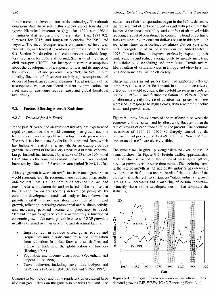
by aviation on the order of 15%, so calculated valueswere scaled up accordingly. By 2015, we assume that theintroduction of advanced air traffic management systemswill reduce this underestimate to approximately 5%. Fullimplementation of these systems by 2050 should reducethe error somewhat further, but given the wide range ofyear 2050 scenario projections, adjustments to calculatedfuel values in 2050 were not considered to be necessary.

Aircraft Emissions: Current Inventories and Future Scenarios

9.1. Introduction

The nature and composition of aircraft emissions has beendescribed in Chapter 1, and their effects on the composition ofthe atmosphere are described in Chapters 2 and 3. Chapter 4uses aircraft emissions data in modeling studies to providechemical perturbations that feed into the ultraviolet (UV)irradiance and radiative forcing calculations presented inChapters 5 and 6, respectively. In this chapter, the aircraftemissions data that were used in calculations described inChapters 4 and 6 are presented and discussed.

Compilation of global inventories of aircraft NOx emissionshas been driven by requirements for global modeling studies ofthe effects of these emissions on stratospheric and troposphericozone (03), Aircraft carbon dioxide (C02) emissions are easilycalculated from total fuel burned. Early studies used one- (I-D)and two-dimensional (2-D) models of the atmosphere (seeSection 2.2.1). Most of these early studies considered effectson the stratosphere (e.g., COMESA, 1975), but some alsoincluded assessments of the (then) current subsonic fleet on theupper troposphere and lower stratosphere (e.g., Hidalgo andCrutzen, 1977; Derwent, 1982). An early height- and latitude­dependent emissions inventory of aircraft NOx was given byBauer (1979), based on earlier work by A.D. Little (1975). Thiswork was used by Derwent (1982) in a 2-D modeling study ofaircraft NOx emissions in the troposphere.

Later estimations of global aircraft emissions of NOx were stillmade by relatively simple methods, using fuel usage and assumedEI(NOx) (e.g., NUBer and Schmitt, 1990; Beck et at., 1992).Concerted efforts were subsequently made by a number of groupsto construct high-quality global 3-D inventories of aircraftemissions. Such work was undertaken for a variety of programsand purposes: United Kingdom input to ICAO Technical WorkingGroups (McInnes and Walker, 1992); the U.S. AtmosphericEffects of Stratospheric Aircraft (AESA) Program (Wuebbles etat., 1993); the German "Schadstoffe in der Luftfahrt" Program(Schmitt and Brunner, 1997); and the ANCATJEC EmissionsDatabase Group (ANCATJEC, 1995), which combined Europeanefforts to produce an aircraft NOx inventory for the AERONOXProgram (Gardner et at., 1997). Subsequently, methodologies forthe production of global 3-D inventories of present-day aircraftNOx emissions (based on 1991-92) have been refined and haveproduced results that have largely superseded earlier work. Theseinventories cover the 1976-92 time period and have been extendedto the 2015 forecast period. These gridded inventories-whichcalculate aviation emissions as distributed around the Earth interms of latitude, longitude, and altitude- have been produced byNASA, DLR, andANCATJEC for national and international workprograms (Baughcum et at., 1996a,b; Schmitt and Brunner, 1997;Gardner, 1998).

This chapter is not the first attempt to synthesize informationon aircraft emissions inventories; earlier assessments weremade by the World Meteorological Organization (WMO)IUnited National Environment Programme (UNEP) (1995)Scientific Assessment of Ozone Depletion, ICAO's Committee

295

on Aviation Environmental Protection (CAEP) Working Group 3(CAEPIWG3, 1995), the NASAAdvanced Subsonic TechnologyProgram (Friedl, 1997), and the European ScientificAssessment of the Atmospheric Effects of Aircraft Emissions(Brasseur et at., 1998).

Any assessment of present and potential future effects ofsubsonic and supersonic air transport emissions relies heavilyon input emissions data. Thus, considerable effort has beenexpended on understanding the accuracy of present-day inventoriesand the construction of forecasts and scenarios. Forecasts arequite distinct from scenarios, as noted in Chapter 1. Forecastsof aviation emissions for a 20-25 year time frame are generallyconsidered possible, whereas such confidence is not the casefor longer time frames. Thus, scenarios generally rely on manymore assumptions and are less specific than forecasts.

In planning this Special Report, it was clear that there were nogridded emission scenarios of NOx emissions from subsonicaircraft for the year 2050 that could be used as input to 3-Dchemical transport models (see Chapters 2 and 4). The IPCCmade a request to ICAO to prepare 3-D NOx scenarios, whichwas carried out under the auspices of ICAO's FESG (CAEP/4­FESG, 1998). The UK DTI also responded to this requirement,producing an independent 3-D NOx scenario for 2050 (Newtonand Falk, 1997). The EDF had also published scenarios ofaircraft emissions of NOx and CO2 extending to 2100(Vedantham and Oppenheimer, 1994, 1998), but these scenarioswere not gridded; thus, although the aviation CO2 scenarioscould be used in radiative forcing calculations (see Chapter 6),the NOx scenarios could not be used to calculate 0 3 perturbationsand subsequent radiative forcing. Other scenario data exist foraircraft emissions, including those from WWF (Barrett, 1994)and MIT (Schafer and Victor, 1997). As with the EDF data,these scenarios were not gridded for NOx emissions, thereforecould not be used in 0 3 perturbation calculations in Chapter 4.Furthermore, the MIT data do not explicitly represent aircraftemissions; instead, they cover high-speed transport modes,including some surface transportation modes.

HSCT scenarios prepared for NASA's AESA Program areconsidered distinct from subsonic scenarios; these HSCTscenarios represent a technology that does not yet exist butmight be developed. Therefore, the HSCT scenarios representa quite different set of assumptions from other long-termscenarios, which only consider continued development of asubsonic fleet. The HSCT scenarios were used in modelingstudies (Chapters 4 and 6) as sensitivity analyses for studyingthe effects of their emissions on stratospheric 0 3 ,

In this chapter, methodologies of inventory and forecastconstruction are compared, and a review and assessment oflong-term scenarios and their implicit assumptions provided.This is the first detailed consideration of long-term scenariosand their implications.

By way of background, Section 9.2 provides an overview offactors that affect aircraft emissions, such as market demand

296

for air travel and developments in the technology. The aircraftemissions data discussed in this chapter are of four distincttypes: Historical inventories (e.g., for 1976 and 1984);inventories that represent the "present day" (i.e., 1991-92);forecasts for 2015; and long-term scenarios for 2050 andbeyond. The methodologies and a comparison of historical,present-day, and forecast inventories are presented in Section9.3. Section 9.4 describes and comments on available long­term scenarios for 2050 and beyond. Scenarios of high-speedcivil transport (HSCT) that incorporate certain assumptionsabout the development of a supersonic fleet and its impact onthe subsonic fleet are presented separately in Section 9.5.Finally, Section 9.6 discusses underlying assumptions anddrivers of long-term subsonic scenarios. The plausibility of theassumptions are also considered in terms of implications forfleet size, infrastructure requirements, and global fossil-fuelavailability.

9.2. Factors Affecting Aircraft Emissions

92.1. Demandfor Air Travel

In the past 50 years, the air transport industry has experiencedrapid expansion as the world economy has grown and thetechnology of air transport has developed to its present state.The result has been a steady decline in costs and fares, whichhas further stimulated traffic growth. As an example of thisgrowth, the output of the industry (measured in terms of tonne­km performed) has increased by a factor of 23 since 1960; totalGDP, which is the broadest available measure of world output,increased by a factor of 3.8 over the same period (ICAO, 1997a).

Although growth in world air traffic has been much greater thanworld economic growth, economic theory and analytical studiesindicate that there is a high correlation between the two, andmost forecasts of aviation demand are based on the premise thatthe demand for air transport is determined primarily byeconomic development. Statistical analyses have shown thatgrowth in GDP now explains about two-thirds of air travelgrowth, reflecting increasing commercial and business activityand increasing personal income and propensity to travel.Demand for air freight service is also primarily a function ofeconomic growth. Air travel growth in excess of GDP growth isusually explained by other economic and structural factors:

• Improvement in service offerings as routes andfrequencies and infrastructure are added, stimulationfrom reductions in airline fares as costs decline, andincreasing trade and the globalization of business(Boeing, 1998)Population and income distribution (Vedantham andOppenheimer, 1998)

• Travel behavior, including travel time budgets andtravel costs (Zahavi, 1981; Schafer and Victor, 1997).

Changes in technology and in the regulatory environment havealso had great effects on the growth in air travel demand. The

Aircraft Emissions: Current Inventories and Future Scenarios

modem era of air transportation began in the 1960s, driven bythe replacement of piston-engined aircraft with jet aircraft thatincreased the speed, reliability, and comfort of air travel whilereducing the cost of operation. The continuing trend of decliningfares (as measured in constant dollars) began in this period. Inreal terms, fares have declined by almost 2% per year since1960. Deregulation of airline services in the United States in1978 allowed airlines to improve services by expanding theirroute systems and reduce average costs by greatly increasingthe efficiency of scheduling and aircraft use. Trends towardliberalization of airline services in Europe and elsewhere willcontinue to increase airline efficiency.

Sharp increases in oil prices have had important (thoughtemporary) effects on traffic demand. In addition to an adverseeffect on the world economy, the lO-fold increase in crude oilprices in 1973-74 and further escalation in 1979-81 (sinceameliorated) greatly increased aviation fuel prices. Air faresincreased in response to higher costs, with a resulting declinein demand growth rates.

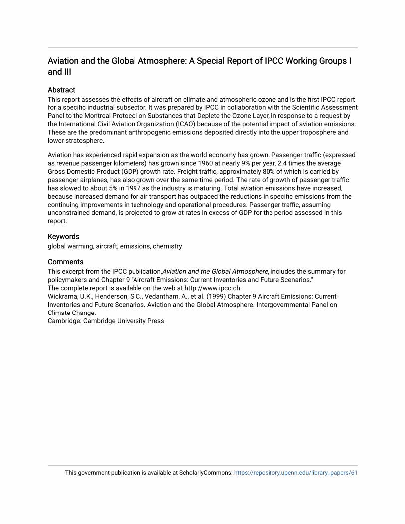
Figure 9-1 provides evidence of the relationship between theeconomy and traffic demand by illustrating fluctuations in therate of growth of each from 1960 to the present. The economicrecessions of 1974-75, 1979-82 (largely caused by theincrease in oil prices), and 1990-91 (the Gulf War) and theirimpact on air traffic are clearly visible.

The growth rate in global passenger demand over the past 35years is shown in Figure 9-2. Freight traffic, approximately80% of which is carried in the bellies of passenger airplanes,has also grown over the same time period. The declining trendin the rate of growth as the size of the industry has increasedby more than 20-fold is a natural result of the total size of theindustry (it is difficult to sustain an "infant industry" growthrate as size increases) and a maturing of certain markets­primarily those in the developed world - that dominate thestatistics.

20

/\/\I \

15I "I \---~ I \-'-' I Tonne-km \ I~ 10 \ I \ I~

= \ \ II:Il.: \ ,U ~-; 5===~ Real GDP

0

-51960 1965 1970 1975 1980 1985 1990 1995

Year

Figure 9-1: Relationship between economic growth and trafficdemand growth (IMF, WEFA, ICAO Reporting FormA-I).

Aircraft Emissions: Current Inventories and Future Scenarios 297

16

Section 9.3). A discussion of the technology required to reduceNOx emissions while continuing to improve engine efficiencyappears in Chapter 7.

Figure 9-2: Growth rate of passengers carried (ICAOReporting Form A-I). Note the assumption of 5-year movingaverage of annual growth rates, excluding operations in theCommonwealth of Independent States (CIS).

1995

... .+"+.:

..".. ..+ +••

,......'.'.

, ..... .... .~ .......

•...'..

... / Passengers Carried

\~

1965 1970 1975 1980 1985 1990Year

o1960

Changes in demand in regional markets are given in Table 9-1for the period 1970-95. Over this period, global traffic measuredin revenue passenger kilometers (RPK) increased by a factor of 4.6(Boeing, 1996). Table 9-1 is ordered by 1995 regional RPK value.

The growth rate of fuel consumed by aviation therefore hasbeen lower than the growth in demand. Improvement in enginefuel efficiency has come mainly from the increasing use ofmodem high-bypass engine technology that relies on increasingengine pressure ratios and higher temperature combustors as ameans to increase engine efficiency. These trends have resultedin drastic decreases in emissions of carbon monoxide (CO) andunburned hydrocarbons (HC), though they tend to increaseemissions of oxides of nitrogen (NOx)' As a result, total NOx

emissions from aircraft are growing faster than fuel consumption(see Figure 9-4, from NASA emissions inventories discussed in

The trend in fuel efficiency of jet aircraft over time has been oneof almost continuous improvement; fuel burned per seat intoday's new aircraft is 70% less than that of early jets. About40% of the improvement has come from engine efficiencyimprovements and 30% from airframe efficiency improvements(Figure 9-3, after Figure III-A-l in Albritton et. ai, 1997).

922. Developments in Technology

Table 9-1: Regional share of total demand.

1970-95 1970 1995 1970-951970 1995 Growth Market Market Change in

Regional Traffic Flow RPKx 109 RPK x 109 Factor Share Share Share

Intra North America 190.897 697.880 3.7 34.6% 27.5% -7.1%Intra Europe 61.275 317.099 5.2 11.1% 12.5% 1.4%North America - Europe 72.143 277.909 3.9 13.1% 11.0% -2.1 %China Domestic/Intra Asia/Intra Oceania 10.234 207.405 20.3 1.9% 8.2% 6.3%North America - Asia/Oceania 14.760 188.799 12.8 2.7% 7.4% 4.8%Europe - Asia 6.732 134.343 20.0 1.2% 5.3% 4.1%Asia - India/Africa/Middle East 13.959 115.204 8.3 2.5% 4.5% 2.0%North America - Latin America 16.087 75.538 4.7 2.9% 3.0% 0.1%Europe - Latin America 7.124 73.090 10.3 1.3% 2.9% 1.6%Domestic Former Soviet Union 75.496 67.603 0.9 13.7% 2.7% -11.0%Japan Domestic 8.181 61.607 7.5 1.5% 2.4% 0.9%Europe - Africa 18.478 61.045 3.3 3.4% 2.4% -0.9%Intra/Domestic Latin America 13.432 55.331 4.1 2.4% 2.2% -0.3%Europe - Middle East 9.838 41.224 4.2 1.8% 1.6% -0.2%Intra/Domestic Middle East - Africa 5.065 39.213 7.7 0.9% 1.5% 0.6%International Former Soviet Union 3.677 29.508 8.0 0.7% 1.2% 0.5%Indian Subcontinent - AsialMiddle East/Oceania 3.249 29.500 9.1 0.6% 1.2% 0.6%Europe - Indian Subcontinent 2.333 19.858 8.5 0.4% 0.8% 0.4%Intra/Domestic Africa 5.826 16.808 2.9 1.1% 0.7% -0.4%Intra Indian Subcontinent 3.215 13.218 4.1 0.6% 0.5% -0.1%North America - Africa/Middle East 1.149 10.777 9.4 0.2% 0.4% 0.2%U.S. Military Airlift 8.112 3.605 0.4 1.5% 0.1% -1.3%

Total 551.262 2536.561 4.6 100.0% 100.0% 0.0%

20001990

Engine FuelConsumption

B747-100Bi

IIIIB747SP

Aircraft Emissions: Current Inventories and Future Scenarios

DClO-30

1970 1980Year of Model Introduction

l1liB747-100 ~ B747-200

DC8-63l1li

Comet 4

1960

B707-120B •

1707!;O

B707-120 oeD DC8-30

DC8~61. SVClO. B747-200 ·UDClO-30....., B7:;;-20OB(IDB747-300 B747-400 IB707-320B. A3lO-3000 001 A330-3~'

+-------+-------"""i-------.-+----....:A300-600R . r::r 0 IIA340-300 B777-2OO IAircraft FuelBurn per Seat

.B747-2OOB 0A3~-600B -*-18B747-300 I ,.

A3lO-3001111 l1li. A340-300 l1lil1li I+---------+--------I---------+------B747-400-A330-300 l1li !

B777-200 I!

B707B~%~_3!O.LDC8-30 SVCI0B707-120BrOO ODC8-63

+- DC8-61 B707-320B

I

298

100

90

80

~

.". 70....IlJe0u'-' 60IlJ

'"~=:l....0 50~

40

30

20

1950

Figure 9-3: Trend in transport aircraft fuel efficiency.

9.3. Historical, Present-Day, and 2015Forecast Emissions Inventories

Studies on the effects of CO2 emissions from aircraft on radiativeforcing require only a knowledge of total emissions. However,to examine the potential effects of other emissions from aviation(e.g., those considered in Chapter 4), estimates of the amountand the distribution of emissions are required. Such 3-Dinventories for present and projected future aviation operationshave been produced under the aegis of NASA's AtmosphericEffects of Aviation Project (AEAP), the European CivilAviation Conference's ANCAT and EC Emissions InventoryDatabase Group (EIDG), and DLR.

These inventories consist of calculated aircraft emISSIOnsdistributed over the world's airspace by latitude, longitude, andaltitude. Historical inventories of aviation emissions have beenproduced for 1976 and 1984 by NASA. Present-day and 2015forecast inventories (where present-day is taken to be the mostrecent available-1991-92) have been produced by NASA,ANCAT, and DLR. DLR has also produced emissions inventoriesof scheduled international aviation only for each year from1982 through 1992, and for total scheduled aviation for 1986and 1989. DLR has also constructed a four-dimensional (4-D)inventory with diurnal cycles for scheduled aviation in March 1992.

All of the aforementioned 3-D emissions inventories have acommon approach of combining a database of global air traffic

(fleet mix, city-pairs served, and flight frequencies) with a setof assumptions about flight operations (flight profiles and routing)and a method to calculate altitude-dependent emissions ofaircraft/engine combinations in the fleet. Figure 9-5 shows howthese processes are combined.

All of the historical, present-day, and 2015 forecast inventoriesconsidered in this section assume idealized flight routingsand profiles, with no winds or system delays. Thus, minimum

7~

~ 6'-'IlJ.... 5~

~

-= 4....~

83~

IlJOIl~ 2"'"IlJ

~ 1

0Calculated Calculated Forecast1976-1984 1984-1992 1992-2015

Time Period

Figure 9-4: Comparison of growth rates for civil traffic, fuelconsumption, and NOx emissions.

Aircraft Emissions: Current Inventories and Future Scenarios 299

fuel burn and emissions possible for each flight operationare implicit, given the onboard load assumed. Simplifyingassumptions for military operations vary according to aircrafttype.

93.1. NASA,ANCAT/EC2, and DLRHistorical and Present-Day Emissions Inventories

The NASA,ANCAT, and DLR 3-D inventories adopt a similaroverall approach but differ in some of the components and dataused. This section describes the common approaches andexplains the differences. More detailed information appears inthe source material for these inventories (Baughcum et al.,1996a,b; Schmitt and Brunner, 1997; Gardner, 1998).

Different approaches were taken for constructing underlyingtraffic movements databases. The NASA inventories usescheduled jet and turboprop aviation operations for the years1976,1984, and 1992 (Baughcum et al., 1996a,b). Movementsfor charter carriers, military operations, general aviation, andthe domestic fleets of the former Soviet Union (FSU) and thePeople's Republic of China were estimated separately (Landauet al., 1994; Metwally, 1995; Mortlock and VanAlstyne, 1998).Military aircraft contributions to emissions were calculated byestimating the flight activity of each type of military aircraft bycountry. The 1976 and 1984 NASA inventories were based onoperations for 1 month in each quarter of the year, whereas the1992 inventory compiled movements on a monthly basis toreflect the seasonality of aviation operations.

All of the inventories use a "bottom-up" approach in which anaircraft movement database was compiled, aircraft/enginecombinations in operation were identified (to differing levelsof detail), and calculations of fuel burned and emissions alonggreat-circle paths between cities were made. Flight operationdata were calculated as the number of departures for each citypair by aircraft and engine type-which, combined withperformance and emissions data, gave fuel burned and emissionsby altitude along each route. This approach resulted in data onfuel burned and emissions of NOx (as NOz) on a 3-D grid foreach flight. In addition, the NASA inventories provide 3-Ddistributions of CO and total HC. NASA and ANCAT inventorieswere calculated on a 10 longitude x 10 latitude x l-km altituderesolution, whereas the DLR inventory used a 2.80 longitude x2.80 latitude horizontal resolution.

The ANCAT approach used a combination of air traffic control(ATC) data and scheduled movements, favoring ATC datawhere available (Gardner, 1998). Where ATC data wereunavailable, scheduled data were taken from the ABC TravelGuide (ABC), the Official Airline Guide (OAG), the Aeroflottime table, and a German study of Chinese domestic aircraftmovements. Only jet aircraft were represented in theANCAT/EC2 inventory. The most significant omission of ATCdata was the United States, for which data were unavailable forsecurity reasons. Thus, only time table data were used for theUnited States; so nonscheduled U.S. domestic charters andother flights were not recorded. To compensate for this problem,fuel usage data were factored up by 10% (Gardner, 1998). ATCdata accounted for half of the non-U.S. aircraft movements inthe database. Military movements were estimated by allocatingfuel and emissions to countries' boundaries from an analysis of

the world's military fleetcomposition.

Figure 9-5: Aircraft emissions inventory calculation schematic.

GLOBAL AIRCRAFT EMISSIONS INVENTORY

I Airplane Performance DatabaseThe DLR inventory for1991/92 (Schmitt and Brunner,1997) used the ANCAT/EC2civil movements database.Emissions inventories for1986, 1989, and 1992 werebased on scheduled air trafficonly; a 4-D inventory withdiurnal cycles for March1992 was based onABC data.ICAO data (ICAO, 1997b)were used for emissionsinventories for international(only) scheduled air traffic inthe years 1982 to 1992.

Calculation of fuel burnedand emissions for aircraft differsbetween the three inventories.NASA used detailedmanufacturers' proprietaryperformance information on eachaircraft-engine combinationand the flight profile shown

/Emissions

Models

IEngine Emissions Database

/Performance

Models

General Aviation

Charter Service

Flight Operations

Scheduled Service

Military

300 Aircraft Emissions: Current Inventories and Future Scenarios

in Figure 9-6. Emissions were calculated from the informationin the ICAO Engine Exhaust Emissions Data Bank (lCAO, 1995),through the use of Boeing "Method 2" procedures (Baughcumet at., 1996b, Appendix D), which allow extrapolation of sea­level data in the ICAO data bank to the operating altitudes andtemperatures encountered throughout the aircraft flight profile.

The ANCATlEC2 inventory used commercial software forflight and fuel profiling, along with Project Interactive Analysisand Optimization (PIANO), a parametric aircraft design model.The global civil fleet was modeled with a selection of 20representative aircraft types. These representative aircraftwere assumed to be fitted with generic engines typical of thetechnology and thrust requirements of each type. PIANOgenerated fuel profiles covering the entire flight cycle, includingsteps in cruise for each aircraft. Fuel use during ground operationswas estimated from ICAO certification timings (ICAO, 1993).

The DLR inventory used airline data and an in-house flight andfuel profile model (Deidewig et at., 1996). The DLR approachalso used different aircraft/engine combinations from thoseutilized by ANCAT. The aircraft mission was simulated by usinga simplified flight modeling code as point-to-point missions withno step cruise. Although the climb was calculated in iterativesteps, the cruise segment was treated as one section, applyingthe Breguet formula to calculate the cruise fuel. Descent wasassumed to be a gliding path with minimum engine load; noseparate approach procedure was used. A thermodynamicmodel for design and off-design operation of a two-shaft fanengine was applied. Constant efficiencies and constant relative

pressure losses for main engine components were assumed forsimplicity.

The ANCAT/EC2 and DLR inventories calculated NO,emissions from the fuel using the DLR fuel flow method. Thismethod has been tested and correlated with information fromairlines, flight measurements, and altitude chamber measurements(Deidewig et at., 1996; Schulte et at., 1997).

9.3.2. NASA,ANCATIEC2, and DLR2015 Emissions Forecasts

The first NASA subsonic aircraft emissions inventory for 2015was created as part of an assessment of the effects of a futureHSCT (Baughcum et at., 1994); it has now been superseded bya new study (Baughcum et at., 1998; Mortlock and VanAlstyne, 1998) that includes new emissions technologyassumptions and more detailed fleet mix and route systemcalculations. The NASA 2015 forecast inventory was calculatedusing methods similar to those used for NASA's historical andpresent-day inventories. Separate forecasts were created forscheduled operations (flights shown in the OAG database),charter operations, cargo operations, domestic operations in theFSU and China, military operations, and general aviation.

The forecast for scheduled traffic was based on the 1996Boeing Current Market Outlook (Boeing, 1996), which projectsseparate traffic growth rates by region. Growth in worldwidedemand for air travel was expected to average about 5% per

Typical Mission Rules With 200-nmi Alternate

1,500 ft

10,000 ft

Reserves.

'Speed restrictions as applied to mission

I~ 200nmi~ I......----- Reserve fuel ...

MissionI

~

00

C/o q,"0 0 .:IolI': ,....,~ C/o I':0 "0 ~

<n I': "0

N ~ III <n

B III C/o N0 .....<n

p., 0 'iiJ ----

*N

C/o

~C/o

.0 ~ III'iiJ ,2 ;>.... 0 0 ....III~

<n 0 IIIV U N C/o<n

~(j 0 B B(j 0CIl q,

*B " a

~ 0 I': 0.... " ..os ~0 BIII I':

0 V III I': V~

(j

I': "l .0 (j C/o 's c8<n .2III III'8 r<) Cl Cl <n

.......<::

0\ B 0 10,000 ft .8 0/)

S i:l:: 'R rB0 0

~t9III'R ~ <n

~ ~

I~I~ Still air range ... ,

...1 JFlight fuel and time

.... Block fuel and time

Figure 9-6: Scheduled aircraft mission profile.

Aircraft Emissions: Current Inventories and Future Scenarios 301

noise. The CAEP/2 designation refers to emissions certificationstandards adopted at the second meeting of the CAEP inDecember 1991.) Much more of the fleet consists of low-NOx

aircraft-engine combinations in 2015, with ~70% of fuelburned in engines with NOx emission levels between 20 and40% below the CAEPI2 certification limit.

DTI has developed a traffic and fleet forecast model for civilaviation, which was adapted under the direction of ANCAT andEIDG to produce an estimate of fuel burned and NOx emittedby civil aviation for the forecast year of 2015 (Gardner, 1998).Fuel and NOx growth factors-base to forecast-were calculatedand applied to the ANCAT/EC2 city-pair gridded 1992 baseyear inventory to produce a gridded 2015 forecast.

20152005

~ History Forecast--..

1975

~ 8000 ...----------.,----------,[IJ

.§ 7000=6e 000

~ 5000

~ 4000, 3000

't:l§ 2000

5 1000 b::::::::::::CdNdWCJdJd4dJIi'ldgHi'f':':: t' ...Q OL.-~-...........-_-_---4-_-__........---l

1985 1995Year

Figure 9-7: Passenger traffic demand growth to 2015.

year to the year 2015, with international travel growing at aslightly faster rate than domestic travel (Figure 9-7). By 2015,demand for air travel is projected to be 2.5 times greater thanin 1996.

The total projected demand for scheduled air travel in the year2015 was assigned to actual aircraft on a projected city-pairschedule derived from the schedules for 1995 published in theOAG. Individual city-pair service schedules for 1995 withineach of the traffic flow regions were grown to 2015 by usingthe consolidated regional growth rate applicable for thatregion. Aircraft types were assigned to routes by using a marketshare forecast model. The turboprop market (for which therewas no detailed forecast) was projected for 2015 by assumingthat city pairs not served by the smallest turbojet category(50-90 seats) after demand growth to 2015 will continue to beserved by small, medium, or large turboprops.

The result of the fleet assignment task was a detailed city-pairflight schedule by aircraft type required to satisfy forecastscheduled passenger demand in 2015. This schedule was usedto calculate the 3-D emissions inventory for scheduled passengerservice. Simplifying assumptions were the same as those usedin calculating the historical and present-day inventories.

DTI's top-down regional traffic demand forecasting model hasa horizon of 25 years. Traffic coverage in the model includesall scheduled civil operations but excludes the former SovietUnion, Eastern Europe, freight, military, non-European chartertraffic, business jets, and general aviation. Factors were developedto account for these traffic sectors in the forecast. The trafficforecast assumes a relationship between traffic [available seat­kilometers (ASK)] and GDP growth, and is assessed on aregional and flow basis (i.e., traffic flow between specificregions). The relationship is modified by assumptions on airlineyie1ds-a surrogate for fares price-and by a market maturityterm that modifies demand as a function of time. Future fleetsare estimated from traffic forecasts in terms of size andcomposition.

The concept of "traffic efficiency" was used to estimate fuelconsumption from traffic values. Traffic efficiency is definedas the amount of traffic or capacity (ASK) per unit of fuelconsumed. Aircraft manufacturers' traffic efficiency data forcurrent aircraft types and projections for future aircraft typeswere used to develop efficiency trends for the eight categoriesof generic aircraft adopted for forecasting purposes, over arange of flight sector lengths. This approach permitted estimationof fuel consumption on the basis of regional and global trafficforecasts.

0% 10% >20%to 10% t020%

LTO NOx Relative to CAEP/2 Limit

Figure 9-8: Percentage of total scheduled fleet fuel burnedby aircraft in specific LTO NOx emissions categories for May1992 (Baughcum et at., 1996b) and the year 2015 projection(Baughcum et at., 1998).

~ 40~ 35'-'

= 30•:=~ 25~

~ 20.... IS~~

rz 10-; 5....~ 0

-50% -40% -30% -20% -10%to -40% to-30% to -20% to -10% toO%

Projections of engine and aircraft technology levels for the2015 scheduled fleet with regard to fuel efficiency and NOx

emissions were made by assuming a continuation of presenttrends. In general, engines in the 2015 scheduled fleet representthe state-of-the-art in engine technology available either inproduction or in the final stages of development at the time theassignments were made (1997). These engines include low­emissions derivatives of previously existing engines. It isunlikely that any radical changes in airframe or enginedesign- even if such designs were acceptable - would havemuch of an effect on the 2015 fleet, given the time required tobring new designs into service. The combined effects of 2015fleet mix and technology projections on the NOx technologylevel of the projected 2015 fleet appear in Figure 9-8, whichshows the percentage of total fleet fuel burned by aircraft havinglanding/take-off cycle (LTO) emissions at a given level relativeto the CAEP/2 NOx limit. (CAEP is chartered to proposeworldwide certification standards for aircraft emissions and

302 Aircraft Emissions: Current Inventories and Future Scenarios

Table 9-2: Future trends in fuel efficiency improvement.Average efficiency figures were also calculated for the eightgeneric aircraft types in the 1992 base year fleet; a fleet averagevalue of about 24.0 seat-km per liter was found. This figurecompares well with those in Greene (1992) and Balashov andSmith (1992) for the years 1989 and 1990, respectively, whichgave traffic efficiencies of 20.5 seat-km per liter.

Time Period

1993-20002000-20102010-2015 (extrapolation)

Fuel Efficiency Improvement

1.3% yr-!1.3% yr-!1.0% yr-1

Greene (1992) and Balashov and Smith (1992) forecast anannual improvement in commercial air fleet fuel efficiency(see Table 9-2). These efficiencies include improvements arisingfrom the introduction of new aircraft into the fleet and changesto operating conditions and passenger management. For theDTI work, the Greene (1992) forecasts were used to 2010.Annual improvements in fuel efficiency was assumed todecrease to 1% per year beyond 2010.

Using this efficiency trend, traffic efficiencies were calculatedfor the future aircraft fleet. The base year fleet average wasestimated to increase to 31.8 seat-km per liter by 2015.

The same trends in fuel efficiency were applied to all size andtechnology classes. This approach represents a simplificationbecause improvement figures are really a fleet average andwould be influenced strongly by the rate of introduction of newaircraft. Given the much smaller contribution of older aircraftto global traffic performance, however, this factor will be onlya second-order effect.

The emission performance of the forecast fleet was determinedin part by the assumed response of the engine manufacturingindustry to an assumed regulatory scenario. An emissionscertification stringency regime was proposed for the forecastperiod, and compliance with the tighter limits was achieved bymodifying the emissions performance of engines as theybecame noncompliant. This calculation was assessed from abase year engine fleet, comprising engines typical of andrepresenting those found in the fleet (and compatible withthe aircraft generic types described above). Performanceimprovements were applied only to new fleet entrants and wereappropriate for staged and ultra-low NOx control technology insome cases.

This process results in an estimate of fuel burn and NOx

emissions for the base year and forecast fleet using the samemethodology; 1992-2015 fuel and NOx growth factors arethereby calculated. The growth factors were applied to theANCAT/EC2 base year gridded fuel and NOx estimates toprovide a 2015 gridded forecast.

93.3. Other Emissions Inventories

Studies of atmospheric effects of aviation were conductedusing the global inventory of McInnes and Walker (1992) andemissions data sets produced by the Dutch Institute of PublicHealth and Environmental Protection for 1990,2003, and 2015(Olivier, 1995) based on the McInnes and Walker (1992) data.Other emissions estimates are predominantly made on anational level (e.g., in Austria and Sweden).

The Dutch Aviation Emissions and Evaluation of ReductionOptions (AERO) Project was initiated in 1994 by the Dutch CivilAviation Department to estimate economic and environmentalimpacts of possible measures to reduce aviation emissions (seeChapter 10). Within this project, the flights and emissions model(FLEM) was developed for the calculation of worldwide fueluse and emissions per grid cell (ten Have and de Witte, 1997).The base year traffic movements database is a combination ofdata from ANCATIEC2, International Air Transport Association,the ABC schedule, ICAO, and the U.S. Department ofTransportation (DOT). Global volumes for aircraft kilometer,fuel consumption, and emissions (C02 , NOx) resulting fromcomputations of the AERO modeling system for civil aviationfor base year 1992 and forecast for 2015 (called FPC-2015scenario) are listed in Table 9-3. Further details appear inPulIes (1998).

9.3.4. Comparisons ofPresent-Day and 2015Forecast Emissions Inventories(NASA,ANCAT/EC2, and DLR)

Table 9-4 lists the totals for calculated fuel burned and emissionsfrom the NASA,ANCAT, and DLR inventories for 1976, 1984,1992, and 2015. Because these inventories consisted of 3-D

Table 9-3: Results from AERO modeling analysis.*

*AERO results for base and datum (FPC-20IS scenario).

1992 2015The methods used to project civil aviation traffic demand forthe DLR 2015 inventory were based on regional growth factorscalculated by DTI. Thus, the DLR 2015 forecast differs fromthe ANCATlEC2 forecast only in that the base year inventoryis slightly different because of the different fuel and profilingmethodology and the aircraft generic types. Thus, in thecomparison of results, ANCAT and DLR 2015 forecasts are notassumed to be different because the DLR forecast is essentiallyan application of the DTI/ANCAT forecast.

Aircraft kilometers (km yr-!)Fuel consumption (Tg yr-!)CO2 emissions (Tg yr-!)NOx emissions (Tg yr-!)

20.7 X 109

1444531.84

49.6 X 109

2788773.86

AnnualChange

3.9%2.9%2.9%3.3%

Aircraft Emissions: Current Inventories and Future Scenarios 303

Table 9-4: Calculated fuel and emissionsjrom NASA, ANCAT, and DLR inventories.

NASA NASA NASA ANCAT DLR NASA ANCAT DLR1976 1984 1992 1992 1992 2015 2015 2015

Calculated Fuel Burned (Tg)Scheduled 45.83 64.17 94.84 252.73Charter 8.47 9.34 6.57 13.50FSU/China 6.05 7.43 8.77 15.79General Aviation 4.04 5.62 3.68 6.03

Civil Subtotal 64.38 86.56 113.85 114.20 112.24 288.05 272.32 270.50Military 35.66 29.76 25.55 17.08 17.10 20.59 14.54 14.50

Global Total 100.04 116.31 139.41 131.3 129.34 308.64 287.86 285.00

Calculated CO2 Emissions (Tg C)Scheduled 39.41 55.18 81.56 217.35Charter 7.28 8.03 5.65 11.61FSUlChina 5.20 6.39 7.54 13.58General Aviation 3.47 4.83 3.16 5.18

Civil Subtotal 55.36 74.44 97.91 98.22 96.52 247.72 234.21 232.63Military 30.67 25.59 21.98 14.68 14.71 17.71 12.50 12.47

Global Total 86.03 lOOm 119.89 112.92 111.23 265.43 246.71 245.10

Calculated NOx Emission (Tg as N02)

Scheduled 0.50 0.79 1.23 3.57Charter 0.09 0.11 0.09 0.19FSU/China 0.04 0.06 0.06 0.12General Aviation 0.06 om 0.05 0.07

Civil Subtotal 0.70 1.02 1.44 1.60 1.60 3.95 3.37 3.41Military 0.28 0.25 0.23 0.20 0.20 0.18 0.16 0.16

Global Total 0.98 1.28 1.67 1.81 1.80 4.12 3.53 3.57

Calculated Fleet Average NOx Emission Index [g NOx (as N02) kg-1 fuel burned]Scheduled 10.9 12.3 13.0 14.1Charter 10.8 11.3 13.3 13.8FSU/China 7.4 7.4 7.4 7.4General Aviation 14.5 12.6 14.4 11.3

Civil Subtotal 10.8 11.8 12.6 14.0 14.2 13.7 12.4 12.6Military 8.0 8.5 8.9 11.9 11.8 8.7 10.7 10.8

Global Total 9.8 11.0 12.0 13.8 13.9 13.4 12.3 12.5

data sets, the differences in spatial distributions as well astotals are compared. The NASA inventories also includedemissions of CO and HC, which are summarized in Table 9-5.

The NASA inventories include piston-powered aircraft in thegeneral aviation fleet. This category of aircraft is excludedfrom the ANCAT and DLR inventories, but the contribution tototal fuel burned from these aircraft is small (2.6% of fuelburned in 1992). Piston-powered aircraft are large contributorsto CO and HC emissions relative to the amount of fuel theybum (39% of CO and 13% of HC emissions in 1992). Thislarge relative contribution is reflected in the emissions indicesof these two pollutants in the general aviation category.

A comparison of calculated global total values for fuel burned andNOx emissions from the NASA, ANCAT, and DLR inventories

for 1992 and 2015 is shown in Figure 9-9. All three inventoriesfor 1992 have approximately the same calculated values for totalfuel burned in the civil air fleet; the difference in total fuel (7%maximum) arises almost entirely from different calculatedcontributions for military aviation operations, for which theANCAT inventory calculates 33% lower fuel burned. Becausemilitary fuel is estimated to be between 13 and 18% of total fuelin 1992, the effect of this large difference in estimates betweenmilitary sectors on the total is small. Use of the NASA inventoriesas a base is arbitrary and does not imply that differences from theNASA results are errors. Exclusion of turboprop operations fromthe ANCAT inventory results in about a 2% underestimate (ifdata from the NASA inventory are used).

Calculated values for total NOx emissions from the threeinventories for 1992 are within 9% of each other. The ANCAT

304

Table 9-5: Emissions ofco and HC from NASA inventories.

Aircraft Emissions: Current Inventories and Future Scenarios

Calculated Fleet Average HC Emissions Index (g HC kg-] fuel burned)Scheduled 5.8 3.2Charter 0.9 0.9FSu/China 3.2 3.2General Aviation 8.2 8.5

Civil Subtotal 5.1 3.3Military 2.5 2.3

Global Total 4.2 3.0

Calculated Fleet Average CO Emissions Index (g CO kg-] fuel burned)Scheduled 8.9 6.3Charter 4.0 4.0FSu/China 16.6 16.6General Aviation 180.1 133.0

Civil Subtotal 19.7 15.2Military 12.0 11.9

Global Total 17.0 14.4

Calculated CO Emissions (Tg)ScheduledCharterFSU/ChinaGeneral Aviation

Civil SubtotalMilitary

Global Total

Calculated HC Emissions (Tg)ScheduledCharterFSu/ChinaGeneral Aviation

Civil SubtotalMilitary

Global Total

NASA1976

0.41om0.100.731.270.431.70

0.27om0.02om0.330.090.42

NASA1984

0.410.040.120.751.320.351.67

0.20om0.Q20.050.280.070.35

NASA NASA1992 2015

0.50 1.120.02 0.050.15 0.260.62 0.601.29 2.040.29 0.231.57 2.27

5.3 4.53.7 3.9

16.6 16.6167.6 99.4

11.3 7.111.2 11.311.3 7.4

0.20 0.170.00 omom 0.050.04 0.050.26 0.280.06 0.050.32 0.33

2.1 0.70.5 0.63.2 3.29.9 8.62.3 1.02.4 2.52.3 1.1

and DLR values are higher than those from NASA-a result ofa combination of differing fleet mixes, a different method ofcalculating NOx emissions, and the offsetting effects of civiland military calculations. This variation is also reflected in thecalculated EI(NOx) for the fleet components: The ANCAT andDLR inventories have a total fleet emission index that is 15%higher than that of the NASA inventory.

Differences between inventory totals widen for the 2015 case,although total fuel burned is still within 8%. Total NOx

emissions in the NASA 2015 forecast are almost 15% greaterthan those in the ANCAT forecast, a result of differentassumptions about the direction of NOx reduction technology(the NASA assumptions result in an increase in NOx emissionsindex in the civil sector, whereas the ANCAT forecasts assumea reduction).

Other differences between the NASA, ANCAT, and DLRinventories relate to the distribution of calculated fuel burnedand emissions, geographically (latitude and longitude) andwith altitude. Although all three inventories place more than90% of global fuel burned and emissions in the NorthernHemisphere, there are differences between inventories in thedetails of the distribution. Figure 9-10 shows the distribution offuel burned as calculated in 1 month (May) of the 1992 NASAinventory. The most heavily trafficked areas are clearly visible(United States, Europe, North Atlantic, North Asia).

For geographical comparison purposes, data in the files of theNASA and ANCAT 1992 inventories were divided into 36 regions,defined by 60° spans of longitude and 20° spans of latitude.Figure 9-11 shows the differences between the ANCAT andNASA 1992 inventories with regard to geographical distribution.

Aircraft Emissions: Current Inventories and Future Scenarios 305

The major differences between the NASA and ANCAT inventories(on a geographical basis) lie in the estimate of fuel burned andNOx emissions in the regions covering North America andEurope. The ANCAT inventory places 32% of total fuel burnedand 30% of total NOx over North America, whereas the NASAinventory places 27% of fuel burned and 27% of NOx over thatregion. ANCAT places 16% of the fuel and 15% of the NOx overEurope, whereas the NASA inventory places 21 % of the fuel and19% of total NOx over that region. Part of this difference may beexplained by the 10% scaling of U.S. traffic assumed by ANCATas a method of approximating the U.S. charter market.

in Figure 9-12 and for military aviation in Figure 9-13. The civilaviation distributions are similar, with the NASA inventory showingmore fuel burned at higher altitudes. The military distributions arequite different, with fuel burned in the NASA inventory concentratedat the higher altitudes and fuel burned in the ANCAT inventory atlower altitudes. This difference may be because of a higherproportion of transport operations in the NASA inventory. Thealtitudinal distribution of NOx emissions follows closely that offuel burned. The three inventories show that more than 60% of thefuel burned and NOx emissions occur above 8 km, whereas amajor fraction of CO and HC are emitted near the ground.

NASA and ANCAT fuel and NOx emissions projections for2015 are similar to the respective 1992 inventories in that nonew city pairs were used in the 2015 traffic projections. Growthrates from 1992 to 2015 vary with region, so the geographicaldistribution of emissions changes over time.

The altitudinal distributions of fuel burned in the present-dayNASA,ANCAT, and DLR inventories are shown for civil aviation

Although the three inventories show comparably low variationsfor total global monthly figures over the year, the seasonaldependency can be quite large for some regions (Figure 9-14).Operations in the North Atlantic and North Pacific show a clearyearly cycle, with a maximum in the northern summer and aminimum during winter. In contrast, Southern Hemisphereoperations show little seasonal variation overall, with smallpeaks in February and November.

Comparison of Inventories (1992 and 2015) - Fuel Burned

NASA 2015(Base)

• Civil

• Military

• Total

5.--------:-:-=-:-=-:-:::-:::-=-----:::-=-=-~:::_=___.-------:_:_:_:::_:_:~:_:_:,__-:::_:_=___:_:_:~__,

0+-------+- _-5 NASA 1992

-10 (Base)

-15-20-25-30-35 .L:::::=======---__~=_ ~~_-L __.J

Comparison of Inventories (1992 and 2015) - NOx Emissions

• Civil

• Military

• Total

NASA 1992(Base)

NASA 2015(Base)

Comparison of Inventories (1992 and 2015) - NOx Emissions Index

NASA 2015(Base)

DLR 1992

35,-;=========;----;;;:::------:::::---,-------:-::::-:-==-:::-.-:------=:-::-=-:-:--,30 Civil ANCAT 2015 DLR 2015

25 • Military

20 • Total15 J '-----------"

105O+------+--

NASA 1992 ANCAT 1992-5 (Base)-10.1...-------------------------

Figure 9-9: Comparison of inventories.

306 Aircraft Emissions: Current Inventories and Future Scenarios

300 N

~

"Cl.a 0......."=..;I

300 S

1800 W 1500 W 1200 W 900 W 600 W 300 W 0 300 E

Longitude

OD ID 2D 3D 4DloglO Fuel (kg day·l)

Figure 9-10: Geographical distribution of fuel burned by civil aviation (May 1992).

5.0 6.0 7.0

DLR has also examined longer trends in fuel burned and emissionsfor air traffic (Schmitt and Brunner, 1997). 3-D gridded inventoriesof fuel burned and emissions were calculated for 1982 through1992 using ICAO statistics on annual values for internationalscheduled air traffic and ABC time table data of all scheduled airtraffic for the same week of September in 1986, 1989, and 1992.Emissions inventories were produced for each of these data setsusing the same methods as in the 1992 DLR inventory describedabove. These inventories concentrate on scheduled servicesbecause reasonably accurate calculations are possible for thissegment of aviation. Because these data do not include non­scheduled flights, military traffic, general aviation, or former SovietUnion/China traffic, they are of limited use in global modelingstudies. However, they do provide a consistent set of data to trackthe growth of the international and domestic scheduled sector.Table 9-6 gives the totals for the yearly inventories.

93.5. Error Analysis and Assessment of Inventories

Simplifying assumptions used in creating all of the 3-Demissions inventories have introduced systematic errors in the

calculations. An analysis of the effects of the simplifyingassumptions on fuel burned used in the 1992 NASA inventoryhas been performed by Baughcum et at. (1996b). All of theassumptions have the effect of biasing the calculation towardan underestimate of fuel burned and emissions produced, asdetailed in Table 9-7. The effects of the assumptions on theANCAT and DLR inventories may be expected to be similar,because most of the simplifying assumptions used in thoseinventory calculations were similar to those in the NASAinventory.

The assumption of great-circle flight paths results in anunderestimate of distance flown, although the practice ofrouting to take advantage of winds may result in lower fuelconsumption than a great-circle path for a given flight. A studyof international and domestic flights from German airportsshowed an average increase in flight distance of 10% for medium­and long-haul flights above 700 km, with larger deviationsfrom great-circle routes for shorter flights (Schmitt and Brunner,1997). Ground delays and in-flight holding at relatively lowaltitudes caused by congestion in the air traffic control systemalso adds to fuel consumption. Aircraft in service are subject to

Aircraft Emissions: Current Inventories and Future Scenarios

factors that may increase fuel consumption by up to 3% (e.g.,engine deterioration, added weight from added systems, andincreased surface roughness).

307

Factors that cause underestimates of fuel burned do notnecessarily operate at the same time, so they are not additive.Sutkus et al. (1999) compared fuel burned for certain carriers

Latitude

z°o0\

8~

z°or")

8o

Z°~8r:/j

°or")

120 to1800 W

60 to1200 W

15,000,000

10,000,000N

5,000,0000'10'1~

<0 00

<~Z'7-5,000,000 I~

N"ClO'IQJIO'I~

-10,000,000 ~ '-'

~-15,000,000 U

Z<

-20,000,000

-25,000,000

Longitude

Figure 9-11: Differences in geographical distribution of fuel burned.

Ic DLR Civil FuelIl'l ANCAT Civil Fuel I

• NASA Civil Fuel

I-~

~,

~

1== I

I

I

I

I

I

I

I

o 5 10 15 20 25 30 35 40

Total Inventory Fuel (%)

Figure 9-12: Comparison of altitude distribution of 1992 inventories for civil aviation fuel burned.

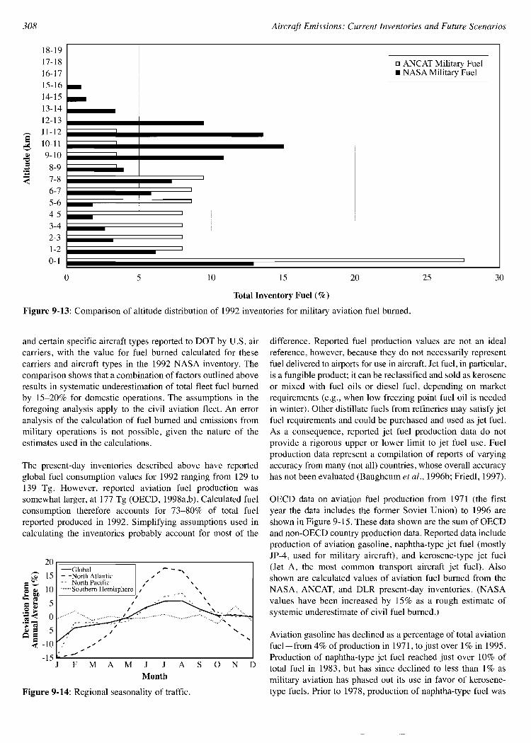
308

18-1917-1816-1715-1614-1513-1412-13

e 11-12

.:.:: 10-11'-'~ 9-10

'C

= 8-9.<::....< 7-8

6-75-64-53-42-31-20-1

Aircraft Emissions: Current Inventories and Future Scenarios

I [] ANCAT Military Fuel I

• NASA Military Fuel

.-..

--o 5 10 15 20 25 30

Total Inventory Fuel (%)

Figure 9-13: Comparison of altitude distribution of 1992 inventories for military aviation fuel burned.

The present-day inventories described above have reportedglobal fuel consumption values for 1992 ranging from 129 to139 Tg. However, reported aviation fuel production wassomewhat larger, at 177 Tg (OECD, 1998a,b). Calculated fuelconsumption therefore accounts for 73-80% of total fuelreported produced in 1992. Simplifying assumptions used incalculating the inventories probably account for most of the

OECD data on aviation fuel production from 1971 (the firstyear the data includes the former Soviet Union) to 1996 areshown in Figure 9-15. These data shown are the sum of OECDand non-OECD country production data. Reported data includeproduction of aviation gasoline, naphtha-type jet fuel (mostlyJP-4, used for military aircraft), and kerosene-type jet fuel(Jet A, the most common transport aircraft jet fuel). Alsoshown are calculated values of aviation fuel burned from theNASA, ANCAT, and DLR present-day inventories. (NASAvalues have been increased by 15% as a rough estimate ofsystemic underestimate of civil fuel burned.)

Aviation gasoline has declined as a percentage of total aviationfuel- from 4% of production in 1971, to just over 1% in 1995.Production of naphtha-type jet fuel reached just over 10% oftotal fuel in 1983, but has since declined to less than 1% asmilitary aviation has phased out its use in favor of kerosene­type fuels. Prior to 1978, production of naphtha-type fuel was

difference. Reported fuel production values are not an idealreference, however, because they do not necessarily representfuel delivered to airports for use in aircraft. Jet fuel, in particular,is a fungible product; it can be reclassified and sold as keroseneor mixed with fuel oils or diesel fuel, depending on marketrequirements (e.g., when low freezing point fuel oil is neededin winter). Other distillate fuels from refineries may satisfy jetfuel requirements and could be purchased and used as jet fuel.As a consequence, reported jet fuel production data do notprovide a rigorous upper or lower limit to jet fuel use. Fuelproduction data represent a compilation of reports of varyingaccuracy from many (not all) countries, whose overall accuracyhas not been evaluated (Baughcum et at., 1996b; Friedl, 1997).

N D

..."- ... ...

aSAMAM J JMonth

Figure 9-14: Regional seasonality of traffic.

and certain specific aircraft types reported to DOT by U.S. aircarriers, with the value for fuel burned calculated for thesecarriers and aircraft types in the 1992 NASA inventory. Thecomparison shows that a combination of factors outlined aboveresults in systematic underestimation of total fleet fuel burnedby 15-20% for domestic operations. The assumptions in theforegoing analysis apply to the civil aviation fleet. An erroranalysis of the calculation of fuel burned and emissions frommilitary operations is not possible, given the nature of theestimates used in the calculations.

20 r;======:;------------,~ 15

6'-' 108~

';;; e 5o ~

~< 0.~ -;~ = -5~=~-1O

-15' --;J F

Aircraft Emissions: Current Inventories and Future Scenarios 309

Table 9-6: Fuel burned and emissions from scheduled air traffic, 1982-92 (DLR).

Fuel NOx CO HC Fuel NOx CO HC[Int'l] [Int'l] [Int'l] [Int'l] [Total] [Total] [Total] [Total]

Year (Tg) (Tg) (Tg) (Tg) (Tg) (Tg) (Tg) (Tg)

1982 19.2 0.31 0.05 0.021983 20.9 0.35 0.06 0.021984 24.7 0041 0.06 0.031985 24.9 0041 0.06 0.021986 26.7 0044 om 0.03 72.2 1.03 0.24 0.101987 30.0 0.51 0.08 0.031988 32.6 0.55 0.09 0.031989 35.8 0.61 0.10 0.03 76.5 1.14 0.27 0.091990 37.2 0.62 0.11 0.041991 36.3 0.59 0.11 0.041992 39.3 0.62 0.10 0.03 93.0 1.31 0.34 0.10

Table 9-7: Analysis of the underestimate offuel burned caused by simplifying assumptions (Baughcum et ai., 1996b).

Changes to Simplifying Assumptions

No winds to actual winds

Standard temperatures to actual temperatures

Combined wind and temperature effects

Payload: increase load factor to 75%

Payload: increase load factor to 75%

Payload: volume limited cargo

No fuel tankering to actual practice

Maximum % Fuel Burned Increase

2.6 (Autumn winds, North Pacific route)

0.7 (Summer temperature, North Pacific route)

3.1 (Autumn winds, ISA+5°C temperature, North Pacific)

0.8 (747-400, North Pacific)

2.5 (737-300, Los Angeles-San Francisco)

7.7 (747-400, North Pacific)

4.0 (737-300, Los Angeles-San Francisco, four leg mission)

not reported as a separate item in the OECD database; it wasincluded in the kerosene-type production data.

The three inventories are in good agreement; given the differentapproaches and data sources used, the inventory results (particularlyfor the present day) are remarkably consistent. Assumptionsregarding the state of NOx reduction technology in 2015 cause thebiggest difference in the results of the three forecasts. The 1992and 2015 inventories of NASA,ANCAT, and DLR are all suitablefor calculating the effects of aircraft emissions on the atmosphere,taking account of differences in the details of the inventories andsystematic underestimates examined above. To correct for thesystematic underestimation of fuel burned in the inventorieswhen calculating the effects of aviation CO2 emissions, fuelburned values for 1992 should be increased by 15% and those for2015 should be increased by 5%, based on the assumption thatinefficiencies in the air traffic control system responsible for extrafuel burned will be much reduced by 2015. A summary of theresults from these inventories is given in Table 9-8. The DLR"trend" inventories (1982-92) include only a portion of total

aviation operations (scheduled international service for all yearsand total scheduled service in 1986, 1989, and 1992); as such, theyare valuable for historical growth analysis and for comparisonswith the NASA and ANCATlEC2 scheduled traffic segments.

9.4. Long-Term Emissions Scenarios

Long-term projections to the year 2050 producing 3-D emissionsdata have been made by the Forecasting and EconomicAnalysis Subgroup of CAEP, using the NASA studies as a base(CAEP/4-FESG, 1998), and by DTI using the ANCAT studiesas a base (Newton and Falk, 1997). Long-term projections oftotal demand, fuel consumption, and emissions (but notproviding 3-D data) have also been made by EDF (Vedanthamand Oppenheimer, 1994, 1998), WWF (Barrett, 1994), and MIT(Schafer and Victor, 1997).

Predictions of traffic demand and resulting emissions beyond2015 become increasingly uncertain because the probability

310 Aircraft Emissions: Current Inventories and Future Scenarios

200

180 -+- Aviation Gasoline---OJ)

E-l -- Naptha-Type Jet Fuel'-'

"Cl 160 -+- Kerosene-Type Jet Fuelcu='"'= -- Total Jet Fueli=CI 140as= ....... All Aviation Fuel~

"Cl 120 • NASA Inventoriescu •....~ A ANCAT Inventories'3~ 100 •-~ • DLR InventoriesU

"Cl 80 .. NASA Inventories + 15%=~=.=: 60....~="Cle 40~-cu=~ 20

0

1960 1966 1972 1978 1984 1990 1996

Year

Figure 9-15: Comparison of calculated fuel burned by aviation with reported production.

for unforeseeable major changes in key factors influencing theresults steadily increases. The best approach for insight into theevolution of long-term futures is the application of scenarios.A scenario is simply a set of assumptions devised to reflect thepossible development of a particular situation over time. Theseassumptions are used as inputs to a model that describes themanner in which an activity might develop over time. A rangeof possible futures can be described by a set of independentscenarios. The results of the scenario are difficult to judge interms of confidence level: They are simply the outcome ofinput assumptions. However, scenarios can be objectivelyjudged as implausible by showing that their assumptions oroutcomes conflict with industry trends or with invariant rulesand laws that might reasonably be expected to remain

unchanged during the scenario time period or by revealinginternal inconsistencies or incompatibilities with other dominatingexternal developments. Investigation of the consequences andimplications of scenarios can be used to support a subjectiveassessment regarding which of the remaining possible scenariosmight be more plausible than others.

9.4.1. FESG 2050 Scenarios

9.4.1.1. Development of Traffic Projection Model

In developing long-term traffic scenarios, various models of trafficdemand were considered (CAEP/4-FESG, 1998), particularly

Table 9-8: Summary comparison ofhistorical, present-day, and 2015 forecast 3-D emissions inventories.

Calculated Calculated Calculated CalculatedInventory Inventory Fuel Burned CO2 (as C) NOx (as N02) Fleet EI(NOx)

Year Source (Tg) (Tg) (Tg) (g N02 kg-t fuel)

1976 NASA 100.0 86.0 1.0 9.81984 NASA 116.3 100.0 1.3 11.01992 NASA 139.4 119.9 1.7 12.01992 ANCAT 131.2 112.9 1.8 13.81992 DLR 129.3 111.2 1.8 13.92015 NASA 308.6 265.4 4.1 13.42015 ANCAT 287.1 246.9 3.5 12.32015 DLR 285.0 245.1 3.6 12.5

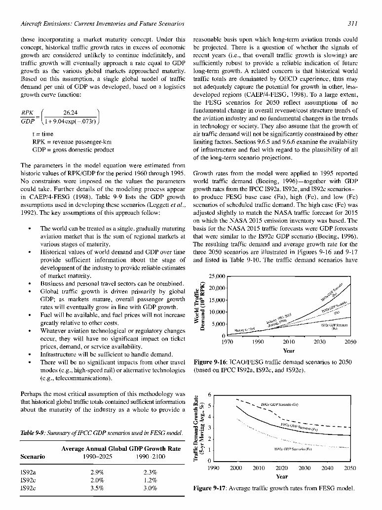
Aircraft Emissions: Current Inventories and Future Scenarios 311

205020302010

Year1990

ol::::=:=:;:=-~____.-~-....__~-__._---.J

1970

Figure 9-16: ICAO/FESG traffic demand scenarios to 2050(based on IPCC IS92a, IS92c, and IS92e).

reasonable basis upon which long-term aviation trends couldbe projected. There is a question of whether the signals ofrecent years (i.e., that overall traffic growth is slowing) aresufficiently robust to provide a reliable indication of futurelong-term growth. A related concern is that historical worldtraffic totals are dominated by OECD experience, thus maynot adequately capture the potential for growth in other, less­developed regions (CAEP/4-FESG, 1998). To a large extent,the FESG scenarios for 2050 reflect assumptions of nofundamental change in overall revenue/cost structure trends ofthe aviation industry and no fundamental changes in the trendsin technology or society. They also assume that the growth ofair traffic demand will not be significantly constrained by otherlimiting factors. Sections 9.6.5 and 9.6.6 examine the availabilityof infrastructure and fuel with regard to the plausibility of allof the long-term scenario projections.

25,000.--------------------,

CJ ~ 20,000ISI:l::~~ 15,000

'-'

:S't:l 10,000"" =~e

~ 5,000I::l

Growth rates from the model were applied to 1995 reportedworld traffic demand (Boeing, 1996)-together with GDPgrowth rates from the IPCC IS92a, IS92e, and IS92c scenarios­to produce FESG base case (Fa), high (Fe), and low (Fc)scenarios of scheduled traffic demand. The high case (Fe) wasadjusted slightly to match the NASA traffic forecast for 2015on which the NASA 2015 emission inventory was based. Thebasis for the NASA 2015 traffic forecasts were GDP forecaststhat were similar to the IS92e GDP scenario (Boeing, 1996).The resulting traffic demand and average growth rate for thethree 2050 scenarios are illustrated in Figures 9-16 and 9-17and listed in Table 9-10. The traffic demand scenarios have

t = timeRPK = revenue passenger-kmGDP = gross domestic product

• The world can be treated as a single, gradually maturingaviation market that is the sum of regional markets atvarious stages of maturity.

• Historical values of world demand and GDP over timeprovide sufficient information about the stage ofdevelopment of the industry to provide reliable estimatesof market maturity.

• Business and personal travel sectors can be combined.• Global traffic growth is driven primarily by global

GDP; as markets mature, overall passenger growthrates will eventually grow in line with GDP growth.

• Fuel will be available, and fuel prices will not increasegreatly relative to other costs.

• Whatever aviation technological or regulatory changesoccur, they will have no significant impact on ticketprices, demand, or service availability.

• Infrastructure will be sufficient to handle demand.• There will be no significant impacts from other travel

modes (e.g., high-speed rail) or alternative technologies(e.g., telecommunications).

RPK ( 2~24 )GDP = 1+ 9.04exp( -.073t)

those incorporating a market maturity concept. Under thisconcept, historical traffic growth rates in excess of economicgrowth are considered unlikely to continue indefinitely, andtraffic growth will eventually approach a rate equal to GDPgrowth as the various global markets approached maturity.Based on this assumption, a single global model of trafficdemand per unit of GDP was developed, based on a logisticsgrowth curve function:

The parameters in the model equation were estimated fromhistoric values of RPK/GDP for the period 1960 through 1995.No constraints were imposed on the values the parameterscould take. Further details of the modeling process appearin CAEP/4-FESG (1998). Table 9-9 lists the GDP growthassumptions used in developing these scenarios (Leggett et al.,1992). The key assumptions of this approach follow:

Table 9-9: Summary ofIPCC GDP scenarios used in FESG model.

205020402030

--..... ... ...

2010 2020

Year

........ .... IS92e GDPScenario (Fe).....

2000

6.-------------------...,

OL..- ...J

1990

Figure 9-17: Average traffic growth rates from FESG model.

2.3%1.2%3.0%

2.9%2.0%3.5%

Average Annual Global GDP Growth Rate1990-2025 1990-2100

Perhaps the most critical assumption of this methodology wasthat historical global traffic totals contained sufficient informationabout the maturity of the industry as a whole to provide a

Scenario

IS92aIS92cIS92e

312 Aircraft Emissions: Current Inventories and Future Scenarios

Table 9-10: Traffic projections and 5-year average growth rates from FESG (CAEP/4 - FESG Report 4, 1998).

Fa Fa Fe Fe Fe FeDemand Growth Rate Demand Growth Rate Demand Growth Rate

Year (109 RPK) (0/0) (109 RPK) (0/0) (109 RPK) (0/0)

1995 2,536.6a 2,536.6a 2,536.6a

2000 3,238.0 5.0 3,068.8 3.9 3,336.1 5.62005 3,981.4 4.2 3,591.9 3.2 4,322.4 5.32010 4,782.6 3.7 4,103.0 2.7 5,491.7 4.92015 5,638.6 3.3 4,596.1 2.3 6,876.2 4.62020 6,552.9 3.1 5,070.7 2.0 8,302.4 3.82025 7,533.6 2.8 5,530.7 1.8 9,908.5 3.62030 8,592.7 2.7 5,981.4 1.6 11,727.0 3.42035 9,744.9 2.5 6,429.8 1.5 13,794.9 3.32040 11,006.8 2.5 6,881.5 1.4 16,155.8 3.22045 12,396.5 2.4 7,342.5 1.3 18,864.2 3.12050 13,933.5 2.4 7,817.2 1.3 21,978.2 3.1

aActual reported traffic for 1995.

been labeled Fa through Fe for brevity; these labels, whencombined with the appropriate technology assumption designator(l or 2; see Section 9.4.1.2), form the complete designator forthe FESG scenarios used throughout the rest of this report.

Global traffic from the model projections was apportioned over45 regional traffic flows with a separate market share modelbecause certain regions grow faster than others, and the correctdistribution of traffic is important in the calculation of theeffects of emissions on the atmosphere. In this procedure,regional traffic flows were expressed as a share of the globalmarket; using the market share and historical growth patternsensures consistency between regional flows and the globalforecast. The underlying assumption of this procedure is thateach regional share approaches its ultimate share of the totalmarket asymptotically. Mature markets tend to have decliningshares approaching an asymptotic value, whereas developingmarkets tend to increase their shares. Adjustments of trafficflows were made so that the "top-down" traffic projections ofthe FESG global model were matched by a reasonable "bottom­up" distribution of regional traffic flows. These traffic flowsinclude all traffic in all regions, and regional variations ingrowth rates are highlighted. Factors that affect the operationsof military and general aviation aircraft were also estimated,and projections were made of the growth of these sectors(CAEP/4-FESG,1998).

9.4.I .2. FESG Technology Projections

Calculations of fuel burned and NOx emissions produced bythe 2050 scheduled fleet were made by applying projections ofoverall improvement in fleet fuel efficiency and emissioncharacteristics to regional traffic flows and summing theresults. These projections were created from technology-levelestimates for new aircraft over time made by a working group

of the International Coordinating Council ofAerospace IndustriesAssociations (ICCAIA) (Sutkus, 1997); they are discussed inSection 7.5.5. A "fleet rollover" model was used to project afleet average fuel efficiency trend, using characteristics of thepresent-day fleet and traffic demand from the FESG scenarios(Greene and Meisenheimer, 1997). The ICCAIA projectionswere made for two technology scenarios. The first scenarioassumes that fuel efficiency and NOxreduction will be consideredin the design of future aircraft in a manner similar to the currentdesign philosophy. The second technology scenario assumes amore aggressive NOx reduction design strategy that will resultin smaller improvements in fuel efficiency. The assumptionsassociated with the two technology scenarios are given inTable 9-11. The basis for projections of aircraft emissionsmade by FESG for the year 2050 was the 3-D NASA emissionsscenarios for the year 2015 discussed in Section 9.3.2. TheNASA 2015 emissions inventory was factored on the basis ofthe product of the ratios of regional traffic (as departures), fleetfuel efficiency, and fleet EI(NOx) as calculated for 2050 overthe same values in 2015. For all flights in a given region:

NOxEmissions2oso = NOxEmissions201s x (regional traffic2osolregional traffiCwlS) x (fleet fuel efficiency20soIfleet fuel efficiencY201S) x (fleet EI(N0x)20soIfleet EI(NOxholS)

Figure 9-18 shows the trend for average new production andfleet average fuel efficiency as a function of time, derived fromICCAIA inputs and the fleet rollover model for the FESG high­demand traffic growth scenario. The average NOx emissionindex for the scheduled fleet over the same time period isshown in Figure 9-19. The 2050 fleet average values used inthe calculation of emissions from scheduled traffic as well asthe baseline 2015 value are given in Table 9-12 (Sutkus, 1997).Fleet fuel efficiency is predicted to improve by about 30%between 2015 and 2050.

Aircraft Emissions: Current Inventories and Future Scenarios 313

Table 9-11: ICCAIA NOx andfuel-efficiency technology assumptions for 2050.

Technology Scenario Fuel Efficiency Increase by 2050 LTO NOx Levels

Design for fuel efficiencyand NOx reduction

Average of production aircraft will be40-50% better relative to 1997 levels

Fleet average will be 10-30% below CAEP/2 limitby 2050; fleet average EI(NOx) = 15.5 in 2050

Design for aggressive NOx

reductionAverage of production aircraft will be30-40% better relative to 1997 levels

Average of production aircraft will be 30-50%below CAEP/2 limit by 2020 and 50-70% belowCAEP/2 limit by 2050; fleet average EI(NOx) =11.5in 2050

Figure 9-18: Fuel efficiency trends to 2050 corresponding tothe two ICCAIA technology scenarios for the FESG hightraffic demand case.

from the base year; these factors were then applied to the 1992ANCAT/EC2 emissions inventory to produce gridded resultsfor the 2050 scenario.

The DTI model relates air traffic demand in RPKs with regionaland global economic performance as reflected in GDP trends,as was the case with the ANCAT/EC2 2015 forecast. Generally,a load factor of 70% is assumed to estimate ASKs (capacity)from traffic demand. Long-term traffic demand is also assumedto be modified by the same assumptions on fares pricing, marketmaturity, and so forth that the ANCAT/EC2 2015 forecastused. Capacity estimates are converted to fuel consumption

2050204020302020Year

I

2010

NASA Projected 2015 Fleel

2000

ICCAJA Scenario 1 New Production~ ,

ICCAIAScenario2NewProduction~ ~-

60 ,------------------:-:1

55....=­~ Q,l

::: ::l 50.~ .....~,....e bJJ 45

f;I;1-"=

Qj~ 40::l~

..... '-0'

3530 L..- - __- __-----l

1990

9.4.1.3. FESG Emissions Scenario Results

Traffic in the FSU and the People's Republic of China has nothistorically been reported in airline schedule databases such asthe OAG. Fuel burned and emissions from aviation in theseregions were estimated individually and projected to 2015(Mortlock and Van Alystyne, 1998), then extended to 2050(CAEP/4-FESG,1998).

Results of calculations of fuel burned and NOx emissions forthe year 2050 based on the long-term scenarios describedabove are given in Table 9-13. The FESG complete scenariosare identified below and in the remainder of this chapter bycombining the demand scenario (e.g., Fa) with the technologyscenario number (e.g., Fal, Fe2).

9.4.2. DTI2050 Scenarios

The DTI projection for air traffic and emiSSIOns for 2050(Newton and Falk, 1997) has been developed from the DTItraffic and fleet forecast demand model, in conjunction withdata from the ANCAT/EC2 inventory. The forecast model wasdeveloped from DTI's global and regional traffic forecastmodels for passenger and freight traffic. Fuel consumptiontrends were estimated with a fleet fuel efficiency model, andfleet emissions performance were estimated on the basis ofassumed regulatory change. Finally, appropriate fuel andemissions factors were calculated to estimate 2050 figures

Table 9-12: Projected scheduledfleet jitel efficiency (Sutkus, 1997).

Scheduled Fleet FuelEfficiency (ASK kg-! Fuel)

1980 1990 2000 2010 2020 2030 2040 2050Year

ICCAIA Scenario 2[Design for Aggressive

NOx Reduction]

ICCAIA Scenario 1[Design for Fuel Efficiency

and NOx Reduction1

- - - - - - - -t20%

NASA 2015 Projedion

Figure 9-19: Fleet average trends in EI(NOx) showingprojections for the two ICCAIA technology scenarios.

16

'6 14~ 12...f;I;1 10

Q,l

: 8"'"Q,l 6<~ 4~ 2.....O~-----------------1970

51.851.452.0

TechnologyScenario 2

41.8

53.653.154.0

TechnologyScenario 1

Demand scenario FaDemand scenario FcDemand scenario Fe

2015 NASA Inventory

Traffic Scenario

314

Table 9-13: Results of FESG year 2050 scenarios calculations.

Aircraft Emissions: Current Inventories and Future Scenarios

Sector Fal Fa2 Fel Fe2 Fel Fe2

Calculated Fuel Burned (Tg)Scheduled 396.1 410.8 224.0 232.3 620.0 643.9Charter 21.4 22.2 12.1 12.6 33.5 34.8FSu/China 30.3 31.4 8.8 9.1 67.5 70.1General Aviation 8.8 8.8 8.8 8.8 8.8 8.8

Civil Subtotal 456.6 473.2 253.8 262.8 729.8 757.7Military 14.4 14.4 14.4 14.4 14.4 14.4

Global Total 471.0 487.6 268.2 277.2 744.3 772.1

Calculated CO2 Emissions (Tg C)Scheduled 340.7 353.3 192.7 199.7 533.2 553.7Charter 18.4 19.1 10.4 10.8 28.8 29.9FSu/China 26.0 27.0 7.5 7.8 58.1 60.3General Aviation 7.6 7.6 7.6 7.6 7.6 7.6

Civil Subtotal 392.7 407.0 218.2 226.0 627.7 651.6Military 12.4 12.4 12.4 12.4 12.4 12.4

Global Total 405.1 419.4 230.6 238.4 640.1 664.0

Calculated NOx Emissions (Tg as N02)

Scheduled 6.1 4.7 3.5 2.7 9.6 7.4Charter 0.4 0.3 0.2 0.2 0.6 0.4FSU/China 0.5 0.3 0.1 0.1 1.0 0.8General Aviation 0.1 0.1 0.1 0.1 0.1 0.1

Civil Subtotal 7.0 5.4 3.9 3.0 11.3 8.7Military 0.1 0.1 0.1 0.1 0.1 0.1

Global Total 7.2 5.5 4.0 3.1 11.4 8.8

Calculated Fleet Average EI(NO) [g NOx (as N02) kg-] fuel burned]Scheduled 15.5 11.5 15.5 11.5 15.5 11.5Charter 16.7 12.4 16.7 12.4 16.8 12.4FSu/China 14.9 11.1 14.9 11.1 14.9 11.0General Aviation 9.0 9.0 9.0 9.0 9.0 9.0

Civil Subtotal 15.4 11.5 15.3 11.4 15.4 11.5Military 8.7 8.7 8.7 8.7 8.7 8.7

Global Total 15.2 11.4 15.0 11.3 15.3 11.4

estimates by using the concept of traffic efficiency as described positive throughout the scenario, but growth rate declinesin Section 9.3.2 and a fuel efficiency trend for the scenario during the period. Decadal capacity growth rates-actual andperiod. Model coverage includes all global aviation markets, forecast-are given in Table 9-14. The traffic forecast includesbut separate fuel consumption estimates are made for freight civil and freight operations as well as civil charter and businessand for the FSU on the basis of aligning growth with global jet traffic but excludes military aviation activity and possiblecivil passenger market trends. future supersonic operations.

The scenario modeled for 2050 assumes that sufficient aviationinfrastructure would be available to accommodate the forecastincrease in traffic. No new city pairs are introduced during thescenario period, and aircraft flight profiles remain unalteredfrom the present day; altitude, speed, and method of operationare assumed to be the same as present-day values, even forlarger aircraft types (600+ seats) that are assumed to enterservice beginning in about 2005. All traffic is assumed to becarried by a subsonic aircraft fleet (i.e., no HSCT would beoperating by 2050). The model forecasts traffic growth to be

Fuel usage was determined for the base year fleet from thecapacity offered in that year (ASKs) and the fleet's trafficefficiency (ASK per kg fuel). A fuel efficiency trend suggestedby Greene (1992) and modified by DTI was included as ascenario parameter, as given in Table 9-15.

The traffic efficiency of the fleet over the scenario period wasestimated to range from 30 ASK kg-! in the base year 1992 to48 ASK kg-! in 2050 (a 60% improvement). This estimate wasbased on the performance of existing aircraft types and forecasts

Aircraft Emissions: Current Inventories and Future Scenarios 315

Table 9-14: Actual and forecast global capacity growth ratesused in the DTl model.

Table 9-16: Trend ofcivil fleet E1(NOx) in DTl projections.

Table 9-15: Assumed annual improvements infuel efficiencyin DTl model.

of the type and number of aircraft (categorized by seat bandand technology level) that might be flying in 2050. Futureaircraft types included size developments to 799 seats.

A major scenario element was the NOx reduction technologyassumption. Current technology will allow engines to achievereductions of around 30% below the current certification level(CAEP/2 standards). The basis of the technology scenario wasthat NOx regulations would be made considerably more stringentthan today and that the manufacturing industry would developappropriate technology solutions. This development was modeledby assuming that from 1992:

• CAEP/2 certification standard applies to all newproduction from 2000

• 30% reduction in ICAO recommended limits fromCAEP/2 in 2005

• 60% reduction from CAEPI2 phased in equally over8 years from 2035.

With a fleet development trend determined by the capacityforecast, the rate of introduction of the scenario above impliesa global fleet emissions index trend that is as compatible withthe relatively modest fuel efficiency assumption given inTable 9-16. The fleet EI(NOx) of 7.0 implies widespread use ofultra-low NOx technology (Section 7.5). The total calculatedfuel burned and emissions for 2050 under the DTI/ANCATscenario are given in Table 9-17.

Year

1994200020102020203020402050

Year

1991-20002001-20102011-20202021-20302031-20402041 on

ASK Annual Global Growth Rate (%)

5.365.164.823.623.012.491.72

Annual Improvement in Fuel Efficiency (%)

1.3 (Greene, 1992)1.3 (Greene, 1992)

1.0 (DT! extrapolation)0.5 (DT! extrapolation)0.5 (DT! extrapolation)0.5 (DT! extrapolation)

Table 9-17: Results ofDTl2050 projections (military operationsnot included).

Year EI(NOx)

1992 11.12010 10.732020 10.432030 10.32040 9.52050 7.0

The EDF model sorts the nations of the world into five economicgroups (see Table 9-18). For each of the five economic groups,the three sectors of civil business passenger, civil personalpassenger, and civil freight are modeled as logistics with

continued growth, and eventual slowdown in growth rateswithout imposing a zero growth-rate ceiling. Growth rates andmarket capacities for different regions of the world werechosen after a review of economic and aviation market historyin industrial nations. The demand model is consistent with thehistory of the U.S. domestic market.

9.43. Environmental Defense Fund Long-Term Scenarios

EDF has produced projections of total traffic demand, fuel use,and emissions through 2100 (Vedantham and Oppenheimer,1994, 1998). The EDF projections use a logistic model tosimulate the stages of demand growth in aviation markets,focusing particularly on demand growth in developing countries(where aviation has only recently become a commonplace travelmode). Two sets of aviation demand scenarios-base-level andhigh-level-describe traffic under each of the six IPCC 1992scenarios (IS92a through IS92f) for global expectations of grossnational product (GNP), population, and emissions (Leggett etal., 1992). Data produced are regional and global totals.

The model logic incorporates the assumption (based on observation)that latent demand in a region previously not served by airlineswill result in an initial period of rapid growth; once an airportnetwork is in place, business and personal habits will incorporatethe new transport option, causing a period of continuing stronggrowth rates. Barring unforeseen developments, the experienceof some OECD nations suggests that aviation demand willeventually reach maturity, and relative growth rates will slowas the market approaches saturation. Continued growth of GNPand population imply continuing, albeit slow, growth indemand, even over the very long term.

EDF uses a logistic model with a time-varying capacity tomodel the dynamics in several sectors of rapid expansion,

TrafficScenario (109 RPK)

DT! 18106

Fuel(Tg)

633.2

NOx

(Tg N02) EI(NOx)

4.45 7.0

3i6 Aircraft Emissions: Current inventories and Future Scenarios

Table 9-18: Definition of regional economic groups in theEDFmodel.

Group Members

1 OECD members, except Japan2 Asian newly industrialized countries (NICs), Japan3 China and the rest of Asia4 Africa, Latin America, Middle East5 Former Soviet Union (FSU) , Eastern Europe

start of market expansion to maturity. The model assumes thatnations that are building their airport infrastructure today maywell attain market maturity faster because they will benefitfrom technological improvements and some fraction of theirpopulace will be more familiar with lifestyle and businesshabits that incorporate aviation. Another region-specificassumption was that markets in the post-Communisteconomies may mature faster because they have undergoneindustrialization.

time-varying market capacities. The civil business passenger andcivil freight sectors experience logistic expansion toward a time­varying capacity level that is proportional to the nation's GNP.

The model assumes that expansion in business travel isaccompanied by expansion in personal travel, which includestourism and leisure visits. Personal travel by air has highincome elasticity, and aviation demand will increase rapidlywhen a poor nation experiences an economic boom and percapita income increases. Depending on the income distribution,there can be significant demand for aviation even in countrieswith very low per capita incomes (Atkinson, 1975). As incomesrise and seat prices (as well as cargo costs) fall, growth inaviation demand will result from the penetration of aviationservices into lower income brackets (Boeing, 1993). The civilpersonal passenger sector experiences logistic expansiontoward a time-varying capacity level proportional to the nation'spopulation (the model does not account for possible feedbackrelationships between GNP and population). The military andgeneral aviation sectors do not experience logistic expansion;both sectors grow nominally, at the same rate as global GNP.The mathematical basis of the model and further details on theassumptions are given by Vedantham and Oppenheimer (1994,1998).

The six IPCC scenarios for GNP and population, combinedwith the two demand sets described above, provide a total of10 demand projections (because the IS92a and IS92b scenariosshare the same GNP and population expectations). Figure 9-20shows five of the global demand scenarios; sharp upswingswhen different regions start expansion are clearly visible.Annotations attached to the curves are shorthand nomenclaturesfor the scenarios used in this report.

Under the IS92a scenario (the IPCC base case), the base­demand level in 2050 is higher than the 1990 level by a factorof 10.7 and has an average annual demand growth rate of4.03% over the 60-year forecast period (forecasts to 2100 aregiven by Vedantham and Oppenheimer, 1998). For the base­demand set, the range of traffic demand expected for differentpopulation and GNP estimates spans a factor of almost 5 in2050; the full range across all 10 scenarios spans a factor ofmore than 20. Assumptions about rates of expansion andmaturity have a sizable impact: The high-demand projectionfor the IS92a scenario in 2050 is 78% higher than the base­demand value.

The 10 demand scenarios produced by the EDF model aresynthesized with expectations for fuel efficiency improvementand changes in emissions indices to produce fuel use, CO2

emissions, and NOx emissions scenarios.

Figure 9-20: EDF global aviation demand projections.

205020402030

IS92a-HlGH(Eah)

2020

Year20102000

O+----~--~--~---~--_--_i

1990

~; 40,000a­o....::; 30,000

§~ 20,000~~

to~ 10,000

~ L.-===:=::::;'~--

Although fuel efficiency has increased steadily over the pastfew decades, improvements in fuel efficiency are becomingless dramatic over time. The technology projections of the EDFmodel use a constant-capacity logistic that extrapolatesGreene's (1992) forecast for a base-case annual increase

EDF's analysis of the history of the U.S. domestic marketconcluded that there was approximately a 70-year period from

The base-demand and high-demand sets include expected startdate for market expansion, market capacity levels, and maturityperiod length. These assumptions for the two demand setsreflect implicit assumptions about diverse social factors,including travel trends in developing countries (Gould, 1996),penetration of future telecommunications technologies, anddevelopment of competing modes of transportation. Assumptionson start dates of aviation market expansion for rapidly developingeconomies, slowly developing economies, and post-Communisteconomies reflect EDF's own assessment of near-termeconomic expectations and were not made in relation to IPCCscenarios. Prior to the start date, demand is assumed to grownominally, at the same rate as global GNP. The base-demandand high-demand sets include assumptions on market capacitylevels based on multiples of 2 (base-demand) and 3 (high­demand) relative to the 1990 demand levels for EconomicGroup 1 (OECD less Japan), because these markets are closestto maturity today.

Aircraft Emissions: Current Inventories and Future Scenarios 3/7

Table 9-19: Excerpt of EDF results-demand,juel use, CO2, % of global CO2, and NOx '

YearIPCC Scenario Factor 1990 2000 2015 2025 2050

IS92a Base (Eab) Demand (l09 RPK) 2,171 3,629 6,115 9,339 23,256Fuel Use (Tg) 179 258 374 544 1,143CO2 (Tg C) 154 222 322 468 983Percentage of Global CO2 2.1% 2.6% 3.8% 6.8%NOx (Tg) 1.96 2.57 3.28 4.42 7.88

IS92a High (Eah) Demand (l09 RPK) 2,171 5,801 9,954 18,332 41,392Fuel Use (Tg) 179 395 610 1,123 2,086CO2 (Tg C) 154 340 525 966 1794Percentage of Global CO2 2.1% 4.1% 7.9% 12.4%NOx (Tg) 1.96 3.92 5.34 9.12 14.39

IS92c Base (Ecb) Demand (l09 RPK) 2,171 3,447 5,337 7,802 16,762Fuel Use (Tg) 179 243 325 455 837CO2 (Tg C) 154 209 280 391 720Percentage of Global CO2 2.1% 2.8% 4.5% 9.6%NOx (Tg) 1.96 2.42 2.85 3.70 5.77

IS92d High (Edh) Demand (109RPK) 2,171 5,729 9,647 17,619 33,655Fuel Use (Tg) 179 390 592 1,082 1,689CO2 (Tg C) 154 336 510 932 1,453Percentage of Global CO2 2.1% 4.5% 10.0% 16.2%NOx (Tg) 1.96 3.88 5.19 8.79 11.64

IS92e High (Eeh) Demand (l09 RPK) 2,171 5,964 10,850 20,202 46,362Fuel Use (Tg) 179 408 668 1,234 2,297CO2 (Tg C) 154 351 574 1,061 1,975Percentage of Global CO2 2.1% 3.9% 7.0% 9.8%NOx (Tg) 1.96 4.05 5.85 10.02 15.84

of 1.3% in fleet-wide fuel efficiency from 1989 to 2010.Significant differences in fuel efficiency exist today acrossregions, and there may be a tendency toward higher fuelefficiency in wealthier regions. The EDF model assumesdifferences in fuel efficiency across economic groups andbuilds projections on the assumption that the technology gapbetween wealthier and poorer nations will close over time.

CO2 emissions climb rapidly after 2015. For the IS92c scenario(which reflects low population and GNP growth) under bothdemand sets, the level of CO2 emissions in 2100 is lower thanthat in 2050, reflecting a successful catch-up effect wherebytechnological improvements have compensated for demandgrowth (Vedantham and Oppenheimer, 1998).

205020402030

IS92e-HIGH(Eeh)

IS92a-HIGH(Eah)

2020

Year20102000

Figure 9-21: EDF CO2 emissions projections.

uOIl 1,600t::,

Mo 1,200U....o~ 800o.~

~ 400 Le.:::::::::::~~:::::::';:::;:::;;"-

Ot-----~--~--~--~--~-____i

1990

The NOx emissions scenarios reflect changes in EI(NOx)

based on a constant-capacity logistic that extrapolates a best­fit approximation to the 1993 NASA numbers for EI(NOx) in1990 and 2015 (Stolarski and Wesoky, 1993). The modeldoes not reflect specific technology choices for fuel efficiencyor changes in EI(NOx), although the fleet EI(NOx) of 6.9that results from the extrapolation is in the ultra-lowtechnology regime. Results for all scenarios are summarizedin Table 9-19.

Figure 9-21 shows CO2 emissions scenarios [which assume aconstant EI(C02) of 3.16]. Under the base IS92a scenario, CO2

emissions grow at an annual rate of 3.2% to reach 983 Tg C in2050-an increase of a factor of 6.6. For all scenarios, projected

Figure 9-22 shows the NOx emissions scenarios; these scenariosincorporate the effects of fuel efficiency improvements as wellas changes in EI(NOx)' For the base-demand IS92a scenario,NOx emissions rise sharply from almost 2 Tg (as N02) in 1990to 7.9 Tg in 2050. Because total NOx emissions are reduced asa result of fuel efficiency improvements and EI(NOx) reduction,technological improvement can compensate for a greaterfraction of demand growth than in the case of CO2 emissions.

Comparing the EDF scenarios for aviation's CO2 emissionsprojections with the IPCC scenarios for total anthropogenicCO2 emissions (including emissions from energy consumptionand deforestation) provides a benchmark measure of theenvironmental importance of the aviation sector. For the base­demand IS92a scenario, aviation's share of global CO2 emissionsrises from its current value of 2.1 % to a level of 3.8% in 2025and 6.8% in 2050. Across all scenarios, aviation's share ofglobal CO2 emissions ranges between 3.3 and 10% in 2025 andbetween 5.6 and 17.6% in 2050. These scenarios imply thataviation may become a significant contributor to global CO2

emissions.

A study of the long-term future mobility of the world populationhas been undertaken at MIT. This study constructed scenariosbased on the simple yet powerful assumption that time spentand share of expenditures on travel remain constant (Zahavi,1981), on average, over time and across regions of the globe(Schafer and Victor, 1997). Stability of average time budgetsfor travel (motorized and nonmotorized) is substantiated by aconsiderable amount of aggregate historical data. Althoughthere is some variability in travel budgets from poorer to richernations, within each society travel budgets have generallyfollowed a predictable pattern-rising with income andmotorization and stabilizing at 10-15%.

With an annual growth rate of 5.2%, demand rises by a factorof more than 12 between 1991 and 2041 in the "business-as­usual" case. Proposed policies, including changes in load factor,and technological improvements result in a forecast for demandincrease of about a factor of 3 in the "demand management"case. Carbon emissions in 2041 constitute 550 Tg C, andaviation's share of global carbon emissions rises to 15% by 2041.

(percentage of total passenger seats that are occupied) couldincrease fuel efficiency per seat-km for aviation. The modelevaluates a wide range of policy and operational choices,including a 100% load factor and a 100% fuel tax.

Aircraft Emissions: Current Inventories and Future Scenarios

The model includes explicit assumptions of fixed growth ratesin leisure travel, business travel, average trip length forpassenger and freight traffic, and freight tonnage. It assumesthat passenger load factors rise to 75% by 2020 in the basecase. Constant rates of improvement are assumed for aircraftsize, airframe efficiency, and EI(NOx)'

9.4.5. Massachusetts Institute of TechnologyLong-Term Scenarios

205020402030

IS92e-HlGH(Eeh) ----..I

IS92a-HIGH(Eah)

2010

318

18

--- 16N

0Z 14OJ)

Eo-< 12'-'

"0 10Z.... 80

'" 6=.S4'".~e 2

f;Iil01990 2000 2020

Year

Figure 9-22: EDF NOx emissions projections.

Table 9-19 presents an excerpt of EDF model results of trafficdemand, fuel burned, and emissions of CO2 and NOx throughthe year 2050 for the several sets of assumptions. The three­letter designators for the EDF scenarios (e.g., Eab, Eeh) areused throughout this report.

Using the constant travel budget hypothesis, Schafer andVictor (1997) produced global passenger mobility scenarios for11 world regions and four transport modes for the period1990-2050. Adding estimates of changes in the energy intensityof transportation modes, they also generated scenarios of CO2

emissions from passenger transport (see Table 9-20).

9.4.4. WorldWide Fundfor Nature Long-Term Scenario

A study by WWF addresses future aviation demand by analyzingload factors and capacity constraints, particularly in the freightmarket (Barrett, 1994). Analysis of historical data shows thatincreases in the number of seats per aircraft have begun to leveloff. The study examines the effects of pollution control strategiessuch as phasing out of air freight and policies to encourageintermodal shifts to road and rail. Technological options forreducing the environmental impact of aviation (such asoperational improvements, changes in cruise altitude andalternative fuel sources) are examined. In particular, thesemodels consider the feasibility that increases in load factors

The high-speed travel category includes aviation, but the aviationportion of high-speed travel is not explicitly characterized.Results of this model projection therefore cannot be useddirectly in evaluations of the effect of aviation on the atmosphere,nor can they be directly compared to other long-term projectionsof emissions from aviation.

9.5. High-Speed Civil Transport (HSCT) Scenarios

The technology for commercial (supersonic) HSCT is beingdeveloped in the United States, Europe, and Japan. The goalis to develop an aircraft that can carry approximately 300passengers, with a 9,260-km range, cruising at Mach 2.0-2.4 at

Aircraft Emissions: Current Inventories and Future Scenarios

altitudes of 18-20 km. As described in Chapter 7, NASA hasan aggressive technology program to develop combustors withNOx emission levels of 5 g NOx (as NOz) per kg fuel burned atsupersonic cruise conditions. The HSCT is expected to flysupersonically only over water because of the need to mitigatesonic booms over populated land masses. The potential marketfor the HSCT is limited by economic and environmentalconsiderations.

9.5.1. Description ofMethods

3-D emissions inventories of fuel burned, NOx ' CO, andunburned HC for fleets of 500 and 1,000 active (high utilization)HSCTs have been developed based on market penetrationmodels and forecasts of air traffic in 2015 (Baughcum et al.,1994; Baughcum and Henderson, 1995, 1998). Although suchlarge fleets clearly will not be in operation by 2015, the yearwas chosen as a base year because detailed industry projectionsof air traffic on a route-by-route basis are available only to thattime period. Although the introduction of an economical HSCTmay stimulate total traffic growth by an unknown amount, theHSCT will certainly displace some traffic from the subsonicfleet on major long-range intercontinental routes. For this study,possible stimulative effects were ignored to reduce the numberof variables, and HSCT-generated RPKs were explicitlysubstituted for subsonic RPKs on a route-by-route basis.

The most recent set of scenarios based on the NASA technologyconcept aircraft (TCA) HSCT were used for most of theatmospheric impact calculations presented in Chapter 4. It isnot clear when HSCT technology will be mature enough forviable commercial service, so fleet sizes and technology levelsare treated parametrically.

319

The projected flight tracks for a fleet of 500 HSCTs above13-km altitude are shown in Figure 9-23. Because of its speedadvantage over subsonic aircraft, the HSCT would likely beused primarily on long intercontinental routes, where thatadvantage can best be utilized. Because of the sonic boom thattrails below the aircraft, the best HSCT routes have a largeportion of the flight path over water. These conditions combineto put a majority of HSCT routes at northern mid-latitudes overthe North Atlantic and North Pacific.

To project the HSCT fleets and their displacement of subsonicaircraft in the scenarios to 2050, the following procedure wasused:

1) 3-D displacement scenarios of subsonic traffic by afleet of 1,000 active HSCTs was calculated for the year2015 using differences in the 3-D scenarios calculatedfor the NASA all-subsonic fleet (Baughcum et al.,1998) and the NASA subsonic fleet in the presence ofan HSCT fleet (Baughcum and Henderson, 1998).

2) This subsonic displacement scenario was then scaledfor the technology growth factors described in thediscussion of the FESG scenario and combined withthe HSCT only-scenario (assuming the TCA technologylevel) and 2050 all-subsonic scenarios.

The 1,000-unit fleet should not be considered a forecast of theactual number of HSCTs that might be in the fleet in 2050.For this sensitivity study, the LOOO-unit value was chosen torepresent a fleet that would be the result of a successful HSCTprogram; this fleet size also was chosen so that previous fleetprojections could be used (Baughcum and Henderson, 1998).No changes in fuel efficiency or NOx emissions technologyrelative to the assumptions used in the reference were assumed

Table 9-20: Results ofMIT reference scenario-passenger travel and carbon emissions.

1990 2050 1990 2050(1012 pkma) (1012 pkm) (1012 mt C) (1012 mt C)

IndustrializedHigh-Speed 1.5 32.7 0.09 0.66Total 12.4 44.4 0.52 1.12

ReformingHigh-Speed 0.3 2.1 0.02 0.04Total 2.3 7.1 0.Q7 0.20

DevelopingHigh-Speed 0.4 7.2 0.02 0.14Total 8.6 53.8 0.18 1.29

WorldHigh-Speed 2.2 42.0 0.13 0.84Total 23.3 105.3 0.77 2.61

Source: Schafer and Victor (1997); additional data supplied by David Victor (June 1998).apkm=passenger kilometers.

320

300 N

Q,l"Cl

= 0::::....~

.....;I

300 S

Aircraft Emissions: Current Inventories and Future Scenarios

,I .4r-.-...J.---....._-_J~."

1800 W 1500 W 1200 W 900 W 600 W 300 W 0 300 E

Longitude

0.0 1.0 2.0 3.0 4.0

logiO Fuel (kg day·I)

5.0 6.0 7.0

Figure 9-23: Flight tracks above 13-km altitude for a fleet of 500 high-speed civil transports (Baughcum and Henderson, 1998).

for the 2050 HSCT. A detailed description of the routesystem flown by the 1,000 HSCTs is given by Baughcum andHenderson (1998).

9.52. Description ofResults

Fleet fuel burned with the HSCT was calculated by assumingthat the fuel efficiency and NOx emissions of the subsonicfleet were described by NOx technology scenario 1, the "fuelefficiency" scenario. Table 9-21 gives the total fleet fuelburned and NOx emissions with and without the assumed1,000-unit HSCT fleet. Fleet fuel burned increases as a resultof the substitution of less fuel efficient HSCTs for subsonicairplanes (present HSCT designs have about half the fuelefficiency, measured as RPK per fuel burned, of present subsonicairplanes). However, fleet NOx emissions decrease in spite ofthe increase in fuel burned because the HSCT is assumed to bedesigned for very low NOx emissions [cruise EI(NOx) of 5].

A comparison of the altitudinal distributions of fuel use andNOx emissions between the all-subsonic fleet and a fleet

containing subsonic and HSCT aircraft is shown in Figures9-24 and 9-25 for the FESG year 2050 IS92a scenario. Theintroduction of an HSCT fleet with EI(NOx)=5 combustorswould be expected to increase emissions above 12-km altitudeand lead to a decrease of NOx emissions below 12, particularlyin the 10-12 km band, assuming that the introduction of anHSCT will cause a displacement of subsonic traffic.

9.6. Evaluation and Assessmentof Long-Term Subsonic Scenarios

9.6.1. Difficulties in Constructing Long-Term Scenarios

Long-term (beyond 20 years) projections of aviation trafficdemand, fleet fuel burned, and fleet emissions are inevitablyspeculative. Difficulty in forecasting technological developmentsthat might be appropriate for the long term, possible shiftsin traffic demand, and myriad uncertainties resulting fromhuman society's development over the period in question allconspire to make long-term projections unreliable-sometimesastoundingly so. Given the state of the aviation industry 50

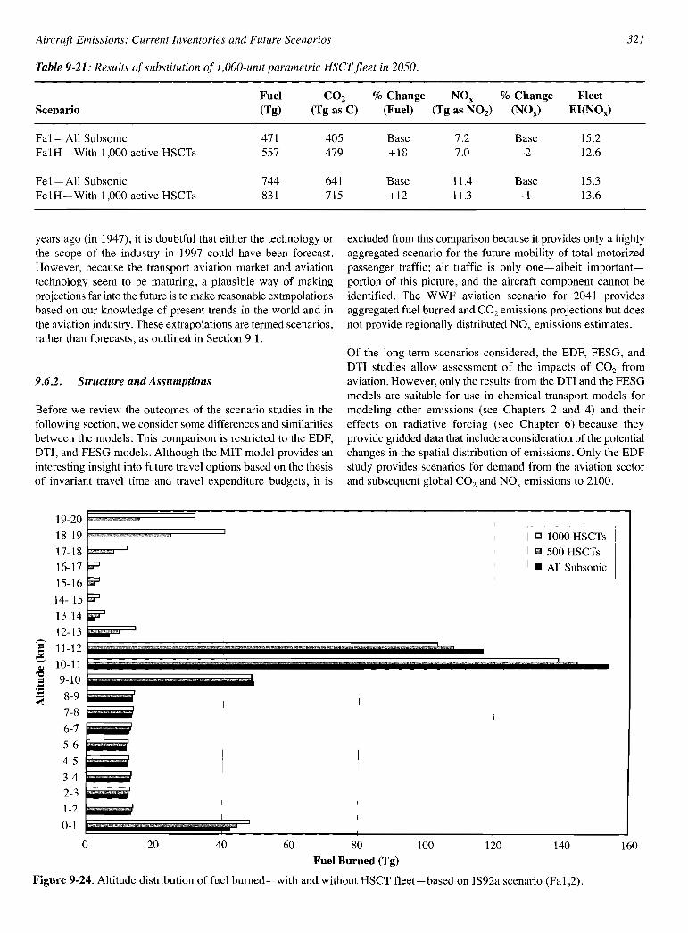
Aircraft Emissions: Current Inventories and Future Scenarios

Table 9-21: Results of substitution of I ,ODD-unit parametric HSCT fleet in 2050.

Fuel CO2 % Change NOx % Change FleetScenario (Tg) (Tg as C) (Fuel) (Tg as N02) (NOx) EI(NOx)

Fa1-All Subsonic 471 405 Base 7.2 Base 15.2Fa1 H - With 1,000 active HSCTs 557 479 +lg 7.0 -2 12.6

Fe1-All Subsonic 744 641 Base 11.4 Base 15.3Fe1H-With 1,000 active HSCTs 831 715 +12 11.3 -1 13.6

321

years ago (in 1947), it is doubtful that either the technology orthe scope of the industry in 1997 could have been forecast.However, because the transport aviation market and aviationtechnology seem to be maturing, a plausible way of makingprojections far into the future is to make reasonable extrapolationsbased on our knowledge of present trends in the world and inthe aviation industry. These extrapolations are termed scenarios,rather than forecasts, as outlined in Section 9.1.

9.6.2. Structure and Assumptions

Before we review the outcomes of the scenario studies in thefollowing section, we consider some differences and similaritiesbetween the models. This comparison is restricted to the EDF,DTI, and FESG models. Although the MIT model provides aninteresting insight into future travel options based on the thesisof invariant travel time and travel expenditure budgets, it is

excluded from this comparison because it provides only a highlyaggregated scenario for the future mobility of total motorizedpassenger traffic; air traffic is only one-albeit important­portion of this picture, and the aircraft component cannot beidentified. The WWF aviation scenario for 2041 providesaggregated fuel burned and CO2 emissions projections but doesnot provide regionally distributed NOx emissions estimates.

Of the long-term scenarios considered, the EDF, FESG, andDTI studies allow assessment of the impacts of CO2 fromaviation. However, only the results from the DTI and the FESGmodels are suitable for use in chemical transport models formodeling other emissions (see Chapters 2 and 4) and theireffects on radiative forcing (see Chapter 6) because theyprovide gridded data that include a consideration of the potentialchanges in the spatial distribution of emissions. Only the EDFstudy provides scenarios for demand from the aviation sectorand subsequent global CO2 and NOx emissions to 2100.

19-20

18-1917-1816-17

15-16

14- 1513-14

12-13

~ 11-12<l.l 10-11

~ 9-10~ 8-9

7-8

6-75-6

4-5

3-42-3

1-20-1

I

II

I II o 1000 HSCTs

-- II III 500 HSCTs

I

;.;;::JI I • All Subsonic

iii? II I

iii? I I I

i? I II

I II-- I II

,

II

i

I i

I

I I

I II

I

o W ~ ~ W 100 lW 1~ 1~

Fuel Burned (Tg)

Figure 9-24: Altitude distribution of fuel burned-with and without HSCT fleet-based on IS92a scenario (Fa1,2).

322 Aircraft Emissions: Current Inventories and Future Scenarios

2.5

I

I

21.51

I

I

I

I

0.5o

19-20f;~;;::::::i""----TI-------------------:-------'

18-19~ [J 1000 HSCTs17-18 ~ III 500 HSCTs16-17 iI • All Subsonic

15-16 ~

14-15 iI

13-14,12-13 Iiiiiii'?

QJ 10-11

~ 9-10

~ 8-97-8

6-7

5-6

4-5

3-4

2-3

1-2

0-1

NOx Emissions (Tg)

Figure 9-25: Altitude distribution of NOx emissions-with and without HSCT fleet-based on IS92a scenario (Fal, FaH).

The EDF study provided 10 scenarios based on five differentIPCC IS92 world scenarios for the long-term development ofworld economy and population and two air traffic demandscenarios (base case and high case). The FESG study calculatedthree air traffic demand scenarios based on the IPCC IS92a,IS92c, and IS92e world scenarios, which were combined withtwo engine technology scenarios to produce six differentemissions inventories.

The FESG scenarios of regional and global air traffic werebased on a logistic regression model of traffic demand since1960 using global GDP as a predictor. The FESG model useda combination of top-down and bottom-up approaches, in whichglobal volumes of civil aircraft flight kilometers were predictedusing the regression model for different GDP scenarios. Allavailable information on regions, including regional variationin growth, was then used to disaggregate these global values ina consistent way over 45 traffic flows within and between theregions of the world by using a market share allocation model.Year 2050 values of fuel burned and NOx emissions for militarytraffic were estimated separately.

The EDF scenarios also were based on the use of logisticgrowth curves to model air traffic growth for business andpersonal travel (plus military and freight traffic). Modelparameters were chosen through observation of historicaltraffic trends in the United States. Regional population wasused as a predictor of personal passenger travel, and regionalGNP was used as a predictor of business passenger travel and

freight demand. Both the FESG and EDF models incorporatethe underlying assumption that the chosen parameters aresatisfactory predictors of aviation demand and that aviationmarkets eventually mature.

There are large differences between the EDF and FESG modelswith respect to the development of emissions scenarios. TheEDF model uses a constant capacity logistic to describe fuelefficiency improvements, which extrapolates Greene's (1992)forecast to 2010 with varied rates for five geographic worldregions and the military/freight aviation sector. For the trend infleet EI(NOx) a single global logistic model extrapolatesfrom the 1990 and 2015 values. The FESG scenarios arebased on two engine technology scenarios developed byICCAIA for ICAO/FESG and IPCC (see Chapter 7). Thesescenarios represent an industry perspective on likely futuredevelopments in fuel efficiency and NOx reduction technologies,as well as further potentials and limitations. The fuel efficiencytechnology element of the DTI scenario was similar in thisrespect, but a NOx technology scenario appropriate to stricteremissions regulations was assumed, in which subsonic engineresearch programs would deliver emissions levels similar tothose targeted in the NASA HSCT program.

Additional assumptions are also important to the results of thescenario models. In the EDF model, assumptions about the datesof market expansion and maturity and the ultimate capacitylevels chosen for the economic regions strongly influence theoutcomes.

323

50,000

---~~ 40,000~

0....:; 30,000

==8 20,000...Q~e 10,000=

I~

0"". "1. "1. f:: ~ ~ ~ ..c: ~ ..c: ~ ..c:- - - " () ()

""" """ Jl '"" ()

~Ci ~ ~ ~ ~ ~ ~ ~

p;.. p;..

None of the 3-D gridded inventories for 2050 assume anychanges in design that would alter the cruise altitudes of subsonicaircraft. Furthermore, no consideration was given in any of the2050 scenarios reported here to the possible stimulative (or Figure 9-26: Comparison of traffic demand in 2050.otherwise) effect of HSCT introductions on traffic.

Aircraft Emissions: Current Inventories and Future Scenarios

The EDF, FESG, and DTI models all use statistics of traffic/airtraffic from international organizations and GECD countries,as well as numerous other recently published sources, andadopt one or more of the IPCC IS92 scenarios to describe thelong-term development of worldwide economic growth andpopulation. The FESG, EDF, and DTI models also useinformation from the NASA and ANCATIEC gridded inventoriesof traffic flows and related emissions. The FESG models usednew, partly proprietary, information from industry as a base toproject emissions in the year 2050.

9.63. Traffic Demandpassenger, freight, and business jet traffic but excludes militaryoperations. The WWF model includes passenger and freightonly, but a demand value for 2041 was not published.

Total traffic demand projected for the year 2050 for three of thelong-range scenarios is shown in Figure 9-26. The valuesshown for the FESG model projection do not include militaryor general aviation traffic. Military and general aviation fuelburned and emissions were estimated separately for the year2050; they were 3.1 and 1.8% of total fuel burned, respectively(Fal ,2). The demand values shown for the EDF model includemilitary as well as freight demand, with projected billiontonne-km values converted to RPK. The DTI model includes

Although the FESG and EDF models use the same IS92economic scenarios (IS92 population scenarios also are inputsto the EDF model), the traffic demand projections for 2050from the EDF model are higher than those of the FESG modelby a factor of 1.2 to almost 4, depending on the scenario. TheDTI model, which does not directly depend on the IS92scenarios, projects a traffic demand about 80% that of theFESG high case (Fel,2).

80001990 2050

EDF Passenger - Tourist7000 • EDF Passenger - Business

D FESG Total Passenger

6000---'"~~I:z:: 5000""0....'-''C= 4000=8...Q~ 3000

!5=~

2000

1000

0~C ~:c Q§ en -= +.;:1 S~ ::JV ~C ~ ..... Q § en -= +.;:1 ...... ::JvQro QbJ) Uro ro en C/lo.. Qro Q"fo Uro ro en S ~ C/lo..Uo.. ..... 0..

~::8Uo.. ..... 0..

~:E I..l.l'~ I..l.l ro Z~ -=<J:: ~~ ~::=l I..l.l'~ I..l.lro Z~ -=<J:: <J::1..l.l ~8

~ &: 0""" :E~~ ~

~ 0""" :E<.H ·v ~

en s::: en U.:; I..l.l ~ en -= en u':; ~::a I..l.l...... en·~E .....l

~ 3en .~~

£l ~ en ~ en .....l:-g ~<J::o.. v ci ';;:0.. vE8 0:: () E8 0:: i3::8

.~

<I:: .~

<I::<J:: <J::

Figure 9-27: Comparison of 1990 and 2050 regional demand values based on EDF and FESG models (IS92a scenario).

324 Aircraft Emissions: Current Inventories and Future Scenarios

Table 9-22: Comparison of FESG and EDF model results for year 2050 based on IS92a.

1990 % 1990 % 1990 1990 2050 % 2050 % 2050 2050World World FESG% EDF% World World FESG% EDF%

Region GNP Population Demand Demand GNP Population Demand Demand

I)OECD, less Japan 57 12 63 62 45 8 55 15

2)Asian NICs + Japan 16 3 13 5 13 2 21 4

3)China, Rest of Asia 6 52 2 5 15 49 12 45

4) Africa, Latin America,Middle East 9 25 10 14 18 37 9 30

5)FSU, Eastern Europe 12 7 11 14 9 5 3 6

Clues to the reasons behind the large differences in projectedtraffic demand between the FESG and EDF models can befound by examining the details of the results of each model.The EDF model projects passenger business and personal trafficin five world regions, plus military and freight traffic. To makecomparisons between the two models, the 45 traffic demandflows (allocated from the global growth projection) in theFESG model were assigned to the five regions used in the EDFmodel. Demand flows between two of the EDF-definedregions were allocated by assigning 50% of the FESG trafficdemand to each region.

On the previous page, Figure 9-27 shows a comparison of trafficdemand in 1990 and 2050 from the FESG and EDF models,with demand sorted by region and/or type. The EDF base casedemand (Eab) is compared with the Fal,2 demand scenario.Large differences in the distribution of demand between thetwo models are apparent: The FESG model assigns the largestshare of passenger traffic in 2050 to the OECD area, whereasthe EDF model assigns the largest share to the China-Africaarea (with personal travel making up the bulk of the demand).

Table 9-22 provides data on passenger demand from the EDFand FESG models by region in 1990 and 2050 and regional

14000~ FSU,E.Europe

'"-~ 12000 Africa, Lat.Am., M.E.

Cl<1:l. ,•••••• China, Rest ofAsiaOll~ - - Asian NICs plus Japan

E=-- 10000 - OECD less Japan"'C"' ....C':l'.-' 8000I:l.-=Cl< =~e 6000

C':l Cl<'3~ 4000e ~=1::U'; 2000~ OL..-- -~--_--...J

1990 2000 2010 2020 2030 2040 2050Year

Figure 9-28: Cumulative traffic demand (lS92a scenario, Fal ,2).

distribution of world GNP and population over the same timeperiods. The basis of both models in this comparison is theIS92a GNP and population scenario. In 1990, the demanddistributions of both models are roughly the same and reflectto a great extent the regional distribution of GNP. In 2050, theregional demand distribution from the FESG model reflects theshift in GNP distribution, demonstrating the economics-drivenbasis of the FESG model. The 2050 FESG values also showthat the market share tool has probably underestimated theshare of demand in region 4; percentage of GNP has increasedfrom 1990 to 2050, but percentage of demand has decreased.

In contrast, the 2050 demand distribution from the EDF modeldiffers greatly from the distribution of GNP in 2050 andreflects the population-driven basis of much of the EDF model.

The differences between the FESG and EDF models are furtherillustrated in Figures 9-28 and 9-29, which show the cumulativedistribution of traffic growth over time for the IS92a scenario.Figure 9-28 shows the growth and regional proportions of trafficdemand as projected by the FESG model. The shares of demandreflect the GDP of each region. Figure 9-29 shows the cumulativedistribution of demand for the five regions as projected by theEDF model. The EDF model, unlike the FESG model, projectsbusiness and personal passenger demand separately (businessdemand is a function of GNP; personal demand is a function ofpopulation); both sectors of demand are shown in the figure.Notable is the lack of projected growth in personal demand inregion 1 (OECD less Japan). Driven by projected slow growthand eventual decline in OECD population, demand growth inthis sector is projected to be less than 1% per year after 2005and negative after 2035. Notable also is the relative lack ofgrowth projected for region 2 (Asian newly industrializedcountries + Japan). The effect of the population-driven personaldemand sector is shown by the rapid growth in regions 3(China + rest of Asia) and 4 (Africa, Latin America, MiddleEast). Personal demand in these two regions is projected bythe EDF model to grow at rates exceeding 12% per year for25 years (region 3) and 10% per year for 20 years (region 4) tocreate 75% of total passenger demand in 2050 (up from 19% in

Aircraft Emissions: Current Inventories and Future Scenarios 325

.............. FSU, E. Europe (Business)

-"-'.- FSU, E. Europe (Tourist)...... "' .... .... Africa, Lat.Am., M.E. (Business)

- - -- Africa, Lat.Am., M.E. (Tourist)

China, Rest of Asia (Business).•..•..•..•..• China, Rest of Asia (Tourist)

.•.••.••..•..• Asian NICs plus Japan (Business)

••.••.••.••.•• Asian NICs plus Japan (Tourist)

- - - - - OECD less Japan (Business)OECD less Japan (Tourist)

205020402030

., ........'.'.'.'.'.'.'.'

.......................'.'.'.'.'.'.'

202020102000

18000

16000

~

'"~ 14000~~~=,...;'-''C 12000=~e~

~10000~

IE~

~

'"' 8000~OJ)

'C

=~'"'"~ 6000~~~

~,.:g= 4000e=u

2000

0

1990

Year

Figure 9-29: Distribution of passenger demand (IS92a scenario, Eab).

1990). This value contrasts with the 21% of total passengerdemand projected for these two regions in the FESG model,based on the two regions' 33% share of GNP.

9.6.4. NOx Technology Projections

A list of NOx emissions index projections is given in Table 9-23for the three long-term models (lS92a scenarios).

technology that would produce engine emISSiOns indicesappropriate to those anticipated for staged combustor andultra-low NOx combustor technology-the latter of the typebeing developed for HSCT applications [EI(NOx) =5]. Ultra­low NOx technology concepts now being developed may notbe suitable for future high pressure ratio subsonic enginedesigns, so achieving fleet NOx emission levels assumed inthe DTI and EDF models may be very difficult (see Section7.5).

Table 9-23: Comparison offleet EI(NOxJjrom technologyprojections to 2050.

The EDF model used a logistic extrapolation of NOx trendsfrom NASA work (Stolarski and Wesoky, 1993), but nochanges in technology were explicitly specified.

The fleet EI(NOx) in 1992 was calculated as 12.0 (NASA),13.8 (ANCAT/EC2), and 13.9 (DLR).

Expectations for the development of NOx technology arequite different among the models. The two FESG model NOxtechnology estimates were based on ICCAIA technologyprojections for new aircraft (Sutkus, 1997) and estimates ofhow quickly such new technology would enter the fleet(Greene and Meisenheimer, 1997). The assumptions in theDTI model were that regulatory pressures would requirereductions in NOx emissions, and the fleet emissions indexwould be forced down as the engine industry responded withspecific technology developments through 2035. Thesedevelopments assumed the introduction of emission control

Scenario

FalFa2DTIEab

Fleet EI(NOx)

15.511.57.06.9

326

9.6.5. Infrastructure and Fuel Availability Assumptions

All of the long-term scenarios reviewed in this chapter weredeveloped with the implicit assumption that sufficient systeminfrastructure and capacity will be available to handle thedemand in an unconstrained fashion (infrastructure and capacityare defined for airports as runways, terminals, gates and aprons,roads, etc., and for airways as air navigation services, air trafficcontrol, etc.). However, lack of infrastructure developmentmay well impede future aviation growth. Lack of infrastructurewill result in congestion and delay, additional fuel burn (in theair and on the ground), higher operating costs, higher ticketprices, and reduced service.

In some parts of the world, particularly in North America andEurope, the airway and airports system is currently operatingunder constraints that limit its ability to provide service.These constraints are likely to become more acute in thefuture as the demand for aviation services continues to grow.Congestion resulting from capacity constraints impairs theeconomic and environmental performance of airlines and theentire aviation system. To accommodate future demand,physical and technological infrastructure must be upgradedand expanded. In many areas, however, strong localpressures (especially related to noise created by aircraftmovements) have constrained development of new airportsand capacity improvements at existing airports. It is thereforeimportant to note that the traffic forecasts reviewed in thischapter are all unconstrained forecasts that do not evaluatesystem capacity constraints when estimating future trafficgrowth.

Aviation also depends on petroleum fuels. For the past 50years, known reserves of petroleum have continued toexpand to satisfy 20-30 years of predicted demand. Overthe short-term future, little change in the demand/supplysituation is expected. Oil companies predict continued supplyof their raw material, and kerosene supplies should havesimilar availability as the present day. Despite the forecastfor increasing demand, oil prices are projected to rise onlymoderately over the next 20 years (Hutzler and Andersen,1997). Over the period of these scenarios (to 2050), estimatesof availability are less clear, but there is a general view thatthe oil industry will continue to meet demand (Rogner,1997). There are, however, less optimistic views for oilproduction, with some predictions of a production declineoccurring within the next decade (Campbell and Laherrere,1998). The long-term scenarios assessed for this reportimplicitly assume continued availability of fuel at moderateprices. This is a key assumption for all scenarios becauselarge increases in the price of fuel and/or shortages in supplywould act to restrain demand for passenger and cargo airtransport.

All of the scenarios ignore (in their baseline assumptions)possible changes in service patterns or infrastructure that afuture HSCT might require. The effects of an HSCT fleet areconsidered in Section 9.5.

Aircraft Emissions: Current Inventories and Future Scenarios

9.6.6. Plausibility Checks

Although none of the long-term scenarios reviewed here isconsidered impossible, some may be more plausible thanothers. We devised three simple checks to assess plausibility.The first estimated the fleet size required to carry projectedtraffic in 2050; the second examined implications for airportand infrastructure; and the third examined implications forkerosene demand. These plausibility checks represent an initialexamination of the implications of the scenarios and areintended to illustrate possible consequences of traffic estimatesresulting from the different scenarios. It must be emphasizedthat the fleet numbers produced by this analysis are approximateand are provided for comparative purposes only.

9.6.6.1. Fleet Size

The fleet sizes implied by five of the scenarios were determinedfrom the DTI traffic and fleet forecast model (see Section 9.3.2),which was developed primarily to project demand for newaircraft implied by 25-year traffic forecasts. The DTI modelrequires an annual traffic growth rate as an input; for thisassessment purpose, this value was assumed to be a constantannual rate calculated from the base year traffic and themodel's projection for 2050. The model assumes the fleet tocomprise a range of jet aircraft types, described by seat capacityas follows: 80-99, 100-124, 125-159, 160-199, 200-249,250-314, 315-399,4~99, 500-624, and 625-799. The largeraircraft sizes have yet to be produced but are assumed to enterservice beginning about 2005. Regional variations in fleetcomposition are reflected in the global fleet, based on currenttrends. This analysis does not capture the effects of compositionalchange that could be created as new markets develop. Averageaircraft size growth is assumed (reflecting the historical trendof greater seating capacity for individual aircraft types overtime). The future fleet required to satisfy the scenario demandestimates is derived through an iterative process by matchingcapacity to traffic demand, based on assumptions regardingaircraft unit productivity in capacity terms. Other modelassumptions are as follows:

• Subsonic aircraft supply-projected demand (no supersonics)• A short- and long-haul market share• Future market functions as does the present day (i.e., no

assumptions regarding wider deregulation are made)• Unconstrained demand• Aircraft retired at an average age of 25 years (reduced

productivity from 20-30 years)• Aircraft productivity to improve by an average of 0.75%

annually.

The assumption regarding lack of constraints requires comment.Today's civil aviation market is constrained only by the practicallimitations of airport capacity and access restrictions, airspacerestrictions, and economic restraint resulting from taxation,charges, and so forth that affect ticket price. Any constraints inthe future, whether to address environmental problems or as a

328 Aircraft Emissions: Current Inventories and Future Scenarios

Table 9-27: Required yearly delivery rates ofaircraft impliedby scenarios.

deliveries has followed a generally increasing trend since themid-1950s, and this trend must continue over the scenario periodto satisfy predicted demand for new and replacement aircraft.For the demand cases examined above, deliveries of new aircraftare estimated to reflect the schedule given in Table 9-27.

Total Aircraft Deliveries (in these years)Eab Eeh Fa1,2 DTI

the lowest growth case. Conversely, the highest growth casewould require more than 1,300 new airports of 15 gates each(two new airports per month for 60 years) even if all 3,750airports now listed in the OAG had 15 gates and were capableof handling large jet transport aircraft (which they do not andare not). This analysis ignores infrastructure location and theproblems associated with its provision. In populous parts of theworld, where civil aviation is established, the addition of airportcapacity is often difficult given local environmental pressuressuch developments create. However, in developing countries,where much of the future traffic growth is anticipated, newinfrastructure might encounter less environmental sensitivityand therefore be more readily provided. Nonetheless, theinfrastructure projects required to satisfy the highest growthscenarios are unprecedented in scope.

9.6.6.3. Fuel Availability

Year

2020203020402050

1,1061,0721,5661,714

1,6671,9333,0583,831

813686931948

1,012945

1,3541,440

All of the 2050 scenarios imply large increases in fuel consumptionby aircraft. In the highest FESG scenario (Fe2), aircraft fuelconsumption increases from 139 to 772 Tg yr- 1 over the period1992 to 2050. In the highest EDF scenario (Eeh) , the increaseis from 179 Tg yr-1 in 1990 to 2,297 Tg yr-1 in 2050. Becauseboth scenarios are based on the IS92e scenario, it is appropriateto compare these figures to total energy use in the IS92escenario. According to scenario Fe2, aircraft will account for13% of the total transportation energy usage in 2050 andrequire 15% of the world's liquid fossil fuel production. TheEDF scenario (Eeh) implies that aircraft account for 39% of thetransportation energy usage and require 45% of the world'sliquid fuel production. These comparisons assume that aircraftdo not use biomass fuels or fuels derived from natural gas.

Under either scenario, the world will be straining the limits ofconventional oil resources by 2050. Total remaining resourcesof conventional petroleum, discovered and undiscovered, havebeen estimated at between one trillion (Campbell and Laherrere,1998) and two trillion barrels (Masters et al., 1994-based onthe optimistic 5% probability estimate of undiscovered oil).The IS92e scenario implies cumulative production of liquidfuels of 1 trillion barrels by 2025 and 2 trillion barrels by 2050.Cumulative consumption by 2050 by aircraft alone amounts to0.15 trillion barrels in the Fe2 scenario and 0.35 trillion barrelsin the Eeh scenario. However, production of liquid fuels is notnecessarily limited by conventional oil resources. Liquid fuelscan be produced from heavy oil, tar sands, oil shale, or evencoal, albeit with significantly greater environmental consequencesand at higher costs. High fuel prices would violate the explicitassumptions used in developing the scenarios.

The delivery rate for the Fa1 and Fa2 scenarios would beachievable with existing manufacturing capacity. The deliveryrate required by the highest scenario, Eeh, implies a considerableincrease in manufacturing capacity-approximately six timesthat existing today. Although this level is not impossible, suchan expansion of aircraft manufacturing capability is likely tobe difficult to achieve and sustain during the period. The Eabscenario implies a delivery rate that is approximately threetimes the level existing today, which is not implausible for 2050.

One assumption intrinsic to the fleet size analysis was that theaverage number of seats per aircraft will increase by 1% eachyear, reflecting current trends. This assumption has a largeeffect on fleet size estimates, particularly for high-demand cases.As a sensitivity analysis, the factor was changed to 2% per yearfor the Eeh high scenario and for the Fal and Fa2 scenarios.Such a change may reflect potential market pressures for largeraircraft, which is not inappropriate for a high traffic growthscenario. The results are given in Table 9-28.

As this analysis shows, a different assumption in aircraft sizegrowth has a significant effect on the estimated future fleet.The projected numbers of the largest aircraft types (between625 and 799 seats) in future fleets are particularly sensitive inthis analysis, which suggests that there might be more than7,000 such aircraft in the fleet by 2050 in the Eeh scenario(compared with about 10,000 passenger aircraft of all sizestoday) or about 4,000 additional aircraft for the more conservativeFa1 and Fa2 scenarios.

Increased capacity can be supplied by additional aircraft,increased flying hours (i.e., more efficient use of the fleet),

Table 9-28: Sensitivity offleet size to aircraft capacity.

Fleet at 2050 - Total Aircraft1% yr-1 2% yr- 1

9.6.6.4. Manufacturing Capabilityand Trends in Aircraft Capacity

In 1997, the global aircraft manufacturing capability delivered634 passenger jet aircraft, bringing the global jet passengerfleet to approximately 10,000 aircraft. The rate of new aircraft

Aircraft SizeGrowth Assumption

Eeh scenarioFa1,2 scenario

69,27521,209

42,44811 ,913

Aircraft Emissions: Current Inventories and Future Scenarios 329

Table 9-29: Summary data from long-term scenarios.

Traffic Calculated Calculated Calculated CalculatedScenario Scenario Demand Fuel Burned CO2 (as C) NOx (as N02) Fleet EI(NOx)

Year Name (109 RPK) (Tg yr-l) (Tg yr-1) (Tg yr-1) (g NOikg fuel)

2041 WWF nla 639.5a 550.0 nla nla2050 Fal 13,934 471.0 405.1 7.2 15.22050 FalH 13,934 557.0 479.0 7.0 12.62050 Fa2 13,934 487.6 419.4 5.5 11.42050 Fel 7,817 268.2 230.6 4.0 15.02050 Fc2 7,817 277.2 238.4 3.1 11.32050 Fel 21,978 744.3 640.1 11.4 15.32050 FelH 21,978 831.0 714.7 11.3 13.62050 Fe2 21,978 772.1 664.0 8.8 11.42050 Eab 23,257 1,143.0 983.0 7.9 6.92050 Eah 41,392 2,086.0 1,794.0 14.4 6.92050 Ecb 16,762 837.0 720.0 5.8 6.92050 Ech 29,934 1,528.0 1,314.1 10.5 6.92050 Edb 19,555 959.0 824.8 6.6 6.92050 Edh 33,655 1,689.4 1,452.8 11.6 6.92050 Eeb 26,886 1,298.0 1,116.3 9.0 6.92050 Eeh 46,363 2,297.0 1,975.4 15.8 6.92050 DTI 18,106 633.2 544.6 4.5 7.02050 MIT n/ab 977.0a 840.0b nla nla

aFuel burned calculated from published CO2 data.bContains unspecified fraction from high-speed rail.

larger aircraft, or a combination of these factors. The highaircraft growth assumption used as a sensitivity analysis heresuggests that about 70% of future capacity growth will besupplied by an increase in aircraft size. Although such anindustry trend is not impossible, it is unlikely to occur insuch a prescriptive manner if the industry remains relativelyderegulated. Deregulation tends to favor increased frequencyand direct flights with smaller aircraft between departureand destination. However, it is likely that some markets wouldfavor the proliferation of very large aircraft, especiallythose with dense traffic flows. The size of the fleetssuggested by the 2% per year aircraft size growth assumptionmust therefore be regarded as toward the low end of therange.

9.6.6.5. Synthesis of Plausibility Analyses

Given the range of estimates for traffic, fuel consumption, andemissions from the 2050 aircraft scenarios available to thisassessment, it is necessary to comment on the plausibility of theresults-not least to demonstrate that results used in subsequentanalyses are bounded by sensible limits within which the aviationindustry is currently envisaged to develop.

The foregoing analyses suggest that although none of thescenarios considered for 2050 is impossible, some of the high­growth scenarios (e.g., Eah and Eeh) are probably less plausible.The fleet size and infrastructure implications suggest radical

developments that are likely to be beyond the scope of changesobserved in the industry thus far (or anticipated for the future).Similarly, the low-growth scenarios-though plausible interms of achievability - give traffic estimates that are likely tobe exceeded given the present state of the industry and planneddevelopments. Although all of the FESG scenarios discount thepossibility of truly radical developments in technology over thenext 50 years, they are considered to fall within a plausiblerange of outcomes and suggest achievable developments forthe industry.

The 3-D gridded output from scenarios Fa-Fe (with T1 and T2technology scenarios) and from DTI are suitable for use asinput to chemical transport models and may be used to calculatethe effect of aviation CO2 emissions. Scenarios Eab and Edhare suitable for use in Chapter 6 to calculate the effect of CO2

emissions as sensitivity analyses because the latter scenarioprojects CO2 emissions levels from aviation that are 2.2 timesgreater in 2050 than the highest of the FESG scenarios. Table 9-29provides a summary of all of the long-term scenarios examinedin the chapter.

References

ANCATIEC, 1995: A Global Inventory ofAircraft NOx Emissions. A first version(April 1994) prepared for the AERONOX programme. Abatement ofNuisances Caused by Air Transport (ANCAT) and European CommunityWorking Group, European Civil Aviation Conference, London, UnitedKingdom, 20 pp.

330

Albritton, D.L, G.T. Amanatidis, G. Angeletti, J. Crayston, D.H. Lister, M.McFarland, J.M. Miller,A.R. Ravishankara, N. Sabogal, N. Sundararaman,and HL. Wesoky, 1997: Global Atmmpheric Effects ofAviation: Report ofthe Proceedings ofthe Symposium. NASA-CP-3351, National Aeronauticsand Space Administration, Washington, DC, USA, 52 pp.

Atkinson, A.B., 1975: The Economics of Inequality. Clarendon Press, Oxford,United Kingdom, pp. 22, 246.

Balashov, B. andA. Smith, 1992: ICAO analyses-trends in fuel consumptionby world's airlines. ICAO Journal, 47(8), 18-21.

Barrett, M., 1994: Pollution Control Strategies for Aircraft. World Wide Fundfor Nature, Gland, Switzerland, 60 pp.

Bauer, E., 1979: A catalog of perturbing influences on stratospheric ozone,1955-1975. Journal of Geophysical Research, 84,6929--6940.

Baughcum, S.L., S.c. Henderson, P.S. Hertel, D.R. Maggiora, and C.A.Oncina, 1994: Stratospheric Emissions Effects Database Development.NASA-CR-4592, National Aeronautics and Space Administration,Langley Research Center, Hampton, VA, USA, 156 pp.

Baughcum, S.L., and S.C. Henderson, 1995: Aircraft Emission InventoriesProjected in Year 2015 for a High Speed Civil Transport (HSCT)Universal Airline Network. NASA-CR-4659, National Aeronautics andSpace Administration, Langley Research Center, Hampton, VA, USA,117 pp.

Baughcum, SL., S.c. Henderson, and T.G. Tritz, 1996a: Scheduled CivilAircraft Emission Inventoriesfor 1976 and 1984: Database Developmentand Analysis. NASA-CR-4722, National Aeronautics and SpaceAdministration, Langley Research Center, Hampton, VA, USA, 144 pp.

Baughcum, SL., S.c. Henderson, T.G. Tritz, and D.C. Pickett, 1996b:Scheduled Civil Aircraft Emission Inventories for 1992: DatabaseDevelopment and Analysis. NASA-CR-4700, National Aeronautics andSpace Administration, Langley Research Center, Hampton, VA, USA,196 pp.

Baughcum, SL., DJ. Sutkus, Jr., and S.c. Henderson, 1998: Year 2015Aircraft Emission Scenario for Scheduled Air Traffic. NASA-CR-1998­207638, National Aeronautics and Space Administration, LangleyResearch Center, Hampton, VA, USA, 44 pp.

Baughcum, S.L., and S.C. Henderson, 1998: Aircraft Emission ScenariosProjected in Year 2015 for the NASA Technology Concept Aircraft (TCA)High Speed Civil Transport. NASA CR-1998-207635, NationalAeronautics and Space Administration, Langley Research Center,Hampton, VA, USA, 31 pp.

Beck, J.P., C.E. Reeves, F.AA.M. de Leeuw, and S.A. Penkett, 1992: Theeffect of aircraft emissions on tropospheric ozone in the NorthernHemisphere. Atmospheric Environment, 26A, 17-29.

Boeing Commercial Airplane Group, 1993: 1993 Current Market Outlook[Sepanen, D. (ed.)]. Boeing Commercial Airplane Group, Seattle, WA,USA, March 1993,58 pp.

Boeing Commercial Airplane Group, 1996: 1996 Current Market Outlook[Meskill, T. (ed.)]. Boeing Commercial Airplane Group, Seattle, WA,USA, March 1996,38 pp.

Boeing Commercial Airplane Group, 1998: 1998 Current Market Outlook[Meskill, T. (ed.)]. Boeing Commercial Airplane Group, Seattle, WA,USA, March 1998,60 pp.

Brasseur, G.P., RA. Cox, D. Hauglustaine, I. Isaksen, J. Lelieveld, D.H.Lister, R. Sausen, U. Schumann, A. Wahner, and P. Wiesen, 1998:European scientific assessment of the atmospheric effects of aircraftemissions. Atmospheric Environment, 32, 2329-2418.

CAEP/4-FESG, 1998: Report 4. Report of the Forecasting and EconomicAnalysis Sub-Group (FESG): Long-Range Scenarios. International CivilAviation Organization Committee on Aviation Environmental ProtectionSteering Group Meeting, Canberra, Australia, January 1998, 131 pp.

CAEP/WG3, 1995: Report of the Emissions Inventory Sub-group.International Civil Aviation Organization Committee on AviationEnvironmental Protection Working Group 3 [Ralph, M. (ed.)], London,United Kingdom, 45 pp.

Campbell-Hill Aviation Group, 1998: Airport and InfrastructureImplications, private communication, Brian M. Campbell to AnuVedantham, December 1998.

Campbell, CJ. and J.H. Laherrere, 1998: The end of cheap oil. ScientificAmerican, 278(3).

Aircraft Emissions: Current Inventories and Future Scenarios

COMESA, 1975: Report of the Committee on Meteorological Effects ofStratospheric Aircraft. UK Department of Defence, Bracknell, Berks,United Kingdom

Deidewig, F., A. Dopelheuer, and M. Lecht, 1996: Methods to Assess AircraftEngine Emissions in Flight. Proceedings of the 20th InternationalCouncil of Aeronautical Sciences Congress, Sorrento, Italy, Sept. 1996.American Institute of Aeronautics and Astronautics, Reston, Virginia,USA, Vol. I, pp 131-141.

Derwent, R.G., 1982: Two-dimensional model studies of the impact of aircraftexhaust emissions on tropospheric ozone. Atmospheric Environment, 16,1997-2007.

Friedl, R.R. (ed.), 1997: Atmospheric Effect of Subsonic Aircraft: InterimAssessment Report of the Advanced Subsonic Technology Program. NASAReference Publication 1400, National Aeronautics and SpaceAdministration, Goddard Space Flight Center, Greenbelt, MD, USA, 154 pp.

Gardner, R.M., K. Adams, T. Cook, F. Deidewig, S. Ernedal, R. Falk, E.Fleuti, E. Herms, C.E. Johnson, M. Lecht, D.S. Lee, M. Leech, D. Lister,B. Masse, M. Metcalfe, P. Newton, A. Schmitt, C. Vandenbergh, and R.Van Drimmelen, 1997: The ANCATIEC global inventory of NOx emissionsfrom aircraft. Atmospheric Environment, 31(12), 1751 and 1766.

Gardner, R.M. (ed.), 1998: ANCATIEC2 Global Aircraft EmissionsInventories for 199111992 and 2015: Final Report. EUR-18179,ANCATIEC Working Group, ISBN-92-828-2914-6, 84 pp. + appendices.

Greene, DL., 1992: Energy-efficiency improvement potential of commercialaircraft. In: Annual Review ofEnergy and the Environment [Hollander, J.,J. Harte, and R. H. Socolow (eds.)].Annual Reviews, Inc., Palo Alto, CA,USA, Vol. 17, pp. 537-574.

Greene, D.L. and L. Meisenheimer, 1997: Commercial Air TransportEmission Scenario Model. Oak Ridge National Laboratory Center forTransportation Analysis, Oak Ridge, TN, USA, October 6,1997,6 pp.

Gould, R., 1996: Environmental Management for Airports and Aviation:Jane's Special Report. Jane's Information Group, Surrey, UnitedKingdom, January 1996,253 pp.

Hidalgo, H. and PJ. Crutzen, 1977: The tropospheric and stratosphericcomposition perturbed by NOx emissions of high-altitude aircraft.Journal of Geophysical Research, 82,5833-5866.

Hutzler, MJ. and A.T. Andersen, 1997: International Energy Outlook 1997.Energy Information Agency, Washington, DC, USA.

ICAO, 1993: Environmental Protection: Annex 16 to the Convention onInternational Civil Aviation - Volume 11, Aircraft Engine Emissions.International Civil Aviation Organization, Montreal, Quebec, Canada, 63pp.

ICAO, 1995: ICAO Engine Exhaust Emissions Databank, 1st Edition-1995.ICAO-9646-AN/943, International Civil Aviation Organization,Montreal, Quebec, Canada, 173 pp.

ICAO, 1997a: Outlookfor Air Transport to the Year 2005. ICAO Circular 270­AT1111, International Civil Aviation Organization, Montreal, Quebec,Canada, 53 pp.

ICAO, 1997b: Traffic: Commercial Air Carriers 1982-96, Digest ofStatisticsNo. 337. International Civil Aviation Organization, Montreal, Quebec,Canada, 353 pp.

Landau, Z.H., M. Metwally, R. Van Alstyne, and CA. Ward, 1994: JetAircraft Engine Exhaust Emissions Database Development-Year 1990and 2015 Scenarios. NASA-CR-4613, National Aeronautics and SpaceAdministration, Langley Research Center, Hampton, VA, USA, 88 pp.

Leggett, J., WJ. Pepper, and RJ. Swart, 1992: Emissions scenarios for theIPCC: an update. In: Climate Change 1992: The Supplementary Reportto the IPCC Scientific Assessment. Prepared by IPCC Working Group I[Houghton, LT., B.A. Callander, and S.K. Varney (eds.)] andWMO/UNEP. Cambridge University Press, Cambridge, UnitedKingdom, and New York, NY, USA, pp. 68-95.

Little, AD., 1975: Preliminary Economic Impact Assessment of PossibleRegulatory Action to Control Atmospheric Emission of SelectedHalocarbons. Report C77327-1O, U.S. Environmental ProtectionAgency, Menlo Park, CA, USA.

McInnes, G. and C.T. Walker, 1992: The Global Distribution of Aircraft AirPollutant Emissions. Warren Spring Laboratory Report LR 872,Department of Trade and Industry, Warren Spring Laboratory, Stevenage,Hertfordshire, United Kingdom, 41 pp.

Aircraft Emissions: Current Inventories and Future Scenarios

Metwally, M., 1995: Jet Aircraft Engine Emissions Database Development­1992 Military, Charter, and Nonscheduled Traffic. NASA-CR-4684,National Aeronautics and Space Administration, Langley ResearchCenter, Hampton, VA, USA, 61 pp.

Mortlock, A.M. and R. van Alstyne, 1998: Military, Charter, UnreportedDomestic Traffic and General Aviation: 1976, 1984, 1992, and 2015Emission Scenarios. NASA-CR-1998-207639, National Aeronautics andSpace Administration, Langley Research Center, Hampton, VA, USA,118 pp.

Newton, PJ. and R.S. Falk, 1997: DTI Forecast of Fuel Consumption andEmissions from Civil Aircraft in 2050 Based on ANCAT/EC2 1992 Data.DTI/ADI3cIl99701l1.0, Department of Trade and Industry, London,United Kingdom, 13 November 1997, 15 pp.

NiiBer, H.-G. and A. Schmitt, 1990: The global distribution of air traffic athigh altitudes, related fuel consumption and trends. In: Air Traffic and theEnvironment, Lecture Notes in Engineering [Schumann, U. (ed.)].Springer-Verlag, Berlin, Germany, pp. 1~11.

GECD, 1998a: Energy Balances of OECD Countries (database software).Organization for Economic Cooperation and Development, OECDPublications, Paris, France.

GECD, 1998b: Energy Balances ofNon-OECD Countries (database software).Organization for Economic Cooperation and Development, OECDPublications, Paris, France.

Olivier, J.GJ., 1995: Scenarios for Global Emissions from Air Traffic. TheDevelopment ofRegional and Gridded (5° x 5°) Emissions Scenarios forAircraft andfor Surface Sources, Based on CPB Scenarios and ExistingEmission Inventories for Aircraft and Surface Sources. RIVM­773002003, Rijksinstituut voor Volksgezondheid en Milieu, Bilthoven,The Netherlands, July 1995,113 pp.

Pulles, H., 1998: Report of the (lCAO/CAEP) Focal Point on Charges (FPC)Prepared for CAEP/4. Emission Charges and Taxes in Aviation.International Civil Aviation Organization Committee on AviationEnvironmental Protection, The Hague, The Netherlands, March 1998,79pp. + appendices.

Rogner, H.H., 1997: An assessment of world hydrocarbon resources. In: TheAnnual Review of Energy and the Environment. Annual Reviews, Inc.,Palo Alto, CA, USA, Vol. 22, pp. 217-262.

Schafer, A. and D.G. Victor, 1997: The Future Mobility of the WorldPopulation. Discussion Paper 97-6-4, Center for Technology, Policy andIndustrial Development and the MIT Joint Program on the Science andPolicy of Global Change, Massachusetts Institute of Technology,Cambridge, MA, USA, Rev. 2, September 1997,39 pp.

Schmitt, A. and B. Brunner, 1997: Emissions from aviation and theirdevelopment over time. In: Final Report on the BMBF Verbundprogramm,Schadstoffe in der Luftfahrt [Schumann, U., A. Chlond, A. Ebel, B.Kiircher, H. Pak, H. Schlager, A. Schmitt, and P. Wendling (eds.)]. DLR­Mitteilung 97-04, Deutsches Zentrum flir Luft- und Raumfahrt,Oberpfaffenhofen and Cologne, Germany, pp. 37~52.

331

Schulte, P., H. Schlager, H. Ziereis, U. Schumann, S.L. Baughcum, and F.Deidewig, 1997: NOx emission indices of subsonic long-range jet aircraftat cruise altitude: In situ measurements and predictions. Journal ofGeophysical Research, 102,21431-21442.

Stolarski, R., and H. Wesoky, 1993: The Atmospheric Effects of StratosphericAircraft: A Third Program Report. NASA Reference Publication 1313,National Aeronautics and Space Administration, Washington, DC, USA,November 1993,422 pp.

Sutkus, DJ., Jr., 1997: 2050 Fuel Efficiency and NOx Technology Scenarios.International Coordinating Council of Aerospace Industries AssociationWorking Paper WG3-WP4122 presented at the Fourth Meeting ofInternational Civil Aviation Organization Committee on AviationEnvironmental Protection Working Group 3 (Emissions), 12-14November 1997, Bern, Switzerland, 22 pp.

Sutkus, DJ. Jr., D.L. Daggett, D.P. DuBois, and S.L. Baughcum, 1999: AnEvaluation ofAircraft Emissions Inventory Methodology by Comparisonswith Reported Airline Data. National Aeronautics and SpaceAdministration, Langley Research Center, Hampton, VA, USA, (in press).

ten Have, H.B.G. and TD. de Witte, 1997: User Manual of the Flights andEmissions Model-Model Version 3.n. NLR-CR 97063-L, NationalAerospace Laboratory, Amsterdam, The Netherlands.

Vedantham, A. and M. Oppenheimer, 1994: Aircraft Emissions and theGlobal Atmosphere. Environmental Defense Fund, New York, NY, USA,77 pp.

Vedantham, A. and M. Oppenheimer, 1998: Long-term scenarios for aviation:demand and emissions of CO2 and NO,. Energy Policy, 26(8), 625-641.

WMO, 1995: Scientific Assessment of Ozone Depletion: 1994. Report no. 37,Global Ozone Research and Monitoring Project, World MeteorologicalOrganization, Geneva, Switzerland, 578 pp.

Wuebbles, DJ., D. Maiden, R.K. Seals, S.L. Baughcum, M. Metwally, andA.Mortlock, 1993: Emissions scenarios development: report of the emissionsscenarios committee. In: The Atmospheric Effects of StratosphericAircraft: A Third Program Report [Stolarski, R.S. and H.L. Wesoky(eds.)]. NASA Reference Publication 1313, National Aeronautics andSpace Administration, Washington, DC, USA, pp. 63-85.

Zahavi, Y, 1981: The UMOT-Urban Interactions. DOT-RSPA-DPB 10/7, U.S.Department of Transportation, Washington, DC, USA, 151 pp.