AVAZ inversion for fracture orientation and intensity: A physical modeling study

Faranak Mahmoudian Gary Margrave

1

Objective

Fracture orientation: direction of fracture planes Fracture intensity: number of fractures in unit volume times (mean diameter)3

2

P-wave AVAZ inversion for fracture orientation and intensity Fracture orientation (Jenner, 2002)

AVAZ inversion using Rüger’s equation for (ε(V), δ(V), γ), γ is directly related to fracture intensity

Outline • HTI model • Previous work on physical modeling • Theory of AVAZ inversion • Implementation on physical model data • Conclusions • Acknowledgements

3

HTI (horizontal transverse isotropy) Simple model to describe vertical fractures

X

• Vertical isotropic plane • Horizontal symmetry axis • (α, β, ε(V), δ(V), γ) to describe the medium

213 55 33 55

33 33 55

( )

( )

P-vertical velocity

S-vertical velocity (S )

( ) ( )2 ( )

PxV

V

Pz

Pz

Sx Sz

Sz

V VV

V VV

A A A AA A A

α

β

γ

δ

ε

=

=

−=

−=

+ − −=

−

(Shear-wave splitting parameter) directly related to fracture intensity

4

Simulated fractured layer (2010 work)

Phenolic layer ≈ HTI • Transmission shot gathers on single layer • Traveltime inversion • True (ε(V), δ(V), γ)

5

x2-axis

x1-axis*x 3-a

xis

Azimuthal AVO from reflection data (2011 work)

phenolic top

• Acquisition coordinate system along fracture system • Azimuth lines: 0⁰ to 90⁰ • Large offset data

Azimuth 90⁰

6

Amplitudes top fracture corrected amplitudes

7

10 30 50

0.15

0.2

0.25

0.3

Incident angle (degrees)

Am

plitu

de

Azimuth 90° (isotropic plane)Azimuth 45°

Azimuth 0° (symmetry axis)

Oscillations on amplitude data

8

0

0.4

0.8

1.2

1.6

Scal

ed ti

me

(s)

1.2

1.5

Scaled offset (m) 0 1000 2000

Scaled offset (m) 0 1000 2000

Smoothing the amplitude data

9

10 30 50

0.2

0.3

Incident angle (degrees)

Am

plitu

de

Az 90°

Az 76°

Az 63°

Az 53°

Az 45°

Az 27°

Az 37°

Az 14°

Az 0°

HTI: PP reflection coefficient (Rüger, 1997) ( known fracture orientation )

θ HTI

HTI

10

( )

( )

2 22 2

2 2

( )

(

2

24 2 2 2 2

2

2 2 2 2 2 2 )

1 4 1 4( , ) sin + 1 sin22cos

1 4 cos sin tan cos sin2

1 cos sin cos sin sin tan2

V

V

HTIPPR β βθ φ θ θ

θ α α

βφ θ

α β ρα β

θ φ θα

ρ

ε

φ

γ

θ φ φ θ θ δ

∆ ∆ ∆ ≅ − − +

+ +

∆

∆ ∆

+

φ

θ : incident angle φ: angle between source-receiver azimuth and fracture symmetry axis

11

HTI: PP reflection coefficient (Rüger, 1997) ( known fracture orientation )

Rüger’s approximation (Rüger, 1997)

azimuthal dependent

terms

Aki and Richard approximation

12

( )

( )

2 22 2

2 2

( )

(

2

24 2 2 2 2

2

2 2 2 2 2 2 )

1 4 1 4( , ) sin + 1 sin22cos

1 4 cos sin tan cos sin2

1 cos sin cos sin sin tan2

V

V

HTIPPR β βθ ϕ θ θ

θ α α

βφ θ

α β ρα β

θ φ θα

ρ

ε

φ

γ

θ φ φ θ θ δ

∆ ∆ ∆ ≅ − − +

+ +

∆

∆ ∆

+

( ) ( ) + + EV VR A B C D Fα β ρ ε δ γα β ρ∆ ∆ ∆

∆ ∆≅ + + ∆+

At each offset, ray tracing using the overburden velocity model to obtain A, B, C, D, E, and F.

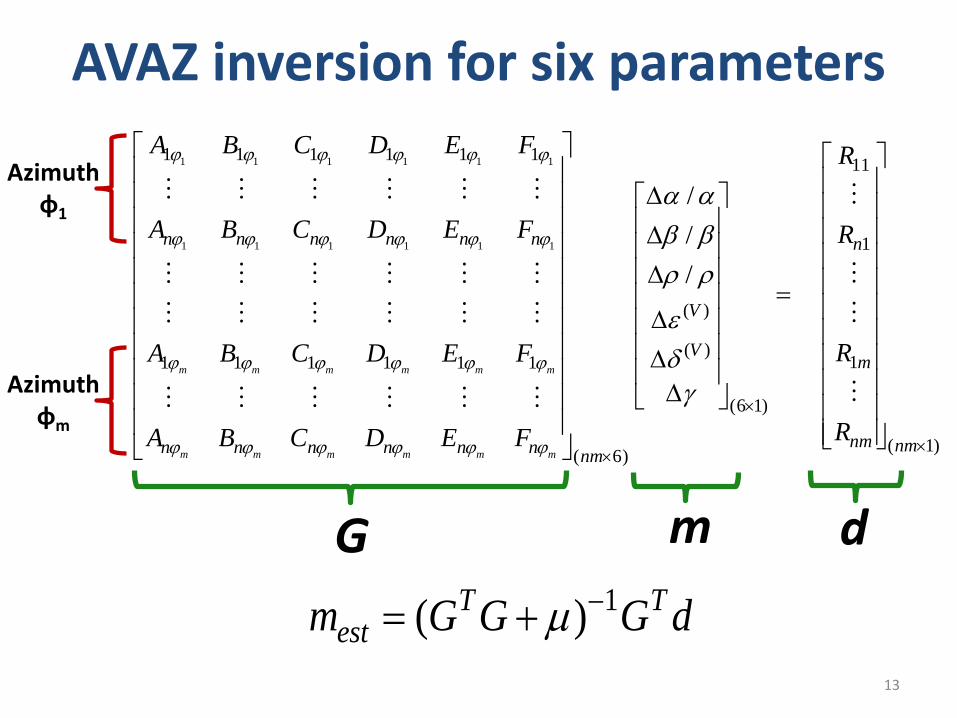
AVAZ inversion for six parameters 1 1 1 1 1 1

1 1 1 1 1 1

1 1 1 1 1 1

( )

( )1 1 1 1 1 1

(6 1)

( 6)

///

m m m m m m

m m m m m m

n n n n n n

V

V

n n n n n n nm

A B C D E F

A B C D E F

A B C D E F

A B C D E F

ϕ ϕ ϕ ϕ ϕ ϕ

ϕ ϕ ϕ ϕ ϕ ϕ

ϕ ϕ ϕ ϕ ϕ ϕ

ϕ ϕ ϕ ϕ ϕ ϕ

α αβ βρ ρ

εδγ ×

×

∆ ∆ ∆

= ∆

∆ ∆

11

1

1

( 1)

n

m

nm nm

R

R

R

R ×

1( )T Testm G G G dµ −= +

Azimuth φ1

Azimuth φm

G m d

13

14

AVAZ inversion for six parameters (errors WRT traveltime inversion results)

150

50

-50

% e

rror

Δ /β β Δ /ρ ρ ( )Vε ( )Vδ γΔα/α

Max incident angle = 37°

15

AVAZ inversion for six parameters (errors WRT traveltime inversion results))

150

50

-50

% e

rror

150

50

-50

% e

rror

Δ /β β Δ /ρ ρ ( )Vε ( )Vδ γΔα/α

Max incident angle = 37° Max incident angle = 41°

Δα/α Δ /β β Δ /ρ ρ ( )Vε ( )Vδ γ

Max incident angle = 45° Max incident angle = 49°

1. Determine ( ∆α/α, ∆β/β, ∆ρ/ρ ) from logs, or from conventional AVA inversion of isotropic plane direction. 2. Invert for ( ∆ε(V), ∆δ(V), ∆γ ) using Rüger’s equation constrained by results from step 1.

16

AVAZ inversion for three-parameters (anisotropy parameters)

17

20

-20

-40

% e

rror

0

Δαα

( )Vε ( )Vδ γ ( )Vε ( )Vδ γ

AVAZ inversion 6-parameter vs. 3-parameter

Max incident angle = 41⁰

Favourable results compared to those obtained previously by traveltime inversion

Directly related to fracture intensity

Δββ

Δρρ

Fracture symmetry axis not known

( )

2 22 2

2 2 2

24 2 2 2 2

2

2 2 2

0

02

0

0 0

1 4 1 4( , ) sin + 1 sin22cos

1 4 cos ( )sin tan cos ( )sin2

1 cos ( )sin cos ( )sin ( )2

HTIPPR α β β β ρθ φ θ θ

α β ρθ α α

βφ θ θ ε φ θ γα

φ θ φ φ

φ φ

φ φ φ

∆ ∆ ∆≅ − − +

− ∆ + − ∆ +

− + − −( )2 2sin tan

θ θ δ∆

: fracture system : acquisition coordinate φ : source-receiver azimuth φ0 : fracture symmetry direction

X1

X2

X3

φ0 φ

18

HTI: PP reflection coefficient Small incident angle ( θ < 35⁰ )

2 22 2

2 2 2

22 2( )

02

20

21 2

1 4 1 4( , ) sin + 1 sin22cos

4 1 cos ( )sin 2

( , ) cos ( ) sin

HTIPP

HTIP

V

P

R

R I G G

γ δ

α β β β ρθ φ θ θα β ρθ α α

β φ θα

θ ϕ φ θ

φ

φ

∆ ∆ ∆≅ − − +

+ + −

≅ + + −

∆ ∆

Isotropic gradient

Anisotropic gradient

gradient non-linear with respect to (G1,G2, φ0)

2

2)

2(4 1

2VG γβ

αδ∆+∆=

19

AVO intercept Q = AVO gradient

Estimate fracture orientation ( Grechka and Tsvankin (1998); Jenner (2002) )

21 2

2 21 2

0

10 0

Q cos ( )

( ) cos ( ) sin ( )

G G

G G G

ϕ

ϕ

ϕ

ϕ ϕϕ

= + −

= + − + −

20

x1

x2

0φ. φ

2 21 2 1 1 2Q ( )G G y G y= + +

Coordinate system aligned with fractures

1 0

2 0

cos( )sin( )

y ry r

φ φφ φ

= − = −

1

2

cossin

x rx r

φφ

= =

[ ]

2 211 1 12 1 2 22 2

11 12 11 2

12 22 2

Q = 2

W x W x x W xW W x

x xW W x

+ +

=

Acquisition coordinate system

2 211 12 22 cos 2 cos sin sinW W Wφ φ φ φ= + +

012

11 22

2tan( )2 WW W

φ =−

2 21 1 2 2 1,2 Q ( : igenvalues)y y eλ λ λ= +

2 2(1) 1 11 22 11 22 120

12

2 2( 2) 1 11 22 11 22 120

12

( ) 4tan

2

( ) 4tan

2

W W W W WW

W W W W WW

φ

φ

−

−

− + − + = − − − + =

(2) (1)0 0 2

πφ φ= +

21

Accurate prediction of fracture orientation requires extra geological info, or azimuthal NMO velocity.

Estimate fracture orientation ( Grechka and Tsvankin (1998); Jenner (2002) )

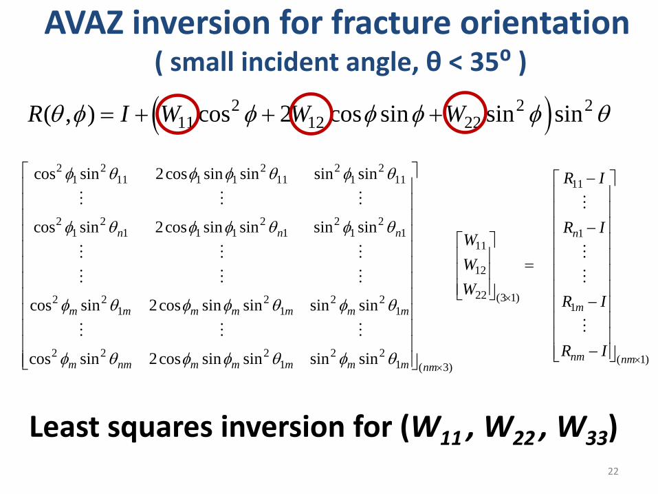
AVAZ inversion for fracture orientation ( small incident angle, θ < 35⁰ )

2 2 2 2 21 11 1 1 11 1 11

2 2 2 2 21 1 1 1 1 1 1

2 2 2 2 21 1 1

2 2 2 2 21 1

cos sin 2cos sin sin sin sin

cos sin 2cos sin sin sin sin

cos sin 2cos sin sin sin sin

cos sin 2cos sin sin sin sin

n n n

m m m m m m m

m nm m m m m m

φ θ φ φ θ φ θ

φ θ φ φ θ φ θ

φ θ φ φ θ φ θ

φ θ φ φ θ φ θ

11

111

12

22 (3 1)1

( 1)( 3)

n

m

nm nmnm

R I

R IWWW

R I

R I

×

××

− − = − −

( )2 2 211 12 22( , ) cos 2 cos sin sin sinR I W W Wθ φ φ φ φ φ θ= + + +

22

Least squares inversion for (W11 , W22 , W33)

Test on physical model data, AVAZ inversion φ0 = 30⁰

X1 φ0

True φ0 30⁰

Estimate φ0 28.5⁰ and 118.5⁰

φ0: fracture symmetry axis azimuth

23

Testing different fracture orientations

φ0: fracture symmetry axis azimuth

24

True φ0 0⁰ 10⁰ 20⁰ 40⁰ 60⁰ 80⁰ 90⁰

Estimate φ0 -1.5⁰

88.5⁰

8.5⁰

98.5⁰

18.5⁰

108.5⁰

38.5⁰

128.5⁰

58.5⁰

148.5⁰

78.5⁰

168.5⁰

88.5⁰

178.5⁰

Conclusions • Rüger equation for HTI, PP reflection coefficient, can be

used in an inversion for anisotropy parameters, but fracture orientation must be known.

• Knowing the fracture orientation, fracture intensity can be estimated from AVAZ inversion of large-offset data .

• Fracture orientation can be determined from AVAZ inversion of small incident angle data, but with 90⁰ ambiguity.

• Implementation on physical model data gives results consistent with these theories.

25

Acknowledgments

• CREWES sponsors • Dr. Joe Wong • Xinxiang Li • Dr. P.F. Daley • Dr. Kris Innanen • David Henley • Marcus Wilson • Mahdi Al-Mutlaq

26