automated profiling of individual cell-cell interactions from high

Bioimage informatics

Automated profiling of individual cell–cell

interactions from high-throughput time-lapse

imaging microscopy in nanowell grids (TIMING)

Amine Merouane1, Nicolas Rey-Villamizar1, Yanbin Lu1, Ivan Liadi2,

Gabrielle Romain2, Jennifer Lu2, Harjeet Singh3, Laurence J.N. Cooper3,

Navin Varadarajan2,* and Badrinath Roysam1,*

1Department of Electrical and Computer Engineering and 2Department of Chemical and Biomolecular Engineering,

University of Houston, Houston, TX, USA and 3Division of Pediatrics, The University of Texas MD Anderson Cancer

Center, Houston, TX, USA

*To whom correspondence should be addressed.

Associate Editor: Robert Murphy

Received on September 15, 2014; revised on June 1, 2015; accepted on June 4, 2015

Abstract

Motivation: There is a need for effective automated methods for profiling dynamic cell–cell inter-

actions with single-cell resolution from high-throughput time-lapse imaging data, especially, the

interactions between immune effector cells and tumor cells in adoptive immunotherapy.

Results: Fluorescently labeled human T cells, natural killer cells (NK), and various target cells

(NALM6, K562, EL4) were co-incubated on polydimethylsiloxane arrays of sub-nanoliter wells

(nanowells), and imaged using multi-channel time-lapse microscopy. The proposed cell segmenta-

tion and tracking algorithms account for cell variability and exploit the nanowell confinement prop-

erty to increase the yield of correctly analyzed nanowells from 45% (existing algorithms) to 98% for

wells containing one effector and a single target, enabling automated quantification of cell loca-

tions, morphologies, movements, interactions, and deaths without the need for manual proofread-

ing. Automated analysis of recordings from 12 different experiments demonstrated automated

nanowell delineation accuracy >99%, automated cell segmentation accuracy >95%, and auto-

mated cell tracking accuracy of 90%, with default parameters, despite variations in illumination,

staining, imaging noise, cell morphology, and cell clustering. An example analysis revealed that

NK cells efficiently discriminate between live and dead targets by altering the duration of conjuga-

tion. The data also demonstrated that cytotoxic cells display higher motility than non-killers, both

before and during contact.

Contact: [email protected] or [email protected]

Supplementary information: Supplementary data are available at Bioinformatics online.

1 Introduction

Dynamic cell behaviors, especially cell–cell interactions, are of vital

interest in immunology (Romain et al., 2014; Vanherberghen et al.,

2013; Varadarajan et al., 2012; Zaretsky et al., 2012), cancer biol-

ogy (Wang et al., 2012; Yin et al., 2008; Zheng et al., 2012) and

stem cell engineering (Ma et al., 2013; Zhao et al., 2011).

Automated time-lapse microscopy of live cells in vitro is a well-es-

tablished method for spatiotemporal recording of cells and biomol-

ecules, and tracking multi-cellular interactions. Unfortunately, most

conventional methods assess limited numbers (10–100) of manually

VC The Author 2015. Published by Oxford University Press. All rights reserved. For Permissions, please e-mail: [email protected] 3189

Bioinformatics, 31(19), 2015, 3189–3197

doi: 10.1093/bioinformatics/btv355

Advance Access Publication Date: 9 June 2015

Original Paper

Downloaded from https://academic.oup.com/bioinformatics/article-abstract/31/19/3189/212047by gueston 13 February 2018

http://bioinformatics.oxfordjournals.org/lookup/suppl/doi:10.1093/bioinformatics/btv355/-/DC1

http://www.oxfordjournals.org/

sampled ‘representative’ cell pairs, leading to subjective bias and

therefore lack the ability to quantify the behaviors of statistically

under-represented cells reliably. This is significant since many bio-

logically significant cellular subpopulations like tumor stem cells,

multi-killer immune cells and biotechnologically relevant protein se-

creting cells, are rare. There is a need for methods to sample cell–cell

interaction events on a larger scale to investigate such cellular phe-

nomena. Recent advances have enabled the fabrication of large

arrays of sub-nanoliter wells (nanowells) cast onto transparent bio-

compatible polydimethylsiloxane substrates (Forslund et al. 2012;

Ostuni et al., 2001; Rettig and Folch, 2005; Whitesides and Stroock,

2001). Small groups of living cells from clinical samples, and labora-

tory-engineered cells can be confined to nanowells, and imaged over

extended durations by multi-channel time-lapse microscopy, allow-

ing thousands of controlled cellular events to be recorded as an array

of multi-channel movies (Liadi et al., 2013; Varadarajan et al.,

2012). We refer to this method as Time-lapse Imaging Microscopy

In Nanowell Grids (TIMING). The spatial confinement can enable a

rich sampling of localized cellular phenomena, including cell move-

ments, cellular alterations, and cell–cell interaction patterns, along

with the relevant intra-cellular event markers (Pham et al., 2013).

TIMING is thus ideally suited for tracking cell migration and inter-

actions at short distances but if cell migratory patterns over larger

distances are of interest, arrays with larger wells can be fabricated.

Similarly, if unconfined migratory behavior of cells is desired, other

methods have been described (Sackmann et al., 2014). The promise

and challenge of nanowell arrays, is high throughput, eliminating

the need for user selection of events of interest, and the ability to re-

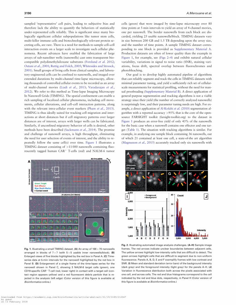
peatedly follow the same cell(s) over time. Figure 1 illustrates a

TIMING dataset consisting of >11 000 nanowells containing fluo-

rescently tagged human CARþ T-cells (red) and NALM-6 tumor

cells (green) that were imaged by time-lapse microscopy over 80

time points at 5-min intervals to yield an array of 4-channel movies,

one per nanowell. The border nanowells from each block are dis-

carded, yielding 25 usable nanowells/block. TIMING datasets vary

in size between 200 GB and 1.5 TB depending upon the array size,

and the number of time points. A sample TIMING dataset corres-

ponding to one block is provided as Supplementary Material A.

Production datasets are often of lower quality than the example in

Figure 1, for example, see (Figs 2–4) and exhibit natural cellular

variability, variations in signal to noise ratio (SNR), staining vari-

ations, focus drift, spectral overlap between fluorochromes and

photobleaching.

Our goal is to develop highly automated pipeline of algorithms

that can reliably segment and track the cells in TIMING datasets with

minimal parameter tuning, and yield a sufficiently rich set of cellular-

scale measurements for statistical profiling, without the need for man-

ual proofreading (Supplementary Material B). A direct application of

general-purpose segmentation and tracking algorithms is not a viable

strategy since their yield (the number of correctly analyzed nanowells)

is surprisingly low, and their parameter tuning needs are high. For ex-

ample, a direct application of Al-Kofahi et al. (2010) segmentation al-

gorithm with a reported accuracy >95% that is the core of the open-

source FARSIGHT toolkit (farsight-toolkit.org) to the dataset in

Figure 1 produces an error-free yield of only 43% of the nanowells

for the basic case when a nanowell contains one effector and one tar-

get (Table 1). The situation with tracking algorithms is similar. For

example, in analyzing one sample block containing 36 nanowells, out

of which 21 contained at least one cell, a state-of-the art algorithm

(Magnusson et al., 2015) accurately tracked only six nanowells with

Fig. 1. Illustrating a small TIMING dataset. (A) An array of 168� 70 nanowells

arranged in blocks of 7�7 (with 5�5 usable inner nanowells/block). (B)

Enlarged views of five blocks highlighted by the red box in Panel A. (C) Time-

series data at 5-min intervals for the nanowell highlighted by the red box in

Panel B. (D) Enlargement of a single frame of the time-lapse series for the

nanowell shown in Panel C, showing 3 NALM-6 target cells (green), one

CD19-specific CARþ T-cell (red, lower right) in contact with a target cell (con-

tact region appears yellow) and a red fluorescent debris particle that is re-

jected in the analysis (left edge) (Color version of this figure is available at

Bioinformatics online.)

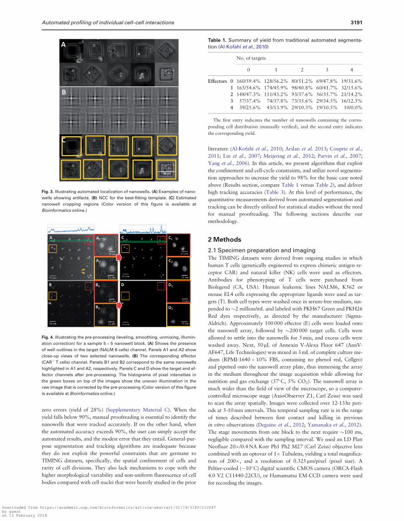
Fig. 2. Illustrating automated image analysis challenges. (A–H) Sample image

frames. The red arrows indicate unclear boundaries between adjacent cells.

The yellow arrows highlight low-intensity cells that are difficult to detect. The

green arrows highlight cells that are difficult to segment due to non-uniform

fluorescence. Panels A, B, D, E and F exemplify frames with low contrast and

SNR. (I) Mean and standard deviation (error bars) of the background intensity

(dark gray) and the foreground intensity (light gray) for the panels A–H. (J)

Variation in fluorescence distribution both across the pixels associated with

one cell, and across cells. The red and blue histograms correspond to the cell

indicated by the red and blue dots, respectively, in Panel H (Color version of

this figure is available at Bioinformatics online.)

3190 A.Merouane et al.




zero errors (yield of 28%) (Supplementary Material C). When the

yield falls below 90%, manual proofreading is essential to identify the

nanowells that were tracked accurately. If on the other hand, when

the automated accuracy exceeds 90%, the user can simply accept the

automated results, and the modest error that they entail. General-pur-

pose segmentation and tracking algorithms are inadequate because

they do not exploit the powerful constraints that are germane to

TIMING datasets, specifically, the spatial confinement of cells and

rarity of cell divisions. They also lack mechanisms to cope with the

higher morphological variability and non-uniform fluorescence of cell

bodies compared with cell nuclei that were heavily studied in the prior

literature (Al-Kofahi et al., 2010; Arslan et al. 2013; Couprie et al.,

2011; Lin et al., 2007; Meijering et al., 2012; Parvin et al., 2007;

Yang et al., 2006). In this article, we present algorithms that exploit

the confinement and cell-cycle constraints, and utilize novel segmenta-

tion approaches to increase the yield to 98% for the basic case noted

above (Results section, compare Table 1 versus Table 2), and deliver

high tracking accuracies (Table 3). At this level of performance, the

quantitative measurements derived from automated segmentation and

tracking can be directly utilized for statistical studies without the need

for manual proofreading. The following sections describe our

methodology.

2 Methods

2.1 Specimen preparation and imagingThe TIMING datasets were derived from ongoing studies in which

human T cells (genetically engineered to express chimeric antigen re-

ceptor CAR) and natural killer (NK) cells were used as effectors.

Antibodies for phenotyping of T cells were purchased from

Biolegend (CA, USA). Human leukemic lines NALM6, K562 or

mouse EL4 cells expressing the appropriate ligands were used as tar-

gets (T). Both cell types were washed once in serum-free medium, sus-

pended to �2 million/mL and labeled with PKH67 Green and PKH26

Red dyes respectively, as directed by the manufacturer (Sigma-

Aldrich). Approximately 100 000 effector (E) cells were loaded onto

the nanowell array, followed by �200 000 target cells. Cells were

allowed to settle into the nanowells for 5 min, and excess cells were

washed away. Next, 50mL of Annexin V-Alexa Fluor 647 (AnnV-

AF647, Life Technologies) was mixed in 3 mL of complete culture me-

dium (RPMI-1640þ10% FBS, containing no phenol red, Cellgro)

and pipetted onto the nanowell array plate, thus immersing the array

in the medium throughout the image acquisition while allowing for

nutrition and gas exchange (37�C, 5% CO2). The nanowell array is

much wider than the field of view of the microscope, so a computer-

controlled microscope stage (AxioObserver Z1, Carl Zeiss) was used

to scan the array spatially. Images were collected over 12-13hr peri-

ods at 5-10 min intervals. This temporal sampling rate is in the range

of times described between first contact and killing in previous

in vitro observations (Deguine et al., 2012; Yamanaka et al., 2012).

The stage movements from one block to the next require �100 ms,

negligible compared with the sampling interval. We used an LD Plan

Neofluar 20�/0.4NA Korr Ph1 Ph2 M27 (Carl Zeiss) objective lens

combined with an optovar of 1� Tubulens, yielding a total magnifica-

tion of 200�, and a resolution of 0.325mm/pixel (pixel size). A

Peltier-cooled (�10�C) digital scientific CMOS camera (ORCA-Flash

4.0 V2 C11440-22CU), or Hamamatsu EM-CCD camera were used

for recording the images.

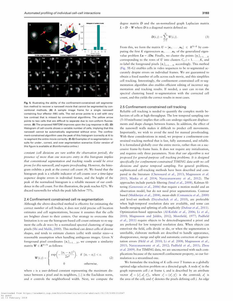
Fig. 3. Illustrating automated localization of nanowells. (A) Examples of nano-

wells showing artifacts. (B) NCC for the best-fitting template. (C) Estimated

nanowell cropping regions (Color version of this figure is available at

Bioinformatics online.)

Fig. 4. Illustrating the pre-processing (leveling, smoothing, unmixing, illumin-

ation correction) for a sample 5�5 nanowell block. (A) Shows the presence

of well outlines in the target (NALM-6 cells) channel. Panels A1 and A2 show

close-up views of two selected nanowells. (B) The corresponding effector

(CARþ T cells) channel. Panels B1 and B2 correspond to the same nanowells

highlighted in A1 and A2, respectively. Panels C and D show the target and ef-

fector channels after pre-processing. The histograms of pixel intensities in

the green boxes on top of the images show the uneven illumination in the

raw image that is corrected by the pre-processing (Color version of this figure

is available at Bioinformatics online.)

Table 1. Summary of yield from traditional automated segmenta-

tion (Al-Kofahi et al., 2010)

No. of targets

0 1 2 3 4

Effectors 0 160/59.4% 128/56.2% 80/51.2% 69/47.8% 19/31.6%

1 165/54.6% 174/45.9% 98/40.8% 60/41.7% 32/15.6%

2 148/47.3% 111/43.2% 93/37.6% 56/35.7% 21/14.2%

3 57/37.4% 74/37.8% 73/35.6% 29/34.5% 16/12.5%

4 39/25.6% 43/13.9% 29/10.3% 19/10.5% 10/0.0%

The first entry indicates the number of nanowells containing the corres-

ponding cell distribution (manually verified), and the second entry indicates

the corresponding yield.

Automated profiling of individual cell–cell interactions 3191



2.2 Automatic nanowell localizationAutomatic localization of nanowells is necessary for delineating the

cell confinement regions, correcting for stage re-positioning errors,

and breaking up the overall TIMING dataset into a large number of

motion-corrected video sequences, one per nanowell. This operation

must be reliable since a single well-detection error can render the

nanowell unusable for analysis, reducing the experimental yield. It

must be robust to focus drift (accounting for shrinkage/swelling/ir-

regularity of the polymer substrate), wells with compromised geom-

etry, illumination variations, ringing artifacts and debris or air

bubbles that may move, and abruptly appear/disappear from the

camera view over time (Fig. 3A).

Content-independent image registration methods like SIFT

matching (Li et al., 2010) were neither sufficiently reliable nor prac-

tical for TIMING data. They required multiple parameter adjust-

ments, and failed in the presence of artifacts. Therefore, we adopted

a normalized cross-correlation (NCC) based template fitting method

that is robust to illumination variations and artifacts (Yoo and Han,

2009). We exploited the fact that the geometry of nanowells is

known from the fabrication process, and they are always visible in

the phase-contrast channel. Note in Figure 1B that some of the

nanowells are intentionally rotated by 45� for implementing a cod-

ing strategy designed to uniquely locate individual wells in an array.

Therefore, we select two empty wells (regular and rotated by 45�)

from the dataset being analyzed and use them as templates that are

fitted to the image data. The NCC responses are in the range of (�1,

þ1), with �1 indicating a poor match, and þ1 a perfect match. To

speed up NCC, we used a Fourier implementation, and performed

the normalization in the spatial domain. Figure 3B shows the NCC

responses of the example wells in Figure 3A to the best-fitting (of

the two) templates in Figure 3A. We used the local maximum clus-

tering algorithm (Wu et al., 2004) on the best-fitting NCC response

to detect well centers, and used the known spacing between nano-

wells to filter out invalid responses, yielding a robust localization of

wells with >99% accuracy (Section 3). To cope with artifacts, we

discard the nanowell videos whose maximum NCC response falls

below a predefined threshold (typ. 0.75). The resulting rigid spatial

transformation estimates (Fig. 3C) are used to generate cropped mo-

tion-corrected nanowell video recordings.

2.3 Image pre-processingEach image frame of every video sequence is leveled to correct illu-

mination variations by subtracting the local background estimated

at each pixel using a Gaussian kernel with r¼15 (Fig. 4). Next, we

correct for spectral overlap between the emission spectra of the

PKH67 and PKH26 dyes used to label the effector and target cells.

The columns of the mixing matrix are estimated offline using princi-

pal component analysis for a 7�7 block of nanowell videos, and

then re-used across the rest of the array. The unmixing was per-

formed by the linear inverse method (Keshava and Mustard, 2002).

Finally, we smooth the images using a median filter with radius

rm¼3 while preserving cell boundaries. As noted by other authors,

such pre-processing is essential for reducing high-throughput cell

segmentation errors (Singh et al., 2014).

Even after pre-processing, cells exhibit variability in shape and intra-

cellular fluorescence (Fig 5A), and this is a challenge for cell detection and

separation of touching/overlapping cell bodies. The widely used multi-

scale Laplacian of Gaussian (LoG) map (Al-Kofahi et al., 2010) misses

the dim cell indicated by the red arrow, and is unable to separate the pair

of cells indicated by the yellow arrow that exhibit non-round shapes and

non-uniform intensities (Fig. 5C). Gradient-weighted watershed algo-

rithms (e.g. Lin et al., 2007) have difficulty separating cells with weak

edges. In order to overcome these limitations, we propose a normalized

multi-threshold distance map (NMTDM) (Fig. 5C) that is designed to de-

tect cell bodies, and it works by averaging distance maps corresponding

to multiple thresholds, as follows. First, the normalized pixel intensity dis-

tributions p (i) of our pre-processed images are modeled by a mixture of

3 Gaussian distributions pðiÞ ¼XK

k¼1wkgði j lk; rkÞ, with parameters

ðlk;rkÞ and weights wk, k ¼ 1; 2; 3 that capture the dim background,

intermediate foreground, and hyper-fluorescent foreground pixels, re-

spectively. We use the k-means algorithm with deterministic seeding for

estimating the mixture weights since it is fast, requires few initialization

parameters, converges reliably, and produces comparable results to ex-

pensive expectation maximization algorithms, making it ideal for our

high-throughput analysis. Clusters 2 and 3 together capture the image

foreground. This foreground is divided into a set of connected compo-

nents denoted Rh; h ¼ 1; . . . ;H. Next, let Lmin and Lmax denote the

minimum and maximum pixel intensity values for this foreground.

We define a series of M threshold levels (typ. 20) denoted l

between Lmin and Lmax separated by d ¼ ðLmax � LminÞ=M, so

l ¼ Lmin; Lmin þ d; Lmin þ 2d; . . . ; Lmax. Each of these thresholds is

used to generate a corresponding binary mask denoted Blðx; yÞ and a

corresponding Euclidean distance map Dlðx; yÞ. We then normalize

the Euclidean distance maps for each connected component by the cor-

responding maximum value within each connected component Rh, to

ensure that the distance maps at different levels contribute equally to

the final response. With this, the NMTDM for each connected compo-

nent Rh can be written as the following pixel-level average of normal-

ized distances across the thresholding levels l:

NMTDM�ðx; yÞ 2 Rh

�¼ 1

M�X

l

Dlððx; yÞ 2 RhÞmaxðx;yÞ

Dlððx; yÞ 2 RhÞ(1)

Note that the NMTDM computation is only performed for the fore-

ground pixels, and can be carried out efficiently in parallel for differ-

ent connected components. This map exhibits much clearer peaks

compared with the multi-scale LoG (Fig. 5B versus C), and allows

reliable cell detection.

Individual cells are detected using local maxima clustering over the

NMTDM (Wu et al., 2004). This step requires only two parameter

settings: the number of levels M, and the clustering radius r for select-

ing the peaks. Using this, we estimate the number of cells independ-

ently for each frame, and compute a histogram over the time series

(Fig. 5D). Knowing that the number of cells in a nanowell stays

Table 2. Summary of error-free nanowell yield using the confine-

ment constrained cell detection method

No. of Targets

0 1 2 3 4

Effectors 0 160/99.4% 128/98.4% 80/97.5% 69/92.8% 19/89.5%

1 165/98.7% 174/98.3% 98/97.9% 60/91.7% 32/78.1%

2 148/97.9% 111/97.3% 93/96.8% 56/91.1% 21/80.9%

3 57/94.7% 74/94.6% 73/91.8% 29/89.7% 16/81.2%

4 39/87.1% 43/88.4% 29/86.2% 19/84.2% 10/80.0%

Table 3. Frequency of cell segmentation and tracking errors

Number of cells 2 targets 3 targets 4 targets

Under-segmentation 1.2% 1.4% 0.1%

Over-segmentation 1.3% 0.6% 4.2%

Incorrect-correspondence 0.9% 0.8% 3.6%

Total cells validated 816 636 168



constant (cell divisions are rare within the observation period), the

presence of more than one non-zero entry in this histogram implies

that conventional segmentation and tracking results would be error

prone for this nanowell, and require proofreading. However, the histo-

gram exhibits a peak at the correct cell count (4). We found that the

histogram peak is a reliable indicator of cell counts over a time-lapse

sequence despite errors in individual frames, and the height of the

peak of the normalized histogram is a reliable measure of our confi-

dence in the cell count. For this illustration, the peak reaches 82%. We

discard nanowells for which the peak falls below 75%.

2.4 Confinement constrained cell re-segmentationAlthough the above-described method is effective for estimating the

correct number of cell bodies, it does not yield precise cell location

estimates and cell segmentations, because it assumes that the cells

are brighter closer to their centers. Our strategy to overcome this

limitation is to use the histogram-based cell count estimate to re-seg-

ment the cells de novo by a normalized spectral clustering of image

pixels (Shi and Malik, 2000). This method can detect cells of diverse

shapes, and tends to estimate clusters (cells) with similar sizes—a

reasonable assumption when handling ambiguous images. Given N

foreground pixel coordinates fxigi¼1; ... ;N, we compute a similarity

matrix W 2 RN�N as follows:

Wði; jÞ ¼exp � jjxi � xjjj2

2r2

� �; if jjxi � xjjj < e;

0 otherwise;

8>><>>:

(2)

where e is a user-defined constant representing the maximum dis-

tance between a pixel and its neighbors, jj:jj is the Euclidean norm,

and r controls the neighborhood width. Next, we compute the

degree matrix D and the un-normalized graph Laplacian matrix

L¼D�W where D is a diagonal matrix defined as:

Dði; jÞ ¼XNj¼1

Wði; jÞ: (3)

From this, we form the matrix U ¼ ½u1; . . . ;uK� 2 RN�K by com-

puting the first K eigenvectors u1; . . . ;uK of the generalized eigen-

value problem Lu ¼ kDu. Finally, we cluster the points fyigi¼1; ... ;N

corresponding to the rows of U into clusters Ci; i ¼ 1; . . . ;K, and

re-label the foreground pixels fxigi¼1; ... ;N accordingly. This method

(Fig. 5E–G) enables cells in video sequences to be re-segmented ac-

curately despite errors on individual frames. We are guaranteed to

obtain a fixed number of cells across each movie, and this simplifies

cell tracking. Interestingly, the confinement constrained cell re-seg-

mentation algorithm also enables efficient editing of incorrect seg-

mentation and tracking results. If needed, a user can re-run the

spectral clustering based re-segmentation with the corrected cell

count, and this yields the correct results in most cases.

2.5 Confinement-constrained cell trackingReliable cell tracking is needed to quantify the complex motile be-

haviors of cells at high throughput. The low temporal sampling rate

(5–10 min/frame) implies that cells can undergo significant displace-

ments and shape changes between frames. In addition, the effect of

the nanowell walls makes it difficult to predict cell movements.

Importantly, we wish to avoid the need for manual proofreading.

With these considerations in mind, we propose a confinement-con-

strained tracking method that is fast, fully automated, and reliable.

It is formulated globally over the entire movie, rather than on a suc-

cessive frame-by-frame basis. It does not require any initialization,

and requires only three parameters. Note that our algorithm is not

proposed for general-purpose cell tracking problems. It is designed

specifically for confinement-constrained TIMING data with no cell

divisions and sparse temporal sampling. For general problems,

sophisticated cell-tracking methods have been described and com-

pared in the literature (Chenouard et al., 2013; Magnusson et al.

2015; Maska et al. 2014; Narayanaswamy et al., 2012). The

approaches include particle filtering (Smal et al., 2008), Kalman fil-

tering (Genovesio et al., 2006) that require a motion model and an

observation model, but do not need prior segmentations. Contour

based (Mukherjee et al., 2004), mean-shift (Comaniciu et al., 2000)

and level-set methods (Dzyubachyk et al., 2010), are preferable

when high-temporal resolution data are available, and some can

handle merging and splitting of cells implicitly (Dufour et al., 2011).

Optimization-based approaches (Al-Kofahi et al., 2006; Li et al.,

2010; Magnusson and Jalden, 2012; Morefield, 1977; Padfield

et al., 2011) require objects to be detected/segmented a priori and

are preferred for low temporal resolution data. When objects can

enter/exit the field, cells divide or die, or when the segmentation is

unreliable, elaborate methods are described to handle appearance,

disappearance, merge and split and automatic correction of segmen-

tation errors (Held et al. 2010; Li et al. 2008; Magnusson et al.,

2015; Narayanaswamy et al., 2012; Padfield et al., 2011; Zhou

et al. 2009). For TIMING data, we are unconcerned with such com-

plications because of the nanowell confinement property, so our for-

mulation is a streamlined one.

We formulate the tracking of K cells over T frames as a globally

optimal edge selection problem on a directed graph. A node ntj in the

graph represents cell j at frame t, and is described by an attribute

vector dtj ¼ fct

j ; atj ; r

tjg, where ct

j ¼ ðxtj ; y

tjÞ is the centroid; at

j is

the area of the cell; and rtj denotes the pixels defining cell j. An edge

Fig. 5. Illustrating the ability of the confinement-constrained cell segmenta-

tion method to recover a nanowell movie that cannot be segmented by con-

ventional methods. (A) A sample image frame for a single nanowell

containing four effector (NK) cells. The red arrow points to a cell with very

low contrast that is missed by conventional algorithms. The yellow arrow

points to two cells that are difficult to separate due to non-uniform fluores-

cence. (B) The proposed NMTDM improves upon the Log response in (C). (D)

Histogram of cell counts shows a variable number of cells, implying that this

nanowell cannot be automatically segmented without error. The confine-

ment-constrained algorithm uses the peak of this histogram (correctly at 4) to

re-segment the entire movie correctly. (E–G) Examples of re-segmentation re-

sults for under-, correct, and over segmentation scenarios (Color version of

this figure is available at Bioinformatics online.)



eti;j ¼ fnt�1

i ; ntjg associates cell i at frame t�1 to cell j at frame t, and

we compute an association cost utij that measures the dissimilarity

between cell regions i and j. An edge selection variable ctij 2 f0; 1g

indicates if a given edge is selected in the final solution.

Using integer programming, we seek the solution c 2 f0; 1gN, where

N ¼ ðT � 1Þ � K�K that minimizes the following sum of associ-

ation costs over each nanowell:

C ¼ arg minc2f0;1gN

XT

t¼2

XK

j¼2

XK

i¼1

uti;jc

ti;j;

s:t:

XK

i¼1ct

i;j�1 forj ¼ 1; . . . ;K;

t ¼ 2; . . . ;T:

XK

k¼1ctþ1

i;k �1 forj ¼ 1; . . . ;K;

t ¼ 2; . . . ;T � 1:

8>>>>>>><>>>>>>>:

(4)

The cell confinement constraint is implicit in this formulation.

The inequality constraints ensure that each node ntj is associated

with a maximum of one node in the previous frame, and the next

frame, respectively. In computing uti;j, we ignore shape and texture

features since cell morphologies and intensity profiles vary over

time. We compute a weighted sum of the Euclidean distance be-

tween cell centroids gðci; cjÞ, the area difference between cells

gðai; ajÞ ¼ jai � ajj, and the following set-theoretic distance between

the pixels ðri; rjÞ for the two cells:

gðri; rjÞ ¼1�

aoverlap

minðai; ajÞif voverlap > 0

min�

distðri; rjÞ�; otherwise;

8>><>>:

(5)

where aoverlap is the overlapping area, and min�

distðri; rjÞ�

is the

shortest distance between the cells’ pixels. The overall cost is written

as uij ¼ w1 � gðci; cjÞ þw2 � gðai; ajÞ þw3 � gðri; rjÞ, where the

weights w1, w2 and w3 can be adjusted if needed. We used the de-

fault values w1 ¼ 1, w2 ¼ 10, and w3 ¼ 100. One can increase w3

when high temporal resolution data and good segmentation results

are available. We solve the integer program in Equation (4) using

the branch-and-bound algorithm (Schrijver, 1998). Although the

theoretical worst-case running time can grow exponentially, this is

not a concern since we are processing small cohorts of cells in each

nanowell. Figure 6A illustrates the results of automated tracking for

a nanowell containing only effector cells, showing our ability to

cope with large inter-frame movements. Panels B–E depict sample

cell trajectories for effector and target cells with diverse motion pat-

terns. Additional examples are presented in Figure 8.

2.6 Detection and quantification of cell–cell contactsDetecting contacts between effectors and targets, and measuring the

contact parameters (e.g. onset time, duration, frequency, extent) is

needed for understanding how cell behaviors predict subsequent

events of interest, especially the killing of targets by effectors.

Approaches using the spatial proximity of cell segmentations (Chen

et al., 2009; Klauschen et al., 2009) can be unreliable for TIMING

data since they require much higher resolution imaging, and are sen-

sitive to segmentation errors. With this in mind, we define a soft cell

interaction measure CI for quantifying the interaction of a cell with

its surrounding cells, as follows. First, we compute the normalized

effector fluorescence signal IjNðx; yÞ in each nanowell j. Next, we de-

fine a series of ring-like compartments using a Euclidean distance

map Dðx; yÞ with respect to the segmented target cells as illustrated

in Figure 7. Pixels with distances between k and kþ 1 pixels form

compartments bk with inner radii k ¼ f1; 2; . . . ; ng, where n is the

maximum distance needed to cover the complete nanowell. We sum

the fluorescence intensities over each compartment, and normalize

them by their radii k that are proportional to the compartment

areas. With this, the cell interaction measure CIðtÞ is the following

weighted intensity summation:

CIðtÞ ¼Xn

k¼1

1

k

Xðx;yÞ2bk

IjNðx; yÞ

� �: (6)

Figure 7 shows how CI (t) captures contacts between NK cells and

K562 cells in a graded manner over an image sequence. This measure

can be thresholded to detect contact events with a desired sensitivity.

The threshold is set and verified manually by an immunologist based

on visual verification of at least 30 nanowells for each TIMING data-

set, starting with a default value (typ. 0.01). We consider this visual

verification to be valuable due diligence. A full manual annotation of

the contacts by five independent observers over 156 nanowell videos

showed a 90.4% concordance with the default threshold. In order to

definitely assign contact, it is defined to occur when the threshold cri-

terion is met for two successive frames. The CIðtÞ measure is defined

above for a single cell and its neighbors. It can be extended to handle

multiple cells by using the segmentation masks.

2.7 Feature computationFor each cell, the automated segmentation and tracking operations

produce multiple time series of primary features including cell loca-

tion ðx; yÞ, area aðtÞ, instantaneous speed vðtÞ, cell shape as meas-

ured by the eccentricity of the best-fitting ellipse eðtÞ, and the

contact measure CIðtÞ. In addition, target cell death events (apop-

tosis) are detected using Annexin V whose summed fluorescence in-

tensity idðtÞ, is measured as another primary feature. Next, we

compute cellular features at the scale of each nanowell, specifically,

the number of effector cells ne, target cells nt, dead effectors ned,

contacted targets ntc, and killed targets ntk. These measurements can

be used to profile the nanowells.

The primary cellular features capture essential aspects of the cel-

lular activities within each nanowell, but they have two disadvan-

tages. First, they have a variable dimensionality, since the number of

time points varies across TIMING experiments. Second, a long

Fig. 6. Illustrating confinement-constrained cell tracking. (A) Sample tracking

of NK cells in a nanowell. The cell outlines are colored by cell identity. (B–E)

Color-coded sample cell movement paths illustrating the ability to track ef-

fector and target cells with diverse movement patterns (Color version of this

figure is available at Bioinformatics online.)



experiment can result in unnecessarily high-dimensional feature

data. With the intent of deriving meaningful lower-dimensional rep-

resentations of cellular events independent of the number of time

points, we derive a set of eight secondary features for each cell. For

each cell, we compute the average speed prior to first contact vfree,

average speed during the contact phase vcontact, average cell eccentri-

city prior to first contact efree, average eccentricity during the con-

tact phase econtact, time elapsed between first contact and death Dtd,

total contact duration between first contact and death Dtcd, time

duration before first contact Dtfree, the number of conjugations prior

to target cell death ncd.

3 Experimental results

The proposed method was evaluated on 12 TIMING experiments

involving combinations of target cells (NALM6, K562 and EL4) and

effector cells (NK cells or CARþT cells), to evaluate its ability to cope

with biological and imaging variability, different cell types, and vary-

ing experimental conditions. All the datasets were analyzed using the

parameter settings summarized in Table 4. Given the sheer volume of

the data, we start by presenting a visual summary of sample segmenta-

tion and tracking results in Figure 8. Overall, the algorithms and par-

ameter settings proved reliable for automated analysis. As a detailed

example, we present results of manually validating the segmentation

and tracking on a small dataset with 2000 nanowells containing

CARþT cells and NALM6 cells imaged over 70–80 time points. Of

these, 157 nanowells had more than four effectors or targets. These

larger cohorts are irrelevant for the current biological study of interest,

so they were omitted from further analysis. An additional 33 wells

(1.7%) were discarded because the confidence in cell counts (histo-

gram peak) was below 75%. Of the remaining 1803 nanowells, only

7 were not detected accurately due to air bubbles, so our overall nano-

well detection accuracy exceeds 99%.

3. 1 Improvement in yieldIn order to assess the fraction of wells with zero cell detection errors,

we manually validated the results over the 1803 remaining

nanowells using the proposed method and the (Al-Kofahi et al.,

2010) algorithm was used as a benchmark. The results are summar-

ized in Table 2. For the table entries with >90 wells, we manually

validated 40% of wells, and the full set of wells for the remaining

entries. Comparing the corresponding entries in Tables 1 and 2

show that the proposed method dramatically increased the number

of usable wells. The few errors were due to persistently dim fluores-

cent cells that were missed, or because a cell was persistently

occluded by another cell for >80% of the recording duration. For

perspective, yield rates <90% render the automated image analysis

results unusable, since the user has to manually analyze an excessive

number of nanowells. With a yield close to 98%, the user can simply

accept the automated results, and the modest error that they entail.

3.2 Cell segmentation and tracking performanceA total of 5061 cells were segmented and tracked in this dataset.

The automated segmentation and tracking results were overlaid on

the movies and presented to an immunologist, and the errors were

scored as: under-segmentation, over-segmentation and incorrect as-

sociation. Over-segmentation errors appear when a cell is identified

as two or more objects. Under-segmentation occurs when the same

label is assigned to multiple cells. Both of these errors can occur if

the cell count is incorrect. Incorrect correspondence occurs when the

tracking fails, usually due to segmentation errors. We consider a sin-

gle association error sufficient to render the tracking results for a

nanowell movie unusable. Despite this stringent requirement and

the high volume of data, the algorithm is extremely accurate

(Table 3). We next compared automatic segmentations of 30 ran-

domly selected target and effector cells against manual segmenta-

tions. The Jaccard similarity index for target cells was 0.86 6 0.12

(mean 6 SD.) and 0.78 6 0.17 for effector cells, indicating good seg-

mentation accuracy.

3.3 Data analysisWe analyzed a TIMING dataset containing 11 520 nanowells (320

blocks of 6�6 wells) in which we imaged the dynamics of killing of

K562 cells by in-vitro expanded NK cells for 8 h at 6-min intervals.

From the automatically extracted features, we selected only the

nanowells containing exactly one effector and one target cell, show-

ing a stable effector-target contact of at least 6 min (two successive

frames), and in the case of target death, contact by effector prior to

death. This resulted in a cohort of 552 nanowells that is ideal for

analyzing the dynamic behaviors of effectors, without the confounds

associated with multi-effector cooperation or serial killing.

Comparisons of the out-of-contact motility and the velocity during

tumor cell conjugation demonstrated that NK cells that participated

in killing displayed higher motility during both phases (Fig. 9A),

consistent with our recent report that demonstrated that motility

might be a biomarker for activated immune cells (Liadi et al., 2015).

Furthermore, for NK cells the change in speed and arrest upon target

cell ligation is well documented (Beuneu et al., 2009). Second, we

were also interested in quantifying differences in NK cell behavior in

interacting with live or dead cells. Of all the NK cells that partici-

pated in killing, only 18% re-conjugated to target cells subsequent

to apoptosis, and when they did, their duration of conjugation

18 6 14 min was significantly shorter than conjugations mediated by

the same NK cells to live tumor cells (52 6 72 min) (Fig. 9B). These

results suggest that NK cells largely avoided conjugating to dead tar-

get cells, and even when they did, made an early decision to termin-

ate the conjugation.

Fig. 7. Illustration of cell interaction analysis using the CI measure. (A) Spatial

regions used to compute CI for a target cell (K562 cell, green) and effector

(NK cell, red); (B) Contact event for which CI¼ 0.03; (C) Non-contact for which

CI¼ 0.007; (D) Sample frames over 5 h every 24 min. (E) The contact measure

CI variation over time for target cells (Color version of this figure is available

at Bioinformatics online.)



3.4 ImplementationFor a block with 36 wells and 60 cells, the processing time is 9–10 s/

block per time point on a Dell 910 PowerEdge server with 40 CPU

cores, 1 TB of RAM, and a RAID 5 storage system. The cell tracking

took 1.1 s/block; segmentation took 3.1 s/block; well detection took

1.5 s/block; and feature computation took 3.5 s/block. Various por-

tions of the software were implemented in Python and Cþþ, and

MATLAB (Supplementary Material D).

4 Conclusions

The combined TIMING system consisting of the nanowell arrays

and the proposed confinement-constrained image analysis methods

enables a far more comprehensive sampling of cellular events than is

possible manually. The proposed algorithms dramatically improved

the yield and accuracy of the automated analysis to a level at which

the automatically generated cellular measurements can be utilized

for biological studies directly, with little/no editing. Most segmenta-

tion and/or tracking errors (mostly due to persistently low

fluorescence (dim cells), or persistent cell occlusion over extended

durations) can be detected based on the histogram threshold

method, and the corresponding nanowells can either be ignored or

edited. Our pipeline is now in active use in several biological studies

being reported separately (e.g. Liadi et al., 2015; Romain et al.,

2014). It is scalable to multi-terabyte datasets, and does not require

elaborate initialization or careful parameter tuning. Supplementary

Material D includes the software for the computational pipeline that

enables routine, accurate, comprehensive, high-throughput, and

high-yield analysis of TIMING datasets on multi-core computers.

Acknowledgements

We thank Dr Vladimir Senyukov and Dr Dean Lee for providing cells, and Dr

Arvind Rao and Dr Joon Sang for informatics advice. This work was sup-

ported by the National Institutes of Health [R01CA174385]; the Cancer

Prevention Research Institute of Texas [RP130570]; Welch Foundation

[E1774] and the Melanoma Research Alliance Stewart-Rahr Young

Investigator Award (NV). We thank Dr Magnusson for sharing his code and

providing guidance.

Conflict of Interest: Dr. Cooper founded and owns InCellerate, Inc. He has

patents with Sangamo BioSciences with artificial nucleases. he consults with

Targazye, Inc (American Stem cells, Inc.), GE Healthcare, Ferring

Pharmaceuticals Inc., Bristol-Myers Squibb. None of these activities had any

influence on any part of this study.

References

Al-Kofahi,O. et al. (2006) Automated cell lineage construction: a rapid

method to analyze clonal development established with murine neural pro-

genitor cells. Cell Cycle, 5, 327–335.

Fig. 8. Visual summary of segmentation and tracking results involving vari-

ous target cells (NALM6, K562 and EL4) and effector cells (NK cell or CARþ T

cell) from 12 TIMING experiments, all run with identical parameter settings

(Table 4). The upper rows show sample frames. The middle rows show seg-

mentations. The bottom rows show the cell tracks (Color version of this figure

is available at Bioinformatics online.)

Table 4. List of parameter settings

Parameter Processing step Value (units)

Median filter size rm Pre-processing 3–5 (pixels)

Local maximum clustering r Nanowell detection Well width (pixels)

NCC response threshold Nanowell detection 0.75 (on 0–1 scale)

Number of mixtures K Binarization 3

Thresholding Levels M Seed detection 20 (levels)

Local maximum clustering r Seed detection 8–15 (pixels)

Neighborhood � Spectral clustering 2 (pixels)

Shape parameter r Spectral clustering 2 (pixels)

Cost weights w1, w2, w3 Cell tracking 1, 10 and 100

CI threshold Contact analysis 0.01

Death marker threshold Cell death analysis 150

Fig. 9. Illustrating TIMING feature analysis. (A) Distribution of Cumulative

time in contact between effector cells and target cell, before and after cell

death. (B) Distributions of displacements of NK cells before (free) or during

contact with their target. The bars indicate comparisons, along with their sig-

nificance (*P<0.05, **P< 0.01, ***P< 0.001, ****P<0.0001) (Color version

of this figure is available at Bioinformatics online.)






Al-Kofahi,Y. et al. (2010) Improved automatic detection and segmentation

of cell nuclei in histopathology images. IEEE Trans. Biomed. Eng., 57,

841–852.

Arslan,S. et al. (2013) Attributed relational graphs for cell nucleus segmenta-

tion in fluorescence microscopy images. IEEE Trans. Med. Imaging, 32,

1121–1131.

Beuneu,H. et al. (2009) Dynamic behavior of NK cells during activation in

lymph nodes. Blood, 114, 3227–3234.

Chen,Y. et al. (2009) Automated 5-D analysis of cell migration and interaction

in the thymic cortex from time-lapse sequences of 3-D multi-channel multi-

photon images. J Immunol. Methods, 340, 65–80.

Chenouard,N. et al. (2013) Multiple hypothesis tracking for cluttered biolo-

gical image sequences. IEEE Trans. Pattern Anal. Mach. Intell., 35, 2736–

3750.

Comaniciu,D. et al. (2000) Real-time tracking of non-rigid objects using mean

shift. In: Proceedings of the Computer Vision and Pattern Recognition, vol.

2 pp. 142–149.

Couprie,C. et al. (2011) Power watershed: A unifying graph-based optimiza-

tion framework. IEEE Trans. Pattern Anal. Mach. Intell., 33, 1384–1399.

Deguine,J. et al. (2012) Cutting edge: tumor-targeting antibodies enhance

NKG2D-mediated NK cell cytotoxicity by stabilizing NK cell-tumor cell

interactions. J. Immunol., 189, 5493–5497.

Dufour,A. et al. (2011) 3-D active meshes: Fast discrete deformable models for

cell tracking in 3-D time-lapse microscopy. IEEE Trans. Image Process., 20,

1925–1937.

Dzyubachyk,O. et al. (2010) Advanced level-set-based cell tracking in time-

lapse fluorescence microscopy. IEEE Trans. Med. Imaging, 29, 852–867.

Forslund,E. et al. (2012) Novel microchip-based tools facilitating live cell

imaging and assessment of functional heterogeneity within NK cell popula-

tions. Front. Immunol., 3, 300.

Genovesio,A. et al. (2006) Multiple particle tracking in 3Dþt microscopy:

method and application to the tracking of endocytosed quantum dots. IEEE

Trans. Image Process., 15, 1062–1070.

Held,M. et al. (2010) CellCognition: time-resolved phenotype annotation in

high-throughput live cell imaging. Nat. Methods, 7, 747–754.

Keshava,N. and Mustard,J. (2002) Spectral unmixing. IEEE Signal Process.

Mag., 19, 44–57.

Klauschen,F., et al. (2009) Quantifying cellular interaction dynamics in 3D

fluorescence microscopy data. Nat. Protoc., 4, 1305–1311.

Li,F. et al. (2010) Multiple nuclei tracking using integer programming for

quantitative cancer cell cycle analysis. IEEE Trans. Med. Imaging, 29, 96–

105.

Li,K. et al. (2008) Cell population tracking and lineage construction with spa-

tiotemporal context. Med. Image Anal., 12, 546–566.

Liadi,I. et al. (2013) Quantitative high-throughput single-cell cytotoxicity

assay for T cells. J. Vis. Exp., e50058.

Liadi,I. et al. (2015) Individual motile CD4þ T cells can participate in efficient

multi-killing through conjugation to multiple tumor cells. Cancer Immunol.

Res., 3, 473–478.

Lin,G. et al. (2007) A multi-model approach to simultaneous segmentation

and classification of heterogeneous populations of cell nuclei in 3D confocal

microscope images. Cytometry, 71, 724–736.

Ma,Z. et al. (2013) Mesenchymal stem cell-cardiomyocyte interactions

under defined contact modes on laser-patterned biochips. PLoS One, 8,

e56554.

Magnusson,K. and Jalden,J. (2012) A batch algorithm using iterative applica-

tion of the Viterbi algorithm to track cells and construct cell lineages. In:

Proceedings of the IEEE 9th Symposium on Biomedical Imaging (ISBI), pp.

382–385.

Magnusson,K. et al. (2015) Global linking of cell tracks using the viterbi algo-

rithm. IEEE Trans. Med, Imaging, 34, 911–929.

Maska,M. et al. (2014) A benchmark for comparison of cell tracking algo-

rithms. Bioinformatics, 30, 1609–1617.

Meijering,E., et al. (2012) Methods for cell and particle tracking. Methods

Enzymol., 504, 183–200.

Morefield,C. (1977) Application of 0–1 integer programming to multitarget

tracking problems. IEEE Trans. Automat. Control, 22, 302–312.

Mukherjee,D. et al. (2004) Level set analysis for leukocyte detection and track-

ing. IEEE Trans. Image Process., 13, 562–572.

Narayanaswamy,A., et al. (2012) Multi-temporal globally-optimal dense 3-D

cell segmentation and tracking from multi-photon time-lapse movies of live

tissue microenvironments. Spring. Lect. Notes Comp. Sci., 7570, 147–162.

Ostuni,E. et al. (2001) Selective deposition of proteins and cells in arrays of

microwells. Langmuir, 17, 2828–2834.

Padfield,D. et al. (2011) Coupled minimum-cost flow cell tracking for high-

throughput quantitative analysis. Med. Image Anal., 15, 650–668.

Parvin,B. et al. (2007) Iterative voting for inference of structural saliency and

characterization of subcellular events. IEEE Trans. Image Process., 16,

615–623.

Pham,K. et al. (2013) Divergent lymphocyte signalling revealed by a powerful

new tool for analysis of time-lapse microscopy. Immunol. Cell Biol., 91,

70–81.

Rettig,J.R. and Folch,A. (2005) Large-scale single-cell trapping and imaging

using microwell arrays. Anal. Chem., 77, 5628–5634.

Romain,G. et al. (2014) Antibody Fc engineering improves frequency and pro-

motes kinetic boosting of serial killing mediated by NK cells. Blood, 124,

3241–3249.

Sackmann,E.K. et al. (2014) Characterizing asthma from a drop of blood using

neutrophil chemotaxis. Proc. Natl. Acad. Sci. USA, 111, 5813–5818.

Schrijver,A. (1998) Theory of Linear and Integer Programming. John Wiley & Sons.

Shi,J. and Malik,J. (2000) Normalized cuts and image segmentation. IEEE

Trans. Pattern Anal. Mach. Intell., 22, 888–905.

Singh,S. et al. (2014) Pipeline for illumination correction of images for high-

throughput microscopy. J. Microsc., 256, 231–236.

Smal,I. et al. (2008) Particle filtering for multiple object tracking in dynamic

fluorescence microscopy images: Application to microtubule growth ana-

lysis. IEEE Trans. Med. Imaging, 27, 789–804.

Vanherberghen,B. et al. (2013) Classification of human natural killer cells based

on migration behavior and cytotoxic response. Blood, 121, 1326–1334.

Varadarajan,N. et al. (2012) Rapid, efficient functional characterization and

recovery of HIV-specific human CD8þ T cells using microengraving. Proc.

Natl. Acad. Sci. USA, 109, 3885–3890.

Wang,J. et al. (2012) Quantitating cell-cell interaction functions with applica-

tions to glioblastoma multiforme cancer cells. Nano Lett., 12, 6101–6106.

Whitesides,G.M. and Stroock,A.D. (2001) Flexible methods for microfluidics.

Phys. Today, 54, 42–48.

Wu,X. et al. (2004) The local maximum clustering method and its application

in microarray gene expression data analysis. EURASIP J. Adv. Signal

Process., 2004, 53–63.

Yamanaka,Y.J. et al. (2012) Single-cell analysis of the dynamics and func-

tional outcomes of interactions between human natural killer cells and tar-

get cells. Integr. Biol. (Camb), 4, 1175–1184.

Yang,X. et al. (2006) Nuclei segmentation using marker-controlled watershed,

tracking using mean-shift, and Kalman filter in time-lapse microscopy.

IEEE Trans. Circuits Syst., 53, 2405–2414.

Yin,Z. et al. (2008) Analysis of pairwise cell interactions using an integrated

dielectrophoretic-microfluidic system. Mol. Syst. Biol., 4, 232.

Yoo,J.-C. and Han,T.H. (2009) Fast normalized cross-correlation. Circuits,

Syst. Signal Process., 28, 819–843.

Zaretsky,I. et al. (2012) Monitoring the dynamics of primary T cell activation

and differentiation using long term live cell imaging in microwell arrays.

Lab. Chip., 12, 5007–15.

Zhao,W. et al. (2011) Cell-surface sensors for real-time probing of cellular en-

vironments. Nat. Nanotechnol., 6, 524–531.

Zheng,C. et al. (2012) Quantitative study of the dynamic tumor-endothelial

cell interactions through an integrated microfluidic co-culture system. Anal.

Chem., 84, 2088–2093.

Zhou,X. et al. (2009) A novel cell segmentation method and cell phase

identification using Markov model. IEEE Trans. Inf. Technol. Biomed., 13,

152–157.



automated profiling of individual cell-cell interactions from high

Documents