assured wireless networking: peer- … final technical report march 2010 assured wireless...
TRANSCRIPT

AFRL-RI-RS-TR-2010-085 Final Technical Report March 2010 ASSURED WIRELESS NETWORKING: PEER-BASED VALIDATION VIA SPECTRAL CLUSTERING Creative Step, LLC
APPROVED FOR PUBLIC RELEASE; DISTRIBUTION UNLIMITED.
STINFO COPY
AIR FORCE RESEARCH LABORATORY INFORMATION DIRECTORATE
ROME RESEARCH SITE ROME, NEW YORK

NOTICE AND SIGNATURE PAGE Using Government drawings, specifications, or other data included in this document for any purpose other than Government procurement does not in any way obligate the U.S. Government. The fact that the Government formulated or supplied the drawings, specifications, or other data does not license the holder or any other person or corporation; or convey any rights or permission to manufacture, use, or sell any patented invention that may relate to them. This report was cleared for public release by the 88th ABW, Wright-Patterson AFB Public Affairs Office and is available to the general public, including foreign nationals. Copies may be obtained from the Defense Technical Information Center (DTIC) (http://www.dtic.mil). AFRL-RI-RS-TR-2010-085 HAS BEEN REVIEWED AND IS APPROVED FOR PUBLICATION IN ACCORDANCE WITH ASSIGNED DISTRIBUTION STATEMENT. FOR THE DIRECTOR: /s/ /s/ WEN LEE EDWARD J. JONES, Deputy Chief Work Unit Manager Advanced Computing Division Information Directorate This report is published in the interest of scientific and technical information exchange, and its publication does not constitute the Government’s approval or disapproval of its ideas or findings.

REPORT DOCUMENTATION PAGE Form Approved OMB No. 0704-0188
Public reporting burden for this collection of information is estimated to average 1 hour per response, including the time for reviewing instructions, searching data sources, gathering and maintaining the data needed, and completing and reviewing the collection of information. Send comments regarding this burden estimate or any other aspect of this collection of information, including suggestions for reducing this burden to Washington Headquarters Service, Directorate for Information Operations and Reports, 1215 Jefferson Davis Highway, Suite 1204, Arlington, VA 22202-4302, and to the Office of Management and Budget, Paperwork Reduction Project (0704-0188) Washington, DC 20503. PLEASE DO NOT RETURN YOUR FORM TO THE ABOVE ADDRESS.1. REPORT DATE (DD-MM-YYYY)
MARCH 2010 2. REPORT TYPE
Final 3. DATES COVERED (From - To)
June 2008 – September 2009 4. TITLE AND SUBTITLE ASSURED WIRELESS NETWORKING: PEER-BASED VALIDATION VIA SPECTRAL CLUSTERING
5a. CONTRACT NUMBER N/A
5b. GRANT NUMBER FA8750-08-1-0191
5c. PROGRAM ELEMENT NUMBER61120F
6. AUTHOR(S) H.T. Kung
5d. PROJECT NUMBER WCNA
5e. TASK NUMBER AW
5f. WORK UNIT NUMBER ON
7. PERFORMING ORGANIZATION NAME(S) AND ADDRESS(ES) Creative Step, LLC 24 Summit Road Belmont, MA 02478-1056
8. PERFORMING ORGANIZATION REPORT NUMBER N/A
9. SPONSORING/MONITORING AGENCY NAME(S) AND ADDRESS(ES) AFRL/RITB 525 Brooks Road Rome NY 13441-4505
10. SPONSOR/MONITOR'S ACRONYM(S) N/A
11. SPONSORING/MONITORING AGENCY REPORT NUMBER AFRL-RI-RS-TR-2010-085
12. DISTRIBUTION AVAILABILITY STATEMENT APPROVED FOR PUBLIC RELEASE; DISTRIBUTION UNLIMITED. PA# 88ABW-2010-1262 Date Cleared: 17-March-2010
13. SUPPLEMENTARY NOTES
14. ABSTRACT The report documents the development and test results of mathematical models and algorithms for wireless computing, sensing, and communications systems. The first contribution of this research is a novel spectral clustering method able to perform grouping by examining just the signs in leading eigenvectors of the input data. This method greatly simplifies spectral clustering, while improving the speed and robustness of the clustering process. The second contribution developed a spectral-based method for validating sensor nodes via clustering of sensors based on their measurement data. With this peer validation method, the impracticality of bringing calibration instruments to the field is overcome. This allows for easy sensor validation procedures to be conducted on the spot.
15. SUBJECT TERMS Spectral Clustering, Distributed Sensor Networks, Wireless Networking, Sensor Validation
16. SECURITY CLASSIFICATION OF: 17. LIMITATION OF ABSTRACT
UU
18. NUMBER OF PAGES
26
19a. NAME OF RESPONSIBLE PERSON Wen Lee
a. REPORT U
b. ABSTRACT U
c. THIS PAGE U
19b. TELEPHONE NUMBER (Include area code) N/A
Standard Form 298 (Rev. 8-98) Prescribed by ANSI Std. Z39.18

i
TABLE OF CONTENTS
1.0 SUMMARY ....................................................................................................................................... 1
2.0 INTRODUCTION ............................................................................................................................ 3
2.1 Signedbased Spectral Clustering ..................................................................................................... 3
2.2 Validating Sensors in the Field via Spectral Clustering ............................................................ 4
3.0 METHODS, ASSUMPTIONS, AND PROCEDURES .................................................................. 5
3.1 A SensorTarget Scenario ..................................................................................................................... 5
3.2 A Line Detection Via Hough Transform .......................................................................................... 7
3.3 Signbased Spectral Clustering .......................................................................................................... 8
3.4 Modeling Expected Measurement Consistency of Sensors ...................................................... 9
4.0 RESULTS AND DISCUSSION ..................................................................................................... 12
4.1 Performance Comparisons for Signbased Spectral Clustering .......................................... 12
4.1.1 Related Work on K‐Means ........................................................................................................................ 12 4.1.2 Test Scenario .................................................................................................................................................. 13 4.1.3 Performance Comparison in Robustness and Speed ..................................................................... 14
4.2 Validating Sensors in the Field via Spectral Clustering ......................................................... 15
4.2.1 Simulation Results on Large Systems .................................................................................................. 15
5.0 CONCLUSIONS ............................................................................................................................. 18
5.1 Signbased Spectral Clustering ....................................................................................................... 18
5.2 Validating Sensors in the Field via Spectral Clustering ......................................................... 18
6.0 REFERENCES ............................................................................................................................... 19
7.0 LIST OF SYMBOLS, ABBREVIATIONS, AND ACRONYMS ................................................ 21

ii
LIST OF FIGURES FIGURE 1: STEP FUNCTION USED IN DISCRETIZING SENSOR MEASUREMENTS FOR THE
SENSOR-TARGET EXAMPLE ....................................................................................................... 5 FIGURE 2: DISCRETIZED 3 X 19 SENSOR-TO-TARGET MATRIX A BASED ON THE STEP FUNCTION OF
FIGURE 1. THE EMPTY ENTRIES ARE ZEROS .............................................................................. 6 FIGURE 3: THREE SENSOR CLUSTERS—SENSORS 0 THROUGH 5, 6–12, AND 13 THROUGH
18—CORRESPONDING TO THE THREE TARGETS ........................................................................ 6 FIGURE 4: EIGENVECTORS OF ATA FOR A DEFINED IN FIGURE 2 AND SIGN-BASED CLUSTERING OF
SENSORS. THE FIRST THREE EIGENVECTORS ARE SHOWN AS EV1, EV2 AND EV3. THE
SYMBOL –ΕSTANDS FOR A SMALL NEGATIVE VALUE ................................................................. 6 FIGURE 5: LINE DETECTION VIA HOUGH TRANSFORM IN A SCENARIO WITH 14 POINTS AND 5 LINES.. 7 FIGURE 6: DISCRETIZED 5X14 POINT-TO-LINE MATRIX A RESULTING FROM THE VOTING OF EACH OF
THE 14 POINTS ON THE 5 GIVEN LINES ...................................................................................... 8 FIGURE 7: FIRST 5 EIGENVECTORS OF ATA FOR A DEFINED IN FIGURE 6 AND SIGN-BASED
CLUSTERING OF POINTS. NEGATIVE NUMBERS ARE SHOWN IN RED AND IN PARENTHESES. SIGN
SEQUENCES OF SUCCESSIVE EIGENVECTORS IDENTIFY INCREASINGLY REFINED CLUSTERING
STRUCTURES. AT EACH EIGENVECTOR, CLUSTERS IDENTIFIED THUS FAR ARE DENOTED IN
DIFFERENT COLORS .................................................................................................................. 8 FIGURE 8: SCENARIO USED TO COMPARE SIGN-BASED AND K-MEANS CLUSTERING ........................ 12 FIGURE 9: A COMPARISON OF CLUSTERING OUTCOMES UNDER SIGN-BASED AND K-MEANS
CLUSTERING, AND WITH OR WITHOUT DISCRETIZED INPUT WEIGHTS ...................................... 14 FIGURE 10: NUMBER OF BAD SENSORS, OUT OF 50, IDENTIFIED FOR INCREASING VALUES OF
PARAMETERΤ AND A RANGE OF VALUES FOR THE NUMBER OF LEADING EIGENVECTORS K USED
FOR SPECTRAL CLUSTERING ................................................................................................... 16 FIGURE 11: FALSE POSITIVE RATE OF THE SPECTRAL CLUSTERING METHOD UNDER INCREASING
THRESHOLD Τ, FOR A RANGE OF NUMBER K OF LEADING EIGENVECTORS USED FOR SPECTRAL
CLUSTERING ........................................................................................................................... 17 FIGURE 12: DETECTION RATE AND FALSE POSITIVE RATE PLOTTED AGAINST NUMBER K OF LEADING
EIGENVECTORS USED FOR SPECTRAL CLUSTERING FOR THREE REPRESENTATIVE VALUES OFΤ . 17

1
1.0 SUMMARY
Results of this project have led to a number of findings and conclusions. Some of these results have been published:
“A Spectral Clustering Approach to Validating Sensors via Their Peers in Distributed Sensor Networks,” Second International Workshop on Sensor Networks (SN2009), San Francisco, CA, Aug. 2009
“Validating Sensors in the Field via Spectral Clustering Based on Their Measurement Data,” in Military Communications Conference (MILCOM 2009), Boston, MA, Oct. 2009
We have developed novel mathematical models and computer algorithms which are expected to be useful for future wireless computing, sensing and communications systems. This effort has resulted in two main contributions. The first contribution concerns a novel spectral clustering method which is able to perform grouping by examining just the signs in leading eigenvectors of the input data. The method greatly simplifies spectral clustering, while improving the speed and robustness of the clustering process. Below is a summary of our effort in this area:
We have formulated the sign-based spectral clustering and demonstrated its working in several sensor-target scenarios.
We have identified an important property of the sign-based spectral clustering. That is, the clustering will progressively reveal finer clustering structure when an increasing number of eigenvectors are used.
We have validated the performance of sign-based spectral clustering via simulation.

2
The second contribution concerns a spectral-based method for validating sensor nodes via clustering of sensors based on their measurement data. In many circumstances it would be impractical to bring calibration instruments to the field for conducting sensor validation procedures on the spot. With our peer validation methods, sensors can check each other’s validity in the field. Below is a summary of our effort in this area:
We have formalized the expectation that those sensors which have similar sensing and system characteristics and are situated in close proximity with a similar environment will report similar measurement data. To this end, we use “sensor indexing” to capture these similarities in sensors, as noted above.
We have specified conditions in identifying bad sensors. A sensor is deemed to be bad if the sensor satisfies one of the two conditions: (C1) the sensor is in a small unique measurement cluster or (C2) the sensor is in a small out-of-place component (in index space) of a large measurement cluster.
We have verified this peer-based validation method via simulation involving hundreds of sensors.
We have demonstrated by simulation that bad node identification can be useful to applications; for example, a localization algorithm might weigh down those measurements associated with bad nodes to avoid excessive distortion of the results.

3
2.0 INTRODUCTION
In this work, we consider the problem of clustering sensor nodes in a sensor-target scenario, where there are N sensor nodes taking measurements of M targets. We will classify the sensors in terms of their measurements of the targets. That is, given a M x N input matrix A with entries being the sensor-to-target measurements, we are interested in clustering the N sensor nodes based on A.
2.1 Signedbased Spectral Clustering
Spectral clustering refers to a class of methods which classify nodes based on the eigenstructure of the ATA matrix which represents some inter-node relationship. By exploiting the fact that the eigenstructure conveniently captures important properties of the input, spectral clustering has a variety of applications in areas such as communications, sensing, signal processing, information retrieval, security and networking. However, when applying spectral clustering to real-world data, we often face the difficult task of choosing proper heuristics in searching for clusters. These heuristics may involve, for example, setting various clustering thresholds and obtaining initial approximations. In this work, we take a fresh view in approaching spectral clustering. We note that clustering becomes difficult often due to the high complexity in the heuristics used. Because these heuristics are designed to handle all sorts of data, they may not be among the most effective methods for data which can be well separated for clustering purposes. For example, when the conventional k-means based spectral clustering is used, it is essential to have a correct initial setting on the number of clusters, otherwise the method could incur a large computing cost or maybe not even converge. In many practical applications, input data are represented with discrete values. For example, being discrete, these inputs cannot have infinitely long tails as they will be truncated. As a result clustering can take place at a coarse level. In these situations it would make sense to explore the use of more direct clustering algorithms rather than relying on less deterministic search-based heuristics. We have shown that for discrete problems amenable to clear data separation, we can greatly simplify spectral clustering while improving its speed and robustness. In particular, we can cluster data by just examining the signs in leading eigenvectors of the input data.

4
2.2 Validating Sensors in the Field via Spectral Clustering
We introduce a spectral-based method for validating sensor nodes in the field via clustering of sensors based on their measurement data. We formalize the notion of peer consistency in measurement data by introducing a notion called “sensor indexing” and model the problem of identifying bad sensors as a problem of detecting peer inconsistency. Suppose all sensors have peers. Then by examining a certain number of leading eigenvectors of the measurement data matrix (e.g., using the sign-based spectral clustering), we can identify those bad sensors which are inconsistent to peer sensors in their reported measurements. We show that by de-emphasizing or removing measurements obtained from these bad sensors we can improve the performance of sensor-based applications. Consequently, the sensing results may become more accurate while eliminating the wasted computing and communication with bad sensors. Furthermore, this could lead to a stealthier sensing environment and also improved protection against malicious tampering. Our approach of validating sensors in the field, followed by proper de-emphasis or removal of measurement data from bad sensors departs from other approaches in distributed sensor applications where no attempts are made to remove bad sensors or discount their data, and emphasis is instead placed on being tolerant of erroneous measurements from bad sensors, e.g., those in localization with multidimensional scaling (MDS) [16] and localization with snap-inducing shaped residuals (SISR) [14]. At the heart of our approach is the notion of “sensor indexing,” that allows us to formally express measurement consistency expected from “peer” sensors. We have implemented this spectral-based peer validation method and measured its performance by simulation. We have reported the effectiveness of the method in identifying bad sensors, and demonstrated its use in deriving accurate solutions in a localization application.

5
3.0 METHODS, ASSUMPTIONS, AND PROCEDURES
3.1 A SensorTarget Scenario
To illustrate sign-based clustering, we consider a simple sensor-target example. There are 19 sensors and 3 targets, numbered 0-18 and 0-2, respectively. These sensors and targets are placed on a line, with sensor i and target j at locations 5i and 45j, respectively. We model the measurement of target j obtained by sensor i as a real-number function of the difference between their location values. We discretize the measurement by using a step function shown in Figure 1. Note the tail of the step function is truncated at distance equal to 30. For example, sensor 3 is at location 15 and target 1 is at location 45. Thus their locations differ by 30. This means that according to the discretized measurement function in Figure 1, sensor 3’s measurement value at target 1 is 0. Based on the discretized measurement we can define a 3 x 19 sensor-to-target matrix A in Figure 2. Visually we can see three clusters of sensors each corresponding to one of the three targets, as depicted in Figure 3. We demonstrate that sign-based spectral clustering can discover these three sensor clusters. To do this, we first form ATA, which is a 19 x 19 sensor-to-sensor matrix. We then examine the first three eigenvectors of ATA shown in Figure 4. We note that the components of the eigenvectors exhibit sign sequences (+,–, +), (+,–,–) and (+, +, +) for sensors 0 through 5, 6-12 and 13 through 18, respectively. Thus, the three clusters of sensors identified by the three sign sequences indeed correspond to those identified in Figure 3.
Figure 1: Step function used in discretizing sensor measurements for the sensor-target example

6
Figure 2: Discretized 3 x 19 sensor-to-target matrix A based on the step function of Figure 1. The empty entries are zeros
Figure 3: Three sensor clusters—sensors 0 through 5, 6–12, and 13 through 18—corresponding to the three targets
Figure 4: Eigenvectors of ATA for A defined in Figure 2 and sign-based clustering of
sensors. The first three eigenvectors are shown as ev1, ev2 and ev3. The symbol –εstands for a small negative value

7
3.2 A Line Detection Via Hough Transform
Here we give another simple illustration concerning detection of lines based on the Hough transform [8]. As depicted in Figure 5, we are given 14 points, Pi’s, lying on five lines, Line i’s. Each point will “vote” on every line as follows: vote 10 if the point is on the line and the line intersects another line, 5 if the point is on the line and the line does not intersect any other line, 2 if the point is on an intersecting line, and 1 otherwise. Figure 6 shows the 5 x 14 point-to-line matrix A capturing the votes. These votes are discretized in the sense that they assume only a few values. This is analogous to the discretized measurements imposed by the step function in the preceding sensor-target example. We demonstrate that sign-based spectral clustering can discover clusters of points in terms of their relationships to the given lines. We first form ATA, which is a 14x14 point-to-point matrix. We then examine the first five eigenvectors of ATA shown in Figure 7. We note that the eigenvectors exhibit sign sequences (+, +, –, 0, 0), (+, 0,–, 0, 0), (+,–,–,–,–), (+, 0, +, +,–), (+, 0, +,–,–) and (+, 0, +, +, +) for points {P1, P3}, {P2}, {P4, P5}, {P6, P7, P8}, {P9, P10, P11} and {P12, P13, P14}, respectively. One can check that these clusters of points identified by the sign sequences indeed correspond to the 5 given lines, with Line 1 intersecting Line 2. Further, Figure 7 shows that as we increase the number of eigenvectors the sign sequences will reveal finer clustering structure.
Figure 5: Line detection via Hough transform in a scenario with 14 points and 5 lines
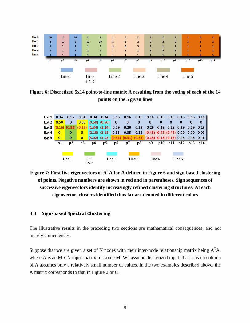
8
Figure 6: Discretized 5x14 point-to-line matrix A resulting from the voting of each of the 14 points on the 5 given lines
Figure 7: First five eigenvectors of ATA for A defined in Figure 6 and sign-based clustering of points. Negative numbers are shown in red and in parentheses. Sign sequences of successive eigenvectors identify increasingly refined clustering structures. At each
eigenvector, clusters identified thus far are denoted in different colors
3.3 Signbased Spectral Clustering
The illustrative results in the preceding two sections are mathematical consequences, and not merely coincidences. Suppose that we are given a set of N nodes with their inter-node relationship matrix being ATA, where A is an M x N input matrix for some M. We assume discretized input, that is, each column of A assumes only a relatively small number of values. In the two examples described above, the A matrix corresponds to that in Figure 2 or 6.

9
We formally define what we mean by clusters. A subset of nodes are said to form a cluster if they are “essentially indistinguishable,” in the sense that for each eigenvector of ATA, these nodes assume the same sign. That is, for any given eigenvector, its components for these nodes are either all positive or negative or zero. Note that under this definition clusters can be more flexibly defined than clusters defined as containing “truly indistinguishable” nodes in the sense that they actually assume the same component value in each eigenvector, beyond just the same sign. Consider, for example, Figure 4. We see that under our definition, sensors 0 through 5 form a cluster because they assume the same sign (not their values) for each of the three eigenvectors. If we used value-based clustering, this cluster would have to be broken into three clusters: sensors 0-1, 2-3 and 4-5. Clustering at this fine granularity could be misleading when inputs are subject to certain degrees of uncertainty. By our definition of clustering, for any two given clusters, at least one eigenvector will assume different signs on the two clusters. This means that sign sequences from all the eigenvectors can always identify all the clusters. However, we can expect a stronger result. That is, suppose sign-based spectral clustering uses any k eigenvectors of ATA, including the principal eigenvector, for any k from 2 through the rank of ATA. Then these k eigenvectors will exhibit at least k distinct sign sequences, thereby being able to identify at least k cluster groups, where a cluster group is composed of a single cluster or multiple of them.
3.4 Modeling Expected Measurement Consistency of Sensors
We formalize the expectation that those sensors which have similar sensing and system characteristics and are situated in close proximity with a similar environment will report similar measurement data. To this end, we use “sensor indexing”to capture these similarities in sensors. More precisely, we summarize below some important concepts, assumptions and terms:
There are a number of reference targets ti, or simply targets, on which sensors sj report measurements. We call the measurements of a sensor on a target the weight for this sensor-target pair.
Sensors can be clustered based on their measurements, so a cluster contains those sensors which report similar measurements. We call these clusters measurement clusters.
Sensors can be mapped into an index space. Peer sensors or simply peers, are those which have nearby indices according to some distance metric for index pairs.
Sensors can be clustered based on their indices so a cluster contains sensors with nearby indices, i.e., peer sensors. We call these clusters peer clusters.

10
It is assumed that the indexing scheme satisfies the property that peer sensors will report similar measurements on the targets. Moreover, for any given measurement cluster, there is a corresponding peer cluster, and vice versa.
It is assumed that each sensor has sufficiently many peers. A sensor whose measurement and peer clusters coincide is called a good sensor.
Otherwise the sensor is called a bad sensor. Choosing a proper granularity of measurement clusters (and the corresponding peer clusters) is a design choice. One may divide a measurement cluster into smaller ones, by recognizing finer measurement differences among sensors. For example, when using sign-based spectral clustering, we can examine additional leading eigenvectors for finer measurement clustering. Generally speaking, based on finer-grain measurement clusters, we can increase the success rate of catching bad nodes, but possibly at the expense of more false positives. After a certain point, decreasing the cluster size will have diminishing returns. When this point is reached, we may use other methods of identifying additional bad sensors without decreasing cluster sizes. For example, we can identify sensors on the edge of a measurement cluster as bad sensors. To illustrate this concept of sensor indexing, we consider a simple example described in [3], where the sensor property utilized as the sensor index is the sensors’ antenna polarization angle. In this case, peer sensors are those which have similar antenna polarizations. Suppose that the received signal strength (RSS) values reported by a sensor on some target correlate with the matching degree of the antenna polarizations of the sensor and the target. Then, those peer sensors which are in good working conditions are expected to report similar RSS measurements on the same targets. Like granularity of measurement clusters, choosing a proper sensor indexing scheme is a design choice. For a given sensor-based application the indexing scheme should be related to sensing metrics used so peer sensors can be expected to perform similarly for the application. For example, for a two-dimensional (2D) localization application using radio frequency (RF) ranging measurements, it would be appropriate to index sensors based on their 2D geographical locations.

11
Next, we describe our spectral-based method for forming measurement clusters of sensors and how we use these sensor clusters to identify bad sensors. We will first form a measurement matrix A where entry aij of A is the measurement weight for the sensor-target pair (sj , ti) defined in the beginning of this subsection. We will then perform spectral analysis on ATA, since the eigenvectors of ATA characterize similarities among sensors in their measurement data. Based on the eigenvectors of ATA, we will cluster sensor nodes using methods such as sign-based clustering. From the above, it follows that, to identify bad sensors, we will form the measurement cluster to which a sensor belongs, and then determine if the measurement cluster agrees with the corresponding peer cluster. We assume that there are plentiful sensors so that each sensor has a sufficient number of peers for the bad sensors identification method. It follows from the above discussion that a sensor is deemed to be bad if the sensor satisfies one of the two conditions: (C1) the sensor is in a small unique measurement cluster, or
(C2) the sensor is in a small out-of-place component (in the index space) of a measurement cluster.
Therefore the essence of the clustering problem studied here is to identify these two conditions for sensors. We show that we can achieve this objective by examining leading eigenvectors of ATA.

12
4.0 RESULTS AND DISCUSSION
4.1 Performance Comparisons for Signbased Spectral Clustering
In this section we present a qualitative comparison of the performance of sign-based spectral clustering to a state-of-the-art k-means-based spectral clustering. As we will see, the sign-based clustering, in spite of being simpler and faster, can perform comparably to more complex techniques.
4.1.1 Related Work on KMeans
A number of previous works have applied spectral techniques to deduce clustering in data of interest. In general, such works share the approach of first obtaining eigenvectors of some data relationship matrix, and then using some custom technique to compute clusters from the eigenvectors. For example, in an early work on image segmentation [5], researchers partitioned the input data repeatedly based on the values of the elements in the second eigenvector; the resulting recursive clustering was thus hierarchical. Subsequent work improved upon this by considering the top k eigenvectors of the data relationship matrix, instead of just the second. In particular, Ng et al. [6] applied the standard k-means clustering technique [10] to points in k-dimensional space whose coordinates are the respective elements of the top k eigenvectors. Applying k-means clustering to a low-dimensional eigenbasis instead of the input data directly allowed it to perform significantly better. The heuristic algorithms used to implement k-means clustering have various limitations, such as a potentially superpolynomial running time [7], sensitivity to initial values, or the inability to automatically deduce the number of clusters. While researchers have tried to address some of these limitations in follow-on works, the solutions remain relatively complex [11].

13
The sign-based spectral clustering studied in this work is a simple alternative to the k-means-based clustering algorithms; in particular, it does not depend on initial values, and does not require multiple iterations; in fact, after the eigenvectors are computed, its run-time of O(Nd) is favorable to the O(Ndk) run-time [7] of a k-means iteration, where N is the number of data objects, d number of feature dimensions per object, and k number of clusters requested from the algorithm. Note that O(Nd) or O(Ndk) corresponds to the size of the data set that the sign-based spectral clustering or a k-means iteration needs to examine, respectively. The number of iterations k-means requires can be large and unpredictable, especially when the number of clusters is not known a priori, and as a result, an incorrect number of clusters is input to the algorithm.
4.1.2 Test Scenario
We use a simple 4-line scenario to compare k-means and sign-based clustering, depicted in Figure 8. We assume that there are 900 sensors placed in a 30 × 30 grid surrounding the 4 line segments. We further model a sensor’s measurement of a particular line by an inverse-square function of the sensor’s distance from the nearest point on the line. Thus, based on these measurements we form a 4 x 900 measurement matrix A. Lastly, for discretized cases we use a simple bi-level step function where sensors closer to the line than a threshold distance of 0.5 attain a measurement magnitude 1.0, and 0.01 otherwise.
Figure 8. Scenario used to compare sign-based and k-means clustering

14
4.1.3 Performance Comparison in Robustness and Speed
We compare the performances of k-means-based and sign-based spectral clustering on raw and discretized inputs. The outcomes of the 4 possible scenarios appear in Figure 9. As we can see in Figure 9b, without discretization the sign-based clustering obtains a far worse solution than k-means, misclassifying a whole diamond-shaped region of the background together with the points near a target line. However, with discretization, sign-based clustering finds an accurate solution. The solution, shown in Figure 9d, is comparable to k-means solutions. More precisely, we see that there are 6 sign-based clusters identified, corresponding to the 6 region colors in Figure 9d. Under the given discretization, a sensor's measurement of a line assumes only one of the two values 1 or 0.01. Suppose that we partition nodes into equivalence sets by including in the same set those nodes which assume the same measurement value for each of the four target lines. Then there are only a total of 9 equivalence sets: four line stripes, four intersection blocks and one remaining background region. Nodes in the same equivalent must belong to the same sign-based cluster. We see that the four eigenvectors of ATA have identified 6 these equivalence sets. The three left out are the ones corresponding to the smallest equivalence sets which are intersection blocks.
Figure 9: A comparison of clustering outcomes under sign-based and k-means clustering, and with or without discretized input weights

15
4.2 Validating Sensors in the Field via Spectral Clustering
4.2.1 Simulation Results on Large Systems
In this section, we present simulation results on the model application with 400 sensors. We assume that the sensors are evenly partitioned into four groups of 100. We further assume that some randomly selected sensors are bad sensors, in the sense that all their measurements of other sensors have a random measurement error α~ N(μbad ,σbad). That is, if the true measurement for a sensor-target pair is w, then the observed one isαw. We used the error parametersμbad = 10 andσbad = 3.2. For all other links where both transmitting and receiving sensors are good, we omitted the error term; that is, μgood = 0 andσgood = 0. The purpose of the simulation is to assess the effectiveness of our spectral clustering method in identifying these bad sensors. In the simulation, there are 50 bad sensors. Let B be the ground truth number of bad sensors input to the simulator, T the total number of sensors deemed as bad sensors by our clustering method, and B* the number of sensors that the clustering method correctly identified as bad. Hence, B* ≦ B and B* ≦ T. The higher the detection rate B*/B is, the better the method is. Note that T – B* is the number of false positives. We are interested in raising the detection rate B*/B, without raising the false positive rate (T – B*)/T significantly. But usually there is a tradeoff between the two factors. We study performance under varying numbers k of leading eigenvectors used in the spectral clustering method. In the simulator we assume that the minimum cluster size Smin = 2. Meanwhile, we explore a range of values for the parameter τ, or the fraction of sensors furthest from a cluster center which we will declare bad. Increasingτleads to identifying more bad nodes, but usually at the expense of more false positives. The following observation supported by simulation results (see Figure 12) is worth mentioning. Before a certain threshold (e.g., 6) on the number k of leading eigenvectors used in spectral clustering is reached, when we increase k, we can catch more bad sensors while keeping theτ
value constant. This means that by increasing k, we can increase the bad sensor detection rate, without increasing the false positive rate. This result follows from the fact that use of more eigenvectors (before reaching some threshold on k) will give finer-grained measurement clusters, which in turn will allow us to identify bad sensors which have smaller errors in their computed locations.

16
Figures 10 and 11 show results on two performance metrics: the bad sensor detection rate and false positive rate, respectively, with respect to theτthreshold. Additionally, Figure 12 shows the effect of the number k of leading eigenvectors used on detection and false positive rates. We note the following from the figures: 1) When k increases, the detection performance improves for each value of τ. When k is at
its highest value of 14, the best performance is achieved (see Figure 10). 2) For certain values of k, the false positive rates as a function of τexhibit a minimum; in
Figure 11 these minimums are reached around τ= 10% to 15%. 3) For a fixedτ, there are values of k which give minimal false positive rates; for example, for
τ= 10%, the lowest false positive rate in Figure 12 is reached for k = 6. 4) Increasing k past that giving the minimum false positive rate only provides a minor increase
in detection rate. Given that the false positive rate increases rapidly, the best value for k is close to the number of major sensor clusters, or, equivalently, the number of leading eigenvalues significantly larger than the rest.
Figure 10: Number of bad sensors, out of 50, identified for increasing values of parameterτ and a range of values for the number of leading eigenvectors k used for spectral
clustering

17
Figure 11: False positive rate of the spectral clustering method under increasing
threshold τ, for a range of number k of leading eigenvectors used for spectral clustering
Figure 12: Detection rate and false positive rate plotted against number k of leading
eigenvectors used for spectral clustering for three representative values ofτ

18
5.0 CONCLUSIONS
5.1 Signbased Spectral Clustering
Sign-based spectral clustering gives an accurate classification of discrete input which is amenable to clear data separation. It is simple, fast and robust. There is no need to use heuristics in searching for clusters. With the use of an increasing number of eigenvectors sign-based clustering can reveal clustering structures at increasingly refined granularity.
5.2 Validating Sensors in the Field via Spectral Clustering
We have described a new method of using leading eigenvectors in forming measurement clusters of sensors. Although spectral-based clustering is well known in the literature [15], our use in validating sensors in the field appears to be novel. More specifically, to the best of our knowledge, our formulation of sensor indexing and our method of identifying bad sensors using conditions C1 and C2 are new. As shown in our simulation experiments, the method can identify bad sensors with high accuracy and low false positive rate. The sensor validation methodology described here is general, and opens up a number of avenues of future work. For instance, there is the question of which specific sensor properties to use for indexing. In addition to the straightforward ones such as those we used, there might be additional ones based on other sensor modalities, or certain transforms of the sensing data such as the Hough transform [8]. Secondly, there are potentially many other sensor-based applications which can benefit from the proposed sensor validation approach such as cognitive radio spectrum allocation.

19
6.0 REFERENCES
1. S. White and P. Smyth, “A spectral clustering approach to finding communities in graphs,” in
SIAM International Conference on Data Mining, 2005. 2. D. Higham, G. Kalna, and M. Kibble, “Spectral clustering and its use in bioinformatics,”
Journal of Computational and Applied Mathematics, vol. 204, no. 1, pp. 25–37, July 2007. 3. M. Kurucz, A. Bencz´ur, K. Csalog´any, and L. Luk´acs, “Spectral Clustering in Telephone
Call Graphs,” in Proceedings of the Joint 9th WEBKDD and 1st SNA-KDD Workshop, 2007.
4. S. Foucher and L. Gagnon, “Automatic detection and clustering of actor faces based on spectral clustering techniques,” in CRV ’07: Proceedings of the Fourth Canadian Conference on Computer and Robot Vision. Washington, DC, USA: IEEE Computer Society, 2007, pp. 113–122.
5. J. Shi and J. Malik, “Normalized cuts and image segmentation,” in IEEE Conf. Computer Vision and Pattern Recognition, Jun. 1997.
6. A. Y. Ng, M. I. Jordan, and Y. Weiss, “On spectral clustering: Analysis and an algorithm,” in Advances in Neural Information Processing Systems (NIPS) 14, 2002.
7. D. Arthur and S. Vassilvitskii, “On the worst case complexity of the k-means method,” in 22nd Annual ACM Symposium on Computational Geometry, 2006.
8. R. O. Duda and P. E. Hart, “Use of the Hough Transformation to Detect Lines and Curves in Pictures,” Communications of the ACM, pp. 11–15, Jan. 1972.
9. A. Berman and R. J. Plemmons, Nonnegative Matrices in the Mathematical Sciences. New York, NY: Academic Press, 1979.
10. J. B. MacQueen, “Some methods for classification and analysis of multivariate observations,” in Proceedings of 5th Berkeley Symposium on Mathematical Statistics and Probability, Berkeley, CA, USA, 1967, pp. 281–297.
11. L. Zelnik-Manor and P. Perona, “Self-tuning spectral clustering,” in In Advances in Neural Information Processing Systems (NIPS) 17, 2005.
12. H. T. Kung and D. Vlah, “A Spectral Clustering Approach to Validating Sensors via Their Peers in Distributed Sensor Networks,” in Second International Workshop on Sensor Networks (SN2009), San Francisco, CA, Aug. 2009.
13. H. T. and D. Vlah, “Validating Sensors in the Field via Spectral Clustering Based on Their Measurement Data,” in Military Communications Conference (MILCOM 2009), Boston, MA, Oct. 2009
14. H. T. Kung, C. K. Lin, T. H. Lin, and D. Vlah, “Localization with Snap-Inducing Shaped

20
Residuals (SISR): Coping with Errors in Measurement,” in the 15th Annual International Conference on Mobile Computing and Networking, Beijing, China, Sep. 2009.
15. A. Y. Ng, M. I. Jordan, and Y. Weiss, “On spectral clustering: Analysis and an algorithm,” in Advances in Neural Information Processing Systems 14. MIT Press, 2001, pp. 849–856.
16. Y. Shang, W. Ruml, Y. Zhang, and M. Fromherz, “Localization from connectivity in sensor networks,” Parallel and Distributed Systems, IEEE Transactions on, vol. 15, no. 11, pp. 961–974, 2004.

21
7.0 LIST OF SYMBOLS, ABBREVIATIONS, AND ACRONYMS
K-Mean K-means clustering is a well-known algorithm to classify or to group objects
based on attributes/features into K number of groups MDS Multi-Dimensional Scaling RSS Received Signal Strength SISR Snap-Inducing Shaped Residuals