POLITECNICO DI MILANO

Ingegneria dei SistemiCorso di Laurea in Ingegneria Biomedica

Fluid-structure interactionsimulations of hemodynamics in mice:applications to hypertension research

Relatore:Prof. Francesco Migliavacca

Correlatore:Prof. C. Alberto Figueroa

Candidata:Federica Cuomo

765319

Anno Accademico 2012-2013

Contents

1 Introduction 201.1 Clinical motivation . . . . . . . . . . . . . . . . . . . . . . . . 201.2 The big picture . . . . . . . . . . . . . . . . . . . . . . . . . . 221.3 Computational Fluid Dynamics framework . . . . . . . . . . . 23

1.3.1 Outflow boundary conditions . . . . . . . . . . . . . . 25

2 Methods 272.1 Data research in literature . . . . . . . . . . . . . . . . . . . . 27

2.1.1 Flow data . . . . . . . . . . . . . . . . . . . . . . . . . 272.1.2 Pressure data . . . . . . . . . . . . . . . . . . . . . . . 302.1.3 Geometrical data . . . . . . . . . . . . . . . . . . . . . 37

2.2 Building the 3D geometric mouse model . . . . . . . . . . . . 422.2.1 Original geometry . . . . . . . . . . . . . . . . . . . . . 422.2.2 Up-scaled model . . . . . . . . . . . . . . . . . . . . . 432.2.3 Intercostal arteries . . . . . . . . . . . . . . . . . . . . 46

2.3 Computational fluid dynamics method . . . . . . . . . . . . . 472.3.1 Mesh and mesh adaptivity . . . . . . . . . . . . . . . . 472.3.2 Multiscale modelling approach . . . . . . . . . . . . . . 472.3.3 Fluid-structure interaction . . . . . . . . . . . . . . . . 512.3.4 Tissue support . . . . . . . . . . . . . . . . . . . . . . 52

2.4 Boundary condition specification . . . . . . . . . . . . . . . . 53

3 Results 573.0.1 Baseline model . . . . . . . . . . . . . . . . . . . . . . 573.0.2 Modified distal compliance case . . . . . . . . . . . . . 613.0.3 Increased arterial stiffness . . . . . . . . . . . . . . . . 61

4 Discussion 66

2

List of Figures

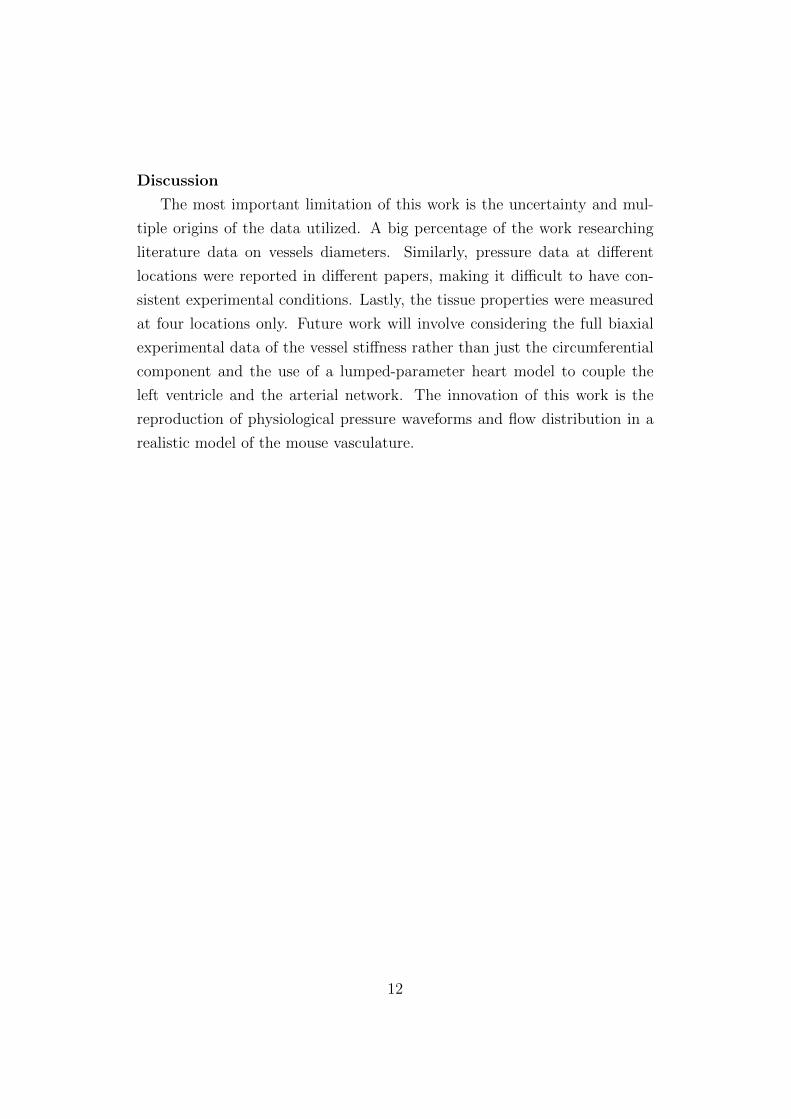
1 Pressure simulation at seven different location along the aortaand flow waveforms compared to literature data at represen-tative locations. . . . . . . . . . . . . . . . . . . . . . . . . . . 13

2 Pressione risultante in sette diverse posizioni lungo l’aorta eonde di flusso in posizioni rappresentative confrontato ai datiriportati in litteratura. . . . . . . . . . . . . . . . . . . . . . . 19

1.1 Propagation of the pulse pressure (PP) wave from central toperipheral arteries in adult humans aged 24, 54 and 68 years.[1] . . . . . . . . . . . . . . . . . . . . . . . . . . . . . . . . . 21

1.2 Tipical boundaries of a fluid domain in hemodynamics . . . . 241.3 Three-element Windkessel model . . . . . . . . . . . . . . . . 26

2.1 Flow waveform in ascending aorta reported in Lujan t al. [2] . 292.2 Average inflow signal obtaine from the Lujan data. . . . . . . 302.3 Flow data in innominate artery and left common carotid cal-

culated from high-resolution magnetic resonance reported inFeintuch et al. Feintuch et al. [3] . . . . . . . . . . . . . . . . 31

2.4 Flow data in the infra-renal abdominal aorta, Greve et al. [4] . 322.5 Path along the aorta and 2-D segmentations of the vessel lumen. 432.6 Lateral, anterior, and axial views of the 3D Model built from

the micro-CT imaging of the corrosion cast . . . . . . . . . . . 442.7 View of the original geometry (inner) and the upscaled geom-

etry (external overlay). . . . . . . . . . . . . . . . . . . . . . . 452.8 Partial view of the mesh after mesh adaptivity. . . . . . . . . . 482.9 The overall fluid domain Ω is separated into an upstream nu-

merical domain Ω and a downstream analytical domain Ω′,demarcated by the interface Γout. . . . . . . . . . . . . . . . . 50

2.10 Biaxial stiffness values in four different location measured atin vivo axial stretch λ and pressure=100mmHg. . . . . . . . . 53

3

2.11 Tissue properties: young modulus interpolated from the dataacquired at Professor Humphrey’s lab and thickness definedas 10% of the local radius. . . . . . . . . . . . . . . . . . . . . 54

3.1 Magnitude of the wall shear stress, volume rendering of thevelocity magnitude and pressure at the peak systolic. . . . . . 59

3.2 Flow waveforms compared to literature data at representativelocations in the model . . . . . . . . . . . . . . . . . . . . . . 60

3.3 Pressure waveform at different locations in the aorta. . . . . . 623.4 Pressure pulse propagation along the aorta for the baseline

(left) and decreased peripheral compliance (right). . . . . . . . 633.5 Pressure waveform in different location along the aorta in three

different cases with increased levels of arterial stiffness. . . . . 64

4.1 Cross sectional flow waveform in the ascending aorta: the datafrom Feintuch shows diastolic back flow. . . . . . . . . . . . . 67

4

List of Tables

2.1 Iliac artery pressure measurements, Reddy et al. [5]. . . . . . . 342.2 Pressures in the aortic root measured through implantable

catheter Reddy et al. [6]. . . . . . . . . . . . . . . . . . . . . . 352.3 Blood pressure in the aortic arch measured through radio

telemetry systems, Van Vliet et al. [7] . . . . . . . . . . . . . 362.4 Blood pressure in the aortic arch measured through radio

telemetry systems, McGuire et al. [8] . . . . . . . . . . . . . . 362.5 Comparison of diameters obtained with casting and in vivo

micro-CT, Vandeghinste et al. [9] . . . . . . . . . . . . . . . . 382.6 Vessel diameter measurements obtained by Casteleyn et al. [10] 392.7 Aortic root and ascending aorta diameters, Hinton et al. [11] . 392.8 Carotid diameters obtained via biaxial tissue testing by Wan

et al. [12] . . . . . . . . . . . . . . . . . . . . . . . . . . . . . 402.9 Mean diameters reported by Trachet et al. [13]. BW: body

weight, HR: heart rate, PAA: proximal abdominal aorta, CEL: celiac artery, MES: mesenteric artery, RREN: right renalartery, LREN: left renal artery, DAA: distal abdominal artery.The diameters are reported in mm. . . . . . . . . . . . . . . . 40

2.10 The location, the diameter of the model and the diameterof the best reference are reported. AAo: ascending aorta,AA: aortic arch, DA: descending aorta, IN: innominate artery,LCC: left common carotid, LSUB: left subclavian, CEL: celiacartery, MES: mesenteric artery, RREN: right renal artery,LREN: left renal artery. Measurements reported in mm. . . . 41

2.11 Fractional longitudinal position of the intercostals on branchvessel along the aorta, Guo et al. [14] . . . . . . . . . . . . . . 46

3.1 Windkessel parameters in the baseline simulation. The resis-

tances are expressed inPa · smm3

and the compliance in 10−6mm3

Pa. 58

3.2 Simulated and reference values of %CO . . . . . . . . . . . . . 58

5

3.3 Pulse wave velocity (PWV) in three cases with increased stiff-ness. . . . . . . . . . . . . . . . . . . . . . . . . . . . . . . . . 65

6

Acknowledgments

This work was carried out at King’s college London, in Prof. Figueroa’s lab.

It is the outcome of an unforgettable experience.

I would like to express my deepest thanks to my supervisor, Prof. C. Al-

berto Figueroa, for the incomparable opportunity granted by accepting me

into his lab. I thank him for the immense effort he put into training me in

both scientific and non-scientific field, for his constant guidance, support and

encouragement and for showing me every day what passion and devotion to

doing something means.

My sincere gratitude goes to Prof. Francesco Migliavacca for his role in

making this experience possible, and for his enduring support.

I’m also thankful to Kevs (Kevin Lao), Nan (Xiao) and Des (Desmond

Dillon Murphy), who have been there sustaining me from day one, for their

care, for their precious friendship, and for their irreplaceable and constant

help. Together with Ed (Edward Evans), Alia (Noorani) and Chris (Christo-

pher Arthurs), they made jokes and laughing easy at every moment. I

couldn’t desire a better group; I learned something from every one of you.

Un grazie di cuore va ai miei adorati genitori, per avermi incoraggiata,

supportata e sopportata dal primo giorno di universita all’ultimo giorno di

tesi; per non avermi mai negato nuove esperienze e per averle rese possibili.

7

Abstract

Motivation

Arterial stiffening is both cause and consequence of hypertension,currently

the main cause of death in Europe. Hemodynamic metrics such as central

pulse pressure (cPP) and pulse wave velocity, which can be non invasively

measured, are now known as important predictive factors of diseases and

diseases susceptibility. Computational Fluid Dymanic techniques enable an

accurate representation of hemodynamics in the central arteries, hence pro-

viding a non-invasive estimate of the time varying pressure and flow. These

techniques, combined with experimental and imaging data are fundamen-

tal in understanding the correlation between arterial stiffness and hemody-

namics. Computational simulations can provide improved interpretations of

clinically measurable metrics of pulse wave velocity and even identify new

metrics based on pressure waveform analysis. The objective of this work is

to validate a new computational biomechanical fluid-solid interaction tool in

a mouse model. This tool employs a Fluid Structure Interaction (FSI) tech-

nique to represent the deformability of the wall vessel which is fundamental

to capture pulse pressure propagation. It also uses a multi-domain method

to include the impact of distal vasculatures in the aortic geometry, as it well

known that distal vessels have a remarkable influence on the hemodynamics

of the central arteries.

Methods

We set out to search reliable flow, pressure and geometrical data in mice

to use both as input data and as results validation. In vivo measurements

in mice are challenging due to the small dimension of the body and the fast

8

heart rate. The data used in the simulations have been carefully chosen to

ensure consistency between weight, age and strain of the mice tested. Con-

sidering this, we found references for flow data in ascending aorta, left com-

mon carotid, innominate artery and infra-renal abdominal artery; systolic,

diastolic and mean pressure values in the aortic arch; and vessel diameter di-

mensions for three locations along the aorta and for renal, mesenteric, celiac,

left common carotid, subclavian and innominate arteries. An initial 3-D geo-

metrical model was built from micro-CT imaging of a vascular casting using

the custom software Simvascular. The model included ascending, descend-

ing and abdominal aorta plus significant segments of subclavians, carotids,

renal arteries, mesenteric, celiac and tail. The vascular casting technique,

performed at Biomedical Department of Yale University, resulted in geom-

etry with smaller than physiological diameters. This geometry resulted in

highly unrealistic pressures when pulsing physiological levels of flow, due to

the artificially large resistance of the model. Therefore the initial geometry

was upscaled to match the diameter data found in literature. The initial

model did not represent the intercostal vessels, as they are too narrow to be

captured by either imaging. Since these vessels carry a significant amount of

flow, nine pairs of intercostal arteries were added along the thoracic aorta of

the model.

Once the model was ready, a finite element mesh was obtained in Simvascular

and a first simulation was run with rigid walls; followed by a gradient-based

mesh adaptivity technique. This technique took into account the distribution

of velocity gradients of the previous simulation to obtain a uniform distribu-

tion of the error in all special directions.

The computational fluid dynamics method used relies on a multi-scale mod-

eling approach, whereby a decomposition of the spatial domain and of the

variables is introduced. Within this approach two domains coexist: a nu-

merical domain in which the Navier-Stokes equations for an incompressible

Newtonian fluid are solved and an analytic domain in which a lumped param-

eter formulation is employed. In our case the numerical domain was the 3-D

geometrical model of the central arteries and the major branches, while the

three-elements Windkessel models were adopted to represent the distal ves-

9

sels until the capillaries level. The Windkessel model is an electrical circuite

analogue of the circulation: it consists of a proximal resistance connected in

series with a parallel of a distal resistance and a compliance. Onece a three-

element Windkessel model is coupled at each outlet of the 3-D domain, a

model with large number of vessels, as ours, requires the specification of nu-

merous parameters. A systematic approach to obtain the parameters based

on 1D-theory [15], was adopted in this work. Briefly, the total resistance

of the model (combination of 3-D and 0-D) was calculated by taking into

account the mean value of the flow at the inlet and target mean pressure.

The resistance of the 3-D geometry was then assumed to be zero, since the

contribution of the central arteries to the total resistance is much smaller

than that of the distal circulation. The total resistance for each outlets was

split between proximal and distal resistances. The proximal resistance was

calculated to match the characteristic impedance of the correspondent outlet

of the upstream domain. A similar approach was adopted to evaluate the

compliance values: a total arterial compliance was first calculated. Unlike

with the resistance, the contribution of the central arteries to the total ar-

terial compliance can not be assumed equal to zero. We thus estimated the

compliance of the central arteries as the sum of the compliance of each ves-

sel. Lastly, the peripheral compliance which was then distributed among the

different outlets in proportion to the flow distribution.

The computational fluid dynamic method adopted in this work also includes

a fluid-structure interaction technique. This aspect is fundamental in order to

capture pulse pressure propagation in the contest of arterial stiffening and hy-

pertension. The FSI ”Coupled Momentum” method developed by Figueroa

and Taylor at Stanford was used [16]. Here, the elastodynamic equations

representing the deformation of the wall are incorporated in the stabilized

finite element formulation of the Navier-Stokes equations and a traction field

describing the wall behavior is applied as boundary condition to the lateral

boundary of the fluid domain. The vessel wall is modeled as a linear elastic

membrane characterized by a young modulus E, a Poisson ratio ν = 0.5, and

a thickness h. Variable tissue properties were considered in this thesis. The

thickness h was estimated as 10% of the local radius according to literature

10

data [1]. Experimental stiffness values were obtained at the Department of

Biomedical Engineering of Yale University. Stiffness data measured at four

different locations were interpolated throughout the model. The support of

the perivascular tissue and other organs on the vessels was also modeled as

a traction acting on the outer boundary of the arterial wall.

Results

Four simulations were performed: a baseline case, a case with reduced

distal compliance values and two cases with increased vessel stiffness in the

central vessel. A representative ascending aortic flow waveform acquired from

Lujan et al. [2] was prescribed. The average cardiac output was 11.92 ml/min

and the cardiac cycle 0.147 s. The flow distribution obtained in the baseline

case was in good agreement with literature data [3] [4], even though there

are some qualitative differences in the shape of the waveforms (see Figure

1). This incongruity is probably due to the lack of diastolic backflow in the

ascending aorta flow data considered[3]; and also ndue to the need for further

tunning of the outflow boundary condition parameters. On the other hand

the shape and range of the pressure waveform correspond well to the known

physiological behavior [17]. As reported in literature, no pulse pressure am-

plification along the aorta is observed in mice. This is in contrast with what

happens in young humans. The pressure in the ascending aorta ranged from

93 to 120 mmHg, while in the infra-renal abdominal aorta the range was 93

to 113 mmHg (see Figure 1). In the interest of investigating whether the

amplification of the pulse is obtainable in mice geometry, the RCR values

of the baseline case were modified by decreasing the compliance of the lower

vessels. Under these conditions, augmentation of the pulse pressure down

the aorta was obtained. The effects of augmented arterial stiffness due to

aging and hypertension were also examined. Two simulations were set up

with adifferent distributions of elastic modulus E (increased by a factor of 2

and 3 relative to the baseline, respectively). In both cases, the pulse pres-

sure and pulse wave velocity increased along the aorta with higher stiffness

as reported in literature [6].

11

Discussion

The most important limitation of this work is the uncertainty and mul-

tiple origins of the data utilized. A big percentage of the work researching

literature data on vessels diameters. Similarly, pressure data at different

locations were reported in different papers, making it difficult to have con-

sistent experimental conditions. Lastly, the tissue properties were measured

at four locations only. Future work will involve considering the full biaxial

experimental data of the vessel stiffness rather than just the circumferential

component and the use of a lumped-parameter heart model to couple the

left ventricle and the arterial network. The innovation of this work is the

reproduction of physiological pressure waveforms and flow distribution in a

realistic model of the mouse vasculature.

12

1 2

3

4

5

6

7

27 m

mHg

147 ms

20 m

mH

g

1

2

3

4

5

6

7

-1

2

5

8

11

0 50 100 150

Flow

(ml/

min

)

Time (ms)

-1

2

5

8

0 50 100 150

Flow

(ml/

min

)

Time (ms)

-1

2

5

8

11

0 50 100 150

Flow

(ml/

min

)

Time (ms)

Simulation

Feintuch et al.

Greve et al.

Figure 1: Pressure simulation at seven different location along the aorta andflow waveforms compared to literature data at representative locations.

13

Sommario

Introduzione

Le malattie cardiovascolari sono la principale causa di morte in Europa.

L’irrigidamento delle arterie e oggigiorno riconsciuto come causa e conse-

quenza dell’ipertensione che e uno dei principali fattori di rischio per le

malattie cardiovascolari. Il polso pressorio e la sua velocita sono misurabili

tramite procedure non invasive e sono ritenuti importanti fattori predittivi

di eventi cardiovascolari. Vi e necessita di capire come i cambiamenti della

rigidezza arteriosa influenzino localmente e globalmente l’emodinamica. In

questo contesto diventano sempre piu’ importanti gli studi computazionali

che permettono una riproduzione accurata e realistica di grandezze emod-

inamiche, fornendo una stima accurata e non invasiva dell’onda pressoria.

L’obiettivo di questo lavoro e validare un nuovo strumento di biomeccanica

computazionale della anatomia del topo. Un metodo d’interazione fluido-

struttura e stato utilizzato per includere la deformabilita delle pareti dei vasi

nell’analisi della propagazione del polso pressorio. Un approccio multi-scala e

stato applicato per includere i vasi distali, fino a livello dei capillari, nel mod-

ello siccome la rete arteriosa distale ha una forte influenza sull’emodinamica

delle arterie centrali.

Metodi

Una componente molto importante del lavoro e stata la ricerca in let-

teratura di dati affidabili riguardanti il flusso sanguigno, la pressione e le

dimensioni dei vasi nei topi. Le misurazioni in vivo sono rese difficili dalle ri-

dotti dimensioni dell’anatomia e dall’alta frequenza cardica (circa 600bpm) di

questi animali. I dati sono stati attentamente scelti, essendo a conoscenza dei

14

limiti e dei vantaggi delle tecnologie attualmente in uso e mantenedo coerenza

tra il peso, l’eta e la tipologia del topo. Le grandezze di riferimento prese

in considerazione sono: la variazione del flusso nel tempo nell’aorta as-

cendente, nell’arteria carotidea comune, innominata, e nell’aorta addominale

sottorenale, i valori di pressione media, sistolica e diastolica misurati

nell’arco aortico ed il diametro dell’aorta (3 diverse posizioni), dell’arteria

renale, mesenterica, celiaca, carotidea comune, succlavia e innominata.

Dalle immagini micro-CT di un campione ottenuto tramite la tecnica di vas-

cular corrosion casting e stato costruito il modello geometrico tridimensionale

utilizzando il software Simvascular. La procedura di corrosion casting e stata

eseguita nel dipartimento di Biomedica dell’Universita di Yale. Poiche il mod-

ello risultante sottostimava la geometria reale, i valori di pressione stimati

dalle simulazioni risultavano maggiori di quelli fisiologici. Per questo motivo

le dimensioni del modello geometrico sono state aumentate per riprodurre i

valori dei diametri trovati in letteratura. Il modello originale comprendeva

l’aorta ascendente, discendente e addominale oltre a segmenti delle arterie

succlavia, carotidee, renali, mesenterica, celiaca e l’arteria della coda. Il mod-

ello originale non considerava le arterie intercostali, troppo piccole per poter

essere visualizzate nelle immagini. Poiche in questi vasi scorre una parte

importante della gittata cardiaca, nove paia di arterie intercostali sono state

aggiunte alla geometria lungo l’aorta toracica.

La mesh del modello e stata ottenuta usando la libreria di Simvascular ed

una prima simulazione con pareti rigide e stata eseguita ed in base ai risultati

la mesh e stata adattata tenendo in considerazione la distribuzione del gradi-

ente di velocita, per ottenere una distribuzione uniforme in tutte le direzioni.

Al fine di eseguire diversi livelli di modellizazione, e stata utilizzato un ap-

proccio multi-scala che comprende una decomposizione del dominio e delle

variabili. L’approccio multi-scala suddivide il dominio in un dominio nu-

merico, in cui vengono risolte le equazioni di Navier-Stokes per un fluido

newtoniano incomprimibile, ed un dominio analitico, in cui viene adottata

una formulazione a parametri concentrati. Nel nostro caso, il modello tridi-

mensionale delle arterie centrali e delle prinicpali diramazioni e il dominio

numerico, mentre un modello Windkessel a tre elementi e stato impiegato

15

come dominio analitico per rappresentare i vasi distali fino a livello dei capil-

lari. Il modello Windkessel e un analogo elettrico della circolazione sanguigna

costituito da una resistenza prossimale in serie al parallelo di una resistenza

distale ed un condensatore (RCR). Un modello Windkessl a tre elementi e

accoppiato ad ogni vaso del modello tridimensionale; una geometria comp-

lessa con un numero elevato di diramazioni richiede quindi la specificazione di

molti parametri. In questo lavoro e stato adottato un approccio basato sulla

teoria 1-D [15] per ottenere i valori di questi parametri in modo sistematico.

Brevemente, una resistenza assegnata a tutto il modello (combinazione della

parte 3-D e della parte 1-D) e stata calcolata considerando il valore medio del

flusso prescritto a livello dell’aorta ascendente e la pressione media desider-

ata. La resistenza rappresentata dal modello 3-D e stata considerata nulla,

poiche il contributo delle arterie centrali e decisamente inferiore rispetto alla

componente distale. La resistanza totale e stata quindi partizionata tra le

resistanze prossimali e distali di ogni modello Windkessel. La resistenza

prossimale del modello Windkessel e stata calcolata come impedenza carat-

teristica dell’estremita del vaso corrispondente. Un approccio simile e stato

adottato per valutare i valori delle capacita; una capacita totale e stata cal-

colata, ma in questo caso il contributo delle arterie centrali non puo essere

assunto nullo. La capacita del modello 3-D e quindi stata calcolata come

somma delle capacita di ogni arteria. Da questi due valori e stato possibile

ricavare la capacita periferica che e stata poi distribuita tra i diversi vasi

proporzionalmente alla distribuzione del flusso.

Per poter rappresentare la propagazione del polso pressorio, che e stret-

tamente collegata alla rigidezza arteriosa e all’ipertensione, si e utilizzata

una tecnica d’interazione fluido-struttura (FSI). In particolare, si e utiliz-

zato il metodo FSI ”Couplde momentum” sviluppato da Figueroa e Taylor

all’Universita di Stanford [16]. Le equazioni dell’elastodinamica rappresen-

tanti la deformazioni della parete del vaso sono state incorporate nella for-

mulazione agli elementi finiti delle equazioni di Navier-Stokes e un vettore

di trazione originato dall’interazione fluido-struttura e stato appplicato come

condizione al contorno al dominio fluido. La parete arteriosa e stata model-

lizzata come una membrana elastica lineare caraterrizzata da un modulo di

16

Young E, un modulo di Poisson ν = 0.5 e uno spessore h. Le proprieta mec-

caniche della parete sono state considerate variabili in tutto il modello. Lo

spessore della parete h e stato specificato come il 10% del raggio corrispon-

dente, in accordo con quanto riportato in letteratura [1]. I valori sperimen-

tali di rigidezza sono stati forniti dal dipartimento di Ingegneria Biomedica

dell’universita di Yale. I dati rilevati in quattro diverse posizioni sono stati

interpolati lungo tutto il modello. Il sostegno dei vasi da parte dei tessuti

perivascolari e degli organi e stato rappresentato come una condizione al con-

torno di trazione all’esterno della parete arteriosa.

Risultati

Sono state effettuate quattro simulazioni: un caso base, un caso con val-

ori delle capacita periferiche ridotte e due casi con rigidezza della parete del

vaso aumentata a livello delle arterie centrali. Un valore di flusso variabile nel

tempo, tipico dell’aorta ascendente [2], e stato utilizzato. Il valore della git-

tata cardiaca era di 11.92 ml/min e della durata del ciclo cardiaco di 0.147s.

La distribuzione della portata ottenuta nel caso base e in buon accordo con

i valori riportati in letteratura [3] [4], ma la forma dell’onda e qualitativa-

mente diversa (Figura 2). Questa incongruenza e probabilmente dovuta alla

differenza di forma d’onda nell’aorta ascendente riportata dall’articolo usato

come riferimento [3] e potra essere migliorata in futuro aggiustando iterativa-

mente i parametri RCR. La forma e la variazione dell’onda pressoria, invece,

corrispondono al comportamento fisiologico standard [17]. Come riportato

in letteratura, l’ampilificazione del polso pressorio lungo l’aorta non si os-

serva nei topi, al contrario di cio’ che avviene nell’uomo adulto. La pressione

nell’aorta ascendente varia tra 93 e 120 mmHg e nell’aorta addominale sot-

torenale tra 93 e 113 mmHg (Figura 2). Per investigare se l’amplificazione

del polso pressorio e ottenibile nella geometria del topo, i valori RCR del

caso base sono stati modificati diminuendo le capacita dei vasi inferiori. Con

queste condizioni si e ottenuto l’aumento del polso pressorio. Infine sono stati

esaminati gli effetti dell’irrigidimento arteriale causato dall’invecchiamento.

A questo scopo sono state effettuate due simulazioni con diversa distribuzione

del modulo elasitco E, aumentato di un fattore 2 e 3, rispettivamente. In

17

entrambi i casi, il polso pressorio e la velocita dell’onda aumentano lungo

l’aorta come riportato in letteratura [6].

Discussione

Le principali limitazioni del lavoro svolto sono causate dai limiti delle

attuali tecnologie per l’acquisizione delle grandezze misurate nei topi e la

divrase origine dei dati utilizzati. Una parte fondamentale del lavoro e stata

la ricerca in letteratura delle dimensioni dei diametri arteriali. I valori pres-

sori in diverse posizioni dell’albero arterioso sono riportati da fonti diversi,

rendendo difficile avere condizioni sperimentali coerenti per poter validare la

distruibuzione di pressione del modello. In ultimo, le proprieta meccaniche

dei tessuti sono state misurate solo in quattro posizioni.

In uno sviluppo futuro si considerera l’utilizzo di tutti i dati sperimentali

biassiali della rigidezza della parete piuttusto che solo la componente circon-

ferenziale, oltre all’uso di un modello di cuore a parametri concentrati per

accoppiare il ventricolo sinistro e la rete arteriale. Il contributo principale

di questo lavoro e la riproduzione di una forma d’onda pressoria fisiologica

ed una corretta distriuzione della portata in un modello realistico della rete

vascolare dei topi.

18

1 2

3

4

5

6

7

27 m

mHg

147 ms

20 m

mH

g

1

2

3

4

5

6

7

-1

2

5

8

11

0 50 100 150

Flus

so(m

l/m

in)

Tempo (ms)

-1

2

5

8

0 50 100 150

Flus

so(m

l/m

in)

Tempo (ms)

-1

2

5

8

11

0 50 100 150

Flus

so(m

l/m

in)

Tempo (ms)

Simulazione

Feintuch et al.

Greve et al.

Figure 2: Pressione risultante in sette diverse posizioni lungo l’aorta e onde diflusso in posizioni rappresentative confrontato ai dati riportati in litteratura.

19

Chapter 1

Introduction

1.1 Clinical motivation

Cardiovascular disease (CVD) is the main cause of death in Europe, account-

ing for more deaths than cancer and trauma combined: CVD represents 47%

of all deaths in Europe (approximately 4 millions per year) [18].

Hypertension is one of the main risk factors in CVD. Arterial stiffness of

the central arteries is now recognized as both a cause and a consequence of

hypertension. Hemodynamics metrics such as central pulse pressure (cPP)

and carotid to femoral pulse wave velocity (CFP) have become important

clinical indicators of disease and disease susceptibility.

In young healthy subjects the pressure wave exhibits an increase in am-

plitude traveling down the aorta. This is due to the increase in stiffness of

the vessel wall with increasing distance from the heart. In older subjects,

the vessels are stiffer and this results in increased amplitude of the pressure

waves, although the amplification factor between central locations and distal

locations is smaller (see Figure 1.1). Therefore in elderly subjects the pres-

sure wave in the ascending aorta is similar to the pressure wave recorded in

the iliac artery [1]. Furthermore the pulse wave velocity (PWV) is smallest in

the ascending aorta where the vessel wall is the most compliant, and reaches

a maximum value in the stiffer abdominal aorta before declining again at the

iliac bifurcation level. Arterial stiffening in normal aging or disease results

20

in increased PWV values in the central arteries. This is due to the fact that

reflected pressure waves from the peripheral circulation arrive earlier at the

ascending aorta and they constructively interfere with the incident waves

[19]. The augmentation index (AIx) is a metric that quantifies the increase

in pulse pressure due to wave reflection and is commonly used as a surrogate

for arterial stiffness.

Figure 1.1: Propagation of the pulse pressure (PP) wave from central toperipheral arteries in adult humans aged 24, 54 and 68 years. [1]

Changes in vessels wall mechanics may progress both spatially (from prox-

imal to distal vessels [20]) and temporally (via biological aging, not just

chronological aging [19],[21]). Hence, there is a need to understand how local

changes in arterial stiffness can affect local and global hemodynamics. In ad-

dition it appears that the change in amplitude of the hemodynamic loading

(i.e., the pressure) over the cardiac cycle is fundamental to mechanobiological

21

responses of the arterial wall. Computational studies provide a powerful tool

to investigate this problem, as they make it possible to represent information

in the 3-D flow field with high temporal and spatial resolution, providing

accurate and non-invasive estimates of pressure waveforms. This is impor-

tant since even though it is possible to measure pulsatile flow in vessels non

invasevely using Doppler, it is not possible to measure non invasively the

time varying pressure within most arteries. Hence, computational studies

can be used to relate hemodynamic changes (i.e., changes in pressure) and

mechanobiological responses (i.e., arterial stiffening and thickening).

1.2 The big picture

This work is framed within a larger research project that combines animal

models, computational solid mechanics and computational fluid dynamics

to investigate the onset and evolution of hypertension. The working hy-

pothesis of the project is that loss of structural integrity of elastin fibers

leads to changes in overall arterial stiffness that give rise to diverse vascular

pathologies [21]. The project will exploit two mouse models of altered elastin-

associated microfibrils that normally help organize and stabilize elastic fibers

(fibrillin-1 and fibulin-5). These models develop hypertension naturally and

often exhibit arterial complications including aortic dilatation, tortuosity,

dissection and rupture. Moreover, it will be pharmacologically investigated,

in the same mouse models, the effects of other alterations associated with

hypertension such as the vasoactive dysfunction of endothelium, decreased

proteolytic activity and reduced cross-linking of fibrillar collagen [22].

The first specific aim of the research project is to identify molecular and

cellular mechanism of increased arterial stiffness that precede the develop-

ment of hypertension in mouse models of altered elastin integrity, endothelial

function, matrix metalloproteinase activity, and collagen cross-links. Specif-

ically, we will quantify spatially and temporally progressive changes in large

artery mechanics and hemodynamics.

The second specific aim of the project is to develop, verify and validate

a novel computational biomechanical fluid-solid interaction tool using mouse

22

data. This will enhance the understanding of hemodynamic changes asso-

ciated with spatial and temporal increases in central artery stiffness. The

successful completion of this aim will provide improved interpretations of

current clinically measurable metrics such as PWV and it will identify new

metrics based on pressure waveform analysis.

The contribution of this thesis is inserted in the second specific aim: the

objective of this work is to perform fluid structure interaction simulations in

geometric models built from mouse image data to obtain realistic flow and

pressure waveforms.

In the following section we describe the basics of the multiscale computational

fluid dynamics framework used in this work.

1.3 Computational Fluid Dynamics framework

In order to produce realistic simulations of blood flow and pressure, the

following elements are required:

• an appropriate geometry

• adequate boundary conditions

Regarding the geometry, a 3-D model of the central arteries and the main

branches is necessary to represent the complex geometry of the arteries. A

representation of the distal vessels is also important as they have an effect

on the hemodynamics in the central arteries. The size and complexity of the

distal circulation precludes a three-dimensional representation of the entire

circuit and therefore the role of the distal vessels is represented by adequate

outflow boundary conditions. The boundaries of a vascular model, no matter

how geometrically complex it is, can be classified into three groups (see Figure

1.2):

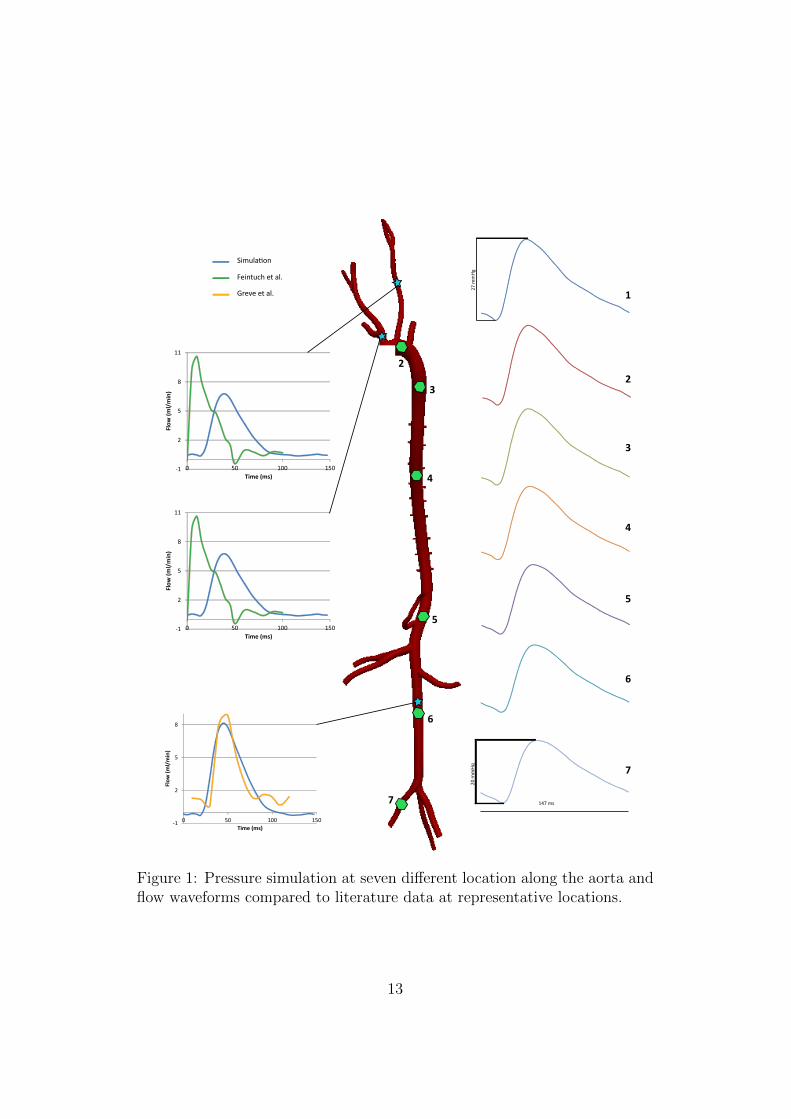
• An inflow boundary Γg. In this face of the model a flow wave form is

prescribed.

• A vessel wall boundary Γs. This boundary represents the interface

between the fluid domain and the vessel wall. Different conditions are

23

applied depending on whether a rigid or deformable wall assumption is

considered.

• An outflow boundary Γh. A weak pressure obtained via coupling with

a RCR lumped parameters condition is used in order to represent the

distal vasculature.

Figure 1.2: Tipical boundaries of a fluid domain in hemodynamics

To set up the fluid dynamic simulation, precise information on mice hemo-

dynamics and geometry is necessary; this information should be preferentially

measured in vivo. The small dimensions and fast heart rate (∼600 bpm) com-

plicate the acquisition of necessary data and this lack of knowledge makes

harder the validation of the model.

In the interest of investigating pressure waveforms and their role in arte-

rial stiffening is important to capture pulse pressure propagation. For this

purpose, it is mandatory to account for the deformability of the wall vessel

using fluid structure interaction (FSI) techniques. FSI methods have been

applied to patient-specific models of the thoracic aorta; where good agree-

ment between simulated and observed vessel motion and hemodynamics was

obtained [23]. However simulation of pulse wave velocity and pressure prop-

agation has not been validated in a mouse model yet.

24

1.3.1 Outflow boundary conditions

Outflow boundary conditions are a critical component of the mathematical

model. The choice of outflow boundary conditions was a significant influence

in 3-D simulations of blood flow, as they represent the peripheral vasculature

which strongly affects velocity and pressure fields in the 3-D domain.

In numerous fluid dynamic computations, prescribed velocity or pressure

outflow boundary conditions have been considered [24], [13]. This approach,

however, is inappropriate to model wave propagation phenomena. A slightly

more sophisticated approach for boundary condition specification is the con-

cept of resistance (R =P

Q). This boundary condition does not require the

specification of either flow or pressure at the outlet. However this approach

strongly affects wave propagation phenomena as it forces flow and pressure

waves to be in phase and it produces non physiologic pressures in the case

of flow reversal [25]. In this work a coupled 3D-0D approach presented in

Figueroa et al. [16] and Vignon-Clementel [26] has been used. Lumped pa-

rameter models are coupled to the 3-D equations of blood flow and vessel

wall dynamics. In these models, the parameters are assumed to be uniform

in each spatial compartment and their behavior is described by a set of or-

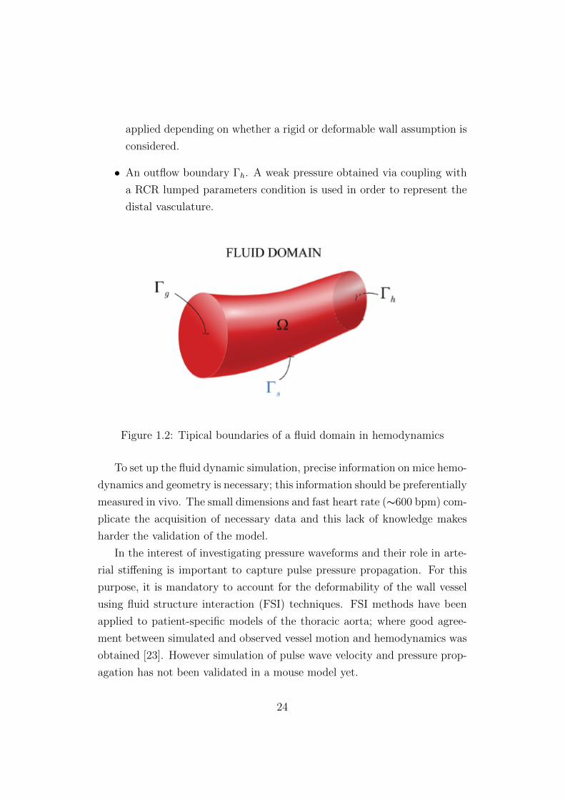
dinary differential equations. The specific lumped parameter model used is

a 3 element Windkessel model composed by a proximal resistance connected

in series with a parallel of distal resistance and compliance (see Figure 1.3).

An explicit relationship of pressure as a function of flow rate or velocity can

be derived at the coupling interface.

The use of Windkessl models as outflow boundary condition in complex

models with large number of vessels requires the specification of numerous

parameters. In this work a systematic approach to obtain these RCR param-

eters based on 1D-theory is considered [15].

There have been a few computational simulations of hemodynamics in

mice models. Huo et al. [24] investigated the distribution of hemodynamic

parameters in the mouse aorta and primary branches. They prescribed pres-

sure outflow boundary conditions (i.e, no reduced-order lumped parameter

model). Simplifications were made for the vessel geometry (assumed cylin-

25

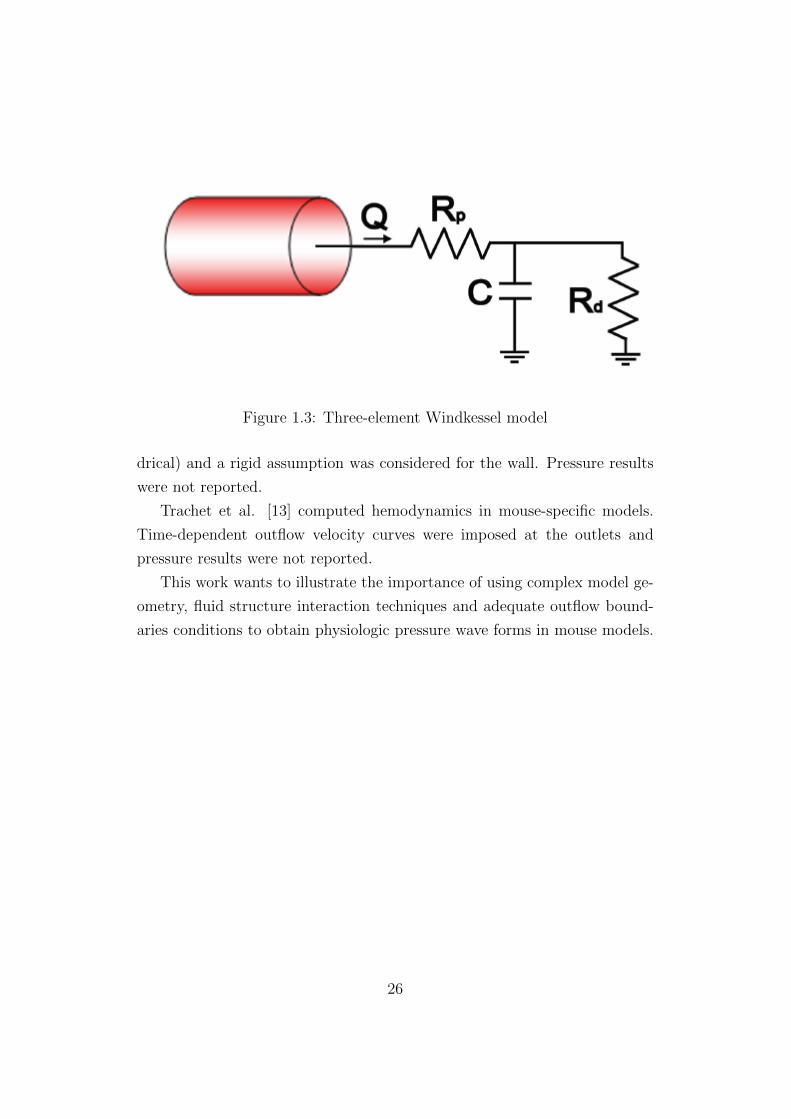
Figure 1.3: Three-element Windkessel model

drical) and a rigid assumption was considered for the wall. Pressure results

were not reported.

Trachet et al. [13] computed hemodynamics in mouse-specific models.

Time-dependent outflow velocity curves were imposed at the outlets and

pressure results were not reported.

This work wants to illustrate the importance of using complex model ge-

ometry, fluid structure interaction techniques and adequate outflow bound-

aries conditions to obtain physiologic pressure wave forms in mouse models.

26

Chapter 2

Methods

In this chapter, we provide an overview of the data available in the literature

on vascular geometry, flow and pressure, and mechanical properties. We then

describe the specific steps taken to produce one mouse-specific geometry.

We finish the chapter with a description the Computational Fluid Dynamics

framework used in this work.

2.1 Data research in literature

Hemodynamic, geometrical and mechanical mice data allow to set up the

computational simulations with adequate boundary conditions and to vali-

date the results against the in vivo measurements. The fast heart rate (in

the order of 600 beats/min) makes it difficult to use contrast agents for en-

hanced imaging in mouse. When building a geometric model of the mouse

vasculature, it is important to pay attention to weight, age and strain of the

mice tested, since the results are strongly depending on these factors.

2.1.1 Flow data

Reliable in vivo flow waveform measurements are important both for ade-

quate inflow boundary condition at the level of ascending aorta, and also

to validate the results. Lujan et al. [2] describe for the first time the

use of an intact, conscious, and unrestrained mouse model of myocardial

27

ischemia/reperfusion and infarction. A 1.6-mm Silastic-type Doppler ultra-

sonic flow probe was permanently implanted on the ascending aorta and an

occluder on the coronary artery. Measurements of ascending aortic blood

flow were recorded in conscious mice, at rest and during exercise, before and

during coronary artery occlusion, reperfusion and infarction. This model

provides data free of the influence of anaesthetics, surgical trauma and re-

straint stress. The procedures were done in 16 male C57BL/6 mice 3 to

4 months of age with body weight 25-30g. The measurements were taken

ten days after surgery. The paper reports the plot of ascending aorta flow

recorded in control mice for six cardiac cycles together with the ECG tracing

(see Figure 2.1). Since the recorded flow signal is not periodic; an average

signal was calculated to use in the simulation. The ECG peaks were used

to determine the starting point of each cycle. Each cycle was normalized in

time and amplitude. This operation lead to a flow waveform with a Qmean

of 11.92 ml/min (see Figure 2.2).

Feintuch et al. [3] studied hemodynamics in the mouse aorta using a

combination of Doppler ultrasound, MRI measurements, and numerical mod-

elling. Eight inbred C57BL/6 adult mice were studied with Doppler ultra-

sound imaging: 4 males and 4 females, 20–25 g body weight. The animals

were anesthetized with 1.5% isoflurane through a face mask. Blood flow ve-

locity was measured at the mid level of the ascending aorta and proximal

innominate artery, left common carotid artery, and left subclavian artery.

Blood flow patterns were also measured using MRI in five inbred C57BL/6

mice: 3 males and 2 females, 20–25 g body mass. The mice were anesthetized

for the scan duration with a mixture of 1.6% isoflurane gas and oxygen. Flow

data was recorded in the ascending aorta, innominate artery and left carotid

(see Figure 2.3). The measurements revealed a difference in total blood vol-

ume obtained with Doppler ultrasound and MRI. The Doppler ultrasound

tends to overestimate the flow because it measures blood velocity in the cen-

tre of the vessel, which is multiplied by the vessel cross-sectional area to get

flow. Since the ascending aortic flow is comparable to that reported by Lujan

article, innominate artery and left carotid flow data will be used to validate

the flow output obtained by the simulations.

28

Figure 2.1: Flow waveform in ascending aorta reported in Lujan t al. [2]

29

Figure 2.2: Average inflow signal obtaine from the Lujan data.

Lastly Greve et al. [4] measured blood flow in the infra-renal abdominal

aorta using phase-contrast magnetic resonance imaging at 4.7 tesla in five

male C57BL/6 mice, from 8 to 12 weeks old. During imaging, animals were

anesthetized with isoflurane and the body temperature was maintained at

37C using warm air. Infra-renal abdominal aortic flow was reported (see

Figure 2.4).

2.1.2 Pressure data

There are two general methods to measure blood pressure in mice: non-

invasive and invasive. The tail-cuff technique is the most used as non-invasive

methodology and it has the following advantages:

• It allows repeated measurements without introducing alterations in the

physiology of the animal;

• It correlates well with mean aortic pressure measured by others meth-

ods such fluid-filled catheters;

• It permits blood pressure measurements over long periods of time;

30

Figure 2.3: Flow data in innominate artery and left common carotid cal-culated from high-resolution magnetic resonance reported in Feintuch et al.Feintuch et al. [3]

31

Figure 2.4: Flow data in the infra-renal abdominal aorta, Greve et al. [4]

32

• It makes it possible to test a large number of subjects quickly;

• It is relatively inexpensive.

The disadvantages that can restrict its use are:

• It necessitates constraint and warming of the mouse: these procedures

produce stress and therefore alteration of the blood pressure;

• It shows variable results due to movement artifacts. A good matching

between tail-cuff and arterial pressure is only obtained when the subject

is at rest;

• It compares better with mean arterial pressure than with systolic pres-

sure measured with invasive methods;

• The mouse need anaesthesia and this can lower the pressure readings.

Blood Pressure measurements using a tail-cuff system have been collected

in a number of different inbred strains of mice and made available at the MPD

web site: http://phenome.jax.org.

Tsukahara et al. [27] measured diastolic and systolic pressure in 15 inbred

mouse strains using tail cuff. The mice were 10 weeks old. In order to collect

reliable data, the mice were conditioned to blood pressure measurement and

an average of 100 pressure readings in each mouse (20 measurements in 5

consecutive days) were performed. The pulse wave was recorded with a sen-

sor (BP-98A) attached to the tail cuff. For C57BL/6J strain mice a diastolic

pressure of 73.2 mmHg and a systolic pressure of 114.6 mmHg were reported.

Invasive methods allow direct measurements of arterial pressure using

indwelling fluid-filled catheters, radiotelemetry systems or transducer-tipped

catheters. The implantable catheter is set into an artery and it is associated

to a pressure transducer. Some of the advantages of this technique include:

• Consistent and reproducible measurements;

• Calibration is both simple and accurate;

33

• Measurements over long period of time can be acquired with low stress.

Disadvantages of indwelling catheters are:

• Surgery and the use of anesthesia may cause changes in blood pressure

and heart rate;

• Possible catheter occlusion;

• Potential surgical contamination;

• Limited dynamic feedback: this can affect the recording of systolic and

diastolic pressures;

• Specialized surgical skills are needed.

Reddy et al. [5] evaluated the pressure in the left iliac artery using a fluid

filled catheter. Five wild type mice, with an averaged body weight of 24±2g

were tested. The animals were anesthetized with continuous flow of isoflurane

and oxygen. The values reported in Table 2.1 for systolic, diastolic and mean

pressure were obtained for the iliac artery.

Systolic pressure 99± 15Diastolic pressure 65± 11

Mean pressure 80± 12

Table 2.1: Iliac artery pressure measurements, Reddy et al. [5].

In a different study, Redyy et al. [6] determined input aortic impedance

in adult and old mice. The mice tested were B6D2F1 type, 8 mice were 8

months old (adult) and 9 mice were 29 months old (old). The blood pressure

in the ascending aorta was measured by a pressure catheter of 0.36 mm diam-

eter, PressureWire3, RADI Medical System, Uppsala, Sweden. The catheter

was positioned as close as possible to the aortic root. During the surgery

the mice were anesthetized with a continuous flow of isoflurane and oxygen.

Table 2.2 summerizes the experimental results.

34

Adult mice Old miceBody weight, g 35.6± 0.2 34.6± 0.7

Heart rate, beat/min 406± 26 386± 32Mean aortic pressure, mmHg 73± 7.7 92± 4.0

Systolic pressure, mmHg 88± 8.8 116± 4.5Diastolic pressure, mmHg 59± 7.0 73± 3.9

Pulse pressure, mmHg 29± 4.9 42± 2.2

Table 2.2: Pressures in the aortic root measured through implantablecatheter Reddy et al. [6].

Radiotelemetry systems for recording blood pressure consist of a blood

pressure sensor and a transmitter. It is possible to acquire long-term mea-

surements of unrestraint mice. This system is becoming the gold standard

for blood pressure recordings in conscious mice. The advantages compared

to other techniques are:

• It is possible to obtain pressure measurements in awake mice without

restraints;

• Continuous recordings are possible;

• High-fidelity data;

• Long-term catheter patency;

On the other hand, it requires significant microsurgical technique skills.

Van Vliet et al. [7] used blood pressure telemeter to characterize 24h

pressure in mouse lacking the gene for endothelial nitric oxide synthase and

the corresponding control strain, C57BL/6J. Measurements were analyzed

for the entire 24h period, and the two 12-hours periods of light and darkness.

The control mice had an average weight of 27.3 ± 0.4g. At 9-12 weeks the

animals were put in individual cages and 2 weeks later the telemeter was

implanted and turned on on the 10th day. The tip of the telemeter was

inserted into the aortic arch via the left carotid artery; the telemeter body

was allocated subcutaneously on the right flank. During the procedure, the

mice were under ketamine and xylazine anaesthesia. Table 2.3 shows the

summary of the measurements.

35

24h Light period Dark periodMean aortic pressure, mmHg 104± 2 97± 1 110± 3

Systolic pressure, mmHg 119± 2 112± 2 125± 3Diastolic pressure, mmHg 87± 2 81± 2 94± 2

Pulse pressure, mmHg 31.6± 1.5 31.5± 1.5 31.7± 1.5Heart rate, beat/min 596± 6 556± 7 625± 9

Table 2.3: Blood pressure in the aortic arch measured through radio teleme-try systems, Van Vliet et al. [7]

McGuire et al. [8] used radiotelemetry system to measure pressure in

conscious unrestrained mice. As control mice they used 33 male C57BL/6J,

from 10-20 weeks of age and 25-30g of weight. The room lighting was set

to 12 h light and 12 h darkness cycles. The telemeter (TA11PA-C10, Data-

sciences Inc.) was implanted via the right carotid artery. During the surgery

the animals were anesthetized with isoflurane and 13-18 days were allowed

for the mice to recover. The pressure data were then recorded continuously

for 3-9 days at baseline. Table 2.4 summarizes the findings of the experi-

ments.

12h light 12h darkSystolic pressure, mmHg 118± 1 131± 1Diastolic pressure, mmHg 89± 1 101± 1

Pulse pressure, mmHg 29± 1 31± 1Heart rate, beat/min 587± 4 607± 6

Table 2.4: Blood pressure in the aortic arch measured through radio teleme-try systems, McGuire et al. [8]

Lastly transducer-tipped catheters procure high-fidelity pressure record-

ings. Since measurements are taken directly at the source and are usually

not affected by movement artifacts. The most used catheter is the 1.4-Fr

Millar Mikro-Tip pressure transducer. This device is able to capture signals

at high frequencies as the pressure changes during systole in mice. Due to

the catheter stiffness, it is necessary to anesthetize or sedate the mice during

the procedure. The calibration of the instrument tends to drift with time,

36

therefore the use of such catheters is limited to short-time recording.

Lorenz and Kranias [28] used a Millar Mikro-Tip transducer to measure

pressure in the ascending aorta. Seven wild type C57B1/6 mice with an

average body weight of 31g were tested. The catheter was positioned in

the ascending aorta at the level of the right carotid artery. The mice were

anesthetized with ketamine and thiobutabarbital during the surgical proce-

dure. After the surgery the animal were allowed to stabilize for 30-45min. A

mean average pressure of 72 mmHg and a systolic pressure of 97 mmHg are

reported as baseline values for the wild type mice.

After careful consideration of the advantages and disadvantages of the

different pressure recording techniques, the data reported by Van Vliet et al.

[7] was chosen as gold standard in this work.

2.1.3 Geometrical data

Currently the most used technique to study the arterial geometry in mice

is the vascular corrosion casting. It consists of the injection of a hardening

resin in the vascular system of the animal to obtain a plastic cast that can

be scanned. This technique allows to overcome the problems faced during

traditional MRI of mice, since the high heart rate makes the use of contrast

agents difficult. A downside of this technique is the euthanasia of the ani-

mal and therefore the inability to perform other tests on the same subject.

Furthermore the reliability of the data acquired is often times questionable

since the diameters can be affected by factors such as vessel tone, perfusion

pressure and shrinkage of the resin used.

Vandeghinste et al. [9] investigated the differences between in vivo micro-

computed tomography (CT) and the micro-CT scanning of a vascular corro-

sion cast. They used a new contrast agent specially developed for cardiovas-

cular imaging in mice: Fenestra VC-131. Nine wild-type mice were tested,

with body weights ranging from 14 to 35g and ages raging from 5 to 27 weeks

old. The mice were first anesthetized, then scanned in vivo and one week

later the casting was performed on the same animals. High-quality casts were

obtained and used for four animals. The authors compared the diameters

37

of the vessels, the bifurcation angles and the wall shear stress levels in CFD

simulations.

Cast(mm) In vivo(mm) Difference(%)Ascending aorta 1.08± 0.09 1.43± 0.07 34.21

Brachiocephalic trunk 0.55± 0.06 0.78± 0.05 41.82Aortic arch 0.93± 0.05 1.24± 0.07 33.33

Common carotid artery 0.4± 0.07 0.51± 0.01 27.50Subclavian artery 0.45± 0.05 0.62± 0.04 37.78Descending aorta 0.87± 0.09 1.13± 0.09 29.89

Table 2.5: Comparison of diameters obtained with casting and in vivo micro-CT, Vandeghinste et al. [9]

The results (see table 2.5) show a significant difference (30%) in vessel

diameter estimated by the two methods. The cast solution was injected with-

out control on the pressure and therefore the perfusion pressure was likely

too low. The authors hypothesized that 10% to 20% of the observed dif-

ference can be related to the large volume of contrast agent injected in the

subject during the in vivo scans. This extra volume could be responsible of

augmented arterial pressure in vivo. Furthermore, as no cardiac gating was

applied during the study it was not possible to determine diastolic dimen-

sions. The authors hypothesize that the in vivo diameters are close to systolic

values whereas the in vitro (casting) diameters are more representative of the

diastolic state.

Casteleyn et al. [10] also analyzed the mice vascular anatomy through

vascular corrosion casts. Thirty female mice, 2 months old in age with a

mean weight of 30.6 g were tested. The purpose of that work was to describe

the anatomy and geometry of the murine heart and thoracic aorta including

its main branches. After sacrificing the animals, the abdominal aorta was

catheterized with a 26 gauge catheter and Batson’s #17 solution was gently

injected free-hand in the retrograde direction. Table 2.6 contains the sum-

mary of the results. This study has once again no perfusion pressure control

and diameters are even smaller than those reported by Vandeghinste et al.

[9].

Hinton et al. [11] investigated the valve structure in different phases

38

Diameter(mm)Ascending aorta 0.82± 0.01

Aortic Arch 1.06± 0.02Descending aorta 0.74± 0.02

Brachiocephalic trunk 0.54± 0.02Left common carotid 0.35± 0.02

Left subclavian 0.38± 0.02

Table 2.6: Vessel diameter measurements obtained by Casteleyn et al. [10]

of mouse life. The mice studied were wild-type mixed-sex C57BL6 obtained

from Jackson Laboratories (Bar Harbour, ME). The life phases studied were:

• New born: 10 days

• Juvenile: 1 months

• Young adult: 2 months

• Old adult: 9 months

• Aged adult: 16 months

The body weight was measured at every step since geometric dimensions

can highly vary depending on age or size. Cross-sectional, two-dimensional

Doppler transthoracic echocardiography was performed by experienced sono-

graphers using a Visual Sonics Vevo 770 Imaging System (Toronto, Canada).

Mice were anesthetized with 1% to 2% isoflurane. All the reported data were

averaged from three repeated measurements (see Table 2.7).

Aortic root(mm) Ascending aorta(mm) Body weight(g)10 days 0.8 0.88 7.2± 0.91 month 1.05 1.18 11.2± 1.02 month 1.23 1.39 17.3± 1.49 month 1.35 1.52 33.0± 6.016 month 1.15 1.36 26.4± 4.0

Table 2.7: Aortic root and ascending aorta diameters, Hinton et al. [11]

Wan et al. [12] studied increases in arterial stiffness in the common carotid

artery using genetically-modified mouse models lacking fibulin-5, a critical

39

protein for the functionality of elastin fibers. Biaxial biomechanics test and

multiphoton microscopy imaging were performed on isolated carotid arteries

of seven fbln5+/+ and fbln5-/- adult C57BL/6 mice, 13 weeks old and 28.93

g body weight. The carotid were collected, dissected and put on the glass

cannulae of the biomechanical testing device. Pressure-diameter data were

collected from 0 to 180 mmHg at constant axial extensions. The P-d test

were executed at different stretches, here the measurements collected at in

vivo stretch and 100mmHg pressure are reported (see table 2.8).

In vivo dimensions(mm)Inner diameter 0.603Outer diameter 0.652Wall thickness 0.024

Table 2.8: Carotid diameters obtained via biaxial tissue testing by Wan etal. [12]

Trachet et al. [13] used micro-CT scans to investigate the anatomy of

the abdominal aorta and its main branches in mice. They also utilized high-

frequency ultrasound imaging to acquire flow information in each branch.

Ten C57BL/6 ApoE-/- mice, 12 ± 3 weeks old, were studied. An osmotic

pump was implanted to continuously infuse Angiotensin II, to induce the

development of an abdominal aneurysm. Measurements were taken before

pump implantation and after 31 days. To perform the micro-CT, the mice

were anesthetized with 1.5% isoflurane and 100 microliter/25g of Aurovist

was injected intravenously. See Table 2.9 for results.

BW,g HR,bpm PAA CEL MES RREN LREN DAA24.4 444 1.24 0.43 0.65 0.54 0.43 0.73

Table 2.9: Mean diameters reported by Trachet et al. [13]. BW: body weight,HR: heart rate, PAA: proximal abdominal aorta, CEL : celiac artery, MES:mesenteric artery, RREN: right renal artery, LREN: left renal artery, DAA:distal abdominal artery. The diameters are reported in mm.

A summary of the data used in this work is reported in the table 2.10.

The age and the size of the animals tested have been taken into account in

the choice, since they strongly affect the geometrical dimension.

40

LOC Originalcastingdiameter

Literaturediameter

Description of methodol-ogy

AAo 0.9153 1.43 Vandeghinste (2011) [9];in vivo micro-CT. The di-ameter is calculated asmean of a large area.

AA 0.8347 1.24 Vandeghinste (2011) [9];in vivo CT. The diameteris calculated as mean of alarge area.

DA 0.6842 1.13 Vandeghinste (2011) [9];in vivo micro-CT. The di-ameter is calculated asmean of a large area.

IN 0.4573 0.78 Vandeghinste (2011) [9];in vivo micro-CT. The di-ameter is calculated asmean of a large area.

LCC 0.2701 0.51 Vandeghinste (2011) [9];in vivo micro-CT. The di-ameter is calculated asmean of a large area.

LSUB 0.2989 0.62 Vandeghinste (2011) [9];in vivo micro-CT. The di-ameter is calculated asmean of a large area.

CEL 0.2756 0.43 Trachet (2011)[13]; micro-CT scans.

MES 0.2985 0.65 Trachet (2011)[13]; micro-CT scans.

RREN 0.30 0.54 Trachet (2011)[13]; micro-CT scans.

LREN 0.2309 0.43 Trachet (2011)[13]; micro-CT scans.

Table 2.10: The location, the diameter of the model and the diameter of thebest reference are reported. AAo: ascending aorta, AA: aortic arch, DA:descending aorta, IN: innominate artery, LCC: left common carotid, LSUB:left subclavian, CEL: celiac artery, MES: mesenteric artery, RREN: rightrenal artery, LREN: left renal artery. Measurements reported in mm.

41

2.2 Building the 3D geometric mouse model

2.2.1 Original geometry

A 3-D model of the mouse arterial geometry was built using the custom soft-

ware Simvascular; using micro-CT imaging of a vascular casting of a,27.14

weeks old, 42.64 g, mouse. The vascular corrosion casting and the corre-

sponding geometric model were obtained at the Department of Biomedical

Engineering of Yale University, New Haven, CT, USA.

Briefly, the mouse was anesthetized using sodium pentobarbital, the left

ventricle was cannulated at its apex using with a 25-G needle and the ma-

jor distal vessels (subclavians, carotids, renals and iliacs) were ligated. The

aorta was then flushed with heparinized saline (110 U/Kg). This precast-

ing treatment is necessary in order to completely remove the blood from the

target vessel. The goal is then to fill the entire vascular bed and to obtain

endothelial cell imprints on the surface of the cast [29]. The aortic tree was

perfused at a fixed pressure of 100mmHg for 2 hours with 4% paraformalde-

hyde follwed by injection of Batson’s no. 17 Plastic replica Kit (Polysciences,

WA) for 2.5 hours using the manufacturers specifications. It is critical to ad-

just the injection pressure in order to fill the vascular bed completely. The

plastic cast was then gently excised and placed in a KOH solution to remove

adherent tissue. The geometry of the aortic tree was then imaged using

micro-CT.

SimVascular allows users to generate geometric models from imaging

data. During the segmentation procedure, the arterial lumen boundary is

defined using a combination of manual demarcation, image thresholding, and

level-set segmentation [30]. To perform the segmentation a set of vessel cen-

terline paths are created and then 2-D segmentations are built along each

path (see Figure 2.5). A 3-D geometric solid model is created by lofting the

2-D segmentations with Non-Uniform Rational B-Splines (NURBS).

The mouse vasculature model includes the ascending, descending, and

abdominal aorta and significant segments of the subclavians, the carotids,

the renal arteries, mesenteric, celiac, and tail; see Figure 2.6.

42

Figure 2.5: Path along the aorta and 2-D segmentations of the vessel lumen.

2.2.2 Up-scaled model

In the casting process, the injection pressure was insufficient and conse-

quently the vessel diameters were too small relative to the reference values

given in Table 2.10.

Understimation of the vessel caliber has a very negative impact on the

computed hemodynamics. When a physiological flow waveform is pushed

through the under-represented geometry, the resulting pulse pressure is much

higher than what is observed physiologically. This is of course due to the ar-

tificially high resistance of the narrower than normal vessels. Furthermore,

these big resistances makes it difficult to choose boundary condition param-

eters required to obtain the desired flow splits. We have therefore modified

the vessel diameters to match the literature data presented earlier. For each

segmentation, a centroid and mean radius were calculated. The mean radius

for each vessel was then scaled up to match the dimensions reported in Table

2.10. A different scaling factor was used for each segmentation. The aorta

was upscaled using three reference diameters: the ascending aorta, the aortic

43

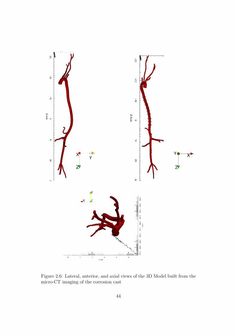
Figure 2.6: Lateral, anterior, and axial views of the 3D Model built from themicro-CT imaging of the corrosion cast

44

arch and the descending aorta such that each reference radius is the mean of

the radii in a given section of the vessel. For those vessels for which a refer-

ence diameter was not available, the scale factor of the closest segmentation

was used to scale all segmentations in that vessel (see Figure 2.7 ).

Figure 2.7: View of the original geometry (inner) and the upscaled geometry(external overlay).

45

2.2.3 Intercostal arteries

The image data did not allow for visualization of the intercostal arteries,

which take up a blood flow up to 17.3% of the mouse cardiac output [? ]. In

the interest of making the pressure gradient across the thoracic aorta and the

flow distributions more realistic, intercostal arteries were added to the model

using reference diameters and branch distances [14]. For each of the nine

pairs of intercostal arteries, the branch distance was defined as the relative

length along the aorta path spline (see Table 2.11). The branch origin was

calculated using the mean of the centers of the two nearest aorta segmen-

tations, weighted by the relative distance to each segment. The intercostal

paths were defined as straight lines parallel to the branching angle of the cor-

responding renal artery, perpendicular to the aorta path, and with a length

of twice the aorta diameter at that point.

Fractional longitudinal position Location down the aorta0 Aortic semilunar valve

0.20± 0.013 First pair of intercostal arteries0.24± 0.014 Second pair of intercostal arteries0.29± 0.0066 Third pair of intercostal arteries0.34± 0.0087 Fourth pair of intercostal arteries0.38± 0.0080 Fifth pair of intercostal arteries0.42± 0.0064 Sixth pair of intercostal arteries0.47± 0.0087 Seventh pair of intercostal arteries0.51± 0.0096 Eighth pair of intercostal arteries0.55± 0.012 Ninth pair of intercostal arteries

1 Common iliac artery

Table 2.11: Fractional longitudinal position of the intercostals on branchvessel along the aorta, Guo et al. [14]

46

2.3 Computational fluid dynamics method

2.3.1 Mesh and mesh adaptivity

Good quality computational grids are needed to ensure a proper numerical

simulation. An initial mesh was generated using the meshing libraries in

Simvascular. A global value for the element size of 0.08 mm was used together

with a refinement on the intercostal arteries. Boundary layer meshing was

also used in order to ensure good density of elements close to the vessel wall,

where all the action happens. With these parameters a 2 million element

mesh was obtained.

This mesh was used to run a rigid simulation for 2 cardiac cycles using

1470 time steps per cycle (Tcycle = 0.147s). The results of this first simulation

were used to adapt the mesh taking into account the distribution of velocity

gradients in the arterial network. The adaptation mesh algorithm reduces

the number of elements in regions of low velocity gradients and increases the

number of elements in areas of large velocity gradients. The objective of this

”a-posteriori” error estimation-based mesh adaptivity technique is to obtain

a uniform distribution of error in all spatial directions. This mesh adaptation

operation reduced the number of elements in the initial mesh to less than

1 million (see Figure 2.8). This reduction of number of elements allows to

decrease prominently the time to complete the same simulation to one third

of the time required to solve the same problem on the initial mesh.

2.3.2 Multiscale modelling approach

The 3-D equations representing the flow of an incompressible Newtonian

fluid are the so-called Navier-Stokes equations of motion and mass continuity,

together with adequate initial and boundary conditions. The weak form is

reported:

47

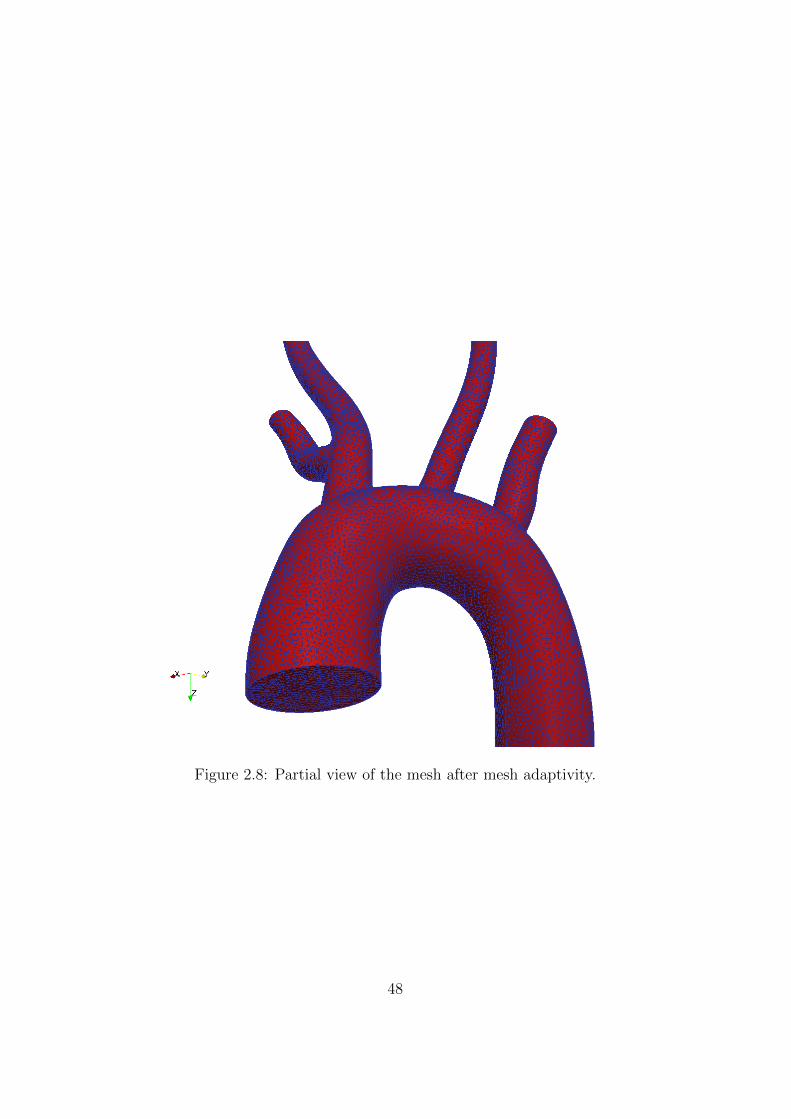
Figure 2.8: Partial view of the mesh after mesh adaptivity.

48

∫Ω

w · (ρv,t + ρv · ∇v− f) +∇w : (−pI˜ + τ˜)dx (2.1)

−∫

Ω

∇q · vdx−∫

Γout

w · (−pI˜ + τ˜) · nds+

∫Γ

qv · nds

where v and p are the fluid velocity and pressure, f is a body force, w and

q are weighting functions, and ρ is the blood density. Ω is the fluid domain,

whose boundary Γ is split into a Dirichlet partition Γin, Neumann partitions

Γout and Γt such that Γ = ∂Ω = Γin ∪ Γout ∪ Γt and Γin ∩ Γout ∩ Γt = ∅.A coupled multi-domain method is used [31] in order to represent the

entire arterial vasculature from the central aorta to the capillaries. This

method employs a decomposition of the spatial domain Ω into an upstream

”numerical” domain Ω, and a downstream ”analytical” domain Ω′ such that

Ω∩Ω′ = ∅ and Ω ∪ Ω′ = Ω (see Figure 2.9). These two domains are separated

by the interface Γout. A similar decomposition is applied to the variables fluid

velocity v = (vx, vy, vz) and pressure p. The solution vector V = v, pT is

separated into a component defined within the numerical domain Ω and a

component defined within the analytical domain Ω′:

V = V + V’ with V|Ω′ = 0 and V′|Ω = 0

This decomposition satisfies the condition V = V′ at the interface Γout, and

is also applied to the weighting functions. This decomposition will allow

different degrees of solution resolution in the two domains. Ω represents

the 3-D domain in which the Navier-Stokes equations for an incompressible

Newtonian fluid are solved. Ω′ corresponds to the distal vascular network

and microcirculation where the flow physics are described using a lumped-

parameter formulation.

The coupled-multidomain method produces a variational form for the

numerical domain similar to the one given by the Eq. 2.1, where the integral

term defined on Γout is written in terms of operators M = Mm,MCT |Γout

and H = Hm, HCT |Γout

49

∫Ω

w · (ρv,t + ρv · ∇v− f) +∇w : (−pI˜ + τ˜)dx (2.2)

−∫

Γout

w · (M˜m(v, p) +H˜m) · nds−∫

Ω

∇q · vdx +

∫Γ

qv · nds

+

∫Γout

q(MC(v, p) + HC) · nds = 0

where subscripts m and c denote the fluid momentum and mass balance

components of the operators, respectively. These operators are defined in the

domain Ω′ based on the model chosen to represent blood flow and pressure

in the distal analytical domain.

In this work a three-component Windkessel model has been adopted: this

requires the definition of a proximal resistance Rp, compliance C and distal

resistance Rd. These three parameters are used to define the operators M

and H [26].

Figure 2.9: The overall fluid domain Ω is separated into an upstream numer-ical domain Ω and a downstream analytical domain Ω′, demarcated by theinterface Γout.

50

2.3.3 Fluid-structure interaction

The majority of computational fluid dynamics simulation in mice [3] [13]

[24] have assumed rigid arterial walls, which disallows accurate calculations

of blood pressure despite possibly achieving good estimates of velocity field.

We are interested in pulse pressure estimation and pulse wave velocity which

are fundamental to study the relationship between arterial stiffening and

hypertension. In order to capture pulse pressure propagation is mandatory

to use fluid structure interaction (FSI). Effectively, wave propagation phe-

nomena in the cardiovascular system can only be described considering wall

deformability since blood is described as an incompressible fluid. In this work

the FSI ”Coupled Momentum” method developed by Figueroa and Taylor at

Stanford, was used. The method starts from the conventional stabilized finite

element formulation for the Navier-Stokes equations in a rigid domain (see

Eq. 2.1) (Figueroa et al. [16]). The method then incorporates the elastody-

namic equations representing the deformation of the wall over a cardiac cycle

as a boundary condition for the fluid domain. The degrees-of-freedom of the

fluid and the solid domains are strongly coupled. The effect of the vessel

wall boundary is added in a monolithic way to the fluid equations. It em-

ploys a linearized stiffness and membrane model for the vessel wall resulting

in a robust scheme with minimal computational cost beyond that required

for rigid wall problems. The zero-velocity Dirichlet condition prescribed on

the lateral boundary in rigid wall formulations is replaced by a Neumann

condition which is the traction originating from interactions with the vessel

wall. The weak form of the governing equations for the fluid domain can be

written as:∫Ω

w · (ρv,t + ρv · ∇v− f) +∇w : (−pI˜ + τ˜)−∇q · vdx (2.3)

+

∫Γout

−w · t + qvnds+

∫Γin

qvnds

+h

∫Γt

−w · ρsv,t +∇w : σ˜(u)ds− h∫∂Γout

w · tsdl +

∫Γt

qvnds.

Where h is the arterial thickness, ρs the density of the arterial wall, t is

51

a traction boundary condition four the fluid outflow face and ts is a trac-

tion boundary condition for the wall on the outlet. Using a deformable wall

model, an accurate description of the constitutive behavior of the tissue is

necessary. The arterial wall is modeled as a thin, incompressible, homoge-

nous, isotropic, linear elastic membrane characterized by an elastic modulus

E, a Poisson ratio ν = 0.5 and a thickness h. It is necessary to characterize

structural stiffness of the vessel, hence the young modulus E and the wall

thickness h. The local thickness h was defined as 10% of the local radius

r [1]. Biaxial stiffness values in four different locations were experimentally

obtained in the Department of Biomedical Engineering of Yale University.

Linearized stiffness values at in vivo axial stretch and pressure of 100mmHg

were measured for ascending, descending and abdominal aorta, as well as

right common carotid artery. The stiffness matrixes are reported in Figure

2.10. In this work, we used the calculated circumferential stiffness as a sur-

rogate of isotropic stiffness, since it is the component that mostly affects

radial deformation. In future work, we will consider the full biaxial stiffness.

The three aortic measurements were interpolated to define stiffness values

for each element of the mesh along the aorta. The value of the left common

carotid was used for upper and lower branches (see Figure 2.11). In order to

study the effects of increased stiffness on the hemodynamics, the structural

stiffness of the wall was also increased to represent age-related changes. Two

additional simulations were run by scaling the young modulus E by a factor

of 2 and 3, respectively.

2.3.4 Tissue support

Another important aspect to take into account in the FSI simulation is the

support exerted by the perivascular tissue and other organs on the arterial

wall. This tissue support helps to prevent non physiological oscillations in the

movement of arterial wall. A simple traction is applied on the outer bound-

ary of the vessel wall to represent the mechanical behavior of the perivascular

tissue [32]. This traction boundary condition consists of a viscoelastic term

with two parameters (a stiffness and a viscous parameter) that can be ad-

52

K =

1.987

0.767

0

0

0

0.767

1.758

0

0

0

0

0

1.066

0

0

0

0

0

0.312

0

0

0

0

0

0,287

Ascending aorta, λ=1.71

K =

3.145

0.610

0

0

0

0.610

1.232

0

0

0

0

0

0.804

0

0

0

0

0

0.195

0

0

0

0

0

0.191

K =

3.175

0.671

0

0

0

0.671

1.232

0

0

0

0

0

0.868

0

0

0

0

0

0.226

0

0

0

0

0

0.167

K =

2.727

0.917

0

0

0

0.917

1.279

0

0

0

0

0

1.090

0

0

0

0

0

0.201

0

0

0

0

0

0.147

Descending aorta, λ=1.50

Infra-renal abdominal aorta, λ=1.66 Right common carotid artery, λ=1.74

Figure 2.10: Biaxial stiffness values in four different location measured at invivo axial stretch λ and pressure=100mmHg.

justed to mimic the response of various physiological tissues.

2.4 Boundary condition specification

The three-element Windkessel model coupled at each outlet of the 3-D do-

main is an electrical circuit analogue of the circulation (0-D) composed of

a resistance R1 connected in series with a parallel of a resistance R2 and a

compliance C (see Figure 1.3). This model represents the small arteries and

arterioles, down to the capillary level. The pressure and the flow at each

Windkessel are related by the following ODE:

Q(1 +R1

R2

) + CR1∂Q

∂t=P − Pout

R2

+ C∂P

∂t(2.4)

where Pout is the pressure at the micro circulation (assumed to be zero here).

This Windkessel model prescribes a weak pressure on the outlet of the 3-

D domain for a given flow. For details on the specific implementation see

Vignon-Clementel et al. [26].

53

1230000.0

E [Pa]

1700000.0

1600000.0

1500000.0

1400000.0

1300000.0

1760000.0

0.00873

Thickness [mm]

0.1

0.1

0.0

0.0

0.0904

Figure 2.11: Tissue properties: young modulus interpolated from the dataacquired at Professor Humphrey’s lab and thickness defined as 10% of thelocal radius.

54

The parameters of the Windkessel model have been computed to reach

the target diastolic and systolic pressure Pd,Ps (see section 2.1.2). The initial

estimation of total resistance of the system is calculated as:

RT =Pm − Pout

Qmean

(2.5)

where Qmean is the mean inflow and Pm is the mean blood pressure, assumed

uniform throughout the arterial network. RT represents the total resistance

of the model (combination of the 3-D geometry and the distal Windkessel

model). We started off assuming that the resistance of the 3-D domain is

much smaller than the 0-D domain. The distribution of the total resistance

Rj = Rj1 + Rj

2 for each outlet j of the model has been derived using the

relationship

1

RT

=∑j

1

Rj⇒ RT

Rj=

Qj

Qmean

⇒ Rj = RTQmean

Qj(2.6)

For each outlet the proximal resistance Rj1 is assumed to be equal to the

characteristic impedance at the outlet of the upstream domain

Rj1 =

ρfcjd

Ajd

(2.7)

where cjd is the wave speed and Ajd the reference area at diastolic pressure.

This choice minimizes the amount of wave reflection at the outlet. The distal

resistance Rj2 for each outlet is then calculated as Rj

2 = Rj −R1.

The total compliance of the model CT is calculated using the approxima-

tion CT =dV

dP:

CT =Qmax −Qmin

Ps − Pd

∆t (2.8)

where Qmax and Qmin are the maximum and minimum inlet flow rates and

∆t is the difference between the time at Qmax and the time at Qmin.

The total compliance CT is then split between Cc (total compliance of

55

the 3-D model) and Cp (total peripheral compliance): CT = Cc + Cp.

Cc is the sum of the compliance of each vessel, which is calculated as

Cjc =

AjdL

j

ρf (cjd)2

(2.9)

where Lj is the length of the vessel j.

The total peripheral compliance is then calculated as Cp = CT −Cc. This

compliance is distributed among the different outlets in proportion to the

flow distribution.

Qj

Qmean

= (Rj

2

Rj1

)Cj

p

Cp

⇒ Cjp = Cp

Qj

Qmean

(Rj

1 +Rj2

Rj2

) (2.10)

Lastly, the wave speed cj at each outlet is estimated using two differ-

ent procedures, depending on the information available on the mechanical

properties.

• If stifness E and thickness h are known:

cj =

√βj

2ρAjd

(Ajd)

1/4; βj =4

3

√πEjhj (2.11)

• If stifness E and thickness h are not known (as in the case of rigid wall

analyses):

cj =a2

(2Rjd)

b2(2.12)

The value of cj is given in m/s. This is a non-dimensionally consistent

empirical formula [33]; where a2 = 13.3 and b2 = 0.3.

56

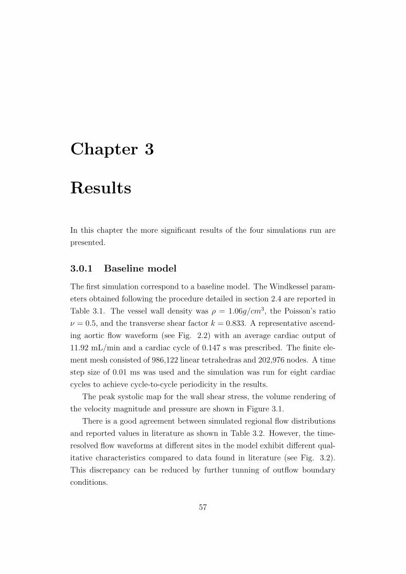
Chapter 3

Results

In this chapter the more significant results of the four simulations run are

presented.

3.0.1 Baseline model

The first simulation correspond to a baseline model. The Windkessel param-

eters obtained following the procedure detailed in section 2.4 are reported in

Table 3.1. The vessel wall density was ρ = 1.06g/cm3, the Poisson’s ratio

ν = 0.5, and the transverse shear factor k = 0.833. A representative ascend-

ing aortic flow waveform (see Fig. 2.2) with an average cardiac output of

11.92 mL/min and a cardiac cycle of 0.147 s was prescribed. The finite ele-

ment mesh consisted of 986,122 linear tetrahedras and 202,976 nodes. A time

step size of 0.01 ms was used and the simulation was run for eight cardiac

cycles to achieve cycle-to-cycle periodicity in the results.

The peak systolic map for the wall shear stress, the volume rendering of

the velocity magnitude and pressure are shown in Figure 3.1.

There is a good agreement between simulated regional flow distributions

and reported values in literature as shown in Table 3.2. However, the time-

resolved flow waveforms at different sites in the model exhibit different qual-

itative characteristics compared to data found in literature (see Fig. 3.2).

This discrepancy can be reduced by further tunning of outflow boundary

conditions.

57

Rp C Rd

Celiac 67.84 338.24 1479.07Intercostals 356.22 68.20 7334.46

Left ext. carotid 67.93 255.16 1616.13Left int. carotid 62.90 349.94 1178.41

Left iliac 26.79 719.08 877.94Left renal 44.99 555.17 901.12

Left subclavian 32.12 690.06 724.98Mesenteric 35.39 673.20 743.14

Right ext. carotid 143.85 219.65 2008.58Right int. carotid 39.78 468.33 942.03

Right iliac 39.77 560.49 1126.35Right renal 42.15 554.69 901.91

Right subclavian 55.54 444.62 992.28Tail 78.83 321.06 1966.32

Table 3.1: Windkessel parameters in the baseline simulation. The resistances

are expressed inPa · smm3

and the compliance in 10−6mm3

Pa.

Location %CO Simulation %CO ReferenceInnominate artery 17.09 17

Left common carotid 9.46 9.76Infra-renal aorta 17.06 17.1

Table 3.2: Simulated and reference values of %CO

58

Pressure [mmHg]120.0112.5105.00

Velocity [cm/s]6040201500

Wall shear stresses [dyn/cm ]1208040

2

Figure 3.1: Magnitude of the wall shear stress, volume rendering of thevelocity magnitude and pressure at the peak systolic.

59

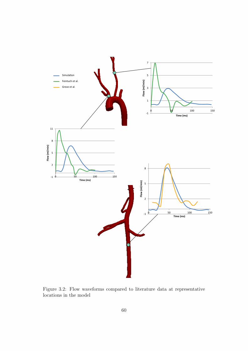
-1

1

3

5

7

0 50 100 150

Flow

(ml/

min

)

Time (ms)

-1

2

5

8

11

0 50 100 150

Flow

(ml/

min

)

Time (ms)

-1

2

5

8

0 50 100 150

Flow

(ml/

min

)

Time (ms)

Simulation

Feintuch et al.

Greve et al.

Figure 3.2: Flow waveforms compared to literature data at representativelocations in the model

60

Figure 3.3 shows pressure waveform at seven sites along the aorta. The

shape and pressure range of the waveform match data reported in literature

[34]. Indeed, the pressure rises in the systolic phase and then falls in an almost

exponential fashion. Pressure in the ascending aorta ranged from 93 to 120

mmHg. No increase in pulse pressure is observed down the aorta: all seven

locations exhibit similar amplification and contour. We therefore reproduced

reported literature data indicating lack of pressure pulse amplitude down the

aorta in mice [1].

3.0.2 Modified distal compliance case

Another simulation was run to investigate whether amplification of the pulse

is physiologically obtainable. We thus modified RCR values derived from

the 1-D theory (see Section 2.4) reducing the compliance of the distal vessel

(tail, iliacs, mesenteric, renals and celiac arteries) by a factor of 5.

Figure 3.4 shows how this change of RCR values leads to an augmentation

in pulse pressure along the aorta as desired: The proximal pulse pressure is

30 mmHg, while the distal pulse pressure is 34 mmHg.

3.0.3 Increased arterial stiffness

The impact of temporal changes in wall mechanical properties, due to aging

and hypertension, on pressure pulse propagation has also been investigated.

It is known that in mice, as in humans, aging increases aortic wall thickness

and collagen remodeling [17].Two additional simulations in which arterial

stiffness was increased to represent age-related changes in mechanical prop-

erties were performed. These two additional cases were obtained by scaling

the distribution of stiffness E of the baseline case by a factor of 2 and 3,

respectively. In these two cases the values of RCR were identical to the base-

line case, since the aging changes are observed to be largest in the aorta and

in central arteries. Figure 3.5 shows pressure waveforms at seven sites in the

aorta for all three cases.

61

12

3

4

5

6

7

1

2

3

4

5

6

7

27 m

mHg

147 ms

20 m

mH

g

Figure 3.3: Pressure waveform at different locations in the aorta.

62

Eh [P

a m

m]

1200

00.0

8000

0.0

4000

0.0

1600

00.0

1000

0.0

12

3 4

5809010

0

110

120

130

050

100

150

8090100

110

120

130

050

100

150

1: A

scen

ding

aor

ta2:

Aor

tic a

rch

3: D

esce

ndin

g ao

rta

4: S

upra

-ren

al a

orta

5: I

nfra

-ren

al a

orta

RCR

valu

es d

eriv

ed fr

om 1

-D th

eory

Redu

ced

com

plia

nce

in ta

il, il

iacs

, ren

als.

ce

liac

and

mes

ente

ric (5

x)

Figure 3.4: Pressure pulse propagation along the aorta for the baseline (left)and decreased peripheral compliance (right).

63

Eh [Pa mm]

400000.0

300000.0

200000.0

100000.0

12

3

4

5

6

7

Baseline case Ex2 Ex3

90

100

110

120

130

-10 10 30 50 70 90 110 130 150Time (ms)

90

100

110

120

130

-10 10 30 50 70 90 110 130 150

Pre

ssu

re (

mm

Hg)

Time (ms)

1: Ascending aorta2: Aortic arch3: Descending aorta4: Thoracic aorta5: Supra-renal aorta6: Infra-renal aorta7: Right iliac

90

100

110

120

130

10 30 50 70 90 110 130 150

Pre

ssu

re (

mm

Hg)

Time (ms)

473000.0

10800.0

Pre

ssu

re (

mm

Hg)

Figure 3.5: Pressure waveform in different location along the aorta in threedifferent cases with increased levels of arterial stiffness.

64

Results show that pulse pressure increases with increasing stiffness. This

is in agreement with experimental findings that report a significant difference

in pulse pressure and systolic pressure between adult and old mice, but not

in diastolic pressure [6].

Lastly, pulse wave velocity (PWV) values have been obtained by measur-

ing the centerline distance between measurement sites and the time elapsed

between the ”feet” of the corresponding pressure waves (see Table 3.3). This

is in good qualitative agreement with experimental measurements of wave

speed; Reddy et al. [6] observed an increase of PWV in mice with aging. The

measurement sites of the pressure used to calculate PWV are the aortic arch

and infra-renal abdominal aorta, in order to be consistent with the reference.

Baseline Ex2 Ex3PWV [cm/s] 696.7 864.87 964.66

Table 3.3: Pulse wave velocity (PWV) in three cases with increased stiffness.

65

Chapter 4

Discussion

In this thesis, an analysis of unsteady 3-D hemodynamics within a deformable

arterial mouse model has been presented. The following methodologies have

been used to pursue a physiologically realistic solution: a multi-domain

method for outflow boundary condition specification, a coupled-momentum

method for fluid structure interaction, an external tissue support boundary

condition for representing perivascular support, and a method for a posteriori

gradient-based mesh adaptation. A thorough literature search on geometri-

cal data on the diameters of arterial system and hemodynamic data (flow

and pressure waveforms) has been performed. Tissue properties have been

provided by the department of Biomedical Engineering of Yale University.

Using this information, four simulations were run: a baseline case, a simula-

tion with modified Windkessel values representing reduced distal compliance

and two simulations with increased aortic stiffness.

A good match between the average flow distribution and literature ref-

erences was achieved (see Table 3.2). However the flow waveforms in left

common carotid and innominate artery do not show the same shape as those

reported by Feintuch et al. [3] (see Figure 4.1). A possible explanation for

this mismatch could be the qualitative differences in the shape of the inflow

used in the simulation and that recorded in the ascending aorta by Feintuch

et al. [3] (see Figure 4.1). The latter presents a secondary peak in systole

and backflow in diastole. In addition to these differences in inflow waveform,

66

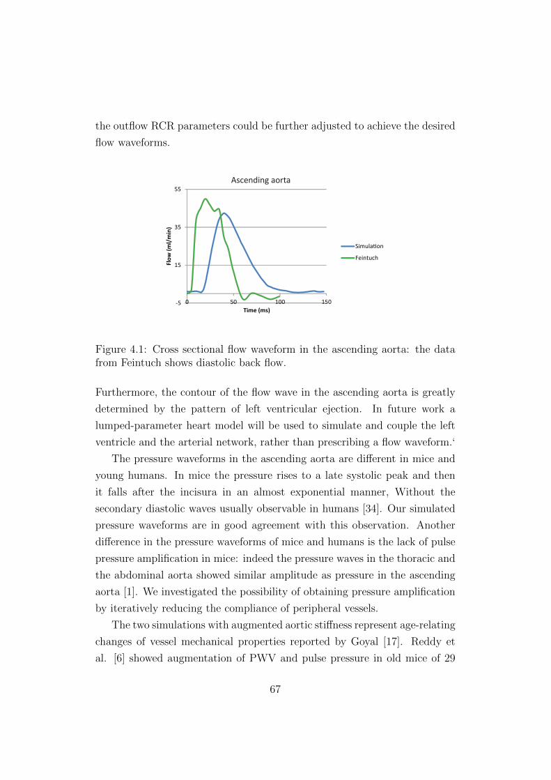
the outflow RCR parameters could be further adjusted to achieve the desired

flow waveforms.

-5

15

35

55

0 50 100 150

Flow

(ml/

min

)

Time (ms)

Simulation

Feintuch

Ascending aorta

Figure 4.1: Cross sectional flow waveform in the ascending aorta: the datafrom Feintuch shows diastolic back flow.

Furthermore, the contour of the flow wave in the ascending aorta is greatly

determined by the pattern of left ventricular ejection. In future work a

lumped-parameter heart model will be used to simulate and couple the left

ventricle and the arterial network, rather than prescribing a flow waveform.‘

The pressure waveforms in the ascending aorta are different in mice and

young humans. In mice the pressure rises to a late systolic peak and then

it falls after the incisura in an almost exponential manner, Without the

secondary diastolic waves usually observable in humans [34]. Our simulated

pressure waveforms are in good agreement with this observation. Another

difference in the pressure waveforms of mice and humans is the lack of pulse

pressure amplification in mice: indeed the pressure waves in the thoracic and

the abdominal aorta showed similar amplitude as pressure in the ascending

aorta [1]. We investigated the possibility of obtaining pressure amplification

by iteratively reducing the compliance of peripheral vessels.

The two simulations with augmented aortic stiffness represent age-relating

changes of vessel mechanical properties reported by Goyal [17]. Reddy et

al. [6] showed augmentation of PWV and pulse pressure in old mice of 29

67

months old compared to adult mice of 8 months old. The increase of PWV

with augmented stiffness is consistent with the Moens-Korteweg equation

which asserts that PWV is proportional to square root of young modulus E:

PWV =

√Eh

2rρ

Increasing vessel stiffness and decreasing compliance values of the Wind-

kessel model are two aspects of the same matter. Both contribute to decrease

the total compliance of the system and therefore to increase the pulse pres-

sure. However, this increase in pulse pressure is different in the two cases.

Indeed, decreasing the peripheral compliances results in pressure waveforms

exhibiting the same value in systole and lower diastolic values with increas-

ing distance from the ascending aorta. Therefore the augmentation of pulse

pressure is not spatially uniform. On the other hand, the case with increased

stiffness shows similar diastolic values and larger and larger systolic values.

An important limitation of this thesis is the uncertainty and the multiple

origins of the data utilized. A 3-D geometric model which does not exactly

correspond to the actual dimensions of a mice is a factor that could strongly

affect the results. The original 3-D geometry represented the qualitative

shape (branching patterns and vessel length) of the arterial tree but with in-

correct diameter dimensions; for this reason big part of the work consisted in

obtaining representative data in literature on vessel diameters. The scaling

of the original geometry was chosen to match the diameter average of each

vessel with the values reported in literature. The same uncertainty applies

to pressure. Pressure data in different locations were reported in different

papers; and even though mouse strain, age and weight could be comparable,

the experimental conditions are always different. This complicates the valida-

tion of pressure distributions in the simulations. Lastly, the tissue properties

were only known at four different locations, and had to be interpolated to

the entire model. Future work will involve considering the full biaxial data

rather than just the circumferential component.

The real innovations of this work are the reproduction of physiological

pressure waveforms and flow distribution in a realistic model of the mouse

68

vasculature.

69

Bibliography

[1] W. W. Nichols and M. F. ORourke, “Mcdonald’s blood flow in arteries.

theoretical, experimental and clinical principles,” Fourth edition, 1998.

[2] H. L. Lujan and S. E. Dicarlo, “Cardiac output, at rest and during exer-

cise, before and during myocardial ischemia, reperfusion, and infarction

in conscious mice.” American journal of physiology. Regulatory, inte-

grative and comparative physiology, vol. 304, no. 4, pp. R286–95, Feb.

2013.

[3] A. Feintuch, P. Ruengsakulrach, A. Lin, J. Zhang, Y.Q. Zhou, J. Bishop,

L. Davidson, D. Courtman, F. S. Foster, D. a. Steinman, R. M. Henkel-

man, and C. R. Ethier, “Hemodynamics in the mouse aortic arch as

assessed by MRI, ultrasound, and numerical modeling.” American jour-

nal of physiology. Heart and circulatory physiology, vol. 292, no. 2, pp.

H884–92, Feb. 2007.

[4] J. M. Greve, A. S. Les, B. T. Tang, M. T. Draney Blomme, N. M.

Wilson, R. L. Dalman, N. J. Pelc, and C. a. Taylor, “Allometric scal-

ing of wall shear stress from mice to humans: quantification using cine

phase-contrast MRI and computational fluid dynamics.” American jour-

nal of physiology. Heart and circulatory physiology, vol. 291, no. 4, pp.

H1700–8, Oct. 2006.

[5] A. K. Reddy, G. E. Taffet, J. F. Prchal, L. H. Michael, M. L. Ent-

man, and C. J. Hartley, “Effect of cellular elements on pressure-velocity

relationship in mice.” Annual International Conference of the IEEE En-

gineering in Medicine and Biology Society., vol. 5, pp. 3720–2, Jan. 2004.

70

[6] A. K. Reddy, Y.H. Li, T. T. Pham, L. N. Ochoa, M. T. Trevino, C. J.

Hartley, L. H. Michael, M. L. Entman, and G. E. Taffet, “Measurement

of aortic input impedance in mice: effects of age on aortic stiffness.”

American journal of physiology. Heart and circulatory physiology, vol.

285, no. 4, pp. H1464–70, Oct. 2003.

[7] B. N. Van Vliet, L. L. Chafe, and J.P. Montani, “Characteristics of 24

h telemetered blood pressure in eNOS-knockout and C57Bl/6J control

mice.” The Journal of physiology, vol. 549, pp. 313–25, May 2003.

[8] J. J. McGuire, B. N. Van Vliet, and S. J. Halfyard, “Blood pressures,

heart rate and locomotor activity during salt loading and angiotensin II

infusion in protease-activated receptor 2 (PAR2) knockout mice.” BMC

physiology, vol. 8, p. 20, Jan. 2008.

[9] B. Vandeghinste, B. Trachet, M. Renard, C. Casteleyn, S. Staelens,

B. Loeys, P. Segers, and S. Vandenberghe, “Replacing vascular corro-

sion casting by in vivo micro-CT imaging for building 3D cardiovascular

models in mice.” Molecular imaging and biology : MIB, vol. 13, no. 1,

pp. 78–86, Feb. 2011.

[10] C. Casteleyn, B. Trachet, D. Van Loo, D. G. H. Devos, W. Van den

Broeck, P. Simoens, and P. Cornillie, “Validation of the murine aortic

arch as a model to study human vascular diseases.” Journal of anatomy,

vol. 216, no. 5, pp. 563–71, May 2010.

[11] R. B. Hinton, C. M. Alfieri, S. A. Witt, B. J. Glascock, P. R. Khoury,

D. W. Benson, and K. E. Yutzey, “Mouse heart valve structure and

function: echocardiographic and morphometric analyses from the fetus

through the aged adult.” American journal of physiology. Heart and

circulatory physiology, vol. 294, no. 6, pp. H2480–8, Jun. 2008.

[12] W. Wan, H. Yanagisawa, and R. L. Gleason, “Biomechanical and mi-

crostructural properties of common carotid arteries from fibulin-5 null

mice.” Annals of biomedical engineering, vol. 38, no. 12, pp. 3605–17,

Dec. 2010.

71

[13] B. Trachet, M. Renard, G. De Santis, S. Staelens, J. De Backer,

L. Antiga, B. Loeys, and P. Segers, “An integrated framework to quan-

titatively link mouse-specific hemodynamics to aneurysm formation in

angiotensin II-infused ApoE -/- mice.” Annals of biomedical engineering,

vol. 39, no. 9, pp. 2430–44, Sep. 2011.

[14] X. Guo, Y. Kono, R. Mattrey, and G. S. Kassab, “Morphometry and

strain distribution of the C57BL/6 mouse aorta.” American journal of

physiology. Heart and circulatory physiology, vol. 283, no. 5, pp. H1829–

37, Nov. 2002.

[15] N. Xiao, J. Alastruey, and C. A. Figueroa, “A Systematic Comparison

between 1-D and 3-D Hemodynamics in Compliant Arterial Models,”

International Journal for Numerical Methods in Biomedical Enginering,

pp. 1–22, 2012.

[16] C. A. Figueroa, I. E. Vignon-Clementel, K. E. Jansen, T. J. Hughes, and

C. A. Taylor, “A coupled momentum method for modeling blood flow

in three-dimensional deformable arteries,” Computer Methods in Applied

Mechanics and Engineering, vol. 195, pp. 5685–5706, Aug. 2006.

[17] V. Goyal, “Change with age in the aorta of man and mouse,” Experi-

mental gerontology, vol. 17, pp. 127–132, 1982.

[18] British Heart foundation, University of Oxford, “European cardiouvas-

cular disease statistics,” 2012.

[19] V. M. Barodka, B. L. Joshi, D. E. Berkowitz, C. W. Hogue, and D. Ny-

han, “Implications of Vascular Aging,” vol. 112, no. 5, pp. 1048–1060,

2011.

[20] A. Redheuil, W.C. Yu, C. O. Wu, E. Mousseaux, A. D. Cesare,

N. Kachenoura, D. Bluemke, J. A. C. Lima, and R. Yan, “Reduced

Ascending Aortic Strain and Distensibility Earliest Manifestations of

Vascular Aging in Humans,” Hypertension, Journal of the American

heart association, pp. 319–326, 2010.

72

[21] J. S. Wilson, S. Baek, and J. D. Humphrey, “Importance of initial aortic

properties on the evolving regional anisotropy, stiffness and wall thick-

ness of human abdominal aortic aneurysms.” Journal of the Royal So-

ciety., vol. 9, no. 74, pp. 2047–58, Sep. 2012.

[22] E. G. Lakatta, M. Wang, and S. S. Najjar, “Arterial aging and subclin-

ical arterial disease are fundamentally intertwined at macroscopic and

molecular levels.” Med Clin North Am, vol. 93, no. 3, pp. 583–604, 2009.

[23] N. Xiao, J. D. Humphrey, and C. A. Figueroa, “Multi-scale computa-

tional model of three-dimensional hemodynamics within a deformable

full-body arterial network,” vol. 244, pp. 22–40, 2013.

[24] Y. Huo, X. Guo, and G. S. Kassab, “The flow field along the entire

length of mouse aorta and primary branches.” Annals of biomedical en-

gineering, vol. 36, no. 5, pp. 685–99, May 2008.

[25] I. E. Vignon and C. A. Taylor, “Outflow boundary conditions for one-

dimensional finite element modeling of blood flow and pressure waves in

arteries,” Wave Motion, vol. 39, no. 4, pp. 361–374, Apr. 2004.

[26] I. E. Vignon-Clementel, C. A. Figueroa, K. E. Jansen, and C. A. Taylor,

“Outflow boundary conditions for 3D simulations of non-periodic blood

flow and pressure fields in deformable arteries.” Computer methods in

biomechanics and biomedical engineering, vol. 13, no. 5, pp. 625–40, Oct.

2010.

[27] C. Tsukahara, F. Sugiyama, B. Paigen, S. Kunita, and K.-I. Yagami,

“Blood pressure in 15 inbred mouse strains and its lack of relation

with obesity and insulin resistance in the progeny of an NZO/HILtJ

x C3H/HeJ intercross.” Mammalian genome : official journal of the In-

ternational Mammalian Genome Society, vol. 15, no. 12, pp. 943–50,

Dec. 2004.

[28] J. N. Lorenz and E. G. Kranias, “Regulatory effects of phospholamban

on cardiac function in intact mice,” 2013.

73

[29] I. Giuvarasteanu, “Scanning electron microscopy of vascular corrosion

casts–standard method for studying microvessels.” Romanian journal of

morphology and embryology, vol. 48, no. 3, pp. 257–61, Jan. 2007.

[30] N. Wilson, K. Wang, R. W. Dutton, and C. Taylor, “A software frame-

work for creating patient specific geometric models from medical imag-

ing data for simulation based medical planning of vascular surgery,” in

MICCAI, 2001, pp. 449–456.

[31] I. E. Vignon-Clementel, C. A Figueroa, K. E. Jansen, and C. A. Tay-

lor, “Outflow boundary conditions for three-dimensional finite element

modeling of blood flow and pressure in arteries,” Computer Methods in

Applied Mechanics and Engineering, vol. 195, no. 29-32, pp. 3776–3796,

Jun. 2006.

[32] P. Moireau, N. Xiao, M. Astorino, C. A. Figueroa, D. Chapelle, C. A.

Taylor, and J.-F. Gerbeau, “External tissue support and fluid-structure

simulation in blood flows.” Biomechanics and modeling in mechanobiol-

ogy, vol. 11, no. 1-2, pp. 1–18, Jan. 2012.

[33] P. Reymond, F. Merenda, F. Perren, D. Rufenacht, and N. Stergiopulos,

“Validation of a one-dimensional model of the systemic arterial tree.”

American journal of physiology. Heart and circulatory physiology, vol.

297, no. 1, pp. H208–22, Jul. 2009.

[34] W. F. Hamilton and R. A. Woodbury, “Blood pressure studies in small

animals,” The American Journal of Physiology, vol. 119, 1937.

74