appendix - spatialtech.com.t9).pdf · 1/05 appendix • 9-1 9. appendix i. hypack® data types a....
TRANSCRIPT

1/05 Appendix •••• 9-1
9. Appendix
I. HYPACK® Data Types
A. HYPACK® Project File Types HYPACK® MAX has many types. Once you become experienced with the package, it will not be so overwhelming. The following gives a listing of file types and a brief description of each.
*.3DM 3D Terrain Viewer movie file. It contains information that, together with the corresponding XYZ data file, can replay a set of views recorded through the 3D Terrain Viewer program.
*.3DV 3D Terrain Viewer initialization file.
*.3OD 3D Object Design File created in the 3D SHAPE EDITOR, contains all of the information about all of the objects, their properties, etc. needed to create the *.VES file. To modify your *.VES file, you must re-open its *.30D file in the 3D SHAPE EDITOR, make your changes and export a new *.VES file.
*.BRD Border File: A border file is a listing of XY positions which can be used to clip data files in HYPACK® MAX and planned line files in the LINE EDITOR. It can be used to limit the area where MULTIBEAM MAX searches for data outside the search and filter criteria, and to limit the area where volumes are calculated in CROSS SECTIONS AND VOLUMES.
*.CHN Channel File: A channel design file contains a description of the geometry of an area. It is created in the ADVANCED CHANNEL DESIGN program and can be used in the TIN MODEL program to calculate the volume between a surveyed surface and the channel surface. A channel file can be displayed in MULTIBEAM MAX to guide the editing process.
*.COB Cross Section Object File contains the text, pipeline and polyline information for a cross section graph in CROSS SECTIONS AND VOLUMES and ADCP PROFILER.
*.CSS Cross Section Session File contains a list of files used in the CROSS SECTIONS AND VOLUMES program.
*.DCT Data Corrections Table information used in the Sounding Adjustment program to correct Sound Velocity Correction Values. The program adds the "fixed" corrections (not interpolated values) to the current sound velocity values in edited All format data.
*.DEP Digitized Depth File: A file of event marks versus depths. It is created in the ECHOGRAM digitizing program and can be used to merge depths with positions in the SINGLE BEAM EDITOR.
9-2 •••• Appendix 01/05
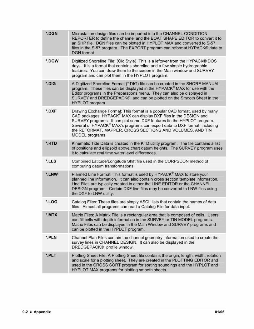
*.DGN Microstation design files can be imported into the CHANNEL CONDITION REPORTER to define the channel and the BOAT SHAPE EDITOR to convert it to an SHP file. DGN files can be plotted in HYPLOT MAX and converted to S-57 files in the S-57 program. The EXPORT program can reformat HYPACK® data to DGN format.
*.DGW Digitized Shoreline File: (Old Style) This is a leftover from the HYPACK® DOS days. It is a format that contains shoreline and a few simple hydrographic features. You can draw them to the screen in the Main window and SURVEY program and can plot them in the HYPLOT program.
*.DIG A Digitized Shoreline Format (*.DIG) file can be created in the SHORE MANUAL program. These files can be displayed in the HYPACK® MAX for use with the Editor programs in the Preparations menu. They can also be displayed in SURVEY and DREDGEPACK® and can be plotted on the Smooth Sheet in the HYPLOT program.
*.DXF Drawing Exchange Format: This format is a popular CAD format, used by many CAD packages. HYPACK® MAX can display DXF files in the DESIGN and SURVEY programs. It can plot some DXF features tin the HYPLOT program. Several of HYPACK® MAX's programs can export data to DXF format, including the REFORMAT, MAPPER, CROSS SECTIONS AND VOLUMES, AND TIN MODEL programs.
*.KTD Kinematic Tide Data is created in the KTD utility program. The file contains a list of positions and ellipsoid above chart datum heights. The SURVEY program uses it to calculate real time water level differences.
*.LLS Combined Latitude/Longitude Shift file used in the CORPSCON method of computing datum transformations.
*.LNW Planned Line Format: This format is used by HYPACK® MAX to store your planned line information. It can also contain cross section template information. Line Files are typically created in either the LINE EDITOR or the CHANNEL DESIGN program. Certain DXF line files may be converted to LNW files using the DXF to LNW utility.
*.LOG Catalog Files: These files are simply ASCII lists that contain the names of data files. Almost all programs can read a Catalog File for data input.
*.MTX Matrix Files: A Matrix File is a rectangular area that is composed of cells. Users can fill cells with depth information in the SURVEY or TIN MODEL programs. Matrix Files can be displayed in the Main Window and SURVEY programs and can be plotted in the HYPLOT program.
*.PLN Channel Plan Files contain the channel geometry information used to create the survey lines in CHANNEL DESIGN. It can also be displayed in the DREDGEPACK® profile window.
*.PLT Plotting Sheet File: A Plotting Sheet file contains the origin, length, width, rotation and scale for a plotting sheet. They are created in the PLOTTING EDITOR and used in the CROSS SORT program for sorting soundings and the HYPLOT and HYPLOT MAX programs for plotting smooth sheets.
1/05 Appendix •••• 9-3
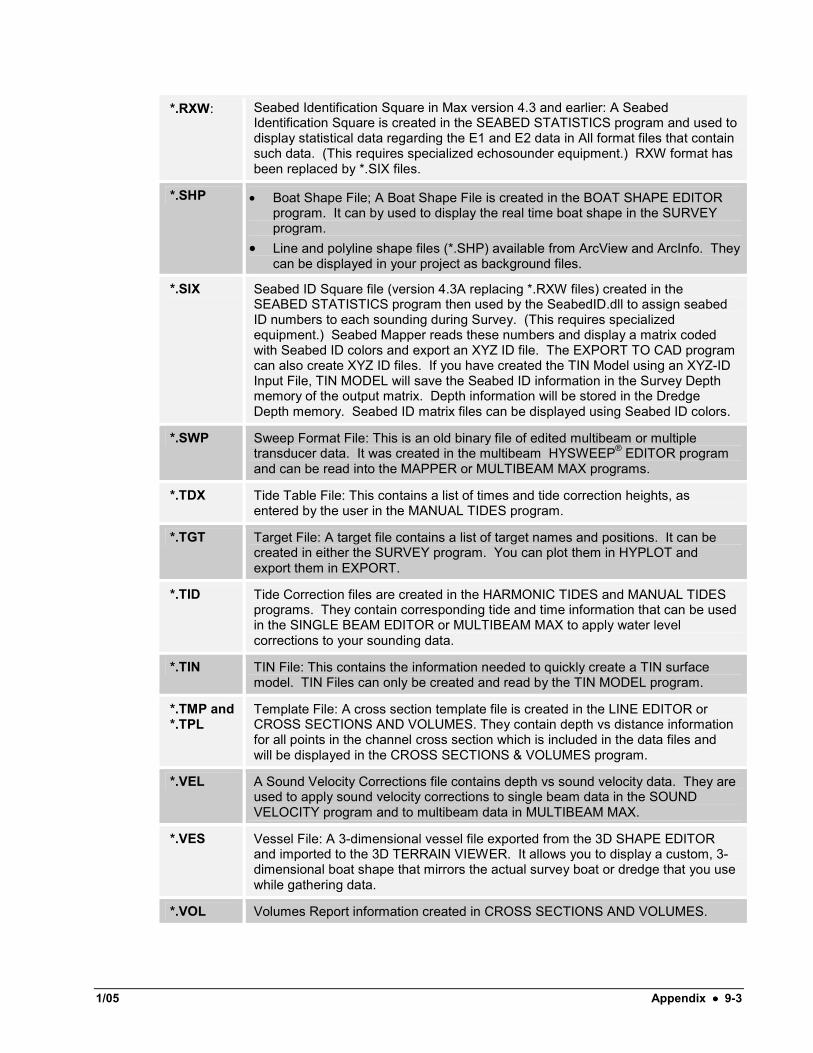
*.RXW: Seabed Identification Square in Max version 4.3 and earlier: A Seabed Identification Square is created in the SEABED STATISTICS program and used to display statistical data regarding the E1 and E2 data in All format files that contain such data. (This requires specialized echosounder equipment.) RXW format has been replaced by *.SIX files.
*.SHP • Boat Shape File; A Boat Shape File is created in the BOAT SHAPE EDITOR program. It can by used to display the real time boat shape in the SURVEY program.
• Line and polyline shape files (*.SHP) available from ArcView and ArcInfo. They can be displayed in your project as background files.
*.SIX Seabed ID Square file (version 4.3A replacing *.RXW files) created in the SEABED STATISTICS program then used by the SeabedID.dll to assign seabed ID numbers to each sounding during Survey. (This requires specialized equipment.) Seabed Mapper reads these numbers and display a matrix coded with Seabed ID colors and export an XYZ ID file. The EXPORT TO CAD program can also create XYZ ID files. If you have created the TIN Model using an XYZ-ID Input File, TIN MODEL will save the Seabed ID information in the Survey Depth memory of the output matrix. Depth information will be stored in the Dredge Depth memory. Seabed ID matrix files can be displayed using Seabed ID colors.
*.SWP Sweep Format File: This is an old binary file of edited multibeam or multiple transducer data. It was created in the multibeam HYSWEEP® EDITOR program and can be read into the MAPPER or MULTIBEAM MAX programs.
*.TDX Tide Table File: This contains a list of times and tide correction heights, as entered by the user in the MANUAL TIDES program.
*.TGT Target File: A target file contains a list of target names and positions. It can be created in either the SURVEY program. You can plot them in HYPLOT and export them in EXPORT.
*.TID Tide Correction files are created in the HARMONIC TIDES and MANUAL TIDES programs. They contain corresponding tide and time information that can be used in the SINGLE BEAM EDITOR or MULTIBEAM MAX to apply water level corrections to your sounding data.
*.TIN TIN File: This contains the information needed to quickly create a TIN surface model. TIN Files can only be created and read by the TIN MODEL program.
*.TMP and *.TPL
Template File: A cross section template file is created in the LINE EDITOR or CROSS SECTIONS AND VOLUMES. They contain depth vs distance information for all points in the channel cross section which is included in the data files and will be displayed in the CROSS SECTIONS & VOLUMES program.
*.VEL A Sound Velocity Corrections file contains depth vs sound velocity data. They are used to apply sound velocity corrections to single beam data in the SOUND VELOCITY program and to multibeam data in MULTIBEAM MAX.
*.VES Vessel File: A 3-dimensional vessel file exported from the 3D SHAPE EDITOR and imported to the 3D TERRAIN VIEWER. It allows you to display a custom, 3-dimensional boat shape that mirrors the actual survey boat or dredge that you use while gathering data.
*.VOL Volumes Report information created in CROSS SECTIONS AND VOLUMES.
9-4 •••• Appendix 01/05
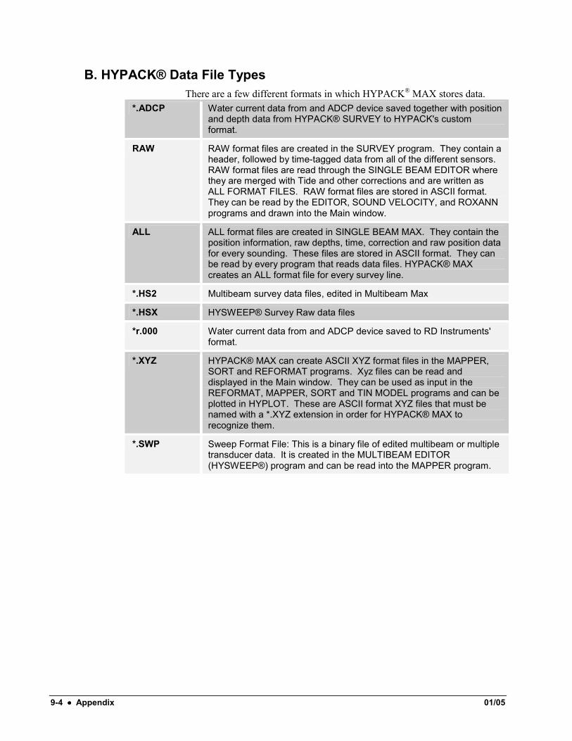
B. HYPACK® Data File Types There are a few different formats in which HYPACK® MAX stores data.
*.ADCP Water current data from and ADCP device saved together with position and depth data from HYPACK® SURVEY to HYPACK's custom format.
RAW RAW format files are created in the SURVEY program. They contain a header, followed by time-tagged data from all of the different sensors. RAW format files are read through the SINGLE BEAM EDITOR where they are merged with Tide and other corrections and are written as ALL FORMAT FILES. RAW format files are stored in ASCII format. They can be read by the EDITOR, SOUND VELOCITY, and ROXANN programs and drawn into the Main window.
ALL ALL format files are created in SINGLE BEAM MAX. They contain the position information, raw depths, time, correction and raw position data for every sounding. These files are stored in ASCII format. They can be read by every program that reads data files. HYPACK® MAX creates an ALL format file for every survey line.
*.HS2 Multibeam survey data files, edited in Multibeam Max
*.HSX HYSWEEP® Survey Raw data files
*r.000 Water current data from and ADCP device saved to RD Instruments' format.
*.XYZ HYPACK® MAX can create ASCII XYZ format files in the MAPPER, SORT and REFORMAT programs. Xyz files can be read and displayed in the Main window. They can be used as input in the REFORMAT, MAPPER, SORT and TIN MODEL programs and can be plotted in HYPLOT. These are ASCII format XYZ files that must be named with a *.XYZ extension in order for HYPACK® MAX to recognize them.
*.SWP Sweep Format File: This is a binary file of edited multibeam or multiple transducer data. It is created in the MULTIBEAM EDITOR (HYSWEEP®) program and can be read into the MAPPER program.
1/05 Appendix •••• 9-5
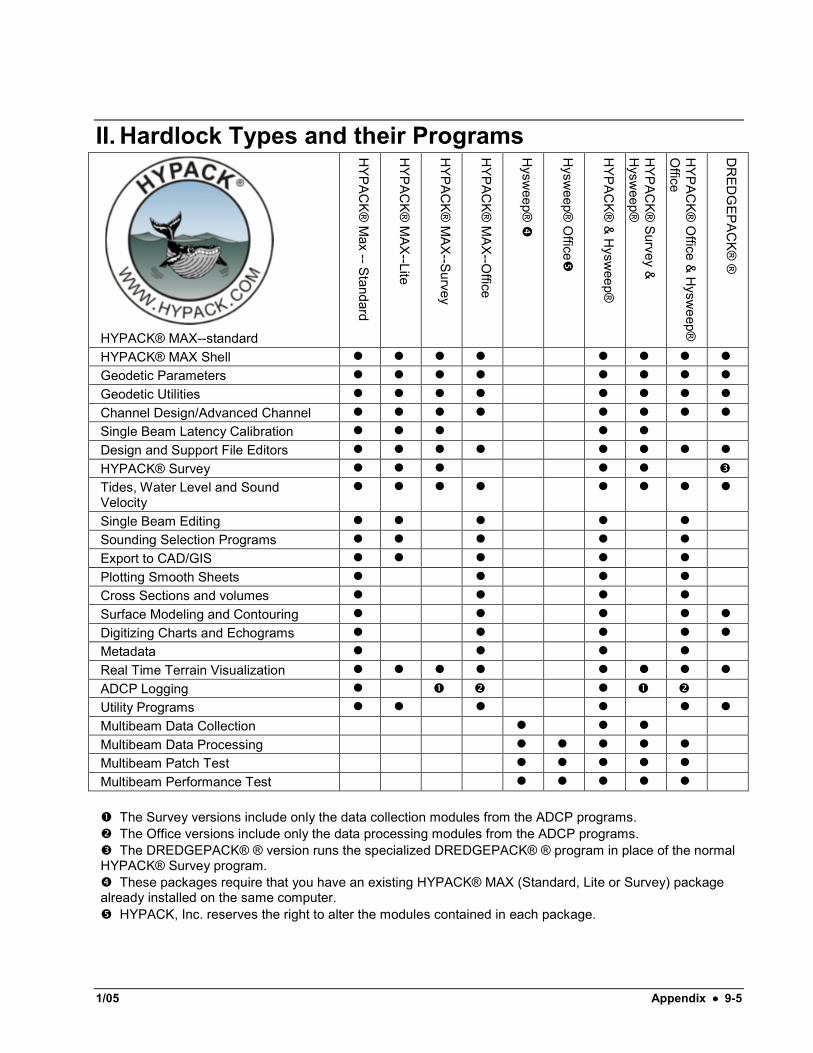
II. Hardlock Types and their Programs
HYPACK® MAX--standard
HYP
ACK®
Max -- Standard
HYP
ACK®
MA
X--Lite
HYP
ACK®
MA
X--Survey
HYP
ACK®
MA
X--Office
Hysw
eep®
Hysw
eep® O
ffice
HYP
ACK®
& Hysw
eep®
HYP
ACK®
Survey &
Hysw
eep®
HYP
ACK®
Office & H
ysweep®
O
ffice
DR
EDG
EPAC
K® ®
HYPACK® MAX Shell n n n n n n n n Geodetic Parameters n n n n n n n n Geodetic Utilities n n n n n n n n Channel Design/Advanced Channel n n n n n n n n Single Beam Latency Calibration n n n n n Design and Support File Editors n n n n n n n n HYPACK® Survey n n n n n Tides, Water Level and Sound Velocity
n n n n n n n n
Single Beam Editing n n n n n Sounding Selection Programs n n n n n Export to CAD/GIS n n n n n Plotting Smooth Sheets n n n n Cross Sections and volumes n n n n Surface Modeling and Contouring n n n n n Digitizing Charts and Echograms n n n n n Metadata n n n n Real Time Terrain Visualization n n n n n n n n ADCP Logging n n Utility Programs n n n n n n Multibeam Data Collection n n n Multibeam Data Processing n n n n n Multibeam Patch Test n n n n n Multibeam Performance Test n n n n n
The Survey versions include only the data collection modules from the ADCP programs. The Office versions include only the data processing modules from the ADCP programs. The DREDGEPACK® ® version runs the specialized DREDGEPACK® ® program in place of the normal
HYPACK® Survey program. These packages require that you have an existing HYPACK® MAX (Standard, Lite or Survey) package
already installed on the same computer. HYPACK, Inc. reserves the right to alter the modules contained in each package.
9-6 •••• Appendix 01/05
III. Keyboard Commands
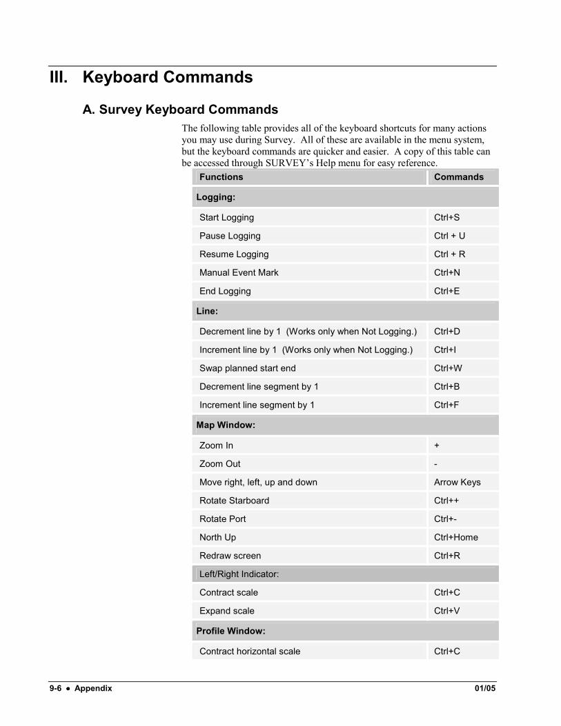
A. Survey Keyboard Commands The following table provides all of the keyboard shortcuts for many actions you may use during Survey. All of these are available in the menu system, but the keyboard commands are quicker and easier. A copy of this table can be accessed through SURVEY’s Help menu for easy reference.
Functions Commands
Logging:
Start Logging Ctrl+S
Pause Logging Ctrl + U
Resume Logging Ctrl + R
Manual Event Mark Ctrl+N
End Logging Ctrl+E
Line:
Decrement line by 1 (Works only when Not Logging.) Ctrl+D
Increment line by 1 (Works only when Not Logging.) Ctrl+I
Swap planned start end Ctrl+W
Decrement line segment by 1 Ctrl+B
Increment line segment by 1 Ctrl+F
Map Window:
Zoom In +
Zoom Out -
Move right, left, up and down Arrow Keys
Rotate Starboard Ctrl++
Rotate Port Ctrl+-
North Up Ctrl+Home
Redraw screen Ctrl+R
Left/Right Indicator:
Contract scale Ctrl+C
Expand scale Ctrl+V
Profile Window:
Contract horizontal scale Ctrl+C

1/05 Appendix •••• 9-7
Functions Commands
Expand horizontal scale Ctrl+V
Decrease Vertical scale Alt+C
Increase vertical scale Alt+V
Draft/Squat Correction:
Increment by current increment Alt+W
Decrement by current increment Alt+X
Tide Corrections:
Increment by current increment Alt+Y
Decrement by current increment Alt+Z
Anchors:
Drop Anchor Alt+Anchor#
Raise Anchor Alt+Anchor#
Targets:
Mark target at boat origin F5
Target Properties dialog F6
Marks a Waters Edge Target F7
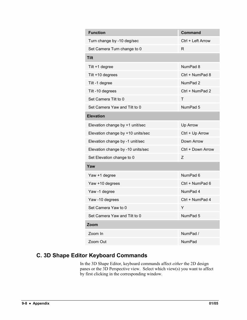
B. 3DTV Keyboard Commands Function Command
Pauses / Resumes camera motion Space bar
Stops all Camera motion NumPad 0
Speed
Increase Camera Speed by 1 unit/sec NumPad +
Decrease Camera Speed by 1 unit/sec NumPad -
Set Camera Speed to 0 S
Stop all camera motion NumPad 0
Turning
Turn change +1 deg/sec Right Arrow
Turn change by +10 deg/sec Ctrl + Right Arrow
Turn change -1 deg/sec Left Arrow
9-8 •••• Appendix 01/05
Function Command
Turn change by -10 deg/sec Ctrl + Left Arrow
Set Camera Turn change to 0 R
Tilt
Tilt +1 degree NumPad 8
Tilt +10 degrees Ctrl + NumPad 8
Tilt -1 degree NumPad 2
Tilt -10 degrees Ctrl + NumPad 2
Set Camera Tilt to 0 T
Set Camera Yaw and Tilt to 0 NumPad 5
Elevation
Elevation change by +1 unit/sec Up Arrow
Elevation change by +10 units/sec Ctrl + Up Arrow
Elevation change by -1 unit/sec Down Arrow
Elevation change by -10 units/sec Ctrl + Down Arrow
Set Elevation change to 0 Z
Yaw
Yaw +1 degree NumPad 6
Yaw +10 degrees Ctrl + NumPad 6
Yaw -1 degree NumPad 4
Yaw -10 degrees Ctrl + NumPad 4
Set Camera Yaw to 0 Y
Set Camera Yaw and Tilt to 0 NumPad 5
Zoom
Zoom In NumPad /
Zoom Out NumPad
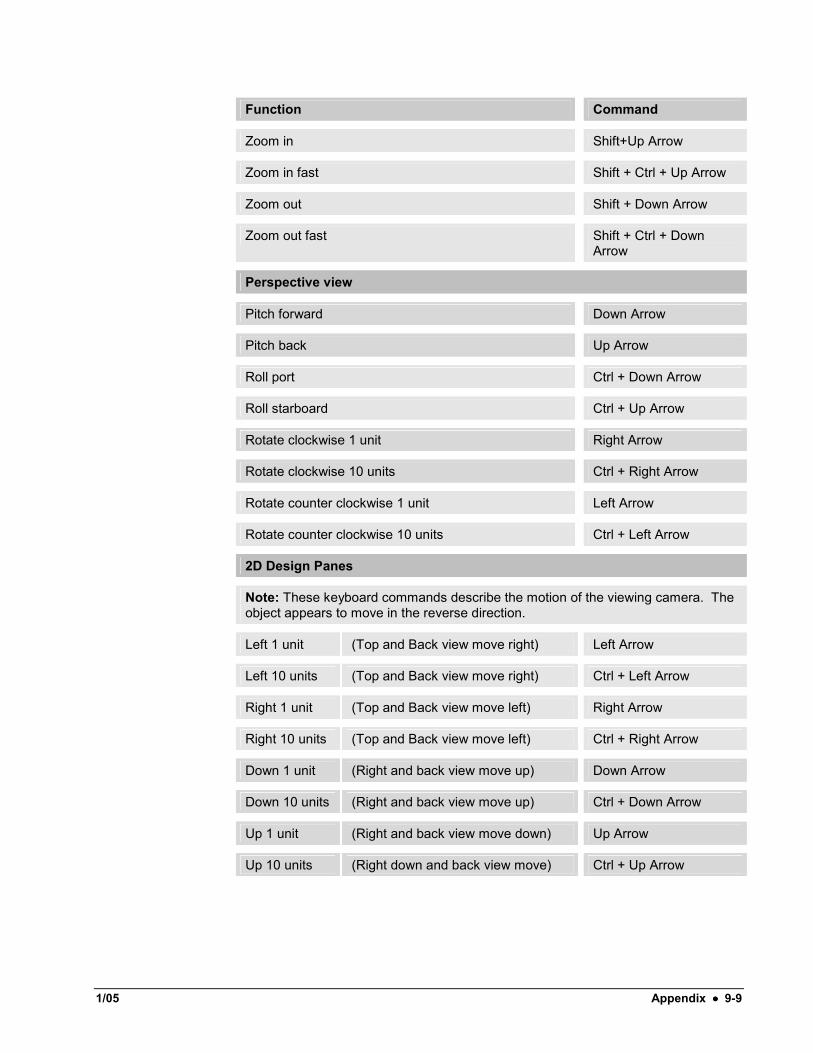
C. 3D Shape Editor Keyboard Commands In the 3D Shape Editor, keyboard commands affect either the 2D design panes or the 3D Perspective view. Select which view(s) you want to affect by first clicking in the corresponding window.
1/05 Appendix •••• 9-9
Function Command
Zoom in Shift+Up Arrow
Zoom in fast Shift + Ctrl + Up Arrow
Zoom out Shift + Down Arrow
Zoom out fast Shift + Ctrl + Down Arrow
Perspective view
Pitch forward Down Arrow
Pitch back Up Arrow
Roll port Ctrl + Down Arrow
Roll starboard Ctrl + Up Arrow
Rotate clockwise 1 unit Right Arrow
Rotate clockwise 10 units Ctrl + Right Arrow
Rotate counter clockwise 1 unit Left Arrow
Rotate counter clockwise 10 units Ctrl + Left Arrow
2D Design Panes
Note: These keyboard commands describe the motion of the viewing camera. The object appears to move in the reverse direction.
Left 1 unit (Top and Back view move right) Left Arrow
Left 10 units (Top and Back view move right) Ctrl + Left Arrow
Right 1 unit (Top and Back view move left) Right Arrow
Right 10 units (Top and Back view move left) Ctrl + Right Arrow
Down 1 unit (Right and back view move up) Down Arrow
Down 10 units (Right and back view move up) Ctrl + Down Arrow
Up 1 unit (Right and back view move down) Up Arrow
Up 10 units (Right down and back view move) Ctrl + Up Arrow
9-10 •••• Appendix 01/05
IV. Hardware Interfacing The key to successful operation of the SURVEY program is proper equipment interface with the survey computer. This means: • Having the correct hardware in your computer. • Making sure that hardware is properly configured. • Making sure your cable is correct • Correctly specifying the communication parameters for each piece of
survey equipment. • Survey equipment normally communicates over one of the following
communication protocols: ▪ Serial (RS-232, RS-422 and RS-485) ▪ Parallel (Centronics) ▪ Binary Coded Decimal (BCD) ▪ GPIB (IEEE-488) ▪ Analog ▪ Network (TCP\IP and UDP)
• Details of working with the different types of devices are provided in the following sub-sections.
A. Serial Interfacing For serial communication to succeed, the communication parameters must be configured in HARDWARE for each device. They must be set to match your equipment or you don’t have any chance to read the device in the SURVEY program.
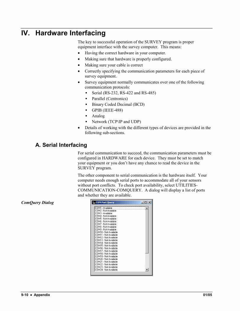
The other component to serial communication is the hardware itself. Your computer needs enough serial ports to accommodate all of your sensors without port conflicts. To check port availability, select UTILITIES-COMMUNICATION-COMQUERY. A dialog will display a list of ports and whether they are available.
ComQuery Dialog
1/05 Appendix •••• 9-11
Some devices are made so you can feed the data from one, through the other to the computer on one serial port. For example, GPS units commonly send their data through echosounders and gyros. This is called multiplexing. In this case, each of the device drivers would be set to the same COM port.
1) Communication Parameters Serial interfacing can be compared to running a single pipeline. Survey information is broken into individual characters, which are then broken down into a series of ones and zeroes. These ones and zeroes are known as bits. Each one or zero is transmitted by changing the voltage on a transmit wire. Your survey equipment may change the voltage to 5V to designate a zero, and then drop the voltage to 0V to designate a one.
Data bits and Stop bits This series of bits is normally transmitted in series of seven or eight data bits. Each hardware device will have a setting called data bits, which defines the number of bits in each group. At the end of each group, the device inserts one or more Stop bits. This provides the equipment with a little time to process each message and prepare for the next message.
Parity When serial transmission was first implemented, it was not as perfected as it is today. In order to check whether or not a message was correctly received, transmitting equipment would add a Parity bit. This was a single bit which would be either a zero or a one, depending on the sum of the data bits in the message group. • If you selected Even Parity, the parity bit would be set so the sum of all
of the data bits and parity bit would be an even number. • If you selected Odd Parity, the parity bit would be set so the sum of all
of the data bits and parity bit would be an odd number. This gave the receiving equipment a 50/50 chance of detecting a bad data group.
As serial equipment became more reliable, manufacturers began to eliminate the parity bit. In this case, a setting of None or No Parity would tell the devices not to worry about a parity bit.
Baud Rate The final essential piece of information needed to establish communication between two devices is the Baud Rate. This is the speed, expressed in bits per second, with which the two devices send characters to each other. In order to successfully communicate, both devices need to agree as to the Baud Rate, the Data bits, Stop bits and Parity. If any of these values are not specified correctly, the results may vary. For example, if you incorrectly specify the baud rate, your computer will receive what it thinks is gibberish. If you incorrectly specify the number of Stop bits, it may be able to successfully decipher 80% of the received messages.
Handshaking The other key, essential in serial communications is called Handshaking. This is how one device tells another device that it is either ready or not ready to receive additional information. For example, most computers can send information to a plotter faster than the plotter is capable of processing it. The plotter, first, stores information in a temporary buffer until it can process it. Once the buffer becomes full, it needs some way of telling the computer to stop sending the information. This is done via Handshaking. Handshaking is normally accomplished by one of the following methods:
9-12 •••• Appendix 01/05
Xon/Xoff is preferred by some devices because it requires no additional wires, other than a transmit, receive and signal ground wires. When a device is becoming full, it sends an Xoff character (CHR$17). Upon receipt, the transmitting device stops sending information. Once the receiving device has processed enough information and can receive more information, it sends an Xon character (CHR$19). This allows the transmitting device to resume its transmission. For equipment requiring this type of handshaking, set the Flow Control to software in the COM properties dialog.
CTS/RTS (Clear to Send/Ready to Send) and DST/DTR (Data Set Ready/Data Terminal Ready) are similar methods. They each require up to two additional wires in the serial cable. The transmitting device uses one wire to tell the receiving device it is ready to send data. The receiving device uses the other wire to tell the transmitting device it is ready to receive data. If one, or both, of the conditions are not met, the device does not transmit. HYPACK® MAX supports CTS/RTS handshaking when the Flow Control in the COM properties dialog is set to "hardware". Devices that require DST/DTR handshaking are a little different. The Flow Control is still set to "hardware", but you will also need a custom cable. The cable must connect the HYPACK® MAX RTS pin to the device DSR pin, and the HYPACK® MAX CTS pin to the device DTR pin for the devices to communicate.
In HYPACK® MAX, we prefer that all handshaking be set to None. This means that as soon as a measurement is made, it is transmitted to the computer without any additional delay. Unless there are overriding reasons, all equipment, with the exception of plotters, should be set with no handshaking.
2) Serial Hardware Now that your communication parameters are set correctly, let’s look at serial hardware.
All serial ports in your computer are referenced by a location (I/O Address) and how they tell the processor they need attention (Interrupt Request or IRQ). Serial ports are referred to as COM ports. The first on will be called COM1:, the second one COM2:, etc. Back in the 1980’s, there wasn’t a lot of thought about running multiple serial devices. It was expected that the maximum number of serial device that you might ever work with was four. It was defined that the following settings would apply for these four ports:
Name I/O Address IRQ
COM1: 3f8H 4
COM2: 2F8H 3
COM3: 3f8H 4
COM4: 2F8H 3
COM1: and COM3: shared the same IRQ, as did COM2: and COM4:. It was expected that you would not use the serial ports with the same interrupt at the same time. Problems arise when the CPU has more than one device on the same interrupt. It cannot figure out which one it needs to service and

1/05 Appendix •••• 9-13
“freezes”. If you experience frequent “freezing” of the SURVEY program, it is normally caused by serial port IRQ conflicts. Purchasing special serial ports that can be configured to different interrupts or are designed to share interrupts can eliminate this. Contact HYPACK, Inc. for details about serial cards that have this capability.
Many of you prefer to use notebook computers in field operations. Since most notebooks now come with only one serial port, additional serial ports can be added by using special PCMCIA serial cards. These cards, available from Quatech and other companies, come with one, two or four serial ports on a single card. Installing these cards in Windows® ’95 systems or newer notebooks is quite simple.
B. Binary Coded Decimal (BCD) Devices Where serial communications sends a series of ones and zeroes over a single wire, a BCD device sends groups of data over several wires. Each digit in a measurement is broken into a combination of 1-2-4-8 wires to signify different values. The benefit of BCD equipment is it can send entire depths or values at a single instance, where serial data requires a stream of ones and zeroes. The drawback is that BCD equipment requires data cables with many wires, it requires a special interface card, and normally cannot be used to annotate echosounders with text information.
Most BCD devices used in HYPACK® MAX are either older echosounders or magnetometers. In desktop systems, they are interfaced with a PIO-12 or PIO-24 interface card from Keithley-Metrabyte. In notebook systems, they are interfaced with an IOP-241 PCMCIA card from Quatech. These cards can be ordered from these companies or from HYPACK, Inc.. Contact the Sales Department for information on these cards.
Both of these cards will require that you fabricate a cable as per our instructions. Just because your BCD Atlas Deso 20 talked over a cable to your old HP system does not mean it will talk to a PC system using the same cable. Contact Tech Support to obtain cable specifications for the different BCD equipment.
Most BCD equipment uses a Strobe signal to notify the computer that a new measurement is available. Unless a Data Hold line is in use, the equipment then sends the information out the 1-2-4-8 data lines. Some equipment has a Bad Data line that is used to notify the computer that something is amiss with the value. Some equipment also has an Event Mark line. The computer uses this to trigger an event mark on the equipment. There is no provision in HYPACK® MAX to annotate BCD equipment.
C. GPIB Interfaces GPIB, also known as IEEE-448, was a popular interface when HP computers ruled the data collection world. It was a powerful interface, which allowed several devices to be “daisy chained” or connected back-to-back to a single GPIB port on your computer.
9-14 •••• Appendix 01/05
GPIB did not transfer gracefully to the PC computer world. For many years, it was necessary to purchase a “high end” interface card (translation: Expensive) and have a custom interface written for any GPIB device.
It is much easier today. Many companies offer GPIB interface cards that can be configured to appear as a serial port in Windows® ’95 and ’98. You can then integrate to these cards and configure them in HYPACK® MAX by selecting the name of the serial port (e.g. COM2:) which has been assigned to the GPIB card. The interface driver delivered with the card then takes over the task of interfacing the GPIB card to the operating system.
V. Drivers and their Devices
A. Device Drivers HYPACK® MAX can communicate with about 180 different types of survey equipment. This includes positioning systems, echosounders, motion sensors, gyros, tide gauges, magnetometers, and other pieces of survey equipment. If all of this code were built into the SURVEY program, it would be huge, requiring faster, more powerful computers to operate it.
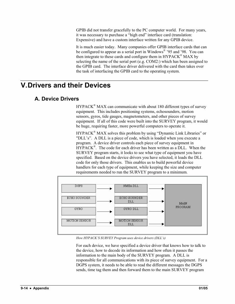
HYPACK® MAX solves this problem by using “Dynamic Link Libraries” or "DLL’s”. A DLL is a piece of code, which is loaded when you execute a program. A device driver controls each piece of survey equipment in HYPACK®. The code for each driver has been written as a DLL. When the SURVEY program starts, it looks to see what type of equipment you have specified. Based on the device drivers you have selected, it loads the DLL code for only those drivers. This enables us to build powerful device handlers for each type of equipment, while keeping the size and computer requirements needed to run the SURVEY program to a minimum.
How HYPACK’S SURVEY Program uses device drivers (DLL’s)
For each device, we have specified a device driver that knows how to talk to the device, how to decode its information and how often it passes the information to the main body of the SURVEY program. A DLL is responsible for all communications with its piece of survey equipment. For a DGPS system, it needs to be able to read the different messages the DGPS sends, time tag them and then forward them to the main SURVEY program
1/05 Appendix •••• 9-15
when requested. The DLL also sends messages from the Main program back to the survey device. An example of this would be the passing of annotation information to an echosounder.
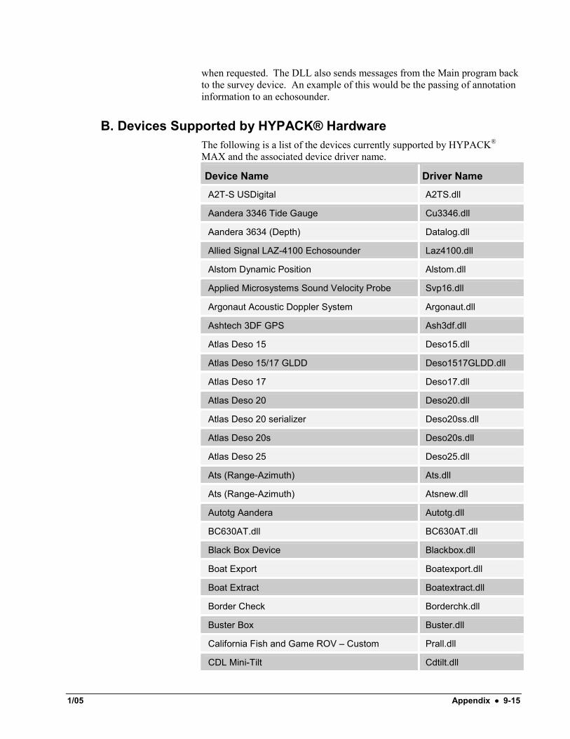
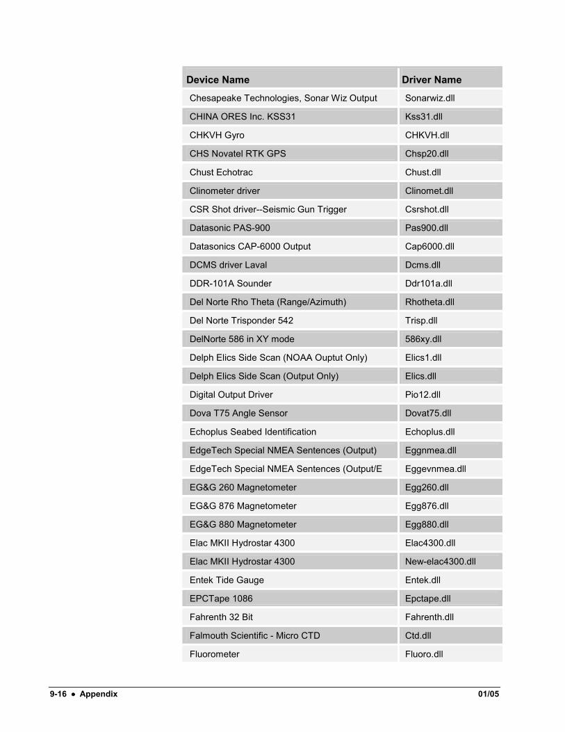
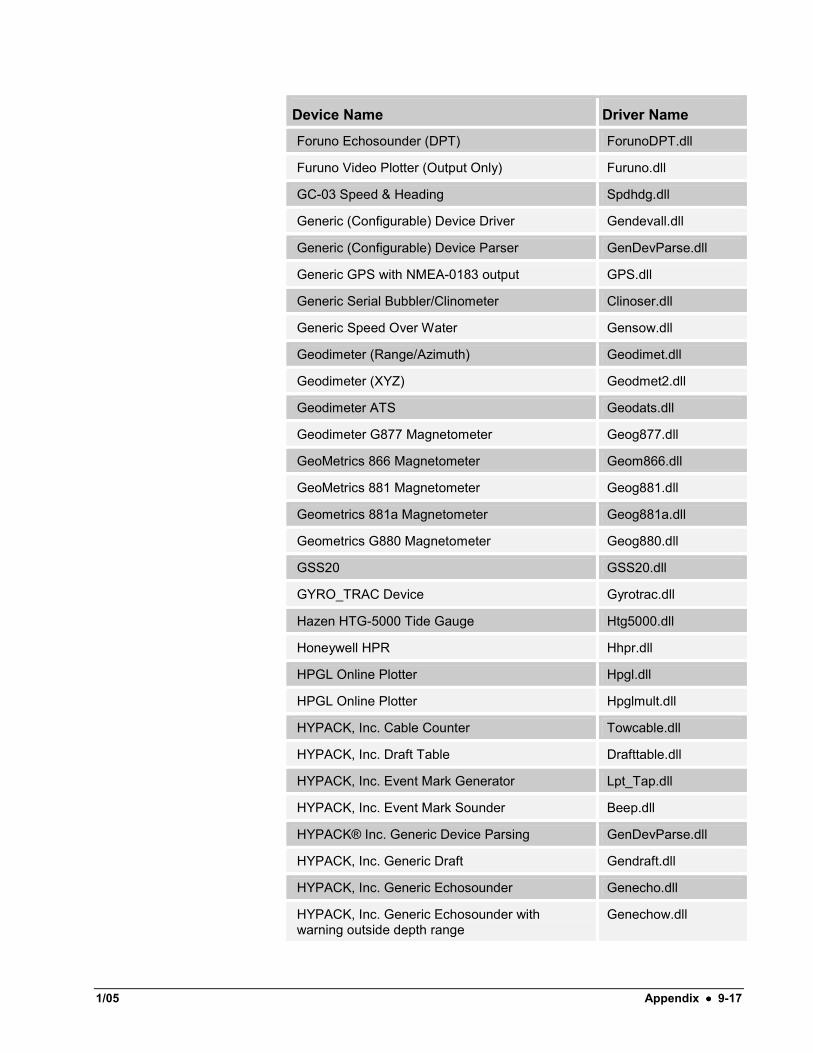
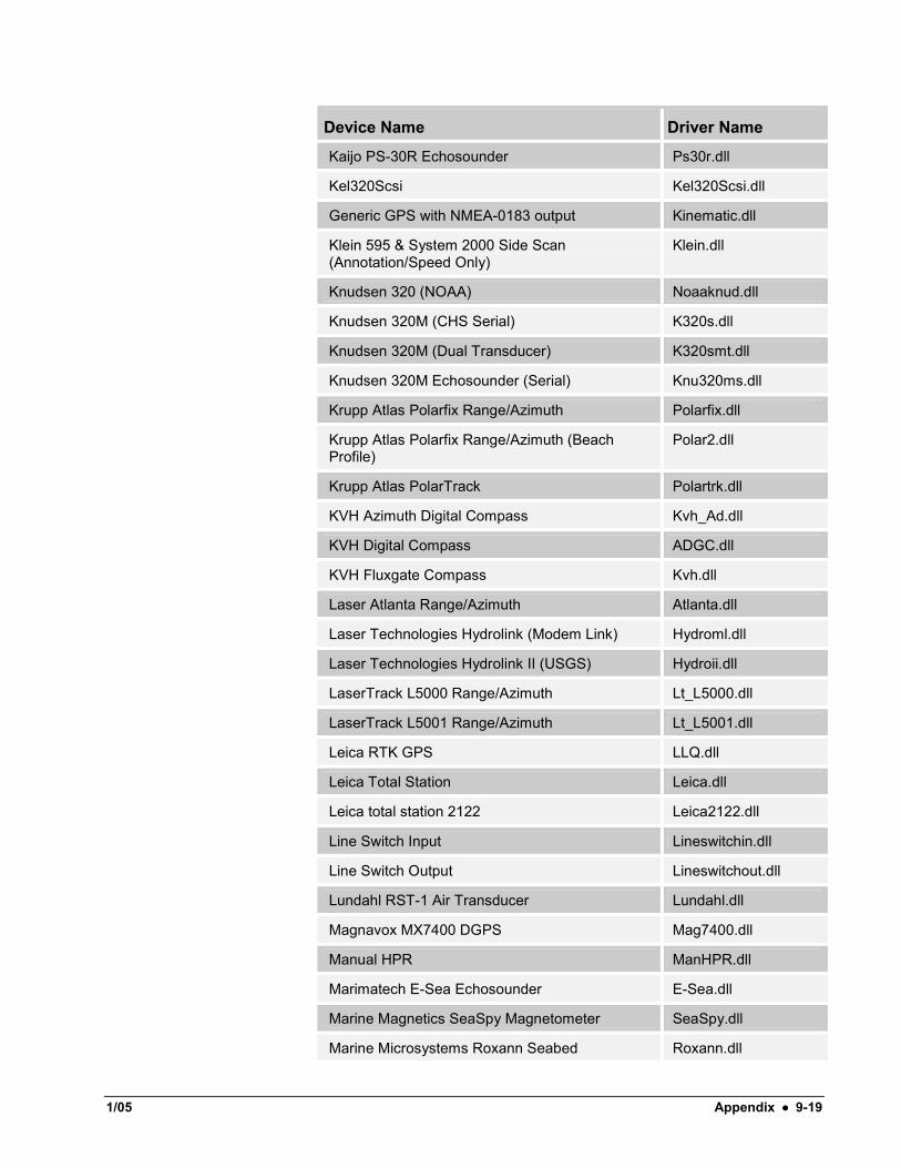
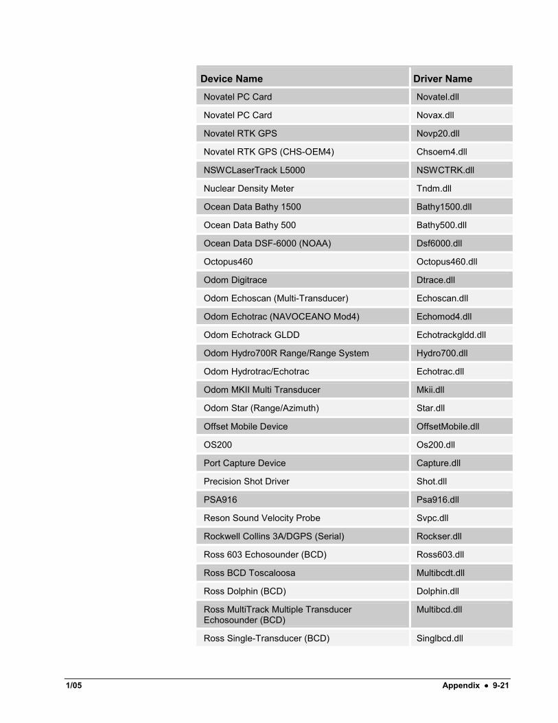
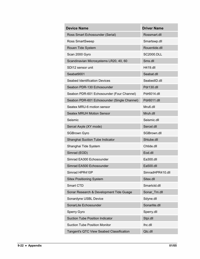
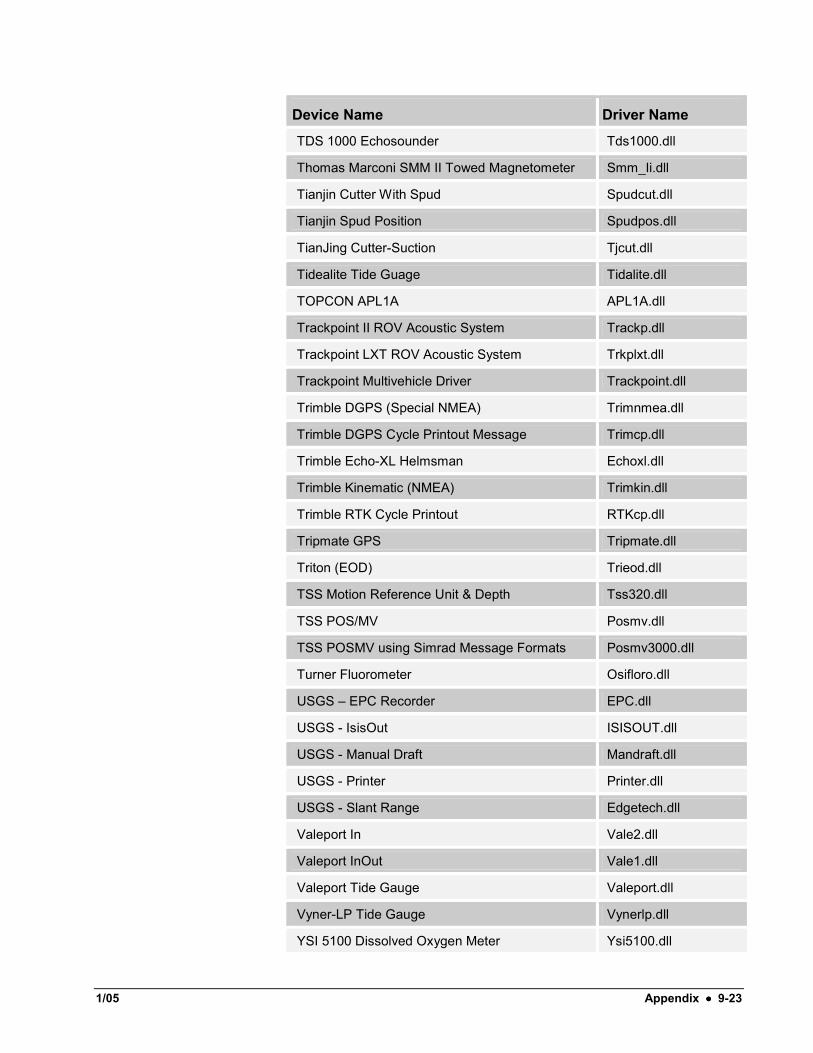
B. Devices Supported by HYPACK® Hardware The following is a list of the devices currently supported by HYPACK® MAX and the associated device driver name.
Device Name Driver Name
A2T-S USDigital A2TS.dll
Aandera 3346 Tide Gauge Cu3346.dll
Aandera 3634 (Depth) Datalog.dll
Allied Signal LAZ-4100 Echosounder Laz4100.dll
Alstom Dynamic Position Alstom.dll
Applied Microsystems Sound Velocity Probe Svp16.dll
Argonaut Acoustic Doppler System Argonaut.dll
Ashtech 3DF GPS Ash3df.dll
Atlas Deso 15 Deso15.dll
Atlas Deso 15/17 GLDD Deso1517GLDD.dll
Atlas Deso 17 Deso17.dll
Atlas Deso 20 Deso20.dll
Atlas Deso 20 serializer Deso20ss.dll
Atlas Deso 20s Deso20s.dll
Atlas Deso 25 Deso25.dll
Ats (Range-Azimuth) Ats.dll
Ats (Range-Azimuth) Atsnew.dll
Autotg Aandera Autotg.dll
BC630AT.dll BC630AT.dll
Black Box Device Blackbox.dll
Boat Export Boatexport.dll
Boat Extract Boatextract.dll
Border Check Borderchk.dll
Buster Box Buster.dll
California Fish and Game ROV – Custom Prall.dll
CDL Mini-Tilt Cdtilt.dll
9-16 •••• Appendix 01/05
Device Name Driver Name
Chesapeake Technologies, Sonar Wiz Output Sonarwiz.dll
CHINA ORES Inc. KSS31 Kss31.dll
CHKVH Gyro CHKVH.dll
CHS Novatel RTK GPS Chsp20.dll
Chust Echotrac Chust.dll
Clinometer driver Clinomet.dll
CSR Shot driver--Seismic Gun Trigger Csrshot.dll
Datasonic PAS-900 Pas900.dll
Datasonics CAP-6000 Output Cap6000.dll
DCMS driver Laval Dcms.dll
DDR-101A Sounder Ddr101a.dll
Del Norte Rho Theta (Range/Azimuth) Rhotheta.dll
Del Norte Trisponder 542 Trisp.dll
DelNorte 586 in XY mode 586xy.dll
Delph Elics Side Scan (NOAA Ouptut Only) Elics1.dll
Delph Elics Side Scan (Output Only) Elics.dll
Digital Output Driver Pio12.dll
Dova T75 Angle Sensor Dovat75.dll
Echoplus Seabed Identification Echoplus.dll
EdgeTech Special NMEA Sentences (Output) Eggnmea.dll
EdgeTech Special NMEA Sentences (Output/E Eggevnmea.dll
EG&G 260 Magnetometer Egg260.dll
EG&G 876 Magnetometer Egg876.dll
EG&G 880 Magnetometer Egg880.dll
Elac MKII Hydrostar 4300 Elac4300.dll
Elac MKII Hydrostar 4300 New-elac4300.dll
Entek Tide Gauge Entek.dll
EPCTape 1086 Epctape.dll
Fahrenth 32 Bit Fahrenth.dll
Falmouth Scientific - Micro CTD Ctd.dll
Fluorometer Fluoro.dll
1/05 Appendix •••• 9-17
Device Name Driver Name
Foruno Echosounder (DPT) ForunoDPT.dll
Furuno Video Plotter (Output Only) Furuno.dll
GC-03 Speed & Heading Spdhdg.dll
Generic (Configurable) Device Driver Gendevall.dll
Generic (Configurable) Device Parser GenDevParse.dll
Generic GPS with NMEA-0183 output GPS.dll
Generic Serial Bubbler/Clinometer Clinoser.dll
Generic Speed Over Water Gensow.dll
Geodimeter (Range/Azimuth) Geodimet.dll
Geodimeter (XYZ) Geodmet2.dll
Geodimeter ATS Geodats.dll
Geodimeter G877 Magnetometer Geog877.dll
GeoMetrics 866 Magnetometer Geom866.dll
GeoMetrics 881 Magnetometer Geog881.dll
Geometrics 881a Magnetometer Geog881a.dll
Geometrics G880 Magnetometer Geog880.dll
GSS20 GSS20.dll
GYRO_TRAC Device Gyrotrac.dll
Hazen HTG-5000 Tide Gauge Htg5000.dll
Honeywell HPR Hhpr.dll
HPGL Online Plotter Hpgl.dll
HPGL Online Plotter Hpglmult.dll
HYPACK, Inc. Cable Counter Towcable.dll
HYPACK, Inc. Draft Table Drafttable.dll
HYPACK, Inc. Event Mark Generator Lpt_Tap.dll
HYPACK, Inc. Event Mark Sounder Beep.dll
HYPACK® Inc. Generic Device Parsing GenDevParse.dll
HYPACK, Inc. Generic Draft Gendraft.dll
HYPACK, Inc. Generic Echosounder Genecho.dll
HYPACK, Inc. Generic Echosounder with warning outside depth range
Genechow.dll

9-18 •••• Appendix 01/05
Device Name Driver Name
HYPACK, Inc. Generic Gyro Gengyro.dll
HYPACK, Inc. Generic Offsets Genoffset.dll
HYPACK, Inc. Generic Simulator Sim32.dll
HYPACK, Inc. Generic Tide Gauge Gentide.dll
HYPACK, Inc. Generic XY Generxy.dll
HYPACK, Inc. Generic XYZ XYZ.dll
HYPACK, Inc. GPS Compare GpsComp.dll
HYPACK, Inc. HYSWEEP® Interface Hysweep.dll
HYPACK, Inc. LCD3 Helmsman Lcd3.dll
HYPACK, Inc. LCD4 Helmsman Lcd4.dll
HYPACK, Inc. Manual Entry Manual.dll
HYPACK, Inc. OTF-Gyro/Comparison OTFGyro.dll
HYPACK, Inc.' OutInfo OutInfo.dll
HYPACK, Inc. Playback driver Playback.dll
HYPACK, Inc. Simulation (Range-Azimuth/Sounder)
Testdev.dll
HYPACK, Inc. Tides (From File) Tidefile.dll
Innerspace 455 Inn455b.dll
Innerspace 455 (and 456) Inn455.dll
Innerspace 440 Echosounder (Serial) Inn440s.dll
Innerspace 448 Echosounder (Serial) Inn448.dll
Innerspace 449 Echosounder (Serial) Inn449.dll
Innerspace 449 rev. 2 Inn449R2.dll
Innerspace 449 Rev. 2 (Serial) Inn449rev2.dll
Innerspace 449Rc Inn449DFZ.dll
Innerspace 455 Inn455.dll
Innerspace LCD Helmsman InnLCD.dll
Isis (Triton) Custom EOD Isiseod.dll
Isis (Triton) Dynamic Data Exchange Interface Hdde.dll
IT2000 Series Intelligent Pressure Transducer IT2000.dll
Kaijo PS-20R Echosounder Ps20r.dll
1/05 Appendix •••• 9-19
Device Name Driver Name
Kaijo PS-30R Echosounder Ps30r.dll
Kel320Scsi Kel320Scsi.dll
Generic GPS with NMEA-0183 output Kinematic.dll
Klein 595 & System 2000 Side Scan (Annotation/Speed Only)
Klein.dll
Knudsen 320 (NOAA) Noaaknud.dll
Knudsen 320M (CHS Serial) K320s.dll
Knudsen 320M (Dual Transducer) K320smt.dll
Knudsen 320M Echosounder (Serial) Knu320ms.dll
Krupp Atlas Polarfix Range/Azimuth Polarfix.dll
Krupp Atlas Polarfix Range/Azimuth (Beach Profile)
Polar2.dll
Krupp Atlas PolarTrack Polartrk.dll
KVH Azimuth Digital Compass Kvh_Ad.dll
KVH Digital Compass ADGC.dll
KVH Fluxgate Compass Kvh.dll
Laser Atlanta Range/Azimuth Atlanta.dll
Laser Technologies Hydrolink (Modem Link) Hydroml.dll
Laser Technologies Hydrolink II (USGS) Hydroii.dll
LaserTrack L5000 Range/Azimuth Lt_L5000.dll
LaserTrack L5001 Range/Azimuth Lt_L5001.dll
Leica RTK GPS LLQ.dll
Leica Total Station Leica.dll
Leica total station 2122 Leica2122.dll
Line Switch Input Lineswitchin.dll
Line Switch Output Lineswitchout.dll
Lundahl RST-1 Air Transducer Lundahl.dll
Magnavox MX7400 DGPS Mag7400.dll
Manual HPR ManHPR.dll
Marimatech E-Sea Echosounder E-Sea.dll
Marine Magnetics SeaSpy Magnetometer SeaSpy.dll
Marine Microsystems Roxann Seabed Roxann.dll

9-20 •••• Appendix 01/05
Device Name Driver Name Identification
MD TOTCO Series 2000 Mdtotco.dll
MD4S Depth Device MD4S.dll
Measurement Technology NW LCI-90 Lci90.dll
Meconaut Bubbler System Meconaut.dll
Minesens Minesens.dll
Motorola Falcon Falcon.dll
Motorola Falcon IV Range/Range Falcon4.dll
Motorola Miniranger III (NM788 Serial Interface) Nm788.dll
Motorola Sixgun DGPS Sixgun.dll
Navisound 200/400 Series Navisound.dll
Navisound 210 Navsound210.dll
Navitron Sound50 Echosounder Sound50.dll
Navitronic Sounding 30 Echosounder Sdig30.dll
Navitronics Dpp1b Serial Echosounder Dpp1b.dll
Navitronics DPP2B Dpp2b.dll
Navitronics MCS2000 MCS2000.dll
Navitronics MCS2000-PWGSC Moncton Dpp2000.dll
Navitronics PGU-1000 Pgu1000.dll
NMEA Auto Pilot Autop.dll
NMEA In Klein Out Nmeakl.dll
NMEA Kinematic DGPS (Real Time Tides) Kin.dll
NMEA Server Client Nmeasc.dll
NMEA SSB Position Device SSB.dll
NMEA TKV Message (Speed/Temp) Nmeatkv.dll
NMEA-0183 Standard GPS Nmea.dll
Nmea-UDP Netnmea.dll
NOAA Cable Counter Cablecnt.dll
NOAA Delph Output Delph.dll
NOAA Isis Isis.dll
Novatel DGPS - OEM Card Novoem.dll
1/05 Appendix •••• 9-21
Device Name Driver Name
Novatel PC Card Novatel.dll
Novatel PC Card Novax.dll
Novatel RTK GPS Novp20.dll
Novatel RTK GPS (CHS-OEM4) Chsoem4.dll
NSWCLaserTrack L5000 NSWCTRK.dll
Nuclear Density Meter Tndm.dll
Ocean Data Bathy 1500 Bathy1500.dll
Ocean Data Bathy 500 Bathy500.dll
Ocean Data DSF-6000 (NOAA) Dsf6000.dll
Octopus460 Octopus460.dll
Odom Digitrace Dtrace.dll
Odom Echoscan (Multi-Transducer) Echoscan.dll
Odom Echotrac (NAVOCEANO Mod4) Echomod4.dll
Odom Echotrack GLDD Echotrackgldd.dll
Odom Hydro700R Range/Range System Hydro700.dll
Odom Hydrotrac/Echotrac Echotrac.dll
Odom MKII Multi Transducer Mkii.dll
Odom Star (Range/Azimuth) Star.dll
Offset Mobile Device OffsetMobile.dll
OS200 Os200.dll
Port Capture Device Capture.dll
Precision Shot Driver Shot.dll
PSA916 Psa916.dll
Reson Sound Velocity Probe Svpc.dll
Rockwell Collins 3A/DGPS (Serial) Rockser.dll
Ross 603 Echosounder (BCD) Ross603.dll
Ross BCD Toscaloosa Multibcdt.dll
Ross Dolphin (BCD) Dolphin.dll
Ross MultiTrack Multiple Transducer Echosounder (BCD)
Multibcd.dll
Ross Single-Transducer (BCD) Singlbcd.dll
9-22 •••• Appendix 01/05
Device Name Driver Name
Ross Smart Echosounder (Serial) Rossmart.dll
Ross SmartSweep Smartswp.dll
Rouen Tide System Rouentide.dll
Scan 2000 Gyro SC2000.DLL
Scandinavian Microsystems LR20, 40, 60 Sms.dll
SDI12 sensor unit H419.dll
Seabat9001 Seabat.dll
Seabed Identification Devices SeabedID.dll
Seabon PDR-130 Echosounder Pdr130.dll
Seabon PDR-601 Echosounder (Four Channel) Pdr6014.dll
Seabon PDR-601 Echosounder (Single Channel) Pdr6011.dll
Seatex MRU-6 motion sensor Mru6.dll
Seatex MRUH Motion Sensor Mruh.dll
Seismic Seismic.dll
Sercel Axyle (XY mode) Sercel.dll
SGBrown Gyro SGBrown.dll
Shanghai Suction Tube Indicator Shtube.dll
Shanghai Tide System Chtide.dll
Simrad (EOD) Eod.dll
Simrad EA300 Echosounder Ea300.dll
Simrad EA500 Echosounder Ea500.dll
Simrad HPR410P SimradHPR410.dll
Sitex Positioning System Sitex.dll
Smart CTD Smartctd.dll
Sonar Research & Development Tide Guage Sonar_Tm.dll
Sonardyne USBL Device Sdyne.dll
SonarLite Echosounder Sonarlite.dll
Sperry Gyro Sperry.dll
Suction Tube Position Indicator Stpi.dll
Suction Tube Position Monitor Ihc.dll
Tangent's QTC View Seabed Classification Qtc.dll
1/05 Appendix •••• 9-23
Device Name Driver Name
TDS 1000 Echosounder Tds1000.dll
Thomas Marconi SMM II Towed Magnetometer Smm_Ii.dll
Tianjin Cutter With Spud Spudcut.dll
Tianjin Spud Position Spudpos.dll
TianJing Cutter-Suction Tjcut.dll
Tidealite Tide Guage Tidalite.dll
TOPCON APL1A APL1A.dll
Trackpoint II ROV Acoustic System Trackp.dll
Trackpoint LXT ROV Acoustic System Trkplxt.dll
Trackpoint Multivehicle Driver Trackpoint.dll
Trimble DGPS (Special NMEA) Trimnmea.dll
Trimble DGPS Cycle Printout Message Trimcp.dll
Trimble Echo-XL Helmsman Echoxl.dll
Trimble Kinematic (NMEA) Trimkin.dll
Trimble RTK Cycle Printout RTKcp.dll
Tripmate GPS Tripmate.dll
Triton (EOD) Trieod.dll
TSS Motion Reference Unit & Depth Tss320.dll
TSS POS/MV Posmv.dll
TSS POSMV using Simrad Message Formats Posmv3000.dll
Turner Fluorometer Osifloro.dll
USGS – EPC Recorder EPC.dll
USGS - IsisOut ISISOUT.dll
USGS - Manual Draft Mandraft.dll
USGS - Printer Printer.dll
USGS - Slant Range Edgetech.dll
Valeport In Vale2.dll
Valeport InOut Vale1.dll
Valeport Tide Gauge Valeport.dll
Vyner-LP Tide Gauge Vynerlp.dll
YSI 5100 Dissolved Oxygen Meter Ysi5100.dll
9-24 •••• Appendix 01/05
C. Devices Supported by Side Scan Survey Device Name Driver Name
Analog Side Scan Side Scan driver
Benthos C3D Side Scan driver
C-MAX CM2 Side Scan driver
HYPACK® Mobile Additional Vessel
HYPACK® Navigation Link to HYPACK® Survey
Imaginex 881 Sportscan Side Scan driver
Klein 3000 Side Scan driver
Klein 5000 Side Scan driver
VI. Geodesy Geodesy is the science of determining your position. Since the earth’s surface is very irregular, it would be impossible to develop a set of equations that describe it. In order to simplify things, hydrographers use a mathematical shape called an ellipsoid for their reference surface.
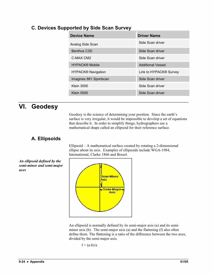
A. Ellipsoids Ellipsoid – A mathematical surface created by rotating a 2-dimensional ellipse about its axis. Examples of ellipsoids include WGA-1984, International, Clarke 1866 and Bessel.
An ellipsoid defined by the semi-minor and semi-major axes
An ellipsoid is normally defined by its semi-major axis (a) and its semi-minor axis (b). The semi-major axis (a) and the flattening (f) also often define them. The flattening is a ratio of the difference between the two axes, divided by the semi-major axis.
f = (a-b)/a
1/05 Appendix •••• 9-25
The semi-major and semi-minor axes are normally expressed in meters. The flattening is often expressed as the inverse (1/f) of the flattening.
Sample values for some common ellipsoids are: Ellipsoid a (m) b (m) 1/f
Bessel 6,378,206.4 299.1528128
Clarke 1866 6378206.4 294.9784982
Clarke 1880 6378249.145 293.465
GRS 1980 6378137.0 298.25722101
Everest 6377276.345 300.8017
International 6378388.0 298.0
WGS 1972 6378135.0 298.26
WGS 1984 6378137. 298.257223563
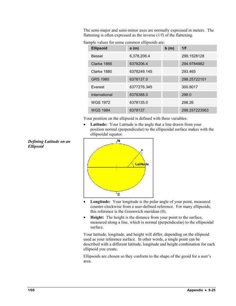
Your position on the ellipsoid is defined with three variables: • Latitude: Your Latitude is the angle that a line drawn from your
position normal (perpendicular) to the ellipsoidal surface makes with the ellipsoidal equator.
Defining Latitude on an Ellipsoid
• Longitude: Your longitude is the polar angle of your point, measured
counter-clockwise from a user-defined reference. For many ellipsoids, this reference is the Greenwich meridian (0).
• Height: The height is the distance from your point to the surface, measured along a line, which is normal (perpendicular) to the ellipsoidal surface.
Your latitude, longitude, and height will differ, depending on the ellipsoid used as your reference surface. In other words, a single point can be described with a different latitude, longitude and height combination for each ellipsoid you create.
Ellipsoids are chosen so they conform to the shape of the geoid for a user’s area.

9-26 •••• Appendix 01/05
B. Geoids A geoid is an equipotential surface, meaning the pull of gravity measured anywhere on the surface is equal. Base on the surrounding mass (mountains, canyons, etc.), this surface rises and falls and is much more irregular than an ellipsoid, although much smoother than the earth’s surface.
One of the important features about a geoid is that a plumb bob always points normal (perpendicular) to the geoidal surface. It does not point directly to the center of the earth. This means that your local land measurements will be affected by the local geoidal surface. In order to reduce the errors caused in computing positions on the ellipsoid using measurements affected by the geoid, the ellipsoid is shifted so it closely matches the geoid in your local area. When this is done, it becomes a datum.
C. Datums A datum is an ellipsoidal surface, which has been moved to closely match the geoidal surface for a user’s area. Examples of datums include NAD1927 (using the Clarke 1880 ellipsoid), NAD1983 (using the GRS-1980 ellipsoid) and Bogota Datum (using the International ellipsoid).
When you move your ellipsoid to create a datum, you are also affecting the latitude, longitude and height above the ellipsoid of your point. When someone describes a position location to you with latitude, longitude and height, you don’t know anything until you know which datum was used to define the point and which ellipsoid the datum is based upon.
Example #1: Say that your friend confesses to you on his deathbed that he robbed a bank and buried the money at exactly 45N and 78W. You had better quickly ask him what his reference datum was, or you are going to be digging a long time!
Example #2: An oil company pays you a lot of money to survey between 26 00N and 72 00W and 26 01N and 72 01W. Since they are a modern survey company, you assume they are working on WGS-84 and go out and perform the survey. When you get back home, you find out they are working on the Everest ellipsoid and you should have been surveying an area 2 miles to the south.
D. Datum Transformations There is always a need to be able to convert a latitude, longitude and height from one datum to another. This is performed with a datum transformation.
For example, your DGPS provides you with a position in WGS-84. Your survey is being performed on NAD1927. In order to convert the position from WGS-84 to NAD1927, you need to perform the datum transformation.
Datum transformations can be performed using several different methods. Among them are the geocentric, regression formulae, exact, and numerical difference techniques.
1/05 Appendix •••• 9-27
1) Three-Parameter Datum Transformation In geocentric methods, the latitude, longitude and height above the ellipsoid are converted to Cartesian XYZ coordinates using the center of the ellipsoid as the origin. These are referred to as “geocentric coordinates”. Based upon the separation between the centers of the two datums, an offset is added to each coordinate to “shift” them from the first datum to the second datum. The geocentric coordinates for the second datum are then converted back into latitude, longitude and height using the ellipsoidal constants for the second ellipsoid.
In summary:
Lat1/Long1/H1 X1, Y1, Z1, X2,Y2,Z2 Lat2/Long2/H2
To go from X1, Y1, Z1 to X2, Y2, Z2, we added a dX, dY and dZ to each specific value. This is called a three-parameter shift and is typically used for only a local area (10km). The same process is performed in a technique known as the Molodensky Formulae. The Abridged Molodensky Formulae is very similar, but eliminates a few variables while giving almost the same result.
To obtain these dX, dY and dZ values, users can either look up published information (such as DMA TM 8511) or calculate them. To calculate them, you need to know the latitude, longitude and height for the same point in the two different datums. Calculate the geocentric coordinates for both points, using the ellipsoidal parameters associated with each datum. Take the difference between the X1 and X2 values to determine the dX parameter. Repeat the same for the dY and dZ parameters. Voila, you have computed the exact datum transformation parameters for your area.
The dX, dY, and dZ values used in a datum transformation are typically valid for a small area (10 km X 10km?). As you move further from your area, the values change as the relationship between the two ellipsoids change.
2) Seven-Parameter Datum Transformation To cover a wider area, a seven-parameter datum transformation can be used. A seven-parameter transformation contains, the dX, dY and dZ values mentioned above, as well as ӨX, ӨY and ӨZ and dScale values. The Ө values represent the difference in alignment of the X-, Y-, and Z-axis of the two ellipsoidal geocentric axes. The dScale represents difference in scale measured between the two systems.
The advantage of a seven-parameter datum transformation over a three-parameter datum transformation is that it is valid for a much larger area. Many countries, such a Saudi Arabia publish a single seven-parameter datum transform, which is used for the entire country.
3) Regression Formulae Regression Formulae are also used to convert between specific datums. The transformation is achieved by using the latitude, longitude and height above ellipsoid on the output datum.
9-28 •••• Appendix 01/05
Although quite handy for computer programs, regression formulae are not widely implemented. A main problem is you must have a separate regression equation for each set of datums you wish to transform between. An additional problem is that regression equation coefficients are computed using actual data sets. If you have sparse data, your results may not be accurate away from your data points. Regression equations also tend to “smooth” through local abnormalities.
4) Exact Formulae The relationship between certain datums can be described by exact formulae. One of the primary examples of exact formulae is the conversion between WGS-1972 and WGS-1984.
5) Numerical Difference Technique Another method for datum conversion is the numerical difference technique. A primary example of this technique is the DANCON transformation routine used throughout the U.S. Army Corps of Engineers (USACE). Using a huge set of test points, USACE developed a gridded model of the difference between NAD 1927 and WGS-84 latitude/longitude/heights. Based on a users position, NADCON determines the surrounding difference in latitude/longitude/height for the four corners of the grid cell containing your position and then interpolates the dLat, dLong and dHeight for your point. Although limited for use between WGS-84 and NAD-27, NADCON serves as the datum transformation engine for the CORPSCON program that has a large group of users.
E. Projections A projection is a flat (2-dimensional) representation of a 3-dimensional surface.
In order to present hydrographic data on flat, easy-to-store charts, hydrographers have always been faced with the challenge of accurately representing the real world in two dimensions. To accomplish this task, a projection is used. The key to choosing a good projection is to minimize the amount of distortion that takes place when moving between the real world and the flat chart.
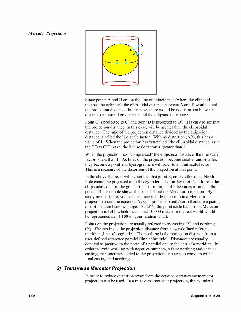
1) Mercator Projection Most projections are based upon either cylindrical or conical shapes. In the figure to the right, the ellipsoid has been wrapped by a giant cylinder that “touches” the ellipsoid at the equator. If there was a light source at the center of the ellipsoid, all points on the ellipsoidal surface could be projected somewhere on the cylinder. For example, point D on the ellipsoid in the figure below would be projected to D1 on the cylindrical projection.
1/05 Appendix •••• 9-29
Mercator Projections
Since points A and B are on the line of coincidence (where the ellipsoid touches the cylinder), the ellipsoidal distance between A and B would equal the projection distance. In this case, there would be no distortion between distances measured on our map and the ellipsoidal distance.
Point C is projected to C1 and point D is projected to D1. It is easy to see that the projection distance, in this case, will be greater than the ellipsoidal distance. The ratio of the projection distance divided by the ellipsoidal distance is called the line scale factor. With no distortion (AB), this has a value of 1. When the projection has “stretched” the ellipsoidal distance, as in the CD to C1D1 case, the line scale factor is greater than 1.
When the projection has “compressed” the ellipsoidal distance, the line scale factor is less than 1. As lines on the projection become smaller and smaller, they become a point and hydrographers will refer to a point scale factor. This is a measure of the distortion of the projection at that point.
In the above figure, it will be noticed that point E, on the ellipsoidal North Pole cannot be projected onto this cylinder. The further north/south from the ellipsoidal equator, the greater the distortion, until it becomes infinite at the poles. This example shows the basis behind the Mercator projection. By studying the figure, you can see there is little distortion in a Mercator projection about the equator. As you go further south/north from the equator, distortion soon becomes large. At 45oN, the point scale factor on a Mercator projection is 1.41, which means that 10,000 meters in the real world would be represented as 14,100 on your nautical chart.
Points on the projection are usually referred to by easting (X) and northing (Y). The easting is the projection distance from a user-defined reference meridian (line of longitude). The northing is the projection distance from a user-defined reference parallel (line of latitude). Distances are usually denoted as positive to the north of a parallel and to the east of a meridian. In order to avoid working with negative numbers, a false northing and/or false easting are sometimes added to the projection distances to come up with a final easting and northing.
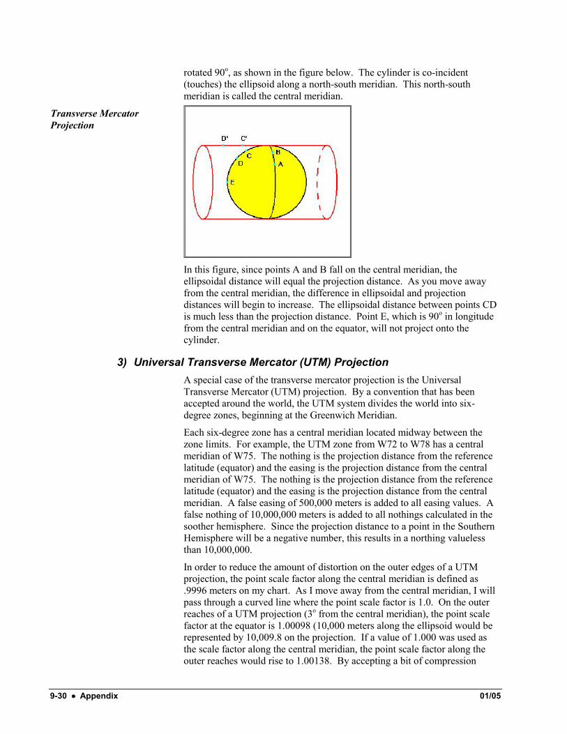
2) Transverse Mercator Projection In order to reduce distortion away from the equator, a transverse mercator projection can be used. In a transverse mercator projection, the cylinder is
9-30 •••• Appendix 01/05
rotated 90o, as shown in the figure below. The cylinder is co-incident (touches) the ellipsoid along a north-south meridian. This north-south meridian is called the central meridian.
Transverse Mercator Projection
In this figure, since points A and B fall on the central meridian, the ellipsoidal distance will equal the projection distance. As you move away from the central meridian, the difference in ellipsoidal and projection distances will begin to increase. The ellipsoidal distance between points CD is much less than the projection distance. Point E, which is 90o in longitude from the central meridian and on the equator, will not project onto the cylinder.
3) Universal Transverse Mercator (UTM) Projection A special case of the transverse mercator projection is the Universal Transverse Mercator (UTM) projection. By a convention that has been accepted around the world, the UTM system divides the world into six-degree zones, beginning at the Greenwich Meridian.
Each six-degree zone has a central meridian located midway between the zone limits. For example, the UTM zone from W72 to W78 has a central meridian of W75. The nothing is the projection distance from the reference latitude (equator) and the easing is the projection distance from the central meridian of W75. The nothing is the projection distance from the reference latitude (equator) and the easing is the projection distance from the central meridian. A false easing of 500,000 meters is added to all easing values. A false nothing of 10,000,000 meters is added to all nothings calculated in the soother hemisphere. Since the projection distance to a point in the Southern Hemisphere will be a negative number, this results in a northing valueless than 10,000,000.
In order to reduce the amount of distortion on the outer edges of a UTM projection, the point scale factor along the central meridian is defined as .9996 meters on my chart. As I move away from the central meridian, I will pass through a curved line where the point scale factor is 1.0. On the outer reaches of a UTM projection (3o from the central meridian), the point scale factor at the equator is 1.00098 (10,000 meters along the ellipsoid would be represented by 10,009.8 on the projection. If a value of 1.000 was used as the scale factor along the central meridian, the point scale factor along the outer reaches would rise to 1.00138. By accepting a bit of compression
1/05 Appendix •••• 9-31
along the central meridian, we have reduced the amount of stretching needed at the outer limits of the projection. UTM projections are used from 80oN to 80oS. Although there is no distortion along the central meridian in the polar regions, the distortion begins to become unacceptably large as you move to the edge of the zone.
Some countries, such as Canada, use a modified UTM system. In Canada, the zones span only 3o of longitude.
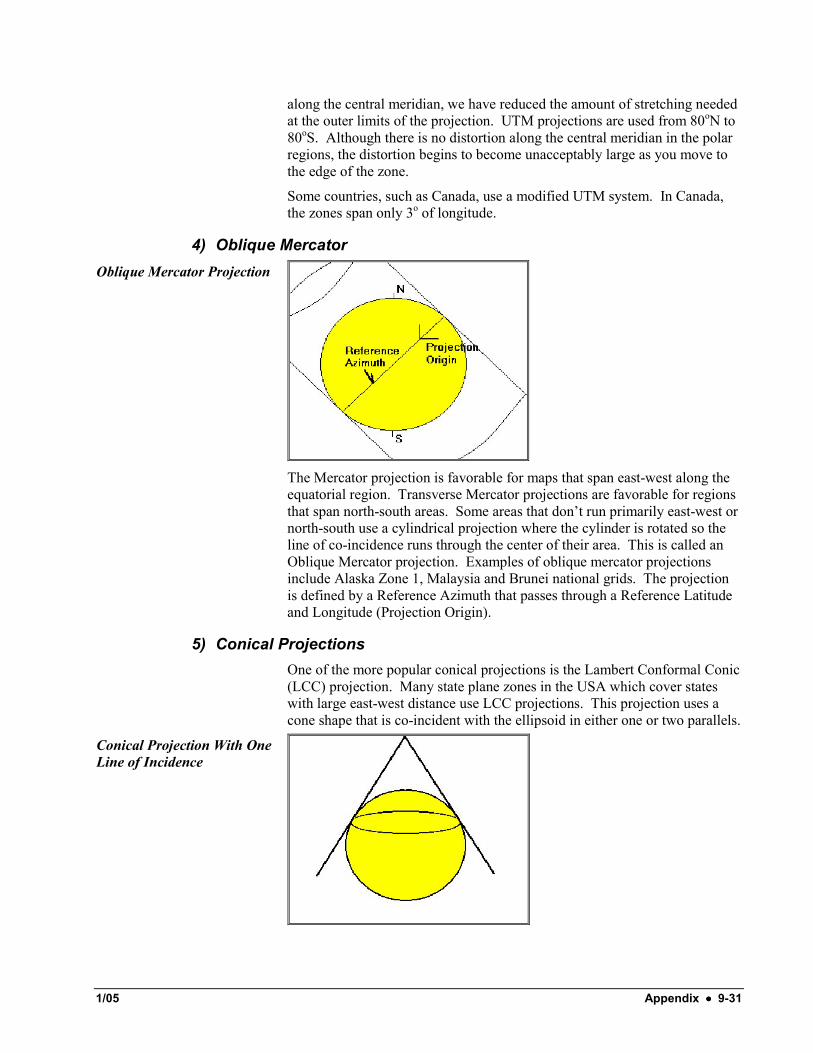
4) Oblique Mercator Oblique Mercator Projection
The Mercator projection is favorable for maps that span east-west along the equatorial region. Transverse Mercator projections are favorable for regions that span north-south areas. Some areas that don’t run primarily east-west or north-south use a cylindrical projection where the cylinder is rotated so the line of co-incidence runs through the center of their area. This is called an Oblique Mercator projection. Examples of oblique mercator projections include Alaska Zone 1, Malaysia and Brunei national grids. The projection is defined by a Reference Azimuth that passes through a Reference Latitude and Longitude (Projection Origin).
5) Conical Projections One of the more popular conical projections is the Lambert Conformal Conic (LCC) projection. Many state plane zones in the USA which cover states with large east-west distance use LCC projections. This projection uses a cone shape that is co-incident with the ellipsoid in either one or two parallels.
Conical Projection With One Line of Incidence
9-32 •••• Appendix 01/05
The projection is normally defined with either a single or two parallels (north and south). Northings are measured from a reference latitude and eastings are measured from a central meridian.
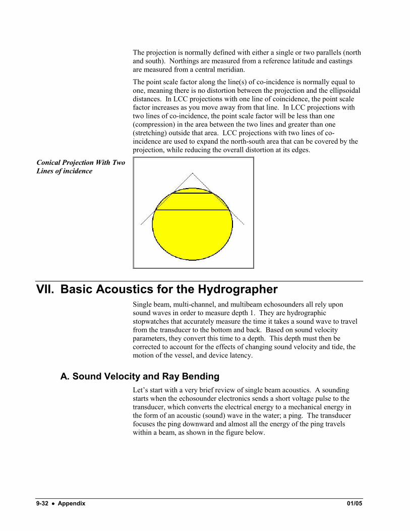
The point scale factor along the line(s) of co-incidence is normally equal to one, meaning there is no distortion between the projection and the ellipsoidal distances. In LCC projections with one line of coincidence, the point scale factor increases as you move away from that line. In LCC projections with two lines of co-incidence, the point scale factor will be less than one (compression) in the area between the two lines and greater than one (stretching) outside that area. LCC projections with two lines of co-incidence are used to expand the north-south area that can be covered by the projection, while reducing the overall distortion at its edges.
Conical Projection With Two Lines of incidence
VII. Basic Acoustics for the Hydrographer Single beam, multi-channel, and multibeam echosounders all rely upon sound waves in order to measure depth 1. They are hydrographic stopwatches that accurately measure the time it takes a sound wave to travel from the transducer to the bottom and back. Based on sound velocity parameters, they convert this time to a depth. This depth must then be corrected to account for the effects of changing sound velocity and tide, the motion of the vessel, and device latency.
A. Sound Velocity and Ray Bending Let’s start with a very brief review of single beam acoustics. A sounding starts when the echosounder electronics sends a short voltage pulse to the transducer, which converts the electrical energy to a mechanical energy in the form of an acoustic (sound) wave in the water; a ping. The transducer focuses the ping downward and almost all the energy of the ping travels within a beam, as shown in the figure below.

1/05 Appendix •••• 9-33
Single Beam Sounding Through sound velocity Change. No change in the beam direction occurs.
The ping travels at the speed of sound in water. Where the sound velocity changes due to temperature or density variations, like at the boundary between velocities 1 and 2, the ping speed changes. A very small portion of the energy is reflected back upward, but the ping still travels straight down; there is no change in direction.
When the ping reaches the bottom, it encounters a large change in velocity (V3). This is because sound travels much faster in the solid bottom than it does in a liquid. A large amount of the ping energy is reflected (echoed) upward at this transition and eventually finds its way back to the transducer. The transducer converts the reflected sound back to the electrical energy. From the time delay between the outgoing and incoming pulses (and known acoustic velocity in water), depth is calculated.
Now, we take a look at multibeam sonar. In multibeam technology, a beam is sometimes called a ray, which is a mathematical term for a line with a direction. In the single beam case above, it is two directions, first down then up.
Multibeam sounding through sound velocity change; the beam is refracted upward. (V2 is greater than V1)
With multibeam, the beams are not necessarily vertical, and that changes the situation. When a non-vertical beam encounters a change in sound velocity, not only does the ping change speed, the beam (ray) changes direction slightly. This effect is known as refraction or ray bending. When sound velocity increases (v2 > v1), the ray is bent upward. Conversely, when the sound velocity decreases (v1>v2), the ray is bent downward. Snell’s Law gives the magnitude of refraction.
V1/Sin(theta 1) = V2/Sin(theta 2) where theta 1 and 2 are the vertical ray angles in V1 and V2 respectively.
In the following figure, two examples are illustrated. A single beam system pointed directly below the boat and a beam from a multiple transducer
9-34 •••• Appendix 01/05
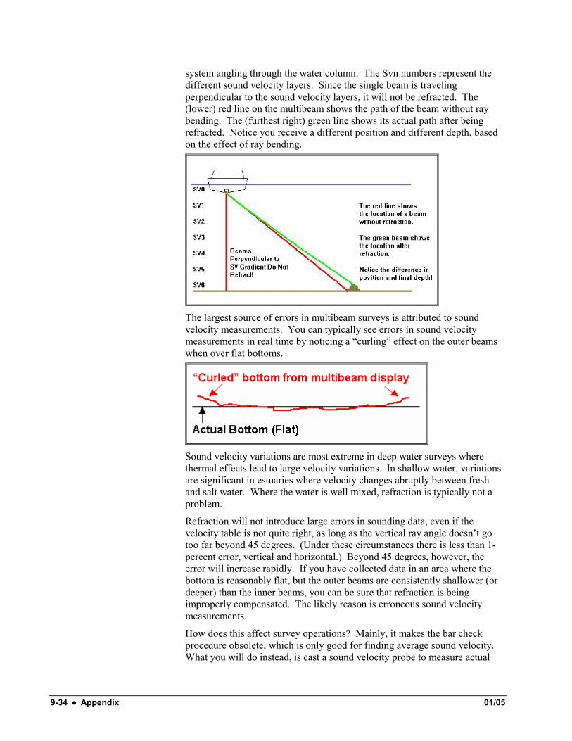
system angling through the water column. The Svn numbers represent the different sound velocity layers. Since the single beam is traveling perpendicular to the sound velocity layers, it will not be refracted. The (lower) red line on the multibeam shows the path of the beam without ray bending. The (furthest right) green line shows its actual path after being refracted. Notice you receive a different position and different depth, based on the effect of ray bending.
The largest source of errors in multibeam surveys is attributed to sound velocity measurements. You can typically see errors in sound velocity measurements in real time by noticing a “curling” effect on the outer beams when over flat bottoms.
Sound velocity variations are most extreme in deep water surveys where thermal effects lead to large velocity variations. In shallow water, variations are significant in estuaries where velocity changes abruptly between fresh and salt water. Where the water is well mixed, refraction is typically not a problem.
Refraction will not introduce large errors in sounding data, even if the velocity table is not quite right, as long as the vertical ray angle doesn’t go too far beyond 45 degrees. (Under these circumstances there is less than 1- percent error, vertical and horizontal.) Beyond 45 degrees, however, the error will increase rapidly. If you have collected data in an area where the bottom is reasonably flat, but the outer beams are consistently shallower (or deeper) than the inner beams, you can be sure that refraction is being improperly compensated. The likely reason is erroneous sound velocity measurements.
How does this affect survey operations? Mainly, it makes the bar check procedure obsolete, which is only good for finding average sound velocity. What you will do instead, is cast a sound velocity probe to measure actual

1/05 Appendix •••• 9-35
velocity variations with depth. The Velocity vs. Depth information is entered into a table that is used during post-processing to compensate for refraction.
B. Beam Frequency Effects on Survey Data As the frequency of your EM wave increases, so does the precision of your measurement. Put hydrographers’ terms, the higher the frequency of your transducer, the more accurate your measurement will be. High-resolution side scan sonars use frequencies of 500KHZ. Multibeam systems for small launches use frequencies from 200KHZ to 450KHZ. Traditional single beam echosounder use frequencies around 200MHZ. Some hydrographers (for reasons to be discussed) use transducers with 24KHZ to 33KHZ. After reading this, you think everybody would be using 500KHZ transducers, but there is a price to pay for precision.
The higher the frequency of the EM wave, the greater the energy dissipation. As sound waves travel through water, their energy is dissipated by particles in the water, air bubbles, etc. High frequency sound waves quickly dissipate and cannot be used in deeper water. Deep-water transducers, used to measure depths of greater than 1000 meters, are typically in the range from 3KHZ to 12KHZ. Although not as precise as 200KHZ transducers, they can produce sound waves that can get to the bottom and back without dissipating.
The higher the frequency, the higher the reflectivity. One of the drawbacks with higher frequency (200+KHZ) transducers is they reflect off almost anything. This includes vegetation, air bubbles, fish bladders, and suspended sediments. A lower frequency transducer (e.g. 24KHZ), although slightly less precise, will allow you to pass through some of these materials to actually track the bottom. Over a soft mud, sand, silt) bottom, a low frequency transducer will generally provide deeper depths than a high frequency transducer. Over a hard (rock) bottom, the two transducers should produce almost the same depth.
The lower the frequency, the larger the transducer. The physical size of transducers has certainly been reduced over the last decades. However, this rule generally still holds true. Lower frequency transducers are heavier and larger than higher frequency transducers and sometimes can complicate the mounting procedures.
C. Beam Geometry The equipment required for a single beam survey is a positioning system, an echosounder and, if the water is choppy, a heave compensator. Mount the position antenna above the transducer, and the sounding x and y are the same as antenna x and y. Depth (z) is the sounding minus heave. It's simple.
For accurate multibeam surveying, you need some additional equipment: a gyro to measure boat heading and a MRU (motion reference unit) for the pitch and roll data. The reason for the additional measurements is, again, because the directed beams are not vertical so calculation of the sounding x, y, and z values becomes more complex than in single beam surveys.
9-36 •••• Appendix 01/05
Note: MRU and Heave Compensator are interchangeable terms, although MRU more accurately describes what these things do.
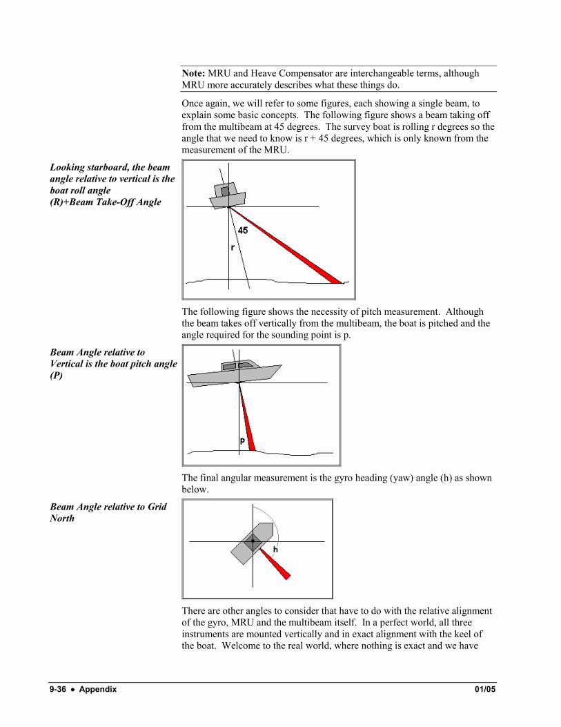
Once again, we will refer to some figures, each showing a single beam, to explain some basic concepts. The following figure shows a beam taking off from the multibeam at 45 degrees. The survey boat is rolling r degrees so the angle that we need to know is r + 45 degrees, which is only known from the measurement of the MRU.
Looking starboard, the beam angle relative to vertical is the boat roll angle (R)+Beam Take-Off Angle
The following figure shows the necessity of pitch measurement. Although the beam takes off vertically from the multibeam, the boat is pitched and the angle required for the sounding point is p.
Beam Angle relative to Vertical is the boat pitch angle (P)
The final angular measurement is the gyro heading (yaw) angle (h) as shown below.
Beam Angle relative to Grid North
There are other angles to consider that have to do with the relative alignment of the gyro, MRU and the multibeam itself. In a perfect world, all three instruments are mounted vertically and in exact alignment with the keel of the boat. Welcome to the real world, where nothing is exact and we have
1/05 Appendix •••• 9-37
magnetic variations and mounting offset angles to accommodate. These offset angles must be added to the beam roll, pitch and heading angles. Note that it is nearly impossible to measure these angles accurately enough for survey quality data. That’s why the Patch Test is done -- to let the computer figure out the angles for you.
Solving for sounding x, y, z requires a few steps, and is outside the scope of this introductory course. It’s enough to say, the equations are ugly, but they work!
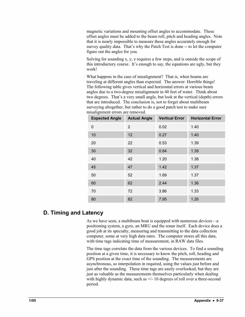
What happens in the case of misalignment? That is, when beams are traveling at different angles than expected. The answer: Horrible things! The following table gives vertical and horizontal errors at various beam angles due to a two-degree misalignment in 40 feet of water. Think about two degrees. That’s a very small angle, but look at the vertical (depth) errors that are introduced. The conclusion is, not to forget about multibeam surveying altogether, but rather to do a good patch test to make sure misalignment errors are removed.
Expected Angle Actual Angle Vertical Error Horizontal Error
0 2 0.02 1.40
10 12 0.27 1.40
20 22 0.53 1.39
30 32 0.84 1.39
40 42 1.20 1.38
45 47 1.42 1.37
50 52 1.69 1.37
60 62 2.44 1.36
70 72 3.86 1.33
80 82 7.95 1.26
D. Timing and Latency As we have seen, a multibeam boat is equipped with numerous devices—a positioning system, a gyro, an MRU and the sonar itself. Each device does a good job at its specialty, measuring and transmitting to the data collection computer, some at very high data rates. The computer stores all this data, with time tags indicating time of measurement, in RAW data files.
The time tags correlate the data from the various devices. To find a sounding position at a given time, it is necessary to know the pitch, roll, heading and GPS position at the exact time of the sounding. The measurements are asynchronous, so interpolation in required, using the values just before and just after the sounding. These time tags are easily overlooked, but they are just as valuable as the measurements themselves particularly when dealing with highly dynamic data, such as +/- 10 degrees of roll over a three-second period.
9-38 •••• Appendix 01/05
Admittedly, there isn’t much you can do about system timing except (1) to sample devices often and (2) account for device latency.
1) Update Frequency The more frequently devices are sampled, the better. It is far preferable to have too much data than not enough. In HYPACK® MAX, this means setting the update frequency to the maximum value of 50 milliseconds for all devices.
2) Latency Latency is a device parameter that gives the time delay between measurement and transmission to the data collection computer. Some devices measure, then spend time processing or waiting for additional input, then transmit after a delay; these devices have latency. Some devices measure then transmit after an insignificant time delay, in which case the latency time is zero. Other devices have predictive filters that predict the value at time of transmission, and therefore have zero latency also. Some devices transmit after a delay, but include latency in the transmission.
Latency is subtracted for the time tag to give time of measurement. When latency is wrong, the time tag is wrong and the correlation between devices is wrong so the data is wrong. It is clear that you must know latency values either from the device manual or Tech. Support, a patch test (for positioning systems) or HYPACK, Inc..
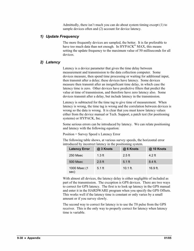
Some serious errors can be introduced by latency. We can relate positioning and latency with the following equation:
Position = Survey Speed x Latency Error
The following table shows, at various survey speeds, the horizontal error introduced by incorrect latency in the positioning system.
Latency Error @ 3 Knots @ 6 Knots @ 10 Knots
250 Msec 1.3 ft 2.5 ft 4.2 ft
500 Msec 2.5 ft 5.1 ft 8.4 ft.
1000 Msec (1 sec)
5.1 ft 10.1 ft. 16.9 ft.
With almost all devices, the latency delay is either negligible of included as part of the transmission. The exception is GPS devices. There are two ways to correct for GPS latency. The first is to look up latency in the GPS manual and enter it in the HARDWARE program when you specify the GPS Offsets. This works well if the latency time is constant or only varies by a small amount or if you survey slowly.
The second way to correct for latency is to use the T0 pulse from the GPS receiver. This is the only way to properly correct for latency when latency time is variable.
1/05 Appendix •••• 9-39
Update frequency is how often the SURVEY program checks for device data. Use 50 milliseconds for all devices with one exception. If you are surveying in calm water, you can reduce the size of your data files by decreasing the MRU update frequency. You will have to experiment to find a value that reduces files size while providing acceptable data quality.
VIII. Echosounders 101
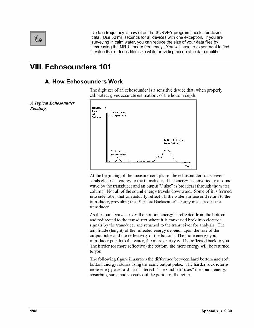
A. How Echosounders Work The digitizer of an echosounder is a sensitive device that, when properly calibrated, gives accurate estimations of the bottom depth.
A Typical Echosounder Reading
At the beginning of the measurement phase, the echosounder transceiver sends electrical energy to the transducer. This energy is converted to a sound wave by the transducer and an output "Pulse” is broadcast through the water column. Not all of the sound energy travels downward. Some of it is formed into side lobes that can actually reflect off the water surface and return to the transducer, providing the “Surface Backscatter” energy measured at the transducer.
As the sound wave strikes the bottom, energy is reflected from the bottom and redirected to the transducer where it is converted back into electrical signals by the transducer and returned to the transceiver for analysis. The amplitude (height) of the reflected energy depends upon the size of the output pulse and the reflectivity of the bottom. The more energy your transducer puts into the water, the more energy will be reflected back to you. The harder (or more reflective) the bottom, the more energy will be returned to you.
The following figure illustrates the difference between hard bottom and soft bottom energy returns using the same output pulse. The harder rock returns more energy over a shorter interval. The sand “diffuses” the sound energy, absorbing some and spreads out the period of the return.

9-40 •••• Appendix 01/05
Comparing Echosounder readings over different Bottom materials
Most electronic digitizers on echosounders use a “Threshold” or “Sensitivity” setting to determine the energy level of the return signal that represents the bottom. Examine the following diagram. The Threshold is set at the “T1” level. This results in a measurement shown as “Depth 1”. If we raise the threshold to the “T2” level, the depth will increase to “Depth 2”. We can influence the depth by adjusting the digitizer threshold. In the "Rock/Sand” example, it can also be seen that we will receive slightly different depths over different material using the same digitizer threshold.
Beware ! If you calibrate your echosounder over hard rock and then conduct your survey over a sandy bottom, you can introduce errors into your depth measurement!
The Influence of Digitizer Threshold on Depth Readings
We can also influence the depth by controlling the amplitude of the output pulse. Examine the figure below. With the echosounder outputting power in the black (Depth 1) setting, the digitizer analyzes the return data and sets the depth where the reflected energy is greater than the Digitizer Threshold at “Depth 1”. We then increase the output power to the red (Depth 2) setting. The reflected energy also increases in amplitude and it exceeds the Digitizer Threshold slightly earlier. This results in the echosounder outputting “Depth 2”. As you increase the output power on your echosounder, you can
1/05 Appendix •••• 9-41
potentially decrease the measured depth. The inverse of this is also true. Decreasing the output power can result in increased depth measurements.
Comparing Echosounder Readings at Different output powers
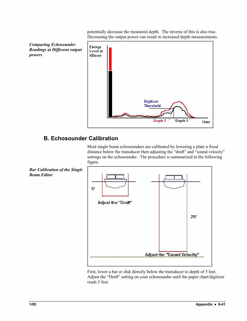
B. Echosounder Calibration Most single beam echosounders are calibrated by lowering a plate a fixed distance below the transducer then adjusting the “draft” and “sound velocity” settings on the echosounder. The procedure is summarized in the following figure.
Bar Calibration of the Single Beam Editor
First, lower a bar or disk directly below the transducer to depth of 5 feet. Adjust the “Draft” setting on your echosounder until the paper chart/digitizer reads 5 feet.

9-42 •••• Appendix 01/05
Next, lower the bar/disk to a depth that is approximately the depth of your channel. In our example, we have lowered it to 25 feet. Adjust the “Sound Velocity” setting until your echosounder reads 25 feet.
Now return the bar/disk to 5 feet and check the depth. It may have changed, since you just changed the sound velocity. If it has not changed, your echosounder is calibrated and you may begin work. If it has changed, use the draft setting to return it to five feet. Lower the bar/disk once again to 25 feet and check the sound velocity. You will have to adjust it to read 25 feet. Return once again to 5 feet to check.
Repeat this process until the sounder accurately reports the 5-foot and 25 foot levels.
Using this process, you now have an echosounder that is calibrated at 5 feet and 25 feet. Assuming the sound velocity is constant through the water column, it should also be calibrated for the depths between this range. If sound velocity is not a constant through these ranges, your intermediate depths may have small errors.
Slight depth errors occurring due to sound velocity factors
Another method used for calibrating your echosounder is to set the sounder for a fixed velocity (for example 1500m/s or 4800 ft/s) and then use a sound velocity profile to adjust the depths in real time or post processing. The sounder is first calibrated using the process described above. This finds the electronic draft of the sounder. After calibration, the velocity is then set at a recommended level. Measured depths are later adjusted based on the initial setting and the sound velocity profile to determine the final measured depth.
C. Beam Patterns Based on the transducer design, echosounders produce different shaped beams. Some beams are narrow; some are wide. Most transducers have a beam pattern that shows the energy levels at various angles and signal strengths (dB levels). Most echosounders used in hydrographic surveying have a main beam that is directed perpendicular from the transducer ace plate. Two “side lobes” form at angles from the main beam. The typical pattern of a transducer beam pattern is shown in the figure below.

1/05 Appendix •••• 9-43
Transducer Beam Angle
The “beam angle” of a transducer is determined by measuring the range of the 6dB level. In this example, the transducer would have a beam angle of 8 degrees.
IX. Launching External Programs from the HYPACK® MAX Menu
You can use the TOOLS menu that will launch external executable files. Just another handy alternative to using the usual Windows® methods.
1. Select TOOLS-SETUP. The Tool Options dialog will appear.
Tool Options dialog
2. Click [Add] and the Tool Options Properties dialog will appear.
Tool Options Properties dialog
3. Fill in the fields of the dialog then click [OK] and close the program.
The contents of the Title field will now appear in the HYPACK® MAX Help menu. In the future, when you select this menu item, it will launch the Program named in the second field and pass it any Parameters that you have listed.

9-44 •••• Appendix 01/05
The Current Project checkbox (not pictured here) is for internal use at HYPACK, Inc. only.
You can add as many programs as you want in this manner and use the up and down arrow buttons to arrange their order if desired.
To remove programs from the menu:
Open the Tool Options dialog, select the program to be removed and click [Delete].
To change the properties of any listed program:
Open the Tool Options dialog, select the program then click [Edit]. The Tool Options Properties dialog will appear with the current data and you can edit it as desired.