alicia m. sintes universitat de les illes balears pisa,1 june 2007 data analysis searches for...
TRANSCRIPT
Alicia M. Sintes Universitat de les Illes Balears
Pisa,1 June 2007
Data analysis searches for continuous gravitational waves
VESF-school, Pisa, June 2007, A.M. Sintes 2
Content
• Gravitational waves from spinning neutron stars.– Emission mechanisms– Signal model
• Data analysis for continuous gravitational waves– Bayesian analysis– Frequentist approach
• Brief overview of the searches – Directed pulsar search– Wide-parameter search (all sky)
• Coherent methods• Einstein@Home• Hierarchical strategies• Semi-coherent methods
• Summary of results and perspectives
VESF-school, Pisa, June 2007, A.M. Sintes 3
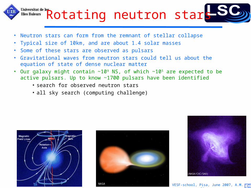
Rotating neutron stars
(NASA/CXC/SAO)
NASA
• Neutron stars can form from the remnant of stellar collapse
• Typical size of 10km, and are about 1.4 solar masses
• Some of these stars are observed as pulsars
• Gravitational waves from neutron stars could tell us about the equation of state of dense nuclear matter
• Our galaxy might contain ~109 NS, of which ~105 are expected to be active pulsars. Up to know ~1700 pulsars have been identified
• search for observed neutron stars
• all sky search (computing challenge)
VESF-school, Pisa, June 2007, A.M. Sintes 4
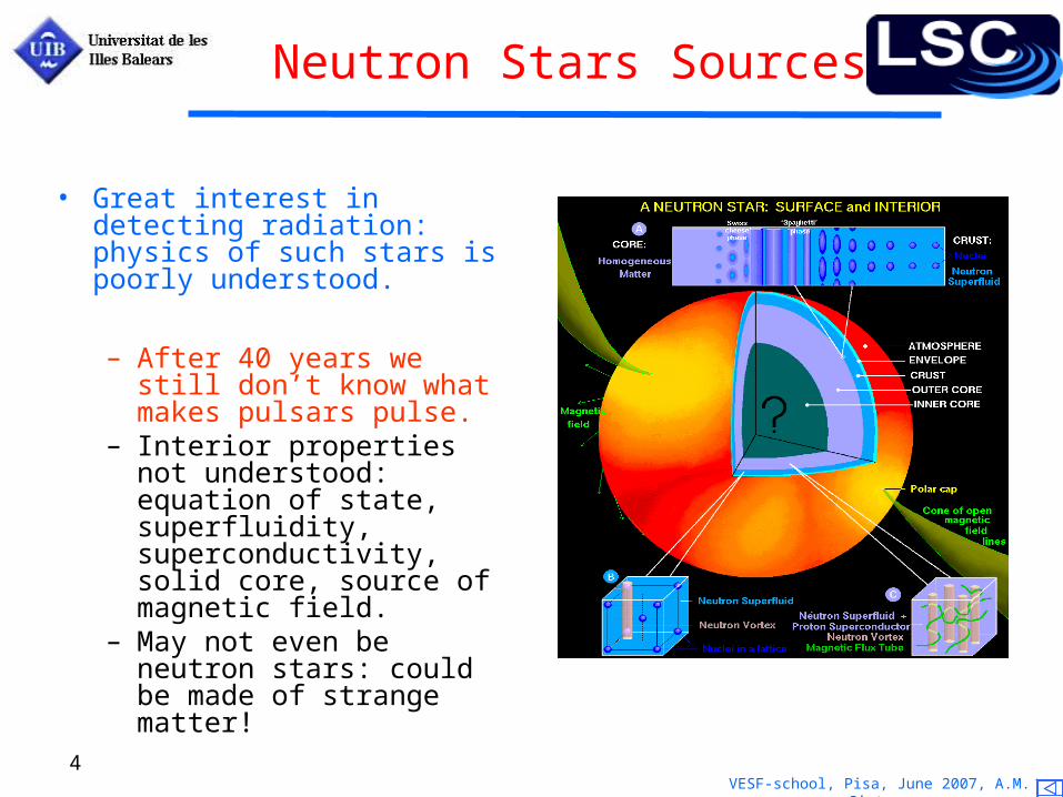
Neutron Stars Sources
• Great interest in detecting radiation: physics of such stars is poorly understood.
– After 40 years we still don’t know what makes pulsars pulse.
– Interior properties not understood: equation of state, superfluidity, superconductivity, solid core, source of magnetic field.
– May not even be neutron stars: could be made of strange matter!
VESF-school, Pisa, June 2007, A.M. Sintes 5
“Continuous” gravitational waves from neutron stars
Various physical mechanisms could operate in a NS to produce interesting levels of GW emission
As the signal-strength is generally expected to be weak, long integrations times (several days to years) are required in order for the signal to be
detectable in the noise.
Therefore this GW emission has to last for a long time, which characterizes the class of ‘continuous-wave’ signals.
NS might also be interesting sources of burst-like GW emission, f-mode or p-mode oscillations excited by a glitch
crustal torsion modes
QuickTime™ and aTIFF (Uncompressed) decompressor
are needed to see this picture.
VESF-school, Pisa, June 2007, A.M. Sintes 6
Bumpy Neutron Star
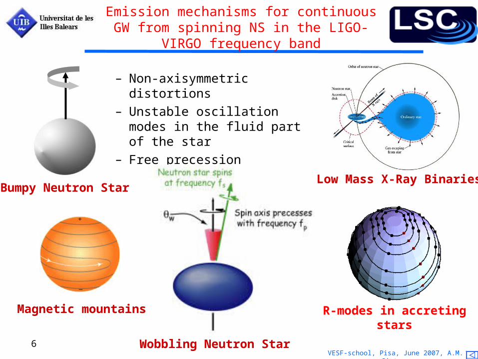
Emission mechanisms for continuous GW from spinning NS in the LIGO-VIRGO frequency band
– Non-axisymmetric distortions
– Unstable oscillation modes in the fluid part of the star
– Free precession
Wobbling Neutron Star
Low Mass X-Ray Binaries
Magnetic mountains R-modes in accreting stars
VESF-school, Pisa, June 2007, A.M. Sintes 7
Bumpy Neutron Star
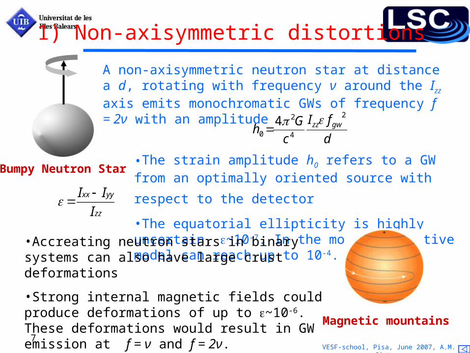
1) Non-axisymmetric distortions
A non-axisymmetric neutron star at distance a d, rotating with frequency ν around the Izz axis emits monochromatic GWs of frequency f = 2ν with an amplitude
h0 4 2G
c 4
Izz fgw2
d
Ixx Iyy
Izz
•The strain amplitude h0 refers to a GW from an optimally
oriented source with respect to the detector •The equatorial ellipticity is highly uncertain, ~10-7. In the most speculative model can reach up to 10-4.
•Accreating neutron stars in binary systems can also have large crust deformations
•Strong internal magnetic fields could produce deformations of up to ~10-6. These deformations would result in GW emission at f = ν and f = 2ν.
Magnetic mountains
VESF-school, Pisa, June 2007, A.M. Sintes 8Wobbling Neutron Star
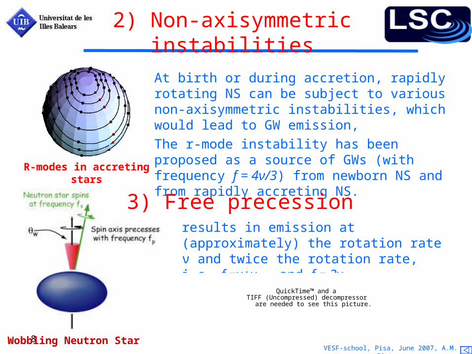
2) Non-axisymmetric instabilities
At birth or during accretion, rapidly rotating NS can be subject to various non-axisymmetric instabilities, which would lead to GW emission,
The r-mode instability has been proposed as a source of GWs (with frequency f = 4ν/3) from newborn NS and from rapidly accreting NS.
R-modes in accreting stars
3) Free precessionresults in emission at (approximately) the rotation rate ν and twice the rotation rate, i.e. f =ν+νprec and f = 2ν.
QuickTime™ and aTIFF (Uncompressed) decompressor
are needed to see this picture.
VESF-school, Pisa, June 2007, A.M. Sintes 9
QuickTime™ and aTIFF (Uncompressed) decompressor
are needed to see this picture.
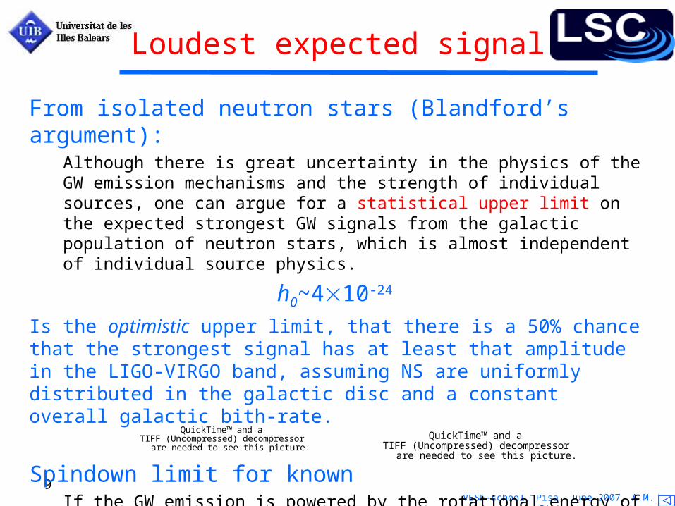
Loudest expected signal
From isolated neutron stars (Blandford’s argument):Although there is great uncertainty in the physics of the GW emission mechanisms and the strength of individual sources, one can argue for a statistical upper limit on the expected strongest GW signals from the galactic population of neutron stars, which is almost independent of individual source physics.
h0~410-24
Is the optimistic upper limit, that there is a 50% chance that the strongest signal has at least that amplitude in the LIGO-VIRGO band, assuming NS are uniformly distributed in the galactic disc and a constant overall galactic bith-rate.
Spindown limit for known pulsarsIf the GW emission is powered by the rotational energy of the NS, then one obtains: ≤ sd, h0≤ hsd
QuickTime™ and aTIFF (Uncompressed) decompressor
are needed to see this picture.
VESF-school, Pisa, June 2007, A.M. Sintes 10
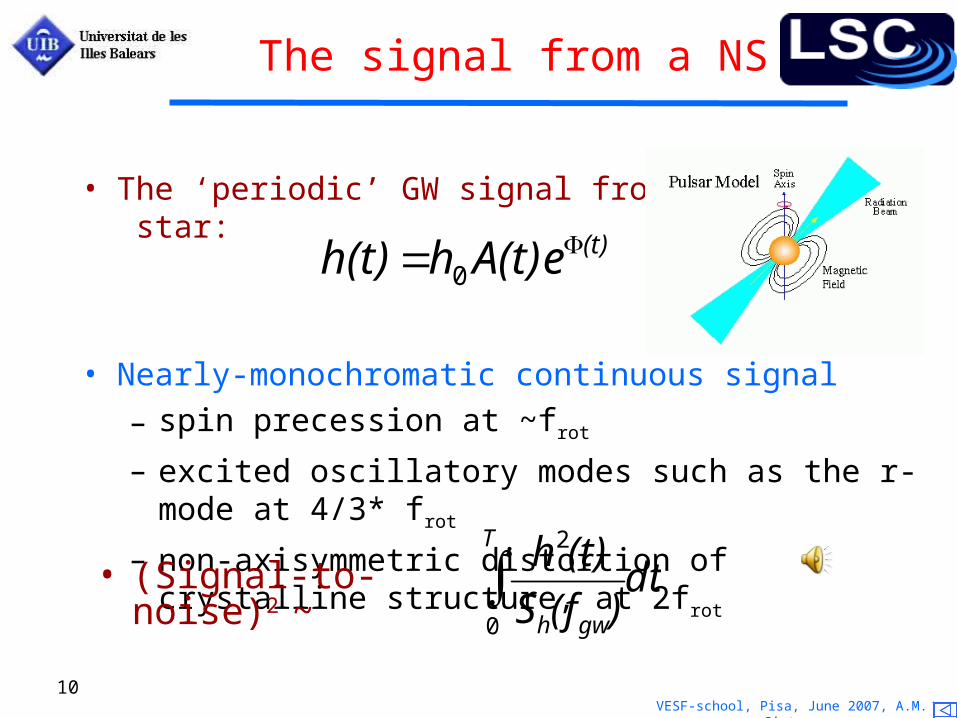
• The ‘periodic’ GW signal from a neutron star:
• Nearly-monochromatic continuous signal
– spin precession at ~frot
– excited oscillatory modes such as the r-mode at 4/3* frot
– non-axisymmetric distortion of crystalline structure, at 2frot
The signal from a NS
h(t) h0 A(t)e(t)
h2(t)
Sh(fgw)0
T
dt• (Signal-to-noise)2 ~

VESF-school, Pisa, June 2007, A.M. Sintes 11
The expected signal at the detector
A gravitational wave signal we detect from a NS will be: – Frequency modulated by relative motion of
detector and source
– Amplitude modulated by the motion of the non-uniform antenna sensitivity pattern of the detector
R
VESF-school, Pisa, June 2007, A.M. Sintes 12
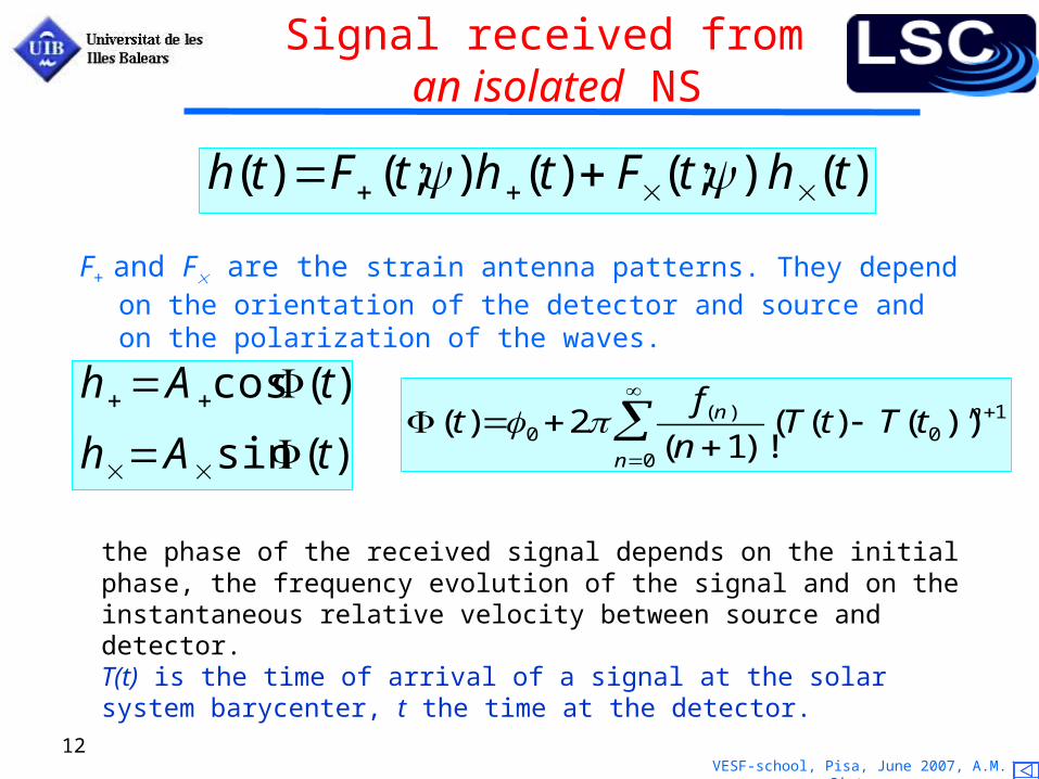
Signal received from an isolated NS
h(t) F(t;) h (t) F(t;) h(t)
F+ and F are the strain antenna patterns. They depend on the orientation of the detector and source and on the polarization of the waves.
h A cos(t)
hAsin(t)
(t)0 2f(n )
(n 1)!(T(t) T(t0))n1
n0
the phase of the received signal depends on the initial phase, the frequency evolution of the signal and on the instantaneous relative velocity between source and detector. T(t) is the time of arrival of a signal at the solar system barycenter, t the time at the detector.
VESF-school, Pisa, June 2007, A.M. Sintes 13
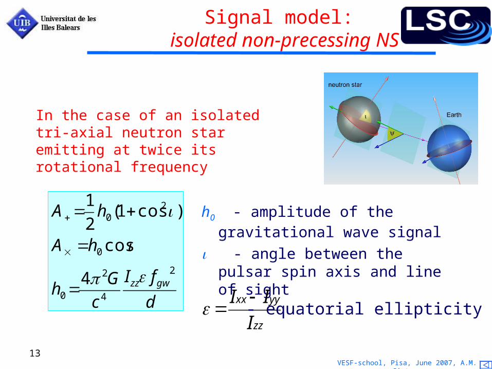
Signal model: isolated non-precessing NS
A 1
2h0(1cos2 )
A h0 cos
h0 4 2G
c 4
Izz fgw2
d
h0 - amplitude of the gravitational wave signal
- angle between the pulsar spin axis and line of sight
Ixx Iyy
Izz- equatorial ellipticity
In the case of an isolated tri-axial neutron star emitting at twice its rotational frequency
VESF-school, Pisa, June 2007, A.M. Sintes 14
Signals in noise. The meaning of probability
The strain x(t) measured by a detector is mainly dominated by noise n(t), such that even in the presence of a ignal h(t) we have
x(t)=n(t)+h(t)
Data analysis methods are not just simple recipes. We want tools capable of—dealing with very faint sources—handling very large data sets—diagnosing systematic errors—avoiding unnecessary assumptions—estimating parameters and testing models
There are different ways of proceeding depending on the paradigm of statistics used.
There are three popular interpretations of the word:Probability as a measure of our degree of belief in a statement
Probability as a measure of limiting relative frequency of outcome of a set of identical experiments
Probability as the fraction of favourable (equally likely) possibilities
We will call these the Bayesian, Frequentist and Combinatorial interpretations.
VESF-school, Pisa, June 2007, A.M. Sintes 15
Algebra of (Bayesian) probability
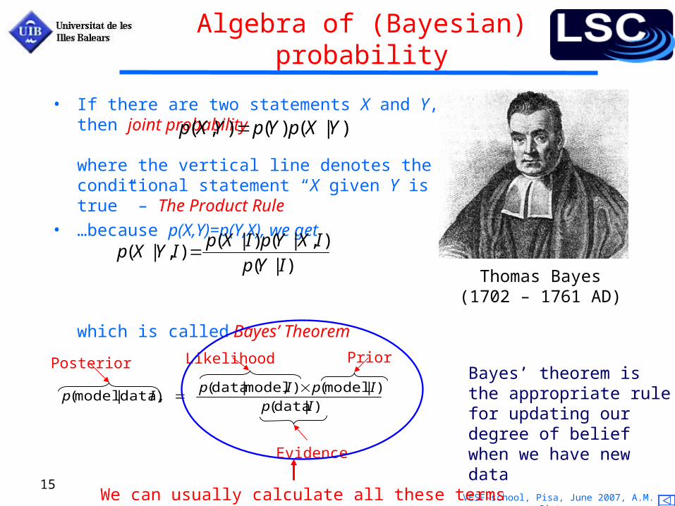
• If there are two statements X and Y, then joint probability
where the vertical line denotes the conditional statement “X given Y is true” – The Product Rule
• …because p(X,Y)=p(Y,X), we get
which is called Bayes’ Theorem
p(X |Y,I) p(X | I)p(Y | X,I)
p(Y | I)Thomas Bayes
(1702 – 1761 AD)
p(X,Y ) p(Y)p(X |Y)
p(model | data,I) p(data | model,I)p(model | I)
p(data | I)
Likelihood Prior
Evidence
Posterior
We can usually calculate all these terms
Bayes’ theorem is the appropriate rule for updating our degree of belief when we have new data
VESF-school, Pisa, June 2007, A.M. Sintes 16
Algebra of (Bayesian) probability
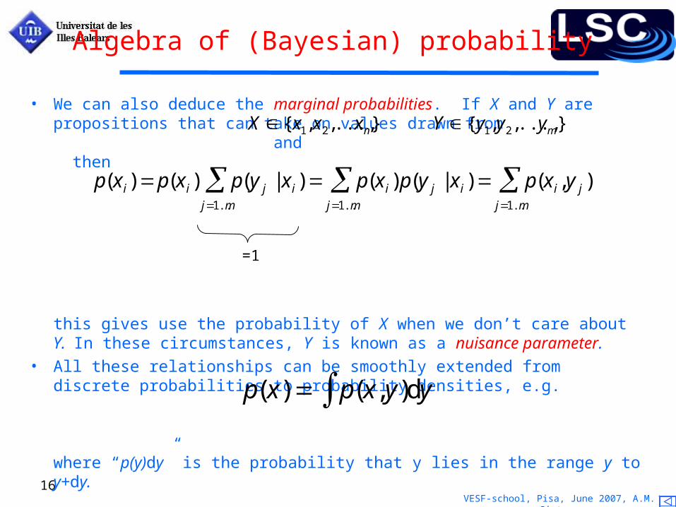
• We can also deduce the marginal probabilities. If X and Y are propositions that can take on values drawn from and then
this gives use the probability of X when we don’t care about Y. In these circumstances, Y is known as a nuisance parameter.
• All these relationships can be smoothly extended from discrete probabilities to probability densities, e.g.
where “p(y)dy” is the probability that y lies in the range y to y+dy.
X {x1, x2,..., xn},
Y {y1, y2,..., ym},
p(x i) p(x i) p(y j | x i)j1..m
p(x i)p(y j | x i)j1..m
p(x i,y j )j1..m
=1
p(x) p(x, y)dy
VESF-school, Pisa, June 2007, A.M. Sintes 17
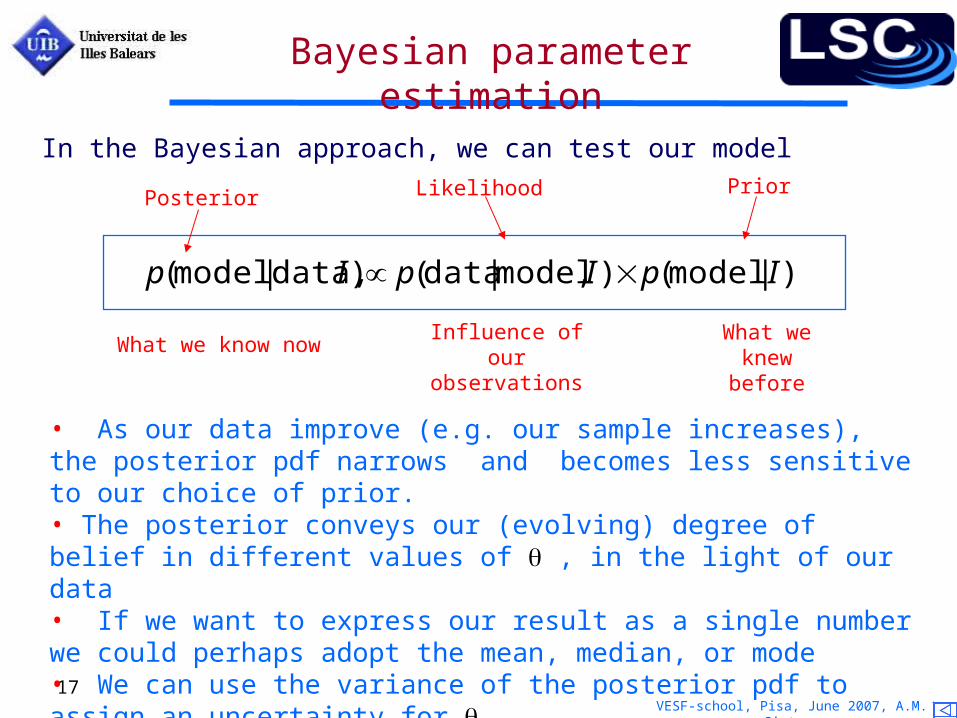
p(model | data,I) p(data | model,I)p(model | I)
Likelihood PriorPosterior
What we know nowInfluence of our
observationsWhat we
knew before
In the Bayesian approach, we can test our model
Bayesian parameter estimation
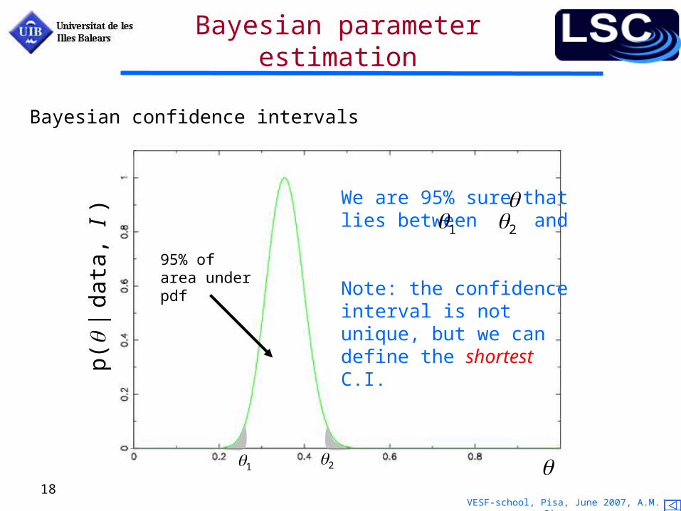
• As our data improve (e.g. our sample increases), the posterior pdf narrows and becomes less sensitive to our choice of prior.• The posterior conveys our (evolving) degree of belief in different values of , in the light of our data• If we want to express our result as a single number we could perhaps adopt the mean, median, or mode• We can use the variance of the posterior pdf to assign an uncertainty for • It is very straightforward to define confidence intervals
VESF-school, Pisa, June 2007, A.M. Sintes 18
p(
| d
ata
, I )
95% of area under pdf
12
We are 95% sure thatlies between and
Note: the confidence interval is not unique, but we can define the shortest C.I.
1 2
Bayesian confidence intervals
Bayesian parameter estimation
VESF-school, Pisa, June 2007, A.M. Sintes 19
• Recall that in frequentist (orthodox) statistics, probability is limiting relative frequency of outcome, so :
only random variables can have frequentist probabilities
as only these show variation with repeated measurement. So we can’t talk about the probability of a model parameter, or of a hypothesis. E.g., a measurement of a mass is a random variable, but the mass itself is not.
• So no orthodox probabilistic statement can be interpreted as directly referring to the parameter in question! For example, orthodox confidence intervals do not indicate the range in which we are confident the parameter value lies. That’s what Bayesian intervals do.
Frequentist framework
VESF-school, Pisa, June 2007, A.M. Sintes 20
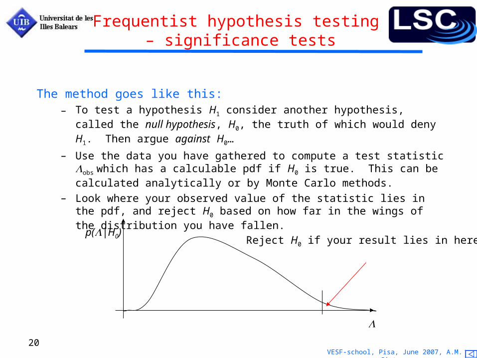
The method goes like this:– To test a hypothesis H1 consider another hypothesis, called the null hypothesis, H0, the
truth of which would deny H1. Then argue against H0…
– Use the data you have gathered to compute a test statistic obs which has a calculable pdf if H0 is true. This can be calculated analytically or by Monte Carlo methods.
– Look where your observed value of the statistic lies in the pdf, and reject H0 based on how far in the wings of the distribution you have fallen.
Frequentist hypothesis testing – significance tests
p(|H0) Reject H0 if your result lies in here
VESF-school, Pisa, June 2007, A.M. Sintes 21
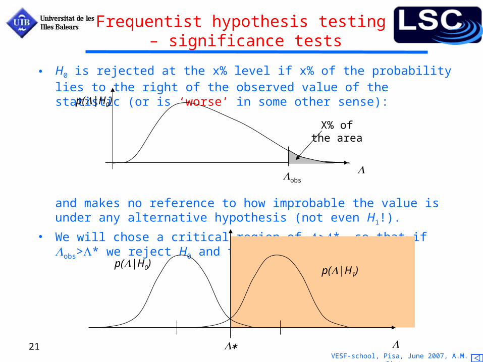
• H0 is rejected at the x% level if x% of the probability lies to the right of the observed value of the statistic (or is ‘worse’ in some other sense):
and makes no reference to how improbable the value is under any alternative hypothesis (not even H1!).
• We will chose a critical region of *, so that if obs>* we reject H0 and therefore accept H1.
Frequentist hypothesis testing – significance tests
p(|H0)
obs
X% of the area
p(|H0)
p(|H1)
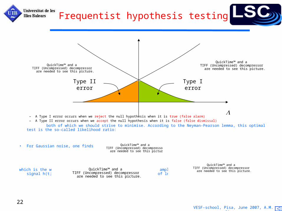
VESF-school, Pisa, June 2007, A.M. Sintes 22
– A Type I error occurs when we reject the null hypothesis when it is true (false alarm)– A Type II error occurs when we accept the null hypothesis when it is false (false dismissal)
both of which we should strive to minimise. According to the Neyman-Pearson lemma, this optimal test is the so-called likelihood ratio:
• For Gaussian noise, one finds
which is the well-known expression for the matched-filtering amplitude. If some of the parameters of the signal h(t;A,) are unknown, one has to find the maximum of lnΛ as a function of the unknown parameters
QuickTime™ and aTIFF (Uncompressed) decompressor
are needed to see this picture.
QuickTime™ and aTIFF (Uncompressed) decompressor
are needed to see this picture.
QuickTime™ and aTIFF (Uncompressed) decompressor
are needed to see this picture.
QuickTime™ and aTIFF (Uncompressed) decompressor
are needed to see this picture.
Frequentist hypothesis testing
Type II error Type I error
QuickTime™ and aTIFF (Uncompressed) decompressor
are needed to see this picture.
VESF-school, Pisa, June 2007, A.M. Sintes 23
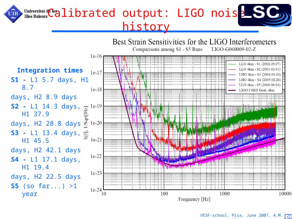
Calibrated output: LIGO noise history
Integration times
S1 - L1 5.7 days, H1 8.7
days, H2 8.9 days
S2 - L1 14.3 days, H1 37.9
days, H2 28.8 days
S3 - L1 13.4 days, H1 45.5
days, H2 42.1 days
S4 - L1 17.1 days, H1 19.4
days, H2 22.5 days
S5 (so far...) >1 year
VESF-school, Pisa, June 2007, A.M. Sintes 24
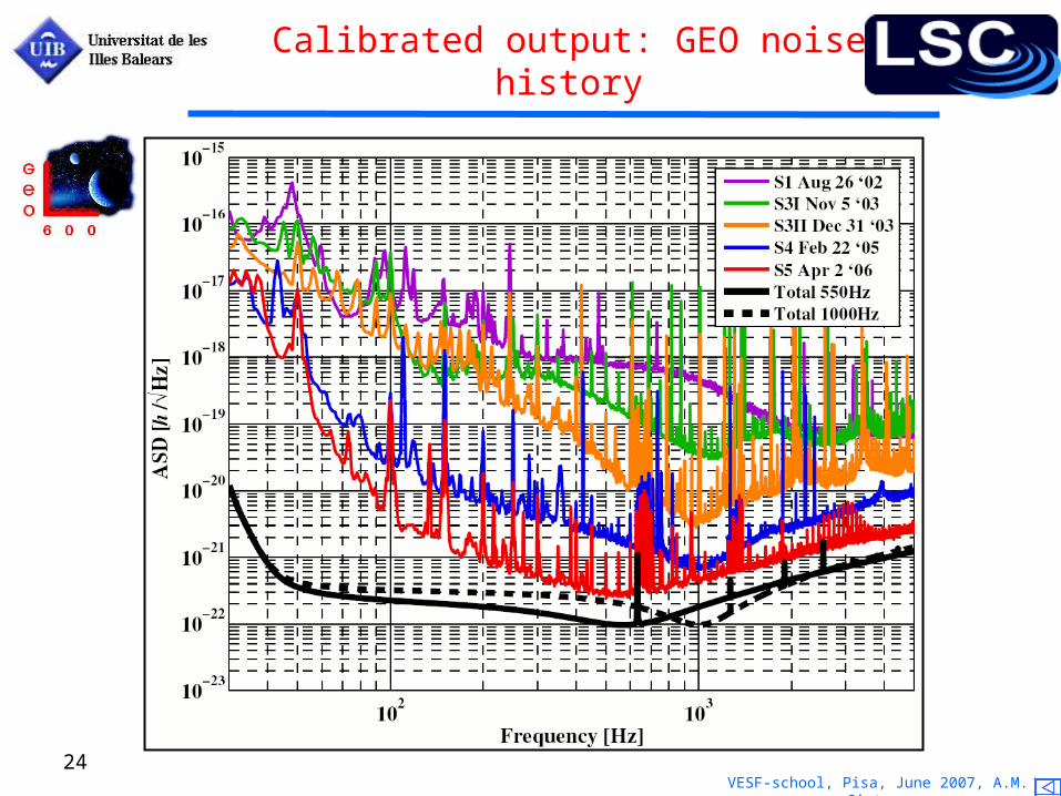
Calibrated output: GEO noise history
VESF-school, Pisa, June 2007, A.M. Sintes 25
Continuous wave searches
• Signal parameters: position (may be known), inclination angle, [orbital parameters in case of a NS in a binary system], polarization, amplitude, frequency (may be known), frequency derivative(s) (may be known), initial phase.
• Most sensitive method: coherently correlate the data with the expected signal (template) and inverse weights with the noise. If the signal were monochromatic this would be equivalent to a FT.
– Templates: we assume various sets of unknown parameters and correlate the data against these different wave-forms.
– Good news: we do not have to search explicitly over polarization, inclination, initial phase and amplitude.
• Because of the antenna pattern, we are sensitive to all the sky. Our data stream has signals from all over the sky all at once. However: low signal-to-noise is expected. Hence confusion from many sources overlapping on each other is not a concern.
• Input data to our analyses:– A calibrated data stream which with a better than 10% accuracy, is a measure of the GW excitation of the detector.
Sampling rate 16kHz (LIGO-GEO, 20kHz VIRGO), but since the high sensitivity range is 40-1500 Hz we can downsample at 3 kHz.
VESF-school, Pisa, June 2007, A.M. Sintes 26
Four neutron star populationsand searches
• Known pulsars• Position & frequency evolution known (including derivatives, timing noise, glitches, orbit)
• Unknown neutron stars• Nothing known, search over position, frequency & its derivatives
• Accreting neutron stars in low-mass x-ray binaries• Position known, sometimes orbit & frequency
• Known, isolated, non-pulsing neutron stars• Position known, search over frequency & derivatives
• What searches?– Targeted searches for signals from known pulsars
– Blind searches of previously unknown objects
– Coherent methods (require accurate prediction of the phase evolution of the signal)
– Semi-coherent methods (require prediction of the frequency evolution of the signal)
What drives the choice? The computational expense of the search
VESF-school, Pisa, June 2007, A.M. Sintes 27
Coherent detection methods
Frequency domainConceived as a module in a hierarchical search
• Matched filtering techniques. Aimed at computing a detection statistic.These methods have been implemented in the frequency domain (although this is not necessary) and are very computationally efficient.
• Best suited for large parameter space searches(when signal characteristics are uncertain)
• Frequentist approach used to cast upper limits.
Time domainprocess signal to remove frequency variations due to
Earth’s motion around Sun and spindown
• Standard Bayesian analysis, as fast numerically but provides natural parameter estimation
• Best suited to target known objects, even if phase evolution is complicated
• Efficiently handless missing data
• Upper limits interpretation: Bayesian approach
There are essentially two types of coherent searches that are performed
VESF-school, Pisa, June 2007, A.M. Sintes 28
Summary of directed pulsar searches
• Within the LIGO sensitive band (gw > 50 Hz) there are currently 163 known pulsars
• We have rotational and positional parameter information for 97 of these
• S1 (LIGO and GEO: separate analyses)– Upper limit set for GWs from J1939+2134 (h0<1.4 x 10⁻²²)– Phys. Rev. D 69, 082004 (2004)
• S2 science run (LIGO: 3 interferometers coherently, TDS)– End-to-end validation with 2 hardware injections– Upper limits set for GWs from 28 known isolated pulsars– Phys. Rev. Lett. 94, 181103 (2005)
• S3 & S4 science runs (LIGO and GEO: up to 4 interferometers coherently, TDS) – Additional hardware injections in both GEO and LIGO– Add known binary pulsars to targeted search – Full results with total of 93 (33 isolated, 60 binary) pulsars
• S5 science run (ongoing, TDS) – 32 known isolated, 41 in binaries, 29 in globular clusters
VESF-school, Pisa, June 2007, A.M. Sintes 29
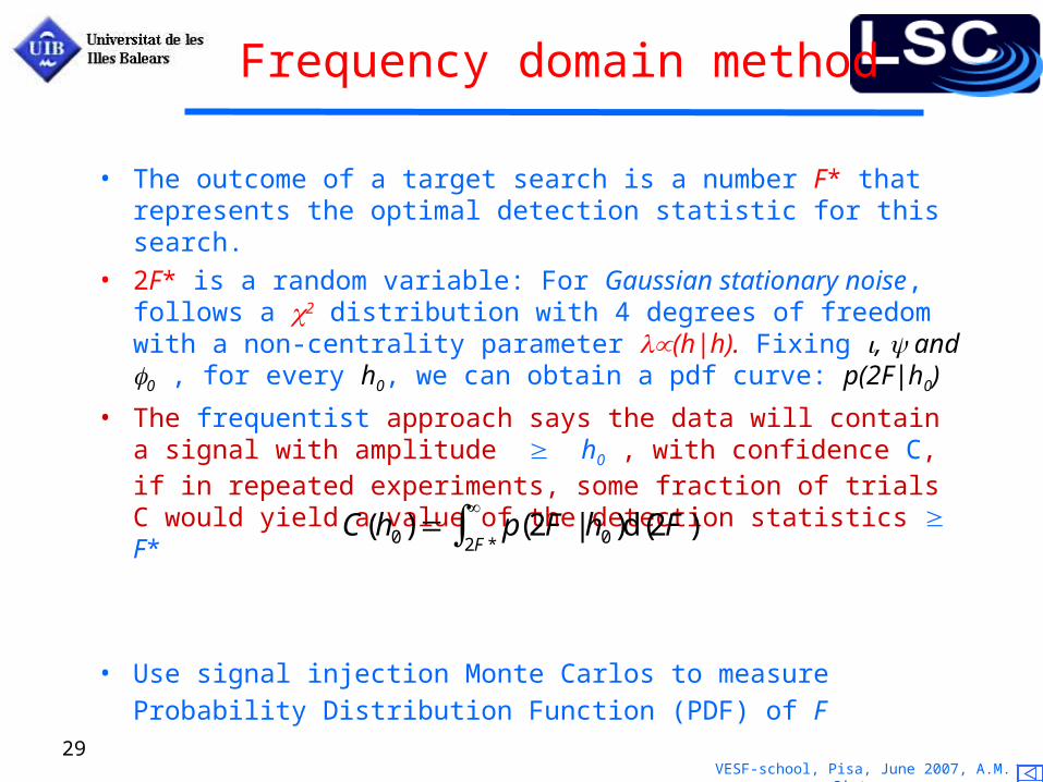
Frequency domain method
• The outcome of a target search is a number F* that represents the optimal detection statistic for this search.
• 2F* is a random variable: For Gaussian stationary noise, follows a 2 distribution with 4 degrees of freedom with a non-centrality parameter (h|h). Fixing , and 0 , for every h0, we can obtain a pdf curve: p(2F|h0)
• The frequentist approach says the data will contain a signal with amplitude h0 , with confidence C, if in repeated experiments, some fraction of trials C would yield a value of the detection statistics F*
• Use signal injection Monte Carlos to measure Probability Distribution
Function (PDF) of F
C(h0) p(2F | h0)d(2F)2F*
VESF-school, Pisa, June 2007, A.M. Sintes 30
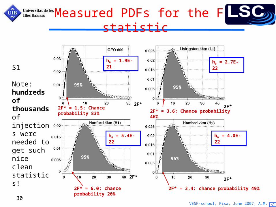
Measured PDFs for the F statistic with fake injected worst-case signals at nearby frequencies
2F* = 1.5: Chance probability 83%
2F*2F*
2F*2F*
2F* = 3.6: Chance probability 46%
2F* = 6.0: chance probability 20% 2F* = 3.4: chance probability 49%
h0 = 1.9E-21
95%95%
95%95%
h0 = 2.7E-22
h0 = 5.4E-22 h0 = 4.0E-22
S1
Note: hundreds of thousands of injections were needed to get such nice clean statistics!
VESF-school, Pisa, June 2007, A.M. Sintes 31
F-statistics
We can express h(t) in terms of amplitude A {A+, A, , 0} and Doppler parameters
QuickTime™ and aTIFF (Uncompressed) decompressor
are needed to see this picture.
QuickTime™ and aTIFF (Uncompressed) decompressor
are needed to see this picture.
QuickTime™ and aTIFF (Uncompressed) decompressor
are needed to see this picture.
QuickTime™ and aTIFF (Uncompressed) decompressor
are needed to see this picture.
QuickTime™ and aTIFF (Uncompressed) decompressor
are needed to see this picture.
VESF-school, Pisa, June 2007, A.M. Sintes 32
QuickTime™ and aTIFF (Uncompressed) decompressor
are needed to see this picture.
F-Statistics
• Analytically maximize the likelihood over A
QuickTime™ and aTIFF (Uncompressed) decompressor
are needed to see this picture.
QuickTime™ and aTIFF (Uncompressed) decompressor
are needed to see this picture.
QuickTime™ and aTIFF (Uncompressed) decompressor
are needed to see this picture.
QuickTime™ and aTIFF (Uncompressed) decompressor
are needed to see this picture.
QuickTime™ and aTIFF (Uncompressed) decompressor
are needed to see this picture.
VESF-school, Pisa, June 2007, A.M. Sintes 33
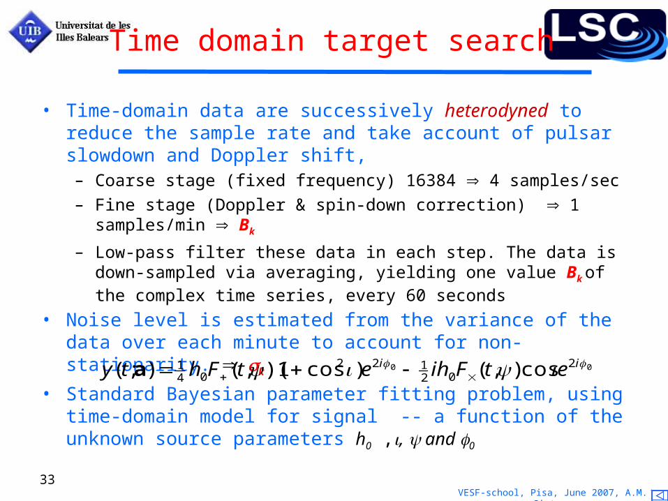
Time domain target search
• Time-domain data are successively heterodyned to reduce the sample rate and take account of pulsar slowdown and Doppler shift, – Coarse stage (fixed frequency) 16384 4 samples/sec
– Fine stage (Doppler & spin-down correction) 1 samples/min Bk
– Low-pass filter these data in each step. The data is down-sampled via averaging, yielding one value Bk of the complex time series, every 60 seconds
• Noise level is estimated from the variance of the data over each minute to account for non-stationarity. k
• Standard Bayesian parameter fitting problem, using time-domain model for signal -- a function of the unknown source parameters h0 ,, and 0
y(t;a) 14 h0F(t,)(1 cos2)e2i0 1
2 ih0F(t,)cose2i0
VESF-school, Pisa, June 2007, A.M. Sintes 34
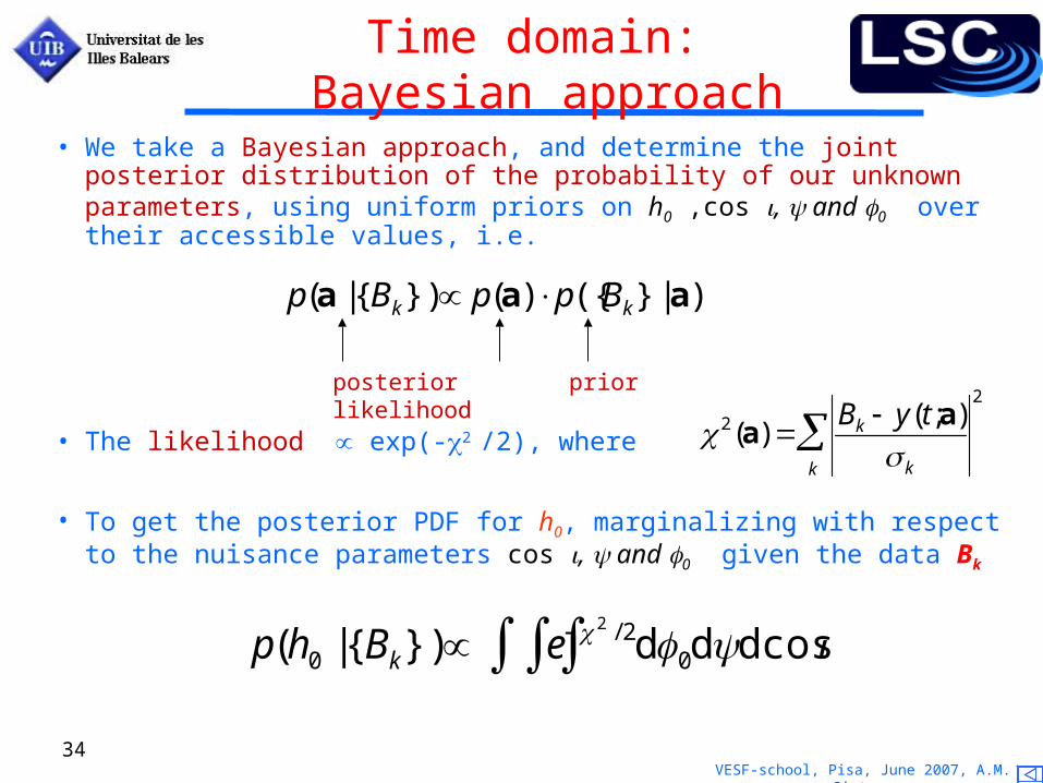
• We take a Bayesian approach, and determine the joint posterior distribution of the probability of our unknown parameters, using uniform priors on h0 ,cos , and 0 over their accessible values, i.e.
• The likelihood exp(-2 /2), where
• To get the posterior PDF for h0, marginalizing with respect to the nuisance parameters cos , and 0 given the data Bk
Time domain: Bayesian approach
p(a |{Bk}) p(a)p({Bk} | a)
posterior prior likelihood
2(a) Bk y(t;a)
k
2
k
p(h0 |{Bk}) e 2 / 2d0d dcos
VESF-school, Pisa, June 2007, A.M. Sintes 35
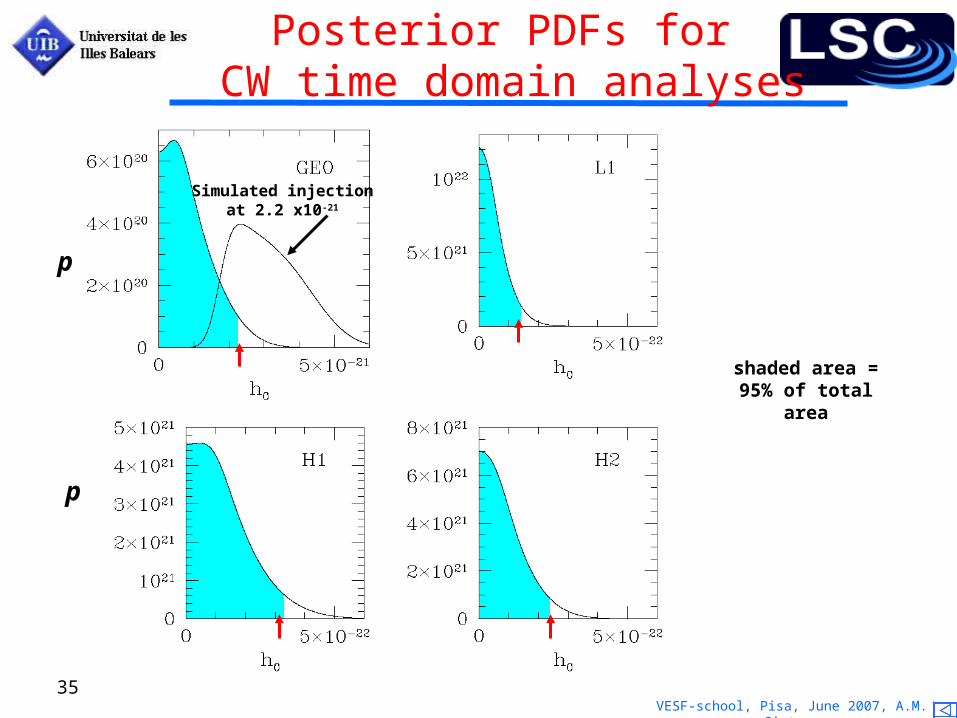
Posterior PDFs for CW time domain analyses
Simulated injectionat 2.2 x10⁻²¹
p
shaded area = 95% of total area
p
VESF-school, Pisa, June 2007, A.M. Sintes 36
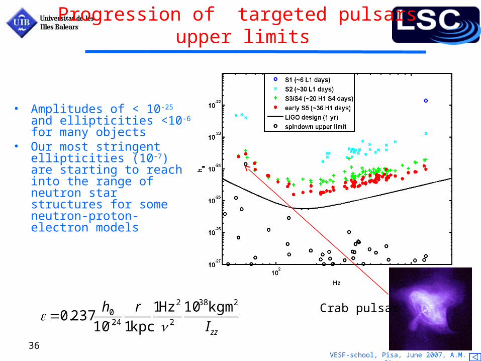
Progression of targeted pulsars upper limits
Crab pulsar
• Amplitudes of < 10-25 and ellipticities <10-6 for many objects
• Our most stringent ellipticities (10-7) are starting to reach into the range of neutron star structures for some neutron-proton-electron models
0.237h0
10 24
r
1kpc
1Hz2
2
1038kgm2
Izz
APS Meeting, Jacksonville, April 2007
VESF-school, Pisa, June 2007, A.M. Sintes 37
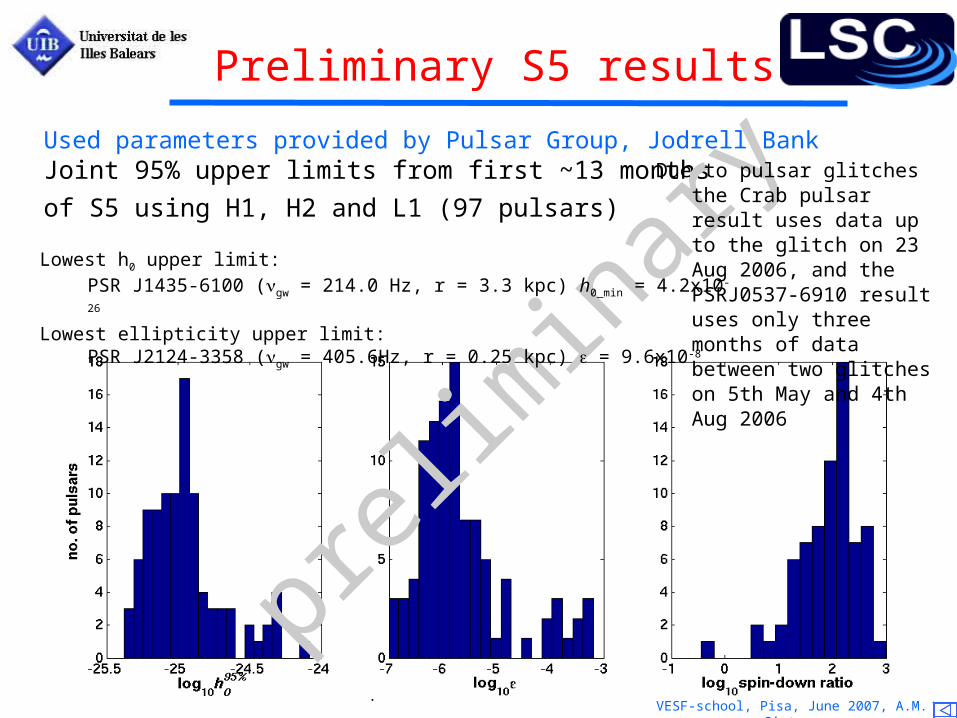
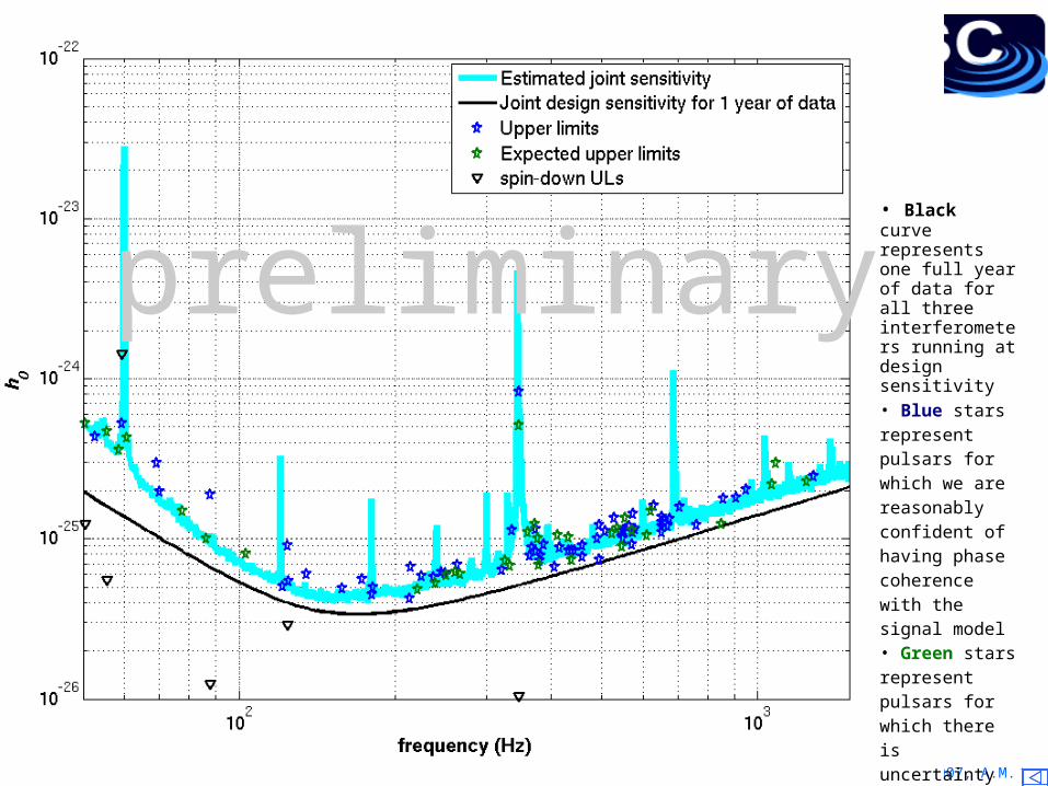
Preliminary S5 results
Used parameters provided by Pulsar Group, Jodrell Bank Joint 95% upper limits from first ~13 months
of S5 using H1, H2 and L1 (97 pulsars)
prelim
inar
yLowest h0 upper limit:
PSR J1435-6100 (gw = 214.0 Hz, r = 3.3 kpc) h0_min = 4.2x10⁻²⁶
Lowest ellipticity upper limit:PSR J2124-3358 (gw = 405.6Hz, r = 0.25 kpc) = 9.6x10⁻⁸
Due to pulsar glitches the Crab pulsar result uses data up to the glitch on 23 Aug 2006, and the PSRJ0537-6910 result uses only three months of data between two glitches on 5th May and 4th Aug 2006
APS Meeting, Jacksonville, April 2007
VESF-school, Pisa, June 2007, A.M. Sintes 38
preliminary• Black curve represents one full year of data for all three interferometers running at design sensitivity• Blue stars represent pulsars for which we are reasonably confident of having phase coherence with the signal model• Green stars represent pulsars for which there is uncertainty about phase coherence
VESF-school, Pisa, June 2007, A.M. Sintes 39
Blind searches and coherent detection methods
• Coherent methods are the most sensitive methods (amplitude SNR increases with sqrt of observation time) but they are the most computationally expensive,
why?– Our templates are constructed based on different values of the signal
parameters (e.g. position, frequency and spindown)
– The parameter resolution increases with longer observations
– Sensitivity also increases with longer observations
– As one increases the sensitivity of the search, one also increases the number of templates one needs to use.
VESF-school, Pisa, June 2007, A.M. Sintes 40
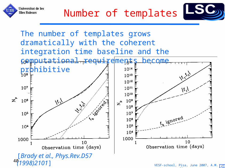
Number of templates
[Brady et al., Phys.Rev.D57 (1998)2101]
The number of templates grows dramatically with the coherent integration time baseline and the computational requirements become prohibitive

VESF-school, Pisa, June 2007, A.M. Sintes 41
S2 run: Coherent search for unknown isolated sources and Sco-X1
• Entire sky search
• Fully coherent matched filtering
• 160 to 728.8 Hz
• df/dt < 4 x 10⁻¹⁰ Hz/s
• 10 hours of S2 data; computationally intensive
• 95% confidence upper limit on the GW strain amplitude range from 6.6x10⁻²³ to 1.0x10⁻²¹ across the frequency band
• Scorpius X-1
• Fully coherent matched filtering
• 464 to 484 Hz, 604 to 624 Hz
• df/dt < 1 x 10⁻⁹ Hz/s
• 6 hours of S2 data
• 95% confidence upper limit on the GW strain amplitude range from 1.7x10⁻²² to 1.3x10⁻²¹ across the two 20 Hz wide frequency bands
• See gr-qc/0605028

VESF-school, Pisa, June 2007, A.M. Sintes 42
Computational Engine
Searchs offline at:• Medusa, Nemo clusters
(UWM)• Merlin, Morgane cluster
(AEI)• Tsunami (B’ham)• Others
VESF-school, Pisa, June 2007, A.M. Sintes 43
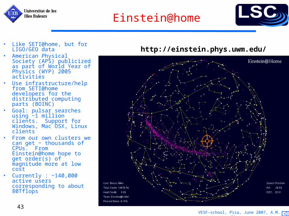
Einstein@home
http://einstein.phys.uwm.edu/• Like SETI@home, but for
LIGO/GEO data• American Physical Society
(APS) publicized as part of World Year of Physics (WYP) 2005 activities
• Use infrastructure/help from SETI@home developers for the distributed computing parts (BOINC)
• Goal: pulsar searches using ~1 million clients. Support for Windows, Mac OSX, Linux clients
• From our own clusters we can get ~ thousands of CPUs. From Einstein@home hope to get order(s) of magnitude more at low cost
• Currently : ~140,000 active users corresponding to about 80Tflops
VESF-school, Pisa, June 2007, A.M. Sintes 44
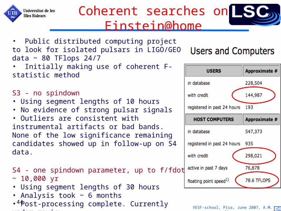
• Public distributed computing project to look for isolated pulsars in LIGO/GEO data ~ 80 TFlops 24/7• Initially making use of coherent F-statistic method
S3 - no spindown • Using segment lengths of 10 hours• No evidence of strong pulsar signals • Outliers are consistent with instrumental artifacts or bad bands. None of the low significance remaining candidates showed up in follow-up on S4 data.
S4 - one spindown parameter, up to f/fdot ~ 10,000 yr• Using segment lengths of 30 hours• Analysis took ~ 6 months• Post-processing complete. Currently under review.
S5 (R1)- similar to S4• Faster more efficient application• Currently in post-processing stage
Coherent searches onEinstein@home
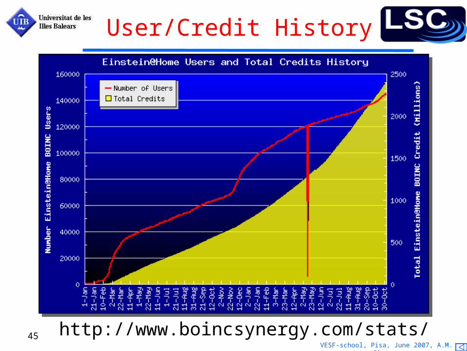
VESF-school, Pisa, June 2007, A.M. Sintes 45 http://www.boincsynergy.com/stats/
User/Credit History
VESF-school, Pisa, June 2007, A.M. Sintes 46
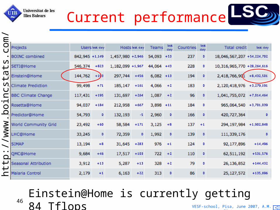
Current performance
Einstein@Home is currently getting 84 Tflops
http
://w
ww
.boi
ncst
ats.
com
/
VESF-school, Pisa, June 2007, A.M. Sintes 47
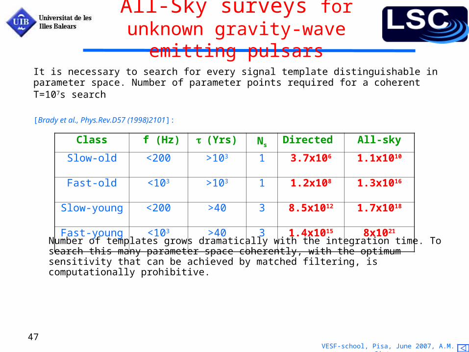
All-Sky surveys for unknown gravity-wave emitting pulsars
It is necessary to search for every signal template distinguishable in parameter space. Number of parameter points required for a coherent T=107s search
[Brady et al., Phys.Rev.D57 (1998)2101]:
Number of templates grows dramatically with the integration time. To search this many parameter space coherently, with the optimum sensitivity that can be achieved by matched filtering, is computationally prohibitive.
Class f (Hz) (Yrs) NsDirected All-sky
Slow-old <200 >103 1 3.7x10⁶ 1.1x10¹⁰
Fast-old <103 >103 1 1.2x10⁸ 1.3x10¹⁶
Slow-young <200 >40 3 8.5x10¹² 1.7x10¹⁸
Fast-young <103 >40 3 1.4x10¹⁵ 8x10²¹
VESF-school, Pisa, June 2007, A.M. Sintes 48
Coherent wide-parameter searches
• The second effect of the large number of templates Np is to reduce the sensitivity compared to a targeted search with the same observation time and false-alarm probability: increasing the number of templates increases the number of expected false-alarm candidates at fixed detection threshold. Therefore the detection-threshold needs to be raised to maintain the same false-alarm rate, thereby decreasing the sensitivity.
• Note that increasing the number of equal-sensitivity detectors N improves the SNR in the same way as increasing the integration time Tobs. However, increasing the number of detectors N does — contrary to the observation time Tobs — not increase the required number of templates Np, which makes this the computationally cheapest way to improve the SNR of coherent wide-parameter searches.
VESF-school, Pisa, June 2007, A.M. Sintes 49
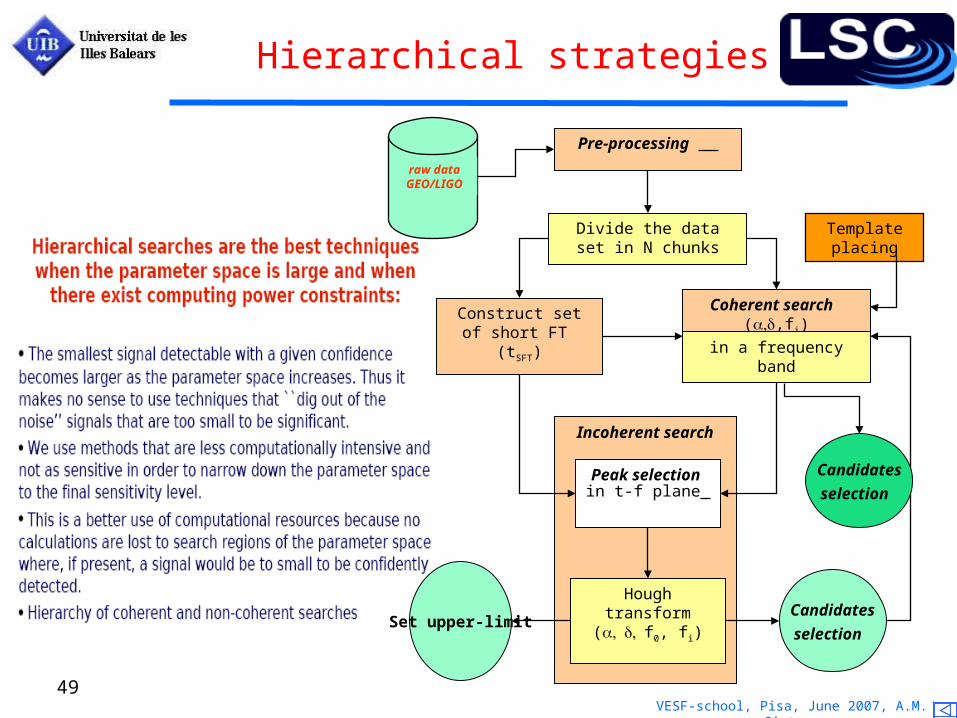
Hierarchical strategies
Set upper-limit
Pre-processing
Divide the data set in N chunks
raw data GEO/LIGO
Construct set of short FT (tSFT)
Coherent search (,fi)
in a frequency band
Template placing
Incoherent search
Hough transform(f0, fi)
Peak selection in t-f plane
Candidates
selection
Candidates
selection
VESF-school, Pisa, June 2007, A.M. Sintes 50
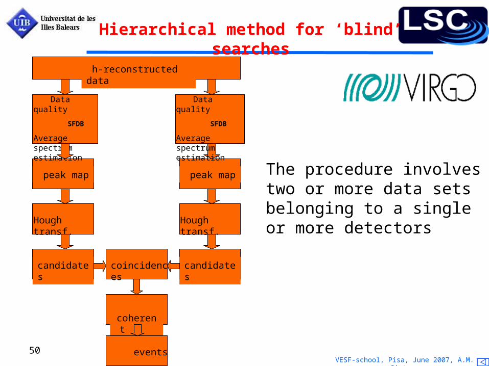
Hierarchical method for ‘blind’ searches
h-reconstructed data
Data quality
SFDB
Average spectrum estimation
peak map
Hough transf.
candidates
peak map
Hough transf.
candidatescoincidences
coherent step
events
Data quality
SFDB
Average spectrum estimation
The procedure involves two or more data sets belonging to a single or more detectors
VESF-school, Pisa, June 2007, A.M. Sintes 51
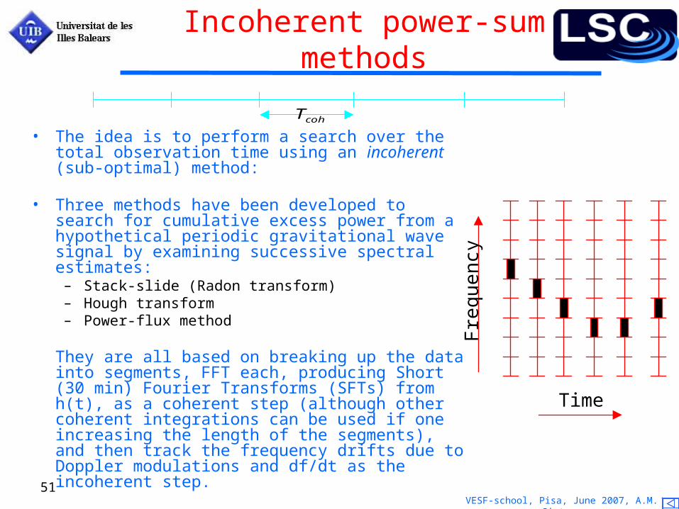
Incoherent power-sum methods
• The idea is to perform a search over the total observation time using an incoherent (sub-optimal) method:
• Three methods have been developed to search for cumulative excess power from a hypothetical periodic gravitational wave signal by examining successive spectral estimates:
– Stack-slide (Radon transform)– Hough transform– Power-flux method
They are all based on breaking up the data into segments, FFT each, producing Short (30 min) Fourier Transforms (SFTs) from h(t), as a coherent step (although other coherent integrations can be used if one increasing the length of the segments), and then track the frequency drifts due to Doppler modulations and df/dt as the incoherent step.
cohT
Fre
quen
cy
Time

VESF-school, Pisa, June 2007, A.M. Sintes 52
Differences among the incoherent methods
What is exactly summed?
• StackSlide – Normalized power (power divided by estimated noise) Averaging gives expectation of 1.0 in absence of signal
• Hough – Weighted binary counts (0/1 = normalized power below/above SNR), with weighting based on antenna pattern and detector noise
• PowerFlux – Average strain power with weighting based on antenna pattern and detector noise Signal estimator is direct excess strain noise(circular polarization and 4 linear polarization projections)

VESF-school, Pisa, June 2007, A.M. Sintes 53
Peak selection in the t-f plane
• Input data: Short Fourier Transforms (SFT) of time series
• For every SFT, select frequency bins i such exceeds some threshold th
time-frequency plane of zeros and ones
• p(|h, Sn) follows a 2 distribution with 2 degrees of freedom:
• The false alarm and detection probabilities for a threshold thare
i | ˜ x (f i) |2
| ˜ n (f i) |2
i 4 | ˜ h (f i) |2
Sn(f i)TSFT
i 1i
2
2 1 i
(th | Sn ) p( th
| 0,Sn )d e th ,
(th | h,Sn ) p( th
| h,Sn )d
˜ x (f) ˜ n (f) ˜ h (f)
VESF-school, Pisa, June 2007, A.M. Sintes 54
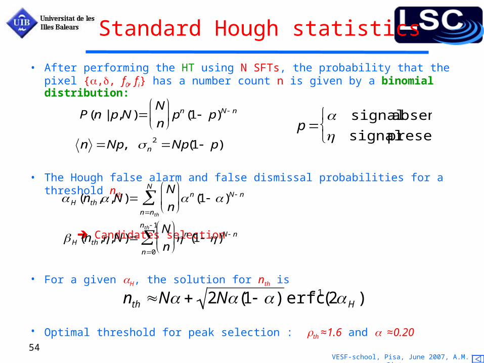
Standard Hough statistics
• After performing the HT using N SFTs, the probability that the pixel {,, f0, fi} has a number count n is given by a binomial distribution:
• The Hough false alarm and false dismissal probabilities for a threshold nth
Candidates selection
• For a given H, the solution for nth is
• Optimal threshold for peak selection : th ≈1.6 and ≈0.20
P(n | p,N)N
n
pn (1 p)N n
n Np, n2 Np(1 p)
p signal absent
signal present
H (nth,,N)N
n
n (1 )N n
nn th
N
H (nth,,N)N
n
n (1 )N n
n0
n th 1
nth N 2N(1 ) erfc 1(2H )
VESF-school, Pisa, June 2007, A.M. Sintes 55
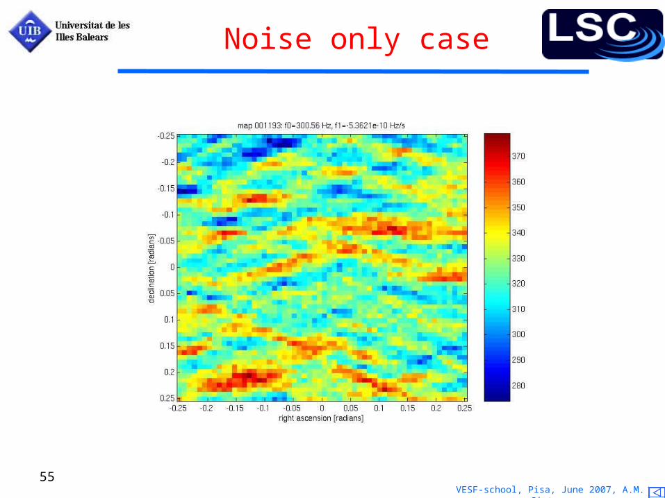
Noise only case
VESF-school, Pisa, June 2007, A.M. Sintes 56
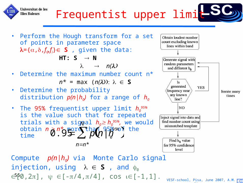
Frequentist upper limit
• Perform the Hough transform for a set of points in parameter space ={,,f0,fi} S , given the data:
HT: S N n(
• Determine the maximum number count n*n* = max (n( S
• Determine the probability distribution p(n|h0) for a range of h0
• The 95% frequentist upper limit h095% is the value such
that for repeated trials with a signal h0 h095%, we
would obtain n n* more than 95% of the time
0.95 p n|h0
95% nn*
N
Compute p(n|h0) via Monte Carlo signal injection, using S , and 0 [0,2], [-/4,/4], cos [-1,1].
VESF-school, Pisa, June 2007, A.M. Sintes 57
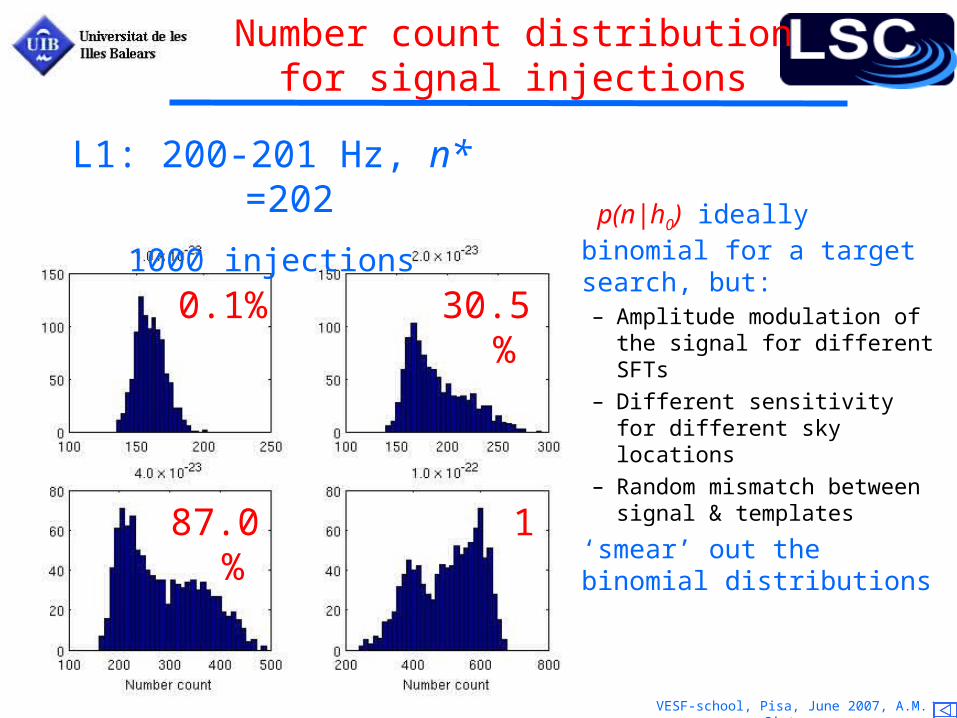
0.1% 30.5%
87.0% 1
Number count distributionfor signal injections
p(n|h0) ideally binomial for a target search, but:– Amplitude modulation of
the signal for different SFTs
– Different sensitivity for different sky locations
– Random mismatch between signal & templates
‘smear’ out the binomial distributions
L1: 200-201 Hz, n* =202
1000 injections
VESF-school, Pisa, June 2007, A.M. Sintes 58
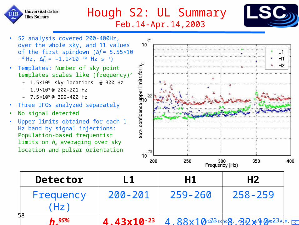
Hough S2: UL Summary Feb.14-Apr.14,2003
Detector L1 H1 H2
Frequency (Hz) 200-201 259-260 258-259
h095% 4.43x10⁻²³ 4.88x10⁻²³ 8.32x10⁻²³
• S2 analysis covered 200-400Hz, over the whole sky, and 11 values of the first spindown (Δf = 5.55×10 – 4 Hz, Δf1 = –1.1×10– 10 Hz s– 1)
• Templates: Number of sky point templates scales like (frequency)2
– 1.5×10⁵ sky locations @ 300 Hz
– 1.9×10⁹ @ 200-201 Hz
– 7.5×10⁹ @ 399-400 Hz
• Three IFOs analyzed separately
• No signal detected
• Upper limits obtained for each 1 Hz band by signal injections: Population-based frequentist limits on h0 averaging over sky location and pulsar orientation
VESF-school, Pisa, June 2007, A.M. Sintes 59
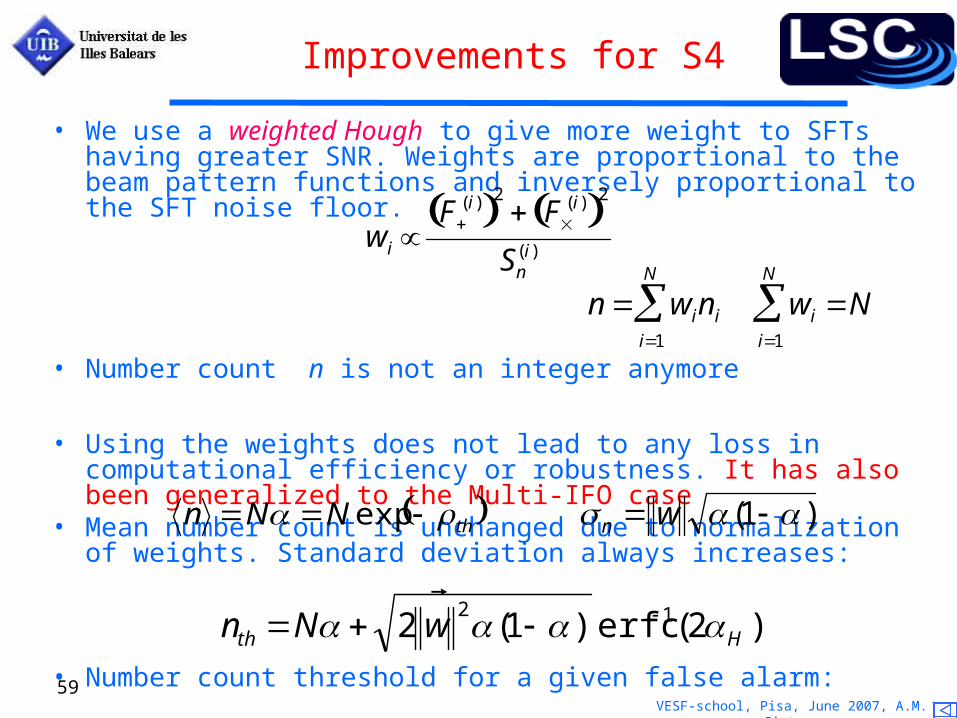
Improvements for S4
• We use a weighted Hough to give more weight to SFTs having greater SNR. Weights are proportional to the beam pattern functions and inversely proportional to the SFT noise floor.
• Number count n is not an integer anymore
• Using the weights does not lead to any loss in computational efficiency or robustness. It has also been generalized to the Multi-IFO case
• Mean number count is unchanged due to normalization of weights. Standard deviation always increases:
• Number count threshold for a given false alarm:
n wini
i1
N
wi Ni1
N
wi F
( i) 2 F( i) 2
Sn( i)
thNNn exp )1( wn
)2(erfc)1(2 12
Hth wNn

VESF-school, Pisa, June 2007, A.M. Sintes 60
Contribution of different IFOs
Figure plots the relative noise weights from H1, H2 and L1
All i
IFO i
w
w
VESF-school, Pisa, June 2007, A.M. Sintes 61
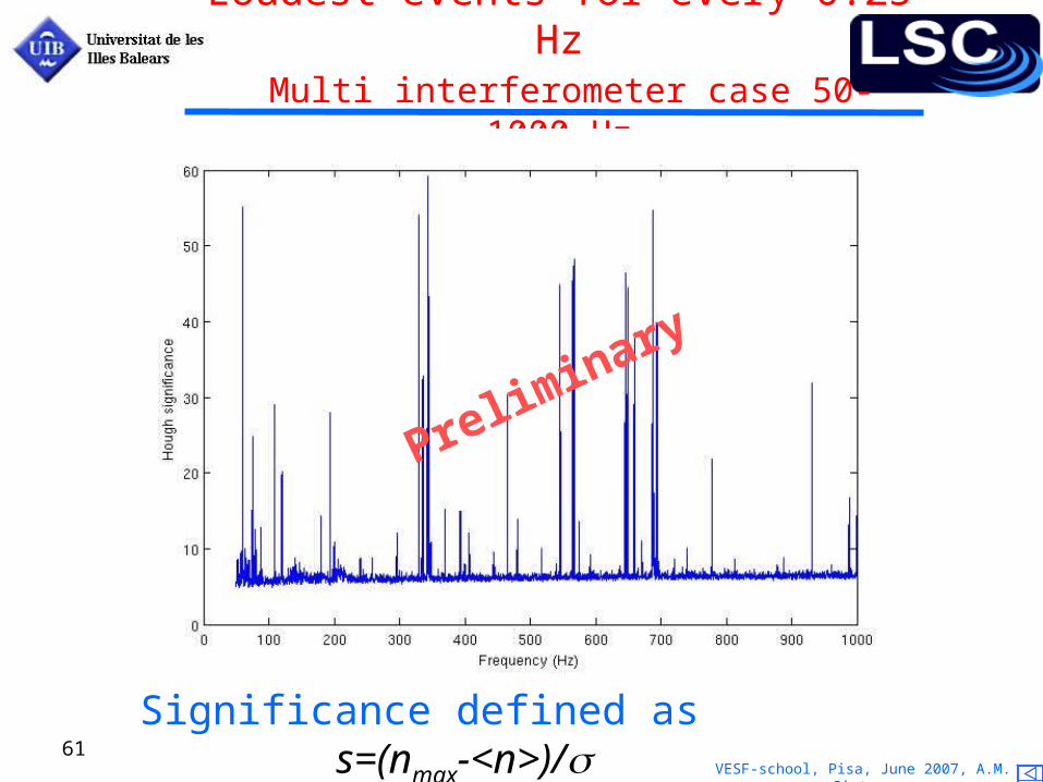
Loudest events for every 0.25 Hz Multi interferometer case 50-1000 Hz
Significance defined as s=(nmax-<n>)/
Prelim
inary

VESF-school, Pisa, June 2007, A.M. Sintes 62
The S4 Hough search
• As before, input data is a set of N 1800s SFTs (no demodulations)
• Weights allow us to use SFTs from all three IFOs together:1004 SFTS from H1, 1063 from H2 and 899 from L1
• Search frequency band 50-1000Hz• 1 spin-down parameter. Spindown
range [-2.2,0]×10-9 Hz/s with a resolution of 2.2×10⁻¹⁰ Hz/s
• All sky search• All-sky upper limits set in 0.25 Hz
bands• Multi-IFO and single IFOs have
been analyzed Best ULfor L1: 5.9×10⁻²⁴
for H1: 5.0×10⁻²⁴
for Multi H1-H2-L1: 4.3×10⁻²⁴
Prelim
inary
VESF-school, Pisa, June 2007, A.M. Sintes 63
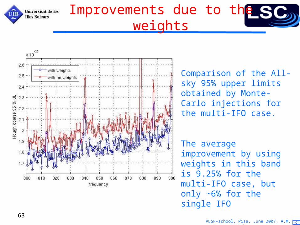
Improvements due to the weights
Comparison of the All-sky 95% upper limits obtained by Monte-Carlo injections for the multi-IFO case.
The average improvement by using weights in this band is 9.25% for the multi-IFO case, but only ~6% for the single IFO
VESF-school, Pisa, June 2007, A.M. Sintes 64
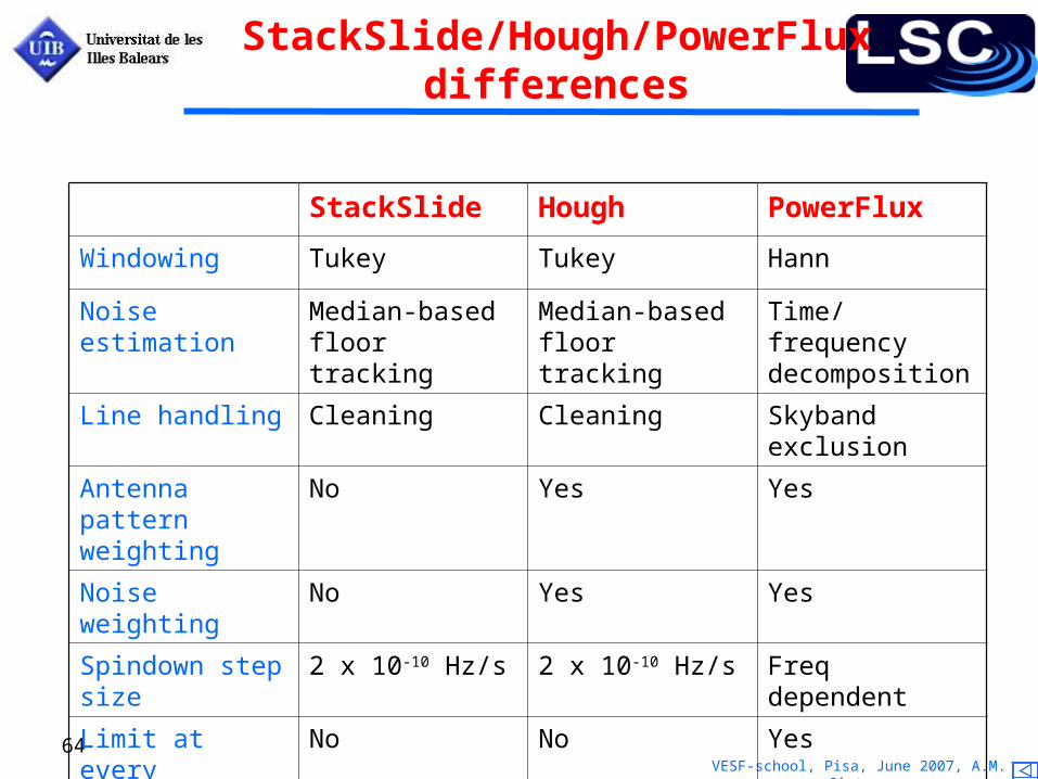
StackSlide/Hough/PowerFlux differences
StackSlide Hough PowerFlux
Windowing Tukey Tukey Hann
Noise estimation Median-based floor tracking
Median-based floor tracking
Time/frequency decomposition
Line handling Cleaning Cleaning Skyband exclusion
Antenna pattern weighting
No Yes Yes
Noise weighting No Yes Yes
Spindown step size 2 x 10⁻¹⁰ Hz/s 2 x 10⁻¹⁰ Hz/s Freq dependent
Limit at every skypoint
No No Yes
Upper limit type Population-based Population-based Strict frequentist
VESF-school, Pisa, June 2007, A.M. Sintes 65
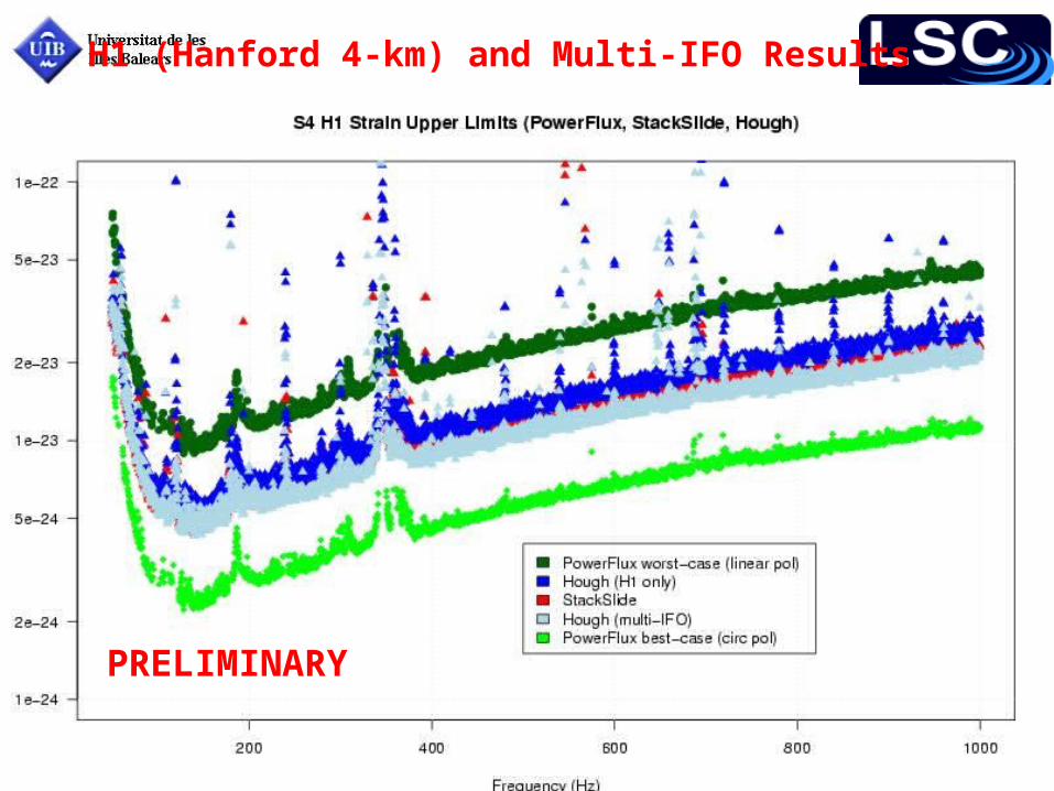
H1 (Hanford 4-km) and Multi-IFO Results
PRELIMINARY
VESF-school, Pisa, June 2007, A.M. Sintes 66
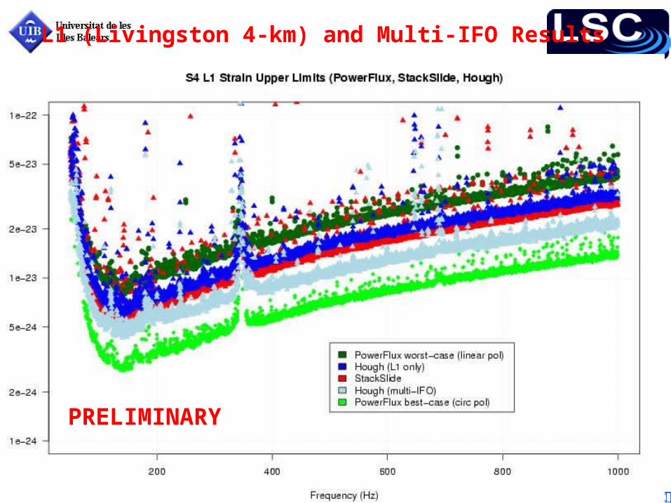
L1 (Livingston 4-km) and Multi-IFO Results
PRELIMINARY
VESF-school, Pisa, June 2007, A.M. Sintes 67
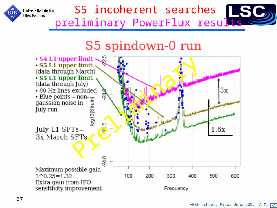
S5 incoherent searches preliminary PowerFlux results
Preliminary
VESF-school, Pisa, June 2007, A.M. Sintes 68
QuickTime™ and aTIFF (Uncompressed) decompressor
are needed to see this picture.
E@H-Hierarchical search
Basic algorithm
• Started test-run (~3 months)– currently working on improving stability & reliability
• Will be followed by a full 1-year run• Should permit a search that extends hundreds of pc into the Galaxy• This should become the most sensitive blind CW search possible with current
knowledge and technology
VESF-school, Pisa, June 2007, A.M. Sintes 69
Sensitivity estimate of different E@H Runs
QuickTime™ and aTIFF (Uncompressed) decompressor
are needed to see this picture.
VESF-school, Pisa, June 2007, A.M. Sintes 70
Searches for Continuous Waves, present, past and future
QuickTime™ and aTIFF (Uncompressed) decompressor
are needed to see this picture.
VESF-school, Pisa, June 2007, A.M. Sintes 71
Conclusions
• Analysis of LIGO data is in full swing, and results from LIGO searches from science runs 4, 5 are now appearing.– Significant improvements in interferometer sensitivity since S3.– In the process of accumulating 1 year of data (S5).– Known pulsar searches are beginning to place interesting upper
limits in S5
– All sky searches are under way and exploring large area of parameter space
• Veto strategies and data conditioning are becoming more relevant in order to reduce the selection threshold and improve sensitivity