algorithmic self-assembly of dna - center for bits and atoms
TRANSCRIPT

Algorithmic Self-Assembly of DNA
Thesis byErik Winfree
In Partial Fulfillment of the Requirementsfor the Degree of
Doctor of Philosophy
1 8 9 1
CA
LIF
OR
NIA
I
NS T IT U T E O F T
EC
HN
OL
OG
Y
California Institute of TechnologyPasadena, California
1998(Submitted May 19, 1998)

ii
c 1998Erik Winfree
All Rights Reserved

iii
Acknowledgements
This thesis reports an unusual and unexpected journey through intellectual territory entirely newto me. Who is prepared for such journeys? I was not. Thus my debt is great to those who havehelped me along the way, without whose help I would have been completely lost and uninspired.
There is no way to give sufficient thanks to my advisor, John Hopfield. His encouragementfor me to get my feet wet, and his advice cutting to the bone of each issue, have been invaluable.John’s policy has been, in his own words, to give his students “enough rope to hang themselveswith.” But he knows full well that a lot of rope is needed to weave macrame. Perhaps the onlypossible repayment is in kind: to maintain a high standard of integrity, and when my turn comes,to provide a nurturing environment for other young minds.
Len Adleman and Ned Seeman have each been mentors during my thesis work. In many ways,my research can be seen as the direct offspring of their work, combining the notion of using DNAfor computation with the ability to design DNA structures with artificial topology. Both Len andNed have provided encouragement, support, and valuable feedback throughout this project.
I would like additionally to thank Ned Seeman and Xiaoping Yang for teaching me how todo laboratory experiments with DNA. Xiaoping’s patient and careful tutoring provided me witha solid first step toward becoming a competent experimenter. John Abelson generously made mewelcome to continue my experimenting at Caltech in a friendly and expert environment; I amdeeply grateful to him and to all the members of his laboratory without whose help I could havedone little. For teaching me to use the atomic force microscope, I thank Anca Segall, Bob Moision,and Ely Rabani; with their encouragement and help I saw the first exciting images of DNA lattices.Likewise, Rob Rossi’s friendly and spirited management of the Caltech SPM room made doingscience there a breeze.
I am grateful for the encouragement and feedback of my thesis committee: John Abelson,Yaser Abu-Mostafa, Len Adleman, John Baldeschwieler, Al Barr, and John Hopfield.
Perhaps most influential have been the people in my everyday life. All the members of theHopfield group – Carlos Brody, Dawei Dong, Maneesh Sahani, Marcus Mitchell, Sam Roweis,Sanjoy Majahan, Tom Annau, and Unni Unnikrishnan – have been wonderful to be with, both onand off duty. Laura Rodriguez has been our guardian angel. Paul Rothemund has been a steadyand stimulating companion throughout this DNA adventure, and it is fair to say that this projectwould never have been born without him. Matt Cook has been a source of intellectual inspirationand joy for many years. I have learned so much from you all. I will miss you all when we areapart; let those times be brief!
I must add that I feel very fortunate to have come to a place – Caltech’s CNS program –where as a naive mathematician and computer scientist, I can build an autonomous robot car,do electrophysiology on the brain of rat and listen to the cries of the jungle therein, and weavemacrame out of life’s genetic molecules. There’s nothing else like it. Therefore I also wantto thank Caltech and all the people that compose it’s unique community. Nowhere have I feltintellectually more at home, and among people like myself.
I am grateful for stimulating discussions with many scientists in the wider community, in-cluding John Reif, Dan Abrahams-Gessel, Tony Eng, Natasha Jonoska, James Wetmur, and manyothers. I thank Takashi Yokomori for inviting me and hosting me on a once-in-a-lifetime trip toJapan, where I was able to share ideas with a great number of people who think about DNA com-puting; I would like to name in particular Masami Hagiya, Shigeyuki Yokoyama, Masanori Arita,

iv
Akira Suyama, Satoshi Kobayashi, and Kozuyoshi Harada.Reaching further into the past, I would like to thank Stephen Wolfram for the experience of
working with him in 1991-1992, and for introducing me to many exciting areas of thought incellular automata, complex systems, and the nature of computation.
A special thanks to Hui Wang, for her wisdom and for her love.Finally, all thanks must come to the source of who I am: my parents and my family. Thanks
Mom, thanks Dad, for all the ways you have nurtured my growth, stimulated me and left me tomy own devices, encouraged me and provided for me, given me good counsel and strong love.

v
Abstract
How can molecules compute? In his early studies of reversible computation, Bennett imagined anenzymatic Turing Machine which modified a hetero-polymer (such as DNA) to perform computa-tion with asymptotically low energy expenditures. Adleman’s recent experimental demonstrationof a DNA computation, using an entirely different approach, has led to a wealth of ideas for howto build DNA-based computers in the laboratory, whose energy efficiency, information density,and parallelism may have potential to surpass conventional electronic computers for some pur-poses. In this thesis, I examine one mechanism used in all designs for DNA-based computer –the self-assembly of DNA by hybridization and formation of the double helix – and show that thismechanism alone in theory can perform universal computation. To do so, I borrow an importantresult in the mathematical theory of tiling: Wang showed how jigsaw-shaped tiles can be designedto simulate the operation of any Turing Machine. I propose constructing molecular Wang tilesusing the branched DNA constructions of Seeman, thereby producing self-assembled and algo-rithmically patterned two-dimensional lattices of DNA. Simulations of plausible self-assemblykinetics suggest that low error rates can be obtained near the melting temperature of the lattice;under these conditions, self-assembly is performing reversible computation with asymptoticallylow energy expenditures. Thus encouraged, I have begun an experimental investigation of al-gorithmic self-assembly. A competition experiment suggests that an individual logical step canproceed correctly by self-assembly, while a companion experiment demonstrates that unpatternedtwo dimensional lattices of DNA will self-assemble and can be visualized. We have reason tohope, therefore, that this experimental system will prove fruitful for investigating issues in thephysics of computation by self-assembly. It may also lead to interesting new materials.

vi
Contents
Acknowledgements iii
Abstract v
1 Contributions 11.1 Introduction to DNA-Based Computation . . . . . . . . . . . . . . . . . . . . . 11.2 Models of Computation by Self-Assembly . . . . . . . . . . . . . . . . . . . . . 11.3 Experiments with Self-Assembly . . . . . . . . . . . . . . . . . . . . . . . . . . 21.4 Publication List . . . . . . . . . . . . . . . . . . . . . . . . . . . . . . . . . . . 21.5 Support . . . . . . . . . . . . . . . . . . . . . . . . . . . . . . . . . . . . . . . 3
2 Introduction to DNA-Based Computation 52.1 Why Compute with Molecules, and How? . . . . . . . . . . . . . . . . . . . . . 52.2 Computing Inverse Sets with DNA . . . . . . . . . . . . . . . . . . . . . . . . . 5
2.2.1 Abstract Models of Molecular Computation . . . . . . . . . . . . . . . . 72.2.2 Branching Programs . . . . . . . . . . . . . . . . . . . . . . . . . . . . 102.2.3 Correspondence of Models . . . . . . . . . . . . . . . . . . . . . . . . . 112.2.4 Corollaries and Conclusions . . . . . . . . . . . . . . . . . . . . . . . . 132.2.5 Discussion . . . . . . . . . . . . . . . . . . . . . . . . . . . . . . . . . 14
2.3 0(1) Methods for DNA Computation . . . . . . . . . . . . . . . . . . . . . . . . 152.3.1 Solving FSAT in O(1) biosteps . . . . . . . . . . . . . . . . . . . . . . 182.3.2 Combinatorial Sets of GOTO Programs . . . . . . . . . . . . . . . . . . 202.3.3 Single-Strand Computation of Boolean Circuits . . . . . . . . . . . . . . 232.3.4 Conclusions and Future Directions . . . . . . . . . . . . . . . . . . . . . 25
3 Models of Computation by Self-Assembly 273.1 2D Self-Assembly for Computation . . . . . . . . . . . . . . . . . . . . . . . . 27
3.1.1 Some Basic Annealing Reactions . . . . . . . . . . . . . . . . . . . . . 283.1.2 Operations Using Linear DNA . . . . . . . . . . . . . . . . . . . . . . . 303.1.3 Operations Using Branched DNA . . . . . . . . . . . . . . . . . . . . . 303.1.4 Comparison with Other Approaches . . . . . . . . . . . . . . . . . . . . 39
3.2 Graph-Theoretic Models of DNA Self-Assembly . . . . . . . . . . . . . . . . . 393.2.1 Language Theory and Grammars . . . . . . . . . . . . . . . . . . . . . . 413.2.2 DNA Complexes and Self-Assembly Rules . . . . . . . . . . . . . . . . 433.2.3 Linear Self-Assembly is Equivalent to Regular Languages . . . . . . . . 453.2.4 Dendrimer Self-Assembly is Equivalent to Context-Free Languages . . . 463.2.5 Two Dimensional Self-assembly is Universal . . . . . . . . . . . . . . . 493.2.6 Solving the Hamiltonian Path Problem . . . . . . . . . . . . . . . . . . . 503.2.7 Three Dimensional Self-Assembly Augments Computational Power . . . 523.2.8 Discussion . . . . . . . . . . . . . . . . . . . . . . . . . . . . . . . . . 54
3.3 Simulation of Self-Assembly Thermodynamics and Kinetics . . . . . . . . . . . 553.3.1 An Abstract Model of 2D Self-Assembly . . . . . . . . . . . . . . . . . 563.3.2 Implementation by Self-Assembly of DNA . . . . . . . . . . . . . . . . 60

vii
3.3.3 A Kinetic Model of DNA Self-Assembly . . . . . . . . . . . . . . . . . 623.3.4 Simulation Results . . . . . . . . . . . . . . . . . . . . . . . . . . . . . 653.3.5 Analysis . . . . . . . . . . . . . . . . . . . . . . . . . . . . . . . . . . 693.3.6 Discussion . . . . . . . . . . . . . . . . . . . . . . . . . . . . . . . . . 733.3.7 Conclusions . . . . . . . . . . . . . . . . . . . . . . . . . . . . . . . . . 76
4 Experiments with DNA Self-Assembly 784.1 A Competition Experiment: Slot-Filling . . . . . . . . . . . . . . . . . . . . . . 78
4.1.1 Materials and Methods . . . . . . . . . . . . . . . . . . . . . . . . . . . 794.1.2 Results . . . . . . . . . . . . . . . . . . . . . . . . . . . . . . . . . . . 804.1.3 Discussion . . . . . . . . . . . . . . . . . . . . . . . . . . . . . . . . . 84
4.2 Experiments with 2D Lattices . . . . . . . . . . . . . . . . . . . . . . . . . . . 854.2.1 Design of DNA Crystal . . . . . . . . . . . . . . . . . . . . . . . . . . . 864.2.2 Materials and Methods . . . . . . . . . . . . . . . . . . . . . . . . . . . 884.2.3 Results of Characterization by Gel Electrophoresis . . . . . . . . . . . . 894.2.4 Results of AFM Imaging . . . . . . . . . . . . . . . . . . . . . . . . . . 914.2.5 Control of Surface Topography . . . . . . . . . . . . . . . . . . . . . . . 924.2.6 Applications . . . . . . . . . . . . . . . . . . . . . . . . . . . . . . . . 94

viii

1
Chapter 1 Contributions
1.1 Introduction to DNA-Based Computation
How can molecules be used to compute? The ground-breaking work of Adleman (1994) showed,in analogy with in vitro selection techniques in combinatorial chemistry, how DNA sequencescan encode mathematical information and how simple sequences of standard molecular biologyexperiments can be used to isolate the DNA which encodes the answer to a difficult mathematicalproblem. I review this work, and its extensions by Lipton (1995). I place a complexity-theoreticlimit on what mathematical information can be isolated by n steps of affinity separation aloneand by n steps of affinity separation in combination with PCR amplification. This emphasizesthe contribution of Boneh et al. (1996a), who show a technique that uses affinity separation incombination with ligation to overcome the limit.
Hagiya et al. (in press) proposed a novel experimental technique which promises to simplifythe selection process for DNA-base computation. In their technique, a single chemical reactionbased on PCR can perform a sequence of logical operations autonomously. I present a new analysisof the computational power of this technique, highlighting the role of the combinatorial generationof structured sets of DNA strands. I show how to solve the Formula Satisfiability, IndependentSet, and Hamiltonian Path problems using this technique, and I propose a novel extension of thetechnique to solve the Circuit Satisfiability problem.
1.2 Models of Computation by Self-Assembly
Since Adleman’s original paper, every proposal for DNA-based computation has made use of thesequence-specific hybridization of Watson-Crick complementary oligonucleotides. Most applica-tions have been very straightforward, and the the most sophisticated use of this self-assembly isstill Adleman’s original technique for creating duplex DNA representing paths through a graph.However, much more elaborate DNA constructs are possible, as epitomized by Seeman’s exten-sive experimental research in DNA nanoconstructions: in addition to duplex DNA, hairpins, n-armjunctions, and double-crossover molecules are all possible. Using this expanded vocabulary, whatcomputations can be done with self-assembly alone? To answer this question, I use the frame-work of formal language theory to develop a model of DNA self-assembly in which such ques-tions can be rigorously answered. The surprising result is that in the two-dimensional case theself-assembly model is Turing-universal, and that natural restrictions of the model reproduce theChomsky Hierarchy of language families. These restrictions relate to the types of DNA building-blocks used, and the form of their arrangement into larger structures: the self-assembly of linearduplex DNA into linear polymers produces regular languages; the self-assembly of duplexes, hair-pins and 3-arm junctions into dendrimers produces context-free languages; and the self-assemblyof double-crossover molecules into two-dimensional lattices achieves Turing-universality, produc-ing recursively enumerable languages.
To make analysis possible, the theoretical models had to make several simplifying assumptionsthat would not strictly hold in the real world. How severe is this inaccuracy, and is it plausible todesign DNA molecules whose real behavior mimics that of the model? The thermodynamics andkinetics of DNA hybridization have been extensively studied, providing a solid foundation for a

2
quantitative plausibility argument. To apply this knowledge to the two-dimensional case, one mustknow whether multiple binding domains are cooperative. Using the assumption that binding ener-gies are additive, I have developed equations for the kinetics of the two-dimensional self-assemblyprocess – akin to 2D crystal growth – and implemented the equations in a computer simulation.The simulation results suggest error-free growth occurs when a system with low concentrations ofthe DNA monomers is held near the melting temperature of the DNA lattice.
1.3 Experiments with Self-Assembly
Can the proposed models be implemented experimentally? The simulations made use of twoassumptions that had no direct experimental support: (1) that the envisioned two-dimensionallattices can be made, independently of whether any computation can be embedded in them, and(2) that the four binding domains in double-crossover molecule act cooperatively in a growingtwo-dimensional lattice. I therefore performed experimental tests of these two hypotheses. Eachexperiment involved three stages: the design of sequences for DNA oligonucleotides composingthe desired building blocks, the synthesis and self-assembly of those oligonucleotides into buildingblocks and the subsequent self-assembly of the building blocks into larger structures, and theexperimental analysis and characterization of the resulting structures.
To assist in the design of sequences for the coming experiments, which involve many tens ofoligonucleotides and thousands of nucleotide positions, I developed software tools for evaluatingsequences according to various heuristic criteria and for automatically optimizing to find improvedsequences according to the criteria.
Question (2) was approached first. In work with collaborators Seeman and Yang, a 150-KDalton molecular system was designed to model the binding site in a growing two-dimensionallattice of double-crossover molecules. As envisioned for the lattice, the binding site consisted oftwo single-stranded DNA binding domains available for hybridization, separated by 20 nm. Co-operativity was tested by competition of binding between two molecules. The target molecule hadperfect complementarity to both binding domains, while the ersatz molecule had perfect comple-mentarity to one binding domain but 50% mismatches in the other domain. Even in the presenceof a 64-fold excess of the ersatz molecule, the target molecule was preferred in the binding site,indicating cooperativity.
Question (1) was then addressed. I designed a system of two double-crossover molecules thatcan self-assemble into a two-dimensional lattice. The double-crossover molecules and the result-ing lattice were characterized by gel electrophoresis and visualized by atomic force microscopy.Attaching a bulky DNA “arm” to just one of the double-crossover molecules produced stripes withthe expected period in the atomic force microscope images, confirming the correct lattice structureof the self-assembled crystal. A similar system was investigated in Seeman’s lab.
These two properties, that double-crossover molecules can self-assemble into a two-dimensionalcrystal and that the two binding domains at binding sites during lattice growth are cooperative, arethe key ingredients for a real implementation of the Turing-universal model of computation byself-assembly of DNA.
1.4 Publication List
This thesis contains material from several conference publications and one journal article. I wasthe first author on all papers, and the writing is primarily my own. The creative ideas and the
3
actual labor for all the results presented here are due primarily to me, except where explicitlynoted. Some of the text and figures in this thesis come directly from those articles, although mostof it has undergone revision, and occasionally correction, for incorporation into this thesis. I amsolely responsible for any mistakes herein.
Chapter 2 uses material from:
Erik Winfree, “Complexity of Restricted and Unrestricted Models of MolecularComputation” (Winfree 1996a).
Erik Winfree, “Whiplash PCR for O(1) Computing” (Winfree in press b).
Chapter 3 uses material from:
Erik Winfree, “On the Computational Power of DNA Annealing and Ligation”(Winfree 1996b). The ideas in this paper, although due to me, were heav-ily influenced by discussions with Seeman, in particular with respect to thechoice of the double-crossover molecule to implement the tiles.
Erik Winfree, Xiaoping Yang, Nadrian C. Seeman, “Universal Computation viaSelf-Assembly: Some Theory and Experiments” (Winfree et al. in press).Chapter 3 discusses the theoretical results in this paper, which are due en-tirely to me.
Erik Winfree, “Simulations of Computation by Self-Assembly” (Winfree in pressa).
Chapter 4 uses material from:
Erik Winfree, Xiaoping Yang, Nadrian C. Seeman, “Universal Computation viaSelf-Assembly: Some Theory and Experiments” (Winfree et al. in press).Chapter 4 discusses the experiments reported in this paper. Seeman outlinedthe experiments and designed the DNA sequences. Yang designed the exper-imental details and supervised my execution of the laboratory techniques forinitial experiments. I designed and carried out all further experiments myself.
Erik Winfree, Furong Liu, Lisa A. Wenzler, Nadrian C. Seeman, “Design andSelf-Assembly of Two-Dimensional DNA Crystals” (Winfree et al. 1998).This paper describes two parallel experimental investigations of an idea de-rived from Winfree (1996b); the creative ideas in this paper are due to See-man and myself. The experiments on DAE molecules were designed and car-ried out by Liu, Wenzler, and Seeman; the experiments on DAO moleculeswere designed and carried out by myself. Chapter 4 of this thesis presentsonly the results on DAO molecules.
1.5 Support
My work at Caltech was supported by National Institute for Mental Health (Training Grant # 5T32 MH 19138-07), General Motors’ Technology Research Partnerships program, and the Center

4
for Neuromorphic Systems Engineering as a part of the National Science Foundation EngineeringResearch Center Program (under grant EEC-9402726). My work at the University of Electro-Communications in Tokyo, Japan was supported by the Japan Society for the Promotion of Science“Research for the Future” Program, project JSPS-RFTF 96I00101.

5
Chapter 2 Introduction to DNA-Based Computation
2.1 Why Compute with Molecules, and How?
All computers are physical objects, made from atoms and molecules, and are governed by the lawsof physics. For most purposes, this fact can readily be ignored, and computers can be analyzedat a purely logical level. However, as Moore’s Law plays out and computers are built out ofever smaller devices, the atomic, molecular, and quantum nature of those devices becomes evermore important – as do the fundamental physical limits of computation, such as those imposedby reversibility, heat generation, and thermal noise. The best architectures for computers built atthese scales may be very different from the ones we are familiar with now.
An examination of molecular biology provides important hints for information processing bymolecules. Some 5 � 109 bits of information are stored in the human genome, in the nucleus ofevery living cell in your body, at a density near 1 bit per nm3. A single cell contains on the order of109 active macromolecules (proteins, enzymes, polynucleotides,: : :) acting in parallel to controlthe functions of the cell, despite thermal noise and the randomness inherent in diffusible elements.However, it is not immediately clear what a cell is “computing,” or how one could make use ofmolecular mechanisms like those in the cell for computing.
Still, to a computer scientist, the mechanisms look like computational primitives, and one ofthe central themes of computer science has been that just about any grab bag of primitives istheoretically sufficient for building a Turing-universal machine. We will see that the molecularbiology grab bag also suffices.
2.2 Computing Inverse Sets with DNA
Abstract1 In Adleman’s paradigm for solving combinatorial problems withDNA, the problem to be solved is encoded as a sequence of experiments to beperformed upon a combinatorial library of DNA. We would like this sequenceof experiments to be as brief as possible. Thus we examine the expressivepower of different experimental paradigms. We begin with the formal modelsof Lipton (1996b) and Adleman (1996), which make focused use of affin-ity purification. The use of PCR was suggested in Lipton (1996b) to expandthe range of feasible computations, resulting in a second model. By givinga precise characterization of these two models in terms of recognized com-putational complexity classes, namely branching programs (BP) and nonde-terministic branching programs (NBP) respectively, we show that PCR onlyincrementally increases the computational power. However, the use of liga-tion, introduced by Boneh et al. (1996b), results in a third model which doessignificantly increase the computational power.
1Results in this section also appeared in Winfree (1996a). Thanks to Sam Roweis for stimulating discussions and toJehoshua Bruck for pointing me to previous literature on branching programs.
6
Current interest in using DNA to compute was spurred by Adleman (1994), who broughtDNA-based computers out of the realm of theory and into experimental reality. Adleman’s keyinsight was to avoid trying to use each DNA strand as a basis for a complex processor, and insteadto use a vast collection of simple DNA strands to collectively perform a single computation. In hissolution to the Hamiltonian Path Problem (HPP), he used standard molecular biology techniquesto perform two types of logical manipulation of the DNA. First, he used sequence-directed poly-merization of oligonucleotides to generate a combinatorial set of DNA strands2 representing pathsthrough a graph G with n vertices. The sequences of the resulting strands encode the verticesvisited by each respective strand. Second, Adleman used a series of PCR reactions, gel elec-trophoresis experiments, and affinity separations to get rid off strands in the combinatorial librarythat surely didn’t represent the correct answer. Paths which weren’t length n were removed, thenpaths which omitted vertex 1 were removed, and so on until paths which omitted vertex n wereremoved. The remaining DNA represented valid answers to the problem.
This approach was quickly generalized by Lipton (1995), who noted that it is sufficient toalways start with the maximally diverse combinatorial library representing all 2n binary bitstrings,and to filter that set down to the desired solution. In particular, he showed how to solve theformula satisfiability problem (FSAT): given a Boolean formula with s terms in n variables, Liptonshowed how a series of O(s) affinity separation steps could be performed to find DNA whichencodes values to those variables which make the formula true. Because a minute 100 �l solutioncan contain 1015 strands of DNA and a single laboratory operation processes all those strands inparallel, at first glance it appears that for 2n < 1015 � 250, size n problems can be solved in O(n)steps. As FSAT is among the hardest of the hard problems, this generated excitement.
Considered generally, molecular computation as introduced by Adleman (1994) provides anew approach to solving combinatorial inverse problems, where we are interested in computingf�1(1) where f(x) is a boolean function of n-bit strings x. Instances of NP-complete problemscan be expressed in this form; for example, in 3-SAT we ask if f�1(1) is non-empty for f givenas a 3-CNF expression. Adleman’s technique involves using individual DNA strands to representpotential answer bit-strings x, then operating on a test tube containing all possible answers toseparate those which satisfy f from those which don’t. In many instances, the number of sortingoperations required is a low-order polynomial in n, suggesting that – given exponential spaceto store the DNA – hard combinatorial problems can be solved efficiently with this technique.Because the bounded resource of space to store the DNA is so critical, in this discussion we willonly consider using O(2n) strands. Using substantially more DNA, e.g. to search over additionalnon-deterministic variables, is considered “cheating”. In other words, the question is, “Given afixed amount of DNA, what functions can we easily solve?”
It was not immediately clear, however, what class of boolean functions f could be efficientlyinverted. In a clarifying paper, Lipton (1996b) showed that if f can be represented as a size Lformula of AND-OR-NOT (AON) operations, then f can be inverted using 2L molecular stepsusing affinity purification only. Lipton suggested further that the use of PCR to duplicate thecontents of a test tube would allow an even greater class of functions to be inverted using molecularcomputation. In this note we follow his program and characterize exactly to what extent PCRhelps, in terms of known complexity classes.
As individual steps can take on the order of 15 minutes to an hour, small differences in com-plexity quickly make the difference between feasible and infeasible experiments. Thus it is of
2The terms strand, oligonucleotide, oligo,and polynucleotideall refer single-stranded DNA molecules, and they areall roughly interchangeable. However, “oligo” means “a few” and thus refers to short strands – a few tens of nucleotides.A combinatorial set of DNA strands is called a combinatorial libraryfor short.

7
importance to characterize the complexity of these models of molecular computation as carefullyas possible. Classes such as “polynomial-size” are too rough to be really useful – we really wantto know exactly what polynomial it is.
After defining the two models of molecular computation, we will demonstrate their correspon-dence with branching programs, and conclude with a few implications of the correspondence.
2.2.1 Abstract Models of Molecular Computation
We use the models described in Lipton (1996b) and Adleman (1996), and use similar notation.These models assume perfect performance of each operation, although in practice the molecularbiology techniques are known to be somewhat unreliable. Initial comments on this aspect ofthe models, the origin of the names restricted modeland unrestricted model, and other practicalmatters, can be found in Adleman (1996).
The Restricted Model:A test tubeis a set of molecules of DNA encoding assignments of values to variables x1 : : : xn.
Each assignment, e.g., x17 = 1, is encoded using a unique DNA sequence, sufficiently dissim-ilar from encodings of other assignments. Each DNA strands is simply the concatenation of allassignment encodings. We operate on test tubes as follows:
� Separate[i]. Given a tube T and an index3 i, produce two tubes +(T; i) and �(T; i), where+(T; i) contains all strings where bit i is set, and �(T; S) contains all strings where bit i iscleared. Tube T is destroyed.
� Merge.Given tubes Ta and Tb, pour Tb into Ta thereby making Ta Ta [ Tb. Tube Tb isdestroyed.
Separateis implemented using affinity separation based on the presence of the appropriateDNA sequence (Adleman 1994), and the implementation of mergeis obvious. At the end of thecomputation4, when we presumably have a single test tube containing all strings in f�1(1), wecan use the following operation to sequence the strings x in the test tube, as described in Adleman(1996):
� Detect.Given a tube T , say ‘yes’ if T contains at least one DNA molecule, and say ‘no’ ifit contains none. Tube T is preserved.
The implementation of detectis based on PCR. A program5 is a sequence of operations onlabelled test tubes. Each statement is of the form:
h+(Ta; i)! Tb;�(Ta; i)! Tc; i;
where the arrow means “is to be merged with”. In other words, one separation and two mergesoccur for every statement (but note that Tb or Tc may be empty prior to the merge). For clarity,
3We consider only the case where one variable at a time is tested. More sophisticated operations where multipleDNF minterms are tested simultaneously (see Boneh et al. (1996b)) require more lengthy preparation; thus we arguethat the single variable case is not unreasonable for measuring complexity.
4We do not consider here whether Detectcould be used to advantage in the middle of a computation. Apparently, itcan be (Lipton 1996a).
5The class of programs as given here is slightly different from that given in Adleman (1996). In particular, we insistthat a labelled test tube is not re-used after its contents have been used (i.e. “destroyed”). The differences are merely amatter of notation, and inconsequential.
8
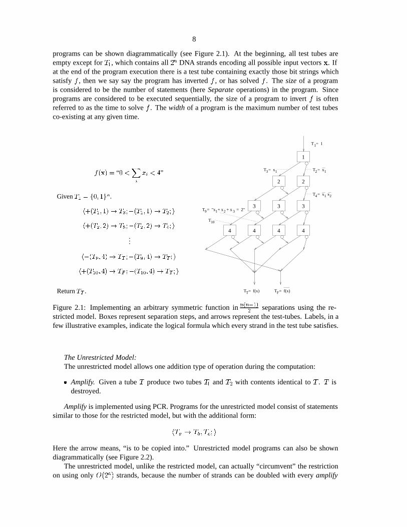
programs can be shown diagrammatically (see Figure 2.1). At the beginning, all test tubes areempty except for T1, which contains all 2n DNA strands encoding all possible input vectors x. Ifat the end of the program execution there is a test tube containing exactly those bit strings whichsatisfy f , then we say say the program has inverted f , or has solved f . The sizeof a programis considered to be the number of statements (here Separateoperations) in the program. Sinceprograms are considered to be executed sequentially, the size of a program to invert f is oftenreferred to as the time to solve f . The width of a program is the maximum number of test tubesco-existing at any given time.
f(x) = “0 <Xi
xi < 4”
Given T1 = f0; 1gn.
h+(T1; 1)! T3;�(T1; 1) ! T2; i
h+(T2; 2)! T5;�(T2; 2) ! T4; i
...
h+(T9; 4)! TT ;�(T9; 4) ! TT ; i
h+(T10; 4) ! TF ;�(T10; 4) ! TT ; i
Return TT .
1
22
333
4444
T = x
T = 1
T = x
T = f(x) T = f(x)
T = x x
1
2
T = "x + x + x = 2"2 3 1
T F
9
3
4
2
1
1 1
10T
Figure 2.1: Implementing an arbitrary symmetric function in n(n+1)2
separations using the re-stricted model. Boxes represent separation steps, and arrows represent the test-tubes. Labels, in afew illustrative examples, indicate the logical formula which every strand in the test tube satisfies.
The Unrestricted Model:The unrestricted model allows one addition type of operation during the computation:
� Amplify. Given a tube T produce two tubes T1 and T2 with contents identical to T . T isdestroyed.
Amplifyis implemented using PCR. Programs for the unrestricted model consist of statementssimilar to those for the restricted model, but with the additional form:
hTa ! Tb; Tc; i
Here the arrow means, “is to be copied into.” Unrestricted model programs can also be showndiagrammatically (see Figure 2.2).
The unrestricted model, unlike the restricted model, can actually “circumvent” the restrictionon using only O(2n) strands, because the number of strands can be doubled with every amplify

9
2
3
4
T = x
T = 1
T = x
T = f(x)
1
T
3 2 1 1
1
4
1
2 3
T IGNORE
Figure 2.2: Implementing the function f(x) = x4(x2 + x3) + x4(x1x2 + x1x3+ x3x2) using theunrestricted model.
operation. We might expect that the unrestricted model is significantly more powerful than therestricted model. Surprisingly, even though we allow the extra volume “for free”, there is littlebenefit.
The Augmented Model:The augmented model (introduced in Boneh et al. (1996b,a)) does not allow amplify, but
instead it adds a different type of operation to the restricted model. Here we make use of additionalvariables xn+1 : : : which are not assigned values by the input.
� Append[xi = v]. Given an index i > n, a tube T whose strands each encode values forvariables fxjg not including xi, and a value v 2 f0; 1g, modify every strand by ligating theDNA sequence encoding xi = v.
Programs for the augmented model consist of statements similar to those for the restrictedmodel, but with the additional form:
hTa �i; iNote that appendcannot assign a value to a variable which has already been set, and similarly werestrict separateto cases where on every strand the separation variable has been assigned a value.Only program for which this two properties can be guaranteed are considered valid. Augmentedmodel programs can also be shown diagrammatically (see Figure 2.3).
In the augmented model, like the restricted model, the number of strands remains constant at2n. Nevertheless, we will see that the augmented model is more powerful than the unrestrictedmodel, and that the unrestricted model is more powerful than the restricted model.

10
TT = f(x) FT = f(x)
2
T = 11
4
+5
1 1
3
-5+5
3 1 2
55
Figure 2.3: An augmented model program implementing a function of unknown importance.
2.2.2 Branching Programs
Since branching programs are not as familiar a model as formulas, finite-state automata, circuits,Turing machines, etc., it is worthwhile to present an exact definition here. We quote from Wegener(1987), p. 414:
A branching program (BP) is a directed acyclic graph consisting of one source(no predecessor), inner nodes of fan-out 2 labelled by Boolean variables and sinks offan-out 0 labelled by Boolean constants. The computation starts at the source whichis also an inner node. If one reaches an inner node labelled by xi, one proceeds to theleft successor, if the i-th input bit ai equals 0, and one proceeds to the right successor,if ai equals 1. The BP computes f 2 Bn6 if one reaches for the input a a sink labelledby f(a).
The size of a BP is the number of inner nodes. Many measures of BP have been studied,especially depth and width.
We follow Razborov (1991) in defining a nondeterministic branching program (NBP): weadditionally include unlabelled “guessing nodes” of fan-out 2 where both branches are allowed7.The NBP computes f 2 Bn if by some allowable path one reaches a sink labelled 1 for alla 2 f�1(1). The size of an NBP includes the guessing nodes. BP and NBP may be viewedpictorially, as in Figures 2.4 and 2.5, in which the designations “left” and “right” are replaced by“dotted-line” and “solid-line” respectively.
6Bn is the set of all n-input boolean functions.7This definition of NBP coincides exactly with Meinel’s 1-time-only nondeterministic branching programs. His
more general definitions seem not to be useful in the context of molecular computing.

11
sourcex1
x2
x3
x4
0
x3
x4
1
x2
Figure 2.4: Implementing PARITY of 4 variables using a branching program of width 2.
source
1
0
x1
x2
x3
x4x4
x5 x5
x6 x6
Figure 2.5: Implementing a function using a nondeterministic branching program. f(x) = “ x ispalindromic except for isolated (non-adjacent) errors”. NBP (f) � 2n+ 2.
We introduce one more modification of branching programs: write-once branching progams(WOBP) are branching programs where the edges may be labelled to assign a value 1 (+) or 0 (-)to any number of gate variables fgig, and where decision nodes may be labelled by a gate variableinstead of an input variable if all paths to that node assign a unique value to the gate variable.Finally, we also consider circuits where each gate has arbitrary fan-out and computes any booleanfunction of its 2 inputs.
2.2.3 Correspondence of Models
Restricted Model� Branching ProgramsIn this section we show that the class of functions which the restricted model can invert in a
given time are exactly those functions computed by a branching program of the same size.Examining Figures 2.1 and 2.4, it is clear that not much needs to be proved. The models are
essentially identical, except for interpretation. Each separation step corresponds to an inner nodeof the BP. A strand of DNA corresponds to an input vector for the BP. In summary:
1. If restricted model program P solves f in k steps, then there is a BP G which computes fand is of size k.

12
sourcex1
x2
x3x3
x2 -g1
-g1
+g1 +g1
01
g1 g1
x4x4
Figure 2.6: A small width-2 WOBP.
(a)
x3
x2
x3
Figure 2.7: A circuit for the XOR of 3 inputs.
2. If BP G computes f and is of size k, then there is a restricted model program P whichsolves f in k steps.
A single strand of DNA will flow through the test tubes of a restricted model program exactlyin the order of inner nodes executed by the associated BP running on an equivalent input vector8.Since all possible strands are run in parallel, those that end up in the output test tube TT are exactlythe inputs that the BP accepts; i.e. f�1(1).
Unrestricted Model� Nondeterministic Branching ProgramsIn this section we show that the class of functions which the unrestricted model can invert in a
given time are exactly those functions computed by a nondeterministic branching program of thesame size.
Examining Figures 2.2 and 2.5, it is clear that not much needs to be proved. We additionallyassociate amplifystatements with guessing nodes in the NBP. Just to be clear, we show:
1. If unrestricted model program P solves f in k steps, then there is a NBPG which computesf and is of size k.
2. If NBP G computes f and is of size k, then there is a unrestricted model program P whichsolves f in k steps.
8The author is reminded of some friends who needed to transfer a lot of graphics images from San Francisco to LosAngeles. They considered using FTP over the internet, but on second thought realized it would be faster to put the datain their car and drive, so they did. We are doing the same thing here: We physically move a bunch of DNA through thevirtual CPU, one gate at a time – but lots of data simultaneously.

13
We use essentially the same argument as above. However now we say that the set of test tubeswhich a DNA strand passes through is the same as the set of nodes of the NBP which could beactivated by the associated input vector. Thus the output test tube contains all strands which couldcause the NBP to accept; i.e. f�1(1).
Augmented Model�Write-Once Branching ProgramsIn this section we show that the class of functions which the augmented model can invert in a
given time are exactly those functions computed by a write-once branching program of the samesize.
Examining Figures 2.3 and 2.5, it is clear that not much needs to be proved. We additionallyassociate appendstatements with writing nodes in the WOBP. Just to be clear, we state:
1. If augmented model program P solves f in k separationsteps, then there is a WOBP G
which computes f and is of size k.
2. If WOBPG computes f and is of size k, then there is a augmented model program P whichsolves f in k separationsteps.
We use essentially the same arguments as above; the output test tube contains all strands whichcause the WOBP to accept, i.e. f�1(1), and additionally each strand maintains a record all writtenvariables.
The results of Boneh et al. (1996a) can be used to show that WOBPs are as powerful as circuits:
1. If a circuit C or size k solves f , then there is a WOBP G which computes f and is of size� 3k.
2. If WOBP G computes f and is of size k, then there is a circuit C which solves f and is ofsize k.
2.2.4 Corollaries and Conclusions
We now have a theoretical handle on precisely what can and cannot be computed by the restrictedand unrestricted models. First, by looking at the polynomial size complexity hierarchy, we canseparate the classes of functions solvable by the DNA models.
Many useful results follow immediately from the literature on branching programs. Here is abrief sampler:
� poly-size BP are equivalent to log-space non-uniform TM9 (Meinel 1989).
� poly-size NBP are equivalent to log-space non-uniform NTM (Meinel 1989).
� poly-size circuits10 are equivalent to poly-time non-uniform TM (Wegener 1987).
� thus poly-size BP � poly-size NBP � poly-size circuits, where the inclusions are believedto be proper.
� poly-size, constant-width BP are equivalent to log-depth circuits (Barrington 1986; Cai andLipton 1989).
9(N)TM = (nondeterministic) Turing machine.10In this note we consider circuits where gates are fan-in 2, arbitrary fan-out, and have arbitrary logic.

14
function fn PARITY DISTINCT MAJORITY SYMMETRIC
LAON (f) n2 O(n2 logn) O(n3:37) O(n4:37)
n2 ( n2
log n) (n2) (n log logn)
BP (f) 2n� 1 O(n log3 n) O( n2
logn)
2n� 1 ( n2
log2 n) ( n log n
log log n) ( n log n
log log n)
NBP (f) 2n� 1 O(n3=2)
( n3=2
log n) (n log log log� n)
C(f) n� 1 O(n log n) O(n) O(n)
n� 1 (n) (n) (n)
Table 2.1: Lower and upper bounds on complexities under known models for various functions.
� 3pC(f) � NBP (f) � BP (f) � L(f) (Razborov 1991)11.
� C(f)3� BP (f) � L(f) + 1 (Wegener 1987)12.
With each of these results there is typically an efficient simulation (Pudlak 1987). Otherknown linear simulations by branching programs include finite-state automata (FSA) and 2-wayfinite-state automata (Barrington 1986).
As mentioned earlier, results on polynomial equivalence are only of theoretical and not prac-tical relevance. We would like more exact bounds on the complexity of implementing specificfunctions. The literature on branching programs gives us some such bounds, although admittedlythe knowledge is very incomplete. Some known bounds13 for a few functions14 are summarizedin Table 2.1.
2.2.5 Discussion
Do we gain anything by using the amplifyoperation? Theoretically, yes, but very little. Contraryto the suggestion in Lipton (1996b), the unrestricted model does not allow us to invert functionsdefined by circuits in linear time15. Furthermore, in addition to concerns about the reliability of
11C(f) is circuit size, L(f) is AON formula size, etc. F � G means F = O(G).12Note this construction for formulas is better than that given in Lipton (1996b).13See especially Wegener (1987): pp. 76, 85, 143, 243, 247, 261, 440; Razborov (1991): pp. 50, 51; Boppana and
Sipser (1990): pp. 793-797. Note Razborov incorrectly quotes the BP lower bound on MAJORITY (Babai et al. 1990).The upper bound comes from Sinha and Thathachar (1994). The upper bound on formulas for symmetric functionsfollows directly from the upper bound Wegener gives for MAJORITY. The upper bound on circuits for DISTINCTcomes from a simple application of SORT, followed by adjacent comparisons; a better bound may be achievable. Theupper bound on NBP for symmetric functions uses a construction by Lupanov for switching-and-rectifier circuits (seeRazborov (1991)); the construction also works for NBP.
14Let jxj denote the length of x and #x denote the number of 1’s in x. Let m =n
2 log2 n; jxij = 2 log2 n and
DISTINCT(x1; : : : ;xm) = 0 iff 9i 6= j s.t. xi = xj . MAJORITY(x) = 1 iff #x � n
2where n = jxj.
PARITY(x) = 1 iff #x � 1 mod 2. f is SYMMETRIC if f depends only on #x. The lower bounds are foralmost all symmetric f .
15It appears that Lipton realized this shortly after distributing his draft. He later characterizes his constructions interms of contact networks, which are related to branching programs (Lipton 1995).

15
PCR, we should realize that each amplifyat least doubles the volume of DNA that we have to han-dle. After just a few such operations, we could practically be unable to continue the computation.For example, if we conclude for practical reasons that 250 molecules of DNA are the most we canhandle in one test tube, then we must be very careful not to exceed this limit when merging theproducts of amplification16. The augmented model of Boneh et al. (1996a), however, both avoidsthe difficulties of the amplify operation and achieves inversion of functions defined by circuits.Another model which achieves inversion of functions defined by circuits is the memory model ofAdleman (1996), which can be implemented via site-directed mutagenesis using the methods ofBeaver (1996) (who went further to show a full Turing machine simulation).
Because circuits are such a concise representation for most functions of interest, the aug-mented model seems to provide an effective way to exploit the parallelism of DNA reactions tosolve inverse problems. However, for functions represented by circuits of size 1000, the required3000 laboratory steps is still a lot to ask, especially since each affinity separation and ligation stepwould take at least an hour if performed by a competent technician according to standard proto-cols. It is not yet clear what the best biotechnology is for the separationand appendoperations,nor what their intrinsic error rates must be. Methods to improve error rates due to misclassificationduring separations (Karp et al. 1996; Roweis et al. in press) require multiplicative increases in thenumber of steps, because each separation is repeated enough times to make classification errorsrare.
2.3 0(1) Methods for DNA Computation
Abstract17 This section introduces a more novel brand of DNA-based com-puting wherein the problem to be solved is encoded entirely in the DNA se-quences used, and a fixed sequence of experiments is performed. We focus onthe experimental technique of whiplash PCR, as introduced in Hagiya et al.(in press) for DNA computation, in combination with combinatorial assem-bly PCRto generate structured libraries. We introduce a model of compu-tation based on this technique based on GOTO graphs, in which a numberof NP-complete problems can be solved in O(1) biosteps, including branch-ing program satisfiability, the independent set problem, and the Hamiltonianpath problem. In addition, we propose a simple extension of the experimentaltechnique that allows single DNA strands to simulate the execution of a feed-forward circuit, giving rise to a solution to the circuit satisfiability problem inO(1) biosteps.
In an ingenious paper, Hagiya et al. (in press) introduce an experimental technique they callpolymerization stopand theoretically show how by thermal cycling, individual DNA moleculescan compute the output of Boolean �-formulas (and-or-not formulas in which every variable is
16On a similar note, even the restricted model can solve f computed by Meinel’s more general NBP model, simply byusing 2
m times more DNA volume when there are m non-deterministic variables. This allows computation as efficientas circuits, but at the cost of ridiculous amounts of DNA.
17Results in this section also appear in Winfree (in press b). Thanks to Masanori Arita, Daisuke Kiga, KensakuSakamoto, Shigeyuki Yokoyama, and Masami Hagiya for discussions of their work; and to Len Adleman for suggestingthe HPP example and the name “whiplash PCR.”

16
referenced at most once). Because each DNA molecule repetitively forms hairpins so that it canserve simultaneously as both “primer” and “template” for a stopped polymerase reaction, Adle-man has dubbed this experimental technique whiplash PCR. Hagiya et al. (in press) describe howwhiplash PCR can be used to solve the problem of learning �-formulas given positive and negativedata, and more recently Sakamoto et al. (in press ) has shown how other NP-complete problemscan be solved with whiplash PCR18.
The motivation for whiplash PCR begins with the interpretation of DNA polymerase as an en-zymatic Turing Machine implementing the simply COPY operation. Bennett (1982) goes fartherand imagines designing a set of enzymes to simulate the operation of an arbitrary Turing Machine,but these ideas were never implemented because of the difficulty of designing enzymes de novo.But is the existing polymerase enzyme’s computational capability limited to just copying? Re-cently, Leete et al. (in press) realized that the hybridization of primers in the polymerase chainreaction (PCR) provides information-based control over the COPY operation, and that complexcomputations (such as the symbolic expansion of determinants) can be carried out in DNA usinga series of PCR reactions. However, this is a very labor-intensive series of laboratory procedures,and it has not yet been attempted experimentally. Hagiya et al. (in press) adds two key insights:(1) that polymerase copying activity (which was initiated by the primer sequence) can be conve-niently terminated by a “stop sequence” in the template DNA; and (2) that if the 30 end of a DNAstrand serves as the same strand’s primer, then an individual DNA molecule can be a self-containedcomputational unit. It was shown how in a single reaction, each DNA strand can independentlycompute the result of a �-formula, and how the problem of learning �-formulas from N positiveand negative examples can be solved in in O(N) biosteps. (We use the term “biostep” to refer to asingle laboratory procedure. Many chemical reaction steps can take place during a single biostep;in whiplash PCR, the many chemical reactions are sequenced by thermal cycling.)
The DNA used in whiplash PCR has the form 50-stop1-new1-old1- � � � -stopn-newn-oldn-head-30. When the 30 end (head) of the DNA strand anneals to a DNA sequence oldi, polymerasecopies the sequence newi, and the polymerase is stopped and dissociates upon encountering thesequence stop (for example, because the stop sequence is GGG and the polymerase buffer con-tains only A; T; and G). The head of the DNA now contains a new sequence. Upon the nextthermal cycle, the head can anneal to a different old location, and copy the corresponding newsequence. We will refer to the basic DNA unit 50-stop-new-old-30 as a frameand use the notation(new old). In general, boldface will be used when referring to DNA sequences, while italics willbe used when referring to logical variables.
We describe by example the method given in Hagiya et al. (in press) by which a single DNAstrand computes a �-formulas during whiplash PCR. Consider the �-formula f = (x1 _ x3) ^(x2 _ x4). This can be translated to the decision process shown in Figure 2.8, wherein variablex1 is checked first; if it is false (written False, 0, or �) then variable x3 is checked, etc. Decisionprocesses of this form are known as branching programs19; they have already arisen in the studyof DNA computing based on affinity separation (Winfree 1996a). Here we have the restriction thateach variable be accessed at most once; we call these �-branching programs. �-branching pro-grams can represent more functions than �-formulas; in the absence of this restriction, branchingprograms are provably more concise than formulas20.
18Sakamoto et al. (in press ) use the term successive localized polymerizationto allow for the possibility of inter-molecular reactions as well as intramolecular reactions.
19Also known as binary decision diagrams.20For example, the best known procedure for finding and-or-not formulas implementing symmetric functions results
in formulas of size O(n4:37), whereas branching programs of size O(n2
log n) can be achieved.

17
++
+-
-+
- -+
- +
-
- ++ -
(a)
out- out+
(b)
out- out+
x1
x2
x1
x2x3
x4
x4
x3
Figure 2.8: (a) A branching program for computing the �-formula (x1_x3)^(x2_x4). A possibleinput would be x1 = 1; x2 = 1; x3 = 0; x4 = 1, which leads to output +. The computationfollows a path through the diagram, and thus can only access variables in the order prescribed. (b)A branching program which does not correspond to a �-formula.
The translation of an n-variable �-branching program into DNA makes use of the 3n+2 DNAsequences fx1;x�1 ;x+1 ; � � � ;x+4 ;out�;out+g. Each edge in the diagram, say the � edge fromnode i to node j, is then converted into a DNA frame (xj x
�
i), which may be read as “if xi is False,
check xj next.” A recursive formula is given in Hagiya et al. (in press) that converts any �-formuladirectly into a sequence of DNA frames, the program frames. To tell the DNA the values of theinput variables, we use additional frames of the form (x+
ixi), read as “xi has the value True;”
these are the data frames. The data frames and the program frames are concatenated into a singlestrand of DNA, with an initial 30 head sequence complementary to x1. Figure 2.9 gives a full setof frames used to implement f and shows how the computation proceeds during whiplash PCR:the head initially anneals to the data region to read the value of x1; in the next thermal cycle, thehead anneals to the frame representing the appropriate edge out of node 1 in the program region,to determine which variable must be checked next; in the next cycle, the head anneals again to thedata region, and so on21. Because the head might anneal to its previous location (in which case thepolymerase is immediately dislodged by the stop sequence and nothing happens), the computationproceeds at approximately 1 logical step per two thermocycles. In this fashion, every DNA strandcomputes in parallel, each containing its own data and its own program.
In the inductive inference problem discussed in Hagiya et al. (in press), one starts with acombinatorial library of DNA representing all �-formulas of a given size. In each iteration, apositive or negative input example is evaluated by each DNA strand: DNA representing the inputis ligated to all remaining DNA strands, which are then evaluated in parallel using whiplash PCR.Those DNA strands computing the correct output value are retained, and the program region is cutfrom the data and head regions in preparation for the next round of the iteration. After all input
21The restriction that each variable be used at most once arises because the value of the variable itself, encoded inDNA as x�
i, is used to keep track of where the computation is in the decision diagram; if there were two nodes which
check variable i, then the computation could return to the wrong place in the diagram because there would be twoframes matching x�
i.

18
data program
(out+ x4+)
(x4+ x4)
(x4 x2+)
(x2+ x2)
(x2 x1+)
(x1+ x1)
Step 6
Step 5
Step 4
Step 3
Step 2
Step 1
(x4+ x4) (x2+ x2) (x3- x3) (x1+ x1) (out- x3+) (x2 x3- ) (out+ x4+) (out- x4-) (x4 x2+) (out+ x2-) (x2 x1+) (x3 x1-) x1
Figure 2.9: Probable secondary structures during the computation of the �-formula (x1 _ x3) ^(x2_x4) on the input 1101. “Probable” is in the mind of the artist. Note that the tick marks denotethe stop sequence; because the 30 head sequence will never contain the complement to the stopsequence, this will be the site of a small bulge in regions that are shown as double-stranded.
examples have been processed, the only DNA programs that remain represent �-formulas whichagree with all examples, and the inductive inference problem has been solved in O(N) biosteps.
By starting with a combinatorial library of DNA representing possible inputs, Sakamoto et al.(in press ) describe how whiplash PCR can also be used to solve other NP-complete problems, in-cluding conjunctive-normal-form satisfiability (CNF-SAT), Vertex Cover, Direct Sum Cover, andHamiltonian Path. In the next two sections, we develop similar results for general formula satisfia-bility (FSAT), branching program satisfiability (BP-SAT), Independent Set, and Hamiltonian Path.We suggest the assembly graphformalism for the assembly PCR technique, and the GOTO graphformalism for describing computations possible by performing assembly PCR and whiplash PCRfollowed by a single affinity separation.
2.3.1 Solving FSAT in O(1) biosteps
Even though a single strand of DNA can only compute the result of a �-formula, it is possibleto solve the formula satisfiability problem in O(1) biosteps – without the restriction that eachvariable can occur at most once.

19
Consider the Boolean formula f = (x1 _ x2) ^ (x1 _ x3): It is a function of n = 3 variables,and it accesses one of them more than once; thus it is not a �-formula. However, if we introducethe new variables x11 = x12 = x1, then the same function is computed by the �-formula f =
(x11 _ x2) ^ (x12 _ x3); with the additional constraint that x11 = x12.In general, if f is a Boolean formula in n variables in which variable i is accessed �i times,
then we can construct a �-formula f in n =P
n
i=1 �i variables, which computes the identicalfunction for input which is appropriately constrained. Specifically, for each 1 � i � n, we requirexi1 = : : : = xi�i .
We can use the biochemistry of whiplash PCR to compute the �-formula, and use the bio-chemistry of hybridization to generate a combinatorial library of DNA representing all possibleinputs which obey the equality constraints. Following Adleman (1994), the combinatorial libraryconsists of DNA representing paths through a graph. We use bipartite assembly graphs, in whichnodes are either black or white and are labelled by distinct single symbols, and directed edges arelabelled by symbol strings (possibly length zero) whose symbols are disjoint from those used atnodes. Each symbol represents a unique sequence of DNA. An oligo is generated for each edgein the graph, using the sequences for the symbols of the origin node, the edge, and the destinationnode: since the graph is bipartite, edges are either from white nodes to black nodes (in which case“sense” oligos are synthesized), or from black nodes to white nodes (in which case the Watson-Crick complementary “anti-sense” oligos are synthesized). These oligos may be mixed in a singletest tube and full-length product may be generated using assembly PCR22 (Stemmer et al. 1995).This reaction creates long “repetitive” DNA, which may then be cut at a restriction site to yielddefined-length product, and then made single-stranded. For each path through the graph, the se-quence of node and edge symbols on that path will be generated in DNA by assembly PCR; thecomplementary DNA will also be generated23. Figure 2.10 gives an assembly graph for generatingall DNA representing inputs where x11 = x12.
P0 P1 P2 P3 P0
(x+11
x11)(x+
12x12)
(x�11
x11)(x�
12x12)
(x+2x2)
(x�2x2)
(x+3x3)
(x�3x3)
Figure 2.10: An assembly graph for generating input to the formula (x1 _ x2) ^ (x1 _ x3). Up to2n + 1 oligos are required, and additional symbols Pi are used. For convenience, the node P0 iswritten twice. Since there will be a restriction site in P0, this results effectively in paths from theleftmost node to the rightmost.
Thus, for any �-formula f , we can generate a combinatorial library of DNA representing all
22This technique is preferred over annealing and ligation due to its improved yield and accuracy; it was used inOuyang et al. (1997) to create a full library of 6-bit inputs. Note that if the oligos are simply annealed, there are gaps inthe double-stranded DNA; these gaps are filled in by the polymerase during assembly PCR. If, as in Adleman (1994),ligation rather than assembly PCR is preferred, then additional oligos must be generated complementary to the frameson the “anti-sense” strands. Of course, for either ligation or assembly PCR to be effective, careful design of the oligosis required; see, for example Deaton et al. (in press).
23To be assembled by ligation, no gaps may be present in the the “sense” strand; therefore all “anti-sense” edgesmust be labelled by the empty string, or additional oligos complementary to the single-stranded “anti-sense” regionsmust be synthesized. A general assembly graph can be easily transformed into one suitable for ligation by either ofthese two modifications.

20
possible inputs satisfying the equality constraints fxi1 = : : : = xi�ig. After assembly of theinput DNA, DNA representing f can be ligated to the end of all input DNA, the whiplash PCRreaction performed, and DNA whose 30 end is out+ extracted. This DNA contains the inputwhich satisfies the original formula f . We have solved FSAT in O(1) biosteps (granting that thenumber of thermocycles necessarily will scale with the size of the formula). The exact proceduredescribed above can also be used for the slightly more difficult BP-SAT problem.
2.3.2 Combinatorial Sets of GOTO Programs
We would now like to generalize the techniques used to solve FSAT. To solve FSAT, a sequenceof three laboratory procedures was employed: combinatorial generation of DNA by assemblyPCR, evaluation of �-formulas by whiplash PCR, and selection of DNA evaluating to True byaffinity separation. Here we introduce a new formalism to describe the computations which canbe performed in this manner; this formalism suggests several optimizations and new applicationsof whiplash PCR.
Our interest comes from the following simple observation: On a given strand of properlyconstructed DNA, whiplash PCR can be considered as executing a BASIC program consistingentirely of GOTO statements: e.g. the DNA frame (xj xi) can be thought of as “Line i: GOTOline j”, or just i ! j. The special “line numbers” are START = 1, ACCEPT = out+ andREJECT = out�. The sequential order in which the GOTO statements appears does not matter,but no line number may appear on the left hand side twice. By using combinatorial synthesis tocreate a huge number of different programs, and extracting the accepting ones, we are able tosolve some interesting mathematical problems. We define a combinatorial set of GOTO programsusing a bipartite assembly graph where edges are labelled (possibly with repetition) by GOTOstatements and nodes are labelled (uniquely) from Pi. We will insist that all paths generate validGOTO programs, in which no line number appears twice on the left hand side24. This implies,among other things, that the graph has no cycles.
Thus, we consider the following question: Given a graph as defined above, is there a path thatgenerates a GOTO program that reaches ACCEPT when started at line 1? Call this the GOTOgraph satisfaction problem, or GG-SAT. GG-SAT thus formalizes what can be computed in O(1)biosteps by applying assembly PCR followed by whiplash PCR and affinity separation.
As an example, we will reduce BP-SAT to GG-SAT. Three resource measures of importanceare the number of paths through the graph (corresponding to the number of DNA strands gener-ated); the maximal length of the GOTO programs thus generated (corresponding to the length ofthe DNA strands); and the size, in number of edges, of the GOTO graph (corresponding to thenumber of DNA oligos that must be synthesized). Then, as shown in Figure 2.11(a), n-variablem-node BP-SAT can be solved by creating 2n programs of length 2m + n, using a GOTO graphof size 2(n+m). m lines of the program are fixed; the other m lines are generated in independentblocks of �i lines, with two possibilities for each.
This notation makes it obvious that the fixed portion of a GOTO graph is redundant; we canreduce each graph to a smaller one by following all the GOTOs in the fixed portion. The examplein Figure 2.11(a) reduces to just 3 nodes as shown in Figure 2.11(b). Thus we get the improvedtheorem that n-variable m-node BP-SAT can be solved by creating 2n programs of length m
using a GOTO graph of size 2n. The m lines are generated in independent blocks of �i lines, withtwo possibilities for each. Because this decreases both the length of the DNA and the number
24DNA programs in which a line number appears more than once on the left hand side would executeprobabilistically.

21
(a)
input regionz }| {program regionz }| {1!6
1!7
2!8; 3!10
2!9; 3!11
4!12; 5!14
4!13; 5!15
6!2 7!3 8!5 9!4 10!4 11!5 12!� 13!+ 14!+ 15!�
(b) combined input and program regionz }| {1!2
1!3
2!5; 3!4
2!4; 3!5
4!�; 5!+
4!�; 5!+
Figure 2.11: Reducing BP-SAT to GG-SAT: the n = 3; n = 5 example. (a) The directconstruction, combining the assembly graph from Figure 2.10 and the �-formula program for(x11 _ x2)^ (x12 _ x3). (b) The optimized construction obtained by following GOTO statementsin the fixed region of (a). All GOTO programs are of length 5.
of cycles to complete the program, this construction could be important for experiments solvingBP-SAT. It would be interesting to find general polynomial-time algorithms for “optimizing” or“compressing” arbitrary GOTO graphs, in the sense that the new graph solves the same problembut contains fewer paths and/or shorter programs.
0
1
0
1
0
1
0
1
0
1 1
0
1
0
1
0
1
0
1
0
1 1
0
1
0
1
0
1
0
1
0
1 1
0 0 0 0 0
program regionz }| {input regionz }| {
|
{z
}
count1's
x1 x2 x3 x4 x5 x6 x7 x8
Figure 2.12: A GOTO graph for solving the Independent Set Problem. Inputs are generated inwhich exactly k = 3 out of n = 8 variables have value 1. The edge labels “0” and “1” in columni are shorthand for GOTO statements setting the value of variable xi; as in FSAT, variables whichare referenced more than once in the formula must be duplicated, and the corresponding edges inthe graph will be labelled with more than one GOTO statement. Note that concentration ratios ofthe oligos could be adjusted to make all paths equally likely (for ligation-based assembly, at least;it is not so clear for assembly PCR).
However, we are still failing to fully exploit the expressive power of the graph; so far wehave considered only essentially linear graphs. In the context of circuit satisfiability, Bonehet al. (1996a) commented that providing a regular language as input to the circuit, rather than

22
just f0; 1g� , could for some problems both reduce the size of the circuit and decrease the vol-ume of DNA needed to solve the problem, and that the desired n-bit input can be provided byassembling DNA paths through a graph of size nM , where M is the size of a finite state machinerecognizing the regular language. The same comment holds true for BP-SAT. A simple exam-ple follows from the ideas in Bach et al. (1996): the polynomial time 2SAT problem becomesNP-complete when given the restriction that satisfying solutions must have exactly k ones. Aninstance is the Independent Set Problem, which asks, given an undirected graph and an integer k,is there a subset of k vertices which have no edges among themselves? The 2-CNF formula wewill use for this problem is
^es=1(xis _ xjs)where the graph has edges [i1; j1] : : : [ie; je] and xi indicates membership in the independent set.The formula simply checks that no two chosen vertices have an edge between them. To solve theproblem, we ask for a solution to this formula in which exactlyk variables are 1. This is done inDNA by generating only inputs with k variables set. A GOTO graph for this problem is shown inFigure 2.12; variables used more than once must be duplicated, and the fixed GOTO statements inthe “program region” can be eliminated just as in the BP-SAT optimization.
P i 1
������������
������������
����������������
������������
������������
������������
������������
������������
������������
������������
������������
1
2
3
4
5 6
7
1 2
5
3
4
6 5
4
2
3
6
7
2
5
32
4
4
6
3
2
1 2
1 2
4 5
4 5
2 3
2 3
2 3
2 3
5 65 6
3 4
3 4
3 4
3 45 6
2 3
5 6
4 5
2 3
4 5
6 7
6 7
6 7
3 4
3 42 3
5
6
4 5
5 6
4 56 7
3 4
2
3
P i P i P i P i P i P i2 3 4 5 6 7
(b)(a)
Figure 2.13: Solving the Hamiltonian Path Problem: A graph G (a) and its corresponding GOTOgraph GG (b). This is Adleman’s example with 2 additional edges added to prevent pruning fromsimplifying the GOTO graph to triviality. For convenience the nodes show only the vertex indexi, and not the full symbol Pik .
As a final example, we consider the Hamiltonian Path Problem (HPP) solved in Adleman(1994). Our procedure begins by converting (in polynomial time) the original graph G into aGOTO graph GG. Suppose G has n vertices; then GG will have n2 vertices, arranged in layers,such that if there is an edge [i; j] in G, then in the GOTO graph, for each k 2 f2 � � � ng there isan edge [Pik�1 ; Pjk ], labelled i ! (i + 1) (with ACCEPT = n). Since we are only interestedin paths from vertex 1 to vertex n, we prune the new graph to include only vertices which maybe reached from P11 and which may reach Pnn ; this dynamic programming problem takes timeO(n2) on an electronic computer. We now have the GOTO graph GG, as shown in Figure 2.13. IfG has E edges, then GG requires less than E2 oligos.
Every path through GG represents a length n path through G from vertex 1 to vertex n. AHamiltonian path will contain, in some order, the frames
f1! 2; 2! 3; � � � ; (n� 1)! ACCEPTg;

23
and thus the GOTO program, as executed by whiplash PCR, will proceed to ACCEPT . All otherpaths will duplicate some frame and lack another – these GOTO programs will terminate andnever reach ACCEPT . Consequently, extraction of DNA containing the ACCEPT sequencewill identify the Hamiltonian path, and we have solved HPP in O(1) steps.
2.3.3 Single-Strand Computation of Boolean Circuits
Using whiplash PCR in the manner suggested in Hagiya et al. (in press), where exactly one symbolis copied in each polymerization stop step, gives each strand exactly the computational power of aGOTO program, and no more. However, whiplash PCR may give each strand more computationalpower, if copying more than one symbol is experimentally feasible. The idea is this: when thehead of the DNA strand is being extended, it might not only change the “state” of the head butalso add a new “program” frame.
Suppose for the moment that the variables xi are encoded by xi;x+
i;x�
iusing A, T, and C,
and that the new gatevariables gi are encoded by gi;g+
i;g�
iusing exclusively A and T . G and C
are respectively used for representing the stop sequence and its complement. The polymerizationbuffer still includes A, T , and G, but not C . The restricted alphabet used for the gate symbolsmakes designing DNA sequences a more difficult task25, but it is necessary for the constructionwe give below because now a gate symbol can be copied by polymerase twice during whiplashPCR.
In our original discussion of branching programs, a + edge from the node reading x7 tothe node reading x4 would be encoded by the frame (x4 x
+7 ). During biochemical execution
with whiplash PCR, a transition through this edge would entail hairpin formation with bindingto x+7 and polymerase extension copying x4, as shown in Figure 2.14(a). Our new proposalinvolves copying more than x4 during the polymerase extension, thereby memorizing an interme-diate result of the computation. In Figure 2.14(b) we show the execution of an enhanced frame(x4 (g
+8 g8) (g
�
5 g5) x+7 ). Here, the original DNA encodes for the “anti-sense” of a valid frame,
and thus the frame is inactive, or hidden. The two hidden frames present here are intended toassign values to new variables g5 and g8, but that assignment will not become effective while theframe is still hidden. However, if the enhanced frame is executed, the hidden frames are copied as“sense” frames onto the growing 30 end of the DNA, thus activating the hidden frames for potentialfuture use. The final 30 sequence of the DNA will still be x4, which will determine the immediatecourse of the computation as usual.
At subsequent points in the evaluation, reference can be made to look for the values of g5 org8. These values will be found by the head hybridizing to the newly activated frames and copyingto the GGG stop sequence – only now the head will not be hybridizing to the “input” part of theDNA, but to part of the growing “head history” itself.
What is the use of activating hidden frames? The possibility of memorizing intermediate re-sults gives rise to a model of computation that we call write-once branching programs(WOBP)26.Each node still has two outgoing edges, one labeled + and the other �; however, edges may nowalso have the additional labels �gi, which indicate that the variable gi is to be assigned the value
25An expanded DNA alphabet, making use of artificial base pairs which are both highly specific and can be incorpo-rated by DNA polymerase, would allow greater flexibility in sequence design; indeed, Sakamoto et al. (in press ) reportspreliminary studies of using iso-C and iso-G (Switzer et al. 1993) in whiplash PCR. If this chemistry is successful, thevariables xi and gi could be encoded using A, T , C, and G; the stop sequence could be iso-G-iso-G-iso-G and itscomplement iso-C-iso-C-iso-C; and the polymerization buffer could contain A, T , C, G, and iso-G.
26This model can also be used to describe DNA computation performed by a sequence of affinity separations andligations, as in Boneh et al. (1996a).

24
(a)
GGG GGG GGG
x4 x+7
(b)
GGG CCC CCC GGG
x4
g8
g+
8g5
g�
5x+
7
g8
g+
8g5
g�
5
GGG GGG
+ x7
x4
+ x7
x4
+g8-g5
Figure 2.14: (a) The polymerization stop step on a standard frame, where a single symbol iscopied, and its representation as an edge in a BP. (b) The polymerization stop step on an enhancedframe, where two hidden frames are made active, and its representation as an edge in a WOBP.
+ or �. For implementation using whiplash PCR, a restriction is imposed: again, a given variablemay be read at most once, and nodes may be labeled to read any input variable xi or any gate vari-able gi, so long as all paths to a given node have assigned exactly one value to the gate variablebeing read27. We call these restricted programs �-WOBP.
+ -
-g1
-g2+g2
+g3 -g3
x1
+g1 -+
-++g5
+g6
-g5-g6
-g6-g5x3
x2
(b)
x2
x3
x1
(a)
Figure 2.15: (a) Input variables with multiple fan-out are handled by reading them once, and writ-ing multiple distinct gate variables which may subsequently be read once each. (b) The translationof a gate with fan-out 2 into a write-once branching program requires two decision nodes (onlyone of which is guaranteed to be used). Two new gate variables are written. To translate an en-tire circuit, first the input variables and then the gates would be processed in linear order in thebranching program. Clearly, much more efficient translations are possible; for example, gates withfan-out 1 need not be memorized.
�-WOBP are at least as concise as circuits28; a circuit with n inputs accessed in total n times,and g gates with total gate fan-out p can be implemented in a �-WOBP using no more than n+2g
nodes and n + p gate variables29. The simple construction uses the building blocks shown in
27Again, we have a probabilistic model if this restriction is violated.28The converse is also true: a circuit can be constructed in which (usually) two gates are used for each edge in the
WOBP to test if the edge was traversed during computation. Thus a circuit with 3m gates can be constructed from aWOBP with m nodes.
29Just 2g nodes and p gate variables are required if we allow preparing the input with duplicated variables, as in theFSAT construction.

25
Figure 2.15. First, each input variable xi is read and duplicated into �i new variables, so everysubsequent read uses a unique variable. Then, each circuit gate is processed in turn, and its outputis stored in a new gate variable (or variables, if the gate has fanout greater than unity). Thetranslation of a small circuit is shown in Figure 2.16. Thus, we can theoretically solve the circuit-SAT problem in “one pot” using whiplash PCR.
In the case shown in Figure 2.16, a much smaller �-WOBP (essentially a BP) exists whichcomputes the same function, pointing out that our construction of a �-WOBP from a circuit isnot the most efficient construction possible. However, for more difficult problems, circuits can bemuch more efficient than branching programs30. This means that a fixed size CSAT problem maybe more difficult than a BP-SAT problem of the same size.
One serious concern is that the problem of secondary structure interfering with the progressof the computation is made worse. First, “inopportune” hybridization now involves much longersubsequences, resulting in many thermocycles in which no progress is made. Secondly, newlyactivated frames are located in the “head history” region of the DNA, which is likely to be involvedin secondary structure. Experimental investigation is required to see how serious the problems willbe.
2.3.4 Conclusions and Future Directions
Like other forms of DNA computation, it seems that whiplash PCR can’t by itself compete withelectronic circuits unless there are significant advances in the control of the biochemistry. How-ever, the computational power of whiplash PCR – in theory – suggests that “one-pot” biochemicalreactions have more potential for computation than previously thought. Conceivably, whiplashPCR could be combined with other kinds of DNA processing – either stepwise or within the “onepot” biochemical reaction. For example, we can consider modifications of whiplash PCR whereinDNA strands not only grow though polymerization, but also shrink due to other enzyme activity(e.g. restriction endonucleases or topoisomerases). An open theoretical question is how to usenon-determinism during whiplash PCR: we have already discussed the case where the solution toa problem is found by first using nondeterministic steps in the generation of the DNA, and thenusing deterministic steps during the execution of the program, but whiplash PCR could equallywell be used to perform nondeterministic steps by having multiple frames matching the currenthead state.
30As a simple example, an arbitrary symmetric function can be implemented in a circuit of size O(n), but the best
construction for branching programs requires O(n2
log n) nodes.

26
(a)
x3
x2
x3
-
-
-
-
-
-
-
-+
out+ out-
+
-g7
+
+
g4+g8
+g8-g8
-
-+
g7
g8-g9
+g9
-g9
+g10
-g10-g10
-
-+
+
+
+
g9
g5+g11
+g11
-g11
+
g10
g6+g12
+g12
-g12g11
g12
+ -
+ -
+g1 -g1
-g2+g2
x1
+ -
+g3
+g4
-g3
-g4
+g5
+g6
-g5
-g6
x2
x3
g1
g3
+
+ +g7
+g7
g2
(b)
-
-
--
-
+ -
+ -
+g1 -g1
-g2+g2
+g3
+g4
-g3
-g4
x2
x3
x1
+
+
+ +
+
out+ out-
g2
g3
g1
g4
(c)
Figure 2.16: The translation of a 3 input, 6 gate XOR circuit into a �-WOBP. (a) the circuit, (b)the �-WOBP generated by our construction, (c) a much simpler �-WOBP generated by hand.

27
Chapter 3 Models of Computation by Self-Assembly
3.1 2D Self-Assembly for Computation
Abstract1 This section informally explores the power of annealing and lig-ation for DNA computation. (The following two sections will explore thesenotions more formally.) The first step of Adleman’s molecular solution to theHamiltonian Path Problem involves the creation of a combinatorial library ofDNA by means of directed self-assembly, followed by ligation. Experimen-tally, DNA annealing can produce many unusual structures in addition to theusual B-form double helix, so we wonder if they can be used to advantagefor computation. We conclude, in fact, that annealing and ligation alone aretheoretically capable of universal computation.
When Adleman introduced the paradigm of using DNA to solve combinatorial problems Adle-man (1994), his computational scheme involved two distinct stages. To solve the directed Hamilto-nian path problem, he first mixed together in a test tube a carefully designed set of DNA oligonu-cleotide “building blocks”, which anneal to each other and are ligated to create long strands ofDNA representing paths through the given graph. After this ligation stage, there ensue n stepsof affinity purification, whereby exactly the strands representing Hamiltonian paths are separatedinto a test tube (“the answer”).
Lipton (1995) subsequently refined the formalism for DNA-based computation. He did awaywith Adleman’s first stage, ligation, and replaced it by starting all computations with a fixed setof DNA strands representing all n-bit strings. Lipton expanded on Adleman’s second stage, sep-aration, where he showed how all solutions to a given boolean formula f can be separated into atest tube (“the answer”). The cost for the generality of this method, even when using the improve-ments of Boneh et al. (1996a), is indicated by considering solving the Hamiltonian path problem:a straightforward method2 takes about n3 separation steps using Lipton’s approach, compared tothe n steps used by Adleman.
We can conclude from this circumstantial evidence that much of the physical computationalpower Adleman was exploiting was in his first stage, where annealing and ligation were used.Lipton has explored the power of generalizing Adleman’s second stage; we would like now to
1Results in this section also appear in Winfree (1996b). Thanks to Paul W. K. Rothemund for the discussions atthe Red Door Cafe that lead to this work, and to Nadrian C. Seeman for suggesting the use of the double-crossovermolecule.
2Let the graph have n vertices and e edges; e � n2. The best boolean circuit I could devise uses O(en log n)
gates to verify a Hamiltonian path. Another issue is that Adleman’s ligation stage requires the synthesis of aboutO(n+ e) oligonucleotides, which is O(n2) if e = O(n2); whereas Lipton needs only about 4n log n oligonucleotidesto create his standard initial test tube of DNA. However, technology is becoming readily available for synthesizingmany oligonucleotides in parallel very quickly (see e.g.Chetverin and Kramer (1994)); the same cannot be said for theaffinity purification steps, which will likely remain expensive. Comparing volume for a graph with n=2 edges out ofeach vertex, Adleman’s method uses volume roughly proportional to (
n
2)n, while Lipton’s method uses a volume of
2n log n, since it takes n log n input variable bits to specify a potential path.

28
explore the power of generalizing Adleman’s first stage.An immediate stumbling block is that the chemistry of annealing is not fully understood. At
best we can try to define some conditions under which the reactions are predictable, or at leastunder which it is reasonable to expect that the reactions could be made to be predictable.
3.1.1 Some Basic Annealing Reactions
The fundamental chemistry of DNA is based on the double helix and the principle of complemen-tarity. Each strand of DNA is a covalently linked polymer, where each unit consists of a constantpart (the sugar-phosphate “backbone”) and one of either adenine, thymine, cytosine, or guanine(the bases A, T, C, G). Each strand is oriented; it has a 3’ and a 5’ end. When DNA forms adouble-stranded helix, the strands must be anti-parallel, and complementary bases align (A withT, C with G); such strands are called Watson-Crick complementary sequences. DNA also takes onmore complicated configurations, including triple helix, quad helix, super-coiled, and branched.
A surprising number of possibilities are available, some of which one may want, and manyof which one may not want. DNA is a particularly easy molecule to work with, because it hasevolved to be stable, typically unreactive, yet manipulable. RNA and protein, which have evolvedto serve many enzymatic functions, are far more reactive, and thus it is less easy to predict hownovel designs will behave in an experiment.
I will now comment on some reactions we may wish to exploit, presented in cartoon fashion(Figure 3.1). I will have to be more detailed with the reactions involved in the main thrust of thispaper, where their computation-universality is demonstrated.
(A) This is the canonical annealing reaction for DNA. Two strands with complementary sub-sequences will form hydrogen bonds and hybridize at the matching base pairs. The rateconstants for this reaction, which is reversible, depend on the temperature and salt concen-trations, among other things. The melting temperature, above which the complex is notstable, depends upon the number of matching base pairs.
(B) A special case of the above, where the matched region occurs at the ends. Note that the two“sticky ends” (unmatched sequences) are available for further reactions with more DNA.
(C) The above reaction can be used to join two double-stranded DNA molecules with comple-mentary sticky ends. If ligase is present in the solution, the nicks in the backbone of theproduct will be repaired by the formation of a covalent bond, resulting in two continuousstrands.
(D) If mismatches occur flanked by matching regions, the unmatched DNA can bubble out.
(E) As above, except that the mismatch occurs here on both sides. Whether this structure isstable depends critically on the temperature and concentration of salts. For example, a ruleof thumb is that the difference in melting temperature between a perfectly matched structureand an imperfectly matched structure is 1 degree per 1% mismatch (Wetmur 1991).
(F) This is the simplest DNA branched junction. The assembly of these structures consistsof course of sequential steps; only the end product is shown. This 3-armed junction isprobably floppy. However, how floppy it is depends upon the exact sequence of base pairsin the oligonucleotides.

29
(G) This 4-armed junction is commonly known as a Holliday junction. The two horizontalstrands tend not to be parallel, but skew. If the sequences along both strands are homologous,then a phenomenon called branch migration can occur, in which the crossover point driftsright or left.
(H) This is the most complicated structure we will consider. We will put it to good use later. Ithas been found to be fairly rigid and planar (Fu and Seeman 1993). Note the sticky ends.Other related double-crossover junctions are possible, depending upon the number of half-turns present in the helical regions. Seeman calls this molecule “DAE” for double-crossover,antiparallel helical strands, even number of half-turns between crossovers. “DAO”, with anodd number of half-turns between the crossovers, has an interesting topological difference:It consists of only 4 strands.
(A)S
S
(B)S
S
(C)
S
S
(D)
A B
A B
(E)
A B
A B
(F)
AB
C
A
C
B
(G)
AB
A
C
D
DB
C
(H)
F
D
E
BC
A
C
D
F
A
B E
Figure 3.1: Some basic types of annealing reaction. Curves represent single strands of DNAoligonucleotide. The half arrow-head represents the 3’ end of the strand. Small lines betweenstrands represent hydrogen bonds joining the strands. The helical structure of the DNA is notrepresented visually. Letters signify sequence motifs. A bar above a letter signifies the Watson-Crick complement of the motif.

30
All of the structures above have been made in the lab and their structures verified (see, forexample, Fu and Seeman (1993)).
We would ultimately like a theory which could tell us, given a set of oligos, a temperature,and salt concentrations, what stable structures will form, as well as the kinetics. But this is a verycomplex task!
3.1.2 Operations Using Linear DNA
We will first briefly consider what computations can be performed using annealing and ligationof strictly linear DNA molecules. Many of the possibilities have already been discussed by otherauthors. For example, the techniques used by Adleman (1994) allow for the construction of allDNA representing strings accepted by a finite-state automata (also known as a regular language),using the annealing reactions (B) and (C) above. This is important, because it allows us to createa well-defined, somewhat interesting set of inputs on which to compute in parallel. Beaver (1996)has discussed how, in conjunction with polymerase, reactions (D) and (E) can be used to makecopies of DNA with context-sensitive insertion, deletion, and replacement of substrings. In lightof these powerful operations, it seems plausible that a “one-pot” linear DNA reaction could bedesigned which performs universal computation.
3.1.3 Operations Using Branched DNA
There are many possibilities for computation using branched DNA. However, since the generalchemistry is not well understood, we will try to avoid ungrounded speculation by focusing on oneconcrete possibility. The rest of this section3 will concentrate on how to assemble a large “weave”of branched DNA which simulates the operation of a one-dimensional cellular automaton.
Background: Blocked Cellular Automata
This section develops a formal model of computation called blocked cellular automata (BCA)4.We will later show how BCA can be simulated by DNA.
The operation of a BCA is diagrammed in Figure 3.2. As in the Turing Machine model,information is stored in an infinite one-dimensional tape, where each cell contains one of a finiteset of symbols. The computation proceeds in steps, where in each step the entire tape is translated,according to a given rule table, into a new tape. The translation occurs locally and in parallel;pairs of two cells are read, and which two symbols are written is governed by look-up in a ruletable5. It is of critical importance that the reading frame (which cells are paired together) strictlyalternates from step to step.
The set of entries f(x; y) ! (u; v)g is called the rule table, or the program, of the BCA. Byappropriately designing the rule table, the BCA can be made to perform useful computation. Infact, BCA are computationally universal. A BCA with k+3s symbols can simulate in linear timethe operation of a Turing Machine with k tape symbols and s head states – the proof is analogous tothat in Lindgren and Nordahl (1990). Thus we can conclude that a BCA can be used to answer any
3The inspiration for this approach comes from the proof of the undecidability of the Tiling Problem (see Grunbaumand Shephard (1986), Chapter 11).
4BCA (Wolfram 1994) are also known as partitioning CA (Margolus 1984) and as 2-body CA or particle machines.They generalize the lattice gas model (Hardy et al. 1976), and are commonly studied in two dimensions.
5If the table contains multiple entries for a given pair of read symbols, then the BCA is said to be nondeterministic.

31
x y
g(x,y)f(x,y)
t
t+1
t+2
t+3
Figure 3.2: Operation of a BCA. The tape of a BCA, divided into cells, is shown at the bottomright. Each cell contains one of three symbols: blank, black dot, or white dot. The tapes atsuccessive time steps are stacked vertically above the initial tape. The inset, left, details the formof a rule table entry, which governs how new tapes are created.
question which can be phrased in terms of a computer program. Small BCA have been designedwhich sort lists of integers, compute primes, and many other tasks.
A few more comments are in order concerning the abstract model of blocked cellular automata.First we consider the finite-size case. In any attempted implementation of a BCA, we cannotactually construct an infinite tape. Thus boundary conditions become important. We consider thefollowing cases:
(a) No update of boundaries. We start with a finite tape of length 2n; at each step the tapebecome 2 cells shorter; and after n steps the computation can proceed no further. This caseis not universal.
(b) Inactive boundary conditions. Whenever there is an unpaired cell at either end of the tape,it is copied verbatim onto the new tape. The tape remains always the same size (n cells),and thus there are only kn possible tapes. As the computation must begin to cycle after kn
steps, this case is also not universal.
(c) Periodic initial conditions. On either side of the input cells we specify a repeating patternof symbols. Starting with just one copy of the periodic block on either side of the input,computation proceeds as in (a), but if the tape gets too short, we add another copy of theperiodic block to either side of the input tape and start the computation anew6. This case isuniversal.
(d) Self-regulated boundary conditions. Depending upon what symbol is in the boundary cell,the new tape will either shrink (as in (a)) or expand by appending a new cell to the end ofthe tape. This case is also universal.
Finally, a word on how an answer is obtained from the BCA. This is a matter of convention.Typically, when the computation is done, the answer is written on the final tape. But how is itknown when the computation is done? One possibility is that the tape stops changing; the systemhas reached a fixed-point. However in this paper we will consider that a computation is done whena special symbol, called the halting symbol, has been written for the first time anywhere on thetape.
6By memorizing boundary cells, we can avoid re-computing any cells and make the computation more efficient.

32
Simulation of BCA by DNA
We will now show how to use DNA to construct a BCA. In this section we will optimisticallyshow what chemical reactions we hopewill occur; in the following section we consider potentialdifficulties in finding conditions such that they will in fact occur as we have described.
The DNA representation of the BCA tape is a little counter-intuitive, so we will explain byexample. Figure 3.3 shows part of the DNA molecule encoding the initial tape (the input to thecomputation). To each tape symbol corresponds a short oligonucleotide sequence, which appearsin the initial molecule as a sticky end overhang in the appropriate positions. The rest of the DNA ineach segment does not vary with content, and is chosen to maximize structural stability. Note thatthe reading frame is implicit in the structural form of the DNA. Although Figure 3.3 is schematic,the 2D picture is meant to imply that the whole DNA complex is roughly planar. This is critical,and luckily, it is physically plausible.
C
DNA:
A A C
B C A
BCA:
A A C
B A
Figure 3.3: Encoding the initial tape in a DNA molecule. The sequence of sticky ends in the initialmolecule encodes the initial tape of the BCA. Thus ‘A’ denotes a symbol in the BCA diagram,whereas in the DNA diagram it denotes the unique sequence of bases associated with that symbol.
There are a variety of ways to make the initial molecule. Note that the initial molecule canbe thought of as consisting of several double crossover junctions (from Figure 3.1H, with themodification that the top and bottom strands are made to be an odd number of half-turns in length– see Figure 3.6 for detail) linked together by pieces of linear helical DNA. The sticky ends canbe designed such that only this unique molecule will self-assemble7. Ligase can be added to makethe segments of the initial molecule covalently bonded.
We will now explain how the program, that is the rule table, of the BCA is represented in DNA.For each rule, e.g. (x; y) ! (u; v), we create a double crossover molecule whose sticky ends onone helix are x and y, and on the other helix u and v8 (see Figure 3.6). All such rule molecules areadded to the solution containing the initial molecule. As shown in Figure 3.4, what is required forcomputation is that rule molecules will anneal into position if and only if both sticky ends match.
Eventually, a triangular lattice of linked DNA will form, simulating a triangular region of aBCA corresponding to boundary conditions (a) or (c) in Section 3.1.3 above (see Figure 3.5).Boundary conditions (b) and (d) can be simulated by using special rule molecules for the edge ofthe lattice; the details are not presented here. Note that each level of the lattice has a single strand
7It is easy to see that sticky end sequences can be chosen, using the same techniques as Adleman (see Section 3.1.2),such that a periodic initial molecule will form, creating periodic initial conditions as mentioned in Section 3.1.3 (c)above. Similarly, a regular language of inputs could be made in parallel.
8The lengths of all parts of the rule molecules are chosen to be constant for simplicity, but it is conceivable that byusing variable length as well as sequence to encode symbols, greater specificity could be achieved.

33
AB C
B C
B
B C
A A C
C B
A C AC A
A
C B
BC
B
CA
A C
C B
A A
AA
Figure 3.4: Rule table molecules assemble into the lattice. We see free-floating rule tablemolecules above and the initial molecule at the bottom (both correspond to the BCA in Figure 3.2).A rule table molecule, with sticky ends B and C, is about to anneal to the initial molecule. At theleft, a rule molecule which matches only at A will ultimately not stick. Note that the rule moleculewith sticky ends A and A will also not stick, because the orientation of its strands is wrong; thisrule molecule will be useful on alternate levels of the lattice.
of DNA which travels the entire length of the lattice at that level, and where the coded symbolsoccur in the sequence in in which they occur in the BCA at time t.
Level 3
Level 0
Level 1
Level 2
Level t
Figure 3.5: The DNA lattice resulting from a finite initial molecule. At the chosen annealing tem-perature, which is above the melting temperature for s base-pair annealing but below the meltingtemperature for 2s base-pair annealing, no more rule molecules can stably attach to this structure.However, if the bottom level (the initial molecule) were extended, then a larger triangle couldform. s is the length of the sticky ends in the rule molecules.
Finally we ask, how can we access the output of the computation? This breaks down into twoquestions: How do we know whenthe computation is done? And whatis on the tape at that point?There are many possible approaches to take; here we will merely sketch one. As mentioned above,we will consider the computation to be done when a special halting symbol is written on the tape9.In DNA, this corresponds to the special sticky end motif being incorporated into the lattice. Whenthis occurs, the motif will be present as a double-stranded molecule for the first time, and this site
9At this point other parts of the tape will typically “not know” that the computation is done, so the lattice willcontinue to grow. However, it is also possible to design the cellular automaton such that all cells go into a special stateto halt computation at the same time (the Firing Squad Problem, see e.g.Yunes (1994)), thereby allowing us to designlinear pieces of DNA which fit into the gaps at the final level of the lattice, so that it cannot grow further. This maymake extraction of the final tape configuration easier.

34
can be be chosen as the recognition domain for a binding protein10, which could, for example,subsequently catalyze a phosphorescent reaction, turning the solution blue. To determine what is“on the tape” at this point, it is necessary to extract the single strand of DNA corresponding to thefinal level of the BCA. To do this, first add ligase to covalently bond all the annealed segments11.Then add resolvase to break all the crossover junctions12. Finally, heat to separate the strands, anduse affinity purification to extract the strand containing the halting motif. Amplify and sequencethat strand however you desire (e.g.via PCR and standard sequencing gels).
To summarize the model suggested here, a computation would proceed as follows.
1. First, express your problem via computer program. Convert that program into a (possiblynondeterministic) blocked cellular automaton.
2. Create small molecules (H-shaped and linear) which self-assemble to create the initialmolecule (or initial molecules, if search over a FSA-generated set of strings is desired).Add ligase to strengthen the molecule.
3. Create small H-shaped molecules encoding the rule table for your program.
4. Mix the molecules created in steps 2 and 3 together in a test tube, and keep under preciseconditions (temperature, salt concentrations) as the DNA lattice crystallizes.
5. When the solution turns blue, ligate, cut the crossovers, and extract the strand with thehalting symbol.
6. Sequence the answer.
Analysis and Estimates. Will it work?
Let’s begin the analysis optimistically. The above construction is just one implementation possiblein a general class that might be called “crystal computation”13. In this class, we design a systemwhere we can tailor-make the energy (and hence free energy) as a function of the configuration.We design it such that the lowest energy state (or in our case, the lowest free-energy state at agiven temperature) uniquely represents the answer to our computation. This is closely relatedto the approach taken by Hopfield (1982) in his seminal work on neural networks. In our casethe lowest energy configuration is one where every rule molecule has all four sticky ends bound.Given the presence of the initial molecule, this can only occur if the computation proceeds asdesired.
The above analysis is a simplification that fails to take into consideration many aspects of theproposed implementation. For example, it completely ignores the dynamics involved; one simplyanneals at a slow enough schedule, the argument goes, and the crystal is the result. Whereas in
10The protein must have an active bound form, and inactive unbound form. Furthermore, we must be sure it doesn’tbind to rule molecules in the solution.
11It is a valid concern that ligase may not be able to bind to any but the outermost strands in a lattice. It may be betterto reverse the order of the ligase and resolvase steps.
12Although a resolvase has been shown to cut crossovers in double-crossover molecules (Fu et al. 1994), it is un-known whether the enzyme will be functional on the inner strands in the lattice. However, the enzyme may be able to,at diminished speed, work from the edges in.
13It has been suggested that we shouldn’t use the term “crystal”, because it has a well-defined special meaning. Atbest, our constructions yield “pseudo-crystals”, because any useful computation is aperiodic. We beg the reader to giveus slack in using this term.
35
fact the crystallization proceeds at the edges only, according to kinetics that significantly influencethe result.
Can a temperature be found such that two sticky ends bound is stable, while one sticky endbound is unstable? In other words, let T0, T1, and T2 be the melting temperatures for a rulemolecule fitting into a lattice slot where respectively 0, 1, and 2 of the sticky end pairings match.We want to keep the test tube at a temperature T such that T0 < T1 < T < T2. This shouldbe possible, but how large is the difference between T1 and T2? Although this is unknown forthe particular molecules we use, we can get some idea by looking at what’s known about linearDNA annealing. For example, under standard conditions 20 base-pair oligonucleotides (repre-senting rule molecules with two length 10 sticky ends bound) melt at 70� C, while 14 base-pairoligonucleotides (representing rule molecules with only one length 10 sticky end bound, and theother matching partially) melt at 58� C (Wetmur 1991). T = 65� C would then discriminatethe two cases. However, the analogy of rule molecules with two separate binding domains tovariable-length oligonucleotides with continuous binding domains is questionable.
A definitive answer to “But will it work?” requires a chemist’s knowledge and actual experi-ments. But we can immediately bring some more concerns to light. Since I do not have answersto them, I will merely mention them in passing. First, to read out an answer of more than one bit,our implementation requires ligating the rule molecules and cutting them with resolvase. It is notat all clear that, in the crowded confines of the DNA lattice, either ligase or resolvase will haveroom enough to perform its job14. Second, it is possible that, at a low rate, incorrect rules will beincorporated into the lattice. If this occurs, the computation is ruined. It is thus not clear at thistime what yields of correct computation are to be expected, and whether a means could be devisedto separate the good from the bad. It is additionally conceivable that stable structures form in thesolution unconnected to the initial molecule. For example, four rules molecules could connectin a stable “diamond”; we might think that these complexes will only rarely be formed, becausethe intermediate steps are unstable (only one sticky end joins molecules), and for similar reasonsthey would grow slowly. However, they and other types of spurious connections and tangles couldform, ruining the computation. A final concern is that there may be some systematic molecularstress or strain that comes into play when building a large crystal, and that beyond a certain sizetearing would result. All these issues, and surely others, deserve more attention and study.
If for the moment we suppose that the implementation operates correctly, let us consider whatadvantage would be derived. Take the following with a bucket of salt: First, a small rule molecule(see Figure 3.6 for a close-up) consists of 50 base-pairs of DNA, sufficient for sticky ends of length5, which gives us � 10 symbols15. That’s 33 K Dalton / rule molecule, with a size probably lessthan 20 x 44 x 85 Angstroms, for 3 bits / rule molecule.
Assessing speed is even more speculative. Suppose we perform a computation of a 10000-cellBCA with inactive boundary conditions, and compute for 10000 time steps. Suppose it takes 1second for a rule to fit in when its slot is exposed. Since the 5000 slots are simultaneously exposed,all should be filled in approximately 1 second on average. This leads to a rough estimate of 3 hoursfor computing the 100002 cell lattice. Using 1kg of DNA, we could assemble 1019 rule molecules,
14If there is an angle between the plane of the lattice and a rule molecule which has just fit in place, then in ourconstruction, an opposite angle is formed when a rule molecule fits into the subsequent layer. Consequently, the 2Dlattice, rather than being perfectly planar, folds back and forth like a paper fan, which we call a “corrugated” lattice.The corrugated lattice exposes more of the double helix strands in each rule molecule, possibly making the strandsmore accessible to ligase but making the crossovers less accessible to resolvase.
15We optimistically require only 2 mismatches between sequences representing differing symbols. We also requirethe complement of a symbol’s sequence does not code for a symbol, and that every code sequence has 3 C-G bonds and2 A-T bonds, for more consistent melting temperatures.
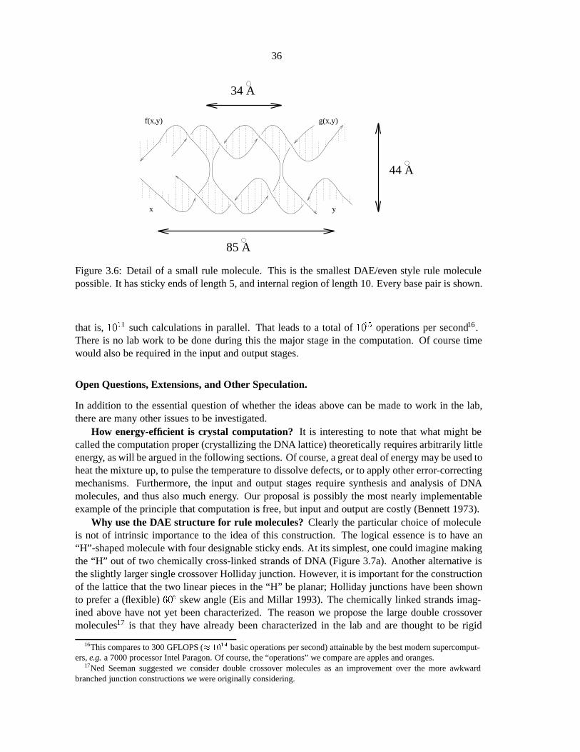
36
85 A
34 A
44 A
g(x,y)f(x,y)
x y
Figure 3.6: Detail of a small rule molecule. This is the smallest DAE/even style rule moleculepossible. It has sticky ends of length 5, and internal region of length 10. Every base pair is shown.
that is, 1011 such calculations in parallel. That leads to a total of 1015 operations per second16.There is no lab work to be done during this the major stage in the computation. Of course timewould also be required in the input and output stages.
Open Questions, Extensions, and Other Speculation.
In addition to the essential question of whether the ideas above can be made to work in the lab,there are many other issues to be investigated.
How energy-efficient is crystal computation? It is interesting to note that what might becalled the computation proper (crystallizing the DNA lattice) theoretically requires arbitrarily littleenergy, as will be argued in the following sections. Of course, a great deal of energy may be used toheat the mixture up, to pulse the temperature to dissolve defects, or to apply other error-correctingmechanisms. Furthermore, the input and output stages require synthesis and analysis of DNAmolecules, and thus also much energy. Our proposal is possibly the most nearly implementableexample of the principle that computation is free, but input and output are costly (Bennett 1973).
Why use the DAE structure for rule molecules? Clearly the particular choice of moleculeis not of intrinsic importance to the idea of this construction. The logical essence is to have an“H”-shaped molecule with four designable sticky ends. At its simplest, one could imagine makingthe “H” out of two chemically cross-linked strands of DNA (Figure 3.7a). Another alternative isthe slightly larger single crossover Holliday junction. However, it is important for the constructionof the lattice that the two linear pieces in the “H” be planar; Holliday junctions have been shownto prefer a (flexible) 60� skew angle (Eis and Millar 1993). The chemically linked strands imag-ined above have not yet been characterized. The reason we propose the large double crossovermolecules17 is that they have already been characterized in the lab and are thought to be rigid
16This compares to 300 GFLOPS (� 1014 basic operations per second) attainable by the best modern supercomput-
ers, e.g.a 7000 processor Intel Paragon. Of course, the “operations” we compare are apples and oranges.17Ned Seeman suggested we consider double crossover molecules as an improvement over the more awkward
branched junction constructions we were originally considering.
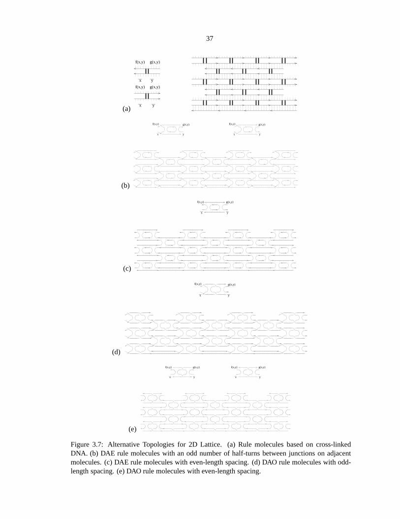
37
(a)x
f(x,y) g(x,y)
y
f(x,y) g(x,y)
x y
(b)
x y
f(x,y) g(x,y) f(x,y) g(x,y)
x y
(c)
x y
f(x,y) g(x,y)
(d)
x y
f(x,y) g(x,y)
(e)
x y
g(x,y)f(x,y)
x y
g(x,y)f(x,y)
Figure 3.7: Alternative Topologies for 2D Lattice. (a) Rule molecules based on cross-linkedDNA. (b) DAE rule molecules with an odd number of half-turns between junctions on adjacentmolecules. (c) DAE rule molecules with even-length spacing. (d) DAO rule molecules with odd-length spacing. (e) DAO rule molecules with even-length spacing.

38
(which may help prevent tangled lattices) and planar (Fu and Seeman 1993). We chose DAE inpreference to other topological variants of double crossover molecules, such as DAO, because thetopology of the rule molecule leads to a different “weave” of DNA strands in the lattice (Fig-ure 3.7bcde). We prefer to have a single strand which, if covalently linked, runs along an entirelevel of the lattice, thus encoding the BCA state for that time step.
Why a 1D BCA? Why not build a 3D lattice to simulate a 2D BCA? We started with 1DBCA because they can be immediately explored used existing DNA technology. Two dimensionsoffers several advantages, however, such easier design of efficient computations. Perhaps moreimportantly, in higher dimensions it becomes easier to design error-tolerant rules (Gacs and Reif1988); intuitively, point defects in 2D can be filled-in from adjacent correctly-computed cells,while in 1D a point defect severs communication between the left and right side. Open question:Can the DNA rule molecules be modified so as to build 3D DNA lattices?Speculatively, onecould propose a variant of the double crossover Holliday junction, the “multiple strand doublecrossover junction” (Figure 3.8), as a means to implement the read-4, write-4 operation requiredby 2D blocked cellular automata (see e.g Toffoli and Margolus (1987), Ch. 12). Unfortunately,the proposed building-block molecule has not yet been synthesized.
AB
C
D
f3(A,B,C,D)
f4(A,B,C,D)
f2(A,B,C,D)
f1(A,B,C,D)
Figure 3.8: A possible 3D lattice of DNA for simulating 2D BCA. Four DNA double helices maybe bound together by crossover junctions (left). Sticky ends determine 2D BCA rules as the rulemolecules assemble in an alternative cubic lattice (right).
Potential uses in nanotechnology. Here we have suggested an approach to molecular compu-tation via programmable self-assembly. Programmable self-assembly may have other applications.Open question: Can cellular automata generated lattices be used to define ultra-high resolutionelectronic circuits?One possibility, along the lines investigated by Robinson and Seeman (1987),would be to conjugate nano-wire onto individual rule molecules, such that when the rule moleculesfit together, an electrical circuit is formed. This proposal differs from Robinson and Seeman’s sug-gestion in that whereas they envisioned a periodic lattice of identical memory cells, we suggestthat cellular automata rules could be used to build more complicated circuits, either in 2D or 3D.
Why use DNA at all? The principle of computing via crystallization is not restricted to DNA.Open question18: Can non-DNA-based molecules could be used to design desired computationscarried out on the surface of a growing crystal?
18Suggested by Stuart Kauffman, private communication.

39
3.1.4 Comparison with Other Approaches
Perhaps the most practical suggestion for universal computation via DNA is that of Boneh et al.(1996a). Their approach makes straightforward use of well understood laboratory techniques formanipulating DNA. They are able to simulate nondeterministic boolean circuits, which seems veryefficient for some calculations, and which gives them universal computational ability. Becausecircuits allow non-local interactions of variable, circuits can be very compact. However, it shouldbe pointed out that the computation requires a lab technician to sequence operations on multipletest tubes; the logic of the program being computed is external to the DNA, which is used as amemory. Small scale computations could be immediately attempted with reasonable chance forsuccess; however due to the weakness of single-stranded DNA and other factors, it is not clearhow this approach will scale.
Other authors have proposed DNA implementations of Turing Machines directly (e.g.Beaver(1996), Smith (1996), Rothemund (1996)). The approaches vary from using PCR to relying onrestriction enzymes. These approaches show promise, although the reliability and efficiency of thesteps is unclear. Furthermore, single-tape, single-head Turing Machines are particularly cumber-some logically; circuits will typically compute the same function in many fewer steps (and singlesteps take comparable time in both systems – on the order of hours!). In short, although they areof theoretical interest, it is unlikely that anyone will actually go into the lab and solve problemsthis way.
Our hypothetical cellular automaton implementation differs in a number of ways: First andforemost, our proposal is a “one-pot” reaction. Dump in the rule molecules encoding your prob-lem, and all the logic of the computation is carried out autonomously. No lab work is involved.Furthermore, in addition to running a massive number of computations in parallel, each cellularautomaton performs its own computation in parallel – thus fully exploiting the parallelism avail-able. The major and significant drawback of our proposal is that it makes use of chemistry whichis not yet fully understood, and thus going into the lab to do a computation this way would be areal technical challenge.
The main conclusion of this paper is that annealing and ligation alonemay be sufficient for uni-versal “one-pot” DNA computation. Whether the particular scheme envisioned here can be madeto work in the lab is a matter for further research. In any case, it is clear that better experimentalcharacterization of the chemistry of annealing is required, and may open up new possibilities forDNA based computation.
3.2 Graph-Theoretic Models of DNA Self-Assembly
Abstract19 In this paper we examine the computational capabilities inherentin the hybridization of DNA molecules. First we consider theoretical mod-els, and show that the self-assembly of oligonucleotides into linear duplexDNA can only generate sets of sequences equivalent to regular languages. Ifbranched DNA is used for self-assembly of dendrimer structures, only sets ofsequences equivalent to context-free languages can be achieved. In contrast,the self-assembly of double crossover molecules into two dimensional sheets
19Results in this section also appear in Winfree et al. (in press). Thanks to Dan Abrahams-Gessel for suggesting thecontext-free grammar result.

40
or three dimensional solids is theoretically capable of universal computation.The proof relies on a very direct simulation of a universal class of cellularautomata.
A fundamental property of DNA is that, under the right conditions, Watson-Crick complemen-tary regions of single-stranded DNA will hybridize and form a double helical structure. This prop-erty, in vitro and in vivo, can lead DNA to assume a remarkable diversity of geometric forms20.Under certain simplifying conditions, the behavior of hybridization is sufficiently predictable tobe considered as a computational primitive; i.e., a function from initial oligonucleotides to finalsupramolecular structures is computed. The computational aspects of self-assembly were ex-ploited for the first time in Adleman (1994), where linear self-assembly was used as a step insolving the Hamiltonian Path Problem. When the self-assembly of tree-like structures takes place,due to the presence of branched junctions, a slightly more powerful computation results. We re-view a two dimensional generalization capable of universal computation, as suggested in Winfree(1996b), and also suggest a concrete three dimensional self-assembly process.
In order to understand the computational implications of DNA hybridization, we will firstconsider a highly abstracted mathematical model. The physical system we would like to modelcan be described as follows:
Synthesize several sequences of DNA. Mix the DNA together in solution. Heatit up and slowly cool it down, allowing complexes of DNA to form. Chemically orenzymatically ligate adjacent strands. Denature the DNA again, and ask, what single-stranded DNA sequences are now present in the solution?
A proper answer to this question is beyond our capability, and realistically detailed modelsmight not be enlightening regarding the logical essence of self-assembly. We therefore investigatevery simple models, which, nonetheless, are sufficiently realistic that translation into real worldscenarios should be direct. We will consider a number of properties which DNA self-assemblymay be postulated to obey, and we will analyze the computational capability and the limits of anyself-assembly process which obeys those properties.
Informally, the properties we consider are:
1. Constant Temperature. The number of base-pairs required for the stability of DNA com-plexes does not change during the course of the self-assembly. We thus don’t considerannealing, where at high temperatures only long regions will hybridize but later at lowertemperatures even short regions can hybridize, but rather we model a “constant tempera-ture” process.
2. Perfect Watson-Crick Complementarity. Hybridization only occurs between sequenceswith perfect Watson-Crick complementarity. Hybridization of mismatching sequences, orthat which creates bubbles, branched junctions, triple helices, and other unusual structures,is not considered.
3. Permanent Binary Events. All self-assembly interactions occur between two complexesat a time, and no more. These interactions are exclusively hybridizations, joining two com-plexes together. Furthermore, in the model once two complexes join, they never dissociate.
20In vivo, not only is there single-stranded and double-stranded DNA, but branched junctions are formed duringrecombination, and trypanosomes maintain complex networks of circular DNA within which RNA editing occurs.

41
4. No Intramolecular Events. A DNA complex which has self-assembled will not interactwith itself, for example by cyclizing. Note, however, that some physically intramolecularinteractions can be modeled as a part of a binary event, as discussed below.
5. Single vs Multiple Binding Regions per Event. We will consider two cases: either (a)each binary hybridization event creates a single contiguous Watson-Crick region, else (b) thebinary events may result in the formation of several physically separated hybridized regionsbetween the two complexes. The latter case is meant to model physical situations where anintermolecular hybridization is immediately followed by an intramolecular hybridization.The case we are interested in is discussed in Section 3.2.5 (see Figure 3.15).
6. Specified Classes of Initial Complexes. Because of our constant-temperature assumption,it becomes useful to assume that some complexes have already formed prior to the stage ofself-assembly which we will consider. Later in the paper, we will consider initial complexeswhich consist of (a) oligonucleotides, (b) duplex DNA with sticky ends, (c) hairpins withsticky ends, (d) three-armed junctions with sticky ends, (e) double crossover molecules withhairpins and sticky ends, and (f) arbitrary complexes.
Properties (1), (2) and (3) are used primarily for logical simplicity. If Property (4) werechanged to allow intramolecular events, it is possible that some of our results would be slightlymodified. We will analyze how our results change under different choices for Properties (5) and(6). In Section 3.2.5, we impose an additional property in order to incorporate geometrical con-siderations for lattice self-assembly.
3.2.1 Language Theory and Grammars
Before we present our model of DNA self-assembly, we should comment on what it means tocompute by self-assembly. As mentioned above, the typical case is that one starts with a smallvariety of synthesized oligonucleotides, and one ends with great variety of self-assembled strands.The resulting strands are not random; they have certain properties that derive from being formedfrom the original oligonucleotides according to certain rules of hybridization.
An analogous situation arises in formal language theory, which has been well understood formany years. There, rather than test tubes of strands, one is interested in sets of symbolic strings,and in methods of generating them. We will sketch the basics here; for a full development seeGinsburg (1966).
An alphabetis a finite set of symbols, for example fA;C;G; Tg or f0; 1g or fx; y; z; (; );+; �g.A string over an alphabet is a finite sequence of symbols from the given alphabet, for exampleTATAA or 101011 or (x + y) � z. A languageis a well-defined, possibly infinite set of strings,for example f all strings overfC; Tg of length70g or f all prime numbers, written in binaryg orf all well-formed formulas overfx; y; z; (; );+;�gg.
Although one cannot write down each and every string in an infinite language, one can askthe membership question: is string x in language L? Note that if the language L contains allbit strings x for which function f(x) = 1, the the membership question is equivalent to booleanfunction evaluation. The membership question may be harder or easier to answer, depending on xand L. Formal language theory goes to great pains to classify languages according to how fancythe computer must be to answer the membership problem. We sketch the fundamental result dueto Noam Chomsky, known as the language hierarchy. This requires formalizing the specificationof languages by generative rules.

42
A rewriting rule x ! y, where x and y are strings, specifies that a string s = axb canbe rewritten to produce the new string s0 = ayb. A grammarG is a collection of rewritingrules together with a division of the alphabet into two groups: terminal symbolsand nonterminalsymbols, where only nonterminals appear on the left hand side of rewriting rules. Each grammaruniquely defines a language LG as follows: the string of terminals s is in LG iff it can be obtainedfrom the special nonterminal S by the repeated application of rewriting rules in some order (calleda derivation).
Grammars may be classified by what kinds of rules they use. We give examples of the threemain classes below:
Regular grammars use rules of the form A ! pB and A ! p where A and B are nonterminalsymbols and p is a string of terminals. Languages generated by regular grammars are calledregular languages. For example, consider the regular grammar GE = fS ! 0S; S !1T; S ! 0; T ! 0T; T ! 1S; T ! 1g where 0 and 1 are terminals. This grammargives rise to all bit strings with an even number of 1’s. 101011 2 LGE
because S !1T ! 10T ! 101S ! 1010S ! 10101T ! 101011. Note that during the derivationwe always have a single nonterminal at the right, where all the action takes place. Despitetheir apparent simplicity, regular languages have found extensive use in pure and appliedcomputer science, perhaps because their membership question can always be answered byan exceedingly simple abstract computer known as a finite state machine.
Context-free grammars use rules of the form A ! P where again A is a nonterminal symbol,but now P is an arbitrary string of terminals and nonterminals. Languages generated bycontext-free grammars are called context-free languages. Consider the grammar GF =
fS ! S + S; S ! M;M ! M � M;M ! (S);M ! x;M ! y;M ! zg wherethe terminals are fx; y; z; (; );+; �g. This grammar gives rise to well-formed formulas.(x + y) � z 2 LGF
because S ! M ! M �M ! M � z ! (S) � z ! (S + S) � z !(S+M)�z ! (S+y)�z ! (M+y)�z ! (x+y)�z. Note that whereas it is impossibleto generate regular languages whose strings all have long-range structure, one can generatelong-range “nested” structure in a context-free language – for example, every parenthesismust be matched in the formulas above. Context-free languages include regular languages.The membership question for context-free languages can be answered by a slightly morecomplex machine known as a nondeterministic pushdown automaton.
Unrestricted grammars use rules of the form A ! P where now A may be an arbitrary stringsof nonterminals, and P is an arbitrary string of terminals and nonterminals. Languages gen-erated by unrestricted grammars are called recursively enumerablelanguages because theyinclude every language which can be generated (enumerated) by any computational pro-cess (recursion). Recursively enumerable languages include context-free languages, regularlanguages, and much more. They are as fancy as you can get. A very simple example:consider the alphabet fS;L;R; B ;!B ; W ;!W ; 0; 1g and the grammar GP = fS ! 1; S !LR;L ! L
!
B ; L ! 1; R !
BR;R ! 1;!
B
B !
W
!
W ;!
B
B ! 0;!
B
W !
B
!
B ;!
B
W !1;!
W
B !
B
!
B ;!
W
B ! 1;!
W
W !
W
!
W ;!
W
W ! 0g where the terminals are 0 and 1.This gives rise to the rows of Pascal’s triangle mod 2. The third row 101 2 LGP
because
S ! LR ! L!
B R ! L!
B
B R ! 1!
B
B R ! 10R ! 101. Later, we will make use of asubclass of unrestricted grammars equivalent to blocked cellular automata, which generalizethe example and which are still capable of generating all recursively enumerable languages;that is, they are universal. A surprising consequence of universality is that the membership

43
question for recursively enumerable languages is sometimes impossible to answer!
3.2.2 DNA Complexes and Self-Assembly Rules
Grammars turn out to have a close relationship to the self-assembly models we discuss here.However, to make this relationship precise, we define our model formally.
A DNA complex21 is a connected directed graph with vertices labeled from fA;C;G; Tg,edges labeled from fbackbone; basepairg, with at most one incoming and one outgoing edge ofeach type at each node (thus at most four incident edges total), and where for every base pair edgex! y there is a reciprocal basepair edge y ! x. Furthermore, all base-pairing in a DNA complexmust be Watson-Crick, that is, every basepair edge must be within a subgraph isomorphic to oneof the 10 given in Figure 3.9a.
(a) T
A
T
A
T
A C
G T
A G
C T
A T
A T
AC
G
C
G
C
G
C G
CG T
AG
C
G C
GC T
AT
A (b) i j
(c) G
C
A
T
C
A
T
T
G
A
A
G
G
T
G C
A
T C
A
G
T
A
T
A
G
G
C
C
G C A
GC
T C
T A
A
T
A
A
T
T
A
T
G
C
C
G
G
G A
A G C
GC G
TG
G AT
T TC
G CT C
A
G G A A C
GT T
GGA
A T C A T
CACT
GT
A
TC
C
A G A C
CTT
C T
TG G G
TAG
GG T
A
C
G
C
A
T
C
A
T
T
G
A
A
T
TT
T
Figure 3.9: Some DNA complexes. Solid lines represent backbone edges; each dotted line rep-resents a pair of reciprocal basepair edges. (a) The 10 Watson-Crick subgraphs. (b) The validligation site. (c) A strand, a duplex with sticky ends, a hairpin with a sticky end, a 3-armedbranched junction, and a DAO double crossover (DX) unit with sticky ends.
A DNA complex (just complexfor short) represents several DNA polynucleotides bound to-gether by Watson-Crick hybridization. Note that this representation supports a rich variety ofDNA structures, but structures such as triple helices are missing; similarly, it is lacking notionsof geometry and topological linking. Also, we must be careful because it is possibly to specifyphysically impossibly structures.
It will be useful to introduce a few examples of DNA complexes, shown in Figure 3.9c. Astrandconsists of a chain of backbone-connected nodes, with no basepair edges. Strands may beeither linear or circular. A duplexconsists of two strands with contiguous basepair edges betweenthem. A duplex may optionally have a sticky-endon either end. An n-armed (branched) junctionconsists of n duplex arms arranged around a central point. A double crossover unit(DX unit)consists of two adjacent duplexes with two points of strand exchange22. For formal reasons, theempty graph � is a DNA complex.
We now define some operations on complexes. In our model, hybridization is indicated byC1 +B C2 = C3, where +
Bdenotes the formation of basepair edges B between nodes of C1 and
21Similar to the clusterin Beaver (1995).22Real DX molecules (Fu and Seeman 1993) come in a number of geometric varieties (we use “DAO” here), each
of which put constraints on the symmetry and the number of nucleotides between crossover points. We ignore theseconstraints in the theoretical section.

44
nodes of C2. If the graph consisting of both C1 and C2 and the edges B is a DNA complex,then C3 is that graph; else C3 = � (for example, if a new edge joins two T ’s). The hybridizationoperation will be used to describe self-assembly, below.
To analyze the complexes present after self-assembly, we introduce two other operations basedon ligation and denaturing. C0 = ligate(C) is obtained by adding a backbone edge from node jto node i in every occurrence of the subgraph shown in Figure 3.9b, so long as nodes i and j haveno other incident backbone edges.
To model the denaturing of a complex, we define fCig = denature(C) to be the set ofall strandsin C , i.e., each Ci is a backbone-connected component of C (with no basepair edges).Note that if C contains topologically linked circular strands, then denaturewill “magically” unlinkthem from each other23.
In analogy to formal language theory, we define a language of DNA complexesto be a well-defined, possibly infinite set of DNA complexes. We can generate a language of complexes LR;Aby applying self-assembly rulesR to an initial language A, usually finite24. The rules R specifywhich hybridizations C1+BC2 = C3 are allowed. Let LR;A be the transitive closure of A under allallowed hybridizations. In other words, (a) A �LR;A, (b) if C1; C2 2 LR;A and C1 +B C2 = C3
is allowed, then C3 2 LR;A, and (c) no other complexes are in LR;A. Now let LR;A � LR;Aconsist of those complexes for which no further hybridization is allowed; these are called terminalcomplexes. Loosely, LR;A is meant to model the DNA structures which would form given aninfinite volume of DNA and infinite time, presuming that only the hybridizations allowed by R
are physically relevant, and ignoring transient structures.We will be especially interested in the self-assembly rules25 RT
1 which allow C1 +B C2 =
C3 6= � iff (1) the subgraph of C3 induced by B contains exactly two T -mer (or longer) strandsand (2) at most two edges lead to or exit from this subgraph. Thus, RT1 allows only hybridizationof sufficiently long sticky-ends, as illustrated in Figure 3.10.
B
Figure 3.10: A hybridization C1 +B C2 = C3 allowed by R31. The edges of B are emphasized in
C3, and the subgraph induced by B has a dotted box around it.
Both ligate and denature can be generalized to set operations by applying the operation toeach complex in the original set, and taking the union of all complexes that result. Since single-stranded DNA can be identified with its sequence, written 5’ ! 3’, we can consider denature
23Circular strands are not necessary in our constructions, but they must be considered in Theorem 2(2).24Logicians may think of A as “axioms” while R may be thought of as “inference rules”.25The subscript “1” is used because these rules give rise to essentially one-dimensional complexes.

45
to be a function from sets of complexes to sets of strings over fA;C;G; T; �g, where � is used toindicate a circular DNA strand.
Finally, we note that to represent strings in alphabets � other than fA;C;G; Tg, we mayuse a prefix-free codebookC which assigns to each symbol � in � a string C� over fA;C;G; Tgsuch that no string is a prefix of another string. A DNA sequence s = s1s2 : : : sn can thenbe translated into a string C(s) over � by scanning through s from left to right: if si begins asubsequence of s which exactly matches some C� , then si is replaced by �, else si is erased; thensi+1 is processed, and so forth. For example, if � = f0; 1g, C0 = CAG, and C1 = CTC , thenC(AAACTCTCAGTCAG) = 1100.
In summary, given a finite set of complexes A, self-assembly rules R, and codebook C, we canobtain a language of complexes LR;A as well as a language of strings
LR;A;C = C(denature(ligate(LR;A))):
We now turn to our results. The theorems are stated, explained, and examples are given. Fullproofs will appear elsewhere.
3.2.3 Linear Self-Assembly is Equivalent to Regular Languages
In this section we address the question of what can be computed by the self-assembly DNA whichobeys Properties (1-4), (5a), and (6a) or (6b). This is the familiar case of the self-assembly of longduplex DNA from many small oligonucleotides or sticky-ended fragments. That is, self-assemblybegins with oligonucleotides or duplex DNA with sticky ends, and proceeds at a constant temper-ature, allowing only permanent binary events with a single perfectly complementary hybridizationsite and no intramolecular hybridization. We make this question precise in our model by asking,what languages of strings L can be achieved as L
RT
1;A;C
for some choice of T , C, and A where Acontains only linear duplex complexes?
The following26 can be proved by construction:Theorem 1. (1) For all regular languages L, there exists a positive integer T , a codebook C,
and a set of linear duplexes A such that L = LRT
1;A;C
. (2) For all positive integers T , codebooksC, and sets of linear duplexes A, L
RT
1;A;C
is a regular language.We will sketch the construction used in the proof of (1) – see Figure 3.11 for an example.
Consider a regular grammar G for L. We design sufficiently dissimilar sequences Si (we call theirWatson-Crick complements S0
i) for all the terminal and nonterminal symbols in G. For each rule
A! p1 : : : pnB, we design a duplex with a sticky end S0A
, and internal duplex region Sp1 : : : Spn ,and a sticky end SB if B is present. We also design a duplex with one blunt end and a stickyend SS , to represent the start symbol S. These duplexes make up the initial set of complexes A.T is chosen to be the length of the nonterminal sequences Si. After self-assembly, the terminalcomplexes in L
RT
1 ;Awill correspond to derivations in G. After ligation, each complex will be a
blunt-ended duplex whose sequence consists of terminal sequences interspersed with nonterminalsequences. A codebook with Ci = Si for each terminal symbol i will “erase” the nonterminalsequences; thus L
RT
1 ;A;Cwill be exactly L. 2
A sketch of the proof of (2) is as follows: we construct a regular grammar G which generatesexactly the strands in denature(ligate(L
RT
1 ;A)). This requires creating a nonterminal symbol for
each sticky end of a duplex in A, and considering all (finitely many) T -or-more base overlapsof these sticky-ends; a grammar rule is provided for each such interaction. Care must be taken
26We note that this theorem still holds when “duplexes” is replaced by “strands”.

46
A A A C
G T T
S 1T
T C
A G A
A A A C A G
G T C
S 0
S 0S
A A A C A G
G T C T T T
A A C
G T T
T C
A G
A A C
G
A A C A G
G T C T T
T 1
T 1S
T 0T
T
T
T
A
T
T C
GA
C C C
G T T TG G
S
C
G T T TG G
C C A A A C
G T T
T C
A G A
A A A C
G T T
T C
A G A
A A C
G
T T C
GA
1 1 10
A A C
G T T T
A A C
G T T
T A A A C A G
G T C T T T
GA
T C A
T
0 1
T C
A G
Figure 3.11: The initial complexes A corresponding to the regular grammar GE , and an exam-ple derivation. Note that the self-assembly of the derivation could have occurred in any order.Subsequent ligation and denaturing will produce two strands (top and bottom) from this terminalcomplex. The codebook C defines C0 = CAG and C1 = CTC . We use R3
1.
for gaps and for sticky ends which have no interactions – both lead to termination of the strandsequence, and may require a rule using the start symbol S. Translation by the codebook can beeffected by applying a nondeterministic finite state transducer (Ginsburg 1966) to LG, yielding aregular language equal to L
RT
1;A;C
. 2Thus, our model for linear self-assembly does not permit very interesting computations. It
should be emphasized that simple extensions might allow for more complex computations. Forexample, suppose hairpins appear in A in addition to duplexes. Then, for example, we could
replace the duplex for S (Figure 3.11) by the hairpinT
T
T
T
C
GT
A
T T T
C C
G G , and change the codes for 0 and 1 tothe Watson-Crick palindromes CCGG and CGCG. Now both the top and bottom strands codethe 0 and 1 sequences; furthermore, after ligation the top and bottom strands are joined togetherby the hairpin. Consequently, we generate the set of all palindromes in which the number of onesis a multiple of four – which is not a regular language! How far can we push this idea?
3.2.4 Dendrimer Self-Assembly is Equivalent to Context-Free Languages
Dan Abrahams-Gessel pointed out to me that dendrimer self-assembly looks formally identicalto context-free grammars. This observation translates very nicely into DNA self-assembly ofbranched junctions into tree-like complexes. Therefore, in this section we address the questionof what can be computed by the self-assembly of DNA which obeys Properties (1-4), (5a), and(6b-d). That is, self-assembly begins with duplexes, hairpins, and 3-armed junctions with stickyends, and proceeds at a constant temperature, allowing only permanent binary events with a singleperfectly complementary hybridization site and no intramolecular hybridization. We note thatthis form of self-assembly has not been widely studied in the lab, and that full self-assemblywould be limited not only by material but also by geometric (steric) interference and volumetricconstraints27. Nonetheless, our abstract model allows us to ask the following precise question:
27Consider a tree which branches at every opportunity. It has 2n nodes within n steps of the center; but the volumeof space within n steps grows only as n3.

47
what languages of strings L can be achieved as LRT
1 ;A;Cfor some choice of T , C, and A where A
contains only duplexes, hairpins, and 3-armed junctions?An extra complication that immediately arises is the possibility that circular strands may form.
Recall our convention that denature returns “dotted” sequences to represent circular strands, butdidn’t specify which permutation of the circle to use. It becomes convenient to work with equiva-lence classes of sequences, where �S�= �T if the sequences S and T are circular permutations ofone another. Languages L1 and L2 are deemed equivalentif for every sequence S in one language,there is an identical or equivalent sequence T in the other language.
The following28 can be proved by construction:Theorem 2. (1) For all context-free languages L, there exists a positive integer T , a codebook
C, and a set of duplexes, hairpins, and 3-armed junctions A such that L = LRT
1 ;A;C. (2) For
all positive integers T , codebooks C, and sets of duplexes, hairpins, and 3-armed junctions A,LRT
1;A;C
is equivalent to a context-free language.
C C C
G G T TG T
A A C
C
C
G G G G G
A
G
T C C CG
A
C
C
G
G
T
T
C
T
A
T
CG
T
A
T
M y
A A A C C C C
G G G A TG T
S M
S S+S
A A C C C T
T
T
T C
T
GGGG
M x
M M*M
M z
M (S)
A A C C T
T
T
T C
T
GGG
A
T
A A C C
G TG T
A A
TT T
T
A A C C
T
T
T C
T
GGG
G
C
A A A C C C
G G G
CG
T
C
C
G
C
C
C
G
T
T
T
CT
G
G
T
T
T
GA
G
A
S
T
+ *
(
)
z
x
y
Figure 3.12: The initial complexes A corresponding to the regular grammar GF . The codebookC defines Cx = CCTT; Cy = TTCG; Cz = CATT; C( = CACA; C) = TGTG; C+ = ACCA,and C
�= TCCT . We use R3
1.
We will sketch the construction used in the proof of (1) – see Figure 3.12 and 3.13 for anexample. The construction is similar to that in Theorem 1. Consider a context-free grammarG for L. Note that there is an equivalent grammar G which uses rewriting rules of the formA ! pBqCr where p, q, and r are (possibly null) strings of terminal symbols, and A, B, and Care single nonterminal symbols (or null). Again, we design sufficiently dissimilar sequences Si forall the terminal and nonterminal symbols used inG. For rules of the formA! pB or A! Bp (Bnot null), we design a duplex as before. For rules of the form A! p, we design a hairpin with thesequences for p in the stem. We design a 3-armed junction for each rule of the form A! pBqCr
(B and C not null); it has sticky ends for S0A
, SB , and SC , and the sequences for p, q, and r are
28We note that this theorem still holds when “duplexes, hairpins, and 3-armed junctions” is replaced by simply“complexes”. That is to say, this is a fully general theorem for self-assembly under RT1 .

48
placed on the arms. As before, we design a blunt-ended duplex for the start symbol S. Thesecomplexes make up the initial set of complexes A. As before, at the appropriate “temperature” T ,the terminal complexes will correspond to derivations inG, and ligation will convert each complexinto a single strand which encodes the derivation. Processing with the codebook for the terminalsymbols will “erase” the nonterminal sequences, and L
RT
1;A;C
will be exactly L. 2
AA
AC
CC
C
GG
G
AT
G
TS M
S M
S S+S
S M
M x
M (S)
M y
M M*M
M z
A A A C C C C
G G G A TG T
A A A C C C C
G G G A TG T
C C C
G G T TG T
A
AC
CC
T
T
TT
C
T
GG
GG
A
AC
C
T
T
TT
C
T
GG
G
A
T
S
S
S
SS
S
B
AS’
p
q
r C
AA
AC
CC
GG
G
C
G
TT
T
CC
TG
CA
GG
C C C
+
T
y
A A C C
T
T
T C
T
GGG
G
CTTTGGTG
A
x
A
AC
C
G
T
G
T
A
A
T
T
T
T
)
*
A A C
G G G G
T C C C
(
TA
TG
GT
C
GA
CC
CT
CC
GA
G
AT
T
G
z
Figure 3.13: An example derivation by self-assembly of the complexes A corresponding to theregular grammar GF . Note that the self-assembly of the derivation could have occurred in anyorder, using R3
1. Subsequent ligation will produce a single strand from this terminal complex.Inset: the three-armed junction corresponding to the generic rewriting rule A! pBqCr.
The proof of (2) also follows the form of the proof of Theorem 1, only now we construct acontext-free grammar G which, loosely speaking, generates sequences corresponding to backbonepaths through complexes in ligate(L
RT
1 ;A), where gaps are filled in with the symbol 3, and where
several (but not necessarily all) permutations of each circular strand are given using �. This lan-guage is then passed through a nondeterministic transducer which returns the strand sequencesin fA;C;G; Tg and circular strand sequences in fA;C;G; T; �g. As before, the final strings areproduced by another nondeterministic transducer, which this time translates using the codebook.Thus the final language is context-free, and is equivalent to L
RT
1;A;C
. 2More intuitively, we can reason that because no intramolecular hybridizations are allowed by
RT1 , the initial complexes can aggregate only into tree-like structures. No matter how convoluted

49
the original complexes are, paths through the resulting tree-like structures are well modeled bycontext-free languages.
Our model of self-assembly of DNA into tree-like structures has strictly more computationalpower than the model of linear self-assembly. However, it is still a far cry from universal com-putation. It turns out that when we attempt to model intramolecular interactions, in the form ofcooperative binding sites, a much more powerful model results. We consider a particular case inthe following section.
3.2.5 Two Dimensional Self-assembly is Universal
To prove that two dimensional self-assembly can be universal, it suffices to demonstrate a re-stricted class which is universal. We review the class of structures introduced in Winfree (1996b),which are geometrically based on a lattice of double crossover (DX) units of DAO type Fu andSeeman (1993). It was shown in Winfree (1996b) that the self-assembly of DX units can directlymimic the operation of an arbitrary one dimensional cellular automata system. An example isshown in Figure 3.14, where a simple blocked cellular automaton rule (corresponding to the un-restricted grammar GP of Section 3.2.1, but without the termination rules) is used to generate aSierpinski triangle pattern.
The model of self-assembly used here follows Properties (1-4), (5b), and (6e), and it is moti-vated by additional physical concerns. As shown in Figure 3.14, the hybridization events may nowinvolve twobinding sites arranged as a slot. Geometry becomes important; only sticky ends whichare close to each other and arranged properly may form a slot where binding can occur. Physically,one sticky end of an unattached DX unit would hybridize to one side of the slot, followed shortlyby (the now intramolecular) hybridization of the DX unit’s other sticky end to the slot’s otherbinding site. For full computational generality, it is critical that a DX unit which matches one sitein a slot, but not the other site, will not hybridize to the lattice. Under appropriate conditions, DXunits which bind to only one site in a slot would soon dissociate, while fully matching DX unitswould bind nearly irreversibly. We therefore model slot-filling as a single permanent binary eventinvolving two binding regions, and T is chosen so that single-site binding will not occur.
We emphasize that this form of DNA self-assembly has not yet been demonstrated experimen-tally, although we report some preliminary results in Section 4.1.
We must define new self-assembly rules: RT2 allows hybridizations allowed by RT1 , and addi-tionally allows two-region slot-filling hybridizations between complexes containing the subgraphsshown in Figure 3.15, so long as the total number of basepair edges in B is at least T . This rule ismeant to model local geometry in complexes; it will be a good model only for certain structures,including (we believe) the ones used in our construction.
The following can be proved by construction:Theorem 3. (1) For all recursively enumerable languages L, there exists a positive integer
T , a codebook C, and a set of duplexes and DX units A such that L = LRT
2;A;C
. (2) For allpositive integers T , codebooks C, and sets of duplexes and DX units A, L
RT
2 ;A;Cis equivalent to a
recursively enumerable language.The proof of (1) is based on the constructions in Winfree (1996b). As cellular automata are ca-
pable of universal computation, for example by directly simulating Turing machines, we concludethat two dimensional self-assembly is universal. (2) follows because there is an algorithm for gen-erating all the complexes in LR;A so long as R is computable: keep trying new hybridizations ofcomplexes known to be in the language, and remember the resulting complex. 2
Although universal, one dimensional cellular automata are not often a convenient model forcomputing functions of interest, although they are faster and more efficient than 1-tape Turing

50
B
W
B
W W
W W W
BB
B
B
B
B
B
B
BB
W
W W
WBW B B B
B BB W
W
L L R R
S LRL L
L’
R RR’
W’ B’
B’ W’
B’ B’
W’ W’
W W
B B W
W W
R
L
Figure 3.14: An algorithmic pattern in a self-assembled lattice. At the top, the seven initial DXunits in A are shown (the black dot is a visual aid to identify “black” complexes), involving 22oligonucleotides. The corresponding rewriting rules from GP are presented in boxes. The unitsuse 12 unique sticky end sequences, denoted by fL;R; B ;!B ; W ;!Wg and their complements L0
etc. The L and R sequences are both length T ; the other sequences are length T=2. Upon self-assembly according toRT2 , a V-shaped chain of the lower three units is formed due to hybridizationof L and R, while the open slots in the initial chain are filled by the unique unit whose sticky endsmatch those on both sides of the slot. In this example, the process continues indefinitely. Eachstrand in ligate(L
RT
2 ;A) represents one or two columns of Pascal’s triangle mod 2.
B B
Figure 3.15: Two allowed slot-filling hybridizations in R62. These graphs represent requires sub-graphs of the complexes C1 and C2 in C1 +B C2 = C3. Other positions of nicks are also allowed,as are other lengths of the duplex regions.
Machines, due to their parallelism.
3.2.6 Solving the Hamiltonian Path Problem
As a concrete example of using two dimensional self-assembly for computation, we will solve thesame Hamiltonian Path Problem (HPP) used in Adleman (1994). Recall that the problem is to

51
find a path from node 1 to node N which visits every node in G exactly once. Our algorithms forsolving HPP will be based on:
1. Generate all paths from node 1 to node N .
2. In each path, sort the vertices into increasing order.
3. For each path, check that the result is exactly “1; 2; 3; : : : ; N”.
4. Output any path which passes the test, if one exists.
In a preparatory step, DNA sequences are designed for the given graph and synthesized. Steps1-3 will occur as a single self-assembly step, while Step 4 consists of sequencing circular DNA ofknown length.
For the graph used in Adleman (1994) (shown in Figure 3.16a), N = 7 and we will requirea total of 68 DX units of DAE type. Shown in Figure 3.16b, units 1 through 20 are responsiblefor Step 1 of the algorithm (the bottom layer in Figure 3.17a,b); these units are analogous to theoligos in Adleman’s solution29. Units 19 through 61 are responsible for Step 2 of the algorithm;sorting is accomplished by the Odd-Even Transposition Sort (Knuth 1973). When the symbol1has travelled all the way to the right, the sorting is complete and Step 3 is initiated, using units 62through 68.
Each terminal complex either (a) encodes a valid Hamiltonian Path, in which case the com-plex is complete (Figure 3.17a), and ligation cyclizes the outer ring, but not the inner ring30; or(b) encodes an invalid path, in which case the terminal complex contains unfilled, open slots (Fig-ure 3.17b) and will produce no cyclic strands when ligated31. Thus Step 4 can be achieved byseparating cyclic from linear DNA strands (e.g. by 2D gel electrophoresis, by exonuclease di-gestion, or by affinity purification based on the DONE sequence) followed by amplification andsequencing.
Let us briefly compare this molecular algorithm to the one used in Adleman (1994). To solvea graph with N nodes and E edges, Adleman used roughly N +E oligos and N laboratory steps.We would use roughly E2=N +N2 +N DX units (each requiring up to 5 strands) and a constantnumber of laboratory steps (synthesis, annealing, sequencing)32.
Because two dimensional self-assembly can simulate arbitrary cellular automata, similar algo-rithms can be designed for any computational purpose. For example, an N -variable size s Circuit-SAT problem can be solved using roughly Ns DX units and a constant number of laboratory stepsafter synthesis.
29Adleman’s oligos encoded individual edges in the graph, whereas ours encode pairs of edges. Also, knowing thata Hamiltonian path in this graph must visit exactly 7 nodes, our units are devised such that only odd-length paths canform completely.
30This can be ensured either by leaving an unmatched base on the sticky ends for interior units, or by phosphorylatingonly units which occur on the outer edge.
31Note that if a path visits a node twice, there will be a gap in the “Step 2” portion of the terminal complex; if a pathfails to visit some node, there will be a gap in the “Step 3” portion of the terminal complex.
32How feasible these imagined laboratory steps would be is, of course, an open question. However, once the labora-tory techniques have been debugged, conceivably our algorithm could be carried out in a single day’s work – regardlessof the size of the graph (volume permitting). A concern is that, more so than in Adleman’s algorithm, the success of ouralgorithm is critically dependent upon ligation yields. For example, if ligation is 80% effective, then only 0:830 = 0:1%of the correct terminal complexes will be fully cyclized in our N = 7 graph. Also, since each path requires a DNAmolecule roughly 100 times larger than the DNA used in Adleman’s algorithm, greater reaction volumes will be neces-sary.

52
3.2.7 Three Dimensional Self-Assembly Augments Computational Power
A trivial corollary of the universality of two-dimensional self-assembly is that if three dimensionalstructures are allowed, self-assembly is still universal. It is of greater interest if we can exploit allthree dimensions to allow for more efficient or more reliable computations. We propose a scheme
(a)
1
6
42
3
5
7
(b)
C’ C’
8
i’ ’
i-1
i
C C
1’ 7’
6
1
DONE
i { 2 ... 6 }
a { 2 ... 6, } a,b { 2 ... 6, }
c’a
b c
c’a
8 c b
7
7’
7
1
1’
1
b
b
8 8
min(a,b) max(a,b)
a’b’a’
a
a’
a
1’
1
7’
7
c
c
a b c 71 c a b c
41types
7
types
a { 2 ... 6 }
types
a b
a,b,c { 2 ... 6 } a b c a
20
Figure 3.16: (a) The 7 node graph G. (b) Rule molecules (DAE type) for solving the Hamilto-nian Path problem. Sticky ends of length T=2 are f1; 2; 3; 4; 5; 6; 7;1; C1 ; C2; C3; C4; C5; C6gand their complements; sticky ends of length T are f1 ; 2 ; 3 ; 4 ; 5 ; 6 ; 7 g and their complements.DONE is a special sequence which indicates completion of a lattice. The variables i; a; b; c areused to concisely represent a multiplicity of rule molecules; italicized variables indicate length Tsticky ends. For example, in the lower set, 15 units are designed from the central schema, one foreach pair of incident paths a! b; b! c.

53
(a)
1
1
1
1
1
1
1
1
1
1
1
1
7
7
7
7
7
7
C6
C5
C4
C3
C2
C1
DONE
15
73 6
2
88
1
8
8
8
84
4 5
4
4
5 2
2 3
3
2 5
2
2 4
3
3
3
3
3
3
3
3
4
4
4
4
4
6
78
6
6
6
6
6
6
6
5
5
5
5
5
5
2
2
2
2
2
2
2
3
4
(b)
1
1
1
1
7
7
7
7
7
7
C6
7
7
1
1
18
8
1
8
8
8
2
2
2 3 4
73 6
2
3
3
3 6
6
6
6
6
6
5
5
5 2
25
5
3
4
4 2
42
3 4
8
8
3 4 5
6
7
8
8
6
5
5
4
2 3
3
3
2
2
3 2
2 3
6
542
3
Figure 3.17: Terminal complexes after annealing. Black dots show nicks which will be ligated.(a) The lattice verifying the Hamiltonian path 1452367. (b) The lattice rejecting the invalid path123452367.
to do exactly that, again for concreteness using DAO units as our basic building block. In thissection, we will present some physical considerations, but we will not formally define RT3 .
We begin by noting that the solid angle between two adjacent DAO units is determined bythe length of the linker arm between them. For the planar lattice, we choose a length such thatthe angle is approximately 180�. Alternatively, we can choose lengths such that the angle is near120�, the appropriate value for a “honeycomb lattice” as shown in Figure 3.18.
As in the case of the two dimensional lattice of DAO units, computation is brought about byjudicious choice of the sticky end sequences on several DAO units. The three dimensional latticethus formed is equivalent to the space-time history of a 2D blocked cellular automata.
The particular incarnation of three dimensional lattice chosen here is clearly not unique, andit is suggested more as a brain-teaser than as a serious proposal; other geometries are possible,perhaps having preferable practical characteristics.

54
2 13
Bb
a A
A
Bb
B
A
a
A
B
a
b
a
b
2
3
1
(a) (b)
(c)
16 bp12 bp 11 bp
Figure 3.18: Plan for three dimensional lattice. (a) Three cross-sections through the final lattice,corresponding to the three sections indicated in (b). Circles represent cross-sections through adouble helix of DNA; bars indicate which helices are part of the same DAO unit. (b) Relativeangles of five DAO units are indicated. For perfect 120� angles, helical twist between 31.5 and35.5 �= bp is required. (c) Detail of the DAO units. A single DAO unit, with sticky end a comple-mentary to A and b complementary to B, suffices to generate the entire lattice. For computations,the sticky ends are indexed s.t. ai binds only Ai and bi binds Bi.
3.2.8 Discussion
We have analyzed the computational power of three different regimes of self-assembly in our ab-stract model, and we have speculated on an extension into the self-assembly of a three dimensionallattice.
The essential construction in the linear case is due to Adleman (1994) who used it to constructpaths through graphs. Boneh et al. (1996b) and Winfree (1996b) observed that linear self-assemblyis capable of generating regular languages. Here, we state the result in the context of our formalmodel, and we show that linear self-assembly of duplexes is limited to regular languages. Thispoint requires making the distinction between self-assembly processes with and without hairpins,as shown by the palindromes example. Linear self-assembly has been exploited in many laboratoryexperiments – both by molecular biologists and by people interested in molecular computation –and although its intricacies are not completely understood, there is a wide foundation of practicalexperience.
The self-assembly of branched junctions into dendrimer structures seems to be a relativelyunexplored idea. For example, in Ma et al. (1986) it is observed that identical three-armed junc-tions with two complementary sticky ends can cyclize. If cyclization cannot be prevented, manycontext-free grammars would be impossible to implement by self-assembly. Another concerncomes from geometry: if the desired tree-like structure contains too many branches, steric hin-

55
drance may prevent further associations from occurring. Thus it is not known to what extent thetechnique will be practical.
The self-assembly of DX units into a two-dimensional lattice is also an unconventional idea,yet to be demonstrated in the laboratory. Some first steps in this direction are reported in Sec-tion 4.1, where the slot-filling reaction is explored.
It is interesting to observe that the Chomsky Hierarchy of languages, developed originallyfor the study of human languages, also arises naturally in the study of self-assembling structures.The progression from regular to context-free to recursively enumerable languages can be seen toparallel both (a) the progression from linear to dendrimer to planar lattice structures, and (b) theprogression from “rule molecules” with effectively one input and one output, to those with oneinput and two outputs, to those with two inputs and two outputs.
One should note that all the previous arguments ignored the kinetic framework implicit in theprocess of annealing that we originally consider. Specifically, we expect that longer complemen-tary regions hybridize first. Annealing could be represented in our model as recursive computationof languages:
LannealR1;A;C= C(denature(ligate(L
R11 ;LR2
1;LR3;:::
)))
The kinetic aspects of this model of linear self-assembly may themselves be exploitable for com-putation. Intermolecular interactions other than the ones considered here might also provide com-putational advantages. Issues of concentrations and finite supply of DNA must also go into anymore practical analysis.
3.3 Simulation of Self-Assembly Thermodynamics and Kinetics
Abstract33 Winfree (1996b) proposed a Turing-universal model of DNAself-assembly. In this abstract model, DNA double-crossover molecules self-assemble to form an algorithmically-patterned two-dimensional lattice. Here,we develop a more realistic model based on the thermodynamics and kineticsof oligonucleotide hydridization. Using a computer simulation, we investigatewhat physical factors influence the error rates (i.e., when the more realisticmodel deviates from the ideal of the abstract model). We find, in agreementwith rules of thumb for crystal growth, that the lowest error rates occur at themelting temperature when crystal growth is slowest, and that error rates canbe made arbitrarily low by decreasing concentration and increasing bindingstrengths.
Early work in DNA computing (Adleman 1994; Lipton 1995; Boneh et al. 1996a; Ouyanget al. 1997) showed how computations can be accomplished by first creating a combinatorial li-brary of DNA and then, through successive application of standard molecular biology techniques,filtering the library to identify the DNA representing the answer to the mathematical question. Inthese approaches, the problem to be solved determines the sequence of laboratory operations to beperformed; the length of this sequence grows with problem size, intimidating many experimentalresearchers. Consequently, a few researchers have begun looking into chemical systems capable
33Results in this section also appear in Winfree (in press a).

56
of performing many logical steps in a single reaction, thus leading to paradigms for DNA com-puting where the problem to be solved is encoded strictly in DNA sequence; a fixed sequence oflaboratory operations is performed to determine the answer to the posed question. Promising ap-proaches include techniques based on PCR-like reactions (Hagiya et al. in press; Sakamoto et al.in press ; Hartemink and Gifford in press; Winfree in press b) and techniques based on DNA self-assembly (Winfree 1996b; Winfree et al. in press; Jonoska et al. in press). Although there has beenexperimental work exploring all these models, typically only a few logical operations have beendemonstrated. It is at this point unclear how well any of the techniques can be scaled up. Short offull experimental demonstration, realistic simulations of the chemical kinetics and thermodynam-ics can shed light on what can be expected of these systems, and can point to parameter regimeswhere the experiments are most likely to succeed. This paper presents a preliminary analysis ofthe self-assembly model of Winfree (1996b).
To motivate the self-assembly model, we consider the physical process of crystallization. Dur-ing crystal growth, monomer units are added one-by-one at well-defined sites on the surface ofthe crystal. There may be more than one type of monomer, in which case there may be severaldifferent types of binding site, each with affinity for a different monomer; typically a periodicarrangement of units results. The question of whether periodic lattices will necessarilyresult hasbeen studied in mathematics in the context of two-dimensional tilings (Grunbaum and Shephard1986). A set of geometrical shapes (the tiles) are said to tile the plane if the tiles can be arranged,non-overlapping, such that every point in the plane is covered. A surprising result in the theory oftilings is that there exist sets of tiles which admit only aperiodic tilings (Berger 1966; Robinson1971), the most elegant being the rhombs of Penrose (1978). The variety of aperiodic patterns islimitless: using square tiles with modified edges, the time-space history of any Turing Machinecan be reproduced by the tiling pattern34 (Wang 1963; Robinson 1971). Is it possible to trans-late these results back to a physical system, to produce aperiodic crystals, or even crystals which“compute”? Already, there is an extensive literature on “quasicrystals” (Steinhardt and Ostlund1987), materials which exhibit “prohibited” 5-fold symmetry and which are thought to be relatedto the aperiodic Penrose tiles. The purpose of this paper is to examine the suggestion in Winfree(1996b) that DNA double-crossover molecules can be used to make programmable “molecularWang tiles” that will self-assemble into a 2D sheet to simulate any chosen cellular automaton. Ithas already been shown experimentally that double-crossover molecules can be designed to as-semble into a periodic 2D sheet (Winfree et al. 1998) and that a single logical step can proceed ina model system. In this paper we argue that it is physically plausible to perform Turing-universalcomputation by crystallization.
3.3.1 An Abstract Model of 2D Self-Assembly
The results in the theory of tilings are entirely existential, saying nothing about howa correct tilingis to be found. What is missing is a mechanism for producing tilings. In this section we describethe relation of computation and self-assembly by presenting an abstract model of two-dimensional(2D) self-assembly, which we call the Tile Assembly Model. The fundamental units in this modelare unit square tiles (also called monomers) with labelled edges. We have an unlimited supply oftiles of each type. Aggregatesare formed by placing new tiles next to and aligned with existingones such that sufficiently many of their edges have matching labels. Tiles cannot be rotated orreflected. To define the model completely, we must be precise about when “sufficiently many”
34Even more is possible: there exist tile sets which produce non-recursivepatterns (Hanf 1974; Myers 1974)! How-ever, it is unlikely that any physical process could give rise to non-recursive patterns, in any computable amount oftime. All models discussed in this paper are strictly computable.

57
edges match. Each edge label �i has an associated strengthgi, which must be a non-negativeinteger. At “temperature” T , an aggregate of tiles can grow by addition of a monomer wheneverthe summed strength of matching edges exceeds T (mismatched labels neither contribute norinterfere) – these are called stableadditions. We say that a set of tiles P producesaggregate Afrom seedtile T if A can be obtained from the single tile T by a sequence of zero or more stableadditions of monomers; in which case, we also say simply that P produces A (if there is no needto specify the seed tile).
To illustrate this model, consider the 7 tiles shown in Figure 3.19d. The four tiles on the leftare called the rule tiles because they encode addition mod 2; the three tiles on the right are theboundary tiles; the one with two strength-2 edges is the corner tile. There are 4 edge labels, ofstrengths 0, 1, 1, and 2. At temperature T = 0, every possible monomer addition is stable, andthus random aggregates are produced. At temperature T = 1, at least one edge must match foran addition to be stable, but now the arrangement of tiles within an aggregate depends upon thesequence of additions. At temperature T = 2, there is a unique choice for the tile in each positionrelative to the corner tile, independent of the sequence of events. Under these conditions, this setof tiles produces the Sierpinski Triangle by computing Pascal’s Triangle mod 2. At temperatureT = 3, no aggregates are produced because no monomer addition to another monomer is stable.
(d)
(c)
1
1
1
1 0
2 1
2 0
2
00
2 21
11
1
2
11
1
1
1
1
1 1
1
(a)
T = 0
(b)
T = 2T = 1
Figure 3.19: The Sierpinski Tile set is shown in (d). The strengths of edges are marked, and theedge labels are denoted graphically. In (a) - (c), small tiles are used to indicate possible stableadditions to the aggregate. (a) When T = 0, any tile addition is stable, and a random aggregateresults. (b) When T = 1, typically several stable possibilities at each site; again, a randomaggregate results. (c) When T = 2, there is a unique possibility at each site, resulting in uniquepattern formation.
Whereas it is impossible to uniquely produce non-trivial aggregates when T = 0, an arbitrary

58
shape can be produced at T = 1 by assigning a unique tile to each position and giving each edgea unique label. However, this requires the use of many tiles. At T = 2 we can produce interestingpatterns with few tiles.
A hint of the computational power of the Tile Assembly Model when T = 2 is provided bya simulation of cellular automata35. The proof we develop below demonstrates two importantpoints. First, even though tile addition is stochastic, a unique pattern is produced regardless of theorder of events, because only stable tile additions are made. Second, the arrangement of tile typeson the 1D growth front of the aggregate can represent information (much like how the arrangementof 0’s and 1’s on a 1D tape represents information for a Turing Machine), and stable tile additionscan modify that information by specified rewrite rules, resulting in fully general computation.
Our simulation is based on one-dimensional blocked cellular automata (BCA)36, a variety ofcellular automaton (CA). The example of Pascal’s Triangle mod 2 (Gardner 1966) has been studiedas a cellular automaton by Wolfram (1984). It is known that BCA and CA are Turing-universalmodels, and simple simulations of Turing machines have been demonstrated (Smith 1971; Biaforepreprint). We begin by defining BCA.
Definition: A k-symbol BCA is defined (using the integers f1; 2; : : : ; kg = Zk) by a ruletable
R = f(li; ri)! (l0i; r0
i)g � (Zk �Zk ! Zk �Zk):If R is a function, then the BCA is termed deterministic. The statec of the BCA assigns a symbolto every location on an infinite linear array of cells. At each time step every cell in ct is rewrittento produce ct+1; thus we use ct(x) to denote the symbols written in cell x after t steps. The BCAuses R to re-write pairs of cells in c, alternating between even and odd alignments of the pairing:for even t and even x, and for odd t and odd x,
�(ct(x); ct(x+ 1))! (ct+1(x); ct+1(x+ 1))
�2 R:
An input to a BCA computation is a state c0 with a finite number of non-zero cells. For conve-nience and without loss of generality, we will confine our attention to n-bit binary inputs b, andwrite c0 = b to refer to an input where c0(i) = bi for 1 � i � n and c0(i) = 0 otherwise.
The computation of the BCA defines ct(x) over the half-plane t � 0. We will show how toconstruct a set of tiles P such that in all aggregates produced from the seed tile T0, if there isa tile at position (i; j) with respect to the seed tile, then the tile has edges encoding ci+j(i � j)
and ci+j(i � j + 1). Thus the time-history of the BCA computation is reproduced exactly in theself-assembled tile aggregate.
First we show, for any n-bit BCA input b, how to generate the set of n + 3 input tilesI(b).Figure 3.20a shows the construction. Because the only edge matches possible with these tiles arestrength 2, at T = 2 all produced aggregates are essentially as shown, with variable length regionsencoding “zero” on either side. The tile whose top edges encode bits b1 and b2 is referred to asthe seed tile T0 and is used as the reference for indexing tiles by location. The bottom of each
35This result, presented in less detail in Winfree (1996b), translates Wang’s simulation of Turing Machine executionby the Tiling Problem (Wang 1963) into the Tile Assembly Model given here. The Tiling Problem can be viewed asasking for the ground state of an N-state Ising model, which can be seen as a question of equilibrium thermodynamicsin the limit as T ! 0. Not only can Ising models be produced which are Turing-universal because the ground statereproduces the space-time history of any chosen Turing Machine, but the proof that tiles sets can be found which tilethe plane non-recursively shows in fact that the ground state of an Ising model can be non-recursive. Thus it is essentialto study a kinetic, rather than thermodynamic, model.
36BCA (Wolfram 1994) are also known as partitioning CA (Margolus 1984) and as 2-body CA or particle machines.They generalize the lattice gas model (Hardy et al. 1976), and are commonly studied in two dimensions.

59
input aggregate contains only strength-0 edges, so no further additions can occur there. The top ofeach input aggregate contains exclusively strength-1 edges, arranged in a zig-zag forming seriesof binding sites, called slots, where a new tile could make contact with two strength-1 edges. Foraggegates containing the seed tile T0, these edges encode the input c0 and the pairing of cells.
LL s1 s2 s2
s3 s3s4 R R
s4 RL L s1L s2s2 s3 s3 R R
s1LL LL L s2s2 s3 s3 s4 R R R R R
s1 s2LL s2
s3 s3s4 R R R RL
L R Rs1L s2
s2 s3 s3 s4 R R R
s1 s2 s2s3 s3
s4 R R
r’l r
l’
r’l r
l’ r’l r
l’r’l r
l’r’l r
l’
r’l r
l’ r’l r
l’ r’l r
l’
T0 (b)
j
i
i+j = 0
(a)
Figure 3.20: Using the Tile Assembly Model to simulating a BCA computing from a binary input.(a) Input tiles I(b) for b = 10011101, and an aggregate they produce at T = 2. Here we useconventions similiar to Figure 3.19 to indicate the strength of edges: thick edges are strength-0,doubled edges are strength-2, and all other edges are strength-1. (b) Schematic showing a ruletile generated from the BCA rule (l; r)! (l0; r0), and an aggregate produced by the rule tiles andinput tiles. Note the dotted lines indicating the default coordinate system with origin at the seedtile T0. In this schematic, the edge labels for the rule tiles are not identified.
Next, for BCA rules R we generate a set PR of k2 tiles as shown in Figure 3.20b, using onetile for each rule (l; r) ! (l0; r0). All of these rule tiles have exclusively strength-1 edges, so atT = 2 they cannot form aggregates with themselves; they must be seeded by the input tiles. Thus,when the tile sets PR and I(b) are mixed, rule tiles can sit down in the slots presented by theinput aggregates iff both of the presented edges match. Consider an aggregate in which: (1) onlyrule tiles are present above i + j = 0, and (2) every rule tile has both of its lower edges correctlymatched. It follows directly from the definitions that the edges presented by the tile at (i; j) hasedges encoding ci+j(i � j) and ci+j(i � j + 1) because this is true of the input tiles, and everyrule tile respects the update rule for the BCA. What remains to be shown is that (1) and (2) holdfor every aggregate produced at T = 2. This is done by induction on N , the number of rule tilesin an aggregate. For convenience, we refer to an aggregate containing exactly N rule tiles as anN -aggregate.
Base case: (1) and (2) hold for any 0-aggregate.Induction: Assume (1) and (2) hold for all N -aggregates. Note that (1) and (2) together imply
that above i + j = 0, the exposed edges of the aggregate are all upper edges. Any (N + 1)-aggregate must be produced from an N -aggregate by a sequence of stable additions of input tilesfollowed by a stable addition of a rule tile. (1) holds for the new aggregate because all exposededges above i + j = 0 are upper edges labelled from Zk, while all lower edges of input tiles arelabelled from fL;R; s1; : : : ; sng. (2) holds for the new aggregate because a rule tile must match

60
two edges to be added, and only upper edges are presented, so the rule tile’s two lower edges mustmatch. 2
Thus, we have proven:Theorem: Let R be a BCA, and let c(t; x) be the value of cell x at time t for a computation
on input b. If an aggregate produced from seed T0 by the tile set P = PR [ I(b) has a tile inposition (i; j), then the tile’s upper edges encode ci+j(i� j) and ci+j(i� j + 1).
In other words, the Tile Assembly Model uses asynchronous and self-timed updates to sim-ulate any deterministic one-dimensional BCA. Similar arguments can be used to show that theTile Assembly Model can simulate any non-deterministicone-dimensional BCA, in the sense thatevery possible aggregate produced according to the Tile Assembly Model will represent a possiblehistory of execution of the non-deterministic BCA. In this case, R will contain rules with identicalleft-hand sides, and consequently in some slots multiple rule tiles will match both exposed edges;thus a non-deterministic choice must be made. Alternatively, a non-deterministic set of input tilesmay be used to generate a combinatorial set of possible input strings, followed by deterministicevaluation of each input. The potential for non-determinism is important for using self-assemblyto solve combinatorial search problems in the spirit of Adleman (1994).
3.3.2 Implementation by Self-Assembly of DNA
We follow Winfree (1996b) in developing a molecular implementation of the Tile AssemblyModel: each tile is represented by a DNA double-crossover (DX) molecule (Fu and Seeman 1993)with four sticky ends whose sequences represent the edge labels. We would like these molecular“tiles” to self-assemble into a two-dimensional sheet according to the rules of the Tile AssemblyModel (see Figure 3.21). Thus, we need to show:
1. Double-crossover molecules can designed to self-assemble into two-dimensional crystal lat-tices – in preference over, for example, random tangled nets, tubes, or other structures. Thishas in fact now been demonstrated in an experimental system (Winfree et al. 1998).
2. The strengths of edge labels in the model can be implemented by designing the sticky endsequences with specific energetics of hybridization. The DNA hybridization strengths de-pend primarly on the number of base pairs, with adjustments for their particular sequence,the buffer conditions, and temperature. Thus, for example, longer sticky ends can be usedto represent edge labels with greater strength.
3. The binding of DX molecules into slots, where two sticky end sequences must both hy-bridize, is cooperative– thus, strengths “add”. We will argue below that this is a priorilikely; furthermore, suggestive experimental evidence has been presented in Winfree et al.(in press).
4. There is a physical parameter analogous to T which determines the strength required forassociation of molecular tiles. This parameter can be, for example, the temperature T . DNAsticky ends bind more strongly at low temperatures, and conversely, at higher temperaturesmore sticky-end interactions will be necessary for stable addition.
5. All these considerations can come together to produce molecular self-assembly in accor-dance with the Tile Assembly Model.

61
r’l r
l’
W(l)
C(l’) C(r’)
W(r)
(a) (b)
Figure 3.21: The DNA representation of Wang tiles. (a) A molecular Wang tile (double crossovermolecule) representing the rule (l; r) ! (l0; r0). The molecule consists of an interior structuralregion and four double-stranded arms, each terminated by a single-stranded sticky end. Edgelabels are implemented using unique sticky-end sequences. Note that sticky-ends for the loweredges use Watson-sense sequences for each label, while the upper edges use the complementaryCrick-sense sequences. This ensures the proper relative orientation of tiles. As shown, the samemolecule represents both a Wang tile and its reflection about the vertical axis; however, using fourencodings for each label (Wleft;Wright; Cleft; Cright) eliminates reflection-sense binding. In thedouble crossover molecule, the crossover points are circled, and dots are placed at the 50 endsof each strand. Color is used to indicate the edge label being represented, and not the identityof strands (each strand is multi-colored). (b) The self-assembly of 9 molecular Wang tiles, of 5distinct types. These correspond to the 9 tiles at the bottom of Figure 3.19c. Note that the cornerand boundary molecules have hairpin sequences, and thus no sticky ends, on certain of their lowerarms; this implements a tile with strength-0 labels on its lower edges. Also note that on the cornerand boundary molecules, the red and orange sticky ends are sufficiently longer than the sticky endson the rule molecules to implement a strength-2 interaction.
Our approach for arguing these points is based on the study of the thermodynamics and kineticsof DNA oligonucleotide hybridization (Wetmur 1991). We review here the elements of this theorythat are needed for our discussion.
Let ssDNA1 and ssDNA2 be two Watson-Crick complementary oligonucleotides, and let ds-DNA be the double-stranded helical complex that results upon their hybridization. The reactioncan be modelled as a two-state first-order system:
ssDNA1 + ssDNA2
kf���*)���kr
dsDNA:
We can write a differential equation for the rates of change of the concentration of each species.The units for kr are 1/sec, so kr [dsDNA] gives the rate in M/sec of dissociation of the double helix;the units for kf are 1/M/sec, so kf [ssDNA1][ssDNA2] gives the rate in M/sec of hybridization toform new double helical molecules. Altogether, we have:
� _[dsDNA] = _[ssDNA1] =_[ssDNA2] = kr [dsDNA]� kf [ssDNA1][ssDNA2]

62
The rate constants kf and kr can be estimated from the DNA sequence and the temperature T(in K), assuming the reaction is taking place in a standard buffer. For very short oligonucleotides,the forward reaction has a diffusion-controlled rate-determining step (Quartin and Wetmur 1989)approximately independent of oligo length and sequence, so:
kf = Af e�Ef=RT � 6� 105 /M/sec;
where Af = 5 � 108 /M/sec and Ef = 4 kcal/mol is the activation energy for the reaction37.The reverse rate, on the other hand, is very sensitive to oligo length and sequence:
kr = kfe�G
�s=RT ;
where R = 2 cal/mol/K and �G�s < 0 is the free energy released as heat by a single hy-bridization event38. The standard free energy �G�s can be calculated from the standard enthalpy�H�s and the standard entropy �S�s of the reaction: �G�s = �H�s � T�S�s . For reactions takingplace in commonly used buffers, the standard enthalpy and entropy can be reliably estimated fromthe sequence according to a nearest-neighbor model (SantaLucia et al. 1996); however, for thepurposes of this discussion, we can use the coarser approximation for length-s oligonucleotides39 :�H�s � �8s kcal/mol and �S�s � �22s � 6 cal/mol/K. Thus we can predict both kf and kr forthe hybridization of complementary oligonucleotides. This allows us to predict the equilibriumconcentrations of each species via the equilibrium constant
K:=
[dsDNA][ssDNA1][ssDNA2]
=kf
kr= e��G
�s=RT :
We will use our understanding of oligonucleotide hybridization kinetics and thermodynamicsto build a plausible model for the self-assembly of DX molecules via the hybridization of theirsticky ends.
3.3.3 A Kinetic Model of DNA Self-Assembly
The self-assembly of two-dimensional lattices from a heterogeneous mix of N DX molecules is afar more complicated system than the hybridization of two oligonucleotides. Rather than havingjust three species to consider (ssDNA1, ssDNA2, and dsDNA), we now have an infinite numberof species (all possible aggregates). For each aggregate of n tiles with m available sites, thereare Nm association reactions and n dissociation reactions. Note that at every available site, thereis an association reaction for every possible monomer, regardless of whether the monomer is the“correct” one or not; to understand when correct behavior can be expected, we must look closely atthe kinetics of all the reactions. The model we develop here can be seen as an extention of Erickson(1980), which considers the self-assembly of an isotropic two-dimensional lattice consisting of asingle unit type. To model the kinetics of self-assembly, we make several simplifying assumptions:
1. Monomer concentrations will be held constant. Further, all monomer types will be held at
37We will ignore the activation energy in what follows, because we will see that the value of kf has no effect on thebehavior of the system except to set the scale of the time axis.
38The more negative �G�s is, the more heat is released upon association and the more favorable the reaction is.Another way of looking at it is that if �G�s is very negative, a lot of heat must simultaneously converge upon a singledouble helical DNA molecule in order to cause dissociation, and thus dissociation is rare. Also note that here, aselsewhere, e�G
�
s=RT has an “invisible” unit of M, so that kr is in units of 1/sec.
39The empirical value �Sinit = �6 cal/mol/K can be considered the entropic cost of aligning the two strands tohave the same orientation, and is called the initiation entropy.

63
the same concentration. Primarily we make this assumption because the analysis is easier.Later we show how the results found with the assumption can be used to understand themore general case when the assumption is not true40.
2. Aggregates do not interact with each other; thus the only reactions to model are the addi-tion of a monomer to an aggregate, and the dissociation of a monomer from an aggregate.Potential drawbacks of this assumption will be discussed at the very end.
3. As in the hybridization of oligonucleotides, we assume that the forward rate constants forall monomers are identical. In particular, the forward rate constants for correct and incorrectadditions are identical.
4. As in the hybridization of oligonucleotides, we assume that the reverse rate depends ex-ponentially on the number of base-pair bonds which must be broken, and that mismatchedsticky ends make no base-pair bonds. This amounts to assuming that binding on multipleedges is cooperative and that mismatched sticky ends do not affect the dissociation rate inany way.
The model is governed by two free parameters, both of which are dimensionless free ener-gies: Gmc > 0 measures the entropic cost of fixing the location of a monomer unit (and thus isdependent upon monomer concentration), and Gse > 0 measures the free energy cost of break-ing a single sticky-end bond; both are expressed with respect to the thermal energy RT . A thirdparameter, the forward rate constant kf , is immaterial to the behavior of the system; it sets theunits for the time axis. The behavior of the system can be understood independently of the exactcorrespondence of these abstract parameters to more realistic physical parameters; however, wesketch the correspondence below.
For convenience, we lump location, orientation, and other entropic factors together into an“effective concentration” of monomers, [DX]. In these units, [DX] = [DX]=20, kf = 20kf , andthe initiation entropy of �Sinit = �6 cal/mol/K = �R ln 20 disappears from the equations. Nowwe write the concentration of each monomer as [DX] = e�Gmc . Thus the rate of associations of aparticular monomer type at a particular site on a particular aggregate is
rf = kf [DX] = kfe�Gmc ;
measured in 1/sec. To determine the dissociation rate of a unit bound by b sticky-end bonds, eachof length s, we will use our assumption of cooperativity to justify using the free energy of a singlelength-b � s oligonucleotide, �G�
b�s. To write the dissociation rate in terms of Gse, we have:
rr;b = kfe�G
�b�s=RT = kfe
�bGse ;
also measured in 1/sec. Using the values for �H�s and �S�s determined for oligonucleotide hy-bridization, sticky ends of length s would correspond to Gse = (4000K
T� 11)s. If strength-1 edge
labels are encoded with sticky ends of length s (b = 1), then strength-2 edge labels will be en-coded with sticky ends of length 2s (b = 2). If b is the sum of the strength of all a tile’s matchingedges, then the tile’s dissociation rate will be rr;b, and we will call b the number of (sticky-end)bonds.
The various reactions possible in this model, which we call the Kinetic Assembly Model, areillustrated for the Sierpinski Tiles in Figure 3.22.
40There is some intrinsic interest in the case where the assumption is true; for example, biological self-assemblyoften occurs in the context where genetic circuitry controls the concentration of the monomers via a feedback loop.

64
rf
rr,0
rf rr,2rf rr,1
rf
rr,1 rf
rr,2
rf
rr,5
Figure 3.22: The rates of reactions for various tile association and dissociation steps in the KineticAssembly Model. Note that all on-rates are identical, and that off-rates depend only upon the totalstrength of correct edge matches. Mismatched edges and empty neighbors are treated identically.
We now wish to understand the behavior of the Kinetic Assembly Model as a function of it twofree parameters, Gmc (controlled by monomer concentration) and Gse (controlled by temperatureand by sticky-end length). Our naive prediction is that the ratioGmc
Gseplays the role of T in the Tile
Assembly Model. If for small 0 < � < 1
T :=Gmc
Gse
= b� �;
then for a tile with b matches at a site,
rf
rr;b= ebGse�Gmc = e�Gse > 1;
and the site will tend to be filled. But a tile with b� 1 matches will have
rf
rr;b= e�(1��)Gse � 1;
and the tile will tend to dissociate. Because at equilibrium for the local site, the correct tileis preferred over incorrect tiles by a factor of eGse , we expect that for large Gse, the KineticAssembly Model will with high likeliness produce aggregates produced by the Tile Assembly

65
Model. To confirm this expectation and delineate when it applies, we will have to understandwhen local equilibrium is achieved, when the kinetics works in our favor, and when it worksagainst us.
We begin our detailed analysis by simulating the behavior of the Kinetic Assembly Model.Because there are an infinite number of possible aggregate types, we cannot simply integratethe rate equations to determine the time evolution of the concentration of each aggregate type.However, since aggregates do not interact with each other, we can develop our simulation fromthe perspective of an individual aggregate, starting with a chosen seed unit. Reaction rates nowbecome probability rates for a Poisson process: the association or dissociation of a monomer fromthe current aggregate. In such a simulation, the probability of observing a particular aggregate atsimulated time t corresponds to the fractional concentration of that aggregate at time t accordingto the full model.
The simulation proceeds as follows: A 2D array is used to store the arrangement of tiles inthe current aggregate. Initially the array contains all zeros to indicate empty sites, except for theorigin, which contains the seed tile. To determine the next event, the rates of all possible reactionsmust be known. All m empty sites adjacent to the aggregate are counted; the net on rate is
kon =mkfe�Gmc :
For all occupied sites (i; j) within the aggregate (except for the seed tile at the origin), the tiletypes of its neighbors are noted and the total strength bij of all matching labels is calculated; thenet off rate is koff =
Pb koff;b where
koff;b =X
ij s.t. bij=bkfe�bijGse :
Thus the net rate for events of any kind is kany = kon + koff , and the time until the next eventoccurs, �t, is chosen according to the Boltzman distribution Pr(�t) = kanye
kany�t. Now, giventhat an event has occurred, the probability that it is an on-event is kon=kany , in which case allsites and all tile types are equally likely to be chosen; otherwise a dissociation has occurred, andthe probability that some site with b bonds dissociates is koff;b=koff , and again all such sites areequally likely. Once the event is chosen and the array is updated, all rates must be recalculated todetermine the next event41.
3.3.4 Simulation Results
This section discusses simulations of the self-assembly of the Sierpinski Tiles using the KineticAssembly Model. An example run is shown in Figure 3.23. Several features of this simulation runwarrant comment.
Shape: The growth front does not advance synchronously, but rather performs a biased randomwalk, with the following restriction: because stable addition occurs only at concave cornersites (slots) on the growth front, no sites can be more than one step ahead of or behind itsneighbors. The growth front is concave on average: the boundary tiles grow fastest becausetheir growth site is always available, while internal regions on the growth front grow slowerbecause stable addition can occur at only a fraction of sites at any given time.
41The actual computer code is optimized to remove redundant calculations, of course!

66
Errors: For the most part, the Sierpinski Triangle is accurately reproduced. However, incorrecttiles do appear. In the first three frames, incorrect tiles can be seen on the border of theaggregate. These are inconsequential errors due to the equal on-rates of all tiles; they willfall off immediately and cause no permanent errors. However, in the last frame we see anincorrect tile which has been embedded within the aggregate; although it has a mismatchwith its predecessors, successive tile additions have been correct with respect to the error,and now the erroneous tile has 3 matched edges. It has caused a permanent error, and themisinformation spreads to all downstream cells in the computation.
Array Size: In the last two frames, the size of the aggregate has exceeded the size of the arrayused in the simulation. Thus the Kinetic Assembly Model is not perfectly simulated; amaximal size of aggregate is imposed. In the simulations below, this does not affect theresults in the region of interest, but it does explain the constant size (the maximum) foundduring fast, random aggregation.
Figure 3.23: Growth of the Sierpinski Triangle. Greyscale indicates the tile type in the aggregate.The simulation uses parameters Gse = 8 and T = 1:95, and the seed is a corner tile. These valuescorrespond to monomer concentration of 3 �Mand rf = 2 /sec, with sticky ends of length 5, andT = 45�C; the frames show growth after 9, 18, 36, 63, 99, and 162 seconds.
To map out the parameter space of this model, simulations of the Sierpinski tiles were per-formed for all 1 � Gmc; Gse � 30. Each simulation was run for 60=rf simulated seconds, thuson average each unoccupied site could experience up to 60 on-events of each type; consequently,the distribution of aggregate sizes is comparable across different parameter values. Figure 3.24shows the results for (a) aggregates seeded by the corner tile and (b) aggregates seeded by a ruletile, indicating both the resulting size of the aggregate and the number of errors42 in the aggregate.
42What’s actually calculated is the number of erroneous (mismatched) bonds, not the number of erroneous (incorrectwith respect to their neighbors) tiles; a single misplaced rule tile could be responsible for 4 such mismatched bonds.
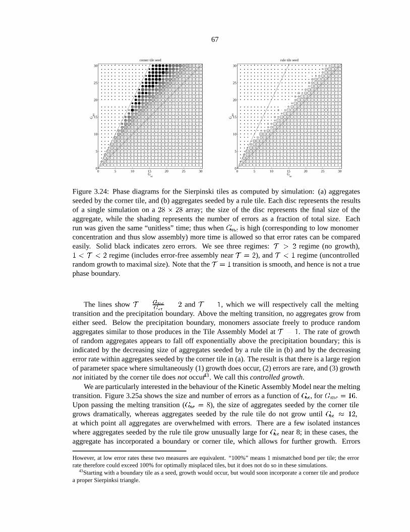
67
0 5 10 15 20 25 300
5
10
15
20
25
30
Gse
Gm
c
corner tile seed
0 5 10 15 20 25 300
5
10
15
20
25
30
Gse
Gm
c
rule tile seed
Figure 3.24: Phase diagrams for the Sierpinski tiles as computed by simulation: (a) aggregatesseeded by the corner tile, and (b) aggregates seeded by a rule tile. Each disc represents the resultsof a single simulation on a28 � 28 array; the size of the disc represents thefinal size of theaggregate, while the shading represents the number of errors as a fraction of total size. Eachrun was given the same“unitless” time; thus whenGmc is high (corresponding to low monomerconcentration and thus slow assembly) more time is allowed so that error rates can be comparedeasily. Solid black indicates zero errors. We see three regimes:T > 2 regime (no growth),1 < T < 2 regime (includes error-free assembly nearT = 2), andT < 1 regime (uncontrolledrandom growth to maximal size). Note that theT = 1 transition is smooth, and hence is not a truephase boundary.
The lines showT = Gmc
Gse= 2 and T = 1, which we will respectively call the melting
transition and the precipitation boundary. Above the melting transition, no aggregates grow fromeither seed. Below the precipitation boundary, monomers associate freely to produce randomaggregates similar to those produces in the Tile Assembly Model atT = 1. The rate of growthof random aggregates appears to fall off exponentially above the precipitation boundary; this isindicated by the decreasing size of aggregates seeded by a rule tile in (b) and by the decreasingerror rate within aggregates seeded by the corner tile in (a). The result is that there is a large regionof parameter space where simultaneously (1) growth does occur, (2) errors are rare, and (3) growthnot initiated by the corner tile doesnot occur43. We call thiscontrolled growth.
We are particularly interested in the behaviour of the Kinetic Assembly Model near the meltingtransition. Figure 3.25a shows the size and number of errors as a function ofGse, for Gmc = 16.Upon passing the melting transition (Gse = 8), the size of aggregates seeded by the corner tilegrows dramatically, whereas aggregates seeded by the rule tile do not grow untilGse � 12,at which point all aggregates are overwhelmed with errors. There are a few isolated instanceswhere aggregates seeded by the rule tile grow unusually large forGse near 8; in these cases, theaggregate has incorporated a boundary or corner tile, which allows for further growth. Errors
However, at low error rates these two measures are equivalent.“100%” means 1 mismatched bond per tile; the errorrate therefore could exceed 100% for optimally misplaced tiles, but it does not do so in these simulations.
43Starting with a boundary tile as a seed, growth would occur, but would soon incorporate a corner tile and producea proper Sierpinksi triangle.

68
7 8 9 10 11 12 13 14 15 160
100
200
300
400
500
600
700
800
Gse
size
Gmc
= 16
corner seedrule seed
7 8 9 10 11 12 13 14 15 16
10−3
10−2
10−1
100
Gse
erro
r fr
actio
n
Gmc
= 16
corner seedrule seed
0 2 4 6 8 10 12 14 16
10−3
10−2
10−1
100
Gse
Gmc
= 1.9 Gse
erro
r fr
actio
n
corner seed
Figure 3.25: (a) Simulation results for Gmc = 16 for aggregates seeded with the corner tile and arule tile. Note that for large Gse, where random aggregation is occurring, the aggregate grows tofill the entire 28 � 28 array. (b) Errors, as a fraction of aggregate size, along the line Gmc = 16.(c) Errors along the line T = 1:9, using a 38 � 38 array. Because log axes are used, data pointswhere the aggregate had zero errors are not shown.
appear to decrease exponentially as Gse ! 8 (Figure 3.25b). Figure 3.25c shows the behavioralong T = 1:9, where the system is sufficiently far below the melting transition to grow quickly,and yet sufficiently close to the melting transition to get low error rates; again, errors appear to fallexponentially with Gse.
In conclusion, it appears that with probability of error exponentially low in Gse, the kineticmodel at T = 2� � reproduces44 the Tile Assembly Model at T = 2.
44To account for the possibility that the Tile Assembly Model produces many distinct aggregates, we note that theprobability that a size-n aggregate produced by the Kinetic Assembly Model is not also produced by the Tile AssemblyModel is exponentially low.

69
3.3.5 Analysis
Equilibrium error rates. We would like to understand why the Kinetic Assembly Model pro-duces these results. We begin by analyzing the equilibrium concentrations for the reaction equa-tions. Consider an aggregate A = T �A0 where the tile T has b bonds with A0. At equilibrium, theprinciple of detailed balance tells us that45
[A]
[A0][T ]=kf
krthus
[A]
[A0]=kf [T ]
kr=
rf
rr;b= e�(Gmc�bGse):
Calculating equilibrium concentrations from any order of tile addition steps yields the same result,so we can calculate the concentration of A = T1T2 � � � Tn from any sequence of additions forproducing A. Let bi be the number of bonds for the addition
TiTi+1 � � � Tn ���*)��� Ti + Ti+1 � � � Tn;
and let bA =P
n�1i=1 bi be the total strength of all matching edges in the aggregate. Then,
[A]
[T ]=
[T1 � � � Tn][Tn]
=[T1 � � � Tn][T2 � � � Tn]
[T2 � � � Tn][T3 � � � Tn]
� � � [Tn�1 � � � Tn][Tn]
= e�(Gmc�b1Gse)e�(Gmc�b2Gse) � � � e�(Gmc�bn�1Gse)
= e�((n�1)Gmc�bAGse) = e�((n�1)T �bA)Gse :
So we see that the concentrations of aggregates with bA
n�1> T will grow with n, while the
concentrations of other aggregates will shrink46. We would like to make a prediction for errorrates based on the equilibrium assumption. To do this, we ignore the total concentration, and justask, “Of all material containing size n aggregates, what fraction is without errors?”
To compute this, we must know the value of bA for aggregates of interest. Note that for theSierpinski Tiles, any aggregate A0 produced by the Tile Assembly Model at T = 2 (i.e., anaggregate with 0 errors) has exactly bA0
= 2(n � 1) because every tile addition step contributesexactly 2 bonds. Furthermore, all other aggregates must have m :
= 2(n� 1)� bA > 0, a measureof their suboptimality47. Aggregates with small m look like perfect Sierpinski aggregates, butwith a few internal errors. For size n aggregates, one perfect and one suboptimal by m,
[Am]
[A0]=e�((n�1)T �bAm )Gse
e�((n�1)T �bA0 )Gse
= e�mGse :
This at least partly explains the absence of aggregates seeded by rule tiles: any aggregate consist-ing entirely of rule tiles must have m � 2
pn � 2, and thus their equilibrium concentrations are
45Note that rf is constant because all monomer concentrations are equal and held constant, while rr;b depends on b
for the particular reaction.46Recall that we are assuming equilibrium has been reached; taken literally, this is patently absurd when at equilib-
rium the concentrations of aggregates grows exponentially with their size. The implication is that in order to hold themonomer concentrations constant, we must continually be providing new material into the system; this new materialflows through the system to create larger and larger aggregates.
47This can be seen by noting that bA � 2#(rule tiles+corner tiles)+2:5#(boundary tiles) where the deficit isdue to internal mismatches and to the “surface energy” of unmatched edges on the perimeter. An aggregate consistingexclusively of n rule tiles will have perimeter at least 4
pn, and thus bA � 2n�2
pn and m � 2
pn�2. An aggregate
with g+1 boundary and corner tiles will have 2 mismatched or unmatched edges terminating the boundary line and onthe perimeter at least g umatched edges; thus m � 0.

70
exceedingly low48.To compute the fraction of all size-n material which is errorless, we must know how many
aggregates of each kind there are. Let nm be the number of distinct size n aggregates of sub-optimality m. Then a size n aggregate chosen from the equilibrium distribution is errorless withprobability
Preq(errorless aggregatejn) = n0[A0]P1
m=0 nm[Am]=
1P1
m=0nm
n0e�mGse
:
For small m, we can estimate nm
n0by noting that for each perfect aggregate of size n, we can make
� �2nm
�suboptimal aggregates by inducing errors at m internal edges, and completing the rest of
the pattern properly. Thus,
Preq(errorless aggregatejn) �1P
1
m=0
�2nm
�e�mGse
=1
(1 + e�Gse)2n� 1� 2ne�Gse :
We can see that Preq(errorless aggregate) � 1e
at n = 12eGse . Since the Gse is determined
by the length of sticky ends, we see that by increasing sticky end length, we can exponentiallyincrease the size over which errorless computation can be expected to occur.
We could have arrived at the same conclusion more simply, but less rigorously, by assumingthat all tile additions occur in slots and the tile is chosen independently from the local equilibriumdistribution. (A site is in local equilibriumwhen the tiles (or their absence) at neighboring posi-tions do not change, and all tile addition and tile dissociation reactions involving the site are inequilibrium.) Then,
Preq(errorless aggregatejn) � Preq(errorless step)n �
�1
1 + 2e�Gse
�n� 1� 2ne�Gse :
Note that this analysis, based on assumptions of equilibrium, predicts that error rates are unaf-fected by Gmc. This was not the result of our simulation: error rates increase dramatically as Gmc
drops below the melting transition (i.e., as monomer concentration increases). Consequently, weconclude that equilibrium is not achieved in these cases.
The kinetic trap. What prevents the system from achieving equilibrium? The intuition is thatif the growth of the crystal is faster than the time required to locally establish equilibrium at thegrowth sites, tiles will become embedded and “ frozen” in the interior of the aggregate with anout-of-equilibrium distribution.
How long does it take for a growth site to reach local equilibrium? Consider a growth site thathas just formed, and assume that the local context (neighboring tiles) does not change. Monomertiles of all kinds will sit down at the site, stay a while, and then leave, each according to its ownoff-rate. If we look immediately after the growth site appears, the probability that the site is emptyis near 100%; however, if we wait a very long time before looking, we will find each tile, or anempty site, with their equilibrium probabilities. If the local context doeschange by addition oftiles surrounding the growth site, then the tile currently in place can be “ frozen” there effectivelypermanently; even if it has one mismatched edge, three matches on its other edges can make itsoff-rate very low. Although this is a very cartoonish picture, it is the basis for our analysis, sincethe full system is too complex to treat rigorously.
48The concentration of a rule tile aggregate Ar is bounded by [Ar]=[T ] � e(T+�n�2pn)Gse , which has a minimumof [Ar]=[T ] � e(T �1=�)Gse at ncritical = ��2. (Recall that T = 2� �.) The concentration at the critical size, which

71
rr,1
rr,0
rf rr,2
r*
r*
r*
E Af
I FI
4rf
2r
C FC
0 2 4 6 8
x 10−4
0
0.1
0.2
0.3
0.4
0.5
0.6
0.7
0.8
0.9
1
seconds
prob
abili
ty
Approach to equilibrium (Gse
=3, Gmc
=5)
Empty siteCorrect tileIncorrect tiles
Figure 3.26: Model for kinetic trapping at a single growth site. (a) Simplified model for the fillingof a new site. In state E the site is empty; in state C a correct tile is present; in state A an almostcorrect tile (with one mismatch) is present; and in state I a tile with several mismatches is present.The sinks FC and FI represent frozen correct tiles and frozen incorrect tiles, respectively. (b)The approach to equilibrium distribution at the site, assuming the site has not yet been frozen. Thevertical bar marks the expected time at which the site will be frozen.
Let’s look at the probability of a particular tile being present in the site as a function of time,prior to the site being frozen. For the Sierpinski Tiles, four cases must be distinguished: (E) Thesite is empty. The “off-rate” of emptiness is 7rf = 7kf e
�Gmc , since there are 7 tiles. (C) Thecorrect tile is in place. It’s off-rate is rr;2 = kfe
�2Gse . (A) One of two tiles with just one match,and off-rate rr;1 = kfe
�Gse . (I) One of 4 tiles with no matches, and off-rate rr;0 = kf . Let pi(t)be the probability that (i) is the case t seconds after the growth site has appeared, assuming thesite has not yet been frozen. The rate equations for the model in Figure 3.26a, excluding the sinksFC and FI , can be written as
_p(t) =
26664�7rf rr;2 rr;1 rr;0rf �rr;2 0 0
2rf 0 �rr;1 0
4rf 0 0 �rr;0
37775
26664pE(t)
pC(t)
pA(t)
pI(t)
37775:=Mp(t)
and thus, p(t) = eMtp(0) where p(0) = [1 0 0 0]T .
The behavior of p(t) is shown in Figure 3.26b. We want to know the probability that thecorrect tile is in place when the site is frozen. During controlled growth, the rate of growthis approximately r� = rf � rr;2; thus a given site will be frozen in mean time approximatelyt� = 1=(rf � rr;2). With a decrease in Gmc (increased monomer concentration), rf increases, andt� becomes earlier, leading to a more out-of-equilibrium frozen distribution.
By including sink states FC and FI into the model of Figure 3.26a, we can solve exactly for
becomes a kinetic barrier to the formation of larger aggregates (Erickson 1980), approaches zero as T ! 2.

72
the frozen distribution. In this case the equations are
_p(t) =
266666664
�7rf rr;2 rr;1 rr;0 0 0
rf �rr;2 � r� 0 0 0 0
2rf 0 �rr;1 � r� 0 0 0
4rf 0 0 �rr;0 � r� 0 0
0 r� 0 0 0 0
0 0 r� r� 0 0
377777775
266666664
pE(t)
pC(t)
pA(t)
pI(t)
pFC(t)
pFI(t)
377777775:=Mp(t)
where p(0) = [1 0 0 0 0 0]T . The probability of the site being frozen with the correct tile,pFC(1), can be easily computed from the steady-state of the related flow problem, where a unitamount of material is pumped into state E and accumulates differentially in FC and FI:
_p(1) = [1 0 0 0 pFC(1) pFI(1)]T =Mp(1):
A little algebra gives the probability of an errorless step in terms of Gse and Gmc:
Prkin(errorless step):= pFC(1) =
1r�+rr;2
1r�+rr;2 +
2r�+rr;1 +
4r�+rr;0
:
In this equation for errors due to kinetic trapping, in contrast to the equilibrium prediction, theerror rate depends upon bothGse and Gmc. The equation predicts error rates that are in qualitativeagreement with the simulations, as shown in Figure 3.27. In this analysis, it becomes clear that inthe limit as T ! 2 and thus r� ! 0,
Prkin(errorless step)! Preq(errorless step) =1=rr;2
1=rr;2 + 2=rr;1 + 4=rr;0� 1
1 + 2e�Gse
:
Thus equilibrium error rates are achieved near T = 2.
0
10
20
30
0
10
20
30−6
−5
−4
−3
−2
−1
0
1
Gse
log error rate, simulated
Gmc
0
10
20
30
0
10
20
30−6
−5
−4
−3
−2
−1
0
1
Gse
log error rate, theoretical
Gmc
Figure 3.27: (a) Log10 per-step error rates, estimated from simulations. (b) Log10 per-step errorrates, according to the kinetic trap theory.

73
Speed of assembly. We have already observed that the forward rate rf = kfe�Gmc depends
upon monomer concentration, and consequently, as our error rates improve with increased Gmc,simultaneously the speed of computation drops dramatically. Now that we have an analyticalexpression for Prkin(errorless step), based upon our simplified kinetic trap model, we can de-termine the conditions which achieve a given target error rate " with the fastest rate of assemblyr� = rf � rr;2 :
1� " = Prkin(errorless step) �1
1 + 2r�+rr;2r�+rr;1
and thus for small " and 2Gse > Gmc > Gse,
" � 2r� + rr;2
r� + rr;1� 2e�(Gmc�Gse) :
= 2e��G:
To achieve error rate ", the system can be run anywhere along a line parallel to T = 1 but displacedby �G = ln2=" above it. Where along this line does self-assembly proceed most rapidly? Wefind the maximum of
r� = kf (e�Gmc � e�2Gse) = kf (e
��G�Gse � e�2Gse)
by differentiation with respect to dGse; optimal growth for constant �G occurs at
Gse = �G+ ln2 = ln4
"and Gmc = 2�G+ ln2 = ln
8
"2:
The optimal growth rate r� = kf
16"2 � 0:75� 106 "2 =sec occurs on the line Gmc = 2Gse � ln 2.
Thus it appears that we have a hard physical limit on what error rates can be achieved by DNAself-assembly within reasonable time limits. If we wish to have a net forward rate of 1 tile addedper second, then the best we can achieve is an error rate of 1/1000; while if we were willing towait half an hour for each addition, we could get an error rate of 3 � 10�5, and we could growsome perfect 200� 200 aggregates over the course of a week.
3.3.6 Discussion
The above simulations and theoretical arguments both confirm that in the Kinetic AssemblyModel, aggregates can grow with finite speed and arbitrarily low per-site error rates for largeGse and T = 2 � �. We should be careful that the analysis does not depend upon the particulari-ties of the Sierpinski Tiles. It can easily be verified that if the rule tiles use k labels (instead of the2 labels used in the Sierpinski Tiles) and there are a total of N tiles (instead of the 7 SierpinskiTiles) then the analysis is unchanged except that
Preq(errorless aggregatejn) � 1� 2(k � 1)ne�Gse
and
Prkin(errorless step) =
1r�+rr;2
1r�+rr;2 +
2(k�1)r�+rr;1 +
N�1�2(k�1)r�+rr;0
� 1� 2(k � 1)e�(Gmc�Gse)
and the optimal growth rate now occurs displaced �G =ln 2(k�1)
"above T = 1. We now loosely
discuss other aspects of the model.

74
T = 1
constant εgrowthoptimal
T = 2free
monomer
aggregationrandom
Gse
Gmc
∆ G
Figure 3.28: Analysis of the phase diagram for 2D self-assembly. Lines mark the melting transi-tion T = 2, the precipitation boundary T = 1, a line of constant error rate Gmc = Gse + �G,and the line on which optimal growth rates occur Gmc = 2Gse � ln 2.
Energy use. Reversible computers have the potential to compute using arbitrarily little energyper step, because no information is erased during the computation itself (Landauer 1961; Bennett1973). The system described here uses only fully physically reversible reactions, and thus isa candidate for low-energy computation; although non-reversible 1D cellular automata may besimulated, the 2D pattern records a history of the entire computation, and thus no information islost at any step. During controlled growth at T = 2� �, the amount of energy used by the systemequals the free energy lost as heat on each step:
��G� = �(Gmc � 2Gse)RT = �GseRT:
For any fixed Gse, error rates and energy use are simultaneously minimized as the melting transi-tion is approached.
An entropic ratchet. What happens at T = 2 exactly? We already know that at T = 2, opti-mal equilibrium error rates are achieved and no energy is used to power each step; the probabilityof going backwards is identical to the probability of going forwards. In a 1D reversible compu-tation, like that imagined by Bennett (1973), the random walk would lead to no net computationperformed. However, in our 2D system, the number of possible errorless size n aggregates growswith n. Thus, as the state-space is explored at equilibrium, it will be entropically driven to performcomputation! This oddity deserves further attention to see whether it would still be present in a

75
more realistic model.Experimentally accessibly regimes. We have already developed the relation between our
abstract parameters Gmc and Gse and relevant parameters of a real system, such as monomerconcentration and free-energies of hybridization; Figure 3.23 showed that low error rates can beachieved for realistic parameters49, given our assumptions. We can make our arguments morerealistic by considering what happens as a solution of monomers is slowly annealed from a hightemperature to a lower temperature. At any moment in time, we plot the current reaction conditionsas a point on Figure 3.24 to determine the rate of growth and per-step error rate. Suppose initiallyGmc = 12 and Gse = 5; here, above the melting transition, the monomers are all free in solution.As the temperature decreases, Gse will increase, and our point follows a horizontal trajectorystraight toward T = 2. Just below the melting transition, the aggregate will grow (with optimalerror rates for the current Gse). Consequently, the monomer concentration will drop, and Gmc willincrease, bringing the system back toward T = 2. So long as the temperature drops slowly enough,the system will stay just below the melting transition, and our point will follow a trajectory parallelto T = 2. Thus, by annealling, the self-assembly process will automatically maintain itself in theregime where errors are most infrequent. Optimal annealing schedules are an issue for futureinvestigation, and to be of practical use they will have to take account of the non-idealities of thesystem.
Imperfections of a real system. The careful reader will immediately observe that the concen-trations of different tiles will be depleted at different rates, thus breaking our original assumptionthat all tiles are present at equal concentrations. This will introduce additional factors into the erroranalysis. There are many other ways in which real systems will deviate from the Kinetic Assem-bly Model. Free energies of hybridization for different sticky-end sequences cannot be perfectlymatched, so the melting transitions for different tiles will differ slightly. Worse yet, imperfectly orpartially matched sticky-ends may contribute to the free energey of interaction between tiles withmismatched edges, in violation of the model’s assumption that only correctly edges contribute to�G�
b�s. It remains to be determined how important these factors are.
Cooperativity of binding. The Kinetic Assembly Model makes a strong assumption that twobinding sites on the same tile will act cooperatively when binding to an aggregate. Specifically, it isclaimed that �G�2 bonds = 2�G�1 bond. There are three points to make. First, the rigidity of doublecrossover molecules, as demonstrated by Li et al. (1996), suggests that the binding events shouldact together – in particular, the slot-filling event during proper growth should be cooperative. Thisintuition can be bolstered by estimating the “effective” local concentration of the remaining stickyend after one end has bound – giving an estimate for the additional “ loop entropy” (Cantor andSchimmel 1980, p. 1205) required to close the second end in the slot. Since double-strandedDNA has a persistence length of approximately 130 nt (Cantor and Schimmel 1980, p. 1033) andDX molecules span roughly 40 nt from end to end, the physical distance between the sticky endsmay fluctuate from 12 to 14 nm, thus exploring a volume of � 4000 nm3, with the free stickyend assuming perhaps a range of 30� � 30� orientations at each position. This corresponds to aneffective concentration of
Ceff =1 sticky end
4000 nm3 � 900 deg2(1024 nm3 � 3602 deg2) /liter6� 1023 sticky ends/mol
= 60mM
and thus a loop entropy �Sloop = R lnCeff = �5:6 cal/mol/K. This value is comparable with theinitiation entropy of �Sinit = �6 cal/mol/K. At 27�C it increases the free energy of interaction by
49Gmc = 30 is an example of an unrealistic parameter: at 2 pM, rf = 2 � 10�5 /sec and monomer addition will
occur only twice per day.
76
1:68 kcal/mol, which roughly offsets the contribution of a single base-pair bond (�1:4 kcal/mol).The deviation from perfect cooperativity should be negligible, according to this estimation. Exper-imental studies should be able to measure the extent of cooperativity; the preliminary experimentreported in Winfree et al. (in press) argues qualitatively for cooperativity in an analogous DNAsystem.
Second, it is possible that in addition to free energy due to sticky end hybridization and due toloop entropy, there could be enthalpic contributions to loop closure, for example, if the double he-lix must be twisted, stretched, or otherwise deformed in order to fit into the slot. Double crossovermolecule tiles can be designed with the intention of minimizing these anticooperative effects, but itremains to be seen how well that works. It may also be possible to exploitanticooperative effectsto enforce negative interactionsfor mismatching edge labels. This would require using differ-ently sized double crossover molecules, for example by changing the lengths of the four arms, sothat geometric mismatches are present in addition to sticky-end sequence mismatches. It may bepossible this way to implement a tile assembly model with negative weights.
Third, just as the initiation entropy was folded into the abstract Gmc and Gse parameters, aloop entropy or mild anticooperative adjustment could be taken up by adjusting Gmc and Gse toreproduce the on-rates and off-rates for the most important double-match and single-match cases.The simple model would be inaccurate for the off-rates of tiles with more than 2 bonds, but asthese tiles seldom dissociate for parameters of interest, this inaccuracy is irrelevant.
Alternative reaction mechanisms. The Kinetic Assembly Model assumes that the growthof aggregates occurs by addition of single monomers only, and thus that there are no interactionsbetween aggregates. Reaction mechanisms would not affect the equilibrium error rate predictions,but Rothemund (personal communication) has emphasized that dimer-dimer pathways, or other in-teractions between aggregates, could be very important for the kinetics of self-assembly, and thustheir inclusion could affect kinetic trapping in theory and in practice. Indeed, Malkin et al. (1995)have directly observed, by AFM, crystal growth by sedimentation of small three-dimensional nu-clei.
It is also possible – perhaps I should say probably – that alternative reaction mechanisms arepresent for creating non-planar structures, such as tubes or random three dimensional networks.Indeed, experimental studies attempting to create 2D lattices of DX molecules (Winfree et al.1998) found, for example, occasional unexpected rod-like structures in addition to the expectedplanar 2D crystals.
3.3.7 Conclusions
We have used a pair of simple kinetic models to understand error rates in the self-assembly processfor algorithmically-defined 2D polymerization. Our results lend credence, in lieu of a full exper-imental demonstration, to proposals (Winfree 1996b; Winfree et al. in press) for computation byself-assembly of DNA: we have found that 2D self-assembly can theoretically support computa-tion with arbitrarily low error rates. This answers a question raised by Reif (in press), who wasconcerned that, as in the T = 1 example of Figure 3.19, an unfortunate sequence of tile additionscould lead to blockageswhere no tile can fit into an empty site without a mismatch. We find thatblockages are not a problem in our model, but the thermodynamics of DNA hybridization give riseto an intrinsic per-step error rate. Large computations require low concentrations and hence veryslow growth rates. This is the algorithmic equivalent of the fact, in conventional crystallization,that large perfect crystals form under conditions of slow growth near the solubility line (Kam et al.1980).

77
A few worked-out examples for the case of the Sierpinski Tiles are illustrative. From ourinvestigations of kinetic trapping, we found that there is an optimal growth rate r� for every targeterror rate ". At this growth rate " = 4e�Gse , [DX] = 2:5"2 M, and r� = 0:75 � 106"2 /sec, where0 < Gse = (4000K
T� 11)s � ��G�=RT for the hybridization of a single sticky end of length
s. Assemblies of nmax
:= 1=" tiles would be expected to contain one error on average; there is an
inverse relationship between the rate of assembly and the expected size of error-free aggregates.For example, sticky ends of length 5 at room temperature give Gse = 12 and nmax = 40000,but requires a concentration of [DX] = 1:5 nM and thus a rate r� = 1:6 /hour. The same systemcould be run at 17�C, where Gse = 14, [DX] = 30 pM, nmax = 300000, and r� = 0:71 /day;or at 45�C, where Gse = 8, [DX] = 4:5�M, nmax = 750, and r� = 1:35 /sec. Under the latterconditions, a non-deterministic set of DNA tiles in a reasonable volume (1ml) could give rise to1013 distinct 300-tile aggregates in under a minute, that is, 1014 operations per second. This wouldbe sufficient for solving a simple 40-variable SAT problem by subsequent ligation and PCR to findthe answer-containing strand in the “good” aggregate. However, for this application an additionalsource of errors would be false-positives due to non-answer aggregates which, because of an errorduring assembly or during PCR, appear to be “good;” an additional error analysis is required inthis case.
What are we to do if we want faster and less error-prone computation? Reif (in press) suggestsusing a combination of autonomous self-assembly and step-wise processing; his ingenious con-structions perform a computation in a series of self-assembly steps each of which only requires theformation of small aggregates. Because the number of steps is kept low (for example, computinga circuit of size s requires O(log s) self-assembly steps), there is promise for asymptotically bettererror rates; however, a detailed analysis remains to be done, and may be difficult due to the lack ofexperimental evidence for the complex DNA structures and self-assembly reactions he proposes.
Is it possible to get faster and less error-prone computation in an autonomous self-assemblysystem? Biology makes use of an energy source to improve error rates by “proofreading” mecha-nisms (Kornberg and Baker 1991). Kinetic proofreading mechanisms can be fairly simple (Hop-field 1974); it would be interesting if such a mechanism could be devised to mediate the self-assembly of double-crossover molecules. Alternatively, one can accept the intrinsic error rate andtry to devise error-correcting algorithmswhich could improve the overall error rate exponentiallywith a slowdown only linear in the number of extra tile types.
78
Chapter 4 Experiments with DNA Self-Assembly
4.1 A Competition Experiment: Slot-Filling
Abstract1 In this section we examine the question of whether the two bind-ing domains in the input region of a rule molecule act cooperatively during aslot-filling reaction. A well-defined DNA system has been designed to modela single slot analogous to the one in a growing lattice. The system consistsof three logical pieces: ABC, D, and D’ . D and D’ model rule molecules whichmatch either both or just one of the slot’s two sticky ends. Thus, by competingD again D’ , we can determine the extent of the preference for D over D’ for fill-ing the slot. By analyzing ligation products, wherein a closed circular speciesindicates the correct insertion of D in the slot, we observed that D was pre-ferred even in the presence of a 64-fold excess of D’ . This is strong suggestiveevidence that the slot-filling reaction in lattice formation is also cooperative,as is required for our model of computation by self-assembly.
The theoretical studies of previous chapters only point to the possibility of algorithmically-patterned lattices of DNA. There are two major issues to be investigated experimentally. The firstis whether homogeneous lattices will form; i.e., whether the geometric structure itself will self-assemble. The second issue is whether, in the presence of multiple units in solution, the logicallycorrect unit will hybridize in each slot. This competitive process for filling each slot is essentialfor computation, as a single error can propagate throughout the entire computation. Ultimately,error rates will determine the size of lattice in which reliable computation may be performed.
We have begun an investigation of the second issue. We first build a model molecular complex,called ABC, which contains a single slot and no other sticky ends. ABC is composed of twodouble crossover molecules, A and C, and a duplex linker B. ABC is created by ligating eightoligonucleotides; the final structure contains four hybridized strands. Rather than test the assemblyof a double crossover unit into ABC’s slot, we model the unit by a linear duplex “ linker” , called D.When ABC is properly hybridized to D, we call the complex ABCD. Completely ligated, ABCD isa complex catenane with four interlocked circles. To test the specificity of the hybridization, wealso have a mismatched linker D’ , which is perfectly complementary to only one of the sticky endsin the slot. We expect that ABCD’ cannot be completely ligated, due to the mismatch, and henceABCD’ does not form a catenane. These molecular complexes are diagramed in Figure 4.1.
Experimentally, we must establish that the double crossover molecules A and C form properlyupon annealing their component strands. As developed in Fu and Seeman (1993), where the detailsof hybridization were probed by more extensive structural characterization, a good indication ofproper association is a single band of mobility in a non-denaturing gel appropriate for the topologyand molecular weight. The ligation products ABC, ABCD, and ABCD’ (by which we mean whatever
1Results in this section also appear in Winfree et al. (in press), and include joint work with Xiaoping Yang andNadrian C. Seeman, as described in Chapter 1. Thanks to John Abelson for generously providing laboratory facilitiesat Caltech for some of the experiments reported here.

79
A1 (88 nt) = TAATGTGCCTGACCGCCTTACTTTTGTAAGGCGGTCACCGAATTCCGACTTTTGTCGGAATTCGGACGCCTAACGTGGACACCGCGAC
A2 (52 nt) = GTAAGCTTCCTGTCCACGTTAGGCGTGGCACATTAGTCGCGGACTTAGACAA
A3 (32 nt) = GGATGGTTGTCTAAGTGGAAGCTTACCGCATC
B1 (64 nt) = CCATCCAGCGTTGACACGTCTGCGTAACTCACGGTAGTGTAAACCTTGATTGAATCGGCAGTAC
B2 (52 nt) = CCGATTCAATCAAGGTTTACACTACCGTGAGTTACGCAGACGTGTCAACGCT
C1 (80 nt) = TGCATCTGGACCTCGAGACTTTTGTCTCGAGGTGGTTCGCCGCTTTTGCGGCGAACCTGAACACGAACGTGGTGGATCAC
C2 (52 nt) = GAGTCGACGGACCACGTTCGTGTTCACCAGATGCAGTGATCCTGCATATGAC
C3 (32 nt) = CTGAGCGTCATATGCACCGTCGACTCGTACTG
D1 (64 nt) = GCTCAGCCGTGCTAATCCAACTCGGTACCTACAGATACGATGGACTGGTTAGATAGGTGATGCG
D2 (52 nt) = ACCTATCTAACCAGTCCATCGTATCTGTAGGTACCGAGTTGGATTAGCACGG
D1' (64 nt) = GCTCAGCCGTGCTAATCCAACTCCTGCAGTACAGATACGATGGACTGGTTAGATAGGTCAACAG
D2' (52 nt) = ACCTATCTAACCAGTCCATCGTATCTGTACTGCAGGAGTTGGATTAGCACGG
Complex ABC: A B C
TTGTCGGAATTCGG-ACGCCTAAG CACCTGT-CCTTCGAATG CAGTATACGT-CCTAGTG TGCATCTGG-ACCTCGAGACTT
TTCAGCCTTAAGCC TGCGGATTC GTGGACA GGAAGCTTAC-CGCATC CTGAGC-GTCATATGCA GGATCAC ACGTAGACC TGGAGCTCTGTT
TTGTAAGGCGGTCA GGCACATTA CAGCGCC TGAATCTGTT-GGTAGG TCGCAACTGTGCAGACGCATTGAGTGCCATCACATTTGGAACTAACTTAGCC GTCATG-CTCAGCTGCC TGGTGCA TCGTGTTCA GGTTCGCCGCTT
TTCATTCCGCCAGT-CCGTGTAAT GTCGCGG-ACTTAGACAA CCATCC-AGCGTTGACACGTCTGCGTAACTCACGGTAGTGTAAACCTTGATTGAATCGG-CAGTAC GAGTCGACGG-ACCACGT AGCACAAGT-CCAAGCGGCGTT
Complex ABCD: A D/B C
TTGTCGGAATTCGG-ACGCCTAAG CACCTGT-CCTTCGAATG GCGTAG-TGGATAGATTGGTCAGGTAGCATAGACATCCATGGCTCAACCTAATCGTGCC-GACTCG CAGTATACGT-CCTAGTG TGCATCTGG-ACCTCGAGACTT
TTCAGCCTTAAGCC TGCGGATTC GTGGACA GGAAGCTTAC-CGCATC ACCTATCTAACCAGTCCATCGTATCTGTAGGTACCGAGTTGGATTAGCACGG CTGAGC-GTCATATGCA GGATCAC ACGTAGACC TGGAGCTCTGTT
TTGTAAGGCGGTCA GGCACATTA CAGCGCC TGAATCTGTT-GGTAGG TCGCAACTGTGCAGACGCATTGAGTGCCATCACATTTGGAACTAACTTAGCC GTCATG-CTCAGCTGCC TGGTGCA TCGTGTTCA GGTTCGCCGCTT
TTCATTCCGCCAGT-CCGTGTAAT GTCGCGG-ACTTAGACAA CCATCC-AGCGTTGACACGTCTGCGTAACTCACGGTAGTGTAAACCTTGATTGAATCGG-CAGTAC GAGTCGACGG-ACCACGT AGCACAAGT-CCAAGCGGCGTT
�
�
����
���
��
-
-
��AA
AA
�
-
�
�
����
��-�
��
�
��
AA
AA
�
�
����
���
��
-
-
��AA
AA
�
-
�
�
����
��-�
��
�
��
AA
AA
-
�
614 16 10 6 52 6 6 10 16 12
B2
D1 C3
C2
C1D2A2
A1 A3 B1
84
1
Figure 4.1: Sequences and Structures for ABCD. Sequences are written 5’ to 3’ . 3’ ends aredenoted by arrows in the diagrams, and strand labels are near 5’ ends. Lengths are measured innucleotides. Above, sequence details are given along with schematic representations of ABC andABCD (not ligated). Below, more geometric detail is sketched for A, B, C, D, and ABCD (ligated).Diagrams illustrate intended structures only.
it is we get when we intend to make structures ABC, ABCD, and ABCD’ respectively) are examinedboth in non-denaturing and denaturing gels; in the former we are looking for a single band ofapproximately the correct apparent molecular weight, while in the latter we are looking for linearstrands of the lengths predicted for ligation. Ligation of double crossover molecules has previouslybeen shown to be well-behaved (Li et al. 1996). Topologically closed structures, such as ABCD,can be assayed by treating with an exonuclease (Ma et al. 1986). Although none of these testsis absolutely rigorous, together they may give us confidence that the reactions are proceeding aspredicted.
4.1.1 Materials and Methods
Sequence Design.The twelve strands required for A, B, C, D, and D’ were designed by applyingthe principles of sequence symmetry minimization (Seeman 1990), where the design process en-sures that there are no complementary regions between strands, except as desired. In short, eachdouble crossover molecule is designed by creating sequences appropriate for two asymmetric Hol-liday junctions, then juxtaposing these sequences as appropriate for a four-stranded DAO, adding

80
hairpin sequences and re-phasing A1 and C1 to put the nick in the central region of the DAO. A1’shairpin regions are longer than C1’s to allow A1 and C1 to be distinguished on gels. The lengths ofthe linkers B and D were chosen such that both DAO units should be nearly coplanar according toan estimated 10.5 base pairs per double helical full turn. Exact sequences are given in Figure 4.1.
Synthesis and Purification of DNA.All strands were synthesized on an Applied Biosystems380B automatic DNA synthesizer using routine phosphoramidite procedures (Caruthers 1985).DNA strands were purified by denaturing polyacrylamide gel electrophoresis. DNA concentra-tions were estimated by OD260. All strands were phosphorylated by T4 Polynucleotide Kinase(U.S. Biochemical or Promega), followed by phenol extraction and ethanol precipitation. DNAwas not radiolabeled, with the exception of the DNA used for Figure 4.6, for which 10% of strandswere phosphorylated with 32 -ATP and mixed with 90% non-radiolabelled strands.
Formation of Hydrogen-Bonded Complexes.Complexes A, B, C, D, and subportions thereofwere formed by mixing stoichiometric quantities of each strand at concentrations near 1 �M in 1xUSB T4 DNA Ligase buffer (U.S. Biochemical: 66 mM Tris�HCl (pH 7.6), 6.6 mM MgCl2, 10mM DTT, 66 �M ATP; or Promega: 30 mM Tris�HCl (pH 7.8), 10 mM MgCl2, 10 mM DTT, 500�M ATP). These solutions were annealed for two hours from 80�C down to room temperature.
Formation of Covalently Bonded Complexes.Complexes AB, BC, ABC, ABCD, and ABCD’were formed by mixing stoichiometric quantities of annealed A, B, C, and D’ , followed by D after20 minutes. Up to 50 units of T4 DNA Ligase (U.S. Biochemical or Promega) were added andsolutions were incubated in a 16�C water bath for 2 or 8 hours. One sample of ABCD was furthertreated by adding 1
10
thvolume 10x USB Exonuclease III buffer (U.S. Biochemical) and 100 units
Exonuclease III (U.S. Biochemical), incubated at 37�C for 1 hour. Prior to being loaded in gels,solutions for gels (a) and (b) were heated to 80�C and again annealed to room temperature, todenature proteins and re-form hydrogen-bonded complexes. For gels (c), ligation was followed byphenol extraction and ethanol precipitation, then samples were heated to 90�C for 5 minutes priorto being loaded.
Denaturing Polyacrylamide Gels.Denaturing gels contain 8.3 M urea and 8% acrylamide(19:1 acrylamide:bisacrylamide). The running buffer is TBE (89 mM Tris�HCl (pH 8.0), 89 mMboric acid, 2 mM EDTA). The sample buffer contains 0.1% bromphenol blue and xylene cyanolFF tracking dyes in 80% formamide with 10 mM EDTA. Samples are heated at 80�C for 5 minutesimmediately prior to loading. Gels are run at approximately 60 V/cm and 35 Watts, then soakedin StainsAll dye and digitized by DeskScan II on an Apple Macintosh.
Non-denaturing Polyacrylamide Gels.Non-denaturing gels contain 12.5 mM Mg++ and 8%acrylamide (19:1 acrylamide:bisacrylamide), 0.75 mm thick. The running buffer is TAE/Mg++
(40 mM Tris�HCl (pH 8.0), 20 mM acetic acid, 2 mM EDTA, 12.5 mM magnesium acetate).The loading buffer contains 0.02% bromphenol blue and xylene cyanol FF tracking dyes and 5%glycerol in ligation buffer. Gels are run at approximately 16 V/cm and 10 Watts at 4�C , thensoaked in StainsAll dye and digitized by DeskScan II on an Apple Macintosh.
4.1.2 Results
Formation of Complexes.The first question is whether the individual duplexes and double-crossover molecules A, B, C,
and D will form from their component strands. Figure 4.2 shows a non-denaturing “ formation gel”for double-crossover molecules A and C. Each lane contains a different subset of strands. Eachlane shows a single prominent band, indicating that the strands form a specific complex. Faintbands are presumably the result of poor stoichimetry. For example, a deficit of A3 in lane 5 could

81
explain the minor production of A12 in this lane. We estimate that the bands for A and C in lanes3 and 8 contain over 90% of the material; however, this is not a quantitative measurement. Themobilities of the partial complexes for A are as would be expected for double-stranded DNA of thesame molecular weight: A23 < A12 < A123. Lane 9 contains an anomolous major band: ratherthan seeing C12 at the 132nt level, we see a major and minor band above the 200 nt level. Wenow interpret this as a C12C12 dimer bound together at the self-complementary Nde I and SalI restriction sites, as shown in Figure 4.3. In the additional presence of C3, these site are doublestranded and the dimer is not produced. Only one of the arms of A has a restriction site, whichexplains why a A12A12 dimer was not also observed.
1 2 3 4 5 6 7 8 109
A12A123 A123
A23 C123C23
C123C12
MM
200 nt
400 nt
600 nt
84: A23, C23132: C12140: A12164: C172: A
264? C12C12
7% Non-denaturing PAGE
Figure 4.2: Non-denaturing gel. Lanes 1 and 10: 100 base-pair double-stranded ladder. Lane 2:A12 (140 nucleotides). Lanes 3 and 5: A123 (172 nucleotides). Two preparations of strand A1were used, which apparently have different stoichiometry. Lane 4: A23 (84 nucleotides). Lanes 6and 8: C123 (164 nucleotides). Two preparations of strand C1 were used, which apparently havedifferent stoichiometry. Lane 7: C23 (84 nucleotides). Lane 9: C12 (132 nucleotides). The bandat � 240 nt is presumably the dimer C12C12.
Figure 4.4 shows several stages in the formation of ABCD. On the non-denaturing gel, theduplexes and double crossover molecules A, B, C, and D form clean bands (a, lanes 1-4) whichmigrate with approximately the same mobility as equivalent molecular weight duplex DNA. Lig-ation products AB and BC also show clean bands (a, lanes 9-10). Ligation product ABC appears asthe major band in its lane (a, lane 8); another band appears at the level of AB and BC indicatingincomplete ligation. Ligation product ABCD also appears, we believe, as the major band in its lane(a, lanes 7 and 5); a slower unidentified band also appears. After exonuclease treatment, the major

82
CA
GA
TTGTCTCGAGGT CCAGATGCA CACTAGG GTATACGT GGATCAC ACGTAGACC TGGAGCTCTGTT TTCAGAGCTCCA GGTCTACGT GTGATCC TGCATATG CCTAGTG TGCATCTGG ACCTCGAGACTT
TTCGCCGCTTGG ACTTGTGCT ACGTGGT GTCGACGG TGGTGCA TCGTGTTCA GGTTCGCCGCTT TTGCGGCGAACC TGAACACGA TGCACCA GGCAGCTG ACCACGT AGCACAAGT CCAAGCGGCGTT
AC
AG
TTGTCTCGAGGT CACTAGG TTCAGAGCTCCA GGTCTACGT c1
TTGCGGCGAACC TGAACACGA TTCGCCGCTTGG ACGTGGT
c2
CCAGATGCA
ACTTGTGCT
GTGATCC TGCATATGAC
TGCACCA GGCAGCTGAG
TTCGCCGCTTGG ACTTGTGCT ACGTGGT
c2
c1
c2
c1
GGATCAC ACGTAGACC TGGAGCTCTGTT
TTGCGGCGAACC TGAACACGA TGCACCA GGCAGCTGAG
TGGTGCA TCGTGTTCA GGTTCGCCGCTT GAGTCGACGG ACCACGT AGCACAAGT CCAAGCGGCGTT
CAGTATACGT CCTAGTG TGCATCTGG ACCTCGAGACTT
TTCAGAGCTCCA GGTCTACGT GTGATCC TGCATATGAC TTGTCTCGAGGT CCAGATGCA CACTAGG
Nde I
Sal I
Figure 4.3: Proposed structure causing the anomolous band in Figure 4.2 lane 9. First C1 and C2hybridize to form C12, then two C12 molecules bind at self-complementary restriction enzymesites.
band of ligation product ABCD is still apparent, though diminished (a, lane 6).
On the denaturing gel, we obtain further evidence of ligation activity by observing the lengthsof newly created oligonucleotides. Lanes 1-4 can be used as markers for the lengths of most ofthe original oligonucleotides: A1 (88), A2 (52), B1 (64), B2 (52), C1 (80), C2 (52), D1 (64), D2(52). A3 and C3, both 32 nucleotides, ran off the gel. Lane 10, product AB, shows the expectedformation of A2B1 (116) and B2A3 (84); lane 9, product BC, likewise shows the formation ofB1C2 (116) and C3B2 (84); and lane 8, product ABC, shows the expected formation of A2B1C2(168) and C3B2A3 (116). Lanes 5 and 7, product ABCD, contain only three significant bands: A1(88), C1 (80), and a band which migrates slower than a 2000 nucleotide strand, according to themarker (lane 11). This slow band is exonuclease-resistant (lane 6). We therefore conclude that theband contains the catenane A2B1C2D1:A3D2C3B2; i.e., ABCD minus the A1 and C1 loops, whichapparently were not ligated. Double crossover molecules with two nicks have been shown to bestable (Zhang and Seeman 1994a), suggesting that the nicks in A1 and C1 should not significantlyaffect the formation or stability of A or C.
We wished further confirmation of the idenity of the bands. It is possible to determine exactlywhich set of oligonucleotides is present in each band by “differential labelling.” Here, we run a setof nearly identical experiments, the only difference being which oligonucleotide has been phos-phorylated with 32P. On the gel, only products incorporating the radiolabelled oligonucleotide willbe visisble. Thus, for each band, we can simply read off the lanes in which it appears to determinewhich oligonucleotides are involved in the complex. If more than one complex co-migrate, theanalysis gets more difficult. This is indeed what happens in the gels shown in Figure 4.5: on the8% gel, the outer circle and the outer:inner complex comigrate. Change in mobility with changein polyacrylamide density distinguishes different topological species, allowing us to separate theouter circle and outer:inner complex on a 5% gel. However, at this percentage, the inner circle

83
B1C2, A2B1, D1C2, A2D1A3B2C3, A3D2C3
A DCB
(exo)ABCD
ABCBC
ABM
8% Denaturing PAGE
52 nt
168 ntA2B1C2, C2D1A2,A3B2C3D2
116 nt
64 nt
A3B2, B2C3, C3D2, D2A3A1
C1
88 nt
80 nt84 nt
B1, D1
A2, B2, C2, D2
1110987654321
8% Non-denaturing PAGE
1 2 3 4 5 6 7 8 9 10 11
DCA B MBC
ABABCABCD(exo)
116 nt
172 nt
288 nt280 nt
452 nt568 nt
164 nt
ABCD
ABC
ABBC
AC
B, D
Figure 4.4: (a) Denaturing gel electrophoresis. Lane 1: A (172 nucleotides). Lane 2: B (116 nu-cleotides). Lane 3: C (164 nucleotides). Lane 4: D (116 nucleotides). Lane 5: Product ABCD withligase. ABCD contains 568 nucleotides. Lane 6: Product ABCDwith ligase and exonuclease. Lane7: product ABCD with ligase. Lane 8: Product ABC with ligase. ABC contains 452 nucleotides.Lane 9: Product BC with ligase. BC contains 280 nucleotides. Lane 10: Product AB with lig-ase. AB contains 288 nucleotides. Lane 11: 100 base-pair double-stranded ladder. Numbers atright indicate estimated positions for expected products, consistent with the marker lane. (b) Non-denaturing gel electrophoresis: Lane 1: A (172 nucleotides). Lane 2: B (116 nucleotides). Lane 3:C (164 nucleotides). Lane 4: D (116 nucleotides). Lane 5: Product ABCD with ligase. ABCD con-tains 568 nucleotides. Lane 6: Product ABCD with ligase and exonuclease. Lane 7: product ABCDwith ligase. Lane 8: Product ABC with ligase. ABC contains 452 nucleotides. Lane 9: ProductBC with ligase. BC contains 280 nucleotides. Lane 10: Product AB with ligase. AB contains 288nucleotides. Lane 11: 100 base-pair double-stranded ladder. Numbers at right indicate estimatedpositions for expected products, consistent with the marker lane.
and the 232-mer linear strand comigrate! Note that ligase was not as efficient in this experimentas it was in the previous experiment: the ABCD lane contains many partial products, indicatingincomplete ligation of nicks in the ABCD complex, or poor stoichiometry so that many ABCDcomplexes were lacking one or more strand. This is turns out to be convenient for interpretting thenext experiment, where ligation was again incomplete.
Specificity of Reaction.
Figure 4.6 shows the results of a preliminary experiment investigating the effectiveness ofD vs D’ in filling the slot created by ABC. Lane 13 contains ABC, and thus has primary bands forA2B1C2 (168) and C3B2A3 (116). Lanes 2 and 12 show ligation of ABCD in 1:1:1:1 stoichiometry.The ligation apparently was not as complete as in 4.4, as several bands of “partial products” areobserved. The fastest band is appropriate for linear A3D2C3B2 (168) and cyclical permutations;the next band is appropriate for linear B1C2D1 or D1A2B1 (180); the next major band is appropriatefor A2B1C2D1 (232) and cyclical permutations. The band below c is known from other gels(not shown) to be exonuclease-resistant, and the two cyclic molecule bands are thought to bean indicator of the formation of ABCD. Lanes 1 and 10 show ligation of ABC with respectively anequimolar amount or a 20-fold excess of D’ . We again see the linear bands of lengths 168, 180, and232, while bands at 136 (D2C3B2) and 116 (C3B2A3 and A3D2C3) become significant. Critically,the slow circular products are missing, suggesting that D’ was only ligated on the side where it

84
C1A1
D2 B3C3
D1C2A3
B1A2
ABCD
4 7 8 121 2 3 65 9 10 11
A3B2, B2C3, C3D2, D2A3A1
C1
88 nt
168 nt
A1D2 B3
C3 A3C1
C2 A2B1D1
1 2 3 4 109875 6
136 nt
136 nt
116 nt
88 nt
168 nt
232 nt180 nt
5% Denaturing PAGE8% Denaturing PAGE
80 nt84 nt
116 ntB1C2, A2B1, D1C2, A2D1A3B2C3, A3D2C3
B2C3D2, D2A3B2
A2B1C2, C2D1A2,A3B2C3D2
232 ntA2B1C2D1
180 ntB1C2D1, D1A2B1
Figure 4.5: Denaturing gel electrophoresis with radiolabelled strands. All lanes contain ABCD, butin each lane only one strand was radiolabelled. (Note that the gels were improperly dried, leadingto “smearing” after the gel was run.)
168 ntA2B1C2, C2D1A2,A3B2C3D2180 ntB1C2D1, D1A2B1232 ntA2B1C2D1
136 ntB2C3D2, D2A3B2116 ntB1C2, A2B1, D1C2, A2D1
A3B2C3, A3D2C3
8% Denaturing PAGE
64 nt52 nt
88 nt
80 nt84 nt
B1, D1
A2, B2, C2, D2
A1A3B2, B2C3, C3D2, D2A3
C1
121110987654321 13
0:1 1:1 1:4 1:16 1:641:0 1:2 1:8 1:32 0:20
0:01:0
1:1
Figure 4.6: Denaturing gel electrophoresis. All lanes contain A:B:C in 1:1:1 stoichiometry, plusvarious concentrations of D:D’ . Lane 1–9: D:D’ = 0:1, 1:0, 1:1, 1:2, 1:4, 1:8, 1:16, 1:32, 1:64.Lanes 10–13: D:D’ = 0:20, 1:1, 1:0, 0:0. (Note: the first gel was slightly ripped during staining.)
matches the slot’s sticky end. Lanes 11 and 3–9 show ligation of one unit of ABC with an x-foldexcess of D’ and equimolar D, where x ranges from 1 to 64. In every case, the closed molecule cis formed, indicating that ABCD is still formed in the presence of competing D’ . Additional bandsalso appear, possibly due to unexpected interactions involving D1 or D2.
4.1.3 Discussion
We interpret these results as follows. First, we believe that we are making the ABCD complex,with the caveat that we believe the nicks in A1 and C1 are not being sealed. This suggests that (1)in ABC, the linker B is properly spaced such that double crossover molecules A and C are roughlycoplanar, and (2) that in each double crossover molecule, the two helical axes are also roughlycoplanar. Second, we observe that D, which matches the sticky ends on both sides of ABC’s slot,

85
out-competes D’ , which matches only on one side, even when D’ is 64-fold more abundant than D.We plan to quantitate the thermodynamics of this reaction in the near future.
The experiments reported here bear on the two-dimensional self-assembly process postulatedin Section 3.2.5. These experiments are meant to model a single slot-filling step during the self-assembly of a two dimensional lattice. In our experiments, this fundamental step can occur, andwith some specificity. These results encourage us to examine this step in closer detail in the future,as well as to attempt the self-assembly of an entire sheet. We hope that the self-assembly of analgorithmically patterned sheet of DNA can eventually be verified by TEM or AFM microscopy.
The self-assembly of molecules can correspond to several well known computational classesup to and including universal computation. This suggests that external processing is not an in-trinsic element of molecular computation; computationally universal “one-pot” reactions seemplausible. We have shown some encouraging but preliminary experimental investigations into thefundamental computational step in our two dimensional self-assembly model. The generality ofthe approach used here suggests that the potential for universal computation may be widespreadamong self-assembly processes in nature. In addition to being interesting in its own right as auniversal mechanism, it may be worth considering whether the self-assembly processes describedhere could be useful technologically, perhaps as part of an approach to nanotechnology (Li et al.1996).
4.2 Experiments with 2D Lattices
Abstract2 Molecular self-assembly presents a bottom-up approach to the fab-rication of objects specified with nanometer precision. DNA molecular struc-tures and intermolecular interactions are particularly amenable to design andare sufficient for the creation of complex molecular objects. Here we reportthe design and observation of two-dimensional crystalline forms of DNA thatself-assemble from synthetic DNA double-crossover molecules. Intermolecu-lar interactions are programmed by the design of sticky ends that associateaccording to Watson-Crick complementarity, enabling us to create specificperiodic patterns on the nanometer scale. The patterned crystals have beenvisualized by atomic force microscopy.
Control of the detailed structure of matter on the finest possible scale is a major goal of chem-istry, materials science and nanotechnology. This goal may be approached in two steps, (1) theconstruction of individual molecules, represented by the triumphs of synthetic chemistry, and (2)the arrangement of molecular building blocks into larger structures. The simplest arrangement ofmolecular units, in two or three dimensions, is a crystal. Design components for crystals musthave definable intermolecular interactions and must be rigid enough to prevent the formation ofill-defined aggregates (Liu et al. 1994). Branched DNA molecules with sticky ends appear to be
2Results in this section also appear in Winfree et al. (1998), and include joint work with Furong Liu, Lisa A. Wenzler,and Nadrian C. Seeman, as described in Chapter 1. Thanks to John Abelson and his group for the use of his laboratoryand technical advice; to Anca Segall, Ely Rabani, and Bob Moision for instruction and advice on AFM imaging; and tothe Beckman Institute Molecular Materials resource center for assistance and use of their AFM facilities.

86
promising for macromolecular crystal design (Seeman 1982), because their intermolecular inter-actions can be programmed through sticky ends (Cohen et al. 1973) that associate to form B-DNA(Qiu et al. 1997); however, studies of three- and four-arm junctions reveal that the angles flankingtheir branchpoints are flexible (Ma et al. 1986; Petrillo et al. 1988).
The need for a rigid design component with predictable and controllable interactions has led tothe utilization of the antiparallel DNA double-crossover motif (Fu and Seeman 1993) for this pur-pose. Double-crossover (DX) molecules are analogs of intermediates in meiosis (Schwacha andKleckner 1995) which consist of two side-by-side double-stranded helices linked at two crossoverjunctions. Antiparallel DX molecules have been shown to possess the rigidity lacking in conven-tional branched junctions, thus suggesting that they might be suitable for use in the assembly ofperiodic matter (Li et al. 1996).
These findings stimulated a theoretical proposal to use two-dimensional (2-D) lattices of DXmolecules (Winfree 1996b) for DNA-based computation (Adleman 1994). In the mathematicaltheory of tilings (Grunbaum and Shephard 1986), rectangular tiles with programmable interac-tions, known as Wang tiles, can be designed so that their assembly must mimic the operation of achosen Turing Machine (Wang 1963). DX molecules acting as molecular Wang tiles could self-assemble to perform desired computations (Winfree 1996b; Winfree et al. in press; Reif in press).Consequently, the ability to create 2-D lattices of DX molecules assumes additional interest as astep toward the design of molecular algorithms.
Here, we report the assembly from DX molecules of three 2-D lattices with two distinct topolo-gies. The DX molecules, � 2 � 4 � 13 in size, self-assemble in solution to form single-domaincrystals as large as 2 � 8 microns with uniform thickness between 1 and 2 nm, as visualized byatomic force microscopy (Binnig et al. 1986) (AFM). By incorporating a DNA hairpin into a DXmolecule to serve as a topographic label, we have produced stripes above the surface at intervalsof 25. Two-component lattices have been assembled with a stripe every other unit.
4.2.1 Design of DNA Crystal
Our approach to two-dimensional crystal design is derived from the mathematical theory of tiling(Grunbaum and Shephard 1986; Winfree 1996b). The desired lattice is specified by a set of Wangtiles with colored edges; the Wang tiles may be placed next to each other only if their edges areidentically colored where they touch (Figure 4.7a). Our goal is to design synthetic molecular unitscorresponding to these tiles, such that they will self-assemble into a crystal that obeys the coloringconditions. As an initial demonstration of molecular Wang tiles, we have chosen the simplest non-trivial set of tiles: two tiles, A and B, which make a striped lattice (Figure 4.7a, left). Translatedinto molecular terms, we obtain DX systems that self-assemble in solution into two-dimensionalcrystals with a well-defined subunit structure.
The antiparallel DX motif (Fu and Seeman 1993) consists of two juxtaposed immobile 4-armjunctions (Seeman 1982) arranged such that at each junction the non-crossover strands are antipar-allel to each other. There are five distinct DX motifs, but only two are stable in small molecules(Fu and Seeman 1993): these are called DAO (double crossover, antiparallel, odd spacing) andDAE (double crossover, antiparallel, even spacing). The design depends critically upon the twistof the B-form DNA double helix, in which a full turn takes place in� 10:5 base pairs (Wang 1979;Rhodes and Klug 1980). DAO molecules have an odd number of half-turns (e.g. 3 half-turns is� 16 base pairs) between the crossover points, while DAE molecules have an even number ofhalf-turns (e.g. 4 half-turns is � 21 base pairs). Computer models of the DX molecules used inthis study, shown in Figure 4.7b, were generated using NAMOT2 (Carter and Tung 1996). Com-plete base stacking at the crossover points is assumed. The DAO molecules consist of 4 strands

87
36 nt, 12.6 nm
b
d
DAO-Ec
a A B
AAAA
BBBB
B AAAA
BBBB
BBBBB
BAAAA
AAAA
DAO
A
B
B^
Figure 4.7: Design of DX molecular structure and arrangement into 2-D lattices. a, The logicalstructure for 2-D lattices consisting of two units. Type A units have four colored edge regions,each of which match exactly one colored region of the adjacent type B units. Note that rotationsand reflections of Wang tiles are disallowed; an equivalent restriction could also be obtained byusing non-rectangular tiles or more complex patterns of colors. b, Model structures for DAO typeA units. Each component oligonucleotide is shown in a unique color. The crossover points arecircled. c, The lattice topologies produced by the DAO. Each DX unit is highlighted by a grey rect-angle. A unique color is chosen for each strand type which would be formed after covalent ligationof units. Arrowheads indicate the 30 ends of strands. Black ellipses indicate dyad symmetry axesperpendicular to the plane; black arrows indicate dyad axes in the plane (full arrowhead) or screwaxes (half arrowhead). d, The actual sequences used in the reported experiments (see Methods forseveral exceptions). The schematics accurately report intended primary and secondary structure– oligonucleotide sequence and paired bases – but are not geometrically or topologically faithfulbecause they don’ t show the double helical twist. Both type B and typeB are shown, indicatingwhere the hairpin sequences are inserted.
of DNA, each of which participates in both helices. The DAE molecules consist of 3 strandsthat participate in both helices (yellow, light blue, green), and 2 strands that do not cross over(red, dark blue). Each corner of each DX unit has a single-stranded sticky end with a unique se-quence; specific association of DX units is controlled by choosing sticky ends with Watson-Crickcomplementarity.
To ensure that the component strands form the desired complexes, strand sequences must bedesigned carefully so that alternative associations and conformations are unlikely. Therefore wemust solve the “negative design problem” (Seeman 1990; Yue and Dill 1992; Sun et al. 1996)for DNA: find sequences that maximize the free energy difference between the desired conforma-tion and all other possible conformations. We use the heuristic principle of sequence symmetry

88
minimization (Seeman 1982, 1990) to minimize the length and number of unintentional Watson-Crick complementary subsequences. In each DX molecule’s sequences, there are no 6-base sub-sequences complementary to other 6-base subsequences except as required by the design, andspurious 5-base complementarity is rare. Thus it is expected that during self-assembly, the DNAstrands spend little time in undesired associations and form DX units with high yield.
DX units can be designed that will fit together into a two-dimensional crystalline lattice. Herewe use two distinct DAO unit types (Figure 4.7a) to produce striped lattices. The lattices producedby this system is called DAO-E to indicate the number of half-turns between crossover pointson adjacent units; its topology is shown in Figure 4.7c. The symmetries of the DAO-E latticeis that corresponding to the layer group (Vainshtein 1994) p2122. Covalently joining adjacentnucleotides at nicks in the lattice, by chemical or enzymatic ligation, would result in a “wovenfabric” of DNA strands. Ligation of the DAO-E design produces four distinct strand types, eachof which continues infinitely in the vertical direction (in this paper, “vertical” and “horizontal”will always be as in Figure 4.7c).
Control of self-assembly to yield the 2-D lattice is obtained by two design criteria. First, thesticky-end sequences for each desired contact are unique; this ensures that the orientations andadjacency relations of the DX units comply exactly with the design in Figure 4.7a. Sticky ends arelength 5, so that each correct contact contributes approximately 8 to the free energy of associationat 25�C, according to a nearest-neighbor model (SantaLucia et al. 1996). Second, the lengthsof the DX arms and sticky ends, and thus the separations between crossover points, respect asclosely as possible the natural twist of the B-form DNA double helix; thus adjacent DX moleculesare effectively coupled by torsional springs whose equilibrium positions have been designed tokeep the adjacent DX molecules coplanar. For example, a linear rather than planar polymer couldresult if each unit makes two sticky-end bonds to each neighboring unit, but this would requireovertwisting, undertwisting, or bending of the double helix, and thus is discouraged by our design.
Figure 4.7d shows the DX units and sequences used in our experiments, except as noted inMethods. In each system, there are two fundamental DX units, called A and B, and, additionally,an alternative form B that contains two hairpin-terminated bulged 3-arm junctions (similar to theDX+J motif (Li et al. 1996)). Based on studies of bulged 3-arm junctions (Ouporov and Leontis1995), we expect that in each unit, one hairpin will point up and out of the plane of the DXcrystal, while the other hairpin will point down and into the plane, without significantly affectingthe rigidity of the molecule (Li et al. 1996). The B units will replace the B units and serve ascontrast agents for AFM imaging, because their increased height can be measured directly.
4.2.2 Materials and Methods
DNA sequences and synthesis. Figure 4.7d shows sequences used in these experiments; forhistorical reasons, some figures show experiments where variants of these sequences were used.The sequences for DAO-E A, B, and B given in Figure 4.7d were used for Figure 4.12bc. Fig-ure 4.12adef show DAO systems with symmetrical sticky ends: the sequence for the green strandsof DAO A is 50TCACT...GAGAT30 and the sequence for the blue strands of DAO B and Bare 50AGTGA...ATCTC30. All oligonucleotides were synthesized by standard methods, PAGEpurified, and quantitated by UV absorption at 260 nm in H2O.
Annealing of oligonucleotides. The strands of each DX unit were mixed stoichiometricallyand dissolved to concentrations of .2 to 2 �M in TAE/Mg++ buffer (40 mM Tris�HCl (pH 8.0),1 mM EDTA, 3 mM Na+, 12.5 mM Mg++). The solutions were annealed from 90�C to roomtemperature over the course of several hours in a Perkin-Elmer PCR machine (to prevent concen-tration by evaporation). To produce lattices, equal amounts of each DX were mixed and annealed

89
from 50�C to 20�C over the course of up to 36 hours. In some cases (Figure 4.12abc) all strandswere mixed together from the very beginning.
Gel electrophoresis studies. For gel-based studies, T4 polynucleotide kinase (Amersham)was used to phosphorylate strands with 32P; these strands were then PAGE purified and mixedwith an excess of unlabeled strands. Non-denaturing 4%, 5%, or 8% PAGE (19:1 acrylamide:bis-acrylamide) in TAE/Mg++ was performed at 4�C or at room temperature. For denaturing exper-iments, after annealing in T4 DNA ligase buffer (Amersham) (66 mM Tris�HCl(pH 7.6), 6.6 mMMgCl2, 10 mM DTT, 66 �M ATP), 1 �l = 10 units T4 DNA ligase (Amersham) was added to 10 �lDNA solution and incubated for up to 24 hours at 16�C or at room temperature. For exonucleasereactions, 50 units of exonuclease III (Amersham) and 5 units of exonuclease I (Amersham) wereadded after ligation, and incubated an additional 3.5 hours at 37�C. The solution was added to anexcess of denaturing dye buffer (0.1% xylene cyanol FF tracking dye in 90% formamide with 1mM EDTA, 10 mM NaOH) and heated to 90�C for at least 5 minutes prior to loading. Denaturinggels contained 4% acrylamide (90:1 acrylamide:bisacrylamide) and 8.3 M urea in TBE (89 mMTris�HCl (pH 8.0), 89 mM boric acid, 2 mM EDTA). Gels were analyzed by phosphorimager.
Preparation of AFM sample. 2 to 10 �l were spotted on freshly cleaved mica (Ted Pella,Inc) and left to adsorb to the surface for 2 minutes. To remove buffer salts, 5 to 10 drops ofdoubly-distilled or nanopure H2O were placed on the mica, the drop was shaken off and thesample was dried with compressed air. Imaging was performed under isopropanol in a fluid cellon a NanoScope II using the D or E scanner and commercial 200 �m cantilevers with Si3N4 tips(Digital Instruments). The feedback setpoint was adjusted frequently to minimize contact forceto approximately 1 to 5 nN. Images were processed with a first- or third-order “fl atten filter,”which independently subtracts a first- or third-order polynomial fit from each scanline to removetip artifacts; however, this technique introduces false “shadows” into the images shown here.
4.2.3 Results of Characterization by Gel Electrophoresis
A prerequisite for lattice self-assembly is the formation of the DX units from their componentstrands. A thorough investigation of this issue was done for the original studies of DX (Fu andSeeman 1993); that the new designs also behave well constitutes further validation of the antipar-allel DX motif. Because the sticky ends of A units have affinity only for sticky ends of B units,and not for themselves, neither A nor B alone in solution can assemble into a lattice. Thus theformation of isolated DX units can be monitored easily by non-denaturing gel electrophoresis, asdescribed previously (Fu and Seeman 1993), and greater than 95% of the material is seen in theexpected band for A and greater than 85% for B(Figure 4.8). Additionally, complexes are formedonly by strands which were designed to interact. However, strand 3 of B does not bind fully tostrand 4, unless strand 2 is also present. This may be due to a potential hairpin structure near the50 end of strand 3; when strand 2 binds to strand 3, we postulate that this hairpin is undone. Notealso that dimer and multimer species are not found, and in particular note that the individual A orB monomers do not assemble into extended structures, such as the desired lattice.
Solutions containing A units and B units can be mixed and annealed to form AB lattices.Lane 4 of Figure 4.9(left) shows that the self-assembled structure is too large to migrate throughthe gel, although a fraction of the material is coming out of the well in a smear. Enzymaticligation of these lattices with T4 DNA ligase produces immobile material, while the A and B
units alone are not substrates for ligation (Figure 4.9(left). The nicks in the lattice, where strandsfrom adjacent DX units abut, are all on the upper or lower surface of the lattice, where they areaccessible to the enzyme. The ligated lattice should contain long covalent DNA strands, whichserve as reporters of successful lattice formation (shorter strands report either the presence of

90
14 24 3413 12 124
1341234
234123
23
21 3 4 5 6 7 8 9 10 11 21 3 4 5 6 7 8 9 10 11
23123
2341234
134124
3412
2413
14
5% Non-denaturing PAGEA B
41
2 3
Figure 4.8: Formation gels for the A and B double-crossover molecules, run at 1�C by 5% non-denaturing PAGE. Every strand is radiolabelled so that quantitation is possible.
small aggregates or an occasional failure to ligate within the lattice). All four reporter strandsextend for more than 30 repeats when visualized by denaturing polyacrylamide gel electrophoresis(Figure 4.9, right). Longer strands co-migrate on this gel, so we cannot determine the full extentof polymerization. These results suggest that the lattice is a good substrate for T4 DNA ligase,and that the lattices can form with more than 30 � 30 units. However, unintended associations orside reactions could lead to similar distributions of strand lengths after ligation. Direct physicalobservation is necessary to confirm lattice assembly.
41
2 3
5 6 8 987654321
M MB ABABA A B
+ ligase
5% Non-denaturing PAGE 4% Denaturing PAGE
1 2 3 4 7 10 11 12
M M MB1 B2 A4B3 B4 A1 A2 A3 M
72 nt
118 nt
194 nt234 nt
1353 nt1078 nt
603 nt
281 nt310 nt
872 nt
2706 nt....
.
388 nt
236 nt
144 nt
Figure 4.9: (left) Non-denaturing gel, StainsAll stain. Lanes 2-4 show A alone, B alone, andAB together. Lanes 5-7 show A alone ligated, B alone ligated and AB together ligated. All thematerial in lane 7 is in a sharp band directly around the well (circled); this band can be seen clearlyin color, but not in the B/W rendition here. (right) Denaturing gel, with differential radiolabelling.Every lane contains either marker or ligated AB; in each lane the radiolabelled oligonucleotide isindicated below.

91
As a control to test the 4-connected nature of the putative lattice product, versions of A andB were made with certain sticky ends truncated, as shown in Figure 4.10. Av and Bv weredesigned to make vertical one-dimensional chains of DX units; Ah and Bh were designed tomake horizontal one-dimensional chains of DX units; and Ad and Bd were designed to makediagonal one-dimensional chains of DX units. However, quite unlike the AB product stuck in thewell, all three truncated systems produced what appear to be dimers on the non-denaturing gel.No ligase was used. Apparently, the chain structures are either not being made, or they are fallingapart into dimers in the gel. We do not yet understand these results.
...
1 2 3 4 5 6 7 8 9 10 1112 13
MA B A B AA BABAB AB AB
Bv v
v
h h
h
d d
d
236 nt
144 nt
388 nt
..
2706 nt
5% Non-denaturing PAGE
BA A
B
h
hh
h
A
AB
B
B
B
A
A
v
v
v
v
d
d
d
d
Figure 4.10: (left) 5% Non-denaturing gel, with radiolabelling of A3 and B3. (right) Diagram ofthe truncated DX units, and intended chain structures.
4.2.4 Results of AFM Imaging
We have used atomic force microscopy (Binnig et al. 1986) to demonstrate unequivocally theformation of 2-D lattices. A and B units are annealed separately, then combined and annealedtogether to form AB lattices. The resulting solution is deposited for adsorption on an atomi-cally flat mica surface, and then imaged under isopropanol by contact mode AFM (Hansma et al.1992). The solution is not treated with DNA ligase, and thus the lattices are held together onlyby noncovalent interactions (e.g. hydrogen bonds and base stacking). This protocol ensures thatthe solution contains no protein contaminants and demonstrates that ligase activity is not neces-sary for the self-assembly process. Negative controls of buffer alone and of A or B alone showno aggregates larger than 20 nm (Figure 4.11abc). In separate experiments, A and B DAO unitswere modified by the removal of two sticky ends from each unit (e.g. all yellow and red stickyends in Figure 4.7d); when the modified A and B units were annealed together, we observed onlylinear and branched structures with apparent widths typically less than 10 nm (Figure 4.11def),providing additional negative controls. However, the unmodified AB samples contain 2-D sheetsmany microns long, often more than 200 nm wide (Figure 4.12a). The apparent height of thesheets is 1:4 � :5 nm, suggesting a monolayer of DNA. The sheets often seem ripped and appearto have a grain, in that rips have a preferred direction consistent with the design (Figure 4.7c). Inthe DAO-E lattice, a vertical rip requires breaking six sticky-end bonds per 12 nm torn, whereasa horizontal rip requires breaking only one sticky-end bond per 13 nm torn. A possible vertical

92
column, perpendicular to the rips, is indicated in Figure 4.12a (arrows). Although in this imagethe columns are barely perceptible, Fourier analysis shows a peak at 13 � 1 nm, suggesting thatobserved columns are 1 DX wide. Periodic topographic features would not be expected in theideal AB lattice; however a vertically stretched lattice may have gaps between the DX units thatcould produce the periodic features seen here. Because crystals are found in AFM samples takenfrom both the top and the bottom of the solution, we believe that crystals form in solution and arenot due to interaction with a surface.
a b c
d fe
Figure 4.11: AFM images of buffer (a), A and B controls (b and c respectively), and sticky-end-truncation controls ABv (d), ABh (e), and ABd (f). All scale bars are 300 nm; images show500 � 500 nm, 1 � 1 �m, or 3 � 3 �m. The grayscale indicates height above the mica surface;apparent height of features is less than 5 nm.
4.2.5 Control of Surface Topography
The self-assembling AB lattice can serve as scaffolding for other molecular structures. We havedecorated B with two DNA hairpin sequences inserted into its component strands, which we callB (Figure 4.7d). So decorated, the vertical columns of the lattice become strikingly apparent asstripes in AFM images (Figure 4.12bc), further confirming the proper self-assembly of the 2-Dlattice. The spacing of the decorated columns is 25 � 2 nm for the DAO-E lattice, indicatingthat every other column is decorated, in accord with the design. Slow annealing at 20�C andgentle handling of the DAO-E sample during deposition and washing has produced single crystalsmeasuring up to 2�8 �m(Figure 4.12def). Close examination shows that the stripes are continuousacross the crystal, and thus it appears to be a single domain containing over 500,000 DX units.

93
a
d e
b c
f
Figure 4.12: AFM images of unmodified DAO-E AB lattice (a). A possible vertical column isindicated by the arrows. Fourier analysis shows 13 � 1 nm periodicity; each DAO is 12.6 nmwide. (b) and (c) show DAO-E AB lattice (two views of the same sample). Stripes have 25 � 2
nm periodicity; the expected value is 25.2 nm. (def) show a large single-domain crystal of DAO-EAB lattice at three levels of detail (all the same sample). The largest domain is roughly 2�8 �m,and contains roughly 500,000 DX units. All scale bars are 300 nm; images show 500 � 500 nm,1:5 � 1:5 �m, or 10 � 10 �m. The grayscale indicates height above the mica surface; apparentlattice height is between 1 and 2 nm.
We have also tested DAO systems incorporating only one of the two hairpins inB, DAOsystems in which the 3-arm junctions are relocated by two nucleotides toward the center of themolecule. All systems produced results similar to those shown in Figure 4.12 when imaged byAFM (data not shown). The lattice assembly appears to be robust to variations in the local DXstructure and is not sensitive to small variations in the annealing protocol. (Also see Winfreeet al. (1998) for similar results obtained in another laboratory using different buffers, annealingconditions, and AFM instruments.)
In all images of AB and AB systems, we observed many DNA structures in addition tothe isolated 2-D crystals discussed above. In many images the 2-D crystals appear to overlap,leading to discrete steps in thickness (Figure 4.12cde). The arrangement of crystals on the mica– solitary, overlapping, piled up like driftwood, ripped to shreds – depends sensitively upon DNAconcentration and upon the sample preparation procedure, especially the wash step. Prominently,the background of every image contains small objects, which we assume to be associations ofsmall numbers of DX units. Also, long, thin “ rods” appear in some preparations (data not shown).

94
These structures have not been characterized.
4.2.6 Applications
The programmability of the system described here has already been demonstrated by Winfreeet al. (1998), where a system of four tiles is developed to produce stripes of twice the periodicity.The produced lattice can serve as a molecular scaffold. Instead of DNA hairpins, other chemicalgroups can be used to label the DX molecules. Previous groups have used biotin-streptavidin-goldto label linear DNA for imaging by AFM (Shaiu et al. 1993a,b). Winfree et al. (1998) uses 1.4nm nanogold-streptavidin conjugates to label DAE molecules. For these experiments, the centralstrand ofB contains a 50 biotin group; after assembly ofAB lattices, the solution containing DNAlattices was incubated with streptavidin-nanogold conjugates and then imaged by AFM.
Self-assembly is increasingly being recognized as a route to nanotechnology (Whitesides et al.1991). Our results demonstrate the potential of using DNA to create self-assembling periodicnanostructures. The periodic blocks used here are composed of either two or four individual DXunits. However, the number of component tiles in the repeat unit does not appear to be limitedto such small numbers, suggesting that complex patterns could be assembled into periodic arrays.These patterns could be either direct targets in nanofabrication or aids to the construction of suchtargets. Because oligonucleotide synthesis can readily incorporate modified bases at arbitrarypositions, it should be possible to control the structure within the periodic block by decorationwith chemical groups, catalysts, enzymes and other proteins (Niemeyer et al. 1994), metallicnanoclusters (Alivisatos et al. 1996; Mirkin et al. 1996), conducting silver clusters (Braun et al.1998), DNA enzymes (Breaker and Joyce 1994) or other DNA nanostructures such as polyhedra(Chen and Seeman 1991; Zhang and Seeman 1994b).
It may be possible to extend the two-dimensional lattices demonstrated here into three di-mensions. Designed crystals could potentially serve as scaffolds for the crystallization of macro-molecules (Seeman 1982), as photonic materials with novel properties (Joannopolous et al. 1995),as designable zeolite-like materials for use as catalysts or as molecular sieves (Ribeiro et al. 1996),and as scaffolds for the assembly of molecular electronic components (Robinson and Seeman1987) or biochips (Haddon and Lamola 1985).
The self-assembly of aperiodic structures should also be considered. It may be possible todesign molecular Wang tiles that self-assemble into aperiodic crystals according to algorithmicrules (Winfree 1996b; Winfree et al. in press). It will be crucial to understand the mechanisms ofcrystallogenesis and crystal growth in this system to provide a firm underpinning for theoreticalproposals of computation by self-assembly.
Progress in this field will require detailed knowledge of the physical, kinetic, structural, dy-namic and thermodynamic parameters that characterize DNA self-assembly. Additionally, im-proved methods for error reduction and purification must be developed. The approach describedhere provides a uniquely versatile experimental system for investigating these issues.

95
Bibliography
Leonard M. Adleman. Molecular computation of solutions to combinatorial problems. Science,266:1021–1024, 1994.
Leonard M. Adleman. On constructing a molecular computer. In Lipton and Baum (1996), pages1–21.
A. Paul Alivisatos, Kai P. Johnsson, Xiaogang Peng, Troy E. Wilson, Colin J. Loweth, Marcel P.Bruchez, Jr., and Peter G. Schultz. Organization of ’nanocrystal molecules’ using DNA. Nature,382:609–611, 1996.
L. Babai, P. Pudlak, V. Rodl, and E. Szemeredi. Lower bounds to the complexity of symmetricboolean functions. Theoretical Computer Science, 74:313–323, 1990.
Eric Bach, Anne Condon, Elton Glaser, and Celena Tanguay. DNA models and algorithms forNP-complete problems. In Proceedings of the 11th Conference on Computational Complexity,pages 290–299. IEEE Computer Society Press, 1996.
David A. Barrington. Bounded width branching programs. Ph. D. Thesis, Massachusetts Instituteof Technology, TR# MIT/LCS/TR-361, 1986.
Donald Beaver. Universality and complexity of molecular computation. WWW preprint:http://www.transarc.com/afs/transarc.com/public/beaver/html/research/alternative/molecute/publications/psp95.ps, 1995.
Donald Beaver. A universal molecular computer. In Lipton and Baum (1996), pages 29–36.
Charles H. Bennett. Logical reversibility of computation. IBM Journal of Research and Develop-ment, 17:525–532, 1973.
Charles H. Bennett. The thermodynamics of computation – a review. International Journal ofTheoretical Physics, 21(12):905–940, 1982.
Robert Berger. The undecidability of the domino problem. Memiors of the AMS, 66:1–72, 1966.
Michael Biafore. Universal computation in few-body automata. MIT, preprint.
G. Binnig, C. F. Quate, and Ch. Gerber. Atomic force microscope. Physical Review Letters, 56(9):930–933, 1986.
Dan Boneh, Chris Dunworth, Richard J. Lipton, and Jiri Sgall. On the computational power ofDNA. Discrete Applied Mathematics, 71:79–94, 1996a.
Dan Boneh, Christopher Dunworth, and Richard J. Lipton. Breaking DES using a molecularcomputer. In Lipton and Baum (1996), pages 37–65.
R. B. Boppana and M. Sipser. The complexity of finite functions. In Handbook of TheoreticalComputer Science. Elsevier Science Publishers B. V., 1990.

96
Erez Braun, Yoav Eichen, Uri Sivan, and Gdalyahu Ben-Yoseph. DNA-templated assembly andelectrode attachment of a conducting silver wire. Nature, 391:775–778, 1998.
Ronald R. Breaker and Gerald F. Joyce. A DNA enzyme that cleaves RNA. Chemistry & Biology,1:223–229, 1994.
Jin-yi Cai and Richard J. Lipton. Subquadratic simulations of circuits by branching programs. In30th Annual Symposium on Foundations of Computer Science, pages 568–573. IEEE ComputerSociety Press, 1989.
Charles R. Cantor and Paul R. Schimmel. Biophysical Chemistry, Part III: The behavior of bio-logical macromolecules. W. H. Freeman and Company, 1980.
Eugene S. Carter, II and Chang-Shung Tung. NAMOT2 — a redesigned nucleic acid modellingtool: construction of non-canonical DNA structures. CABIOS, 12(1):25–30, 1996.
Marvin H. Caruthers. Gene synthesis machines. Science, 230:281–285, 1985.
Junghuei Chen and Nadrian C. Seeman. The synthesis from DNA of a molecule with the connec-tivity of a cube. Nature, 350:631–633, 1991.
Alexander B. Chetverin and Fred Russell Kramer. Oligonucleotide arrays: New concepts andpossibilities. Bio/Technology, 12:1093–1099, 1994.
S. N. Cohen, A. C. Y. Chang, H. W. Boyer, and R. B. Helling. Construction of biologicallyfunctional bacterial plasmids in vitro. Proc. Nat. Acad. Sci. USA, 70:3240–3244, 1973.
R. Deaton, R. C. Murphy, M. Garzon, D. R. Franceschetti, and S. E. Stevens, Jr. Good encodingsfor DNA-based solutions to combinatorial problems. In Landweber and Lipton (in press).
Peggy S. Eis and David P. Millar. Conformational distributions of a four-way junction revealedby time-resolved flourescence resonance energy transfer. Biochemistry, 32(50):13852–13860,1993.
H. P. Erickson. Self-assembly and nucleation of a two-dimensional array of protein subunits. InElectron Microscopy at Molecular Dimensions, pages 309–317. Baumeister & Vogell, 1980.
Tsu-Ju Fu, Borries Kemper, and Nadrian C. Seeman. Cleavage of double-crossover molecules byT4 endonuclease VII. Biochemistry, 33:3896–3905, 1994.
Tsu-Ju Fu and Nadrian C. Seeman. DNA double-crossover molecules. Biochemistry, 32:3211–3220, 1993.
Peter Gacs and John Reif. A simple three-dimensional real-time reliable cellular array. Journal ofComputer and System Sciences, 36(2):125–147, 1988.
Martin Gardner. Pascal’s triangle. Scientific American, 215(6):128–132, 1966.
Seymour Ginsburg. The Mathematical Theory of Context Free Languages. McGraw-Hill, 1966.
Branko Grunbaum and G. C. Shephard. Tilings and Patterns. W. H. Freeman and Company, NewYork, 1986.

97
R. C. Haddon and A. A. Lamola. The molecular electronic device and the biochip computer:present status. Proc. Nat. Acad. Sci. USA, 82:1874–1878, 1985.
Masami Hagiya, Masanori Arita, Daisuke Kiga, Kensaku Sakamoto, and Shigeyuki Yokoyama.Towards parallel evaluation and learning of boolean �-formulas with molecules. In Wood (inpress).
William Hanf. Nonrecursive tilings of the plane I. The Journal of Symbolic Logic, 39:283–285,1974.
H. G. Hansma, J. Vesenka, C. Siegerist, G. Kelderman, H. Morrett, R. L. Sinsheimer, V. Elings,C. Bustamante, and P. K. Hansma. Reproducible imaging and dissection of plasmid DNA underliquid with the atomic force microscope. Science, 256:1180–1184, 1992.
J. Hardy, O. de Pazzis, and Y. Pomeau. Molecular dynamics of a classial lattice gas: transportproperties and time correlation functions. Phys. Rev. A, 13:1949–1960, 1976.
Alexander J. Hartemink and David K. Gifford. Thermodynamic simulation of deoxynucleotidehybridization for DNA computation. In Wood (in press).
John J. Hopfield. Kinetic proofreading: a new mechanism for reducing errors in biosyntheticprocesses requiring high specificity. Proc. Nat. Acad. Sci. USA, 71(10):4135–4139, 1974.
John J. Hopfield. Neural networks and physical systems with emergent collective computationalabilities. Proc. Nat. Acad. Sci. USA, 79(8):2554–2558, 1982.
J. D. Joannopolous, R. D. Meade, and J. N. Winn. Photonic crystals: moulding the flow of light.Princeton University Press, Princeton, 1995.
Natasa Jonoska, Stephen A. Karl, and Masahico Saito. Creating 3-dimensional graph structureswith dna. In Wood (in press).
Z. Kam, A. Shaikevitch, H. B. Shore, and G. Feher. Crystallization processes of biological macro-molecules. In Electron Microscopy at Molecular Dimensions, pages 302–308. Baumeister &Vogell, 1980.
Lila Kari, editor. Proceedings of the4th DIMACS Meeting on DNA Based Computers, held at theUniversity of Pennsylvania, June 16-19, 1998, in press .
Richard M. Karp, Claire Kenyon, and Orli Waarts. Error-resilient DNA computation. In Proceed-ings of the Seventh Annual ACM-SIAM Symposium on Discrete Algorithms, pages 458–467.SIAM, 1996.
Donald E. Knuth. The Art of Computer Programming, Volume 3: Sorting and Searching (2nd ed).Addison-Wesley, 1973.
Arthur Kornberg and Tania A. Baker. DNA Replication (2nd ed.). W. H. Freeman and Company,1991.
R. Landauer. Irreversibility and heat generation in the computing process. IBM Journal of Re-search and Development, 3:183–191, 1961.

98
Laura Landweber and Richard Lipton, editors. Proceedings of the2nd DIMACS Meeting on DNABased Computers, held at Princeton University, June 10-12, 1996, DIMACS: Series in DiscreteMathematics and Theoretical Computer Science., Providence, RI, in press. American Mathe-matical Society.
Thomas H. Leete, Matthew D. Schwartz, Robert M. Williams, David H. Wood, Jerome S. Salem,and Harvey Rubin. Massively parallel DNA computations: Expansion of symbolic determi-nants. In Landweber and Lipton (in press).
Xiaojun Li, Xiaoping Yang, Jing Qi, and Nadrian C. Seeman. Antiparallel DNA double crossovermolecules as components for nanoconstruction. Journal of the American Chemical Society, 118(26):6131–6140, 1996.
K. Lindgren and M. Nordahl. Universal computation in simple one-dimensional cellular automata.Complex Systems, 4(3):299–318, 1990.
Richard J. Lipton. DNA solutions of hard computational problems. Science, 268:542–544, 1995.
Richard J. Lipton. Dna computations can have global memory. unpublished manuscript, 1996a.
Richard J. Lipton. Speeding up computations via molecular biology. In Lipton and Baum (1996),pages 67–74.
Richard J. Lipton and Eric B. Baum, editors. DNA Based Computers: Proceedings of a DIMACSWorkshop, April 4, 1995, Princeton University, volume 27 of DIMACS: Series in Discrete Math-ematics and Theoretical Computer Science, Providence, RI, 1996. American Mathematical So-ciety.
Bing Liu, Neocles B. Leontis, and Nadrian C. Seeman. Bulged 3-arm DNA branched junctions ascomponents for nanoconstruction. Nanobiology, 3:177–188, 1994.
Rong-Ine Ma, Neville R. Kallenbach, Richard D. Sheardy, Mary L. Petrillo, and Nadrian C. See-man. Three-arm nucleic acid junctions are flexible. Nucleic Acids Research, 14:9745–9753,1986.
A. J. Malkin, Yu. G. Kuznetsov, T. A. Land, J. J. DeYoreo, and A. McPherson. Mechanisms ofgrowth for protein and virus crystals. Nature Structural Biology, 2(11):956–959, 1995.
Norman Margolus. Physics-like models of computation. Physica 10D, pages 81–95, 1984.
Christoph Meinel. Modified Branching Programs and Their Computational Power, LNCS 370.Springer-Verlag, 1989.
Chad A. Mirkin, Robert L. Letsinger, Robert C. Mucic, and James J. Storhoff. A DNA-basedmethod for rationally assembling nanoparticles into macroscopic materials. Nature, 382:607–609, 1996.
Dale Myers. Nonrecursive tilings of the plane II. The Journal of Symbolic Logic, 39:286–294,1974.
Christof M. Niemeyer, Takeshi Sano, Cassandra L. Smith, and Charles R. Cantor.Oligonucleotide-directed self-assembly of proteins. Nucleic Acids Research, 22:5530–5539,1994.

99
Igor V. Ouporov and Neocles B. Leontis. Refinement of the solution structure of a branched DNAthree-way junction. Biophysical Journal, 68:266–274, 1995.
Qi Ouyang, Peter Kaplan, Shumao Liu, and Albert Libchaber. DNA solution of the maximalclique problem. Science, 278:446–449, 1997.
Roger Penrose. Pentaplexity. Eureka, 39:16–22, 1978.
Mary L. Petrillo, Colin J. Newton, Richard P. Cunningham, Rong-Ine Ma, Neville R. Kallenbach,and Nadrian C. Seeman. The ligation and flexibility of four-arm DNA junctions. Biopolymers,27:1337–1352, 1988.
Pavel Pudlak. The hierarchy of boolean circuits. Computers and Artificial Intelligence, 6(4):449–468, 1987.
Hangxia Qiu, John C. Dewan, and Nadrian C. Seeman. A DNA decamer with a sticky end: Thecrystal structure of d-CGACGATCGT. Journal of Molecular Biology, 267:881–898, 1997.
Robin S. Quartin and James G. Wetmur. Effect of ionic strength on the hybridization ofoliodeoxynucleotides with reduced charge due to methylphosphonate linkages to unmodifiedoligodeoxynucleotides containing the complementary sequence. Biochemistry, 28:1040–1047,1989.
Alexander A. Razborov. Lower bounds for deterministic and nondeterministic branching pro-grams. In Fundamentals of Computation Theory, LNCS 529, pages 47–60. Springer-Verlag,1991.
John Reif. Local parallel biomolecular computing. In Wood (in press).
D. Rhodes and A. Klug. Helical periodicity of DNA determined by enzyme digestion. Nature,286:573–578, 1980.
F. Ramoa Ribeiro, F. Alvarez, C. Henriques, F. Lemos, J. M. Lopes, and M. F. Ribeiro. Structure-activity relationships in zeolites. Journal of Molecular Catalysis A: Chemical, 96:245–270,1996.
Bruce H. Robinson and Nadrian C. Seeman. The design of a biochip: A self-assemblingmolecular-scale memory device. Protein Engineering, 1(4):295–300, 1987.
Raphael M. Robinson. Undecidability and nonperiodicity of tilings of the plane. InventionesMath., 12:177–909, 1971.
Paul W. K. Rothemund. A DNA and restriction enzyme implementation of Turing Machines. InLipton and Baum (1996), pages 75–119.
Sam Roweis, Erik Winfree, Richard Burgoyne, Nickolas V. Chelyapov, Myron F. Goodman, PaulW. K. Rothemund, and Leonard M. Adleman. A sticker based architecture for DNA computa-tion. In Landweber and Lipton (in press).
Kensaku Sakamoto, Daisuke Kiga, Ken Momiya, Hidetaka Gouzu, Shigeyuki Yokoyama, ShujiIkeda, Hiroshi Sugiyama, and Masami Hagiya. State transitions with molecules. In Kari (inpress ).

100
John SantaLucia, Jr., Hatim T. Allawi, and P. Ananda Seneviratne. Improved nearest-neighborparameters for predicting DNA duplex stability. Biochemistry, 35(11):3555–3562, 1996.
Anthony Schwacha and Nancy Kleckner. Identification of double Holliday junctions as interme-diates in meiotic recombination. Cell, 83:783–791, 1995.
Nadrian C. Seeman. Nucleic-acid junctions and lattices. Journal of Theoretical Biology, 99(2):237–247, 1982.
Nadrian C. Seeman. De novodesign of sequences for nucleic acid structural engineering. Journalof Biomolecular Structure & Dynamics, 8(3):573–581, 1990.
Wen-Ling Shaiu, Drena D. Larson, James Vesenka, and Eric Henderson. Atomic force microscopyof oriented linear DNA molecules labelled with 5nm gold spheres. Nucleic Acids Research, 21(1):99–103, 1993a.
Wen-Ling Shaiu, James Vesenka, Danial Jondle, Eric Henderson, and Drena D. Larson. Visu-alization of circular DNA molecules labelled with colloidal gold spheres using atomic forcemicroscopy. Journal of Vacuum Science and Technology A, 11(4):820–823, 1993b.
Rakesh Kumar Sinha and Jayram S. Thathachar. Efficient oblivious branching programs forthreshold functions. In Proceedings of the 35th Symposium on Foundations of Computer Sci-ence, pages 309–317, 1994.
A. R. Smith, III. Simple computation-universal cellular spaces. Journal of the ACM, 18:339–353,1971.
Warren D. Smith. DNA computers in vitro and in vivo. In Lipton and Baum (1996), pages 121–185.
Paul J. Steinhardt and Stellan Ostlund, editors. The Physics of Quasicrystals. World Scientific,Singapore, 1987.
Willem P. C. Stemmer, Andreas Crameri, Kim D. Ha, Thomas M. Brennan, and Herbert L.Heyneker. Single-step assembly of a gene and entire plasmid from large numbers ofoligodeoxyribonucleotides. Gene, 164(1):49–53, 1995.
Shaojian Sun, Rachel Brem, Hue Sun Chan, and Ken A. Dill. Designing amino acid sequences tofold with good hydrophobic cores. Protein Engineering, 9(1):1205–1213, 1996.
Christopher Y. Switzer, Simon E. Moroney, and Steven A. Benner. Enzymatics recognition of thebase-pair between isocytidine and isoguanosine. Biochemistry, 32(39):10489–10496, 1993.
Tommaso Toffoli and Norman Margolus. Cellular Automata Machines. MIT Press, 1987.
Boris K. Vainshtein. Modern Crystallography, Volume 1: Fundamentals of Crystals. Springer-Verlag, New York, 1994.
Hao Wang. Dominoes and the AEA case of the decision problem. In Proc. Symp. Math. Theoryof Automata, pages 23–55, New York, 1963. Polytechnic Press.
J. C. Wang. Helical repeat of DNA in solution. Proc. Nat. Acad. Sci. USA, 76:200–203, 1979.
Ingo Wegener. The Complexity of Boolean Functions. John Wiley & Sons, 1987.

101
James G. Wetmur. DNA probes: Applications of the principles of nucleic acid hybridization.Critical Reviews in Biochemistry and Molecular Biology, 36:227–259, 1991.
George M. Whitesides, John P. Mathias, and Christopher T. Seto. Molecular self-assembly andnanochemistry: a chemical strategy for the synthesis of nanostructures. Science, 254:1312–1319, 1991.
Erik Winfree. Complexity of restricted and unrestricted models of molecular computation. InLipton and Baum (1996), pages 187–198.
Erik Winfree. On the computational power of DNA annealing and ligation. In Lipton and Baum(1996), pages 199–221.
Erik Winfree. Simulations of computing by self-assembly. In Kari (in press ).
Erik Winfree. Whiplash PCR for O(1) computing. In Kari (in press ).
Erik Winfree, Furong Liu, Lisa A. Wenzler, and Nadrian C. Seeman. Design and self-assembly oftwo-dimensional DNA crystals. Nature, to appear, 1998.
Erik Winfree, Xiaoping Yang, and Nadrian C. Seeman. Universal computation via self-assemblyof DNA: Some theory and experiments. In Landweber and Lipton (in press).
Stephen Wolfram. Geometry of binomial coefficients. American Mathematical Monthly, 91:566–571, 1984.
Stephen Wolfram. Minimal cellular automaton approximations to continuum systems. In CellularAutomata and Complexity, pages 329–358. Addison Wesley, 1994. Originally presented atCellular Automata ’86.
David Wood, editor. Proceedings of the3rd DIMACS Meeting on DNA Based Computers, heldat the University of Pennsylvania, June 23-25, 1997, DIMACS: Series in Discrete Mathematicsand Theoretical Computer Science., Providence, RI, in press. American Mathematical Society.
Kaizhi Yue and Ken A. Dill. Inverse protein folding problem - designing polymer sequences.Proc. Nat. Acad. Sci. USA, 89(9):4163–4167, 1992.
J. Yunes. Seven-state solutions to the firing squad synchronization problem. Theoretical ComputerScience, 127:313–332, 1994.
Siwei Zhang and Nadrian C. Seeman. Symmetric holliday junction crossover isomers. Journal ofMolecular Biology, 238:658–668, 1994a.
Yuwen Zhang and Nadrian C. Seeman. The construction of a DNA truncated octahedron. Journalof the American Chemical Society, 116:1661–1669, 1994b.