towards a table top quantum computer - center for bits and atoms
TRANSCRIPT

Towards a Table Top Quantum Computer
Yael G. Maguire
Bachelor of Science in Engineering, Queen’s University,Kingston, Ontario, Canada, June 1997
Submitted to the Program in Media Arts and Sciences,School of Architecture and Planning,
in Partial Fulfillment of the Requirements for the Degree ofMaster of Science in Media Arts and Sciences at the
Massachusetts Institute of Technology
September 1999
© Massachusetts Institute of Technology, 1999All Rights Reserved
AuthorYael G. MaguireProgram in Media Arts and SciencesAugust 6, 1999
Certified byNeil GershenfeldAssociate Professor of Media Arts and SciencesThesis Supervisor
Accepted byStephen A. BentonChair, Departmental Committee for Graduate StudentsProgram in Media Arts and Sciences

Towards a Table Top Quantum Computer
Yael G. Maguire
Submitted to the Program in Media Arts and Sciences,School of Architecture and Planning, on August 6, 1999in Partial Fulfillment of the Requirements for the Degree ofMaster of Science in Media Arts and Sciences at theMassachusetts Institute of Technology
Abstract
In the early 1990s, quantum computing proved to be an enticing theoretical possibility but a extremely difficult experimental challenge. Two advances have made experimental quan-tum computing demonstrable: Quantum error correction; and bulk, thermal quantum com-puting using nuclear magnetic resonance (NMR). Simple algorithms have been implemented on large, commercial NMR spectrometers that are expensive and cumber-some. The goal of this project is to construct a table-top quantum computer that can match and eventually exceed the performance of commercial machines. This computer should be an inexpensive, easy-to-use machine that can be considered more a computer than its “supercomputer” counterparts. For this thesis, the goal is to develop a low-cost, table-top quantum computer capable of implementing simple quantum algorithms demonstrated thus far in the community, but is also amenable to the many scaling issues of practical quantum computing. Understanding these scaling issues requires developing a theoretical under-standing of the signal enhancement techniques and fundamental noise sources of this powerful but delicate system. Complementary to quantum computing, this high perfor-mance but low cost NMR machine will be useful for a number of medical, low cost sensing and tagging applications due the unique properties of NMR: the ability to sense and manip-ulate the information content of materials on macroscopic and microscopic scales.
Thesis SupervisorNeil GershenfeldAssociate Professor of Media Arts and Sciences
2
3
Thesis Committee
Thesis SupervisorNeil GershenfeldAssociate Professor of Media Arts and SciencesMassachusetts Institute of Technology
ReaderIsaac ChuangResearch Staff MemberIBM Almaden Research Center
ReaderSeth LloydAssociate Professor of Mechanical Engineering DepartmentMassachusetts Institute of Technology
4
Acknowledgements
This thesis would not be the document that it is without the tremendous support from some amazing people. Utmost thanks to Neil Gershenfeld for help and guidance and giving me the opportunity to participate in this wonderful experience we call the MIT Media Lab. Thanks to Isaac Chuang for reading this thesis and his myriad of comments, insights and suggestions for this document. Thanks to Seth Lloyd for being a reader on the other side of the planet and for getting everything done on time. Thanks to the Physics and Media Group and alumni: Ben, Matt, Rehmi, Ravi, Bernd, Rich, Fehmi, John-Paul, Peter, Joey, Raefer, Kelly, Jason, Ed, Josh and Henry. Special thanks to: Ben, for being a true friend, office and room-mate, and great gab on sidewalks and at wee hours of the mornings; Ravi, for beat-ing me in early morning squash; Rehmi, for his time and help with the Hitachi code in this document; and Matt, for all his insight into RF engineering and just the right amount of pes-simism. This work would not be where it is without Ed Boyden for working on the digital side of this project. Thanks to David Cory for his deep knowledge of NMR hardware and theory; Isaac Chuang, Nabil Amer and the whole group at Almaden for the opportunity to spend some time with them this year. Thanks to Glenn Vonk and others at Becton-Dickinson for support of this project. Thanks to Sam, my family and my friends around the world for their love and support. Thanks to the Things That Think Consortium, The MIT Media Lab and all our sponsors.
It is my utmost hope that the technology described in this thesis, if used by others, will be used with a conscious respect for all humankind and the fragile world we live in.

5

Table of Contents
1. Introduction 101.1 The Need for Exponential Resources. . . . . . . . . . . . . . . . . . . . . . . . . . . . . . . . . . . . . . . . . . . . . . . . . 101.2 The Computer Scientist Perspective . . . . . . . . . . . . . . . . . . . . . . . . . . . . . . . . . . . . . . . . . . . . . . . . . 121.3 Table-Top Quantum Computing . . . . . . . . . . . . . . . . . . . . . . . . . . . . . . . . . . . . . . . . . . . . . . . . . . . . . 121.4 Applications of Table-Top NMR . . . . . . . . . . . . . . . . . . . . . . . . . . . . . . . . . . . . . . . . . . . . . . . . . . . . . 141.5 Outline of this Thesis . . . . . . . . . . . . . . . . . . . . . . . . . . . . . . . . . . . . . . . . . . . . . . . . . . . . . . . . . . . . . 14
2. Quantum Mechanical Derivation of Nuclear Magnetic Resonance 152.1 Nuclear Paramagnetism for an Ensemble of Spin s Nuclei . . . . . . . . . . . . . . . . . . . . . . . . . . . . . . . . 152.2 Nuclear Spin Dynamics of a Spin in a Static Field . . . . . . . . . . . . . . . . . . . . . . . . . . . . . . . . . . . . . . . 172.3 Spin Dynamics with a Rotating Magnetic Field. . . . . . . . . . . . . . . . . . . . . . . . . . . . . . . . . . . . . . . . . . 172.4 Product Operator Formalism . . . . . . . . . . . . . . . . . . . . . . . . . . . . . . . . . . . . . . . . . . . . . . . . . . . . . . . 18
2.4.1 The Hamiltonian. . . . . . . . . . . . . . . . . . . . . . . . . . . . . . . . . . . . . . . . . . . . . . . . . . . . . . . . . . . . 182.4.2 The Reduced Density Matrix . . . . . . . . . . . . . . . . . . . . . . . . . . . . . . . . . . . . . . . . . . . . . . . . . . 192.4.3 Product Operators . . . . . . . . . . . . . . . . . . . . . . . . . . . . . . . . . . . . . . . . . . . . . . . . . . . . . . . . . . 19
2.5 Decoherence . . . . . . . . . . . . . . . . . . . . . . . . . . . . . . . . . . . . . . . . . . . . . . . . . . . . . . . . . . . . . . . . . . . 21
3. NMR Spin Dynamics and Pulse Programming 233.1 Nuclear Spin Hamiltonians . . . . . . . . . . . . . . . . . . . . . . . . . . . . . . . . . . . . . . . . . . . . . . . . . . . . . . . . . 233.2 Manipulating the Hamiltonian – Refocusing, Average Hamiltonian Theory . . . . . . . . . . . . . . . . . . . . 243.3 Spin Echos and CPMG. . . . . . . . . . . . . . . . . . . . . . . . . . . . . . . . . . . . . . . . . . . . . . . . . . . . . . . . . . . . 253.4 2D Fourier Spectroscopy (COSY) . . . . . . . . . . . . . . . . . . . . . . . . . . . . . . . . . . . . . . . . . . . . . . . . . . . 26
4. Quantum Computing 294.1 Qubit . . . . . . . . . . . . . . . . . . . . . . . . . . . . . . . . . . . . . . . . . . . . . . . . . . . . . . . . . . . . . . . . . . . . . . . . . . 294.2 Universal Computation . . . . . . . . . . . . . . . . . . . . . . . . . . . . . . . . . . . . . . . . . . . . . . . . . . . . . . . . . . . . 294.3 Cooling – logical, spatial, temporal . . . . . . . . . . . . . . . . . . . . . . . . . . . . . . . . . . . . . . . . . . . . . . . . . . . 304.4 Readout . . . . . . . . . . . . . . . . . . . . . . . . . . . . . . . . . . . . . . . . . . . . . . . . . . . . . . . . . . . . . . . . . . . . . . . 32
5. RF Design 335.1 Introduction. . . . . . . . . . . . . . . . . . . . . . . . . . . . . . . . . . . . . . . . . . . . . . . . . . . . . . . . . . . . . . . . . . . . . 335.2 RF Spectrum . . . . . . . . . . . . . . . . . . . . . . . . . . . . . . . . . . . . . . . . . . . . . . . . . . . . . . . . . . . . . . . . . . . 335.3 2 Port Networks and Impedance Matching. . . . . . . . . . . . . . . . . . . . . . . . . . . . . . . . . . . . . . . . . . . . . 33
5.3.1 Transmission Lines . . . . . . . . . . . . . . . . . . . . . . . . . . . . . . . . . . . . . . . . . . . . . . . . . . . . . . . . . 345.3.2 S-Parameters. . . . . . . . . . . . . . . . . . . . . . . . . . . . . . . . . . . . . . . . . . . . . . . . . . . . . . . . . . . . . . 345.3.3 Impedance Transformation Networks . . . . . . . . . . . . . . . . . . . . . . . . . . . . . . . . . . . . . . . . . . . 35
5.4 Decibels, Gain and Power . . . . . . . . . . . . . . . . . . . . . . . . . . . . . . . . . . . . . . . . . . . . . . . . . . . . . . . . . 365.5 The Smith Chart . . . . . . . . . . . . . . . . . . . . . . . . . . . . . . . . . . . . . . . . . . . . . . . . . . . . . . . . . . . . . . . . . 365.6 Q for a Lossy Inductor in a LC resonator . . . . . . . . . . . . . . . . . . . . . . . . . . . . . . . . . . . . . . . . . . . . . . 38
5.6.1 Q represented by a parallel resistance . . . . . . . . . . . . . . . . . . . . . . . . . . . . . . . . . . . . . . . . . . 395.7 Conventional Filter Design . . . . . . . . . . . . . . . . . . . . . . . . . . . . . . . . . . . . . . . . . . . . . . . . . . . . . . . . . 40
5.7.1 The All-Pole Low Pass Filter . . . . . . . . . . . . . . . . . . . . . . . . . . . . . . . . . . . . . . . . . . . . . . . . . . 405.7.2 Butterworth Response . . . . . . . . . . . . . . . . . . . . . . . . . . . . . . . . . . . . . . . . . . . . . . . . . . . . . . . 415.7.3 Chebyshev Response . . . . . . . . . . . . . . . . . . . . . . . . . . . . . . . . . . . . . . . . . . . . . . . . . . . . . . . 42
5.8 Coupled Resonator Filters . . . . . . . . . . . . . . . . . . . . . . . . . . . . . . . . . . . . . . . . . . . . . . . . . . . . . . . . . 445.9 Active RF Components. . . . . . . . . . . . . . . . . . . . . . . . . . . . . . . . . . . . . . . . . . . . . . . . . . . . . . . . . . . . 47
6
5.9.1 Amplifiers . . . . . . . . . . . . . . . . . . . . . . . . . . . . . . . . . . . . . . . . . . . . . . . . . . . . . . . . . . . . . . . . . 475.9.2 Mixers . . . . . . . . . . . . . . . . . . . . . . . . . . . . . . . . . . . . . . . . . . . . . . . . . . . . . . . . . . . . . . . . . . . 485.9.3 Splitters/Combiners . . . . . . . . . . . . . . . . . . . . . . . . . . . . . . . . . . . . . . . . . . . . . . . . . . . . . . . . . 485.9.4 Switches . . . . . . . . . . . . . . . . . . . . . . . . . . . . . . . . . . . . . . . . . . . . . . . . . . . . . . . . . . . . . . . . . 49
5.10 Noise in RF Systems . . . . . . . . . . . . . . . . . . . . . . . . . . . . . . . . . . . . . . . . . . . . . . . . . . . . . . . . . . . . . 495.10.1 Types of Noise . . . . . . . . . . . . . . . . . . . . . . . . . . . . . . . . . . . . . . . . . . . . . . . . . . . . . . . . . . . . . 495.10.2 Noise Figure . . . . . . . . . . . . . . . . . . . . . . . . . . . . . . . . . . . . . . . . . . . . . . . . . . . . . . . . . . . . . . 495.10.3 Receiver Performance . . . . . . . . . . . . . . . . . . . . . . . . . . . . . . . . . . . . . . . . . . . . . . . . . . . . . . . 50
5.11 Superheterodyne, Phase Synchronous RF Systems . . . . . . . . . . . . . . . . . . . . . . . . . . . . . . . . . . . . . 50
6. Probe Design 526.1 Introduction. . . . . . . . . . . . . . . . . . . . . . . . . . . . . . . . . . . . . . . . . . . . . . . . . . . . . . . . . . . . . . . . . . . . . 526.2 LC Resonators for a Single Spin Probe . . . . . . . . . . . . . . . . . . . . . . . . . . . . . . . . . . . . . . . . . . . . . . . 536.3 Double Resonance Probes. . . . . . . . . . . . . . . . . . . . . . . . . . . . . . . . . . . . . . . . . . . . . . . . . . . . . . . . . 55
6.3.1 Single-Input, Single Coil, Double Match, Double Resonance . . . . . . . . . . . . . . . . . . . . . . . . . 56
7. Magnet Design 587.1 Homogeneity . . . . . . . . . . . . . . . . . . . . . . . . . . . . . . . . . . . . . . . . . . . . . . . . . . . . . . . . . . . . . . . . . . . 587.2 Maxwell’s Equations . . . . . . . . . . . . . . . . . . . . . . . . . . . . . . . . . . . . . . . . . . . . . . . . . . . . . . . . . . . . . . 587.3 Halbach cylinders, spheres . . . . . . . . . . . . . . . . . . . . . . . . . . . . . . . . . . . . . . . . . . . . . . . . . . . . . . . . 597.4 Manufacturing Tolerance Issues. . . . . . . . . . . . . . . . . . . . . . . . . . . . . . . . . . . . . . . . . . . . . . . . . . . . . 657.5 FEA. . . . . . . . . . . . . . . . . . . . . . . . . . . . . . . . . . . . . . . . . . . . . . . . . . . . . . . . . . . . . . . . . . . . . . . . . . . 65
7.5.1 Uniformly Magnetized cylinder with high permeability material cover . . . . . . . . . . . . . . . . . . . 657.5.2 Uniformly Magnetized, Non-linear Material Cover . . . . . . . . . . . . . . . . . . . . . . . . . . . . . . . . . . 667.5.3 Non-uniformly magnetized cylinder to obtain a high internal field . . . . . . . . . . . . . . . . . . . . . . 68
8. Readout Techniques, Quantum Algorithms and Error-Correction 708.1 State Tomography . . . . . . . . . . . . . . . . . . . . . . . . . . . . . . . . . . . . . . . . . . . . . . . . . . . . . . . . . . . . . . . 708.2 Grover’s Algorithm . . . . . . . . . . . . . . . . . . . . . . . . . . . . . . . . . . . . . . . . . . . . . . . . . . . . . . . . . . . . . . . 718.3 Shor’s Algorithm . . . . . . . . . . . . . . . . . . . . . . . . . . . . . . . . . . . . . . . . . . . . . . . . . . . . . . . . . . . . . . . . . 738.4 Quantum Error Correction . . . . . . . . . . . . . . . . . . . . . . . . . . . . . . . . . . . . . . . . . . . . . . . . . . . . . . . . . 74
9. SNR Calculations 769.1 Introduction. . . . . . . . . . . . . . . . . . . . . . . . . . . . . . . . . . . . . . . . . . . . . . . . . . . . . . . . . . . . . . . . . . . . . 769.2 Solenoid/Cavity Resonator (Nyquist and Equipartition Noise) . . . . . . . . . . . . . . . . . . . . . . . . . . . . . . 76
9.2.1 Spin Noise . . . . . . . . . . . . . . . . . . . . . . . . . . . . . . . . . . . . . . . . . . . . . . . . . . . . . . . . . . . . . . . . 789.3 SQUID Magnetometer . . . . . . . . . . . . . . . . . . . . . . . . . . . . . . . . . . . . . . . . . . . . . . . . . . . . . . . . . . . . 79
10. Hardware Design 8110.1 Overall design methodology . . . . . . . . . . . . . . . . . . . . . . . . . . . . . . . . . . . . . . . . . . . . . . . . . . . . . . . . 81
10.1.1 Spectrometers . . . . . . . . . . . . . . . . . . . . . . . . . . . . . . . . . . . . . . . . . . . . . . . . . . . . . . . . . . . . . 8110.2 Commercial Spectrometers – Prior Art . . . . . . . . . . . . . . . . . . . . . . . . . . . . . . . . . . . . . . . . . . . . . . . . 8210.3 Preliminary NMR System . . . . . . . . . . . . . . . . . . . . . . . . . . . . . . . . . . . . . . . . . . . . . . . . . . . . . . . . . . 82
10.3.1 Preliminary System Magnet . . . . . . . . . . . . . . . . . . . . . . . . . . . . . . . . . . . . . . . . . . . . . . . . . . . 8410.4 Electromagnet . . . . . . . . . . . . . . . . . . . . . . . . . . . . . . . . . . . . . . . . . . . . . . . . . . . . . . . . . . . . . . . . . . 8510.5 First Generation NMR System . . . . . . . . . . . . . . . . . . . . . . . . . . . . . . . . . . . . . . . . . . . . . . . . . . . . . . 86
10.5.1 Magnet and Receiver. . . . . . . . . . . . . . . . . . . . . . . . . . . . . . . . . . . . . . . . . . . . . . . . . . . . . . . . 8610.5.2 Transmitter. . . . . . . . . . . . . . . . . . . . . . . . . . . . . . . . . . . . . . . . . . . . . . . . . . . . . . . . . . . . . . . . 8810.5.3 PIN Diode Switch. . . . . . . . . . . . . . . . . . . . . . . . . . . . . . . . . . . . . . . . . . . . . . . . . . . . . . . . . . . 8910.5.4 Probe . . . . . . . . . . . . . . . . . . . . . . . . . . . . . . . . . . . . . . . . . . . . . . . . . . . . . . . . . . . . . . . . . . . . 9110.5.5 Clock Distribution Board . . . . . . . . . . . . . . . . . . . . . . . . . . . . . . . . . . . . . . . . . . . . . . . . . . . . . 9210.5.6 Digital Interface Board . . . . . . . . . . . . . . . . . . . . . . . . . . . . . . . . . . . . . . . . . . . . . . . . . . . . . . . 9310.5.7 Power Board . . . . . . . . . . . . . . . . . . . . . . . . . . . . . . . . . . . . . . . . . . . . . . . . . . . . . . . . . . . . . . 9510.5.8 Shimming. . . . . . . . . . . . . . . . . . . . . . . . . . . . . . . . . . . . . . . . . . . . . . . . . . . . . . . . . . . . . . . . . 9610.5.9 The Whole Picture . . . . . . . . . . . . . . . . . . . . . . . . . . . . . . . . . . . . . . . . . . . . . . . . . . . . . . . . . . 9710.5.10 Software. . . . . . . . . . . . . . . . . . . . . . . . . . . . . . . . . . . . . . . . . . . . . . . . . . . . . . . . . . . . . . . . . . 9810.5.11 Future Work . . . . . . . . . . . . . . . . . . . . . . . . . . . . . . . . . . . . . . . . . . . . . . . . . . . . . . . . . . . . . . 100
7
10.6 Mini NMR . . . . . . . . . . . . . . . . . . . . . . . . . . . . . . . . . . . . . . . . . . . . . . . . . . . . . . . . . . . . . . . . . . . . . 101
11. Results 10311.1 Old System . . . . . . . . . . . . . . . . . . . . . . . . . . . . . . . . . . . . . . . . . . . . . . . . . . . . . . . . . . . . . . . . . . . . 10311.2 New System . . . . . . . . . . . . . . . . . . . . . . . . . . . . . . . . . . . . . . . . . . . . . . . . . . . . . . . . . . . . . . . . . . . 104
12. Hardware Implications of Scaling Issues 10712.1 Polarization. . . . . . . . . . . . . . . . . . . . . . . . . . . . . . . . . . . . . . . . . . . . . . . . . . . . . . . . . . . . . . . . . . . . 107
12.1.1 Another approach to scalable quantum computing . . . . . . . . . . . . . . . . . . . . . . . . . . . . . . . . 10912.1.2 Is NMR quantum computing really quantum? . . . . . . . . . . . . . . . . . . . . . . . . . . . . . . . . . . . . 109
12.2 Decoherence per gate . . . . . . . . . . . . . . . . . . . . . . . . . . . . . . . . . . . . . . . . . . . . . . . . . . . . . . . . . . . .11012.3 Number of Qubits . . . . . . . . . . . . . . . . . . . . . . . . . . . . . . . . . . . . . . . . . . . . . . . . . . . . . . . . . . . . . . . .11112.4 Scaling Summary . . . . . . . . . . . . . . . . . . . . . . . . . . . . . . . . . . . . . . . . . . . . . . . . . . . . . . . . . . . . . . . .111
13. Conclusions 113
A.Rotation Operators 116
B.A homogeneously magnetized cylinder with a high permeability cover. 118
C.A homogeneously magnetized sphere with a high permeability cover. 118
D.Homogeneous Field Solution for a Halbach Sphere 119
E.System Schematics 121
F.Hitachi Pulse Programmer Code 125
G.Controlling the Spectrometer over IP in Java 128
Bibliography 135
8

9

1.
Introduction
1.1 The Need for Exponential Resources
The explosive growth in our world's information access and processing ability is mainly due to the incredible scaling of the transistor. From its inception, Gordon Moore, the founder of Intel Corp., predicted the complexity of the microprocessor would double every 18 months, without any additional cost to consumers [MOO98]. It is a fact that has held surprisingly true for the past 30 years. However, Moore created a second law in 1995 that will likely break his first law. Moore's Second Law states that the cost of a fabrication plant to build microprocessors will double every two years until it is fiscally infeasible to build them [INF99].
FIGURE 1.1.1 Top, Moore's law from 1971 to the present showing transistor count doubling approximately every 1.5 years for Intel's line for microprocessor chips [MOO98c]. Below is an extrapolation of both of Moore's laws revealing a feature size of 10 (single atom) and fabrication plant cost exceeding $106 Billion by 2027.
1968 1973 1978 1983 1988 1993 1998
107
103
106
105
104
year
transistorcount
1
10
100
1000
1990 1995 2000 2005 2010 2015 2020 2025 2030 20351
10
100
1000
10000
100000
1000000
atomic feature size
TransistorFeature Size
(nm) FabricationPlant cost
($B)
year
Å
10

Figure 1.1.1 shows the growth with time of expected limits ending the exponential growth of the microprocessor based on Moore's two laws.
It seems that by about 2025 – 2030, based on Moore's two laws, transistors will have a feature size of a single atom and the cost of a fabrication plant to build them will be in excess of $106 billion. Clearly, with the realization that any continued exponential growth must be accompanied by the consumption of some other exponential resource, research is being devoted to tapping other possibilities.
Since microscopic two-dimensional space as a resource will eventually run out, another potential space resource is parallelism. Cellular Automata [WOL86] [MAR87] [FRU98] and DNA computing have been offered as potential solutions offering conceivably up to Avagadro's number of degrees of freedom. For a task such as factoring, these techniques can only represent bits of information, making modern cryptography tasks such as factoring a 128-bit number impossible. 128-bit prime factorization is the current commercial standard for data encryption and a 476-bit number was factored in 33 days this year [RSA99a].
One could further conceive constructing logic cells that ran exponentially faster in time. Given the limit of the speed of light, information can travel no faster than approximately 0.3 m in a nanosecond, so constructing chips with clock rates much faster than tens of Gigahertz becomes infeasible. K. Likharev [LIK91] at Stony Brook University, has created logic using superconducting Josephson junctions. This logic family routinely runs at 40-80 Gigahertz, but already suffers severe scaling problems simply due to the speed of light.
Analog computers have been shown to be able to solve problems exponentially faster than digital machines, but require exponential precision in parts or readout to be successful [VER86][STE88]. Cerny has proposed a polynomial time solution to the travelling salesman problem, an algorithm that requires exponential steps using classical comput-ers. Using photons and diffraction gratings, the algorithm suffers from requiring an exponential number of photons or energy to perform the algorithm in polynomial time [CER93].
Thus space-time, energy, precision and money seem to offer no further exponential resources to further scale computing beyond its 20-30 year limit. However nature does offer another resource, known as Hilbert space, found in the theory of quantum mechanics. Hilbert space is an abstract mathematical space that allows a quantum system to be in a superposition of all of its possible states simultaneously. Entanglement is another property that allows one part of a quantum system to be correlated with another.
In the early 1980s, physicists Richard Feynman, David Deutsch and Paul Benioff noticed that computers obeying classical, rather than quantum mechanical rules, would require exponential space-time to simulate quantum systems [FEY82] [DEU85] [BEN82]. They wondered whether it was possible to simulate a quantum system with a “quantum computer” that would take less than exponential resources. And so, the field of quantum computation began as an interesting theoretical question. In 1994, the field became of immense practical importance when Peter Shor showed prime factorization could be done on a quantum computer exponentially faster than any classical computer using the best known classical algorithms1 [SHO95]. Prime factorization is paramount to privacy in the electronic world [RSA99b]. Many government agencies and companies became very concerned that quantum computers, if built, would render the information economy easily breached. Their fears were quelled when several results showed that a quantum computer would be nearly impossible to build [CHU95] [UNR95]. The reasons were daunting: to find a sys-tem having a sufficient number of quantum bits or qubits and nonlinear interactions required for computation [LLO94]; to be able to prepare such quantum system in an initial state, analogous to clearing the registers on a classi-cal computer; to be able to control it externally, but for the system to not interact too strongly with the environment that the quantum coherence is lost. A quantum system is coherent when it behaves in a quantum mechanically corre-lated manner, that is, exhibits the properties of superposition and entanglement. Many of the most important devices that have revolutionized our age, such as the microprocessor, can only be understood using the laws of quantum mechanics. However, almost all of these systems exhibit no coherent quantum behavior, that is, they have decohered on the space-time scales of utility.
A number of physical systems satisfying the needs of quantum computation have been suggested such as quan-tum dots, trapped ions, phosphorous doped silicon [KAN98], optical photons and nuclear magnetic resonance [GER97][COR97]. While these systems have potential application, only a few have shown a long enough coherence time to create useful quantum mechanical operations. Ion traps started the experimental field of quantum computa-
1. It hasn’t been ruled out that a better classical algorithm exists that would make the differ-ence between classical and quantum factoring algorithms insubstantial.
( )
( ) ≅
11

tion, demonstrating a few basic gates [CIR95]. However, this technique suffered from decoherence issues early enough to postpone hope that nontrivial demonstrations of algorithms and scalability issues would be addressed. Recently a number of results in the nascent field of experimental quantum computation have renewed this hope. First, work has been done on quantum error correction showing that errors in a quantum system can be corrected to pre-serve quantum information of interest [STE96] [CAL96]. Secondly, Gershenfeld and Chuang [GER97] and Cory et al [COR97] have shown that quantum computation is possible using conventional nuclear magnetic resonance (NMR), and both groups have demonstrated non-trivial computational results. NMR is a technology that at room temperature allows one to probe molecular information of a substance while making measurements on a bulk (Avagadro's number of particles) system. Chuang et al have demonstrated the world's first quantum algorithm running with fewer steps than a classical algorithm. This algorithm, known as Grover's algorithm, searches an unsorted list for a single item in approximately number of tries rather than the classical result of approximately tries [CHU98a]. Cory has demonstrated quantum error correction on single bit errors [COR98b]. Perhaps the most interesting is the demonstra-tion of efficient simulation of quantum systems, coming full circle to the original ideas of Feynman, Deutch and Benioff. Samaroo et al have simulated the canonical undergraduate physics problem on a NMR spectrometer: the quantum harmonic oscillator [SAM99].
1.2 The Computer Scientist Perspective
Beyond scalable computing, there is possibly something fundamentally different about quantum computers. Peter Shor points to one of the most prized beliefs in computer science: the idea of a Turing machine and its simula-tion power, summed up in the “Strong Church’s Thesis” [SHO95]:
“Any physical computing device can be simulated by a Turing machine in a number of steps polynomial in the resources used by the computing device.”
There are two words which merit further discussion. The first is resources: many people have made through experiment (Gedanken or otherwise) an apparatus which can compute an algorithm in polynomial steps that a univer-sal Turing machine requires superpolynomial. The trick is uncovering an exponential resource that was consumed such as space, time or precision. As will be outlined later in this text, Peter Shor discovered an algorithm for a hypo-thetical quantum computer that can factor a -digit number in a polynomial number of steps
(1.2.1)
The best algorithm known so far for a classical computer is Lenstra’s et al number field sieve [SHO95], requiring an exponential number of steps
(1.2.2)
Shor’s algorithm does not require exponential storage or time and has been shown to not require exponential pre-cision [BAR96]. So this algorithm, in so far as the best know algorithms to date have shown is in violation of the Church-Turing Thesis. Except of course for the second word physical. No physically realizable device has imple-mented Shor’s algorithm. If it is possible to do so, then computer science will have to include another degree of free-dom, physics in their theories. If Shor’s algorithm fails to be realizable and the Church-Turing thesis holds, then physics will have to start wondering how computer science fits into the fundamental ideas of quantum information processing.
1.3 Table-Top Quantum Computing
The equipment to perform NMR quantum computation to date costs on the order of a million dollars. They are top-of-the-line commercial NMR spectrometers used for chemical characterization. A figure of a commercial system is shown in figure 1.3.1. The quantum system is the nuclear spin states of the molecules in a liquid. This is almost an ideal system for preserving quantum coherence: the nucleus is well shielded by the electrons of the molecule from the outside environment; the nucleus is naturally levitated as is artificially and painstakingly done at low temperatures in ion traps; the molecules in a liquid are constantly rotating, thus averaging out many unwanted interactions. All of these reasons give nuclear spins unusually long coherence times, allowing at present thousands of gates to be imple-mented. With quantum error correction, NMR potentially could be made a steady state process. This means that deco-herence could continually be corrected as the system computes, so the computer could run indefinitely. The nuclear
N N ⁄
n
n( ) n( ) n( )( )
c n( ) ⁄ n( ) ⁄( ) ( )
12

spins also possess the non-linear coupling required for computation, mediated through the electron cloud that sur-rounds them in liquids or direct nuclear-nuclear couplings in solids. Control of the nuclear spins is made via radio-frequency pulses that encode the computational gates that the spins process. Next, a NMR spectrometer consists of a highly homogeneous superconducting magnet. This magnet causes the spins to resonate at a frequency linearly pro-portional to the magnetic field strength. Homogeneity is very important for keeping the nuclear spins coherent over the sample, so the magnet is designed for deviations on the order of 1–10 parts per billion (ppB) over a 1 cm diameter by 10 cm tall cylinder. These magnets routinely generate magnetic fields between 10–20 Tesla (T), maximized to increase sensitivity. These magnets have masses ranging from 300-4,000 kg [BRU99]. Lastly, low-noise radio-fre-quency (RF) electronics are used to send pulses into the spin system at their resonant frequency, and sensitive elec-tronics detect the small signal they produce. Conventional NMR spectrometers are the cutting-edge tool for practical quantum computing, but they are not optimal for the development of this technology. These tools are extremely large and expensive, require a lot of careful work from technicians to maintain, and are difficult to opti-mize for this application. If quantum computers are to be compelling alternatives to semiconductor-based classical computers for applications such as factoring large numbers or database search, they must be packaged in smaller, cheaper optimized systems than are currently available today.
The goal of this project is to build a low-cost table-top quantum computing system. This system will at least con-tain the functionality of conventional NMR spectrometers but should fit on the desk of a casual user, cost at least an order of magnitude less, and be easy to use. The benchmark for this project will be to use this computer to implement an algorithm that has been demonstrated on a conventional NMR spectrometer: Grover's search algorithm. My suc-cessors should be able to use this system as a starting point for research as experimental quantum computation research progresses. Thus, when this thesis work is completed, the final system should be amenable to the scaling issues of practical quantum computing.
FIGURE 1.3.1 A commercial NMR spectrometer used for spectroscopy and now, quantum computing.
pW fW( )
13

1.4 Applications of Table-Top NMR
In addition to the above mentioned goal, if a compact, low cost but high performance NMR spectrometer can be built, a wealth of new applications could conceivably open up to this technology. In large hospitals, NMR is routinely used for imaging tissues in the body. In chemical laboratories, it is an excellent tool for chemical spectroscopy and determining molecular structure. Bringing this technology to one's office or home could change the way we live in such diverse ways such as knowing when your food has gone bad to getting rapid health information. In the tagging industry, a holy grail is to construct an object whose identity can be read and simple computing implemented on for a cost much less than a cent [FLE97]. Using traditional semiconductor fabrication techniques, silicon processes cannot make devices costing less than about ten cents. NMR can both sense identity and compute on ordinary materials for essentially no cost because nature has already processed and prepared the tag in the form of ordinary liquids or solids.
1.5 Outline of this Thesis
This thesis will discuss all the levels of description to understand the development of a quantum computer. From a bottom up perspective, this document will start with four introductory chapters describing the basic requirements for understanding experimental quantum computing using NMR: NMR theory, quantum computing and RF design. The NMR chapter will start with a quantum mechanical description of magnetic resonance, describing nuclear para-magnetism, and spin dynamics from first principles. This will then lead to the product operator formalism, a compact technique for describing spin dynamics in NMR. The next chapter will move to discuss actual Hamiltonians encoun-tered in NMR, including common nuclei used. Some of the basic ideas and techniques used in NMR will be outlined and demonstrated, including refocusing, spin echoes and 2D correlation spectroscopy. The next chapter will intro-duce quantum computing, defining qubits and quantum computers, and provide prescriptions for creating effective pure states and readout using ensemble quantum systems. The last introductory chapter will introduce RF design including the RF spectrum, impedance matching and transformations, the concept of , filter design, the Smith chart, active RF components, noise in RF systems and superheterodyne receivers.
The next three chapters move up a level of description. The first chapter starts by describing probe design, show-ing a unique contribution: a single-input, doubly-resonant, doubly matched probe. The next chapter describes an important aspect of design for table-top quantum computers using NMR: magnet design. The chapter opens with the theory behind constructing yokeless, homogeneous field magnets, and then ends with a 2D finite element analysis of these magnets. The contributions include showing how to make very homogeneous permanent magnets using a small amount of steel, and showing a discrete approximation of a theoretically perfectly homogeneous magnet yielding excellent homogeneity. The last chapter in the series ends with readout techniques for NMR, quantum algorithms and quantum error correction.
The last four chapters are synthesis of many of the afore mentioned ideas. It starts with the derivation of the sig-nal to noise ratio using coils in NMR, including fluctuation-dissipation, equipartition and spin noise sources. The unique contribution is an effort to pull all noise sources together into a single equation, to understand all noise contri-butions in an experiment. A comparison to a superconducting interferometry technique to detect NMR signals is made. The next chapter outlines all the hardware development undertaken. It describes a preliminary NMR system to see basic signals, and then discusses all the pieces used in an effort to build a table-top quantum computer. A perspec-tive on future hardware is discussed. The hardware is based on a software-radio approach, a unique contribution. The next chapter shows some preliminary results obtained from the hardware, showing all basic requirements for quan-tum computation. The last chapter is a critique of the scaling issues facing quantum computing, including NMR. It tries to make an effort to address the hardware requirements for future scalable quantum computers. In summary, the unique contributions are enumerated and prospects for future development are discussed.
Q
14
2.
Quantum Mechanical Derivation of Nuclear Magnetic Resonance
For the sections that follow, basic knowledge of quantum statistics and quantum mechanics are necessary. For a good introduction to quantum mechanics, consult [ERN87] for a basic introduction related to NMR and [PER93] for a more detailed discussion. For quantum statistical mechanics, a number of good resources exist most notably, [HUA87] [BAL91]
2.1 Nuclear Paramagnetism for an Ensemble of Spin s Nuclei
Assuming the number of particles is fixed for a system of equilibrated, non-interacting nuclear spins at some finite temperature , we can derive the statistics of this system using a Gibbs canonical ensemble since magnetic work is being done. To begin, define
(2.1.1)
For a quantum system, the Gibbs canonical thermal equilibrium density matrix is defined as:
(2.1.2)
It is convenient to measure the density matrix in the eigenbasis of the Hamiltonian . We will only consider the reduced density matrix that acts exclusively on spin variables only. All other degrees of freedom will be termed the lattice [ERN87].
Since , (2.1.3)
For spin molecules with a Hamiltonian
where (2.1.4)
(2.1.5)
is the total magnetization, the sum of the dimensionless angular momentum, of all the spins. The measured value of is an element of the set . is the gyromagnetic ratio of the spins. If the magnetic flux density is taken to be in the z-direction,
(2.1.6)
Thus the partition function for the system is:
(2.1.7)
Solving this simple geometric series yields:
T
T kBβ⁄
ρ β( ) eβ
β( )------------
tr ρ( ) β( ) eβm
m ∑
N s
M B⋅
M γ!Iii
N
∑
IiIi mi s s …s,, γ e mc⁄
m γ! miBi
N
∑
βBγ! mii
N
∑
mi s
s
∑ βBγ!mi( )
mi s
s
∑N
15
(2.1.8)
The Gibbs free energy is thus
(2.1.9)
Using the approximation that for small ,
(2.1.10)
and that , we can solve for equation 2.1.9:
(2.1.11)
The magnetic susceptibility, with yields:
(2.1.12)
As a final note, computing the magnetization from equation 2.1.9 yields
(2.1.13)
where are the spin Brillouin functions. For , and since
the spin magnetization is
(2.1.14)
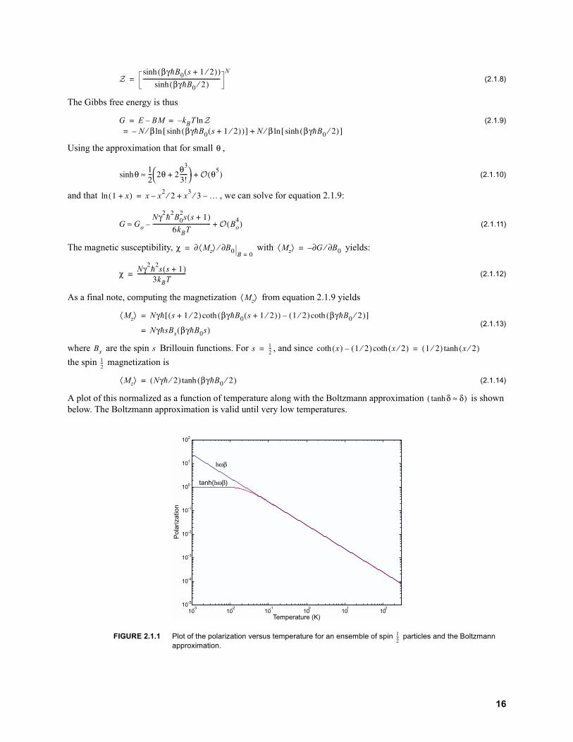
A plot of this normalized as a function of temperature along with the Boltzmann approximation is shown below. The Boltzmann approximation is valid until very low temperatures.
FIGURE 2.1.1 Plot of the polarization versus temperature for an ensemble of spin particles and the Boltzmann approximation.
βγ!B s ⁄( )( )
βγ!B ⁄( )-------------------------------------------------------
N
G E BM kBT
N β βγ!B s ⁄( )( )[ ]⁄ N β βγ!B ⁄( )[ ]⁄
θ
θ
--- θ
θ
-----
θ( )≈
x( ) x x⁄ x
⁄ …
G Go
Nγ!B
s s ( )
kBT----------------------------------------- Bo
( )≈
χ Mz⟨ ⟩∂ B∂⁄B
Mz⟨ ⟩ G∂ B∂⁄
χ Nγ!s s ( )kBT
----------------------------------
Mz⟨ ⟩
Mz⟨ ⟩ Nγ! s ⁄( ) βγ!B s ⁄( )( ) ⁄( ) βγ!B ⁄( )[ ]
Nγ!sBs βγ!Bs( )
Bs s s
--- x( ) ⁄( ) x ⁄( ) ⁄( ) x ⁄( )
---
Mz⟨ ⟩ Nγ! ⁄( ) βγ!B ⁄( )
δ δ≈( )
10-3
10-2
10-1
100
101
102
10-5
10-4
10-3
10-2
10-1
100
101
102
tanh(hωβ)
hωβ
Temperature (K)
Pol
ariz
atio
n
---
16

2.2 Nuclear Spin Dynamics of a Spin in a Static Field
We have seen from section 2.1 that a spin in a static z-directed flux density, gave energies that were eigenvalues of the component of spin . From equation 2.1.6, for a single spin, the time-dependent wave function is therefore
(2.2.1)
The most general solution is a linear superposition of the states
(2.2.2)
The expectation value for the magnetization is thus
(2.2.3)
Starting with the term, it is useful to redefine and in terms of the raising and lowering operators, and ,
, (2.2.4)
where (2.2.5)
Therefore unless . Solving for for a spin of ,
(2.2.6)
Since is the complex conjugate of , equation 2.2.6 can be rewritten as
(2.2.7)
It is convenient to express the normalization coefficients in terms of two real positive variables, and and two other real quantities and : and where giving
, where . (2.2.8)
Similarly, (2.2.9)
and (2.2.10)
This motion yields a classical picture of a vector making a fixed angle to the z-axis precessing in the x-y plane at the so called Larmor frequency. Consult [SLI96] for a more detailed discussion.
2.3 Spin Dynamics with a Rotating Magnetic Field
Consider a second magnetic field,
(2.3.1)
From the Schrödinger equation
(2.3.2)
As can be shown in appendix A, (2.3.3)
BoIz
ΨI m, t( ) ΨI m, e i !⁄( )mt
m
Ψ t( ) amm s
s
∑ ΨI m, e i !⁄( )mt
µµµµ t( )⟨ ⟩ Ψ t( ) µµµµΨ t( ) τd∫
γ!am′ am m′⟨ |
m m',∑ I m| ⟩e i !⁄( ) m ′ m( )t
µx Ix Iy I I
Ix
--- I I( ) Iy
i----- I I( )
IΨI m, I I ( ) m m ( ) ΨI m ,
IΨI m, I I ( ) m m ( ) ΨI m ,
m′⟨ |I±m| ⟩ m′ m± µx
---
µx t( )⟨ ⟩ γ! c ⁄ c ⁄
---⟨ |Ix
---| ⟩e iγB t c ⁄
c ⁄
---⟨ |Ix
---| ⟩eiγBt
[ ]
---⟨ |Ix
---| ⟩
---⟨ |Ix
---| ⟩
---
µx t( )⟨ ⟩ γ! c ⁄ c ⁄ e iγBt[ ]
a bα β c ⁄ aeiα c ⁄ beiβ a b
µx t( )⟨ ⟩ γ!ab α β ωt( ) ω γB
µy t( )⟨ ⟩ γ !ab α β ωt( )
µz t( )⟨ ⟩ γ! a b( ) ⁄
B t( ) zB xB ωzt yB ωz t
!i--- Ψ∂
t∂------- µµµµ B⋅ Ψ γ! BIz B Ix ωzt Iy ωzt( )[ ]
e iIzφ IxeiIzφ Ix φ Iy φ
17

Thus we obtain
(2.3.4)
It becomes easy to understand the evolution of by looking in the rotating frame
(2.3.5)
Therefore
(2.3.6)
Substituting this into equation 2.3.4 and multiplying the left of both sides by gives
(2.3.7)
The effects of the rotating field have now been removed. On resonance, yields
(2.3.8)
The dynamics are very similar to that of a static field–rotation about the x-axis. The final dynamics for the single spin magnetization expectation values are for
(2.3.9)
2.4 Product Operator Formalism
2.4.1 The Hamiltonian
The complete Hamiltonian for a nuclear spin is enormously complex, but one of the beautiful aspects of nuclear magnetic resonance is that the Hamiltonian can be reduced to a very simple one with a few phenomenological con-stants. The Hamiltonian is broken up into three parts:
(2.4.1)
The term is the Zeeman interaction, which is of the form for spins on a molecule
for a z-directed static field. (2.4.2)
The second term is the radio frequency field interaction, in the rotating frame of each spin is
(2.4.3)
The last term, is due to electron mediated nuclear spin-spin interactions of the form
(2.4.4)
In the weak coupling limit, , we can keep only one term of the scalar coupling
!i--- Ψ∂
t∂------- γ! BIz Be iIz ωztIxeiIzωz t
[ ]Ψ
Ψ
Ψ' eiωz tIzΨ
Ψ e i ωz tIzΨ'
Ψ∂t∂
------- iωzIz e i ωztIzΨ' e i ωz tIzΨ'∂t∂
--------
eiωzIz t
!i---
Ψ'∂t∂
-------- ! ωz γB( )Iz γ!BIx[ ]Ψ'
ωz γB
!i---
Ψ'∂t∂
-------- γ!BIxΨ'
γB ω
µz t( )⟨ ⟩ µz ( )⟨ ⟩ ωt µy ( )⟨ ⟩ ωt
µy t( )⟨ ⟩ µy ( )⟨ ⟩ ωt µz ( )⟨ ⟩ ωt
µx t( )⟨ ⟩ µx ( )⟨ ⟩
Z J
Z N
Z γIkzBk
N
∑ ωkIkzk
N
∑
B γk Ikx φ Iky φ( )k
N
∑
J
J π IkIlJklk l<∑
π Jkl
18

(2.4.5)
The full dipolar term and quadrupolar terms rarely show up in solution NMR since these interactions are averaged away by Brownian motion tumbling of the molecules.
2.4.2 The Reduced Density Matrix
From section 2.2 and on, it takes a lot of work to describe the evolution of the system. It would be nice to be able to use a compact formalism to describe spin dynamics. It is useful to look at the evolution of the density matrix. One can adapt the time-dependent Schrödinger equation for a wavefunction to the equation of motion of the density oper-ator.
(2.4.6)
This is the Louiville-von Neumann equation. This however describes the full dynamics of the whole system including space and spin degrees of freedom for electrons and nuclear spins. It is convenient to write the dynamics of just the reduced density operator, which according to [ERN87] yields the master equation
(2.4.7)
where the Hamiltonian acts only on the spins by tracing over all other degrees of freedom. is the equilibrium density operator. The term is a relaxation superoperator that exists in Louiville space. The Zeeman Hamiltonian, the Relaxation superoperator and the equilibrium density operator are all invariant under z-rotation transformations (to good approximation), and hence stay the same in the rotating frame.
If the terms of the density matrix are all arranged into a column vector of length , the master equation can be expressed in the form
(2.4.8)
If the Hamiltonian is time independent, this can be solved. When =0, , where is the steady state solution. Therefore this can be solved to yield
(2.4.9)
In general these equations are notoriously difficult to solve with relaxation. Ignoring relaxation, the time evolution of the density operator is
(2.4.10)
where . This can also be represented as a matrix multiplication. (2.4.11)
2.4.3 Product Operators
Since evolution is only a function of a single degree of freedom, , we can try to express the density operator in a complete set of orthogonal basis operators
(2.4.12)
These basis operators span a dimensional space known as a Louiville space. The expectation of an operator is
(2.4.13)
For pulse experiments, the basis that is chosen is based on the angular momentum operators , and . The com-plete list of product operators for spin for a two spin system are ( is the number of operators in the product)
J πJklIkzIlzk l<∑
t ρ t( ) i t( ) ρ t( ),[ ]
σs
t σs t( ) i s σs,[ ] Γ σs t( ) σ
s ρΓ
Γ
σσσσs n
t σσσσs isσσσσs Γ σΓ σΓ σΓ σs σσσσ( )
d dt⁄( )σσσσs is Γ( )σσσσ∞ Γσσσσ σσσσ∞
σσσσs σσσσ∞ e is ΓΓΓΓ( ) t σσσσ σσσσ∞( )
σσσσs t( ) R t( )σσσσ ( )R t( )
R t( ) ist( ) n n×
tBs
σ t( ) bss
n
∑ t( )Bs
n A
A⟨ ⟩ Aσ t( )
Ix Iy IzBs
--- q
19

(2.4.14)
The coherence order of each product operator is the sum of quantum numbers. For spins . The system in equilibrium starts at and only terms in the density operator with will be observed. One of the beau-tiful aspects of NMR is that all coherent orders can be observed with the application of specific pulses.
In general for N spin particles
(2.4.15)
which will yield 4N operators. is the index of the nucleus, = , or , and is the number of operators in the product. =1 for q spins and =0 for the remaining spins. Products of the cartesian operators are especially useful for a Hamiltonian whose terms all commute since the effects of the terms can just be evaluated in a cascade
(2.4.16)
Which is symbolically shown in Ernst’s arrow notation as(2.4.17)
Each of these corresponds to a rotation in the three-dimensional operator subspace. The evolution under the chemical shift terms and R.F. pulses cause rotations in single spin subspaces spanned by the operators . The cartesian rotation operator is
(2.4.18)
where and cyclic permutations thereof of an angle of rotation about the axis. Rotations are taken to be clockwise around the rotation vector (right hand rule). Scalar and dipolar coupling terms induce rota-tions within the following operator subspaces
(2.4.19)
The rotations in these subspaces is summarized in figure 2.4.1. As an example,
(2.4.20)
If the density operator contains products of operators for different spins, each operator transforms individually as shown in the example
(2.4.21)
Rotations of the subspace spanned by the remaining terms of the full scalar coupling will not be covered in this text.
q ---I I!" ( )
q Ix Iy Iz Ix IyIy,, , ,
q IxIx IxIy IxIx, ,
IyIx IyIy IyIz,,
IzIx IzIy IzIz,,
p N N p N≤ ≤p p ±
---
Bs q ( ) Ikα( )akq
k
N
∏
k α x y z qakq akq N q
σ t τ( ) iωkτIkz( ) iπJτIkzIlz( ) σ t( ) iπJτIkzIlz( )
k l<∏ iωkτIkz( )
k
∏k l<∏
k
∏
σ t( )ωτ IzωτIz…πJτIzIzπJτIzIz…σ t τ( )
Ikx Iky Ikz, ,( )
IkβφIkαIkβ φ Ikγ φ
α β γ, , x y z, , φ γ Bατ α
Ikx IkyIlz IkzIlz, ,( )
IkxIlz Iky IkzIlz, ,( )
Ilx IkzIly IkzIlz, ,( )
IkzIlx Ily IkzIlz, ,( )
IkyπJklτIkzIlzIky πJklτ( ) IkxIlz πJklτ( )
Ikα
IkβIlβ'φ'Ikα φ'Ilα'
Ikβ φ Ikγ φ( ) Ilβ' φ' Ilγ' φ'( )×
20

2.5 Decoherence
Little mention has been made of the relaxation superoperator, . The subject of decoherence is a difficult one, fraught with a lack of fundamental understanding of the processes involved when a system of interest couples to a bath and loses phase coherent information. The fact that molecular tumbling dramatically simplifies the Hamiltonian causes problems for fundamentally maintaining quantum coherence. Zeeman and interaction terms will all be slightly modulated by the tumbling of molecules and collisions cause information from molecules to diffuse about the lattice. In solids this is not as large of a problem, but permanent dipolar and quadrupolar coupling terms between nuclei on a molecule cause much faster relaxation rates than in liquids. Because of the difficulty of describing relaxation in quan-tum mechanics, NMR is usually described by the classical phenomenological Bloch equations. There are two relax-ation terms: , an irreversible longitudinal spin-lattice relaxation time where the system slowly relaxes to the equilibrium direction as information is slowly leaked to the lattice. This can be 10s of second in liquids and up to weeks in some solids; is the irreversible transverse spin-spin relaxation where inter– and intra–molecular spins become out of phase or randomized. is the loss of quantum coherence and is generally the parameter used to express the time one can compute quantum mechanically. The relation between the two relaxation mechanisms is
(2.5.1)
where is a positive valued function for all inputs. is temperature and is a vector of other parameters out of the realm of this discussion. The essence of this equation is that .
is the effective relaxation time including irreversible relaxation mechanisms, and reversible relaxation mechanisms such as inhomogeneity in the static field, applied gradient fields or radiation damping (back action from the coil due to Lenz’s Law). More will be mentioned in section 3.3. A simple equation is often used to relate the two [FUK81]:
(2.5.2)
The Bloch equations for the magnetization vector is
FIGURE 2.4.1 Product operator rotations within each subspace, reproduced from [ERN87].
ωkτ
Ikz
Ikx Iky
-Iky -Ikx
shift or z-Pulse
β
Ikz
Ikx
-Ikz
-Iky
Iky
β
Ikz
-Ikz
IkyIkx
-Ikx
x-Pulse y-Pulse
πJklτ
2IkzIlz
Ikx 2IkyIlz
-2IkyIlz -Ikx
πJklτ
2IkzIlz
2IkxIlz Iky
-Iky -2IkxIlz
coupling
Γ
Tz
TT
T-----
T----- f B T ξξξξ, ,( )
f T ξξξξT T≤
T T
T
------
T-----
T----- γ∆B
M t( )
21

(2.5.3)
where the relaxation matrix is
(2.5.4)
This form of the relaxation superoperator is only true in the absence of spin coupling [ERN87].
tM t( ) γM t( ) B t( )× R M t( ) M
R
R
T⁄
T⁄
T⁄
22

3.
NMR Spin Dynamics and Pulse Programming
3.1 Nuclear Spin Hamiltonians
The most common heteronuclear species for NMR are outlined in table 3.1.1.
Chemical shifts for most species are a few ppm of the resonance frequency. 13C and 19F shows larger variations – usually 100s of ppm. So far, the most commonly used species are protons and carbon – mainly due to the vast importance of organic molecules in chemistry, biology and technical applications. A second reason is that the cou-pling frequency can reach 100s of Hz, quite high for NMR. As will be shown later on, the approximate number of gates that can be implemented in a quantum computation without error correction is . The inverse of the coupling frequency is about the time that two gates can be implemented, as will be shown in section 4. One would like the J coupling frequencies to be as large as possible to allow more gates to be implemented within the quantum coherence time. In solids with full dipolar coupling, the coupling terms can be many kHz, but since the is much shorter in solids, the factor is much smaller, making them less effective computers. If the individual spins are iso-lated and manipulated, this opens up the possibility of quantum computation in the solid state [KAN98]. Liquid chlo-roform is a good example of a simple 2-bit quantum computer, used to perform a simple search algorithm [CHU98a].
The Hamiltonian for this species is [CHU98a]
(3.1.1)
Carbon-carbon couplings are quite small, and proton–proton couplings are exceedingly difficult to see [SCH98]. Fluorine coupling constants to both protons and carbon nuclei are good (100s to 10s of respectively) and fluorine–fluorine coupling constants are also reasonable . 19F–31P coupling frequencies over 1000Hz have been found [WEB72]. See [WEB72] for an exhaustive compilation of fluorine molecules and coupling con-stants. In general, it is difficult to find tabulated values of J-coupling since spectroscopists usually want information only about a homonuclear subspace and don’t want information from other heteronuclear species showing up in their
1H 2H (spin 1) 13C 15N 19F 31P
gyromagnetic ratio (rad T-1 s-1)
26.7510 x 10⁷ 4.1064 x 10⁷ 6.7263 x 10⁷ -2.7116 x 10⁷ 25.1665 x 10⁷ 10.8289 x 10⁷
naturalabundance
99.985% 0.015% 1.10% 0.37 100 100
sensitivity(relative to 1H)
1 9.65 x 10⁻³ 0.0159 0.0219 0.83 0.0663
TABLE 3.1.1 Tabulated values of the most common heteronuclear species used in NMR. 2H is used for linear control of the spectrometer (frequency, temperature, receiver stabilization).
FIGURE 3.1.1 chloroform, a prototypical molecule used for quantum computation.
J
TJ J
T
13C
1H
ClCl
Cl
B( ) πB × IHz × ICz( ) πIHzICz
Hz( )Hz
Hz( ) J
23

spectra. They use a variety of decoupling techniques to remove coherent evolution of the terms to get nice, simple spectra. This will be explained shortly.
3.2 Manipulating the Hamiltonian – Refocusing, Average Hamiltonian Theory
Consider the following pulse applied to a spin rotating in the transverse plane:
The evolution of this system can be analyzed completely with product operators, but this specific problem is more easily treated with commutators of cartesian operators. The evolution of the spin about the z-axis for a time is (let
) [MAT93] (see appendix A)
(3.2.1)
A rotation about the x-axis by 180° is represented by
(3.2.2)
The product of the two is
(3.2.3)
As can be verified for spin only, the cartesian rotation operators are anticommutative:
(3.2.4)
Therefore we can rewrite equation 3.2.3 as
(3.2.5)
For the scalar coupling term ( )
(3.2.6)
Since for applying the same techniques will yield
(3.2.7)
Amazingly this reverses the Hamiltonian evolution – it is just like time going backwards for the spin. This also works for pulses and where is an arbitrary axis in the transverse plane [MAT93]. This technique is known as refocusing – it allows one to change a Hamiltonian at will with R.F. pulses. It is useful for reducing reversible
effects such as spin interactions and inhomogeneity in the magnetic field. Repeated fast refocusing with coherent or incoherent R.F. sources is known as decoupling. It is routinely used in NMR spectroscopy to turn off interactions between heteronuclear spins. To a modern NMR spectroscopist or NMR quantum computing programmer, it is as important to do nothing as it is to do something – this ability in NMR is one of its best features.
FIGURE 3.2.1 A simple 180x pulse.
πJklIkzIlz
180x
τ τ
τωτ α
Rz iαIz( ) α---
i
α---
Iz
R#x iπIx( ) π---
iπ---
Ix iIx
R#xRz
iIxα---
i
α---
Iz
---
IxIy IyIx
IyIz IzIy
IyIz IzIy
R#xRz
α---
i
α--- Iz
iIx R z R#x
β πJτ
RJ iβIkzIlz( ) β---
iβ---
IkzIlz
Rkγ Rlβ,[ ] k l≠
Rkl#φRJ R J Rkl#φ
R#y R#φ φ
T
24

One might wonder how far can one go in manipulating Hamiltonians. Average Hamiltonian theory is the idea of representing the average of a Hamiltonian over a finite time from perturbative effects. It was introduced into NMR by John Waugh to explain multiple pulse experiments [ERN87]. The entire motion of during an interval can be described by a Hamiltonian , depending only on the boundary conditions if and only if:
1 The Hamiltonian is periodic (true for liquid NMR).2 Observations are made for a very short time and are synchronous with the Hamiltonian evolution.
3.3 Spin Echos and CPMG
From section 3.2, refocusing effects time-reversal of the Hamiltonian. This is true only in the absence of irrevers-ible spin-spin relaxation. From section 2.5 however, the relaxation time is reversible while relaxation persists. Through refocusing it seems possible to reverse the effects of spectral broadening. This was what Erwin Hahn discovered which essentially started the field of pulse NMR [SLI96]. Consider the spin echo pulse sequence below
From section 3.2, if there was no relaxation, the density operator at time using product operators would be , the same as it was after the pulse. Considering the effects of , let us presume the signal is a superposition
of signals from small volumes of spins resonating at slightly different frequency. For simplicity we assume that each microscopic volume contains a large amount of spins resonating at the same frequency, creating isochromats. Up until the so called pulse is applied, the spins become out of phase with each other, such that the free induction decay of nuclear spin magnetization detected by the coil decays with a time constant . The spins however are out of phase in a geometric way – no loss of information other than through irreversible relaxation.
Figure 3.3.2 shows two graphical means to understand the spin echo. The first plot shows the phase versus time of the spin echo, the second shows isochromatic spin vectors on the Bloch sphere. The isochromats begin to diverge causing
relaxation. After the pulse, the isochromats begin to converge again and finally meet at the -y axis a time later.
This is an interesting experiment because it shows how to measure information about the spin system for longer time scales than the inhomogeneity would allow. The Carr-Purcell sequence is essentially a spin echo followed by a long train of pulses spaced apart. This experiment allows one to measure the irreversible spin-spin coherence
FIGURE 3.3.1 The basic spin echo sequence demonstrating the different between reversible and irreversible coherence times.
FIGURE 3.3.2 Two different graphical ways to understand the spin echo. On the left is the angle versus time of isochromats in the transverse plane. On the right is the motion of spin vectors on the Bloch sphere.
t t t< < t t,( )
T T
T
180x
τ τ
90x
τIy Ix$ T
πT
T
Ix τ τ
180x90x
Iy
-Iy
x
y
z
T π τ
π τ
25
time since the only term that does not refocus is the relaxation time, . One simply measures the echo envelope at where .
It is difficult to create a perfect pulse and hence perform a Carr-Purcell sequence without accumulating large errors. Meiboom and Gill came up with a pulse sequence (CPMG) very similar to that of Carr and Purcell but made a few key changes. The first step is to alternate the phase of the pulses between the +x and -x–axis. The second, to introduced a phase shift with the first pulse. Meiboom and Gill were the first to show that these two changes would not accumulate errors–one could remove the systematic experimental error. The idea of creating perfect pulses out of imperfect ones has been extended with a beautiful group theoretic approach from Alex Pines [CHO85][FRE80].
3.4 2D Fourier Spectroscopy (COSY)
Two-dimensional techniques are an extremely powerful development. The idea of two-dimensional Fourier transformation is due to Jeener but it was Ernst who first fully appreciated the power of this method [SLI96]. The power of 2D correlation spectroscopy (COSY) is that it allows separation of terms in the Hamiltonian to determine properties of molecular systems. Chemical shifts can be fully distinguished from scalar coupling and the location of peaks on a 2D plot shows all the coupling relationships in a molecule. This ultimately allows one to begin to work backwards towards constructing a model for a particular molecule. This technique gives NMR unprecedented power to elucidate molecular structure in physics, biology, chemistry and medicine, supplanting techniques such as x-ray crystallography and IR spectroscopy.
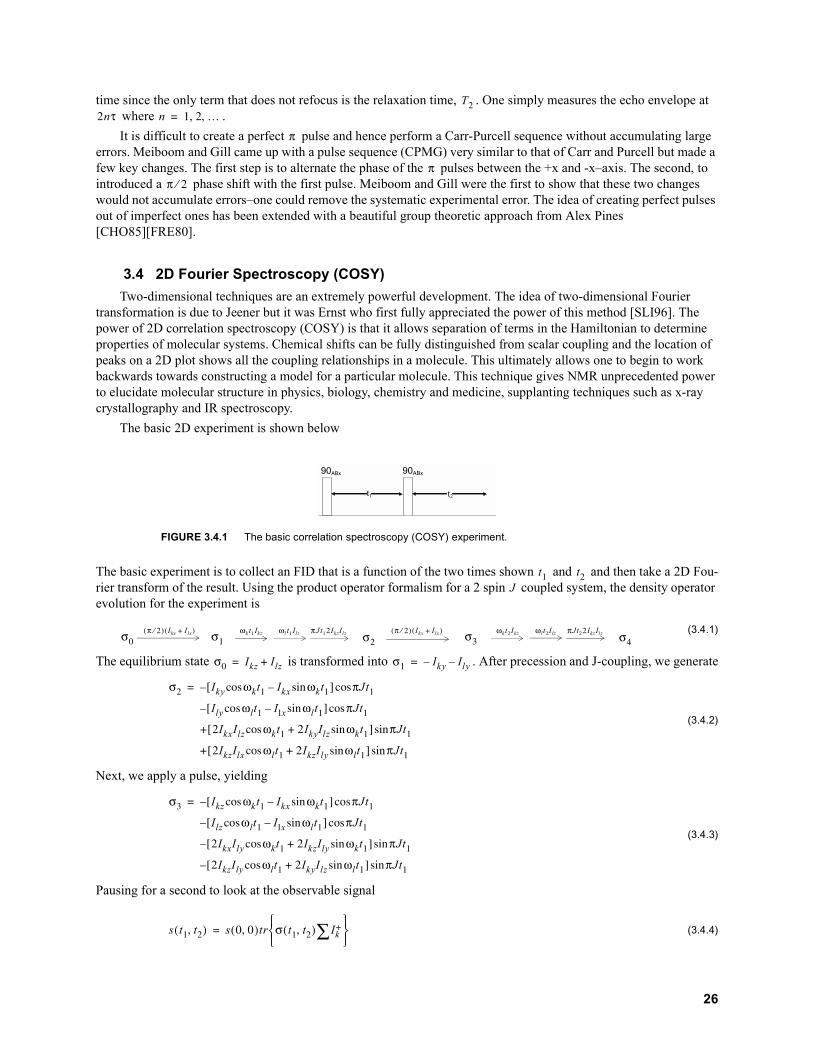
The basic 2D experiment is shown below
The basic experiment is to collect an FID that is a function of the two times shown and and then take a 2D Fou-rier transform of the result. Using the product operator formalism for a 2 spin coupled system, the density operator evolution for the experiment is
(3.4.1)
The equilibrium state is transformed into . After precession and J-coupling, we generate
(3.4.2)
Next, we apply a pulse, yielding
(3.4.3)
Pausing for a second to look at the observable signal
(3.4.4)
FIGURE 3.4.1 The basic correlation spectroscopy (COSY) experiment.
Tnτ n …, ,
π
ππ ⁄
90ABx
t1 t2
90ABx
t tJ
σ
π ⁄( ) Ikx Ilx( )σ
ωk tIkzωl tIlz πJtIkzIlzσ
π ⁄( ) Ikx Ilx( )σ
ωk tIkzωl tIlz πJtIkz Ilzσ
σ Ikz Ilz σ Iky Ily
σ Iky ωkt Ikx ωkt[ ] πJt
Ily ωlt Ix ωlt[ ] πJt
IkxIlz ωk t IkyIlz ωk t[ ] πJt
IkzIlx ωl t IkzIly ωl t[ ] πJt
σ Ikz ωkt Ikx ωkt[ ] πJt
Ilz ωlt Ix ωlt[ ] πJt
IkxIly ωk t IkzIly ωk t[ ] πJt
IkzIly ωl t IkyIlz ωl t[ ] πJt
s t t,( ) s ,( )tr σ t t,( ) Ik∑
26

Where , since we are detecting the spins with a quadrature detection system. Only terms with will be observable. Hence, the observable terms are
(3.4.5)
Again after chemical shift and -coupling evolution, we are left with the final state
(3.4.6)
The observable signal is thus (with relaxation)
(3.4.7)
Where . Taking the Fourier transform
(3.4.8)
for the function yields the complex Lorenztian peak
(3.4.9)
Where . Since and , there will be peaks at along the axis. Similarly, along the axis there will be peaks at . To put the entire signal on positive axes for both and , take the Cosine transform along the axis:
(3.4.10)
For a Cosine transform, signals that are antisymmetric about the origin of yield pure dispersive Lorentzians. Thus terms with add a modulation that yields in-phase dispersive signals
(3.4.11)
Terms symmetric about the origin yield pure absorptive Lorentzians. Terms with add a modu-lation that yields antiphase absorptive signals
(3.4.12)
The final results are summarized graphically in figure 3.4.2. Along the line is a normal dispersive 1D spec-trum of chemical shift and couplings together. In 2D, the -coupling terms cause off diagonal peaks to appear, sep-arating terms in the Hamiltonian. Peaks at the off diagonal axis, = , represent correlations between spins that leads to inference about molecular structure. For large molecules with complex conformations, 2D methods are extremely useful.
Ik Ikx iIky p
σobs Ikx ωkt πJt
Ix ωlt πJt
IkzIly ωk t πJt
IkyIlz ωl t πJt
J
σobs Ikx ωkt Iky ωk t[ ] ωkt πJt πJt
Ikx ωkt Iky ωk t[ ] ωlt πJt πJt
Ilx ωlt Ily ωl t[ ] ωlt πJt πJt
Ilx ωlt Ily ωl t[ ] ωkt πJt πJt
s t t,( ) eiωkte t t( )λ ωkt πJt πJt ωlt πJt πJt[ ]
eiωl te t t( )λ ωlt πJt πJt ωkt πJt πJt[ ]
λ T⁄
s t( )( ) S ω( ) s t( )eiωt
∞
∞
∫
eiωAte tλ
ZA ω( ) λλ ω ωA( )----------------------------------
i ω ωA( )
λ ω ωA( )----------------------------------
aA ω( ) idA ω( )
A k l, ωt eiωt eiωt( ) i⁄ ωt eiωt eiωt( ) ⁄ ωA J±ω ω ωA± J±
ω ω ω
c s t( )( ) s t( ) ωt td∞
∞∫ S ω( ) S ω( )
------------------------------------
ω
ωAt πJt πJt
sAid ω ω,( ) dA ω J( ) dA ω J( )[ ] dA ω J( ) dA ω J( )[ ]
ωAt π Jt πJt
sAaa ω ω,( ) aA ω J( ) aA ω J( )[ ] aA ω J( ) aA ω J( )[ ]
ω ω
J Jω ω,( ) ωk ωl,( ) ωl ωk,( )
27

FIGURE 3.4.2 Correlation spectroscopy (COSY) plot for two coupled heteronuclear spins showing chemical shift evolution separated from -coupling.
main diagonal
ω1
ω2
J
28

4.
Quantum Computing
4.1 Qubit
A qubit or quantum bit is a system which exists in a two level Hilbert space and is capable of being in a superpo-sition of its Boolean states. qubits are able to exist in a dimensional Hilbert space.
4.2 Universal Computation
A universal quantum computer is a device capable of applying any unitary matrix with arbitrary accuracy to a set of qubits. What is are the requirements of a universal quantum computer? Fundamentally there are four basic require-ments [CHU98b].
1 The first is the ability to start in a known state (a pure state such as the ground state).2 To be able to efficiently perform any unitary transform with a set of elementary unitary transformations.3 Possess enough quantum coherence time to be able to perform any unitary transform.4 Make a measurement of the quantum state to read out the computational result.
Let us deal with the first point later on in the text. Regarding the second and third point: ultimately one would like to make a machine that can apply any unitary operator. This unitary operator is the computational function one is interested in computing. In classical, digital, irreversible computing, a single 2-bit gate, the NAND, applied to pairs of bits of any length string is capable of representing any function mapping one string to another. Quantum computers cannot use this specific gate since quantum mechanics is reversible. For a Hermitian matrix,
(4.2.1)
Therefore an inverse always exists. Irreversible operators like the NAND gate cannot be simulated. Even for classical reversible computers, the NAND gate is insufficient [BEN85]. Fredkin and Toffoli showed a three bit gate [FRE82] is the reversible analog of the NAND gate, but no two-bit gates exist. In quantum computing, it was shown that this Tof-foli gate and arbitrary single qubit rotations were enough to be a universal family of unitary operators [DEU89]. Arbi-trary single qubit rotations are necessary since a unitary matrix can contain complex numbers as opposed to just the elements of the set 0, 1 in classical, digital computers. [BAR95b] has shown that matrices in the computational basis of the form
(4.2.2)
are universal. , and are irrational multiples of and each other. Repeated application interspersed with rota-tion operators are sufficient to describe any unitary operator acting on bits. These constraints were relaxed signifi-cantly when [LLO95] and [DEU95] showed that almost any 2-bit gate with arbitrary rotations is universal. In quantum computing, a common gate is called the CNOTa,b. For a state , this gate conditionally flips the state of if and does nothing if . As a matrix in the computational basis it is represented as
N N
U U%
U α φ θ, ,( )
eiα θ iei α φ( ) θ
iei α φ( ) θ eiα θ
α θ φ πN
ab| ⟩ ba a
29
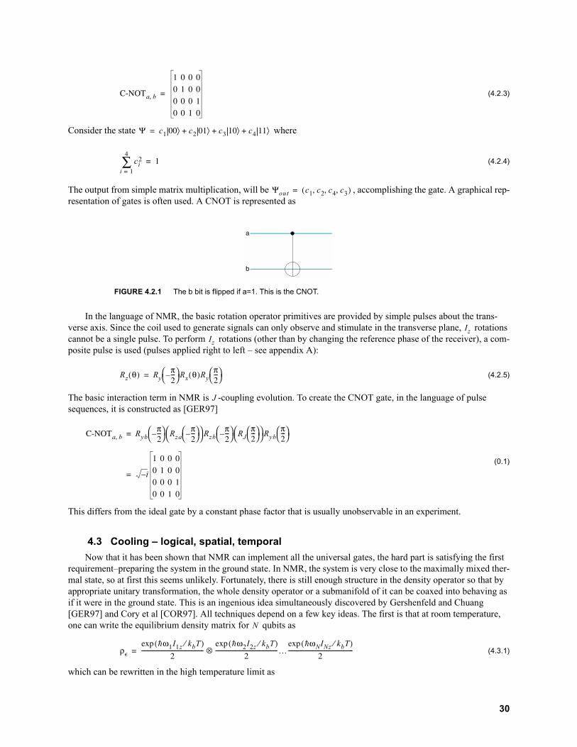
(4.2.3)
Consider the state where
(4.2.4)
The output from simple matrix multiplication, will be , accomplishing the gate. A graphical rep-resentation of gates is often used. A CNOT is represented as
In the language of NMR, the basic rotation operator primitives are provided by simple pulses about the trans-verse axis. Since the coil used to generate signals can only observe and stimulate in the transverse plane, rotations cannot be a single pulse. To perform rotations (other than by changing the reference phase of the receiver), a com-posite pulse is used (pulses applied right to left – see appendix A):
(4.2.5)
The basic interaction term in NMR is -coupling evolution. To create the CNOT gate, in the language of pulse sequences, it is constructed as [GER97]
(0.1)
This differs from the ideal gate by a constant phase factor that is usually unobservable in an experiment.
4.3 Cooling – logical, spatial, temporal
Now that it has been shown that NMR can implement all the universal gates, the hard part is satisfying the first requirement–preparing the system in the ground state. In NMR, the system is very close to the maximally mixed ther-mal state, so at first this seems unlikely. Fortunately, there is still enough structure in the density operator so that by appropriate unitary transformation, the whole density operator or a submanifold of it can be coaxed into behaving as if it were in the ground state. This is an ingenious idea simultaneously discovered by Gershenfeld and Chuang [GER97] and Cory et al [COR97]. All techniques depend on a few key ideas. The first is that at room temperature, one can write the equilibrium density matrix for qubits as
(4.3.1)
which can be rewritten in the high temperature limit as
FIGURE 4.2.1 The b bit is flipped if a=1. This is the CNOT.
&'()a b,
Ψ c | ⟩ c | ⟩ c | ⟩ c | ⟩
ci
i
∑
Ψout c c c c, , ,( )
a
b
IzIz
Rz θ( ) Ryπ---
Rx θ( )Ryπ---
J
&'()a b, Rybπ---
Rzaπ---
Rzb
π---
RJπ---
Ryb
π---
i
N
ρ
!ωIz kbT⁄( )
--------------------------------------------
!ωIz kbT⁄( )
--------------------------------------------⊗ …
!ωNINz kbT⁄( )
----------------------------------------------
30

(4.3.2)
where and is the deviation density matrix. Since , an arbitrary unitary transform on
(4.3.3)
Thus, since only the deviation density matrix is observable (with the appropriate pulses), we can ignore the identity term and focus attention on the deviation density matrix only.
Also note that if the diagonal of the deviation density matrix is of the form
(4.3.4)
where , the result of a computation will be just as if one acted on a pure state. This is because one could subtract off a factor that would only leave the effective pure state in the deviation density matrix [GER97].
There are essentially three types of preparation types:
1 logical labelling [GER97], where ancilla spin allow the creation of submanifolds which behave like pure states but the Von-Neumann entropy of the overall density matrix is unchanged. Consider a three spin system to distill 2 qubits which have for . The diagonal of the deviation density matrix is [VAN99]
(4.3.5)
Consider the state
(4.3.6)
This is accomplished by two commuting operators: and . Looking at the first four ele-ments of the density matrix, this is a effective pure state conditioned on the first bit being 0. Hence, a computational result is conditioned on the state of the ancilla. By performing two experiments and post-appending the second by two CNOT gates, the unwanted signal can be subtracted out. It is important that the state of the ancilla qubits do not change during the experiment, so refocusing is done. The generaliza-tion of this procedure requires a modular addition transform which can be implemented with the unitary Fourier transform and rotations about the -axis. Consult [CHU98b] for a more detailed discussion.
2 Spatial labelling [COR97], where macroscopically nonunitary static field gradients are applied to a sam-ple creating a series of parallel running computations. The effect of a gradient on a small isochromat is unitary, but since the gradient can dephase different isochromats, there is no observable magnetization of unwanted components in the transverse plane. Gradients commute with the , and product operators, and since a effective pure state is
(4.3.7)
Subtracting a factor yields the effective ground state. To create this state requires creating single and double quantum coherences that are dephased out by the gradients [COR98].
3 Temporal labelling [KNI97], encompasses a variety of techniques based on randomization such that averaging over a number of experiments produces a pseudo-pure state. This technique is very efficient
ρ
αIz
----------------------
αIz
----------------------⊗ …
αNINz
------------------------
N------ ρ∆
αi
!ωi
kbT--------- ρ∆ UU% ρ
UρU% U
N------U% Uρ∆U%
N------ Uρ∆U%
ρ∆ β δ δ … δ, , ,( )
δ β N ( )⁄
δ
ωi ω i , ,
↓↓↓ ↓↓↑ ↓↑↓ ↓↑↑ ↑↓↓ ↑↓↑ ↑↑↓ ↑↑↑α α α α α α α α
↓↓↓ ↑↓↑ ↑↑↓ ↓↑↑ ↑↓↓ ↓↓↑ ↓↑↓ ↑↑↑α α α α α α α α
&'() &'()
z
Ikz Ilz IkzIlz
Ikz
------
Ilz
----- IkzIlz
⁄
⁄
⁄
⁄
⁄
31

for small number of qubits, requiring no ancilla and no gradients. Consider the thermal equilibrium devi-ation density matrix
(4.3.8)
Applying operators that cyclically permute populations for 2 experiments such that
, (4.3.9)
Averaging the three experiments and subtracting the term yield
(4.3.10)
An effective ground state. This is accomplished by the operator
(4.3.11)
The algorithm is
(4.3.12)
Other methods for temporal labelling can be found in [KNI97].
It is important to note that of these methods cause the detected signal to decrease exponentially with the size of the computer. This has dire consequences to Boltzmann bulk NMR quantum computing as will be outlined in section 12.
4.4 Readout
Readout is the last nontrivial aspect to allow NMR to implement bulk quantum computing. One needs to be able to make measurements in the computational basis, unobservable in NMR. A measurement is
(4.4.1)
The way around this, as will be described later, is to apply pulses which move elements of the density matrix to observable transverse magnetization. As will be shown, it is possible to do state tomography of the entire density matrix.
A second problem is that some quantum algorithms, such as Shor’s prime factorization algorithm produces a ran-dom output. Averages over the ensemble could produce a null result. Gershenfeld and Chuang show how to make probabilistic algorithms deterministic by making the system perform a classical computation on some statistic and then read out the mean value of an answer bit by bit with a polynomial slowdown [GER97].
ρ∆
ρ∆
ρ∆
ρ∆*
P
P
ρ∆ P ρ∆P
ρ∆ Pρ∆P
s t t,( ) s ,( )tr σ∆ t t,( ) Ik∑
32

5.
RF Design
5.1 Introduction
The last three chapters considered the theoretical approaches to NMR and quantum computing. This chapter is the last in the series of introductory chapters necessary to understand the hardware development ideas that will follow in the rest of this thesis. It makes a marked jump from physics to RF engineering, critical to the development of good NMR spectrometers. The Larmor frequency of spins at ranges from about 5 MHz to about 50 MHz, thus a good understanding of the methods, tools and circuits used in RF design facilitate the understanding of NMR probes for transmitting and receiving signals (Chapter 6) and then the actual transmit, receive and switch modules (Chapter 10).
5.2 RF Spectrum
The RF spectrum is shown below in figure 5.2.1. For this project, the range of frequencies is about 5-80 MHz, HF to VHF frequencies. In this range, the wavelength of radiation is much larger than the scale of the components used for constructing the RF electronics.
5.3 2 Port Networks and Impedance Matching
In RF design, one must be careful to match the port impedance of the probe to maximize power transfer. This can be proved by considering a voltage source with resistive source impedance and a resistive load impedance of
, as shown in figure 5.3.1.
The power in the load resistance is:
(5.3.1)
Now, to maximize power transfer, differentiate with respect to :
FIGURE 5.2.1 The RF spectrum.
FIGURE 5.3.1 Simple circuit used for power transfer analysis.
T( )
VLF LF MF HF VHF UHF SHF EHF9 kHz 30 kHz 30 MHz300 kHz 3 MHz 300 MHz 3 GHz 30 GHz 300 GHz
33 km 10 km 1 km 100 m 10 m 1m 100 mm 10 mm 1 mm
VS rsRL
rs
+- RLVs
PRL
RL
rS RL( )-------------------------VS
RL
33

(5.3.2)
Which implies that maximum power is delivered when .
To be complete, the second derivative is:
(5.3.3)
proving this is indeed a maximum for .
5.3.1 Transmission Lines
At RF frequencies when wires begin to present non-trivial reactances, it is important to understand the matching with a transmission line. For the circuit shown in figure 5.3.2, the input impedance looking into the transmission line from the generator end is
(5.3.4)
where , and is the wavelength of the electromagnetic energy in the coaxial cable [POZ90]. The function is a highly nonlinear function. To make circuit design easy and not have severe generator load mismatches in a
circuit, if , , and maximal power transfer is guaranteed. If , load mismatches start to become problematic if at even , so for frequencies above 2-5 MHz, impedances should always be matched.
5.3.2 S-Parameters
For an 2 port network, the ratio of the incident and reflected voltages can be related by the matrix
(5.3.5)
The matrix of values gives a measure of the reflection and transmission coefficients of a system. This is mea-surable on instruments known as vector network analyzers and are an essential tool for the RF designer. Many RF components give the scattering matrix so that systems can be cascaded to calculate performance. This can easy be generalized to more ports.
FIGURE 5.3.2 Measuring power transfer with a coaxial line of impedance .
PddRL---------
VS
rS RL( )-------------------------
VSRL
rS RL( )-------------------------
RL rS
dP
RLd ------------
VS
rS RL( )-------------------------
RLVS
rS RL( )------------------------- ≤
RL rS
Zin ZZl jZ βl
Z jZl βl---------------------------------
Zin
Zg
Z0,β Zl
Γ
Vg
Z
β πλ
------ λθ
Zl Z Zin Z Zl Z≠l λ ⁄
V
V
S SS S
V
V
S
34

5.3.3 Impedance Transformation Networks
It is useful in a variety of circumstances to be able to transform impedances for impedance matching and other techniques. The first transformation is a shunt to series capacitor transformation depicted in figure 5.3.3.
The impedance looking into the series combination is
(5.3.6)
The reciprocal of the impedance, the admittance, is always of the form where is the reciprocal of the parallel resistance and is the reciprocal of the parallel reactance. From equation 5.3.6, the admittance is
(5.3.7)
Therefore, the equivalent parallel resistance is
(5.3.8)
It is often needed for impedance transformation networks to know the capacitance required to transform into a desired resistance . This capacitance is
(5.3.9)
The parallel capacitance is
(5.3.10)
for most reasonable impedance transformations.
For a shunt to series capacitor transformation shown in figure 5.3.4, the impedance looking in is
(5.3.11)
The equivalent series resistance is therefore
FIGURE 5.3.3 Transforming a shunt configuration of a resistor and capacitor on the left to a series pair on the right.
FIGURE 5.3.4 Transforming a series configuration of a resistor and capacitor on the left to a shunt pair on the right.
Rs
Cs
Z
R0 C
Z
Z s( )
sC------ R
Y s( ) Y G iB GB
Y s( )ω
CR jωC
ωCR
-------------------------------------
Rs
ωCR
ωCR
------------------------------
RpR
C
ω RpR R( ) ⁄
------------------------------------------
CpC
ωRC
------------------------------ C≅
Z s( ) R sRC--------------------
R0
C
Z
Rp Cp
Z
35

(5.3.12)
The capacitor required to transform into is
(5.3.13)
The equivalent series capacitance is
(5.3.14)
5.4 Decibels, Gain and Power
In RF design, gain is usually expressed in dB. For power delivered to a load from a source peak voltage, , the gain is
(5.4.1)
where is the power delivered to the load and is the power available from the source. If the load and source impedances are the same, the gain can be expressed as
(5.4.2)
where is the load peak voltage.
It is often convenient to express power in absolute units of dB. The most common is the dBm, the power in dB relative to 1 mW. Another convenient unit is the dBc, the relative power of a signal to a carrier peak of interest in the frequency spectrum.
5.5 The Smith Chart
The Smith Chart was invented by Philip H. Smith in 1939 [HAY96][BOW82]. It has become an invaluable tool for engineers and scientists to understand complicated networks of resistances and reactances in a graphical means. See [BOW82] for a good, concise explanation of the Smith chart, shown in figure 5.5.1. It is essentially a polar plot of the normalized reflection coefficient,
(5.5.1)
where is the complex network impedance of the form . If the normalized reflection coefficient is expressed in polar form in a rectangular coordinate system,
(5.5.2)
Then a series of circle acting as constraint equations are generated:
(5.5.3)
describes a family of constant resistance circles while
(5.5.4)
Rs
R
ωCR
------------------------------
Rs R
C
ω----
R Rs( ) ⁄
R
------------------------------
Cs
ωRC
ωCR
------------------------------
RL Vs
G PL Ps⁄( )
PL Ps
G VL Vs⁄( )
VL
Γ S
ΓZ
Z ---------------
Z R jX
Γ p jq
pR
R -------------
q
R -------------
p ( ) q
X---
X---
36

describes a family of constant reactance arcs, shown in figure 5.5.1.
All arcs above the centerline of the chart represent or inductive reactances and all arcs below the centerline rep-resent of capacitive reactances. To plot a normalized series impedance value , one simply finds the intersection of the R=constant and X=constant circles. To find the admittance of an impedance, one simply measures the distance from the impedance to the point , and then draws the same length line to a point opposite from the original point. This point is the admittance. These examples are shown in figure 5.5.1
To find the input impedance of a general network, adding a series capacitor to an impedance means going counterclockwise on the constant resistance curve from the intersecting constant reac-
tance curve to the curve . A series inductor means going clockwise instead. A shunt capacitor requires going clockwise on an admittance Smith Chart: simply perform an admittance transformation and go through the same steps in a clockwise fashion as for the series capacitor. A shunt inductor is the same except in a counterclockwise configu-ration. One simply keeps adding shunt and series components and the final point on the impedance Smith chart will yield the final input impedance. A summary of these ideas is shown in figure 5.5.2.
FIGURE 5.5.1 The canonical Smith chart. showing a constant resistance and a constant reactance circle. Also shown is an impedance to admittance transformation simply by drawing a line through the origin.
0.1
0.1
0.1
0.2
0.2
0.2
0.3
0.3
0.3
0.4
0.4
0.4
0.50.5
0.5
0.6
0.6
0.6
0.7
0.7
0.7
0.8
0.8
0.8
0.9
0.9
0.9
1.0
1.0
1.0
1.2
1.2
1.2
1.4
1.4
1.4
1.6
1.6
1.6
1.8
1.8
1.8
2.02.0
2.0
3.0
3.0
3.0
4.0
4.0
4.0
5.0
5.0
5.0
10
10
10
20
20
20
50
50
50
0.2
0.2
0.2
0.2
0.4
0.4
0.4
0.4
0.6
0.6
0.6
0.6
0.8
0.8
0.8
0.8
1.0
1.0
1.01.0
20-20
30-30
40-40
50
-50
60
-60
70
-70
80
-80
90
-90
100
-100
110
-110
120
-120
130
-130
140
-140
150
-150
160
-160
170
-170
180
±
90-9
085
-85
80-8
0
75-7
5
70-7
0
65-6
5
60-6
0
55-5
5
50-5
0
45
-45
40
-40
35
-35
30
-30
25
-25
20
-20
15
-15
10
-10
0.04
0.04
0.05
0.05
0.06
0.06
0.07
0.07
0.08
0.08
0.09
0.09
0.1
0.1
0.11
0.11
0.12
0.12
0.13
0.13
0.14
0.14
0.15
0.15
0.16
0.16
0.17
0.17
0.18
0.18
0.190.19
0.20.2
0.210.21
0.22
0.220.23
0.230.24
0.24
0.25
0.25
0.26
0.26
0.27
0.27
0.28
0.28
0.29
0.29
0.3
0.3
0.31
0.31
0.32
0.32
0.33
0.33
0.34
0.34
0.35
0.35
0.36
0.36
0.37
0.37
0.38
0.38
0.39
0.39
0.4
0.4
0.41
0.41
0.42
0.42
0.43
0.43
0.44
0.44
0.45
0.45
0.46
0.46
0.47
0.47
0.48
0.48
0.49
0.49
0.0
0.0
AN
GLE O
F TRA
NSM
ISSION
CO
EFFIC
IENT IN
DEG
REES
AN
GLE O
F REFL
EC
TIO
N C
OE
FFICIE
NT
IN D
EGR
EES
Ð>
WA
VEL
ENG
THS
TOW
AR
D G
ENER
ATO
R Ð
><Ð
WA
VEL
ENG
THS
TOW
AR
D L
OA
D <
Ð
IND
UC
TIV
E R
EAC
TAN
CE
COM
PON
ENT (+
jX/Zo), O
R CAPACITIVE SUSCEPTANCE (+jB/Yo)
CAPACITIVE REACTANCE COMPONENT (-jX
/Zo), O
R IND
UCTI
VE
SUSC
EPTA
NC
E (-
jB/Y
o)
RESISTANCE COMPONENT (R/Zo), OR CONDUCTANCE COMPONENT (G/Yo)
constantresistancecircle
constant reactancearc
Z=1+j1
Y=0.5-0.5j
jXjX Z R jX
j
C jS
Z R jX RX X S
37

5.6 Q for a Lossy Inductor in a LC resonator
The definition of is:
(5.6.1)
where is the width at half maximum height. is also defined as:
(5.6.2)
For an electromagnetic wave, energy oscillates between magnetic and electric. The loss per cycle is purely ohmic, so considering the magnetic cycle:
(5.6.3)
For a series capacitor, it can readily be verified that . This resistance is a series resistance. In the mega-hertz to gigahertz range of NMR, inductors are by far the most lossy elements: they possess 's on the order of 10-100, compared to 500-5000 for capacitors. is a definition for a resonant circuit, so the for a single reactive com-ponent is defined as the of a circuit with the lossy component resonated with an ideal lossless reactance. For a stan-dard coil, the inductance of a coil is defined as:
(5.6.4)
where is the magnetic flux through turns of loop and is the current going through the loop. For a standard turn cylindrical coil, the flux through the cross sectional area of the coil, is:
FIGURE 5.5.2 Impedance and admittance Smith charts to allow one to find the input impedance or admittance of any linear network without performing any calculations.
series C shunt C
shunt Lseries L
Q
Qfo
δf dB
---------------
δf dB Q
Q π+"!",+" "
------------------------------------------------------------------
+"!", iL ⁄
+" " iRs f⁄
Q∴ ωLRs-------
Q ωCRs⁄
QQ Q
Q
LNφi
-------
Φ N i N
38
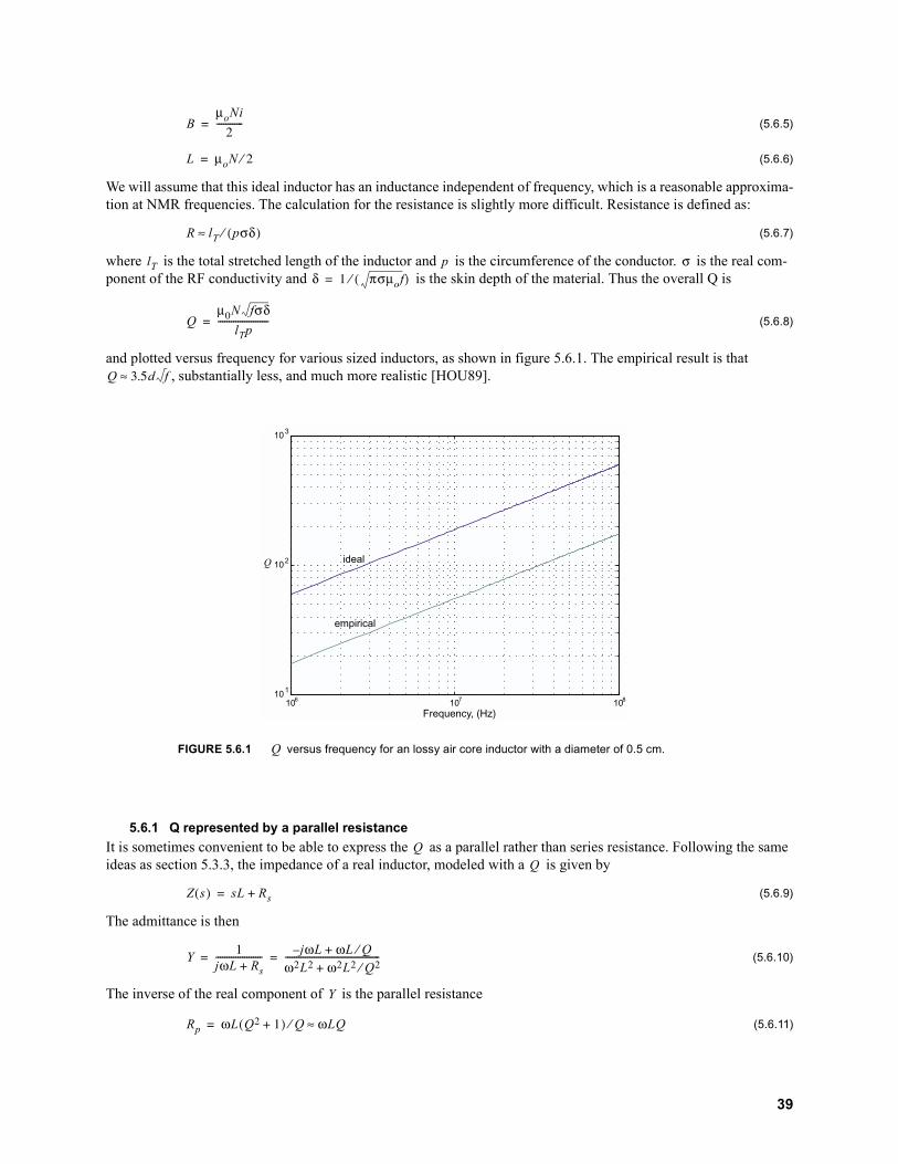
(5.6.5)
(5.6.6)
We will assume that this ideal inductor has an inductance independent of frequency, which is a reasonable approxima-tion at NMR frequencies. The calculation for the resistance is slightly more difficult. Resistance is defined as:
(5.6.7)
where is the total stretched length of the inductor and is the circumference of the conductor. is the real com-ponent of the RF conductivity and is the skin depth of the material. Thus the overall Q is
(5.6.8)
and plotted versus frequency for various sized inductors, as shown in figure 5.6.1. The empirical result is that , substantially less, and much more realistic [HOU89].
5.6.1 Q represented by a parallel resistance
It is sometimes convenient to be able to express the as a parallel rather than series resistance. Following the same ideas as section 5.3.3, the impedance of a real inductor, modeled with a is given by
(5.6.9)
The admittance is then
(5.6.10)
The inverse of the real component of is the parallel resistance
(5.6.11)
FIGURE 5.6.1 versus frequency for an lossy air core inductor with a diameter of 0.5 cm.
BµoNi
------------
L µoN ⁄
R lT pσδ( )⁄≈
lT p σδ πσµof( )⁄
QµN fσδ
lTp-----------------------
Q d f≈
Q
106 107 108101
102
103
Frequency, (Hz)
Q ideal
empirical
Z s( ) sL Rs
Y
jωL Rs--------------------- j ωL ωL Q⁄
ωL ωL Q⁄-------------------------------------------
Y
Rp ωL Q ( ) Q⁄ ωLQ≈
39
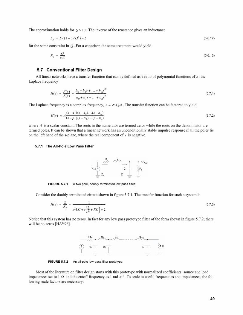
The approximation holds for . The inverse of the reactance gives an inductance
(5.6.12)
for the same constraint in . For a capacitor, the same treatment would yield
(5.6.13)
5.7 Conventional Filter Design
All linear networks have a transfer function that can be defined as a ratio of polynomial functions of , the Laplace frequency
(5.7.1)
The Laplace frequency is a complex frequency, . The transfer function can be factored to yield
(5.7.2)
where is a scalar constant. The roots in the numerator are termed zeros while the roots on the denominator are termed poles. It can be shown that a linear network has an unconditionally stable impulse response if all the poles lie on the left hand of the s-plane, where the real component of is negative.
5.7.1 The All-Pole Low Pass Filter
Consider the doubly-terminated circuit shown in figure 5.7.1. The transfer function for such a system is
(5.7.3)
Notice that this system has no zeros. In fact for any low pass prototype filter of the form shown in figure 5.7.2, there will be no zeros [HAY96].
Most of the literature on filter design starts with this prototype with normalized coefficients: source and load impedances set to 1 and the cutoff frequency as 1 rad . To scale to useful frequencies and impedances, the fol-lowing scale factors are necessary:
FIGURE 5.7.1 A two pole, doubly terminated low pass filter.
FIGURE 5.7.2 An all-pole low-pass filter prototype.
Q >
Lp L Q⁄( )⁄ L≈
Q
RpQ
ωC--------
s
H s( ) P s( )Z s( )-----------
b bs … bmsm
a as … ansn
---------------------------------------------------
s σ jω
H s( ) As z( ) s z( )… s zm( )s p( ) s p( )… s pn( )
---------------------------------------------------------------
A
s
Rl+-
Rs
Vs C
L
ZT Z
Vout
H s( ) ZZT------
sLC sLR--- RC
-------------------------------------------------------
1 Ω+-
1 Ω g2
g1 g3 gn
g4 gn-1
Ω s
40

(5.7.4)
For a high pass filter, since everything is normalized, all one has to do is move shunt impedances to series and vice versa and take the inverse of all the values
(5.7.5)
For a band pass filter, one creates a low pass prototype with set as the bandwidth, of the passband. Then one resonates each component at the geometric mean of the two edges of the passband, and
(5.7.6)
In filter design there is no such thing as an ideal filter: a perfect brick wall filter has a horrible impulse response, detrimental to pulsed applications like NMR. One must always make frequency-time tradeoffs, and the filters that have emerged in practice are those which make the most reasonable tradeoffs to be useful. For the NMR system designs to follow, high stopband attenuation is important. However, one must be careful of the tradeoff seen with the brick wall filter: for large stopband rejection, the phase performance in the passband becomes very nonlinear. For all pulsed applications in general, the phase performance in the passband of the filter must be reasonably linear so that the group delay for a pulse is constant.
(5.7.7)
Otherwise the pulse will be severely distorted. The two most common all-pole filters in practice are the Butterworth and Chebyshev, outlined below
5.7.2 Butterworth Response
The simplest filter is the normalized Butterworth response:
(5.7.8)
where n is the degree of the polynomial and is also the number of components required. A plot of the amplitude-fre-quency response for various values of is shown in figure 5.7.3.
From this plot, it is readily apparent that the passband is maximally flat, with reasonable attenuation in the stop-band and reasonable phase performance in the passband. From this frequency response, the pole locations in the s plane are [HAY96]
(5.7.9)
Since the pole locations are described by sine and cosine functions of the same argument, the Butterworth filter poles all lie on the unit circle of the s-plane. The parameter of the transfer function, . The filter values for load and source impedances of 1 are given by
(5.7.10)
Ck
gk
Rωc-------------
Lk
gkR
ωc-----------
gk
Ck
gkRωc------------------
Lk
R
gkωc
------------
ωc ∆ωflo fhi
fc flofhi
tg θ( ) dθdω-------
H jω( )
ωn( ) ⁄-------------------------------
n
sk i k ( ) πn------ i
π---
k … n, , , ,( )
A
Ω
gk k ( ) πn------
41

5.7.3 Chebyshev Response
The Chebyshev response is rarely expressed in closed form since the representation is more complex. In the s-plane, the poles are located on hyperbolic contours. The frequency response is given by
(5.7.11)
where is the Chebyshev polynomial defined by
(5.7.12)
and the parameter is the passband ripple given by
(5.7.13)
A is the depth of the ripple in dB. A plot of the ripple characteristics for several values is shown in figure 5.7.4. From this plot, it is apparent there is a strong tradeoff between passband ripple and stopband rejection. A plot of the Cheby-shev response is shown in figure 5.7.5. Notice that the stopband rejection of this plot is better than the Butterworth for equal order. However, this is at the expense of slightly worse phase performance, but still linear with small higher order contributions.
To calculate the poles, the following set of equations are required (these may seem somewhat arbitrary but come from the closed form solution):
(5.7.14)
where (5.7.15)
To then calculate the values, first calculate
FIGURE 5.7.3 |S12| and angle versus frequency for the Butterworth filter for various polynomial orders. The phase plot is constrained between and . Unravelled, the plot would be continuous.
0 0.5 1 1.5 2 2.5 3-4
-3
-2
-1
0
1
2
3
4
n=3
5
7
phase(rad)
frequency, (rad s-1)0 0.5 1 1.5 2 2.5 3
-35
-30
-25
-20
-15
-10
-5
0
frequency, (rad s-1)
n=3
5
7
|S12|(dB)
π π
H jw( )
Cn ω( )[ ] ⁄
-------------------------------------------
Cn ω( )
Cn ω( ) n ω ( ) ω <
Cn ω( ) n ω ( ) ω >
A
sk N k ( ) πn------
j N k ( ) πn------
N
n---
---
gk
42
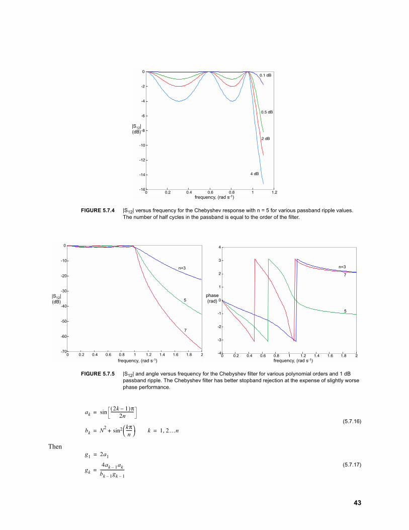
(5.7.16)
Then
(5.7.17)
FIGURE 5.7.4 |S12| versus frequency for the Chebyshev response with n = 5 for various passband ripple values. The number of half cycles in the passband is equal to the order of the filter.
FIGURE 5.7.5 |S12| and angle versus frequency for the Chebyshev filter for various polynomial orders and 1 dB passband ripple. The Chebyshev filter has better stopband rejection at the expense of slightly worse phase performance.
0 0.2 0.4 0.6 0.8 1 1.2-16
-14
-12
-10
-8
-6
-4
-2
0
frequency, (rad s-1)
|S12|(dB)
0.1 dB
0.5 dB
2 dB
4 dB
0 0.2 0.4 0.6 0.8 1 1.2 1.4 1.6 1.8 2-70
-60
-50
-40
-30
-20
-10
0
frequency, (rad s-1)
|S12|(dB)
n=3
5
7
0 0.2 0.4 0.6 0.8 1 1.2 1.4 1.6 1.8 2-4
-3
-2
-1
0
1
2
3
4
n=3
5
7
phase(rad)
frequency, (rad s-1)
akk ( )πn
-----------------------
bk N kπ
n------
k …n,
g a
gk
ak ak
bk gk
------------------------
43

The Chebyshev response has some details that require closer attention. The first is that for even ordered , the Chebyshev response will be produced only if the source impedance is of the form:
(5.7.18)
which is not 1 as has been previously seen. For odd , . Also, looking at figure 5.7.4, the 3 dB fre-quency is not 1 rad s-1, as was the case for the Butterworth response. Instead, it is
(5.7.19)
5.8 Coupled Resonator Filters
In constructing the filters in the previous section, there was no choice in the actual parameter values. Also, there was no integration of real parameter performance, especially the fact that inductors have very finite . This last prob-lem is very serious. Consider the following resonant circuit shown in figure 5.8.1:
Assuming the inductor has a finite , at resonance, the circuit will be simply resistive, as shown in figure 5.8.1. For a 2V input, the output voltage is
(5.8.1)
The unloaded of the inductor is . The loaded is all the resistance loading the inductor: where is the parallel combination of all the resistors. The ratio of the s is thus
(5.8.2)
Therefore and inserting this back into equation 5.8.1,
(5.8.3)
For equal load and source impedances, the insertion loss is then
in dB (5.8.4)
For reasonable inductor , the loaded bandwidth must be considerably larger than the unloaded bandwidth to create a useful filter. In practice this generally means the bandwidth must be 10% or greater than the center frequency.
Coupled resonators are a different approach to filter design to address all of the above problems. The basic idea is to create a pair of resonators with unloaded quality factor, each with an associated parallel resistance to drop the
FIGURE 5.8.1 On the left is a double-matched, parallel resonant tank circuit. On the right is the circuit model on resonance.
n
Rs
A#----------------------
---------------------------------------
Ω n Rs
ω dB
n---
---
Q
Rl+-
Rs
Vs CL
Vout
+-
Rs
Vs
Vout
RlRp=QuωL
Q
Vout
R Rp⁄--------------------------
Q Qu Rp ωL⁄ QQl Re ωL⁄ Re Q
Ql
Qu------
Re
Rp------
RpR
Rp R------------------- Rp⁄ R
Rp R-------------------
RRp---------
Ql
Qu Ql------------------
Vout Ql
Qu------
-. Ql
Qu------
Q
Qu
44

overall to the desired filter bandwidth. A reactive element is used to optimally couple energy between the two res-onators such that the overall insertion loss is considerably less. Consider the circuit shown in figure 5.8.2.
It is easy to show that the ratio of the energies in the capacitor and inductor is
(5.8.5)
Normalizing with , the ratio of currents between two elements in general is equal to the coupling factor
. (5.8.6)
This fraction is the current fraction needed to couple to the adjacent resonator according to the low-pass response to effect the desired bandwidth. To make a filter, one simply has to pick a favorite low-pass frequency response, cal-culate the coupling constant, denormalize and impedance match to obtain the final circuit.
As an example, the goal is to create a 10 MHz filter with a bandwidth of 0.5 MHz. The low pass prototype will be a Chebyshev 0.25 dB ripple, 2 component prototype shown in figure 5.8.3. From equations 5.7.16 and 5.7.17, = 1.1132, and = 0.6873. From equation 5.7.19, = 1.5981 so the s must be scaled to = 1.7790 and = 1.0984 to correspond to the 3-dB frequency rather than the end of the passband ripple. Hence the coupling factor is thus = 0.7154.
To figure where the nonunity resistor goes, it is tied to the reactance that gives the same normalized value as the other pair. The normalized quality factor of the inductor and 1 source resistor is = = = 1.7790. The normalized quality factor of the capacitor and nonunity resistor is therefore . The filter is simply =10/0.5 = 20. Thus the denormalized of the circuit is = = = 35.58. The denormalized coupling factor is = = 0.0358 for a capacitive coupling component.
To begin the practical design of this circuit filter components, an arbitrary choice can be made for one of the reactive components of the resonator. In practice, usually the inductor is chosen since the varies substantially over frequency and component values. Assuming a resonator is created with an inductor of 1 H and an unloaded quality factor of = 100, a parallel capacitor, = 253 pF is chosen to resonate at 10 MHz. The external loading to achieve a final loaded filter of = 35.58 is the parallel combination of and (simple to see at resonance when only resistors remain):
(5.8.7)
FIGURE 5.8.2 Evaluation of the coupling between two elements of a low-pass filter prototype.
FIGURE 5.8.3 The low pass prototype used for designing a shunt coupled resonator filter. The values shown are for a 0.25 ripple, n=2 Chebyshev filter.
Q
+-
g2
Vs g1
Vo1Ω
Eg
Eg
--------
sgg----------------
s jω j
ki i ,
gigi
--------------------
gg ω dB gk g g
k $ $#×⁄
1.620 Ω+-
1 Ω
Vs 1.098 F
1.779 HVout
qΩ q L R⁄ g
q RC $ $#× $
Q Qf Q Q Q QfqK k Qf⁄
Qµ
Qu C QeQ Ql Qu Qe
Ql-----
Qu------
Qe------
45

This yields a = 55.23, giving a parallel resistance of = 3470 . The circuit should be matched to 50 , so we will match with a series capacitor using results from section 5.3:
= 38.5 pF (5.8.8)
Note that must be reduced by this amount, to 214.5 pF. The coupling capacitor between the two resonators is the fraction of current that must flow from the first resonator to the adjacent resonator. This fraction is simply =
= 9.06 pF. must also be reduced by this amount to yield a final resonant capacitance =205.4 pF. The final network topology is shown in figure 5.8.4 with the frequency response shown in figure 5.8.5. This figure shows a comparison with a Chebyshev bandpass filter with the same specifications designed from a three-pole prototype. The coupled resonator approach produces much better practical results and allows the designer choice in component values. Figure 5.8.4 shows that the Chebyshev bandpass 3-pole prototype low pass filter has difficult to obtain com-ponent values. The only problem with coupled resonators is asymmetry in their frequency response: the filter in fig-ure 5.8.5 is beginning to degenerate into a high pass filter. A series configuration of this topology degenerates into a low-pass filter.
The final insertion loss for this circuit can be shown to be [HAY96]
(5.8.9)
where is simply the ratio of the unloaded and desired quality factors:
(5.8.10)
Using these equations, the insertion for this coupled resonator is 3.82 dB.
FIGURE 5.8.4 The actual components needed for the coupled resonator filter at 10 MHz and a traditional low-pass to band-pass transformation. The s chosen were the best one can expect in practice. Note the shunt legs of the traditional circuit need difficult to obtain component values.
Qe Rpe QeωL ΩΩ
Ce
ω RpeR R( ) /
--------------------------------------------
C
CmKC C C
50 Ω+-
50 ΩVs 1 µH
Q = 100
Vout
38.5 pF 9.04 pF
204.5pF
38.5 pF
1 µHQ = 100
50 Ω+-
50 ΩVs 23.5 nH
Q = 25
Vout
22.9 µHQ=10011.1 pF 38.5 pF
23.5 nHQ = 25
10.4 nF 10.4 nF
Q
-. q
q q--------------
q
qQu
Qf------
46

5.9 Active RF Components
5.9.1 Amplifiers
The idea of an amplifier is to linearly amplify a signal with some gain, in dB. Since the components of an amplifier are made of transistors, this linear regime only can exist for certain power levels. If multiple frequencies are present, one can get mixing behavior. Consider the gain plot shown in figure 5.9.1.
There are several points of interest. The first is the 1dB compression point, where the output power is 1 dB down from the expected behavior. The second key point is the third order intercept point, , a measure of the dBc ampli-tude of third order harmonics generated by input intermodulation. The calculated dBc amplitude of harmonics of a input signal of power is
(5.9.1)
For two amplifiers that are cascaded, the cascaded intercept point is
(5.9.2)
This shows that amplifiers cannot be cascaded indefinitely without causing severe distortion.
FIGURE 5.8.5 A 10 MHz filter designed using coupled resonators and conventional low-pass to band pass transformation. The coupled resonator filter shows much better insertion loss but an asymmetrical response about the center frequency. Both filters are 0.25 chebyshev low pass prototypes. The coupled resonator is n=2, the conventional filter is n=3.
0.8 0.85 0.9 0.95 1 1.05 1.1 1.15 1.2x 10⁷
-80
-70
-60
-50
-40
-30
-20
-10
0
frequency, Hz
|s12|(dB)
coupledresonator
conventional3-poleChebyshev
G
IP
P
Pharmonics IP P( )
Itot
I----
I----
47

5.9.2 Mixers
The schematic representation of a mixer is shown in figure 5.9.2.
Mixers exist in both active and passive configurations, offering broadband performance over hundreds of megahertz. The active configuration is essentially a FET device where the output current of the device is quadratically propor-tional to the input voltage. There is generally unity conversion gain. Passive configurations are simply made out of diodes. A single diode can act as a mixer, used in the first AM receivers. However, this configuration has no fre-quency selectivity, that is the local oscillator is present at the IF outputs. Balanced configurations, as shown in figure 5.9.2 have large suppression of the local oscillator at the IF output. Passive configurations usually have some conver-sion loss, usually 5-10 dB. For both active and passive configurations, isolation between all ports is often tabulated.
5.9.3 Splitters/Combiners
The function of a RF splitter is to split a signal into two paths such that the input impedance looking back into the output ports is equal to the input impedance, usually 50 . Also important is to have a high degree of isolation between ports such that reflected power from one port does not enter the other ports.
FIGURE 5.9.1 Plot of output power per tone versus input power per tone for a typical RF amplifier.
FIGURE 5.9.2 Mixer schematic.
-40 -30 -20 -10 0 10-20
-10
0
10
20
30
40
Desired output
Third
ord
er IM
D
Gain compression
Third Order Intercept Point
Input power per tone, dBm
Output powerper tone, dBm
LO
RF IF
Ω
48

5.9.4 Switches
At RF frequencies, there are basically two types of switches: reflective and absorptive (shown in figure 5.9.3).
A reflective switch when closed, presents a high input impedance to an input port, ideally an open circuit. An absorp-tive switch presents an input impedance of 50 when closed so that no power is reflected. Both switches present a 50 input and output impedance when open to maximally transfer power. As one could guess, the reflective switch is usually capable of handling more input power than the absorptive one. Modern switches are usually made out of Gallium Arsenide, work from DC to 6 GHz and can be switched in under 10 ns. GaAs has poor thermal conductivity so the power handling of these switches is quite low: usually 30 dBm maximum power. The two important figures of merit for these devices is video noise and isolation. Video noise is the rms output voltage of the noise generated by the switch circuitry, usually a few mV. Isolation is a measure of the ratio of output power of a signal to the input power when the switch is closed, usually over 55 dB for frequencies less than 50 MHz.
5.10 Noise in RF Systems
5.10.1 Types of Noise
There are essentially two types of noise in RF systems. The first is a voltage noise, created from the random fluc-tuations of moving charged particles in a resistor. As temperature increases, the mean velocity of the charge carriers increases, and correspondingly the noise voltage increases. This is the Nyquist’s result from the fluctuation dissipa-tion theorem in thermodynamics. The final result is that the root mean square (rms) voltage in volts produced across a resistor with a system bandwidth at thermal energy is
(5.10.1)
This thermal noise is often called Johnson noise or white noise [BOW82].
The second type of noise in an RF system is current noise called shot or Schottky noise. For semiconductor devices, current injection of charge carriers is a statistical process following a Poisson distribution about a mean cur-rent. For a direct current and a charge C, the rms noise current is
(5.10.2)
5.10.2 Noise Figure
The noise figure NF is a figure of merit useful for comparing a system to an ideal or noiseless one. The noise fac-tor is defined as the degradation in signal to noise ratio between the input and output ports of a network and the noise figure is the decibel relationship to an ideal network ( =1):
(5.10.3)
where (5.10.4)
FIGURE 5.9.3 Two different types of switches used in RF design: absorptive and reflective.
absorptive
reflective
ΩΩ
R B β kBT⁄
Vrms BR β⁄
IDC q $×
Irms qIDCB
F
NF F
F- /0'
(/ /0'-----------------------------
49
For a group of cascaded device, the noise figure for the overall system has been shown to be
(5.10.5)
where is a noise factor for stage and is the numerical gain of the stage. This shows that if the primary gain of the system is high enough, the overall noise figure will be primarily determined by the first stage.
For lossy networks, the NF of a lossy network is equal to insertion loss of the network. For a mixer, the noise fig-ure is equal to the conversion loss. For a filter, the noise figure is equal to the insertion loss.
5.10.3 Receiver Performance
The thermal noise power added to a system is
(5.10.6)
Expressed in dBm, the noise power bandwidth is
(5.10.7)
The required input signal for a desired signal-to-noise ratio is
(5.10.8)
5.11 Superheterodyne, Phase Synchronous RF Systems
Consider the phase synchronous receiver shown in figure 5.11.1. This receiver is called superheterodyne and is the basis of virtually all modern communications systems. The general goal of a receiver is to correlate a signal with some information that is known about it to maximize signal to noise ratio. For the case of an amplitude modulated signal (AM) that is being received at some frequency , the information known about the signal is that it centered at a specific frequency and that it has a bandwidth . The superheterodyne receiver correlates the signal with a phase synchronous sinusoid at the some frequency, translating it via a mixer to an intermediate frequency, . A second mixer stage further down the chain correlates the signal with an IF frequency, mixing it down to baseband. After each mixing stage, a filter removes image frequencies of the mixer and crucially limits the full noise bandwidth to the bandwidth . The noise is assumed to be additive white gaussian. For the majority of communications systems in use today, the actual bandwidth of the signal is quite small: a few kHz for audio to a few MHz for video or data. Trying to implement such a filter at RF frequencies as was shown in section 5.8 is prohibitive: One cannot obtain systems with
s high enough to filter without excessive insertion loss. Even the surface acoustic wave (SAW) filters cannot prop-erly filter 44.1 kHz audio at 900 MHz (a of over 20,000). Crystal filters have unloaded s over 100,000 but work at hf to vhf frequencies only. By filtering at an IF frequency, such as 10 MHz or 455 kHz, this filtering is trivial, and for all intensive purposes is exactly as if one had filtered at the original frequency.
In practice, there is another reason to have different frequency stages for amplification: amplifier intermodula-tion distortion (imd). Equation 5.9.2 showed how imd decreases as more amplifiers are added successively. By going to an IF frequency, one can make filters that can filter out much of the imd products before mixing and then continue to amplify in subsequent stages. Because of this, the image filter right after the mixing stage is often the most critical in superheterodyne receivers. It must be selective to only the signal of interest and have very high stopband rejection.
To make the system phase synchronous, that is preserve phase, one simply cannot mix down in the final stage with a local oscillator of the form . If the input signal is of the form , the out-put signal is
(5.11.1)
After appropriate filtering, the frequency term is removed. The problem is that the phase and amplitude informa-tion cannot be separated. To resolve this, multiplying by a complex exponential yields
Ftotal F
F
G
---------------F
GG
--------------- …
Fi i Gi
N B β⁄
N B
S N NF 01'
ω
BωIF
B
QQ Q
ωt θ( ) s t( ) A t( ) ωt φ( ) n t( )
r t( ) s t( ) ωt( )A t( ) φ θ( )
------------------------------------ A ωt φ θ ( )
----------------------------------------------
ωei ωt θ( )
50

(5.11.2)
Removing the frequency term, one is left with a real and imaginary term and the phase can be determined. The complex local oscillator can be implemented in software if the signal can be digitized at the IF frequency. The analog alternative is shown in figure 5.11.1. By splitting the signal in two and mixing with signals 90 degrees out of phase of each other, once can obtain the phase information. The signal from the leg yields after filtering
(5.11.3)
Having the separate signals yields both phase and amplitude information.
FIGURE 5.11.1 Block diagram of the modern single-conversion phase synchronous superheterodyne receiver.
r t( ) s t( )ei ωt θ( ) A t( ) φ θ( ) ωt φ θ ( )( )
---------------------------------------------------------------------------------------- iA t( ) φ θ( ) ωt φ θ ( )( )
------------------------------------------------------------------------------------------
ω
ωt θ( )
r t( ) A t( ) φ θ( )
-----------------------------------
F1
G1
Z1 Z2
LO
Z3 F2
G2
sin(ωift)
cos(ωift)
Crystal
F3
G3
F3
G3
Z4
51

6.
Probe Design
6.1 Introduction
The probe is likely the most critical of components for an NMR spectrometer. From an electronics standpoint, the probe must be excitable at multiple frequencies for each heteronuclear species. Further, the probe must be very well matched to the impedance of the transmitter and receiver to have maximal power transfer. From [FUK81], the empirical relationship between RF input power and the generated field is
(6.1.1)
where is the power in watts, is the quality factor of the probe, is the coil volume in cm3, and is the fre-quency in MHz. One generally needs about 5-50 Watts to address and about 50-300 Watts to address . A coil is wrapped around the sample to generate the field. Conversely, one generally needs to detect signals. The same coil is used to detect the small signal using Lenz’s law. Since the transmitter and receiver will be matched to 50 , the probe should be as close to 50 as possible for maximum power transfer. Probes for spectrometers are extremely well engineered, typically exceeding $30,000 for a nice triple-resonance version. They are cylindrically symmetric as is the magnet and generally employ sample spinning to remove zonal from tesseral harmonics [CHM90]. These probes generally have very good RF homogeneity, typically 80-90% is the ratio of the 90 to the 450 pulse peak amplitude, the canonical metric for the industry.
From a magnetic standpoint, not only must the probe be well matched to the transmitter and receiver for optimal power transfer, but the probe must also be designed to minimize electric field contributions from the electromagnetic wave to maximize magnetic power transfer. To do this, capacitors are generally placed in symmetric configurations about the probe coil so that there will be zero electric field nodes at each end of the inductor. If the zero-field node is at the middle of the coil, the ends can have very high electric fields. Capacitors are generally kept away from the coil since they tend to have very small quantities of paramagnetic materials in them (the best nonmagnetic capacitors guarantee field perturbations on the order of 1 part in 400 million [ATC99]). In terms of magnetic homogeneity, one would like to minimize paramagnetic contaminants near the coil to maximize unshimmed homogeneity. The best probes have coils made of copper-palladium alloys, in careful ratios to cancel out any para/diamagnetic contributions. Copper ground planes cannot be used because the copper is paramagnetic, so special non-magnetic coaxial cable car-ries the signal to the other matching components. The whole system must of course be in a well shielded box to pro-tect the -100 to -110 dBm signal.
From a mechanical standpoint, the probe must be durably constructed. Components should ideally be welded or epoxied using non magnetic materials to prevent any acoustic ringing, a potentially considerable source of noise. Access to the trimming capacitors is a must since any drift of component values with temperature requires re-tuning.
For the remainder of this chapter, mathematical descriptions for two types of probes will be described. The first is the standard single-input, matched probe for addressing a single, homonuclear species. The second probe is a sin-gle-input, single coil, double matched, double resonance probe for addressing two heteronuclear species, a unique contribution.
H
H PQ Vf⁄( ) ⁄≅
P Q V fH C
H 232( )
Ω Ω
52

6.2 LC Resonators for a Single Spin Probe
In constructing a probe, several factors must be taken into consideration for optimal design. The main design goal of a probe is to construct a resonant structure that can couple energy into and out of the spin system. It is impor-tant to obtain as high a quality factor, or as possible. This is of utmost importance for detecting the small signals produced by the thermalized spins. There are a few ways one could conceivably detect nuclear spins but as will be shown in section 9, the canonical LC resonator is the best detector of bulk nuclear spins. For optimal power transfer from the amplifier and transfer to the receiver, the probe input impedance must be . A second constraint is to maximize signal to noise ratio: minimizing ohmic losses; and making the system resonant. Consider an inductor and capacitor in parallel forming a resonant circuit at some specified frequency. The inductor will serve as the means to couple energy into and out of the spin sample. The mathematical representation of these requirements are:
(6.2.1)
The number of constraints must be equal of less than the number of elements in the circuit. Therefore, let us consider the circuit shown below in figure 6.2.1.
FIGURE 6.1.1 FID peak amplitude versus RF pulse length in degrees. A standard figure of merit in the NMR community for probe homogeneity is the ratio of the peak amplitude of a 450 and 90 pulse, here 0.85.
FIGURE 6.2.1 A canonical LC parallel resonator with an extra capacitor to impedance match to 50 .
0 100 200 300 400 500 600 700 800 900 1000-1.5
-1
-0.5
0
0.5
1
1.5
RF pulse length, degrees
FID peakamplitude(relativeto 90o)
450o/90o=0.85
B
Q
Ω
Re Zin ω( )
Im Zin ω( )
C1
C2
L1
rs
Ω
53

In the HF to UHF regime, the inductor is the most lossy element in the circuit, having a Q of only 10-200. Capacitors can easily have Q's over 5000, so to first order they are modeled as being lossless.The input impedance of this circuit is:
(6.2.2)
Note that
(6.2.3)
The requirements of this circuit are that:
(6.2.4)
To constrain the problem, we will set the inductance and it's equivalent DC resistance (both easily measured quanti-ties). Thus we get the following equations:
(6.2.5)
The real equation is a simple quadratic equation in that can be solved to solve for in the imaginary equation. One could also use the methods considered in section 5.8, coupled resonator filter design to give the same capacitor values.
Figure 6.2.2 shows a plot of the S11 parameter versus frequency for a source impedance, while figure 6.2.3 shows the S11 parameter on Smith chart in theory and in practice. The theoretical curve is simply one that follows a constant real impedance curve. On a network analyzer, both visual methods are invaluable for tuning a probe. For the log impedance plot one tunes the two capacitor values until the minimum of the plot is at the frequency of interest. For the Smith chart one tunes the circuit until the frequency of interest is at the point. One very useful fea-ture of the smith chart is that it separates the two capacitor degrees of freedom in a nice geometric way: changing will change the radius of the circle (input impedance); changing rotates the circle through the centre of the chart (changing the resonant frequency). This is why is called the match capacitor, and the tune capacitor. One note of warning is that these calculated values are just a hint of what to expect in practice. Lossy capacitors, parasitics and other phenomena not easily modeled to first order must be included for more complicated models to even work in principle, as outlined in Section 6.3. The results obtained from these calculations are a good starting point for fine parameter tuning of the actual probe.
Z
jωC
-------------
jωC
------------- jωL r( )||
Z Z||ZZ
Z Z( )-----------------------
Re Z Ω
Im Z Ω
Re Z r
ωLC( )
ωrC( )
-------------------------------------------------------------
Im Z
ωC
-----------ωL ω
LC( ) rωC
ωLC( )
ωrC( )
-------------------------------------------------------------
C C
Ω
Γ j
C
C
C C
54

6.3 Double Resonance Probes
To address multiple homonuclear spins, a distinct resonant tank is required for each spin. Since there is only a single sample, the inductor of each resonant tank must be shared or multiple single resonant probes are required. This is a difficult problem that requires careful sacrifices to maximize the efficiency of both ports in terms of power trans-fer and detection. To make the resistive losses a minimum, is imperative to choose designs that minimize the use of inductors. Below is a unique contribution: a single-input, single-coil, double match, double resonance probe.
FIGURE 6.2.2 Plot of the S11 parameter for the circuit depicted in figure 6.2.1, matched to 50 . Equation 6.2.1 was solved for = 20 MHz, = 1 H, =5 to yield = 20.2 pF, =43.4 pF.
FIGURE 6.2.3 A Smith chart showing or for the circuit depicted in figure 6.2.1. A plot of the theoretical and practical parameters are shown.
1.8 1.85 1.9 1.95 2 2.05 2.1 2.15 2.2
x 107
-120
-100
-80
-60
-40
-20
0
frequency (Hz)
|S11|(dB)
Ωf L µ r Ω C C
30
0
60
90
120
150
180
210
240
270
300
330
theory
practice
S Γ
55
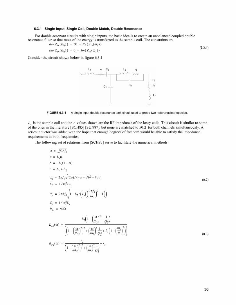
6.3.1 Single-Input, Single Coil, Double Match, Double Resonance
For double-resonant circuits with single inputs, the basic idea is to create an unbalanced coupled double resonance filter so that most of the energy is transferred to the sample coil. The constraints are
(6.3.1)
Consider the circuit shown below in figure 6.3.1
is the sample coil and the values shown are the RF impedance of the lossy coils. This circuit is similar to some of the ones in the literature [SCH85] [SUN87], but none are matched to 50 for both channels simultaneously. A series inductor was added with the hope that enough degrees of freedom would be able to satisfy the impedance requirements at both frequencies.
The following set of relations from [SCH85] serve to facilitate the numerical methods:
(0.2)
(0.3)
FIGURE 6.3.1 A single input double resonance tank circuit used to probe two heteronuclear species.
Re Zin ω( ) Re Zin ω( )
Im Zin ω( ) Im Zin ω( )
Ls
Cs
C1
rs
L1 r1
C2
L2 r2
C3
Ls rΩ
α f f⁄
a Lsα
b Ls α( )
c Ls L
ωt πf a( ) b b ac( )⁄
C ωtL⁄
ωs πkf L Ls
πfωt
-----------
⁄
Cs ωsLs⁄
Rin Ω
Leq ω( )
L ωω
------
Q
-------
ωω
------
ωω
------
Q
------- Ls ωs
ω------
-----------------------------------------------------------------------------------------------------------
Req ω( )r
ωωt-----
ω
ωt-----
Q
-------
----------------------------------------------------------- rs
56

For the reduced circuit shown in the figure below.
The constraint equations to solve for are
(0.5)
for
This numerical solution was found with Mathematica 3.0. A plot of the calculated parameter is shown below. This plot shows that at both widely separated frequencies, the probes are matched to 50 , with the reflected energy at least 40 dB down at each resonant frequency. In theory, this probe satisfies all the requirements – a single input, double resonance, double-matched probe at two widely separated frequencies.
Figure 0.4 Simplified schematic for the single input, double resonance probe.
FIGURE 6.3.2 for a double resonance probe, showing good matching at both frequencies. The effects of finite inductor quality factor has been included. Parameters used: =10 MHz, =40 MHz, =500 nH,
=1.8 H, =2 , =5 . All other parameters were found using the methods outlined above: =41.2 pF, =332 pF, =58.5 pF, =97.1 pF, =328 nH.
Leq(ω)
C1
Req(ω)
L1 r1
C2
C C k, ,( )
Req ωi( )
ωiLeq ωi( )C( ) ωiReq ωi( )C( )
------------------------------------------------------------------------------------------------ r Ω
ωiLeq ωi( ) ωiLeq ωi( )C( ) ωiReq
ωi( )C
ωiLeq ωi( )C( ) ωiReq ωi( )C( )
---------------------------------------------------------------------------------------------------------------------
ωiC
------------ ωiL
ωi πf πf,
SΩ
0 0.5 1 1.5 2 2.5 3 3.5 4 4.5 5x 10⁷
-80
-70
-60
-50
-40
-30
-20
-10
0
Frequency, (Hz)
|S11|
Sf f L
L µ r Ω rs ΩC Cs C C L
57
7.
Magnet Design
7.1 Homogeneity
For high resolution NMR and quantum computing, it is important for the effective spin-spin coherence time to be as long as possible. That is, for , from equation 2.5.2, ignoring contributions,
(7.1.1)
is , so for protons as the worst case scenario, since they have the highest gyromagnetic ratio, . Empirical evidence suggests that homogeneity is required for the experimental error to be negligible com-pared to natural decoherence. Empirical evidence has also shown that manufacturing tolerances of machined parts and surfaces leads to homogeneity over about a NMR sample tube of 0.5 mm in diameter. The remaining 3 orders of magnitude in homogeneity is obtained by a process known as shimming. A number of current-carrying spherical harmonic, orthogonal coils cause local perturbations of the static magnetic field to cancel out high spatial frequency magnetic flux density components. Consult [CHM90] for an excellent review.
The design goal for the remainder of this chapter will be to design magnets that have 1 ppM homogeneity over a 0.5 cm diameter spherical volume. Permanent magnets are the only static field magnet technology that would con-ceivably be suitable to simple, table-top application. The problem with typical permanent magnet design is flux return: traditional H and C-loop designs need hundreds of kilograms of steel/iron to construct a suitable magnetic cir-cuit. This chapter will present theoretical models of loopless or yokeless permanent magnets and conclude with finite element analysis to demonstrate success of the design criterion.
7.2 Maxwell’s Equations
Maxwell’s static equations are:
(7.2.1)
and (7.2.2)
where is the current density in a material, equal to zero for all further problems. The magnetic flux density is related to the magnetic field and magnetic magnetization by:
(7.2.3)
where
and , the remanent magnetization of the magnetic material. The field dependent magnetization can vary either linearly or non-linearly.
Figure 7.2.1 illustrates the J-H and B-H curves in the third quadrant for various modern hard magnetic materials. The B-H curve for neodymium-iron-boron is very linear. It is characteristic of a very good type II permanent magnet. The magnetization is fully saturated well past the coercivity, in the negative H direction. For other materials such as Alnico and ferrites, this approximation is not valid as the magnetization drops off very quickly after . In the region of interest, one can model the properties of materials such as neodymium-iron-boron (Nd-Fe-B) as linear, greatly simplifying further analysis:
(7.2.4)
T T→ T
T
------
T----- γ∆B
T s( ) γ∆B 4
5( )
6( )
∇ B× j
∇ B⋅
j
B µH J
J J Jm H( )
J Br
H Hc
Jm µχmH
58

is the susceptibility of the material. For a material such as Nd-Fe-B, the material is sufficiently magnetized in the entire region of interest of the B-H curve that . From 7.2.3 equation 7.2.4 can be re-written as:
(7.2.5)
where . (7.2.6)
Since these problems do not have any current densities, one can express equation 7.2.1 as:
(7.2.7)
where is the magnetic scalar potential. Combining this result with equations 7.2.2 and 7.2.5, one obtains Poisson’s equation:
(7.2.8)
In a region with no magnetization or if the magnetization is solenoidal , we get Laplace’s equation:
(7.2.9)
The last properties required for analysis are the boundary conditions on and in the absence of electric currents:
(7.2.10)
(7.2.11)
7.3 Halbach cylinders, spheres
We undertake a full theoretical description of a class of yokeless magnet designs that yield perfectly homoge-neous field solutions. It is difficult to obtain insight into the phenomena without the mathematical rigor that follows.
FIGURE 7.2.1 J-H and B-H curves for three permanent magnetic materials. The hyperbolic curves represent the energy density values for each material [ABE94].
χmχm ≈
B µrH J
µr µ χm( ) ≈
H Φ∇
Φ
∇Φ
µr-----∇ J⋅
∇ J⋅
∇Φ
B H
B B( ) n⋅
H H( ) n×
59
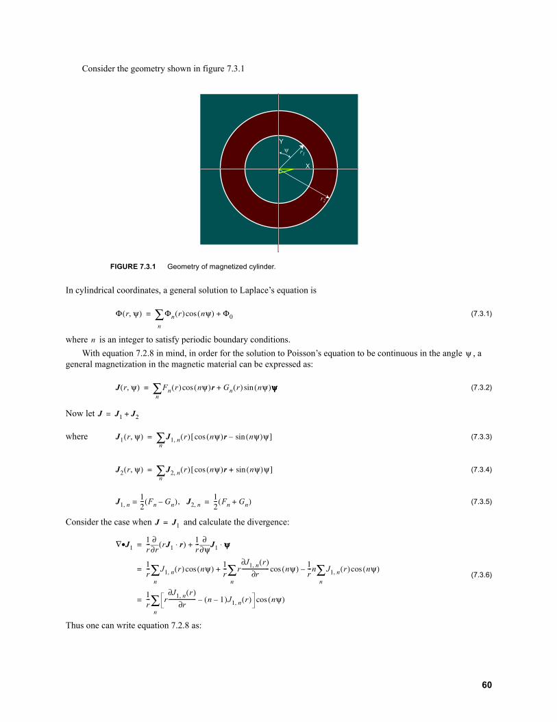
Consider the geometry shown in figure 7.3.1
In cylindrical coordinates, a general solution to Laplace’s equation is
(7.3.1)
where is an integer to satisfy periodic boundary conditions.
With equation 7.2.8 in mind, in order for the solution to Poisson’s equation to be continuous in the angle , a general magnetization in the magnetic material can be expressed as:
(7.3.2)
Now let
where (7.3.3)
(7.3.4)
(7.3.5)
Consider the case when and calculate the divergence:
(7.3.6)
Thus one can write equation 7.2.8 as:
FIGURE 7.3.1 Geometry of magnetized cylinder.
X
Yy r1
r2
Φ r ψ,( ) Φn r( ) nψ( )
n
∑ Φ
n
ψ
J r ψ,( ) Fn r( ) nψ( )r Gn r( ) nψ( ) ψψψψn∑
J J J
J r ψ,( ) J n, r( ) nψ( ) r nψ( ) ψ[ ]n∑
J r ψ,( ) J n, r( ) nψ( )r nψ( ) ψ[ ]n∑
J n,
--- Fn Gn( ) 7J n,
--- Fn Gn( )
J J
J∇•
r---
r∂∂
rJ r⋅( )
r---
ψ∂∂J ψψψψ⋅
r--- J n, r( ) nψ( )
n
∑
r--- r
J n, r( )∂r∂
-------------------- nψ( )
n
∑
r---n J n, r( ) nψ( )
n
∑
r--- r
J n,∂ r( )r∂
-------------------- n ( )J n, r( ) nψ( )
n
∑
60

(7.3.7)
where (7.3.8)
This was shown in [ABE94]. Writing , posit a solution of as . Solving equation 7.3.7 gives , and therefore
(7.3.9)
in the magnetic material. Since must remain finite over all space, the following conditions are imposed for the scalar potential:
(7.3.10)
Applying the boundary condition from equation 7.2.11, since taking the tangential component of the gradient of is simply a trivial change of sign ( for all terms), one can satisfy this constraint by mak-ing continuous. For the normal component of the flux density, by virtue of equations 7.2.5 and 7.2.7
(7.3.11)
where (7.3.12)
From equation 7.3.8, the above can be simplified to finally yield
(7.3.13)
Using these results gives a system of four equations with four unknown constants:
(7.3.14)
The solution of the above system of equations is
(7.3.15)
(7.3.16)
rr∂
∂r
r∂∂ Φ n, 8n( ) n Φ n, 8n( )
r∂∂
rn8n( )
µ
------rnJ n,
Φ n, 8n ∆ n, ∆ n, rα
α ±n
Φ n, 8n Cn , , rn Cn , , r n
Φ n,
Φ n,
Cn , rn
Cn , r n
r r<( )
r r>( )
Φ n,∂ Ψ∂⁄ nΨ( ) n nΨ( )
Φ n, r( )
Br r Ψ,( ) Br n, , r( ) nΨ( )n∑
Br n, , µ
Φ∂r∂
------- J n,
µ
8n∂r∂
--------- nCn , , rn nCn , , r n J n,µ
---------
Br n, , µ
nr--- Cn , , rn Cn , , r n 8n[ ]
Cn , Cn , , Cn , , rn
Cn , Cn , , Cn , , rn
Cn , , Cn , , rn Cn , r
n
Cn , , Cn , , rn Cn , r
n
8n r( )rn
8n r( )rn
8n r( )rn
8 n r( )rn
Cn , Cn , ,
Cn , , 8 n r( )rn
Cn , 8n r( )rn 8n r( )r
n
Φ n, r( )
r r<( )
µrn----------- rnJ n, rd
r
r
∫ r r r< <( )
µrn----------- rnJ n, rd
r
r
∫ r r>( )
61
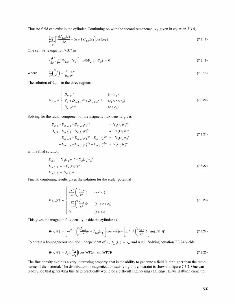
Thus no field can exist in the cylinder. Continuing on with the second remanence, given in equation 7.3.4,
(7.3.17)
One can write equation 7.3.7 as
(7.3.18)
where (7.3.19)
The solution of in the three regions is
(7.3.20)
Solving for the radial component of the magnetic flux density gives,
(7.3.21)
with a final solution
(7.3.22)
Finally, combining results gives the solution for the scalar potential
(7.3.23)
This gives the magnetic flux density inside the cylinder as
(7.3.24)
To obtain a homogeneous solution, independent of , and n = 1. Solving equation 7.3.24 yields
(7.3.25)
The flux density exhibits a very interesting property, that is the ability to generate a field in air higher than the rema-nence of the material. The distribution of magnetization satisfying this constraint is shown in figure 7.3.2. One can readily see that generating this field practically would be a difficult engineering challenge. Klaus Halbach came up
J
r--- r
J n,∂ r( )r∂
-------------------- n ( )J n, r( ) nψ( )
n
∑
rr∂
∂r
r∂∂ Φ n, 9n( ) n Φ n, 9n( )
r∂∂ 9n
rn------
µ
------J n,
rn---------
Φ n,
Φ n,
Dn , rn r r<( )
9n Dn , , rn Dn , , r n r r r< <( )
Dn , r n r r<( )
Dn , Dn , , Dn , , rn
Dn , Dn , , Dn , , rn
Dn , , Dn , , rn Dn , r
n
Dn , , Dn , , rn Dn , r
n
9n r( )rn
9n r( ) rn
9n r( ) rn
9n r( )rn
Dn , 9n r( )rn 9n r( )r
n
Dn , , 9n r( )rn
Dn , , Dn ,
Φ n, r( )
rn
µ
------J n,
rn--------- rd
r
r
∫ r r<( )
rn
µ
------J n,
rn--------- rd
r
r
∫ r r r< <( )
r r>( )
B r Ψ,( ) nrn J n,
rn--------- rd
r
r
∫ J n, r( ) nΨ( ) r nrn J n,
rn--------- rd
r
r
∫ nΨ( ) ΨΨΨΨ
r J n, r( ) J
B r Ψ,( ) Jrr----
nΨ( ) r nΨ( ) ΨΨΨΨ[ ]
62
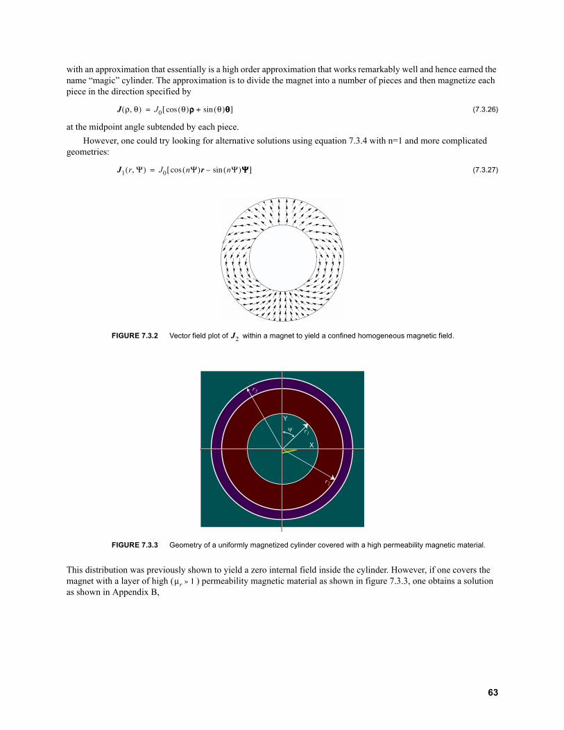
with an approximation that essentially is a high order approximation that works remarkably well and hence earned the name “magic” cylinder. The approximation is to divide the magnet into a number of pieces and then magnetize each piece in the direction specified by
(7.3.26)
at the midpoint angle subtended by each piece.
However, one could try looking for alternative solutions using equation 7.3.4 with n=1 and more complicated geometries:
(7.3.27)
This distribution was previously shown to yield a zero internal field inside the cylinder. However, if one covers the magnet with a layer of high ( ) permeability magnetic material as shown in figure 7.3.3, one obtains a solution as shown in Appendix B,
FIGURE 7.3.2 Vector field plot of within a magnet to yield a confined homogeneous magnetic field.
FIGURE 7.3.3 Geometry of a uniformly magnetized cylinder covered with a high permeability magnetic material.
J ρ θ,( ) J θ( ) ρρρρ θ( )θθθθ[ ]
J r Ψ,( ) J nΨ( ) r nΨ( ) ΨΨΨΨ[ ]
J
X
Y
y r1
r2
r3
µr :
63
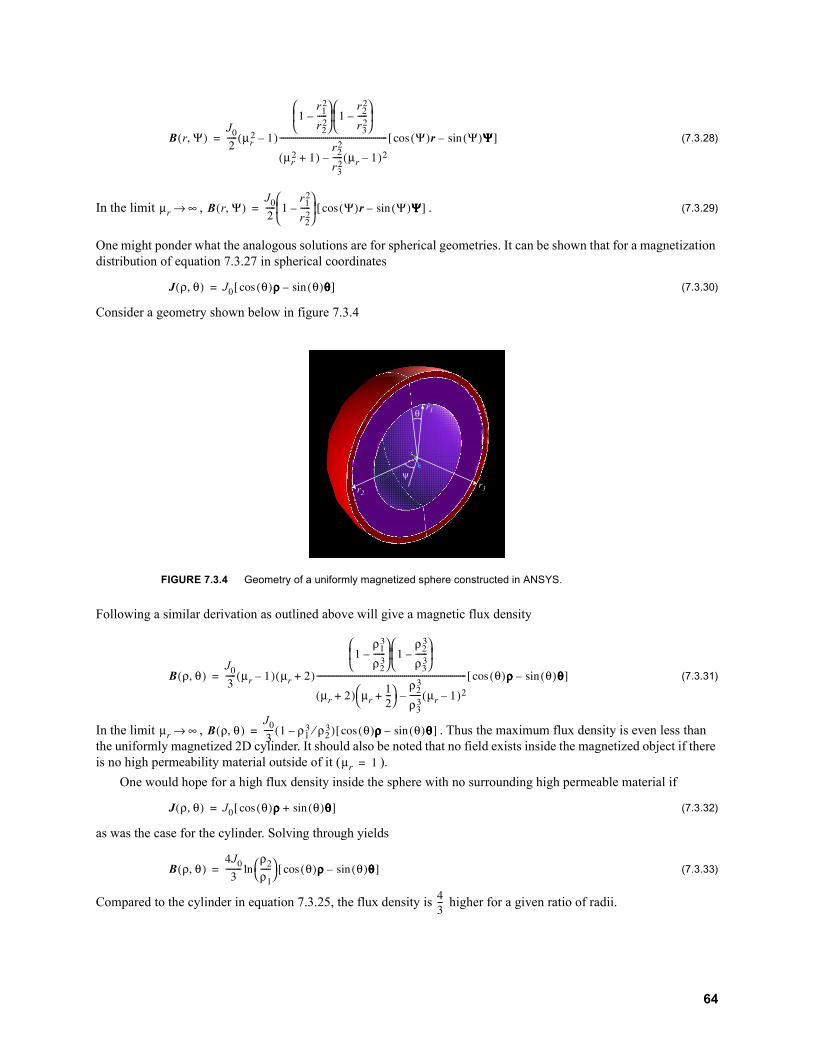
(7.3.28)
In the limit , . (7.3.29)
One might ponder what the analogous solutions are for spherical geometries. It can be shown that for a magnetization distribution of equation 7.3.27 in spherical coordinates
(7.3.30)
Consider a geometry shown below in figure 7.3.4
Following a similar derivation as outlined above will give a magnetic flux density
(7.3.31)
In the limit , . Thus the maximum flux density is even less than the uniformly magnetized 2D cylinder. It should also be noted that no field exists inside the magnetized object if there is no high permeability material outside of it ( ).
One would hope for a high flux density inside the sphere with no surrounding high permeable material if
(7.3.32)
as was the case for the cylinder. Solving through yields
(7.3.33)
Compared to the cylinder in equation 7.3.25, the flux density is higher for a given ratio of radii.
FIGURE 7.3.4 Geometry of a uniformly magnetized sphere constructed in ANSYS.
B r Ψ,( )J----- µr
( )
r
r
-----
r
r
-----
µr ( )
r
r
----- µr ( )
------------------------------------------------------ Ψ( ) r Ψ( ) ΨΨΨΨ[ ]
µr ∞→ B r Ψ,( )J-----
r
r
-----
Ψ( ) r Ψ( ) ΨΨΨΨ[ ]
J ρ θ,( ) J θ( ) ρρρρ θ( ) θθθθ[ ]
q
y
r1
r3r2
B ρ θ,( )J----- µr ( ) µr ( )
ρ
ρ------
ρ
ρ------
µr ( ) µr
---
ρ
ρ------ µr ( )
--------------------------------------------------------------------------- θ( )ρρρρ θ( )θθθθ[ ]
µr ∞→ B ρ θ,( )J----- ρ ρ⁄( ) θ( )ρρρρ θ( )θθθθ[ ]
µr
J ρ θ,( ) J θ( ) ρρρρ θ( )θθθθ[ ]
B ρ θ,( )J
--------ρρ-----
θ( )ρρρρ θ( )θθθθ[ ]
---
64

7.4 Manufacturing Tolerance Issues
In the finite element calculations that follow, manufacturing tolerances and magnets with non-ideal magnetiza-tion could pose dire consequences for a good design. Simply using many magnets to construct a larger magnet with no high permeability material can cause errors to add up quickly. There are two workarounds– the first is to construct the magnet out of many tiny magnets. With enough magnets, the statistics of the distribution of errors for the ensem-ble of magnets should average out high spatial frequencies in the magnetic field. The second method is more practical and simply required judicious placement of high permeability materials. From Laplace’s equation in equation 7.2.8, taking the Fourier transform in space yields
(7.4.1)
where is the spatial Fourier transform of . The frequency component will be attenuated by a factor of . If is high, true before the knee of ferrous magnetic materials, the high permeability enhances the filter-ing of Laplace’s equation by a factor over using permanent magnet materials alone. Subsequent work after these preliminary calculations will need to include this observation.
7.5 FEA
In the sections that follow, finite element calculations of the magnet models described in section 7.3 are con-structed. As was mentioned in the introductory paragraph, the best one can hope for in the magnet design is 1 ppM homogeneity over the sample, a 0.5 cm diameter spherical volume. To test these ideas, the finite element package, ANSYS 5.3 was used. It is a standard magnetostatic analysis package that is used widely in industry for modelling a range of physical objects: hard disk drives, cars, bridges and much more. It has proven itself in industry to be an accu-rate, reliable tool to analyze a system in conjunction with physical fabrication. The ANSYS package is a rare one that actually specifies the numerical stability of their system, allowing error bounds to be put on output. Documentation specifies that realistic precision of results should be on the order of 1 ppm due to numerical instability [ANS98], so within numerical precision the design requirement can be met. To test convergence, a variety of meshes for each model were constructed and the meshes documented here are those that required the least number of elements to sys-tematically obtain precise and accurate results compared to higher order meshes. The analysis that follows is a unique contribution.
7.5.1 Uniformly Magnetized cylinder with high permeability material cover
The geometry considered for this problem was shown in figure 7.3.3, and the 2-D mesh used in modeling is shown below in figure 7.5.1
The material data for the neodymium-iron boron magnet was taken from figure 7.2.1, with a coercivity of 944,000 A/m and a remanence of 1.23 T. The surrounding material was a linear material with permeability =100,000. The inner radius of the magnet was = 4 cm and the outer radius was = 6.5 cm. The magnet was magnetized in the
FIGURE 7.5.1 Part of the Finite element model constructed in ANSYS 5.3. The line shows where path plots of Bx and By.
Φ k( ) F k( )k k⋅( )µ
-------------------
F k( ) ∇ J⋅ F k( )dkk k⋅⋅⋅⋅( )µ µ
µr
µrr r
65

positive y direction. The radius of the high permeability magnetic material was = 7 cm. A flux plot for the solution is shown in figure 7.5.2.
Plotting over a 6 cm diameter in figure 7.5.3 shows the homogeneity of the field is excellent: far exceeding the specification required (actually on the order of one hundred parts per trillion). The expected flux density from equation 7.3.28 with a remanence of 1.23 T is = 0.3820 T. With the FEA result of 0.3826 T, the analysis is accu-rate.
7.5.2 Uniformly Magnetized, Non-linear Material Cover
Two areas of improvement over this design from section 7.5.1 are: (1) Use a real non-linear material for the high permeability cover to reflect realistic implementation and (2) Use a magnetization distribution to obtain flux densities higher than the remanence. To address the first issue the linear permeability was replaced with a real material, m3 grade steel, with a B-H curve shown in figure7.5.4. Since the material at high fields becomes saturated ( ), one would like the material to stay in the linear portion of the B-H curve: before the knee. Since the saturation field is very low, the highly permeable material must be thicker than that used before. This will make a table-top magnet larger than desired, but still relatively small. The radius of the high permeability was thus changed to = 9 cm. The flux line plot is shown below as well as the data in figures7.5.5 and 7.5.6 respectively. The homogeneity from the plots again exceeds the design requirement, about 100 parts per billion. Also, a slightly higher flux density is obtained than the previous case due to a larger effective . The use of non-linear material covers is a unique contri-bution.
FIGURE 7.5.2 Flux line plot for geometry with linear high permeability material.
r
By x( )
By
µr ≅
rBy x( )
r
66

FIGURE 7.5.3 Plot of and along y=0 line for a diameter of 6 cm. The homogeneity is 100 parts per trillion.
FIGURE 7.5.4 B-H curve for m3 steel used for high permeability cover.
FIGURE 7.5.5 Flux line plot for geometry with non-linear high permeability material.
Bx x( ) By x( )
67

7.5.3 Non-uniformly magnetized cylinder to obtain a high internal field
Recall from section 7.3, a continuous magnetization distribution created a flux density inside the cylinder greater than the remanence of the material. A Halbach distribution is illustrated in the ANSYS mesh constructed for a 12-piece geometry in figure 7.5.7. The orientation of the vector in each segment is at an angle
(7.5.1)
The geometry chosen was = 2 cm and = 6.75 cm. The flux line plot is shown in figure 7.5.8, and the flux density plots along a 0.6 cm contour are shown in figure 7.5.9. The homogeneity does not exist over as large a volume as the homogeneously magnetized cases, but still exceeds the design specifications. In addition, a much higher flux density within a smaller total field has been achieved. The flux density value of 1.513 T (the expected value is 1.410 T) is much higher than would be obtained from other methods. Scaling this to an sphere, the interior flux density should be 2.017 T.
FIGURE 7.5.6 Plot of and along y=0 line for a diameter of 3.5 cm for the m3 steel cover. The homogeneity is 100 parts per billion.
FIGURE 7.5.7 Mesh used for the “magic” cylinder and the magnetization orientation of each piece with respect to , the mean angle across a piece.
Bx x( ) By x( )
θiπi----- i …
r r
θi
68

FIGURE 7.5.8 Flux line plot for the magic cylinder.
FIGURE 7.5.9 Flux density plots of and along y=0 line for a diameter of 0.67 cm. The homogeneity is 100 parts per billion, exceeding the specification.
Bx x( ) By x( )
69

8.
Readout Techniques, Quantum Algorithms and Error-Correction
In this chapter, we discuss a number of important programming techniques for quantum computing, some spe-cific to NMR quantum computing. The chapter starts with the technique called state tomography, a technique to mea-sure all elements of the density matrix in NMR even though only the diagonal is observable. Following are two very important quantum algorithms that perform non trivial computations in less steps than can be obtained classically. The chapter ends with a discussion of quantum error correction, paramount to ensuring robustness of future quantum computers in the presence of noise.
8.1 State Tomography
To perform readout, it is important to be able to measure specific terms of the density operator. Since only terms which correspond to coherences can be observed, one must apply pulses to observe these terms. For example, for a two qubit system, the terms in the density matrix are
From figure 8.1.1, the system starts off in equilibrium ( =0) coherences. A single pulse to a single spin allows obser-vation of coherences representing in-phase terms like and antiphase -coupling terms like . Apply-ing pulses to both spins creates coherences, broken up into double quantum ( ) and zero quantum ( ) transitions. By applying a 0,1, or 2 pulse experiment, collecting the FID and Fourier transforming the data, measuring the real and imaginary components of the area of up to four peaks gives up to 4 complex numbers. The density matrix contains 16 complex numbers, and by making the following 9 experiments, one can measure all the terms in the density matrix using a least squares procedure: , where is the iden-tity, , and [CHU98b]. In general, for qubits, one needs to perform experiments to per-form state tomography, with up to peaks per experiment.
FIGURE 8.1.1 The different orders of coherence in the density matrix. The main diagonal terms represent classical probabilities (q=0), while the off diagonal terms represent single quantum coherences (q=0), double and zero quantum coherences (q=2).
p ±
P
P
P
P
|00⟩
|00⟩
|01⟩ |10⟩ |11⟩
|01⟩
|10⟩
|11⟩
|00⟩
|01⟩
|10⟩
|11⟩
ZQAB
ZQAB
2QAB
2QAB
1QA
1QB
1QB
1QB
1QB
|AB⟩
1QA
1QA
1QA
qq Ilx J IkxIlz
q | ⟩ | ⟩→| ⟩ | ⟩→
II IX XI IY YI XY YX XX YY, , , , , , , , IX R π ⁄( ) Y R π ⁄( ) N N
N
70
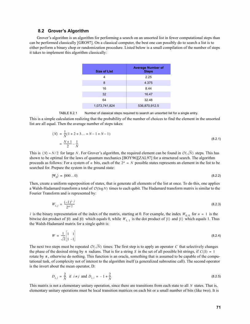
8.2 Grover’s Algorithm
Grover’s algorithm is an algorithm for performing a search on an unsorted list in fewer computational steps than can be performed classically [GRO97]. On a classical computer, the best one can possibly do to search a list is to either perform a binary chop or randomization procedure. Listed below is a small compilation of the number of steps it takes to implement this algorithm classically:
This is a simple calculation realizing that the probability of the number of choices to find the element in the unsorted list are all equal. Then the average number of steps takes:
(8.2.1)
This is for large . For Grover’s algorithm, the required element can be found in steps. This has shown to be optimal for the laws of quantum mechanics [BOY96][ZAL97] for a structured search. The algorithm proceeds as follows: For a system of bits, each of the possible states represents an element in the list to be searched for. Prepare the system in the ground state:
(8.2.2)
Then, create a uniform superposition of states, that is generate all elements of the list at once. To do this, one applies a Walsh-Hadamard transform a total of times to each qubit. The Hadamard transform matrix is similar to the Fourier Transform and is represented by:
(8.2.3)
is the binary representation of the index of the matrix, starting at 0. For example, the index for is the bitwise dot product of and which equals 0, while is the dot product of and which equals 1. Thus the Walsh-Hadamard matrix for a single qubit is:
(8.2.4)
The next two steps must be repeated times: The first step is to apply an operator that selectively changes the phase of the desired string by radians. That is for a string in the set of all possible bit strings, if rotate by , otherwise do nothing. This function is an oracle, something that is assumed to be capable of the compu-tational task, of complexity not of interest to the algorithm itself (a generalized subroutine call). The second operator is the invert about the mean operator, D:
and (8.2.5)
This matrix is not a elementary unitary operation, since there are transitions from each state to all states. That is, elementary unitary operations must be local transition matrices on each bit or a small number of bits (like two). It is
Size of ListAverage Number of
Steps
4 2.25
8 4.375
16 8.44
32 16.47
64 32.48
1,073,741,824 536,870,912.5
TABLE 8.2.1 Number of classical steps required to search an unsorted list for a single entry.
N⟨ ⟩
N---- … N N ( )
N
-------------
N----
N⟨ ⟩ N ⁄≈ N N( )
n n N
Ψ| ⟩ …| ⟩
N( )
Wi j,( )i j⋅
n /-----------------
i W , n
| ⟩ | ⟩ W , | ⟩ | ⟩
W
-------
N( ) Cπ S C S( )
π
Di j,
N---- 3i j≠ Di i,
N----
N
71

shown by Grover that the matrix can be decomposed into the elementary unitary operations where is the Walsh-Hadamard transform matrix from equation 8.2.3 and is a phase rotation matrix specified by:
(8.2.6)
Boyer et al have obtained an explicit closed form solution for the number of iterations to obtain with near unity prob-ability [BOY96]. The basic argument is to represent the ket as:
(8.2.7)
After the oracle, the state is
(8.2.8)
The mean of this is , so after the invert about the mean operation, one has
(8.2.9)
This establishes a coupled recursion relationship
(8.2.10)
Letting , the explicit solution is
(8.2.11)
, the desired solution equals 1 when . The number of steps required is thus . For large N, and the number of steps is thus . It has been shown that the probability of failure is no worse than if the algorithm is repeated times. A table of the number of steps required is shown in table
This algorithm has already been implemented on a real quantum computer: Isaac Chuang et al. have imple-mented Grover’s algorithm on labelled chloroform on a commercial NMR spectrometer [CHU98a]. The and
serve as the two qubit molecule. The authors hand compiled the algorithm to a simple pulse sequence. For exam-
Size of ListAverage Number of
Steps
4 1
8 1.67
16 2.61
32 3.92
64 5.77
1,073,741,824 25,375
TABLE 8.2.2 Average number of steps required to search an unsorted list using Grover’s algorithm.
D D WRW WR
Rii /i
Rij 3i j≠
R
Ψ| ⟩ k io| ⟩ l ii| ⟩ii i≠
N
∑
Ψ| ⟩ k io| ⟩ l ii| ⟩ii i≠
N
∑
k N ( )l
N---------------------------------
Ψ| ⟩ N
N-------------k
N
N-------------l
io| ⟩ N
N-------------l
N----k
ii| ⟩ii i≠
N
∑
kj
N
N-------------kj
N
N-------------lj
lj
N
N-------------lj
N----kj
θ
N----
kj j ( )θ( )
lj
N ----------------- j ( )θ( )
kj j ( )θ π ⁄ mπ θ
θ---------------
θ θ≅ mπ--- N
N⁄ π N ⁄
C
C
H
72
ple, the Walsh-Hadamard transform can be implemented as: where and pulses are applied from right to left [CHU98a]. is a rotation about the axis and is a rota-tion about the - axis. Since the whole algorithm is about 20-30 pulses for 2 qubits, this algorithm is a good starting point for demonstration of a working quantum computer. The first milestone for this project will be to demonstrate Grover’s algorithm working on our table-top apparatus.
8.3 Shor’s Algorithm
Shor’s algorithm is the prodigy of the quantum computing community – it is the standard by which all algorithms are compared and the ultimate goal for hardware development. It is a marvel that breaks the divide between classical algorithms and quantum algorithms, because, as was stated in section 1.2, it demonstrates a useful exponential speed-up over all known classical algorithms for the problem of prime factorization. This algorithm is an important demon-stration of finding the period of a function. Suppose a function is function with period such that = . If can be computed efficiently, and we know that . Classically, to find his periodicity involves
function evaluations. This is inefficient since the number of function evaluations is exponential in the infor-mation size of the input, .
The factorizing problem reduces to finding the periodicity of the function for a number coprime to N, chosen at random. For large N, a randomly chosen will work with probability greater than . To factor an odd number with period such that , compute the function gcd( , ). gcd( ) is the greatest common divisor that divides both and . A polynomial time algorithm for gcd( ) was solved by Euclid in 300 BC. Since = , the gcd( , ) will be a factor of unless is odd or if . The probability of success was shown by Shor to be was is the number of distinct odd prime factors of [SHO95].
The quantum algorithm requires qubits ( ), plus another for scratch space (optimizing this algorithm can require much more – in [BEC96], qubits are required). Two registers are labelled, and , both initially in the ground state. Next, one puts the first register into a uniform superposition of states
(8.3.1)
This can be implemented with a Hadamard transform (section 8.2) or a discrete Fourier transform to be shown later. The next step is to compute the function and store contents in register . After a single application, the system is in the state
(8.3.2)
Next, one makes a measurement on . If the value of the measured signal is , the -register collapses into the state and the remaining state is
(8.3.3)
where . The register remains in a superposition of states.
Next one needs to implement the quantum Fourier transform on the x register so that
(8.3.4)
Since this algorithm works on an exponentially large register, it is important than this is a polynomial time transfor-mation. An algorithm was found independently by Coppersmith [COP94] and Deutsch [EKE96]. Coppersmith also showed that exponential precision in the Fourier transform is not necessary for large , and an approximate one that
W HA HB⊗ H XY
X iπIx ⁄( ) $° x Y iπIy ⁄( ) $°y
f x( ) r f x( ) f x r( )f x( ) N ⁄ r N< <
N ⁄( )N
f x( ) ax,!' a N<a ⁄
N r ar,!N ar ⁄ ± N α β,α β α β,
ar ⁄ ( ) ar ⁄ ( ) ar ( ),!N ar ⁄ ± N N rar ⁄ ,!N k k
N
n n N n( )n x y
n ⁄----------- x| ⟩ | ⟩
x
n
∑
f x( ) ax,!N y
n ⁄----------- x| ⟩ ax,!N| ⟩
x
n
∑
f x( ) u yu| ⟩
M ⁄------------- du rj| ⟩ u| ⟩
j
M
∑
M n r⁄≅ x M
x| ⟩
n ⁄----------- πixk
n--------------
k| ⟩
k
n
∑→
n
73

avoids tiny phase factors can also implement this algorithm [COP94]. Up until now, the exact case has been dealt with. From here, the ideal case where will be discussed to illustrate the ideas. [SHO95] considers the exact case when does not divide exactly, but the essential ideas are the same. Since the Fourier transform of a pulse train is a scaled (amplitude and frequency) pulse train in the frequency domain, one is left with the following func-tion
(8.3.5)
where
(8.3.6)
If the state in the register is now measured, one will be a multiple of or . If and have no com-mon factors, make an irreducible fraction and obtain and . If they share common factors, the algorithm must be repeated. After approximately steps, the probability of success is arbitrarily close to unity [EKE96][STE97].
The number field sieve [SHO95], the best classical algorithm to date, takes steps. Shor’s factoring algorithm requires steps, exponentially faster. The smallest number that can be factored using Shor’s factoring algorithm is the number 15. This is out of the realm of current quantum computing technology using NMR, but through larger molecule design and sensitive electronics should be feasible in the coming years. This algorithm will be an important milestone for experimental quantum computing if a successful implementation can be made.
8.4 Quantum Error Correction
In any physical quantum computer, loss of quantum coherence will be inevitable – no system is perfectly isolated from a bath and no applied gate can be perfect. Classical computers face the same dilemma, but they overcome this problem by being insensitive to noise, and hence do not require error correction circuitry. Each gate in an integrated circuit is like a switch: small perturbations force the system back to its equilibrium position with a high degree of nonlinearity. To be able to do this requires amplification and dissipation. In quantum mechanics, the no cloning theo-rem prevents making copies of unknown quantum states [PER93], and since quantum mechanics is reversible, dissi-pation is not possible.
These ideas led many to believe that quantum error correction was not possible without repeated measurement, destroying all utility of quantum computing since superposition states and entanglement would be lost. Fortunately classical information theory provided an answer. Consider the [7,4,3] Hamming code:
A [n,k,d] Hamming code is a -bit vector encoding bits which corrects errors. The Hamming distance between two equal length vectors is obtained by performing binary addition of the two strings and counting the num-ber of 1s or the places where they differ. The Hamming code words all have a Hamming weight of , or 3 in this example. Consider the parity check matrix
Word Hamming code word
0000 0000000
0001 1010101
0010 0110011
0011 1100110
0100 0001111
0101 1011010
TABLE 8.4.1 Classical error correction. Here are the firs 6 of 16 elements of a [7,4,3] Hamming code to detect and correct single errors without finding any information about the input state.
M n r⁄
r n δδ
r------ k( ) k| ⟩
k∑
k( ) 3k,/ 3n r⁄ ;
x n r⁄ mλn
r--------- λ r
λ rr
c n( ) ⁄ n( ) ⁄( ) ( ) n( ) n( ) n( )
n k d ( ) ⁄
d
74
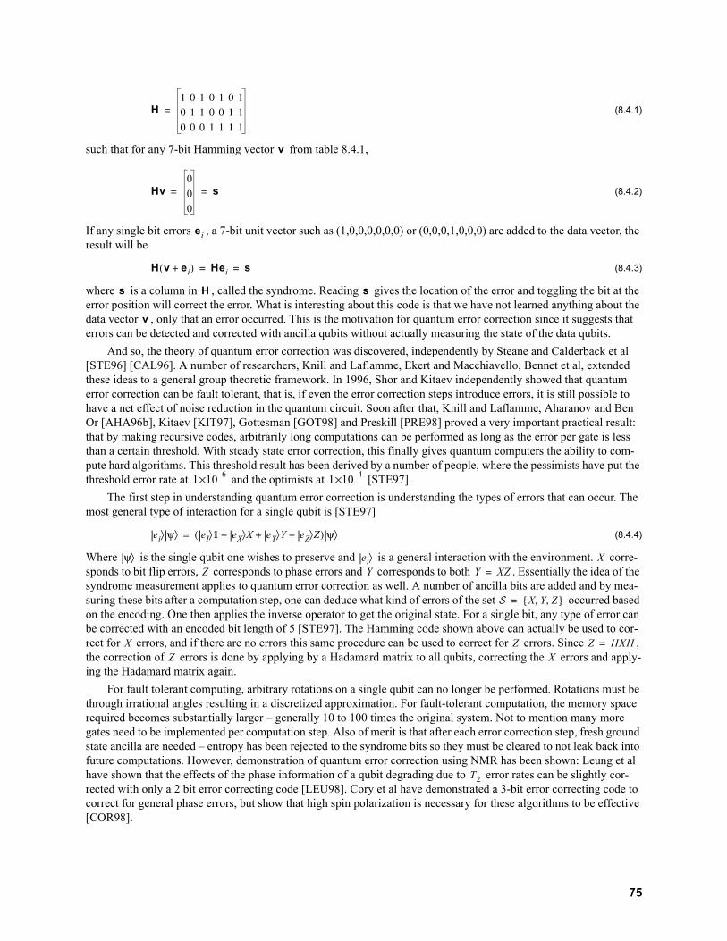
(8.4.1)
such that for any 7-bit Hamming vector from table 8.4.1,
(8.4.2)
If any single bit errors , a 7-bit unit vector such as (1,0,0,0,0,0,0) or (0,0,0,1,0,0,0) are added to the data vector, the result will be
(8.4.3)
where is a column in , called the syndrome. Reading gives the location of the error and toggling the bit at the error position will correct the error. What is interesting about this code is that we have not learned anything about the data vector , only that an error occurred. This is the motivation for quantum error correction since it suggests that errors can be detected and corrected with ancilla qubits without actually measuring the state of the data qubits.
And so, the theory of quantum error correction was discovered, independently by Steane and Calderback et al [STE96] [CAL96]. A number of researchers, Knill and Laflamme, Ekert and Macchiavello, Bennet et al, extended these ideas to a general group theoretic framework. In 1996, Shor and Kitaev independently showed that quantum error correction can be fault tolerant, that is, if even the error correction steps introduce errors, it is still possible to have a net effect of noise reduction in the quantum circuit. Soon after that, Knill and Laflamme, Aharanov and Ben Or [AHA96b], Kitaev [KIT97], Gottesman [GOT98] and Preskill [PRE98] proved a very important practical result: that by making recursive codes, arbitrarily long computations can be performed as long as the error per gate is less than a certain threshold. With steady state error correction, this finally gives quantum computers the ability to com-pute hard algorithms. This threshold result has been derived by a number of people, where the pessimists have put the threshold error rate at and the optimists at [STE97].
The first step in understanding quantum error correction is understanding the types of errors that can occur. The most general type of interaction for a single qubit is [STE97]
(8.4.4)
Where is the single qubit one wishes to preserve and is a general interaction with the environment. corre-sponds to bit flip errors, corresponds to phase errors and corresponds to both . Essentially the idea of the syndrome measurement applies to quantum error correction as well. A number of ancilla bits are added and by mea-suring these bits after a computation step, one can deduce what kind of errors of the set occurred based on the encoding. One then applies the inverse operator to get the original state. For a single bit, any type of error can be corrected with an encoded bit length of 5 [STE97]. The Hamming code shown above can actually be used to cor-rect for errors, and if there are no errors this same procedure can be used to correct for errors. Since , the correction of errors is done by applying by a Hadamard matrix to all qubits, correcting the errors and apply-ing the Hadamard matrix again.
For fault tolerant computing, arbitrary rotations on a single qubit can no longer be performed. Rotations must be through irrational angles resulting in a discretized approximation. For fault-tolerant computation, the memory space required becomes substantially larger – generally 10 to 100 times the original system. Not to mention many more gates need to be implemented per computation step. Also of merit is that after each error correction step, fresh ground state ancilla are needed – entropy has been rejected to the syndrome bits so they must be cleared to not leak back into future computations. However, demonstration of quantum error correction using NMR has been shown: Leung et al have shown that the effects of the phase information of a qubit degrading due to error rates can be slightly cor-rected with only a 2 bit error correcting code [LEU98]. Cory et al have demonstrated a 3-bit error correcting code to correct for general phase errors, but show that high spin polarization is necessary for these algorithms to be effective [COR98].
H
v
Hv
s
ei
H v ei( ) Hei s
s H s
v
×10
×10
ei| ⟩ ψ| ⟩ eI| ⟩ eX| ⟩X eY| ⟩Y eZ| ⟩Z ( ) ψ| ⟩
ψ| ⟩ ei| ⟩ XZ Y Y XZ
X Y Z, ,
X Z Z HXH
Z X
T
75

9.
SNR Calculations
9.1 Introduction
NMR is a wonderful experimental technique that has not met widespread application due to a limited intrinsic sensitivity. In NMR ensemble quantum computing at finite temperature, sensitivity becomes even more of an issue. As will be shown in chapter 12, without polarization enhancement of the nuclear magnetization, the sensitivity of the NMR signal drops exponentially as the number of qubits in the system grows. Therefore it is important to do noise calculations of any desired system to compare performance in terms of how many qubits can be accommodated with reasonable sensitivity. Noise calculations may also offer insight into system design optimizations that could yield more qubits. In the literature, the signal to noise ratio is expressed in terms of coupled variables which makes comparative calculations difficult [HOU76]. Also, standard calculations usually only consider fluctuation dissipation noise, leaving out other intrinsic noise sources such as equipartition noise and spin noise. This chapter is meant to contribute to this area by giving a method for performing signal to noise ratio calculations for arbitrary coil geome-tries and all noise contributions. This contribution is a consolidation of disparate results in the field. Coils were cho-sen for this analysis since at reasonable flux density strengths , no other measurement technique used thus far can obtain this sensitivity on macroscopic scales, as will be shown in this chapter.
9.2 Solenoid/Cavity Resonator (Nyquist and Equipartition Noise)
We state the standard formula for the signal-to-noise ratio in NMR and then will re-derive it more generally with respect to uncoupled variables to shed some more light on this complex issue. The signal to noise ratio [HOU76] after a pulse from an ideal solenoidal coil is given by:
(9.2.1)
is a factor indicating the homogeneity of the field from the receiving coil; is the fill fraction; is the nuclear magnetization, proportional to the applied magnetic field ; is the volume of the coil; is the noise fig-ure of the amplifier; is Boltzmann’s constant; and is the bandwidth of the receiver. This equation is correct in the signal term, but very difficult to draw conclusions from since many variables are coupled. is itself a function of
, volume and , from the standard result for solenoidal coils , where is the diameter of the coil in inches [HOU89]. This equation does not include all possible noise sources: equipartition and spin noise are neglected. This will be included later in this section, an original contribution.
Equation 9.2.1 can also be derived using the principle of reciprocity from [HOU89]. Equality of the two methods only holds for solenoidal coils, but this reciprocity principle is more powerful as it allows the possibility of other coil geometries. This principle is based on the idea that the induced signal from a finite volume of magnetization crucially must depend on its spatial displacement from the coil if the coil has finite extent and an inhomogeneous RF field. The signal from nuclear spins to be detected using the principle of reciprocity is from the principle of reciprocity,
(9.2.2)
is the field produced by the coil at a point per unit of current. This will yield Lenz’s Law if the field is inde-pendent of cartesian coordinates, only true for spheres, ellipses and infinitely long cylinders. We will approximate this integral by assuming is reasonably homogeneous over the sample and of the form . Let us assume:
( )
T( )
$
Ψrms KηMo µoQωoVc( ) FkBT∆f( )⁄ ⁄
K B η MoBo Vc F
kB ∆fQ
ωo K Q d f≈ d
vt∂
∂B M⋅( ) Vsd
S∫
B
B B B( )xy ωt( )
76

(9.2.3)
where and from Zeeman splitting, a paramagnetic system of spin ½ nuclei has a magneti-zation (for )
(9.2.4)
where is the number of spins per unit volume.
From the equipartition theorem, an inductor in series with a dissipative source such as a resistor has a mean value of its noise energy equal to . Thus the rms noise voltage produced across the inductor, of impedance is
(9.2.5)
From Nyquist’s theorem from the fluctuation dissipation theorem in thermodynamics, the voltage spectral density from a resistor is [SLE87]
(9.2.6)
In the high temperature limit this becomes
(9.2.7)
To obtain the rms voltage,
(9.2.8)
Thus the noise voltage over a bandwidth becomes
(9.2.9)
This is Nyquist’s famous result. Both voltage terms will be further downgraded by a factor of , the total noise figure of the receiver. The total SNR can be obtained as:
(9.2.10)
As from section 5.6, for a conductor of circumference , the resistance is where is the skin depth of the wire and is the total length of wire.The resistance calculation is only approximate for cylindrical conductors that do not interact with nearby conductors. Combining this into equation 9.2.10 yields:
(9.2.11)
Note that this can be turned in to equation 9.2.1 with an ideal solenoid and the appropriate substitutions. All things being equal for numerous coil geometries, and ignoring equipartition noise, the SNR is proportional to the following important quantities for numerous coil geometries:
(9.2.12)
From this equation, it becomes apparent that much higher signal to noise ratios can be obtained from surface coils rather than wound coils, since the circumference of the conductor will be that of the overall geometry rather than the wire itself. Consider an example of a solenoid of diameter and length . For the solenoid,
B M⋅( ) VsdS
∫ K B( )xy
M
M χB µ⁄ χ ω γ⁄ µ( )
!ω kBT4
Mo
Nγ!B
µokB
T---------------------
N
---L I⟨ ⟩
---kBT jωL
VL⟨ ⟩ Lω
kT
R
Sv ω( )
π---R!ω !ω
kBT------------
Sv ω( )
π---RkBT
Vs⟨ ⟩ Sv ω( ) ωd
∞
∞
∫
∆f
VR⟨ ⟩ RkBT∆f
F
Ψrms
πfγ!NK B( )
xyVs
F∆fR FπfL kBT( ) ⁄-----------------------------------------------------------------
p R lT pσδ( )⁄≈ δ πµfσ⁄
lT
Ψrms
π ⁄f ⁄
NKγ! B( )xy
Vs
kBT( ) ⁄------------------------------------------------------------- p
F lT∆f πfL( )----------------------------------------
⁄ σµ------
⁄
Ψrms K B( )xy
VsplT----
⁄∝
a a
77

(9.2.13)
The length can be approximated as . According to [TER43] the optimal radius of conductor is such that the spacing between conductors is . From this optimality constraint,
(9.2.14)
Combining this with equation 9.2.13, a final proportionality for the SNR for large is .
9.2.1 Spin Noise
Spin noise is the phenomenon of random fluctuations in the transverse components of magnetization. Physically, the source of this noise is spontaneous emission in equilibrium with an external circuit, in this case the coil. This may seem at first to be impossible. At and above optical frequencies, spontaneous emission of electric dipoles is easily detected in free space - magnetic dipole radiation is much less common. The reason is as was derived by Einstein, for magnetic dipoles, the spontaneous emission rate is proportional to [SLE87]. For 30 MHz RF energy radiated from a nuclear spin, the spontaneous emission rate is 28 orders of magnitude less than optical rates, the actual nuclear rate in free space being Hz. However, at wavelengths larger than or on the order of a cavity, it is possible to couple to cavity modes and via the enhanced through radiation damping achieve a larger rate [KLE81]. Sleator et al [SLE87] state the enhancement factor for a cavity mode coupling is where is the volume of the sample. For a of 1000 and a 1cm3 volume, the enhancement factor is approximately 1011. With approximately 1022 spins in this sample, the probability of observing this phenomena becomes increasingly likely and various groups have observed this noise with low-temperature DC SQUID amplifiers [SLE87] and in protons in water at room temperature [GUE89]. To derive the noise spectral density, we start by creating a source of dissipation for fluc-tuations to occur. Since we are ultimately interested in a rms voltage, this will be a resistor in series with the resonant tank circuit, , which has a voltage spectral density according to 9.2.6. To find out what this resistance is, we resort to the Bloch equations for the complex spin susceptibility [SLI96]
(9.2.15)
This susceptibility slightly changes the inductance of the coil so that the complex impedance is
(9.2.16)
where is the filling factor, the ratio of the sample to coil volume respectively. Combining the last two equa-tions gives a real resistance
(9.2.17)
Using the Bloch equations, Slichter shows for spin-spin relaxation ,
(9.2.18)
where is the Larmor frequency. has already been derived in equation 2.1.14. Combining equations 2.1.14, 5.7.18 and 9.2.18, the spectral density for all temperature is
(9.2.19)
This is very surprisingly independent of temperature (not true for spins other than [SLE87]). To get the rms voltage, integrating over all frequencies gives
(9.2.20)
One could also get this result from Faraday’s law and noting that the mean square magnetization is independent of temperature and is
B( )xy
µon
⁄
-----------
lT πan≈r
r n ( ) a
pπa
n ( )--------------------
n Ψrms Vs∝
νµ
#×10
QQc πνvs⁄ vs
Q
Rs
χ ω( ) χ' ω( ) iχ'' ω( )
Zin iωLt iωL πξχ ω( )[ ]
ξ vs vc⁄
Rs πξLωχ'' ω( )
T
χ'' ω( )Mz⟨ ⟩ γT
ωl ω( )T( )
-----------------------------------------------
ωl Mz⟨ ⟩
Sv ω( )ξ!ωγNLT ωl ω( )T
( )--------------------------------------------
---
Vs⟨ ⟩ πξ!ωγNL
78
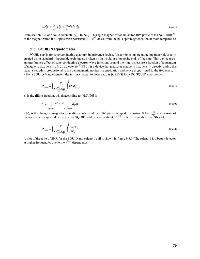
(9.2.21)
From section 2.2, one could calculate to be . This spin magnetization noise for 1022 particles is about of the magnetization if all spins were polarized, down from the bulk spin magnetization at room temperature.
9.3 SQUID Magnetometer
SQUID stands for superconducting quantum interference device. It is a ring of superconducting material, usually created using standard lithographic techniques, broken by an insulator at opposite ends of the ring. This device uses an interference effect of superconducting electron wave functions around the ring to measure a fraction of a quantum of magnetic flux density, . It is a device that measures magnetic flux density directly, and so the signal strength is proportional to the paramagnetic nuclear magnetization and hence proportional to the frequency,
.For a SQUID Magnetometer, the intrinsic signal to noise ratio is [GRE98] for a DC SQUID measurement,
(9.3.1)
is the filling fraction, which according to [HOU76] is
(9.3.2)
is the change in magnetization after a pulse, and for a pulse, is equal to equation 9.2.4. is a measure of the noise energy spectral density of the SQUID, and is usually about J/Hz. This yields a final SNR of:
(9.3.3)
A plot of the ratio of SNR for the SQUID and solenoid coil is shown in figure 9.3.1. The solenoid is a better detector at higher frequencies due to the dependence.
Mx⟨ ⟩ N
vs---- µx
⟨ ⟩ Nvs----γ! Ix
⟨ ⟩
Ix⟨ ⟩
---
×10
×10
h e⁄ $×10 Wb≅
f
Ψrms
ηVs
FεSQe( )∆fµo
-------------------------
---
∆Mo( )xy
η
η B
Vd
,
∫ B
Vd
∫⁄
∆Mo $ εSQ
e( )
Ψrms
ηVs
FεSQe( )∆fµo
-------------------------
---πNγ!fkBT
------------------
f ⁄
79
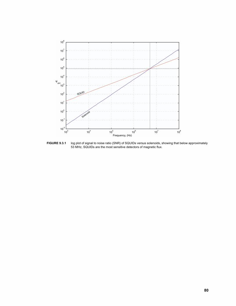
FIGURE 9.3.1 log plot of signal to noise ratio (SNR) of SQUIDs versus solenoids, showing that below approximately 53 MHz, SQUIDs are the most sensitive detectors of magnetic flux.
103
104
105
106
107
108
10-2
10-1
100
101
102
103
104
105
106
107
108
Frequency, (Hz)
Ψsnr
Solenoid
SQUID
80

10.
Hardware Design
10.1 Overall design methodology
The general pieces needed for a table top design are shown in figure 10.1.1. A magnet is required to create the Zeeman splitting for magnetic resonance. To implement gates, a coil is placed around the sample to couple magnetic energy into the system. A transmitter translates an IF signal to the Larmor frequency with a mixer and then amplifies the signal to the appropriate levels outlined in section 6.1. Having an IF frequency is important so that no components in the transmitter other than the transmit signal itself are generating power at the Larmor frequency. Otherwise signif-icant noise power will be generated that can couple into the receiver. In the simplest case, pulses are applied by gating a stable source oscillator, generating so called hard pulses. More complex instruments are able to generate arbitrary waveforms for more articulate types of spin control. The most common type of arbitrary waveform is called a soft pulse: gaussian or cosine modulated waveforms that manipulate specific spins within a homonuclear subspace. Soft pulses tend to be several milliseconds in length for protons, hundreds of microseconds for carbon nuclei. Usually, the same coil is used to detect the small NMR signal. Analog superheterodyne receivers are generally chosen based on the assumption that noise at different frequencies is uncorrelated. A high isolation switch is needed to protect the low noise receiver from 9-12 orders of magnitude larger signals. Finally a computer acquisition system samples the data, and basic signal processing techniques such as Fast Fourier Transforms and digital filtering are applied to simplify analysis.
10.1.1 Spectrometers
For current demonstrations of quantum algorithms using NMR, people have used heteronuclear and homonu-clear spin addressing, gradient fields and hundreds of pulses [CHU98a] [VAN99] [COR98], pushing the state of the art NMR spectrometers. To be useful, any proposed quantum computer based on NMR must have at least this func-tionality – a very versatile RF transmitter, receiver and signal processing system. For this project a complementary goal is to make a general set of electronic devices for interrogating spins at different levels of description (NMR quantum computing, chemical spectroscopy, medical imaging, tagging applications etc.). This second goal adds another constraint – cost. Many interesting applications of NMR are out of reach because the technology is far too expensive. Looking at the semiconductor industry and pace of progress, especially in wireless communications, one
FIGURE 10.1.1 A canonical NMR spectrometer schematic.
Bo
low noiseamplifier
mixer
computerRFOscillator
RFcoil
amplifiermixer
(magnetic field)
sample
81

can readily see that detecting extremely small signals (-110 dBm) for low cost ($3.00) is possible [MOT99]. Since this application is being developed for moderately low field permanent magnets, a software radio approach becomes very appealing. This approach offers versatility at very low cost. In this paradigm, the signal chain is kept digital as much as possible. Ideally, the Larmor frequency with waveform shaping could be generated directly from a fast A/D converter for the transmitter, and the IF frequency on the receiver could be sampled directly, filtered, decimated and digitally downconverted.
10.2 Commercial Spectrometers – Prior Art
The current state of the art spectrometers centers around a large cylindrically symmetric superconducting mag-net. Based on equation 9.2.11, magnets tend to be superconducting to maximize signal-to-noise ratio. These magnets routinely generate magnetic fields between 10-20 Tesla (T) and have masses between 120-12,000 kg [OXF99]. These magnets require both Nitrogen and Helium cooling. They have superconducting and room temperature shim coils to reach ppB magnetic field homogeneity over a 10 cm long by 10 mm diameter sample. Current spectrometers have a great deal of control, making them useful for a number of applications. The sample can be changed automatically, temperature can be adjusted within the magnet chamber and the sample can be spun, to help remove inhomogeneous broadening effects [CHM90]. Probes can address up to three heteronuclear species, cost up to $30,000 and represent 30 years of engineering refinement. For the RF electronics, a large rack of digital and analog electronics allow spin manipulation on all levels. On the transmitter side, arbitrary waveform generation can be provided. The transmitter frequency can be varied during an experiment, and gating resolution is on the order of 100 ns. On the receiver end, careful receiver design has brought the overall system noise to figure to dBm. Most of the signal chain is ana-log, including the quadrature detection and the sampled data is sampled at baseband with usually a 100 kHz, 12/16 bit A/D converter. Separate transmit and receive electronics exist for each heteronuclear species. A computer console is provided to allow full software control of all static and dynamic variables of the system. These machines cost on the order of a million dollars and occupy entire rooms. They are the mainframes of NMR but they do their job extremely well. Commercial spectrometers are the cutting edge research tool for experimental quantum computing.
On the table-top side, very little has been done. Only one company, Hitachi claims to have a machine capable of spectroscopy, but it is continuous wave (CW) based [HIT99b]. It is only capable of observing protons and the perma-nent magnet used weighs 550 pounds. All other systems have magnet homogeneity too low to perform any real spec-troscopy, essential for quantum computing [TEA99] [MRR99].
10.3 Preliminary NMR System
As a first pass to developing instrumentation, it was imperative to test the demands on instrumentation sensitiv-ity. Richard Fletcher, a graduate student, developed instrumentation to simply observe an NMR signal, based on an MIT Physics Laboratory, Junior Lab [KIR95]. The original hardware developed by Fletcher used analog timers for generating one or two pulses. This was a cumbersome approach to developing more complex pulse sequences. In addition, there was no means of storing receiver output – data was simply observed on an oscilloscope. In an effort to generalize pulse sequence generation, and allow for data acquisition, the original system was modified. A schematic of the transmitter and receiver developed by the author is shown below in figure 10.3.1 and a photograph of the first setup in figure 10.3.2. The contribution to this work is a dramatically simplified and generalizable pulse programmer and a data acquisition system, outlined below.
In this setup, a stable RF source generates the Larmor frequency directly and a pair of switches gate the RF to the probe. On the receive end, a number of low noise figure amplifiers receive the signal, mix down to DC from the trans-mitter source and then amplify the signal to digital sampling levels. The switches used were all the same: 0.5W GaAs, TTL input MiniCircuits switches [MIN99]. The heart of the pulse programmer was a low cost micro controller, a Microchip PIC16F84. It is a small 8-bit RISC processor capable of up to 2.5 MIPS [MIC99], allowing generation of pulses with sub microsecond resolution. A RS232 serial interface was created so that a user on a Personal Computer (PC) could dynamically change the pulse program for the spin system. Spin echoes were chosen as the pulse program for demonstration of simple spin control. For data acquisition, an integrator and A/D converter on a Microchip PIC16C76 were used. This only gave the area of a FID so this was replaced with a PC based, National Instruments 1 Msps, 12-bit A/D converter [NAT99]. The total system was capable of working from about 5 MHz up to 500 MHz, set by the receiver bandwidth. The probe was a very simple one: a capacitor matched LC resonator matched to
( )
Ω
82

as described in section 6.2. on a copper ground plane with no shielding. The capacitors chosen were simple Sprague Goodman GKG series ceramic trimming capacitors, chosen because they have no ferrous materials inside which would cause unnecessary inhomogeneity of the magnet. The coil was made simply by wrapping magnet wire around a small test tube filled with sample, as shown in figure 10.3.3.
FIGURE 10.3.1 Schematic of transmitter and receiver of preliminary NMR system.
FREQUENCYSOURCE
(HP stable analog oscillator)r.f Gate
Mini-Circuits
Scos(ωot)
PulseProgrammer,1 Msps Nat. Instr. D/A
A
PulseProgrammer
r.f. power amp, 4 W (Minicircuits)
AScos(ωot)
r.f GateMini-Circuits
To Rx
Low-noisePreamplifier
P.S.D.
Variable gainamplifier
FREQUENCYSOURCE (HP)
r.f Gate
Frequencyω l
PulseProgrammer
Variable gainL.P.F.
SIGNAL 1(X)
Mini-circuits SRS 560
TX
RX
83

10.3.1 Preliminary System Magnet
The initial magnet used is shown in figure 10.3.2. It is a C-style magnet, using a steel C-clamp for flux return, a pair of 2”x2”x1” neodymium iron boron (Nd-Fe-B) magnets, and mu-metal pole pieces to spread out the flux density across the gap. The mu-metal pole pieces were the most critical to the design to achieve parts per thousand homoge-neity. It became a necessity to have a smaller, more portable, more homogeneous magnet, so a 13 pound C-style mag-net was designed and built and is shown in figure10.3.4. This magnet had the flux return made from low carbon grade steel. The same Nd-Fe-B magnets were used and a new pair of mu-metal pole pieces were fashioned. This magnet achieved 100-1000 ppm homogeneity.
FIGURE 10.3.2 Photograph of the first NMR setup in this lab and the pulse programmer/data collector utilizing low cost microcontrollers. The magnet is in the upper left corner of the first picture.
FIGURE 10.3.3 The first probe: a capacitor matched LC resonator on a copper backplane. The sample is on the right wrapped in magnet wire.
84

.
10.4 Electromagnet
The preliminary system and permanent magnet was designed for simple spin manipulation, and with additional instrumentation could be made to implement any phase rotation about the Bloch sphere. The next major challenge was to try to demonstrate logic, a process that involves interaction between spins. Just to show that this instrumenta-tion was capable of interaction, it became necessary to observe J-coupling. In chloroform, the J-coupling between the
and atoms is 215 Hz [CHU98b]. After a single pulse, the observable magnetization of one of the spins in a heteronuclear, scalar coupled system from the product operator treatment is
(10.4.1)
If the acquisition time is approximately , it is possible to observe a half-cycle of J-coupled evolution with this simple experiment. For a single shot experiment, this requires the effective spin-spin relaxation time, to be at least . For a simple model given in equation 2.5.2, this requires a homogeneity on the order of 1-10 ppm for pro-tons in chloroform. Of course another alterative would be to do a Carr-Purcell-Meiboom-Gill sequence:
Sampling at the peak of each echo envelope will give a signal
(10.4.2)
However, this technique requires more signal processing and is not amenable to quantum computing algorithms since it averages out all chemical shift evolution. With the above conclusions of homogeneity, the permanent magnet sys-tems developed were not capable of seeing interaction. An electromagnet was purchased from GMW Associates [GMW99] which has 1 ppm homogeneity over a 0.5 cm diameter sphere. The magnet has a maximum field strength of 1.6 T over a 25 mm gap, requiring a Danfysk 8000 70 ampere power supply. For 70 amperes, the power supply and electromagnet must be water cooled, which also helps the stability (20-30 Hz per hour). The electromagnet has a
FIGURE 10.3.4 A 13 lb. permanent magnet used for the spin echo experiment. Homogeneity is 100-1000 ppm.
FIGURE 10.4.1 The Carr-Purcell-Meiboom-Gill sequence
H
C
Rxπ---
σk t( ) Iy πJt( ) ωkt( )
J⁄T
J⁄
90x
τ
180x 180x 180x
2τ 2τ
Γ t( ) Γet T⁄ πJt( )
85
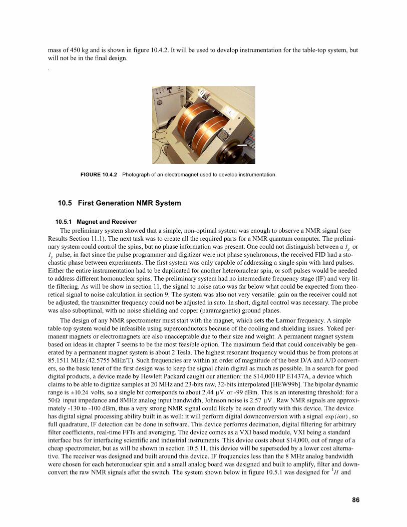
mass of 450 kg and is shown in figure 10.4.2. It will be used to develop instrumentation for the table-top system, but will not be in the final design.
.
10.5 First Generation NMR System
10.5.1 Magnet and Receiver
The preliminary system showed that a simple, non-optimal system was enough to observe a NMR signal (see Results Section 11.1). The next task was to create all the required parts for a NMR quantum computer. The prelimi-nary system could control the spins, but no phase information was present. One could not distinguish between a or
pulse, in fact since the pulse programmer and digitizer were not phase synchronous, the received FID had a sto-chastic phase between experiments. The first system was only capable of addressing a single spin with hard pulses. Either the entire instrumentation had to be duplicated for another heteronuclear spin, or soft pulses would be needed to address different homonuclear spins. The preliminary system had no intermediate frequency stage (IF) and very lit-tle filtering. As will be show in section 11, the signal to noise ratio was far below what could be expected from theo-retical signal to noise calculation in section 9. The system was also not very versatile: gain on the receiver could not be adjusted; the transmitter frequency could not be adjusted in suto. In short, digital control was necessary. The probe was also suboptimal, with no noise shielding and copper (paramagnetic) ground planes.
The design of any NMR spectrometer must start with the magnet, which sets the Larmor frequency. A simple table-top system would be infeasible using superconductors because of the cooling and shielding issues. Yoked per-manent magnets or electromagnets are also unacceptable due to their size and weight. A permanent magnet system based on ideas in chapter 7 seems to be the most feasible option. The maximum field that could conceivably be gen-erated by a permanent magnet system is about 2 Tesla. The highest resonant frequency would thus be from protons at 85.1511 MHz (42.5755 MHz/T). Such frequencies are within an order of magnitude of the best D/A and A/D convert-ers, so the basic tenet of the first design was to keep the signal chain digital as much as possible. In a search for good digital products, a device made by Hewlett Packard caught our attention: the $14,000 HP E1437A, a device which claims to be able to digitize samples at 20 MHz and 23-bits raw, 32-bits interpolated [HEW99b]. The bipolar dynamic range is volts, so a single bit corresponds to about 2.44 or -99 dBm. This is an interesting threshold: for a 50 input impedance and 8MHz analog input bandwidth, Johnson noise is 2.57 . Raw NMR signals are approxi-mately -130 to -100 dBm, thus a very strong NMR signal could likely be seen directly with this device. The device has digital signal processing ability built in as well: it will perform digital downconversion with a signal , so full quadrature, IF detection can be done in software. This device performs decimation, digital filtering for arbitrary filter coefficients, real-time FFTs and averaging. The device comes as a VXI based module, VXI being a standard interface bus for interfacing scientific and industrial instruments. This device costs about $14,000, out of range of a cheap spectrometer, but as will be shown in section 10.5.11, this device will be superseded by a lower cost alterna-tive. The receiver was designed and built around this device. IF frequencies less than the 8 MHz analog bandwidth were chosen for each heteronuclear spin and a small analog board was designed and built to amplify, filter and down-convert the raw NMR signals after the switch. The system shown below in figure 10.5.1 was designed for and
FIGURE 10.4.2 Photograph of an electromagnet used to develop instrumentation.
IxIy
± µ<Ω µ<
iωt( )
H
86

at 0.5 Tesla (21.3 and 5.35 MHz respectively). This software radio approach and simple design is a unique con-tribution.
.
Following the general guidelines for superheterodyne AM receivers, a signal is initially amplified by a low noise figure (1.6 dBm) amplifier with about 27 dB of gain made by Avantek [AVA99] (the UTC103). A wide, coupled-res-onator band-pass filter filters out excessive out of band noise. The next stage is a single component, the RF Microde-vices RF2612, an integrated IF amplifier. It is a general purpose IF amplifier for cellular applications, but the Larmor frequency in this field regime is in the IF frequency regime for many applications. There is a primary stage amplifier that amplifies the signal by 21 dB. The noise figure is considerably higher, but after the first stage as shown in 5.10.2, this is almost insignificant for the overall receiver noise figure. After this, the signal is mixed down to the IF fre-quency from stable, phase locked sources, filtered at the respective IF frequencies with another coupled-resonator fil-ter matched to the 1500 output impedance of the mixer and 1500 input impedance of the next stage. This filter is most critical to the design and should be as tight as possible and offer the most out of band rejection to reject the local oscillator and harmonics of the mixed signals. The bandwidth was set at a wide 500 kHz, and most unwanted out of band signals were later filtered out digitally. The next stage is a variable gain amplifier in the RF2612 that has a gain range -6 to 60 dB with 7 bits of resolution. Finally, a small gain is applied to bring the signals to appropriate levels using a CLC425 fast Op Amp made by Comlinear. The signals are combined in a splitter/combiner made by MA/COM and then sent to the HP E1437A. Overall, this board can attain a maximum gain of 110 dB, with an overall noise figure of about 1.7 dB. With the digitally variable amplifier in the RF Microdevices 2612, the dynamic range of this circuit is about 60 dB. This analog board costs about $400, bringing the total receiver cost to about $14,400.
The actual 2-layer board is shown in figure 10.5.2, with the full schematic in appendix E. A 1mm connector car-ries the 14-bits of information needed to set the amplifier gain on the RF2612. A Pericom 74FCT162244TVA buff-ered line driver helps to filter out some of the noise from the digital interface board (see section 10.5.6). The buffers also have symmetric currents for 0 and 1 states respectively, resulting in a constant output impedance. This helps to prevent ground bounce when switching, reducing system noise. Surface mount ferrite cores were mounted on all power supply lines to filter out any noise at frequencies of interest. The back of the board is a full ground plane, and critical parts such as the first stage low noise amplifier had ground planes on the component sides as well.
FIGURE 10.5.1 General schematic of the analog receiver before interfacing to the HP E1437A. A complete schematic can be found in appendix E.
C
C13 = 5.35 MHz
C13
BPF, BW = 0.5 MHz
HP .1-1000 MHzCW generator
HP 10MHz-20GHzCW generator
7-bit, -7 to 60 dB
Digital Bus Controller(Hitachi 7032 SH1)
To HP 1437
H1 = 21.3 MHzH1
Avantek
27 dB gainNF=1.6 dB
RF2612
21 dB gainNF=4.0 dB
From transmitter13.83 MHz
30 dB gain
Comlinear
15 dB gain
10 dB gain
BPF, BW = 0.5 MHz
7-bit,-7 to 60 dB
Avantek
27 dB gainNF=1.6 dB
RF2612
21 dB gainNF=4.0 dB
ComlinearH1
2 MHz BW
2 MHz BW
From transmitter3 MHz
Ω Ω
87
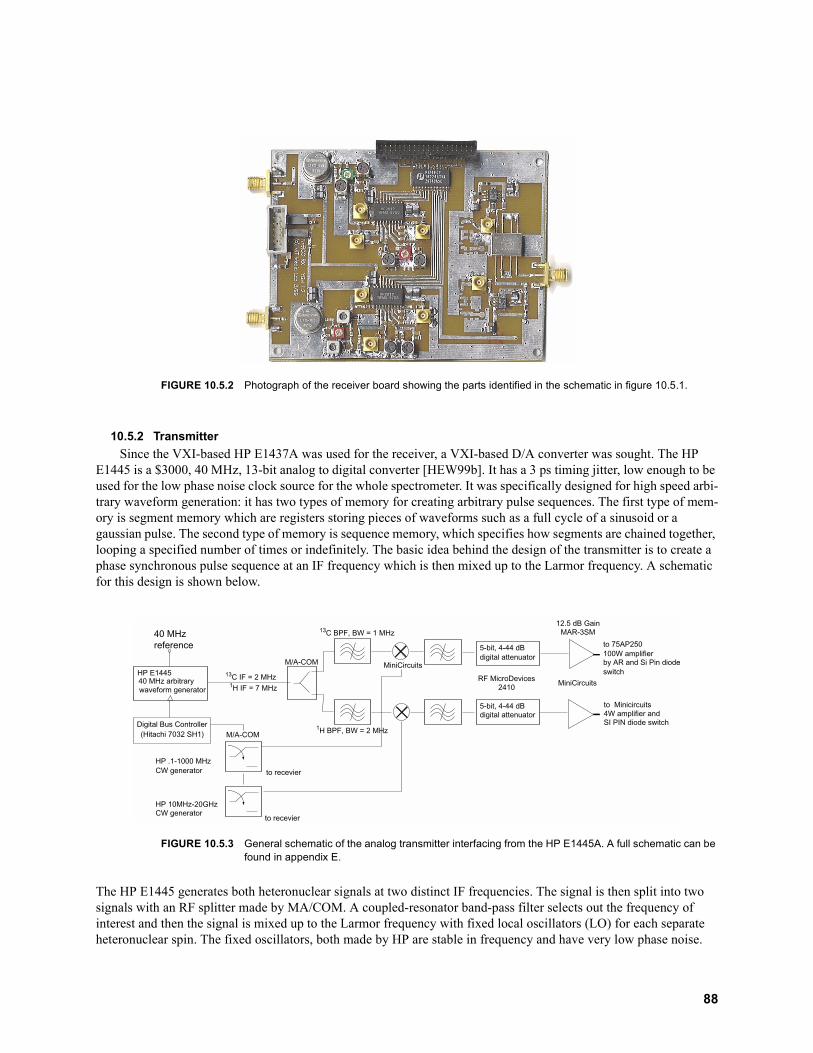
10.5.2 Transmitter
Since the VXI-based HP E1437A was used for the receiver, a VXI-based D/A converter was sought. The HP E1445 is a $3000, 40 MHz, 13-bit analog to digital converter [HEW99b]. It has a 3 ps timing jitter, low enough to be used for the low phase noise clock source for the whole spectrometer. It was specifically designed for high speed arbi-trary waveform generation: it has two types of memory for creating arbitrary pulse sequences. The first type of mem-ory is segment memory which are registers storing pieces of waveforms such as a full cycle of a sinusoid or a gaussian pulse. The second type of memory is sequence memory, which specifies how segments are chained together, looping a specified number of times or indefinitely. The basic idea behind the design of the transmitter is to create a phase synchronous pulse sequence at an IF frequency which is then mixed up to the Larmor frequency. A schematic for this design is shown below.
The HP E1445 generates both heteronuclear signals at two distinct IF frequencies. The signal is then split into two signals with an RF splitter made by MA/COM. A coupled-resonator band-pass filter selects out the frequency of interest and then the signal is mixed up to the Larmor frequency with fixed local oscillators (LO) for each separate heteronuclear spin. The fixed oscillators, both made by HP are stable in frequency and have very low phase noise.
FIGURE 10.5.2 Photograph of the receiver board showing the parts identified in the schematic in figure 10.5.1.
FIGURE 10.5.3 General schematic of the analog transmitter interfacing from the HP E1445A. A full schematic can be found in appendix E.
HP E144540 MHz arbitrarywaveform generator
HP .1-1000 MHzCW generator
HP 10MHz-20GHzCW generator
M/A-COM
M/A-COM MiniCircuits
5-bit, 4-44 dBdigital attenuator
5-bit, 4-44 dBdigital attenuator
RF MicroDevices2410
Digital Bus Controller(Hitachi 7032 SH1)
to recevier
to recevier
to 75AP250100W amplifierby AR and Si Pin diodeswitch
1H IF = 7 MHz
13C IF = 2 MHz
13C BPF, BW = 1 MHz
1H BPF, BW = 2 MHz
to Minicircuits4W amplifier andSI PIN diode switch
40 MHzreference
12.5 dB GainMAR-3SM
MiniCircuits
88
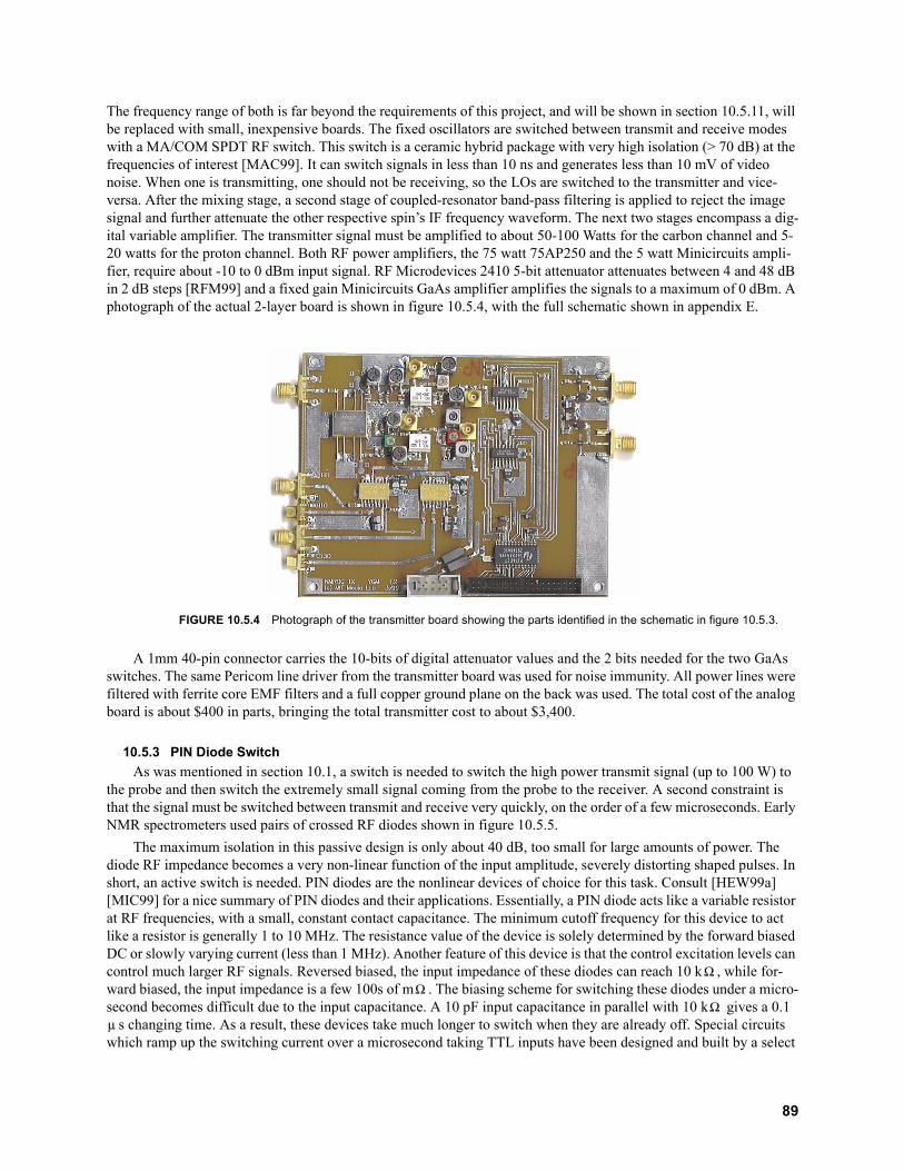
The frequency range of both is far beyond the requirements of this project, and will be shown in section 10.5.11, will be replaced with small, inexpensive boards. The fixed oscillators are switched between transmit and receive modes with a MA/COM SPDT RF switch. This switch is a ceramic hybrid package with very high isolation (> 70 dB) at the frequencies of interest [MAC99]. It can switch signals in less than 10 ns and generates less than 10 mV of video noise. When one is transmitting, one should not be receiving, so the LOs are switched to the transmitter and vice-versa. After the mixing stage, a second stage of coupled-resonator band-pass filtering is applied to reject the image signal and further attenuate the other respective spin’s IF frequency waveform. The next two stages encompass a dig-ital variable amplifier. The transmitter signal must be amplified to about 50-100 Watts for the carbon channel and 5-20 watts for the proton channel. Both RF power amplifiers, the 75 watt 75AP250 and the 5 watt Minicircuits ampli-fier, require about -10 to 0 dBm input signal. RF Microdevices 2410 5-bit attenuator attenuates between 4 and 48 dB in 2 dB steps [RFM99] and a fixed gain Minicircuits GaAs amplifier amplifies the signals to a maximum of 0 dBm. A photograph of the actual 2-layer board is shown in figure 10.5.4, with the full schematic shown in appendix E.
A 1mm 40-pin connector carries the 10-bits of digital attenuator values and the 2 bits needed for the two GaAs switches. The same Pericom line driver from the transmitter board was used for noise immunity. All power lines were filtered with ferrite core EMF filters and a full copper ground plane on the back was used. The total cost of the analog board is about $400 in parts, bringing the total transmitter cost to about $3,400.
10.5.3 PIN Diode Switch
As was mentioned in section 10.1, a switch is needed to switch the high power transmit signal (up to 100 W) to the probe and then switch the extremely small signal coming from the probe to the receiver. A second constraint is that the signal must be switched between transmit and receive very quickly, on the order of a few microseconds. Early NMR spectrometers used pairs of crossed RF diodes shown in figure 10.5.5.
The maximum isolation in this passive design is only about 40 dB, too small for large amounts of power. The diode RF impedance becomes a very non-linear function of the input amplitude, severely distorting shaped pulses. In short, an active switch is needed. PIN diodes are the nonlinear devices of choice for this task. Consult [HEW99a] [MIC99] for a nice summary of PIN diodes and their applications. Essentially, a PIN diode acts like a variable resistor at RF frequencies, with a small, constant contact capacitance. The minimum cutoff frequency for this device to act like a resistor is generally 1 to 10 MHz. The resistance value of the device is solely determined by the forward biased DC or slowly varying current (less than 1 MHz). Another feature of this device is that the control excitation levels can control much larger RF signals. Reversed biased, the input impedance of these diodes can reach 10 k , while for-ward biased, the input impedance is a few 100s of m . The biasing scheme for switching these diodes under a micro-second becomes difficult due to the input capacitance. A 10 pF input capacitance in parallel with 10 k gives a 0.1
s changing time. As a result, these devices take much longer to switch when they are already off. Special circuits which ramp up the switching current over a microsecond taking TTL inputs have been designed and built by a select
FIGURE 10.5.4 Photograph of the transmitter board showing the parts identified in the schematic in figure 10.5.3.
ΩΩ
Ωµ
89
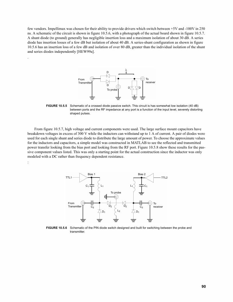
few vendors. Impellimax was chosen for their ability to provide drivers which switch between +5V and -100V in 250 ns. A schematic of the circuit is shown in figure 10.5.6, with a photograph of the actual board shown in figure 10.5.7. A shunt diode (to ground) generally has negligible insertion loss and a maximum isolation of about 30 dB. A series diode has insertion losses of a few dB but isolation of about 40 dB. A series-shunt configuration as shown in figure 10.5.6 has an insertion loss of a few dB and isolation of over 80 dB, greater than the individual isolation of the shunt and series diodes independently [HEW99a].
.
From figure 10.5.7, high voltage and current components were used. The large surface mount capacitors have breakdown voltages in excess of 300 V while the inductors can withstand up to 1 A of current. A pair of diodes were used for each single shunt and series diode to distribute the large amount of power. To choose the approximate values for the inductors and capacitors, a simple model was constructed in MATLAB to see the reflected and transmitted power transfer looking from the bias port and looking from the RF port. Figure 10.5.8 show these results for the pas-sive component values listed. This was only a starting point for the actual construction since the inductor was only modeled with a DC rather than frequency dependent resistance.
:
FIGURE 10.5.5 Schematic of a crossed diode passive switch. This circuit is has somewhat low isolation (40 dB) between ports and the RF impedance at any port is a function of the input level, severely distorting shaped pulses.
FIGURE 10.5.6 Schematic of the PIN diode switch designed and built for switching between the probe and transmitter.
FromTransmitter
Toreceiver
To probe
D
Dλ4_
D D
TTL1
FromTransmitter
TTL2
Toreceiver
To probe
Bias 1 Bias 2
C1 C1L1 L1
C2 C2
L2
D2
D1
D2
D1
90
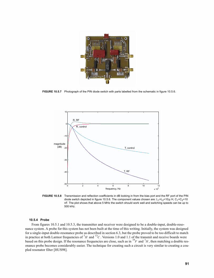
10.5.4 Probe
From figures 10.5.1 and 10.5.3, the transmitter and receiver were designed to be a double-input, double-reso-nance system. A probe for this system has not been built at the time of this writing. Initially, the system was designed for a single-input double-resonance probe as described in section 6.3, but the probe proved to be too difficult to match in practice at both Larmor frequencies of and . Versions 1.0 and 1.1 of the transmit and receive boards were based on this probe design. If the resonance frequencies are close, such as in and , then matching a double res-onance probe becomes considerably easier. The technique for creating such a circuit is very similar to creating a cou-pled resonator filter [HUS98].
FIGURE 10.5.7 Photograph of the PIN diode switch with parts labelled from the schematic in figure 10.5.6.
FIGURE 10.5.8 Transmission and reflection coefficients in dB looking in from the bias port and the RF port of the PIN diode switch depicted in figure 10.5.6. The component values chosen are: L1=L2=10 H, C1=C2=10 nF. The plot shows that above 5 MHz the switch should work well and switching speeds can be up to 500 kHz.
0 2 4 6 8 10 12
x 106
-50
-40
-30
-20
-10
0
10
magnitude(dB)
frequency, Hz
R, RF
R, control
T, control
T, RF
µ
H
C
F$
H
91

Given the 25 mm access gap of the electromagnet, care was exercised to construct a probe box which would accommodate a standard 5 mm NMR tube, while allowing for shim coils and easy access. A probe box was designed to be machined out of standard aluminum using the CAD program Ideas. Ideas outputs g code that can be interpreted by a milling machine to mill the probe box out of a box of aluminum. A photograph of the box and a single input, sin-gle resonance circuit for protons is shown in figure 10.5.9. A small PCB board with ground plane was mounted on the right side of the board to mount the non-magnetic capacitors made by Voltronics [VOL99]. Overall, the inhomoge-neous broadening contribution of this probe was much less than the copper groundplane versions. The sample is interchangeable since the coil was wrapped around a cardboard tube slightly larger than a 5 mm NMR sample tube and epoxied. It is interesting to note that a plastic sample mount was also designed in IDEAS and sent to a 3D ABS plastic printer. However, it turns out the probe was producing a NMR signal without a sample: a reasonable explana-tion was that the protons in the polymer chain of the plastic sample mount were producing a magnetic resonance sig-nal. This was our serendipitous first foray into solid NMR spectroscopy.
10.5.5 Clock Distribution Board
To make the system phase synchronous for generating phased pulses and performing real quadrature detection, all relevant devices needed to be run off of a master clock. The HP E1445A clock reference was chosen for the sys-tem master clock since it has a nice stable, oven controlled crystal reference at 40 MHz with 3 ps timing jitter. The RF generators made by Hewlett Packard both needed 10 MHz references. The HP E1437A and Hitachi microcontroller both needed 20 MHz references. Thus a small clock division board was created using standard logic: a VHC393 dual binary counter, which has low enough timing jitter to be used for this application. The first counter divided the 40 MHz reference to 20 MHz which was split and buffered using a low impedance drive buffer for coaxial cable, a 74F125. The second counter divided the reference to 10 MHz which was also buffered using the 74F125 buffer and sent to the RF generators. A photograph of the actual 2 layer PCB board is shown below in figure 10.5.10, with a schematic in appendix E. The bottom of the board has a complete ground plane. Heavy filtering of the supply lines using ferrite cores and bypass capacitors was implemented.
FIGURE 10.5.9 A single input single resonance probe for protons in an aluminum probe box designed and milled out using the IDEAS CAD program.
92

10.5.6 Digital Interface Board
Both transmitter and receiver require dynamic and static digital information for control. Consulting figure 10.5.3, The HP E1445A needs a trigger to tell the device to start generating the pulse sequence. The GaAs switches need control signals to switch the local oscillators (LO) from the transmitter to the receiver board. The digital attenuators need a total of 10 bits of information. Consulting figure 10.5.1, the receiver needs 14 bits of information for the RF Microdevices 2612 IF amplifiers. For the transmit-receive switch in figure 10.5.6, a pair of dynamic bit were needed for the transmit and receive ends of the switch. Initially, a VXI HP module was tried, the HP E1452 32-bit, 20 MHz Pattern I/O module for $3,000. This device could not be initialized properly and Hewlett Packard technical staff admitted that customers have not been able to get this device working beyond trivial demonstration programs. This device was abandoned in favor of a low cost, 32-bit processor made by Hitachi, the SH-1 7032 [HIT99]. An evalua-tion board, the US7032EDK1 was obtained, shown in figure 10.5.12. A general schematic is shown in figure 10.5.11. This board runs the processor at 20 MHz, contains 128 kB of 70 ns DRAM, a serial port with UART, a 64 kB ultra violet erasable programmable ROM (UVEPROM) and access to 26 pins of general purpose digital I/O. The chip itself has 8 kB of 20 MHz RAM. The device can be programmed via a GNU c-compiler from Cygnus, an industry standard, well maintained set of tools.
FIGURE 10.5.10 Photograph of the actual timing distribution circuit that takes a 40 MHz reference from the HP E1445A, divides it down to 20 MHz and 10 MHz references to be used by other parts of the system. The full schematic can be found in appendix E.
FIGURE 10.5.11 General Schematic of the Hitachi evaluation board, US7032EDK1, used for interfacing to the analog electronics and VXI based modules.
HitachiSH-1
SH7032
MAX232
HostPort
UserPort
ROM RAM RAM
27C512 HN62256BLP-10
93

.
Since there were only 26 pins of general purpose I/O pins, it was decided that instead of multiplexing and adding more digital logic, the system could suffice with only 10 bits of receiver gain control, the remaining 4 bits hard wired. This meant that there would be 20 static bits, 10 each for the transmitter and receiver, and 6 dynamic bits, 2 for switching the local oscillators between transmit and receive, 2 for controlling the PIN diode switches and 2 for trig-gering the HP VXI A/D and D/A converters. The 20 static bits could easily be programmed in the Hitachi, simply by setting register values at run time through a serial port. The dynamic bits were slightly trickier since one needed very precise timing control throughout an experiment. Most critical of all is the time between the start trigger of the HP E1445 device that starts the pulse sequence and the start trigger of the HP E1437A, which starts the data acquisition. Since the E1437A performs quadrature detection and digital downsampling, for the phase to be preserved between and during experiments, this time duration must be both precise and accurate. Thus, the clock distribution board in section 10.5.5 creates a 20 MHz reference clock for the Hitachi processor.
In terms of the software, to create precise timing control without consuming egregious amount of memory, a tim-ing and state vector are specified: and . Each index is a 32-bit number spec-ifying a time in arbitrary units and each uses 8-bits to specify the state of all 6 pins. A tight inlined function loops until a counter reaches , then the state of each pin is written with the state . For code that was executed from the external UVEPROM and RAM, the effective clock speed was about 2 MHz, and with algorithmic overhead, the tim-ing resolution became 2.5 . To get the timing resolution down to sub microsecond levels, the entire code had to be moved to the on-chip RAM. This was a very complicated process which involved booting the code of the external UVEPROM and then getting the code to copy itself into the on chip RAM. The gains were impressive: the timing res-olution became 250 ns. The actual NMR pulse programming code, detailed in appendix F was written with another student Edward Boyden [BOY99]. The implementation code for copying code to on-chip RAM was implemented by Rehmi Post. Programming of the state vector and messages to start the pulse program were programmed over the serial port via programs written in the C programming language [BOY99].
Digital circuitry is always substantially noisy, too noisy in fact to interface directly to the sensitive receiver and transmitter. Thus a few steps were taken to help reduce noise contributions from the digital circuit: separate power and ground lines were created for the digital circuitry; integrated R-C low pass filters were placed on the output pin of each digital output line; line buffers were supplied on the transmitter and receiver boards to try to filter out any noise in the signal. For digital lines that needed to drive coaxial cable and 50 loads at TTL levels, high current 74F125 buffers were used. Each chip contained 4 buffers, so two sufficed for the six coaxial lines. A board with the RC filter-
FIGURE 10.5.12 Hitachi evaluation board used for pulse programming and system control.
ττττ τ τ τ …, , ,( ) σσσσ σ σ σ …, , ,( ) τiσi
τi σi
µ
Ω
94

ing, connector outputs and buffering for 50 coaxial cable is shown in figure 10.5.13, with the detailed schematic found in appendix E.
.
10.5.7 Power Board
Integral to the performance of the overall system is a need for a good supply and grounding. To get a working system running as soon as possible, a digitally controlled power supply, the HP E3631A was used. The voltages needed were analog +5V, -5V, digital +5V and separate grounds for both analog and digital supplies. A small inter-face board was created to take the signals from the HP E3631A and send them to the various boards. Standard 2mm IDC connectors were being used to carry power. Regulators and 1000 capacitors were used on each of the sepa-rate lines to filter out any noise or 60 cycle a.c influences. A photograph of the actual 2 layer board is shown in figure 10.5.14, the system schematic shown in appendix E. A separate connector was needed for: the transmitter, receiver, the digital interface board and the clock distribution board.
FIGURE 10.5.13 Photograph of the digital interface board. Each digital line from the Hitachi evaluation board (top grey connectors) are filtered with integrated RC resonators (middle components) and output to the transmitter and receiver boards (black connectors). On the right are a pair of 74F125s to drive the six 50 coaxial cables. A schematic can be found in appendix E.
FIGURE 10.5.14 Photograph of the PCB board fabricated for doing power distribution. The power lines come in from the HP E3631A to a standard header connector on the bottom, or regulated and bypassed with large 1000 F capacitors to the separate 2mm IDC connectors above. The detailed schematic can be found in appendix E.
Ω
Ω
µ
µ
95
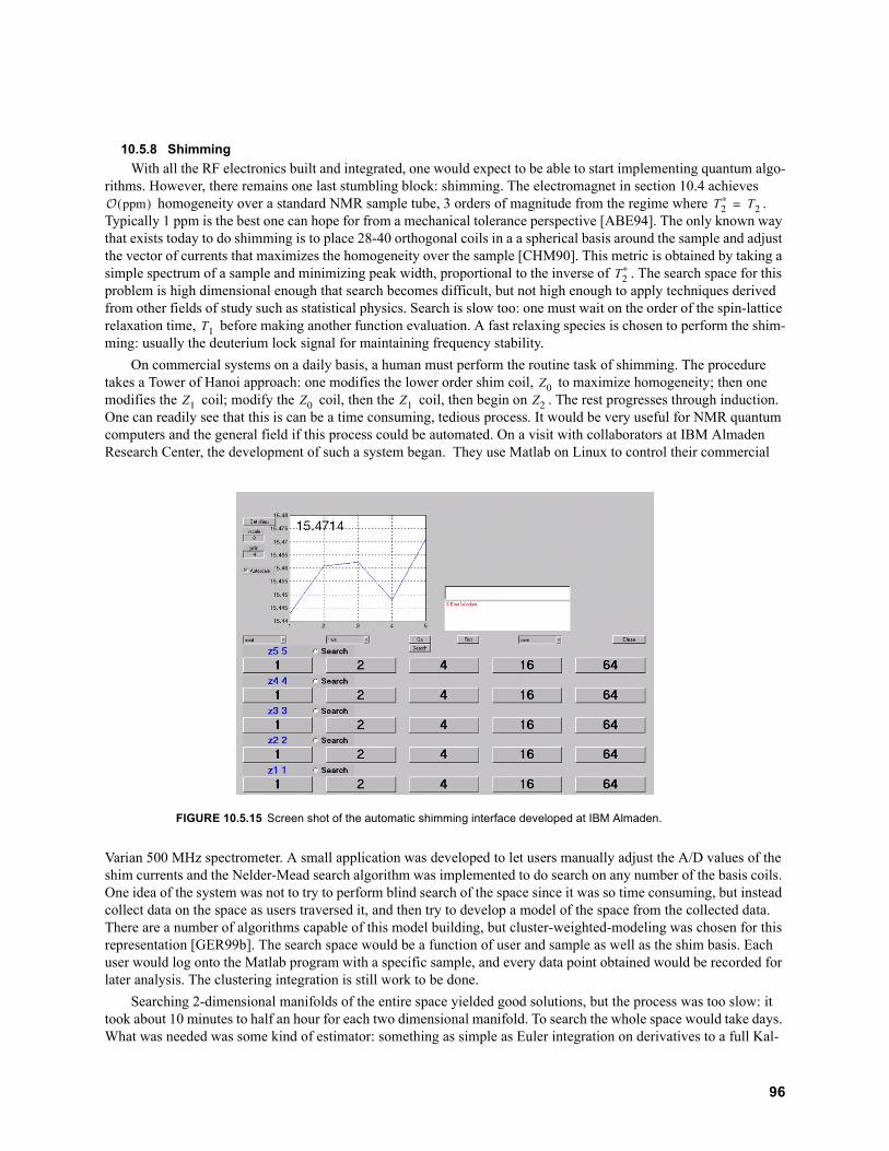
10.5.8 Shimming
With all the RF electronics built and integrated, one would expect to be able to start implementing quantum algo-rithms. However, there remains one last stumbling block: shimming. The electromagnet in section 10.4 achieves
homogeneity over a standard NMR sample tube, 3 orders of magnitude from the regime where . Typically 1 ppm is the best one can hope for from a mechanical tolerance perspective [ABE94]. The only known way that exists today to do shimming is to place 28-40 orthogonal coils in a a spherical basis around the sample and adjust the vector of currents that maximizes the homogeneity over the sample [CHM90]. This metric is obtained by taking a simple spectrum of a sample and minimizing peak width, proportional to the inverse of . The search space for this problem is high dimensional enough that search becomes difficult, but not high enough to apply techniques derived from other fields of study such as statistical physics. Search is slow too: one must wait on the order of the spin-lattice relaxation time, before making another function evaluation. A fast relaxing species is chosen to perform the shim-ming: usually the deuterium lock signal for maintaining frequency stability.
On commercial systems on a daily basis, a human must perform the routine task of shimming. The procedure takes a Tower of Hanoi approach: one modifies the lower order shim coil, to maximize homogeneity; then one modifies the coil; modify the coil, then the coil, then begin on . The rest progresses through induction. One can readily see that this is can be a time consuming, tedious process. It would be very useful for NMR quantum computers and the general field if this process could be automated. On a visit with collaborators at IBM Almaden Research Center, the development of such a system began. They use Matlab on Linux to control their commercial
Varian 500 MHz spectrometer. A small application was developed to let users manually adjust the A/D values of the shim currents and the Nelder-Mead search algorithm was implemented to do search on any number of the basis coils. One idea of the system was not to try to perform blind search of the space since it was so time consuming, but instead collect data on the space as users traversed it, and then try to develop a model of the space from the collected data. There are a number of algorithms capable of this model building, but cluster-weighted-modeling was chosen for this representation [GER99b]. The search space would be a function of user and sample as well as the shim basis. Each user would log onto the Matlab program with a specific sample, and every data point obtained would be recorded for later analysis. The clustering integration is still work to be done.
Searching 2-dimensional manifolds of the entire space yielded good solutions, but the process was too slow: it took about 10 minutes to half an hour for each two dimensional manifold. To search the whole space would take days. What was needed was some kind of estimator: something as simple as Euler integration on derivatives to a full Kal-
FIGURE 10.5.15 Screen shot of the automatic shimming interface developed at IBM Almaden.
,( ) T T
T
T
ZZ Z Z Z
96

man filter. With an estimator and compact representation of the space, this could be a starting point for the develop-ment of a useful tool. From a user interface perspective, there is also much work to be done. A novel interface to the spectrometer via a joystick was developed in Matlab. However, since the code was interpreted and Matlab does not support multithreading, the user-interface was unresponsive and difficult to interact with. For our spectrometer, the essential code will be moved to the Java programming language, allowing multithreading but still maintaining plat-form universality.
10.5.9 The Whole Picture
Integrating all the work outlined in sections 10.5.1 through , the overall system schematic is as shown in figure 10.5.16.
The customized electronics boards were placed in a steel rack mounted case. The receiver board was placed in another aluminum box to shield against stray signals. The whole system was then mounted in a rack mount shelf with signal generators, PIN diode switches and power supplies. The shim circuit boards were mounted in a separate box, mounted near the magnet.
FIGURE 10.5.16 Overall system schematic for the current NMR spectrometer. Items with a box indicate items that have been designed in-house. Items with a box indicate items that are running off the power distribution board (lower right). The indicates chilled water.
HP E1445Arb. wavegenerator
SH7032EDK132-bit pulseprogrammer
Clockdistribution
40 MHzreference
20 MHzreference
Trigger
12
14
Digital Interface
Transmit board
12:2 LO switch10 digital attenuator
AR 75AP25075 W, RF AmpVXI
MC TIA-1000-1R8 5 W, RF Amp
RS232
PIN diodeDPDT switch
PIN diodeDPDT switch
4:2 Transmit2 Receive
HP 8648A.1-1000 MHz
LO
HP 83172B10-20000 MHz
LO
13C IF
1H LO13C LO
13C ω
1H ω19F ω
1H IF19F IF
Probe
Electromagnet
HP E143723-bit A/Dconverter
Receive board
10 MHz reference
10: digital amplifier
VXI
DANFYSKPower Supply
Bay VoltexHeat Exchanger
Housechilled water
70 AHP 6614C
Power Supply
-100V
PowerDistribution
HP E3631APower Supply
Shim
Shim Board
RS232
VXI, HP E8400A
VXI I/O
PC, 200 MHzPentium Pro
RS232 I/O
97

10.5.10 Software
Control of the software effort for this project was maintained and developed primarily by Edward Boyden and is well detailed in his thesis [BOY99]. As one could imagine, the software undertaking for this project is quite substan-tial. From a top down approach, the final goal of this project will be to treat the NMR instrumentation as a real com-puter. That is, one would like to be able to write a program in a programming language and then compile this code down to native instructions or a pulse sequence for the spins. There are many challenges to making this happen: Ini-tially, one must figure out how to compile a quantum algorithm down to pulses or elementary unitary operations in an efficient manner. By efficient, if implemented on a classical computer, compilation must not consume exponential amounts of time or space or the whole effort of quantum computation will be lost. Efficient means also arranging a pulse sequence to take advantage of the architecture at hand. In a classical computer where integer multiplies might be very efficiently implemented in hardware over other mathematical functions, it makes sense for a compiler to take advantage of this to best optimize an algorithm. Similarly in quantum computers, it makes sense to look for spins that have higher J-coupling constants for faster gates, slower relaxation times or look for symmetries in a pulse sequence that potentially cancel out particular pulses from a dynamical or average Hamiltonian perspective. In classical com-puters, when a compiler is written for a specific architecture, those machine dependencies are included in the com-piler. It would be nice to go beyond that and allow the system itself to determine it’s own optimizations. By taking two dimensional spectra, it is conceivable to determine the Hamiltonian of the system through careful peak determi-nation and certain levels of heuristics that people use to interpret these plots. These are all nascent goals but are a use-ful guide for what to expect from these machines in the future and a starting point for software design.
Starting from the bottom up, the programming for the pulse programmer was specified in section 10.5.6 and appendix F. The HP E1445 and E1437 devices both had to be programmed. Hewlett Packard supplied Win32 dynamic link libraries (DLLs) for communicating with these devices in a Windows 95/98 environment. These pro-gramming model for these devices must comply to a standard set of instructions called VISA. VISA then talks over another programming language called SICL which each device natively understands. For the HP E1445, very non-trivial development was made so that arbitrarily shaped, phased pulses could be generated. Since only one manually controlled local oscillator per channel was available, one could not simply change the phase of the local oscillator by
to get and terms, as is done commercially. Since we were generating the IF directly on a single channel, the phase of the transmitter itself is very important to generate phase in the transmitter. The problem compounds when one tries to implement pulses. Consider trying to implement the following simple pulse sequence:
The problem is that to implement the delay and then apply the pulse requires timing resolution to a subcy-cle of the Larmor frequency on the HP E1445. At 1 T, for protons with a Larmor frequency of 42.5755 MHz, the 40 MHz reference of the E1445 is too coarse to be able to specify any reasonable phase accuracy. Fortunately an D/A not only has timing precision but amplitude precision. By leveraging the 13-bits of amplitude resolution, one can precal-culate what the starting phase of the sine wave should be to obtain the pulse. This presents a lot of work for the software for the HP E1445 since for each pulse, one must specify a different starting position in the sequence mem-ory. Considering the small amount of both sequence and segment memory, this posed a difficult challenge, especially when trying to make shaped gaussian pulses. However, within a few hundred bytes of the maximum amount of sequence and segment RAM, the task was completed, as outlined in [BOY99].
The second remaining software undertaking was the development of the receiver software. Initially software was written in the C programming language to communicate to the E1437A, as was the E1445. Unfortunately, there were several bugs that could not be resolved in an efficient manner, so instead of trying to figure out what was incorrect, our efforts were leveraged by modifying a sample program provided by Hewlett Packard. A small piece of the code was modified for our purposes to save the state of an experiment as complex, 32-bit data in a binary file. This demon-stration program already had a nice set of tools for running experiments: a logarithmic frequency display, support for external triggers and digital filtering control. This software was written by the author in Visual Basic 6.0.
FIGURE 10.5.17 A simple two pulse experiment that proved to be very difficult to implement with the current transmitter
$
Ix Iy
90x
τ
90y
τ $y
$y
98
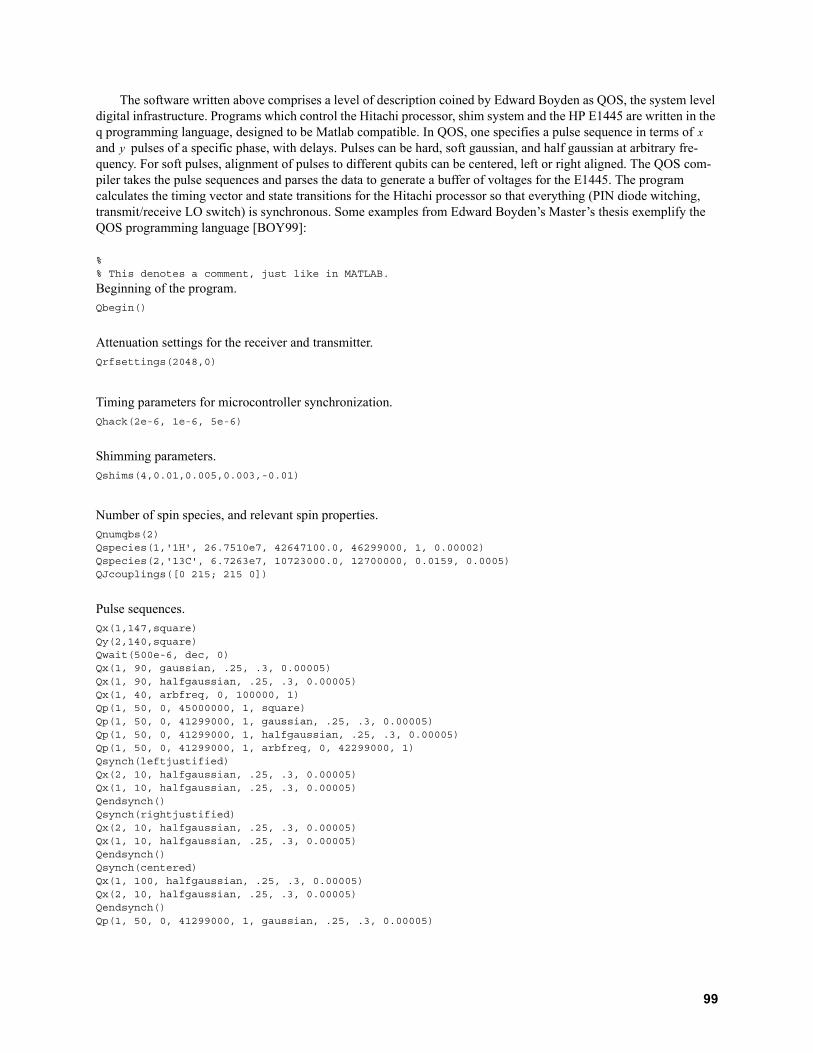
The software written above comprises a level of description coined by Edward Boyden as QOS, the system level digital infrastructure. Programs which control the Hitachi processor, shim system and the HP E1445 are written in the q programming language, designed to be Matlab compatible. In QOS, one specifies a pulse sequence in terms of and pulses of a specific phase, with delays. Pulses can be hard, soft gaussian, and half gaussian at arbitrary fre-quency. For soft pulses, alignment of pulses to different qubits can be centered, left or right aligned. The QOS com-piler takes the pulse sequences and parses the data to generate a buffer of voltages for the E1445. The program calculates the timing vector and state transitions for the Hitachi processor so that everything (PIN diode witching, transmit/receive LO switch) is synchronous. Some examples from Edward Boyden’s Master’s thesis exemplify the QOS programming language [BOY99]:
%% This denotes a comment, just like in MATLAB.
Beginning of the program.
Qbegin()
Attenuation settings for the receiver and transmitter.
Qrfsettings(2048,0)
Timing parameters for microcontroller synchronization.
Qhack(2e-6, 1e-6, 5e-6)
Shimming parameters.
Qshims(4,0.01,0.005,0.003,-0.01)
Number of spin species, and relevant spin properties.
Qnumqbs(2)Qspecies(1,'1H', 26.7510e7, 42647100.0, 46299000, 1, 0.00002)Qspecies(2,'13C', 6.7263e7, 10723000.0, 12700000, 0.0159, 0.0005)QJcouplings([0 215; 215 0])
Pulse sequences.
Qx(1,147,square)Qy(2,140,square)Qwait(500e-6, dec, 0)Qx(1, 90, gaussian, .25, .3, 0.00005)Qx(1, 90, halfgaussian, .25, .3, 0.00005)Qx(1, 40, arbfreq, 0, 100000, 1)Qp(1, 50, 0, 45000000, 1, square)Qp(1, 50, 0, 41299000, 1, gaussian, .25, .3, 0.00005)Qp(1, 50, 0, 41299000, 1, halfgaussian, .25, .3, 0.00005)Qp(1, 50, 0, 41299000, 1, arbfreq, 0, 42299000, 1)Qsynch(leftjustified)Qx(2, 10, halfgaussian, .25, .3, 0.00005)Qx(1, 10, halfgaussian, .25, .3, 0.00005)Qendsynch()Qsynch(rightjustified)Qx(2, 10, halfgaussian, .25, .3, 0.00005)Qx(1, 10, halfgaussian, .25, .3, 0.00005)Qendsynch()Qsynch(centered)Qx(1, 100, halfgaussian, .25, .3, 0.00005)Qx(2, 10, halfgaussian, .25, .3, 0.00005)Qendsynch()Qp(1, 50, 0, 41299000, 1, gaussian, .25, .3, 0.00005)
xy
99

Data acquisition command.
Qread(100e-6,dec,0)
End of program.
Qend()
The QOS programming language itself contains thousands of lines of code. To make this code more manageable and extensible, the code has recently been moved to an object framework using the C++ programming language. The ability to access this software on many platforms is paramount for development, so we have wrapped our windows software into Java using the Java Native Interface. This allows us to access our server machine interfacing to our hardware over IP (Internet Protocol) in a hardware abstract manner. An example of a simple program to control the 1445 is given in appendix G. Raefer Gabriel, a student working here has implemented the full QOS architecture in Java using JNI and RMI.
For the next level of description in software, it would be useful to try to automate some standard NMR processes to begin to make the system seem more like a basic computer rather than a NMR spectrometer. Countless hours are spent by spectrometer users and technicians, performing shimming to maximize spectral sensitivity. It would be nice to perform continuous online shimming to make sure that the shim current distribution is always at a local minimum in terms of peak width. Since the shimming space is a very non-linear high dimensional space, efficient search algo-rithms are needed. To extract useful quantitative information requires a lot of calibration: creating a pulse requires creating an experiment to generate the plot shown in figure 6.1.1. Doing state tomography requires measur-ing the area under peaks representing various terms of the density matrix. It would be useful to have a number of rou-tines to measure parameters of peaks in frequency space using linear and non-linear function fitting to perform automatic data extraction. Edward Boyden has developed such a package, ROS (the next letter after Q) to take a q program, apply a certain method such as Powell’s direction set method, the downhill simplex method, brute-force search, conjugate gradient descent [PRE93] or cluster weighted modeling [GER99a] to achieve a specific goal. The set of goals can be to maximize signal-to-noise, maximize , maximize sharpness of a certain peak and so forth [BOY99].
10.5.11 Future Work
As is shown in the results section of section, it is the belief of this author that the current generation NMR system will lead to the ability to perform simple quantum algorithms. However, looking at the system diagram in figure 10.5.16 this system can hardly be considered table-top. Section 7 on magnet design shows theoretical means for replacing the bulky electromagnet, but still more electronics development needs to be done to reduce the electronics complexity. Most of the problems in the design of the current system revolve around the transmitter and the compli-cations of generating phased waveforms thereof. It is also necessary to replace the costly and bulky RF synthesizers and the whole VXI interface if possible. Fortunately, the blistering pace of the electronics industry has rendered most of this bulky hardware to a couple of integrated circuits.
The entire transmitter chain can essentially be replaced by a single chip: the AD9856 made by Analog Devices [ANA99]. This chip takes 12 bit complex data and performs quadrature upconversion digitally and then outputs to a 12-bit 200 MHz digital to analog converter (DAC). It has integrated digital filters and a clock multiplier all built into the chip, while still offering excellent phase noise characteristics. The input bandwidth of the signal in can be maxi-mally 4 times less than the internal system clock, which can run up to 200 MHz. To provide the 12-bit complex data into the AD9856, at reasonable data rates (> 10 Msps), would require a time-space tradeoff. The time constraining solution would be to use a 32-bit Hitachi microprocessor and a large amount of memory to store the processed wave-forms. As in the same paradigm of the HP E1445A, segment and sequence memory would be supplied, but here the demands on the system would be much less difficult since the whole system would be made from the ground up to be a quadrature upconverter. The space constrained system would use very fast processor running at over 200 MHz that would compute the A/D values on the fly. A number of vendors such as Hitachi, Intel or simply FPGA’s are possible solutions. Either way this system would also be substantially cheaper and would allow for separate transmitters for each heteronuclear species. A simplified schematic is shown in figure 10.5.18, revealing a board that should only cost a few hundred dollars. Edward Boyden began development of such a transmitter using a different paradigm, field pro-grammable gate arrays (FPGAs). His “nanoNMR” is outlined in his Master’s Thesis [BOY99].
$x
T
100
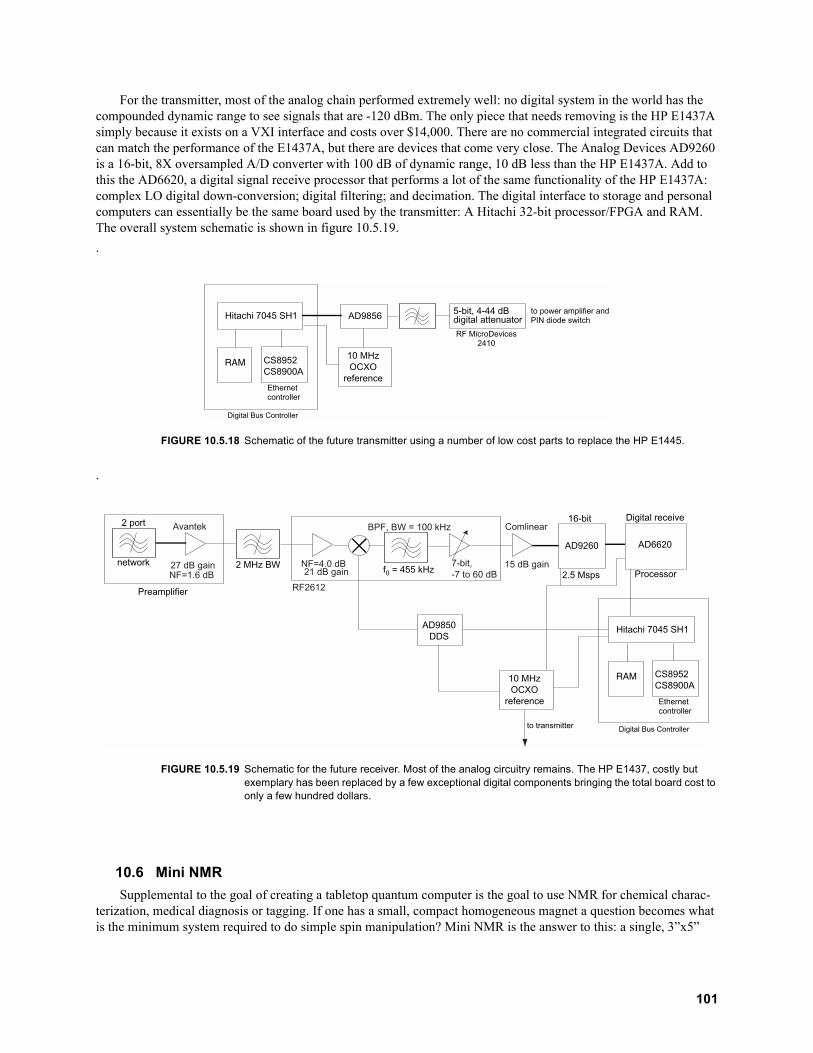
For the transmitter, most of the analog chain performed extremely well: no digital system in the world has the compounded dynamic range to see signals that are -120 dBm. The only piece that needs removing is the HP E1437A simply because it exists on a VXI interface and costs over $14,000. There are no commercial integrated circuits that can match the performance of the E1437A, but there are devices that come very close. The Analog Devices AD9260 is a 16-bit, 8X oversampled A/D converter with 100 dB of dynamic range, 10 dB less than the HP E1437A. Add to this the AD6620, a digital signal receive processor that performs a lot of the same functionality of the HP E1437A: complex LO digital down-conversion; digital filtering; and decimation. The digital interface to storage and personal computers can essentially be the same board used by the transmitter: A Hitachi 32-bit processor/FPGA and RAM. The overall system schematic is shown in figure 10.5.19.
.
.
10.6 Mini NMR
Supplemental to the goal of creating a tabletop quantum computer is the goal to use NMR for chemical charac-terization, medical diagnosis or tagging. If one has a small, compact homogeneous magnet a question becomes what is the minimum system required to do simple spin manipulation? Mini NMR is the answer to this: a single, 3”x5”
FIGURE 10.5.18 Schematic of the future transmitter using a number of low cost parts to replace the HP E1445.
FIGURE 10.5.19 Schematic for the future receiver. Most of the analog circuitry remains. The HP E1437, costly but exemplary has been replaced by a few exceptional digital components bringing the total board cost to only a few hundred dollars.
5-bit, 4-44 dBdigital attenuator
RF MicroDevices2410
Digital Bus Controller
Hitachi 7045 SH1 to power amplifier andPIN diode switch
RAM
Ethernetcontroller
CS8952CS8900A
AD9856
10 MHzOCXO
reference
BPF, BW = 100 kHz
7-bit, -7 to 60 dB
Avantek
27 dB gainNF=1.6 dB
RF2612
21 dB gainNF=4.0 dB
Comlinear
15 dB gain2 MHz BW
AD9850DDS
f0 = 455 kHz
Preamplifier
2 port
network
AD9260
16-bit
2.5 Msps
Digital Bus Controller
Hitachi 7045 SH1
RAM
Ethernetcontroller
CS8952CS8900A
AD6620
Digital receive
Processor
10 MHzOCXO
reference
to transmitter
101

board that is capable of generating simple pulse sequences and switches to a low noise receiver for detecting the tiny NMR signals, as shown in figure 10.6.1. A schematic is shown in figure 10.6.2.
The board is controlled by a PC over serial RS-232 protocol to a Microchip PICF84. The PIC sends commands to the AD9850, a 125 MHz, complete CMOS direct digital synthesizer (DDS). This device generates sinusoids with 32-bit frequency resolution up to 40 MHz. Controlling the Minicircuits ASW-2-50DR SPDT switch allows one to imple-ment pulses and the second switch controls DDS output between transmit and receive [MIN99]. This system is designed for less than 0.5 W of transmit power, so it can only be used for proton spins.
.
FIGURE 10.6.1 Photograph of a complete NMR spectrometer, MiniNMR.
FIGURE 10.6.2 Schematic of Mini NMR revealing the small number of low cost parts needed to implement basic NMR functionality.
FREQUENCYSOURCE
AD9850 DDS
R.F GateMini-Circuits
Scos(ωot)A
r.f. power amp, 0.25 W (AD811)
r.f GateMini-Circuits
Mini-circuits, MAN-1LN
TX
RX
PulseProgrammer
PICF84
RS-232MAX233
to probe
ASW-2-50DR
LPFBuffer
ComlinearCLC-425
Mini-circuitsSRA-3MH
102

11.
Results
11.1 Old System
For the preliminary system with electromagnet, the design goals were simple: to show control over a single spin on a molecule in the ensemble; and then to show control via -coupling that interaction could be observed, necessary for implementing gates like CNOTs. The first demonstration was to take 0.2 cm3 of isopropanol in a standard 5mm NMR tube and apply a broadband pulse to the spins. Since the system was not phase synchronous, the axis of rotation is a stochastic variable. Nevertheless, this simple experiment was done, and data was collected showing peak separation on the order of 50 Hz. This is shown in figure 11.1.1. The signal to noise ratio, 16 is quite low – not sur-prising given the hardware but demonstrative of basic principles.
The next task was to observe -coupling. About 0.2 cm3 of liquid chloroform in a 5 mL ampule from Cambridge Isotope Laboratories was used with no solvent, and a single pulse, was applied to the proton spins. The
causes a =215 Hz splitting in the normal single peak. This was observed and is shown in figure 11.1.2. It was imperative to prove this was scalar coupling, and three basic tests will reveal this: a CPMG sequence will remove chemical shift evolution and the decay envelope would be modulated by the coupling; changing the magnetic field ( -coupling is not a function of the static field); or perform a 2D correlation experiment. The last method was chosen simply to get experience in 2D NMR. The plot shows just one corner of the plot from figure 3.4.2, but the peak sepa-ration of the diagonal is evident.
FIGURE 11.1.1 Demonstration of chemical shifts in isopropanol. S/N = 16 (single shot).
J
Rxπ---
-4800 -4700 -4600 -4500 -4400 -4300 -42000
0.05
0.1
0.15
0.2
0.25
0.3
0.35
0.4
0.45
ampl
itude
, a.u
.
frequency offset from L.O. (Hz)
JRx
π---
πJt( ) J
JJ
103

11.2 New System
With these simple demonstrations, the new system was designed to address the issues of: addressing multiple spins, signal to noise ratio; phase coherent signal transmission and detection; and quadrature detection. This system is much more complicated than the preliminary system, but from section 10.5, should be complete for doing quantum computation. Some preliminary result are shown below in figures 11.2.1 and 11.2.2. The first plot, on a logarithmic scale shows the dramatic increase in the signal to noise ratio of the proton signal, well over 50 dB. The sample is a 50% solution of glycerine in water. The sample volume is again 0.2 cm3 in a standard 5 mm NMR sample tube. The
FIGURE 11.1.2 Demonstration of J-coupling in chloroform in the proton spectrum. The measured splitting is 225 ± 10 Hz. S/N = 8 (single shot).
FIGURE 11.1.3 A correlation spectroscopy experiment to prove that J-coupling was observed.
-14.5 -14 -13.5 -13 -12.5 -12 -11.5-1
-0.5
0
0.5
1
1.5
2
Frequency offset from L.O. (kHz)
ampl
itude
(a.
u.)
10002000
30004000
50006000
1820
1840
1860
1880
1900
1920-2000
-1000
0
1000
2000
3000
4000
f2, Hzf1, Hz
Am
plitu
de (
a.u.
)
104

average spin signal over the detection period is about -65 dBm. The data collection time (3.28 ms) was short, but on the order of inhomogeneously broadened decoherence time . The second plot shows the improvement in -cou-pling in both sensitivity and frequency resolution. Peaks can now be fully distinguished – they are not the two humps shown in 11.1.2. The signal to noise ratio (50) is substantially less than the glycerine signal of figure 11.2.1. This is due to a couple of factors. The first is that in order to observe the splitting of the peaks, the data had to be collected for several periods (about 10), which severely reduces the sensitivity. The second reason is that chloroform has less intrinsic sensitivity than the glycerine-water solution. Matching the same observation time and bandwidth yields a signal to noise ratio of about 40 dB, 10 dB less than the glycerine-water solution. These are all preliminary results – shimming is paramount for further progress to developing a table-top quantum computer.
FIGURE 11.2.1 Plot showing the sensitivity of the proton spectrum of water. Data was collected for 3.28 ms at a bandwidth of 122070.32 Hz.
T J
T
105

FIGURE 11.2.2 J coupling on the new spectrometer and new probe on a logarithmic scale. The full splitting of the peaks can be seen with better S/N = 50 (singe shot).
106
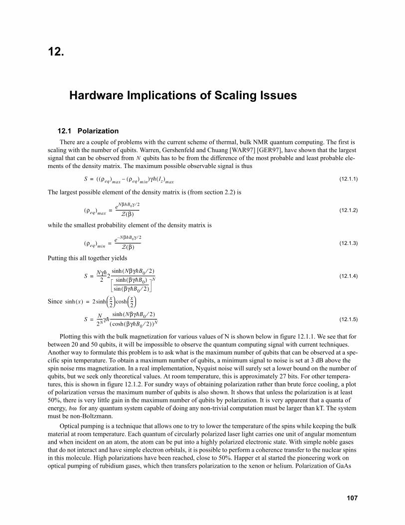
12.
Hardware Implications of Scaling Issues
12.1 Polarization
There are a couple of problems with the current scheme of thermal, bulk NMR quantum computing. The first is scaling with the number of qubits. Warren, Gershenfeld and Chuang [WAR97] [GER97], have shown that the largest signal that can be observed from qubits has to be from the difference of the most probable and least probable ele-ments of the density matrix. The maximum possible observable signal is thus
(12.1.1)
The largest possible element of the density matrix is (from section 2.2) is
(12.1.2)
while the smallest probability element of the density matrix is
(12.1.3)
Putting this all together yields
(12.1.4)
Since
(12.1.5)
Plotting this with the bulk magnetization for various values of N is shown below in figure 12.1.1. We see that for between 20 and 50 qubits, it will be impossible to observe the quantum computing signal with current techniques. Another way to formulate this problem is to ask what is the maximum number of qubits that can be observed at a spe-cific spin temperature. To obtain a maximum number of qubits, a minimum signal to noise is set at 3 dB above the spin noise rms magnetization. In a real implementation, Nyquist noise will surely set a lower bound on the number of qubits, but we seek only theoretical values. At room temperature, this is approximately 27 bits. For other tempera-tures, this is shown in figure 12.1.2. For sundry ways of obtaining polarization rather than brute force cooling, a plot of polarization versus the maximum number of qubits is also shown. It shows that unless the polarization is at least 50%, there is very little gain in the maximum number of qubits by polarization. It is very apparent that a quanta of energy, for any quantum system capable of doing any non-trivial computation must be larger than kT. The system must be non-Boltzmann.
Optical pumping is a technique that allows one to try to lower the temperature of the spins while keeping the bulk material at room temperature. Each quantum of circularly polarized laser light carries one unit of angular momentum and when incident on an atom, the atom can be put into a highly polarized electronic state. With simple noble gases that do not interact and have simple electron orbitals, it is possible to perform a coherence transfer to the nuclear spins in this molecule. High polarizations have been reached, close to 50%. Happer et al started the pioneering work on optical pumping of rubidium gases, which then transfers polarization to the xenon or helium. Polarization of GaAs
N
S ρeq( )max
ρeq( )min
( )γ! Iz( )max
ρeq( )max
eNβ!Bγ ⁄
β( )------------------------
ρeq( )min
e N β!Bγ ⁄
β( )--------------------------
SNγ!
----------Nβγ!B ⁄( )
βγ!B( )
βγ!B ⁄( )-----------------------------------
N---------------------------------------------
x( ) x---
x---
SNN------γ!
Nβγ!B ⁄( )
βγ!B ⁄( )( )N------------------------------------------------
!ω
107

substrates [PAG81] at low temperatures has been achieved, but little progress has been made polarizing liquids. This is a difficult process since the normal nuclei used in NMR cannot be optically addressed directly. The only way to enhance the polarization is through cross polarization by cross relaxation with another species. As it exists now, it is cumbersome: laser pumped rubidium transfers polarization by a van der walls molecule formation to or to obtain polarization. The polarized or then cross relaxes with the NMR species. This multi-stage pro-cess should have fundamental problems getting close to unity polarization for the NMR nuclei based on the cross relaxation rates involved. However for NMR, order unity polarization by optical pumping or other means is essential for quantum computing to scale. Not only for signal to noise concerns as will be shown below but also essentially for
quantum error correction. As ancillary qubits are entangled with those performing a computation and then released containing the errors, for errors to not be reintroduced into the system, they must be cooled to the ground state. Con-tinuous state preparation by cooling is a necessity.
FIGURE 12.1.1 Observable magnetization and the ideal quantum computing signal at a function of temperature. Also shown is the fundamental rms spin noise magnetization, for 1022 particles at a resonance frequency of 600 MHz.
FIGURE 12.1.2 Left is a plot of maximum number of qubits obtainable as a function of temperature to have a S/N of 3dB relative to the spin noise. On the right is a plot of polarization versus maximum number of qubits.
H
Xe$
( ) H
Xe$
10-2 10-1 100 101 10210-35
10-30
10-25
10-20
10-15
10-10
10-5
100
Magnetization
N=5N=10
N=20
N=50
N=100
spin noise
mag
netiz
atio
n
Temperature (K)
10-2 10-1 100 101 102 1030
50
100
150
200
250
300
350
400
450
500
Temperature(K)
Max
imum
Num
ber
of Q
ubits
102
103
10-4
10-3
10-2
10-1
100
Pol
ariz
atio
n
Maximum Number of Qubits
108

12.1.1 Another approach to scalable quantum computing
Leonard Shulman and Umesh Vazirani have come up with another technique to implement quantum computing [SHU98]. It is a technique more scalable than the ones proposed thus far in that the intrinsic signal to noise ratio of the system does not change with the size of the computer. The technique involves using a larger quantum system to compute on itself to achieve a subsection of the reduced density matrix that is very close to the density matrix of the
state, m being the number of effective qubits generated. The algorithm, similar to other distillation algorithms [GER97][COR97][KNI97], crucially depends on the fact that the reduced density matrix has a bias in probability towards the ground state. The difference between the fraction of particles in the excited state and the ground state for a two level system in the Boltzmann approximation is
(12.1.6)
The algorithm uses this difference to obtain a subsystem where states with lowest possible Hamming weight are re-encoded with long strings of zeros. The trace of this subsection of the density matrix is near unity while the unwanted states have very small probability. They show that for a system of size , in steps using arbitrary phase rota-tions and two qubit gates, qubits can be prepared. The probability that these m bits contain a 1 is less than . For a room temperature molecule, where the factor is using the best possible technology, one would need at least a spin molecule just to obtain a single qubit, overwhelmingly infeasible. Clearly with this implementation as well, effective spin temperatures must be on the order of the energy splittings to extract a use-ful number of qubits. A large number of qubits are needed, raising concerns that will be outlined further on.
12.1.2 Is NMR quantum computing really quantum?
This was the question in the original paper by Gershenfeld and Chuang [GER97]. Does a mixed state system where the quantum system is represented by an ensemble of quantum systems actually have the requirements to per-form quantum computing? The paper showed how to do state preparation, algorithms and readout on an NMR sys-tem, but it was not clear that quantum information processing was actually being created in the system. Shack and Caves have almost answered this question [SHA99]. They show for a number of qubits less than 16 at a modest spin polarization of , the density matrix during the whole experiment is fully separable. By being separable, this means that the statistics of any measurement of the density matrix can fully be described by classical probabili-ties. In general, they prove that the density matrix is separable if the following is true for (equation 12.1.5): in the high temperature limit the quantum computing signal can be simplified to
(12.1.7)
The density matrix of the spins in NMR can be described classically if [SHA99]
(12.1.8)
This means for smaller than a certain number, entanglement cannot exist. One could rephrase their calculations and ask what is the minimum polarization needed so that a bulk NMR system with a number of qubits greater than one has a density matrix that is not separable. The minimum polarization is 44.4%. Fortunately, this is not the end of the story: quantum computing is not just about the density matrix, it is also about unitary evolution. Shack and Caves show that if a unitary transform can be written as an outer product
(12.1.9)
Then a classical description with positive transition probabilities also can fully describe the system. The Walsh-Had-amard transform from Grover’s algorithms is an example of this.
However, when they try to include entangling unitaries, operators that cannot be written as in equation 12.1.9, they find a classical system can describe the system with classical transition probabilities only at the expense of an exponential decrease in signal to noise ratio for each step. This is exponential decrease is the factor . They further show that exponential signal decrease per step can be eluded for entangling unitaries by adding ancillary qubits.
is the largest integer such that
m| ⟩
γ!B
kBT------------
n n( )m n( )
δ n $ ×10
#×10
×10
S
SNN------
!γB
kBT------------ N
N -------------
S η
N -------------------------≡≤
N
V V V… VN⊗⊗
K N
K
109
(12.1.10)
For the classical system to be able to use a single entangling unitary with no signal decrease, at a polarization of , this corresponds to =6 qubits. One could pose the question what is the minimum polarization such that for
, no entangling unitaries can be simulated by the classical system without exponential signal decrease? For 2 qubits, this corresponds to , above that of current spectrometers, but within the realm of possibility of using even conventional polarization enhancements techniques such as the Nuclear Overhauser effect of dynamic nuclear polarization with electrons [SLI96]. The model used by the authors for avoiding exponential signal decrease is only one of many possibilities: for a system to perform genuine information processing, all possible classical models can-not account for the entangling unitary evolutions without an exponential cost. In summary there are a couple of points to be made: It is important to demonstrate through NMR, an experiment that cannot be done by all possible classical models. This is paramount to proving that NMR is actually performing quantum information processing. One possi-ble solution is by obtaining the proper polarization. As the authors point out, the power of quantum computing with mixed states may not come from entanglement itself, but from entangling unitaries [SHA99].
12.2 Decoherence per gate
Decoherence is the process of entangling to the outer environment such that the density matrix evolution of the system of interest appears to have non-unitary evolution resulting in loss of quantum coherent information. Decoher-ence has been used as a parameter for distinguishing classical systems from quantum ones. Aharanov and Ben Or have shown that one can expect a phase transition from classical to quantum behavior as the decoherence rate is var-ied [AHA96a]. One of the reasons why NMR has been praised for quantum computing applications is the tremendous quantum coherence times of the system. Right now, the decoherence per gate for an NMR system is . For typical NMR systems, is on the order of one second and range from 10 Hz to 200 Hz, yielding an error rate per gate of to . There is indication that this can be improved by another order of magnitude using liquid crystals to create anisotropic partial ordering in the liquid to reintroduce dipolar terms in the Hamiltonian [YAN99]. As was revealed in section 8.4, for steady state error correction to be possible, the error rate per gate must be less than optimistically , and more reasonably . NMR is optimistically 1 to pessimistically 5 orders of magnitude from being able to reach this bound. But this technology seems to be the closest of all recommended to reach this goal.
Very little work has focused on designer chemistry to obtain molecules which have longer coherence times. The variability of coherence times can be astounding in materials. Kane cites an example of isolated atoms in doped sili-con which have coherence times on the order of the age of the universe [KAN98]. Examples of NMR samples with coherences of thousands of seconds has been observed [CHU88]. Possible techniques to search for molecules could be: to use combinatorial chemistry. If one could continuously monitor reaction processes on an NMR spectrometer, performing online spectroscopy, this may yield some heuristics to developing better molecules. A second possibility would be to try to understand on an atomic level the nature of decoherence in terms of symmetry, bonding and other pathways. Density functional theory is getting close to be able to fully model chemistry and reactions, so computers may be able to one day offer insight into material candidates for quantum computation.
One of the problems with decoherence is the tradeoff involved: one wants a system sufficiently isolated to imple-ment gates but one needs interaction between subsets of the system to allow these gates to occur in the first place. In NMR this is a problem since these interactions are on for the entire experiment – electrons continuously couple infor-mation to other parts of the system, the essence of J-coupling. It has been shown in section 3.2 that the effective Hamiltonian for a system can be controlled via pulses to stop spin evolution. For larger systems, this can be prohibi-tive if one would like only specific qubits to evolve under scalar coupling. One must perform selective decoupling of the spins. Leung et al [LEU99] have shown that for qubits with pairwise couplings, designated coupling can occur between two spins within time intervals with pulses where is maximally 2. It is a very clever technique but will have scaling difficulties if one would like to have thousands of qubits. NMR as it stands today will have prob-lems with scaling for this reason alone. What is most desired is a system where coupling and decoherence can be pre-cisely controlled in both space and time, in essence, an artificial atom with controllable settings. Voltage and time/frequency are the best known physical parameters that can be adjusted and measured, so it would be useful to offer control via these means. A nuclear means has been proposed by Kane [KAN98] where gates are implemented via external electric fields and measurements are made using a single electron spin valve transistor. Most of the devices needed for this apparatus do not as yet exist, but it is a promising direction. Loss and DiVincenzo are proponents of
ηK ≤
×10 K
N ≥$
×10
TJ( )T J
×10( )
×10( )
×10
×10
NcN cN c
110

electrons in quantum dots as the qubits [BUR99] [LOS98]. There are good reasons to want to use electrons: they have polarizations much higher than that of the nucleus, about 680 times that of protons; and can be easily controlled by voltages on electrodes. This is like cooling a nuclear spin down to 0.5 K. There have been two large concerned raised about quantum dots: their short coherence times and their lack of coupling. Slow progress has been made in improv-ing the decoherence, but progress has been made in theory to having controlled interactions between dots [BUR99]. This work suggests J coupling on the order of 1 meV or 240 GHz. If coherences can be on the order of a nanosecond or more, they calculate that the gate error per step is or better [BUR99]. NMR already offers this kind of coherence, but quantum dot systems have the potential to have many controllable qubits with ensemble advantages.
As a final speculative note, Lidar, Chuang and Whaley have shown using the semigroup approach that it is possi-ble to construct subspaces allowing quantum error correction and universal quantum computing that are decoherence free. This may seem impossible, but under conditions where errors among qubits are correlated, such as on a single molecule, it is possible to encode qubits which cannot decohere based on symmetry [LID98]. It is not clear the impact this will have on current quantum computing technology, but may offer insight into building quantum memory.
12.3 Number of Qubits
The examples of quantum computing shown so far are interesting for understanding the fundamental physics of decoherence and demonstrating the possibilities of quantum computing. To actually outperform classical computers in terms of simulation of quantum systems, searching or factoring, the number of qubits must grow dramatically. To simply obviate any concerns of classical behavior of NMR quantum computing at room temperature, at least 16 qubits are needed. Beckman et al have considered how to optimize a quantum computer in terms of memory and time [BEC96]. They concentrated their work on minimal networks work have shown that for a bit number would require steps and qubits. They show that space–time tradeoffs can be made depending on which is a more constrained resource. Current public key cryptography is 128 bits. Just to match this on a quantum computer using NMR would require 641 qubits and operations. This simply cannot be done without steady state error correction, but raises the other concern of trying to obtain hundreds of qubits. With the logical labelling results of Gershenfeld and Chuang, the spin temperature would have to be 7.44 mK or a bulk spin polarization of 94.6% to get a 3dB S/N to spin noise. With the result of [SHU98], to distill 641 qubits would require at best thousands of qubits with the best optical pumping polarizations achieved in noble gases. Also, for quantum error correction, 3, 5, or 7 ancillary qubits are required for each qubit to reach the threshold for steady state quantum computing. In short, hav-ing a copious supply of qubits is necessary.
Techniques such as those proposed by Kane or DiVincenzo offer better scaling paths to larger number of qubits than NMR. With current NMR technology using simple molecules, symmetry alone restricts the number of attainable qubits to a number probably between 5 and 20. Radical new designs are necessary if NMR can compete. Fundamen-tally, trying to parse frequency space will yield limited return. There are only a few heteronuclear molecules that can be addressed with reasonable signal to noise. Within each homonuclear frequency subspace, the bandwidth is quite small (100s of Hz for protons). The only one proposed thus far is by Seth Lloyd [LLO93]. This scheme uses a cellular automata approach where essentially a small molecule containing a few separately addressable spins is copied indefi-nitely to create a long linear chain. The pattern of this polymer can be represented as where all the unique letters have the same Larmor frequency. A unique site is created on the chain, usually at the end for the purposes of: readout on specific qubits; initializing specific qubits along the chain, say the qubit; and to inject freshly polarized spins. By applying swap operations and loading and reading through , this system was shown to be computationally universal. The concern is algorithmic cost. This bears little problem for Shor’s algo-rithm since classical algorithms are exponentially slower, but could potentially pose a problem for Grover’s algorithm which has only a quadratic speedup. [BOY99] gives arguments that Grover’s algorithm suffers only a polynomial slowdown in the number of qubits.
12.4 Scaling Summary
In summary this author believes the important pieces of a successful quantum computer are:
• Energy transition levels at least on the order of or an easy means to (by artificial means or not), lower the temperature of the system so that .
×10
K K( ) K
$×10( )
…Ai–Bi–Ci–Ai –Bi –…A'
A
A'
kBThν kBT:
111

• Spin distillation algorithms where signal to noise ratio depends on the hardware and not the size of the computer.
• A bulk system where information can be delocalized across many degrees of freedom to become more immune to decoherence and to decrease spin noise relative to the signal of interest (signal to noise of the magnetization grows as ).
• A means of real disengagement and re-engagement of interactions through electric fields (preferred on device scales), magnetic fields or spatial separation rather than time averaging.
• A large number of qubits to implement non trivial algorithms, making sure the ensemble is far enough from the maximally mixed state to represent entanglement. Also for quantum error correction, and proper state preparation, a large number of qubits is necessary.
• The distinct qubits should ideally be localized in space (cellular automata fit in this category), not time or frequency.
• Ensemble measurements should be made rather than single quantum particles.
N
EB
112
13.
Conclusions
In conclusion, progress has been made towards developing and understanding the requirements of a table-top quantum computer. Here are a list of the accomplishments of this thesis:
• A single-input, doubly resonant probe matched at two distinct frequencies was demonstrated in theory. All probes in the literature that have peaks well separated (over many MHz) can only be matched to a single frequency.
• Finite Element Calculations were performed on a number of magnets such that very high, homogeneous fields can be generated in compact spaces. A model requiring linear, highly permeable material was replaced with more realistic non-linear steel, and still yielded high homogeneity. All three designs demon-strated remarkable homogeneity over a typical sample volume. In actual fabrication, statistical averaging of magnets or judiciously placed iron will serve to make sure that manufacturing tolerances keep the sys-tem within specifications.
• The signal to noise calculation for NMR was generalized to all the independent variables of the system, and arbitrary coil geometries. In the literature, stated variables are usually coupled, making it hard to com-pare different systems. Equipartition and spin noise sources were added, generally disregarded in the liter-ature.
• A software radio approach to NMR was taken. A series of low cost boards were developed that are very versatile for the needs of quantum computing. Proposals for next generation systems not requiring any special hardware were outlined.
• Demonstration of high signal to noise ratio (50 dB) in glycerine and observation of -coupling in chloro-form using the current hardware.
• A critique was made of the scalability of bulk NMR quantum computing. A list of the requirements for a general quantum computer were outlined based on the history of NMR quantum computing.
There is much work to be done to implement a quantum algorithm on this system. A shimming system must be developed to improve the homogeneity of this system and hence improve . With the sensitivity of 13C relative to protons as 0.0159, the carbon signal to noise ratio would be 0.8 to observe J-coupling given the proton signal to noise ratio of 50. The remainder of the hardware: the double-input, double-resonance probe, and second switch must also be completed. As far as moving towards the table-top, a permanent magnet must be fabricated. Future work will be focused on developing a system based on the ideas of chapter 7.
Even when a simple quantum algorithm is developed on this hardware project, the immediate question becomes, where next? As was shown in chapter 12, standard solution based NMR quantum computing has severe scaling prob-lems on all accounts. For solution NMR to progress, unity polarization of the nuclear spins must be obtained. Work should focus initially on polarization transfer using noble gases such as Xe, but it is the opinion of this author that direct nuclear polarization is necessary to advance. Active optical sites on a molecules, investigating unusual coher-ence transfer in ferromagnets are possible avenues for research.
Work must be done in obtaining extra qubits – creating polymer chains or sheets of repeating units of heteronu-clear spins. Control of coupling would be a useful avenue of research – investigating molecules or polymers whose structure can be changed dynamically to change coupling relationships or even allow direct nuclear-nuclear coupling. For these reasons, solid-state NMR may be a more fruitful avenue of research.
In all cases, having a simple, inexpensive table-top system would be important for all of these research avenues. All will involve non-standard use of spectrometers, that will need to be modified for specific application. Alterna-
J
T
113

tively, NMR is useful for a variety of other applications that a table-top system could open up. The Mini NMR system may seem paltry compared to the NMR system depicted in section 10.5, but the domain of application is exciting. To collect a simple spectrum of a sample, a single pulse need only be applied. If a simple machine existed for a user to drop in a sample and then have a computer perform pattern recognition on the received spectrum to identify the sam-ple, this would be a revolutionary technology. It has been shown that blood glucose concentrations can be determined solely from a proton spectrum [PER92]. If one could use a compact, homogeneous magnet with real-time shimming with an access point for a finger or arm, and a high probe to improve sensitivity, it may be possible to collect such spectra in-vivo. Diabetics must daily take blood samples via hyperdermic needles to monitor their glucose levels. If such a technique could be developed, this would be a revolutionary technology. Imaging is another application where this technology can further make large inroads. Magnetic Resonance Imaging (MRI) is a technique that has revolu-tionized brain imaging allowing people to observe inside the brain. Functional MRI (FRMI) allows MRI images of the brain to be made in real time, watching the brain evolve as people think. This technology could give psychology some concrete tools to understand how we think. Hyperpolarized noble gases such as and allow doctors to take lung images with sensitivity orders of magnitude higher than one could obtain from . Hyperpolarization is achieved by optical pumping. If all of these wonderful technologies could be implemented in a low cost, portable means, this technologies could make it to the workplace and the home.
Q
He
Xe$
H
114

115

Appendixes
A. Rotation Operators
For the rotation operator , represented as . Since
(A.1)
and
, (A.2)
for odd , (A.3)
for even (A.4)
Therefore (A.5)
As a matrix, this is
(A.6)
For the rotation operator , represented as where
(A.7)
for odd , (A.8)
for even , (A.9)
Therefore (A.10)
As a matrix, this is
(A.11)
For the rotation operator where
Rx θ( ) eiθIx
ex xn
n-----
n
∞∑
Ix
---
n Ixn
n-----
n Ixn
n-----Ix
eiθIx θ ⁄( )
-----------------θ ⁄( )
----------------- … i θ ⁄ θ ⁄( )
-----------------
θ ⁄( )
----------------- …
θ---
iθ---
Ix
Rx θ( )
θ---
iθ---
iθ---
θ---
Ry θ( ) eiθIy
Iy
--- i
i
n Iyn
n-----
n Iyn
n-----Iy
eiθIyθ---
iθ---
Iy
Ry θ( )
θ---
θ---
θ---
θ---
Rz θ( ) eiθIz
116
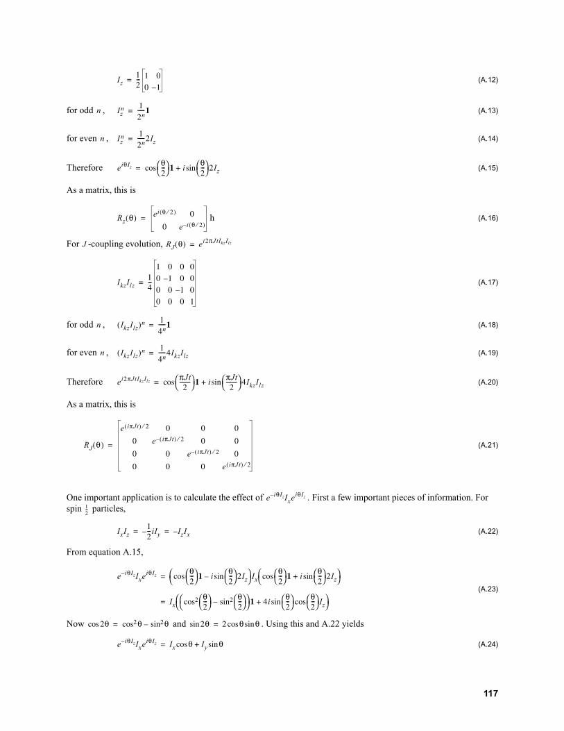
(A.12)
for odd , (A.13)
for even , (A.14)
Therefore (A.15)
As a matrix, this is
h (A.16)
For -coupling evolution,
(A.17)
for odd , (A.18)
for even , (A.19)
Therefore (A.20)
As a matrix, this is
(A.21)
One important application is to calculate the effect of . First a few important pieces of information. For spin particles,
(A.22)
From equation A.15,
(A.23)
Now and . Using this and A.22 yields
(A.24)
Iz
---
n Izn
n-----
n Izn
n-----Iz
eiθIzθ---
iθ---
Iz
Rz θ( ) ei θ ⁄( )
e i θ ⁄( )
J RJ θ( ) eiπJtIkzIlz
IkzIlz
---
n IkzIlz( )n
n-----
n IkzIlz( )n
n-----IkzIlz
eiπJtIkzIlzπJt
-------- i
πJt
-------- IkzIlz
RJ θ( )
e iπJt( ) ⁄
e iπJt( ) ⁄
e iπJt( ) ⁄
e iπJt( ) ⁄
e i θIzIxeiθIz
---
IxIz
--- iIy IzIx
e i θIzIxeiθIzθ---
iθ---
Iz Ix
θ---
iθ---
Iz
Ixθ---
θ---
iθ---
θ---
Iz
θ θ θ θ θ θ
e iθIz IxeiθIz Ix θ Iy θ
117
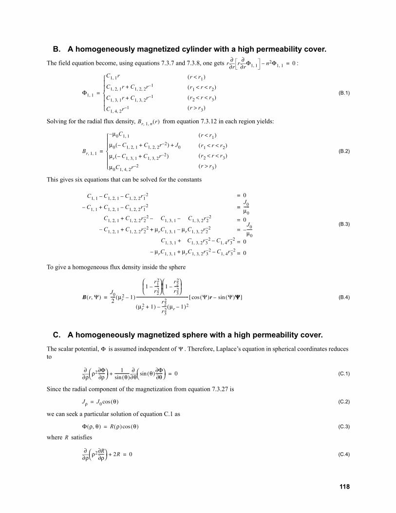
B. A homogeneously magnetized cylinder with a high permeability cover.
The field equation become, using equations 7.3.7 and 7.3.8, one gets :
(B.1)
Solving for the radial flux density, from equation 7.3.12 in each region yields:
(B.2)
This gives six equations that can be solved for the constants
(B.3)
To give a homogeneous flux density inside the sphere
(B.4)
C. A homogeneously magnetized sphere with a high permeability cover.
The scalar potential, is assumed independent of . Therefore, Laplace’s equation in spherical coordinates reduces to
(C.1)
Since the radial component of the magnetization from equation 7.3.27 is
(C.2)
we can seek a particular solution of equation C.1 as
(C.3)
where satisfies
(C.4)
rr∂
∂r
r∂∂ Φ , nΦ ,
Φ ,
C , r
C , , r C , , r
C , , r C , , r
C , , r
r r<( )
r r r< <( )
r r r< <( )
r r>( )
Br n, , r( )
Br , ,
µC ,
µ C , , C , , r ( ) J
µr C , , C , , r ( )
µC , , r
r r<( )
r r r< <( )
r r r< <( )
r r>( )
C , C , , C , , r
C , C , , C , , r
C , , C , , r C , , C , , r
C , , C , , r µrC , , µrC , , r
C , , C , , r C , r
µrC , , µrC , , r C , r
Jµ
------
Jµ
------
B r Ψ,( )J----- µr
( )
r
r
-----
r
r
-----
µr ( )
r
r
----- µr ( )
------------------------------------------------------ Ψ( ) r Ψ( ) ΨΨΨΨ[ ]
Φ Ψ
ρ∂∂ ρ Φ∂
ρ∂-------
θ( )---------------
θ∂∂
θ( )Φ∂θ∂
-------
Jρ J θ( )
Φ ρ θ,( ) R ρ( ) θ( )
R
ρ∂∂ ρ R∂
ρ∂------
R
118

The general solution is
(C.5)
Thus the scalar potential in each region becomes
(C.6)
and the radial component of the magnetic flux density becomes
(C.7)
These six equation can be solved for the constants
(C.8)
To give a homogeneous flux density inside the sphere
(C.9)
D. Homogeneous Field Solution for a Halbach Sphere
One would hope for a high flux density inside the sphere with no surrounding high permeable material if
(D.1)
The divergence of the remanence from above is
(D.2)
Thus Poisson’s equation in the region is
(D.3)
R ρ( ) Cρ Cρ
Φ
C , ρ
C , , ρ C , , ρ
C , , ρ C , , ρ
C , , ρ
ρ ρ<( )
ρ ρ ρ< <( )
ρ ρ ρ< <( )
ρ ρ>( )
Br
µC ,
µ C , , C , , ρ ( ) J
µr C , , C , , ρ ( )
µC , , ρ
ρ ρ<( )
ρ ρ ρ< <( )
ρ ρ ρ< <( )
ρ ρ>( )
C , C , , C , , ρ
C , C , , C , , ρ
C , , C , , ρ C , , C , , ρ
C , , C , , ρ µrC , , µrC , , ρ
C , , C , , ρ C , ρ
µrC , , µrC , , ρ C , ρ
Jµ
------
Jµ
------
B ρ θ,( )J----- µr ( ) µr ( )
ρ
ρ------
ρ
ρ------
µr ( ) µr
---
ρ
ρ------ µr ( )
--------------------------------------------------------------------------- θ( )ρρρρ θ( )θθθθ[ ]
J ρ θ,( ) J θ( ) ρρρρ θ( ) θθθθ[ ]
J∇•
ρ θ( )----------------------
ρ∂∂ ρ θ( ) Jρ ρ θ,( )( ) θ∂
∂ ρ θ( ) Jθ ρ θ,( )( )
J θ( )
ρ-------------------------
ρ ρ ρ< <
ρ∂∂ ρ Φ∂
ρ∂-------
θ( )---------------
θ∂∂ θ( )
Φ∂θ∂
-------
ρJ θ( )
µ
-----------------------------
119

Since the homogeneous field solution was solved earlier, simply let be the particular solution and solve
(D.4)
Let , thus giving
(D.5)
This must be true for all , so and giving
(D.6)
Modifying previous results for the constants in each region gives
(D.7)
Solving for gives a magnetic flux density
(D.8)
Φp Γ ρ( )ρ θ( )
ρ Γ ρ( ) θ( ) Γ' ρ( ) θ( )[ ] ρ ρ∂∂ Γ ρ( ) θ( ) Γ' ρ( )ρ θ( )[ ]
θ( )---------------
θ∂∂ θ( ) Γ ρ( )ρ( )
ρJµ
------------ θ( )
ρΓ' ρ( ) ρΓ'' ρ( )ρJ
µ
------------
Γ' ρ( ) Eρα
Eρα Eαρα Jµ
--------
ρ α EJµ
---------
Φ Cρ Cρ Jµ---------ρ ρ ρ( )
C , C , , C , , ρ
C , C , , C , , ρ
C , , C , , ρ C , ρ
C , , C , , ρ C , ρ
Jµ
--------- ρ( )
Jµ
--------- ρ( )Jµ
---------
Jµ
--------- ρ( )
Jµ
--------- ρ( )Jµ
---------
C ,
B ρ θ,( )J
--------ρρ-----
θ( ) ρρρρ θ( ) θθθθ[ ]
120
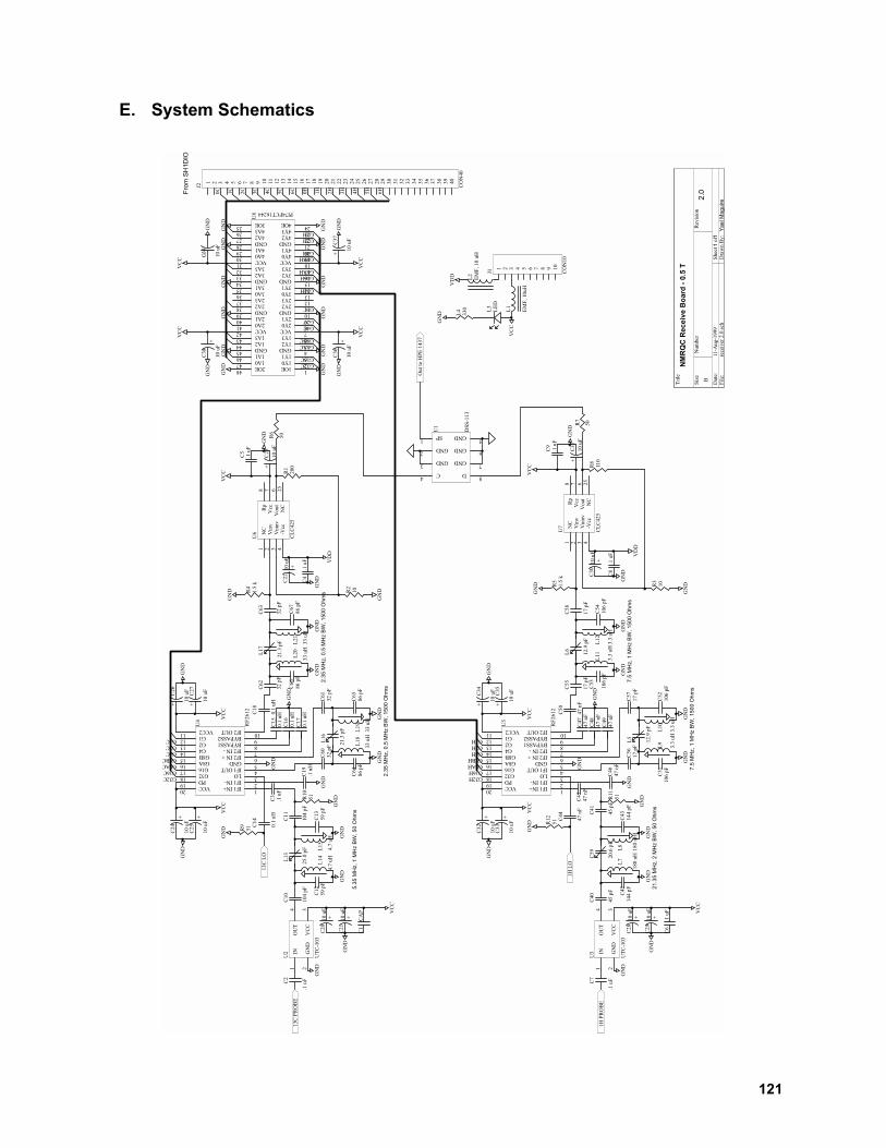
E. System Schematics
Tit
le
Num
ber
Revis
ion
Siz
e
B
Date
:11-A
ug-1
999
Sheet
o
f
Fil
e:
receiv
er
2.0
.sch
Dra
wn B
y:
13C
PR
OB
E
NM
RQ
C R
ecei
ve B
oar
d -
0.5
T
2.0
11
Yae
l Mag
uire
Out
to H
PE
1437
SP1
GND5
GND2
GND6
GND3
C4
GND7
D8
U1
DS
S-1
13
VC
C
GN
DG
ND
GN
D
GN
D
13C
LO
GN
D
IN1
OU
T4
GN
D2
VC
C3
U2
UT
C-1
03
IF1 IN+1
IF1 IN-2
LO3
IF1 OUT4
GND5
IF2 IN +6
IF2 IN -7
BYPASS18
BYPASS29
IF2 OUT10
VCC211
G112
G213
G414
G8B15
G8A16
G1617
G3218
PD19
VCC20
U4
RF
2612
GN
D
C1
CA
P
GN
D
C2
.1 u
F
C10
104 p
F
C12
59 p
F
C13
59 p
F
C14
0.1
uH
C11
104 p
F
C3
.1 u
F
C19
.1 u
H
C15
0.1
uH
C16
0.1
uH
C17
0.1
uH
+
C20
10 u
F
+
C21
10 u
F
NC
1
Vin
v2
Vnin
v3
-Vcc
4N
C25
Vout
6V
cc
7R
p8
U6
CL
C425
VD
D
C4
.1 u
F
+
C22
10 u
F
VC
C
C5
.1 u
F
+
C23
10 u
F
R1
200
R2
10
R4
1.5
k
R6
50
+
C24
10 u
F
+
C25
10 u
F
+
C26
10 u
F
+
C27
10 u
F
G16C
G8AC
G8BC
G4C
G2C
VC
CV
CC
GN
DG
ND
GN
D
GN
D
GN
D
GN
D
1H
PR
OB
E
GN
DG
ND
GN
D
GN
D GN
DG
ND
1H
LO
GN
D
IN1
OU
T4
GN
D2
VC
C3
U3
UT
C-1
03
IF1 IN+1
IF1 IN-2
LO3
IF1 OUT4
GND5
IF2 IN +6
IF2 IN -7
BYPASS18
BYPASS29
IF2 OUT10
VCC211
G112
G213
G414
G8B15
G8A16
G1617
G3218
PD19
VCC20
U5
RF
2612
GN
D
C6
.1 u
F
GN
D
C7
.1 u
F
C40
45 p
F
C42
144 p
F
C43
144 p
F
C44
47 n
F
C41
45 p
F
C45
47 n
F
C46
47
nF
C51
106 p
F
C52
106 p
F
C47
47 n
F
C48
47 n
F
C49
47 n
F
+
C28
10 u
F
+
C29
10 u
F
NC
1
Vin
v2
Vnin
v3
-Vcc
4N
C25
Vout
6V
cc
7R
p8
U7
CL
C425
VD
D
C8
.1 u
F
+
C30
10 u
F
VC
C
C9
.1 u
F
+
C31
10 u
F
R8
110
R3
10
R5
1.5
k
R7
50
+
C32
10 u
F
+
C33
10 u
F
+
C34
10 u
F
+
C35
10 u
F
G16H
G8AH
G8BH
G4H
G2H
VC
CV
CC
GN
DG
ND
GN
D
GN
D
GN
D
VC
C
1OE1
1Y02
1Y13
GND4
1Y25
1Y36
VCC7
2Y08
2Y19
GND10
2Y211
2Y312
3Y013
3Y114
GND15
3Y216
3Y317
VCC18
4Y019
4Y120
GND21
4Y222
4Y323
4OE24
3OE25
4A326
4A227
GND28
4A129
4A030
VCC31
3A332
3A233
GND34
3A135
3A036
2A337
2A238
GND39
2A140
2A041
VCC42
1A343
1A244
GND45
1A146
1A047
2OE48
U8
PI74FCT16244
GN
DG
ND
GN
DG
ND
GN
DG
ND
GN
DG
ND
GN
DG
ND
GN
DG
ND
VC
CV
CC
VC
CV
CC
G32C
G16C
G8AC
G8BC
G4C
G2C
G1C
G32H
G16H
G8AH
G8BH
G4H
G2H
G1H
G32C
+
C36
10
uF
+
C37
10
uF
+
C38
10
uF
+
C39
10 u
F
GN
DG
ND
GN
DG
ND
G1C G1H
G32H
Fro
m S
H1D
IO
C18
0.1
uH
C55
17 p
F
GN
D
GN
D
C53
106 p
F
C54
106 p
F
C56
17 p
F
C57
17 p
F
C58
17 p
F
GN
D
C50
47 n
F
GN
DG
ND
L1
EM
F, 10uH
L2
EM
F,
10
uH
VD
D
VC
C
L3
LE
D
L4
330
GN
D
1 2 3 4 5 6 7 8 9 10
J1 CO
N10
1 2 3 4 5 6 7 8 9 10
11
12
13
14
15
16
17
18
19
20
21
22
23
24
25
26
27
28
29
30
31
32
33
34
35
36
37
38
39
40
J2 CO
N40
0C
1C
2C
3C
4C
5C
6C
0H
1H
2H
3H
4H
5H
6H
R9
51
GN
D
R10
51
GN
D
L5
12.9
pF
C59
20.6
pF
R11
51
R12
51
GN
D
GN
D
L7
180 n
H
L8
180 n
H]
21.3
5 M
Hz,
2 M
Hz
BW
, 50
Ohm
sL
9
3.3
uH
L10
3.3
uH
7.5
MH
z, 1
MH
z B
W, 1
500
Ohm
s
7.5
MH
z, 1
MH
z B
W, 1
500
Ohm
s
L11
3.3
uH
L12
3.3
uH
L6
12.9
pF
L13
25.0
pF
L14
4.7
uH
L15
4.7
uH
GN
DG
ND
C60
32 p
F
C64
86
pF
C65
86 p
F
C61
32 p
F
L16
21.3
pF
L18
33 u
H
L19
33 u
H
C62
32 p
F
C66
86 p
F
C67
86 p
F
C63
32 p
F
L17
21.3
pF
L20
33 u
H
L21
33 u
H
5.35
MH
z, 1
MH
z B
W, 5
0 O
hms
2.35
MH
z, 0
.5 M
Hz
BW
, 150
0 O
hms
2.35
MH
z, 0
.5 M
Hz
BW
, 150
0 O
hms
121

Tit
le
Num
ber
Revis
ion
Siz
e
B
Date
:11-A
ug-1
999
Sheet
o
f
Fil
e:
transm
itte
r 2.0
.Sch
Dra
wn B
y:
HP
1445
HP
CW
GE
N1
HP
CW
GE
N 2
VE
E1
GN
D2
GN
D3
GN
D4
RF
25
GN
D6
GN
D7
GN
D8
RF
C9
GN
D10
GN
D11
RF
112
GN
D13
GN
D14
VC
C15
C1
16
U1
SW
-313
VE
E1
GN
D2
GN
D3
GN
D4
RF
25
GN
D6
GN
D7
GN
D8
RF
C9
GN
D10
GN
D11
RF
112
GN
D13
GN
D14
VC
C15
C1
16
U2
SW
-313
RF
1G
ND
2
IF3
IF4
GN
D5
GN
D7
GN
D6
LO
8
U3
SR
A-3
MH
RF
1G
ND
2
IF3
IF4
GN
D5
GN
D7
GN
D6
LO
8
U4
SR
A-3
MH
Puls
ed H
Puls
ed G
EN
2
GN
D
GN
D
GN
D
GN
D
GN
D
GN
D
GN
D
VC
C
VD
D
GN
D
GN
D
DIO
0
DIO
1G
ND
NM
RQ
C T
ran
smit
Bo
ard
- 0
.5 T
2.0
11
Yae
l Mag
uire
Out
to 1
H A
MP
CO
N1
CO
N2
CO
N1
CO
N3
CO
N6
CO
N5
CO
N4
CO
N7
SP1
GND5
GND2
GND6
GND3
C4
GND7
D8
U5
DS
S-1
13
RF IN1
VDD12
VDD23
VDD34
VDD45
VDD56
VDD67
VDD78
RF OUT9
G2010
G1011
GND12
GND13
G814
G415
G216
U6
RF
2420
GN
D
VC
C
C1
0.1
uF
C2
120 p
F
GN
D
GN
D
RF IN1
VDD12
VDD23
VDD34
VDD45
VDD56
VDD67
VDD78
RF OUT9
G2010
G1011
GND12
GND13
G814
G415
G216
U7
RF
2420
GN
D
GN
D
GN
D
C4
.1 u
F
C5
.1 u
F
VC
C
C3
120 p
F
C7
100 p
F
C8
100 p
F
C9
100 p
FC
10
100 p
F
C11
100 p
F
GN
D
GN
D
GN
D
GN
D
GN
D
C12
100 p
F
C13
100 p
F
C14
100 p
F
C15
100 p
F
C16
100 p
F
C6
.1 u
F
GN
D
GN
D
GN
DG
ND
C17
82 p
F
C19
144 p
F
C20
144 p
F
C18
82 p
F
C21
1.3
0 n
F
C23
2.7
0 n
FC
22
1.3
0 n
F
GN
DG
ND
GN
DG
ND
C24
0.1
uF
GN
DG
ND
C29
45 p
F
C31
243 p
F
C32
243 p
F
C30
45 p
F
GN
DG
ND
C33
72 p
F
C35
178 p
F
C36
178 p
F
C34
72 p
F
+C
37 10 u
F
+C
38
10 u
F
GN
D
+C
39
10 u
F+
C40
10 u
F
GN
D
+C
41 10 u
F
+C
42
10 u
F
VD
D
C25
0.1
uF
C26
0.1
uF
VC
C
+C
43
10 u
F+
C44
10 u
F
GN
D
C27
0.1
uF
C28
0.1
uF
+
C45
10 u
F
+
C54
CA
PA
CIT
OR
PO
L
IN1
OU
T2
3 4
U8
ER
A-3
C55
.1 u
F
C56
.1 u
F
Out
to 1
3C
AM
P
GN
D
GN
D
GN
D
GN
D
L1
10 u
H
R1
40
VC
C
IN1
OU
T2
3 4
U9
ER
A-3
+C
46
10 u
F+
C47
10 u
F
GN
D
L2
10 u
H
R2
40
VC
C
+C
48
10 u
F
+C
49
10
uF
GN
D
L3
EM
F, 10 u
H
VD
D
VC
C
L5
LE
D
L6
330
GN
D
1 2 3 4 5 6 7 8 9 10
J1 CO
N10
1OE1
1Y02
1Y13
GND4
1Y25
1Y36
VCC7
2Y08
2Y19
GND10
2Y211
2Y312
3Y013
3Y114
GND15
3Y216
3Y317
VCC18
4Y019
4Y120
GND21
4Y222
4Y323
4OE24
3OE25
4A326
4A227
GND28
4A129
4A030
VCC31
3A332
3A233
GND34
3A135
3A036
2A337
2A238
GND39
2A140
2A041
VCC42
1A343
1A244
GND45
1A146
1A047
2OE48
U10 PI74FCT16244
GN
DG
ND
GN
DG
ND
GN
DG
ND
GN
DG
ND
GN
DG
ND
GN
DG
ND
VC
CV
CC
VC
CV
CC
G20C
G10C
G8C
G4C
G2C
G20H
G10H
G8H
G4H
G2H
+
C50
10
uF
+
C51
10 u
F
+C
52
10
uF
+
C53
10 u
F
GN
DG
ND
GN
DG
ND
1 2 3 4 5 6 7 8 9 10
11
12
13
14
15
16
17
18
19
20
21
22
23
24
25
26
27
28
29
30
31
32
33
34
35
36
37
38
39
40
J2 CO
N40
G2H
G4H
G8H
G10H
G20H
GN
D
GN
D
GN
D
G20C
G10C
G8C
G4C
G2C
L4
EM
F, 10 u
H
0C
1C
2C
3C
4C
0H
1H
2H
3H
4H
GN
D
0H
1H
2H
3H
4H
0C
1C
2C
3C
4C
Fro
m S
H1D
IO
D0
D1
DIO0
DIO1
D0
D1
C57
120 p
F
C58
120 p
F
GN
D
GN
D
C59
27
.3 p
FL7
5.6
uH
L8
5.6
uH
L9
1.2
uH
L10
1.2
uH
C60
17.7
pF
L11
3.3
uH
L12
3.3
uH
L13
180 n
H
L14
180 n
H
C61
20.1
pF
5.35
MH
z, 1
MH
z B
W, 5
0 O
hms
21.3
5 M
Hz,
2 M
Hz
BW
, 50
Ohm
s
7.5
MH
z, 1
MH
z B
W, 5
0 O
hms
2.4
MH
z LP
F, 5
0 O
hms
122

Tit
le
Nu
mb
er
Revis
ion
Siz
e
B
Date
:10-A
ug-1
999
Sheet
o
f
File:
G:\
pro
tel\
TX
RX
\sh1nm
r2.0
.sch
Dra
wn B
y:
12345678910
11
12
13
14
15
16
17
18
19
20
J1 20
PIN
GN
D
1
23
U1
AM
C7
4F
12
5
PIN
SW
1A
PIN
SW
2B
12345678910
11
12
13
14
15
16
17
18
19
20
21
22
23
24
25
26
J2 26
PIN
GN
D
E1
44
5A
1 2 3 4 5 6 7 8 9
10
11
12
13
14
15
16
17
18
19
20
21
22
23
24
25
26
27
28
29
30
31
32
33
34
35
36
37
38
39
40
J3 40
PIN
E1
43
7A
1 2 3 4 5 6 7 8 9
10
11
12
13
14
15
16
17
18
19
20
21
22
23
24
25
26
27
28
29
30
31
32
33
34
35
36
37
38
39
40
J4 40
PIN
BA
14
45
BA
14
37
BA
1
BA
2
BA
4
BA
5
BB
1
BA
3
BB
2
BB
3
BB
4
BB
5
BC
1
HS
W
CS
W
BC
2
BC
3
BC
4
BC
5
BD
1
TT
L2
TT
L1
BD
2
BD
3
BD
4
BD
5
TT
L1
TT
L2
GN
D
GN
D
GN
D
GN
D
GN
D
HS
W
CS
W
BA
1
BA
2
HS
WC
HS
WC
CS
WC
CS
WC
CB
A1
CB
A1
GN
D
BA
3
BA
4
BA
5
BB
1
GN
D
BB
2
BB
3
BB
4
BB
5
GN
D
GN
D
PIN
SW
2A
PIN
SW
1B
GN
D
GN
D
GN
D
TT
L2
TT
L1
GN
D
GN
D
4
56
U1
BM
C7
4F
12
5
10
98
U1
CM
C7
4F
12
5
13
12
11
U1
DM
C7
4F
12
5
TT
L1A
TT
L2A
TT
L1
B
TT
L2
B
TT
L1A
TT
L2A
TT
L1
B
TT
L2
B
1
23
U2
A
MC
74
F1
25
4
56
U2
B
MC
74
F1
25
BA
14
45
BA
14
37
GN
D
GN
D
GN
D
GN
D
GN
D
GN
D
BA
14
45
C
BA
14
37
C
BA
14
45
C
BA
14
37
C
VC
C
VC
C
VC
C
VC
C
GN
D
GN
D
GN
D
GN
D
GN
D
GN
D
BC
1
BC
2
BC
3
BC
4
BC
5
BD
1
BD
2
BD
3
BD
4
BD
5
GN
D
GN
D
CB
C1
CB
C2
CB
C3
CB
C4
CB
C5
CB
D1
CB
D2
CB
D3
CB
D4
CB
D5
GN
D
GN
D
CB
C1
CB
C2
CB
C3
CB
C4
CB
C5
CB
D1
CB
D2
CB
D3
CB
D4
CB
D5
CB
A2
CB
A3
CB
A4
CB
A5
CB
B1
CB
B2
CB
B3
CB
B4
CB
B5
CB
A2
CB
A3
CB
A4
CB
A5
CB
B1
CB
B2
CB
B3
CB
B4
CB
B5
123456789
10
J5 CO
N1
0
VC
C
1 2 3 4 5 6
78910
J6 EZ
A-S
T
1 2 3 4 5 6
78910
J7 EZ
A-S
T
1 2 3 4 5 6
78910
J9 EZ
A-S
T
1 2 3 4 5 6
78910
J10
EZ
A-S
T
1 2 3 4 5 6
78910
J11
EZ
A-S
T
1 2 3 4 5 6
78910
J12
EZ
A-S
T
1 2 3 4 5 6
78910
J13
EZ
A-S
T
1 2 3 4 5 6
78910
J8 EZ
A-S
T
GN
D
Yae
l Mag
uire
SH
1 to
NM
R d
igit
al in
terf
ace
2.0
123
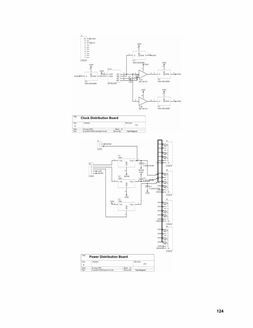
Title
Number RevisionSize
B
Date: 10-Aug-1999 Sheet of
File: G:\protel\TXRX\clockdist1.0.sch Drawn By:
CLR2
CKA1
QA3
QB4
QC5
QD6
U1A
SN74LS393
1
2 3
U2A
MC74F125
4
5 6
U2B
MC74F125
S1
GN
D2
GND3
U3
SMA HEADER
GND
GND
GND
U7
10KU8
10 K
GND
GND
S1
GN
D2
GND3
U4
SMA HEADER
S1
GN
D2
GND3
U5
SMA HEADER
S1
GN
D2
GND3
U6
SMA HEADER
GND
GND
GND
GND
GND
GND
GND
GND
1
2
3
4
5
6
7
8
9
10
J1
CON10
GND
VCC
Yael Maguire
Clock Distribution Board
1.0
Title
Number RevisionSize
B
Date: 10-Aug-1999 Sheet of
File: G:\protel\TXRX\power1.0.sch Drawn By:
Vin1
GN
D2
Vout3
U1
7805
1
2
J1
CON2
1
2
3
4
5J2
CON5
Vin1
GN
D2
Vout3
U2
7805
Vin1
GN
D2
Vout3
U3
7905
1
2
3
4
5
6
7
8
9
10
J3
CON10
GND
GND
GND
DGND
GND
GND
GND
GND
DGND
GND
C1
CAPACITOR
C2
CAPACITOR
C3
CAPACITOR
DGND
GND
GND
DGND
1
2
3
4
5
6
7
8
9
10
J4
CON10
1
2
3
4
5
6
7
8
9
10
J5
CON10
1
2
3
4
5
6
7
8
9
10
J6
CON10
GND
GND
GND
GND
DGND
GND
GND
GND
GND
GND
DGND
GND
GND
GND
GND
GND
DGND
GND
D5V
A5V
A-5V
D5V
D5V
D5V
D5V
A5V
A5V
A5V
A5V
A-5V
A-5V
A-5V
A-5V
DGND
Yael Maguire
Power Distribution Board
2.0
124

F. Hitachi Pulse Programmer Code
Cache.c contains the code my_main that will run inside the processor at full speed.
/* Cache.c. * E. Boyden. & Y. Maguire* (c) MIT Media Lab 1998 *//* PORTS * /#define PADR (*(volatile short int *)(0x5ffffc0))#define PBDR (*(volatile short int *)(0x5ffffc2))#define PAIOR (*(volatile short int *)(0x5ffffc4))#define PBIOR (*(volatile short int *)(0x5ffffc6))#define PACR1 (*(volatile short int *)(0x5ffffc8))#define PACR2 (*(volatile short int *)(0x5ffffca))#define PBCR1 (*(volatile short int *)(0x5ffffcc))#define PBCR2 (*(volatile short int *)(0x5ffffce))#define delay_cycles(x) (int __i; for (__i=0; __i < (x) ; __i++);)#define PIN_GATE 0xE100 /*pin J5-20,19,18,13; port PA15,14,13,8 1110 0001 0000 0000 */#define ATTEN1_PINS 0x2CDF /*pin J4-14,12,11,8-1;portPB13,11,10,7-0 0010 1100 1101 1111*/#define ATTEN2_PINSJ4 0x0020 /* pin J4-6; port PB5. 0000 0000 0010 0000 */#define ATTEN2_PINSJ5 0x1E8F /* J5-17,16,15,14,12,8-5; PA12,11,10,9,7,3,2,1,0 ->0001 1110 1000 1111*/#define TRIG_1445 0x8000 /* on port B, 15*/#define TRIG_1437 0x4000 /* PB14 */#define LED 0x8000 /*PB15 - same as 1445 trigger. */#define PBCR1_INIT 0x030F /* 0000 0011 0000 1111 */#define PBCR2_INIT 0x0000 /* 0000 0000 0000 0000 */#define PACR1_INIT 0x0000 /* 0 */#define PACR2_INIT 0x3F00 /* 0011 1111 0000 0000 */#define OUTPUTA_STUFF (PIN_GATE | ATTEN2_PINSJ5 )#define OUTPUTB_STUFF (ATTEN1_PINS | ATTEN2_PINSJ4 | TRIG_1445 | TRIG_1437 | LED)#define VECTORLENGTH 200long T[VECTORLENGTH]; /* transition times */short int R[VECTORLENGTH];/* pin-gate values */#define INST 100000int my_main()
short int i=0,j=0, loop=1, initloop=1, length = 0;short int attenuator1,attenuator2,__a,__b;char temp[11];SCI_init();SCIputs("Pulse Programmer 2.0 08/98\n\r");PBIOR |= OUTPUTB_STUFF; /* all output */PBCR1 &= PBCR1_INIT; /* 0101010101010101 --> turn off reserved/timing output */PBCR2 &= PBCR2_INIT; /* 0101010101010101 --> really does nothing */PAIOR |= OUTPUTA_STUFF; /* all output */PACR1 &= PACR1_INIT;PACR2 &= PACR2_INIT;PBDR &= ~(TRIG_1445 | TRIG_1437);/*Command hierarchycommands are:- 1 - start pulse sequence- 2 - attenuator data for TX board- 3 - attenuator data for RX board- 4 - pulse program data */while(initloop) PBDR &= ~(TRIG_1445 | TRIG_1437);SCIputs("Command?\n\r");SCIgets(temp);i = atoi(temp);switch(i) case 1 :
SCIputs("Starting step 1...\n\r");initloop = 0;break;
case 2 :
125

SCIputs("Enter bits 1-10.\n\r");SCIgets(temp);temp[5]='\0'; /* this depends on carriage returns */attenuator1 = atoi(temp);PBDR &= (~ATTEN1_PINS | attenuator1);PBDR |= (ATTEN1_PINS & attenuator1);break;
case 3 :SCIputs("Enter bits 11-20.\n\r");SCIgets(temp);temp[5]='\0';attenuator2 = atoi(temp);PADR &= (~ATTEN2_PINSJ5 | attenuator2);PADR |= (ATTEN2_PINSJ5 & attenuator2);PBDR &= (~ATTEN2_PINSJ4 | attenuator2);PBDR |= (ATTEN2_PINSJ4 & attenuator2);break;
case 4 :SCIputs("Enter length (up to 400)\n\r");SCIgets(temp);temp[5]='\0';SCIputs("Reading "); SCIputs(temp);length = atoi(temp);SCIputs("Enter times and values.\n\r");for (i=0; i < length; i++)
SCIgets(temp);temp[10]='\0'; /* carriage returns */T[i] = atol(temp);SCIgets(temp);temp[5]='\0';R[i] = atoi(temp);
SCIputs("Press enter to start.\n\r");SCIgets(temp);temp[10]='\0';PBDR |= TRIG_1445;for(__a=0;__a<length;__a++) __b = PADR;PADR = (__b | (PIN_GATE & R[__a])) & (~PIN_GATE | R[__a]);__b = PADR;int __bb;for(__bb=0;__bb<T[__a];__bb++);
PBDR |= TRIG_1437;break;
case 5:PBDR |= TRIG_1445;for(__a=0;__a<length;__a++) __b = PADR;PADR = (__b | (PIN_GATE & R[__a])) & (~PIN_GATE | R[__a]);__b = PADR;int __bb;for(__bb=0;__bb<T[__a];__bb++);
PBDR |= TRIG_1437;delay_cycles(100000); /* one led's worth */break;
default:SCIputs("[Unrecognized command]\n\r");break;
126
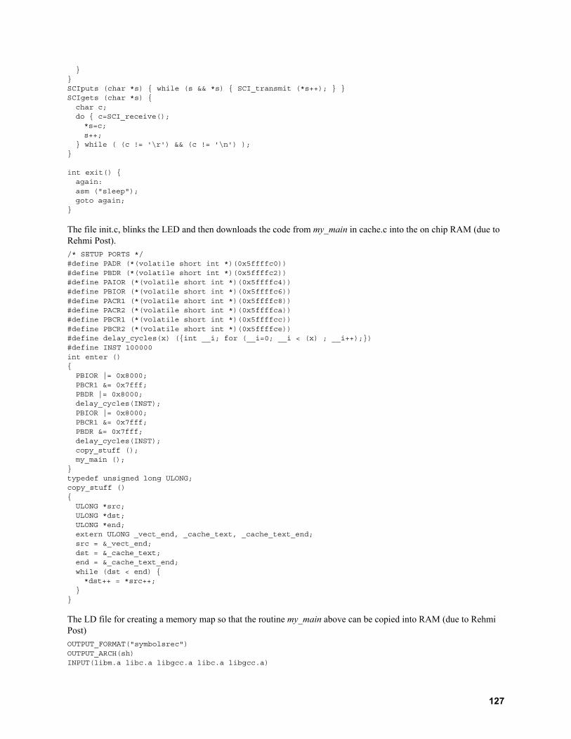
SCIputs (char *s) while (s && *s) SCI_transmit (*s++); SCIgets (char *s) char c;do c=SCI_receive();*s=c;s++;
while ( (c != '\r') && (c != '\n') );
int exit() again:asm ("sleep");goto again;
The file init.c, blinks the LED and then downloads the code from my_main in cache.c into the on chip RAM (due to Rehmi Post).
/* SETUP PORTS */#define PADR (*(volatile short int *)(0x5ffffc0))#define PBDR (*(volatile short int *)(0x5ffffc2))#define PAIOR (*(volatile short int *)(0x5ffffc4))#define PBIOR (*(volatile short int *)(0x5ffffc6))#define PACR1 (*(volatile short int *)(0x5ffffc8))#define PACR2 (*(volatile short int *)(0x5ffffca))#define PBCR1 (*(volatile short int *)(0x5ffffcc))#define PBCR2 (*(volatile short int *)(0x5ffffce))#define delay_cycles(x) (int __i; for (__i=0; __i < (x) ; __i++);)#define INST 100000int enter ()PBIOR |= 0x8000;PBCR1 &= 0x7fff;PBDR |= 0x8000;delay_cycles(INST);PBIOR |= 0x8000;PBCR1 &= 0x7fff;PBDR &= 0x7fff;delay_cycles(INST);copy_stuff ();my_main ();
typedef unsigned long ULONG;copy_stuff ()ULONG *src;ULONG *dst;ULONG *end;extern ULONG _vect_end, _cache_text, _cache_text_end;src = &_vect_end;dst = &_cache_text;end = &_cache_text_end;while (dst < end) *dst++ = *src++;
The LD file for creating a memory map so that the routine my_main above can be copied into RAM (due to Rehmi Post)
OUTPUT_FORMAT("symbolsrec")OUTPUT_ARCH(sh)INPUT(libm.a libc.a libgcc.a libc.a libgcc.a)
127

MEMORYrom : ORIGIN = 0x00000000, LENGTH = 64kram : ORIGIN = 0x0A000000, LENGTH = 128kcache : ORIGIN = 0x0F000000, LENGTH = 8k
SECTIONSvect_seg :*(.vect);
> rom__vect = ADDR(vect_seg);__vect_end = ADDR(vect_seg) + 1024;vrom_end = ((SIZEOF(vect_seg) + 1023) & ~ 1023);cache_text_seg : AT(vrom_end)cache.o(.text);
> cache__cache_text = ABSOLUTE(ADDR(cache_text_seg));__cache_text_end = ((ABSOLUTE(ADDR(cache_text_seg)) + SIZEOF(cache_text_seg) + 255) & ~ (255));ctext_end = vrom_end + ((SIZEOF(cache_text_seg) + 255) & ~ 255);rom_text_seg ctext_end : AT(ctext_end)CREATE_OBJECT_SYMBOLS;*(.init);*(.text);*(.strings);
> rom__rom_text = ABSOLUTE(ADDR(rom_text_seg));__rom_text_end = ((ABSOLUTE(ADDR(rom_text_seg)) + SIZEOF(rom_text_seg) + 255) & ~ (255));rtext_end = ctext_end + ((SIZEOF(rom_text_seg) + 255) & ~ 255);data_seg : AT(rtext_end)*(.data);
> cache__data = ABSOLUTE(ADDR(data_seg));__data_end = ((ABSOLUTE(ADDR(data_seg)) + SIZEOF(data_seg) + 255) & ~ (255));data_end = rtext_end + ((SIZEOF(data_seg) + 255) & ~ 255);uninit_data_seg : AT(data_end)*(.bss);*(COMMON);_end = . ;
> cache__uninit_data = ABSOLUTE(ADDR(uninit_data_seg));__uninit_data_end = ABSOLUTE(ADDR(uninit_data_seg)) + SIZEOF(uninit_data_seg);stack_seg 0x0F001ff4:*(.stack);
> cache__stack = ADDR(stack_seg);
G. Controlling the Spectrometer over IP in Java
To control a device which uses C/C++ DLL’s over IP in Java, there are two essential Java 2.0 pieces required. The first is called the Java Native Interface, which allows a Java program to make native C/C++ calls. The second required piece is Remote Method Invocation (RMI), which allows one to call methods over a remote network as if they existed within your own program and/or machine. An excellent tutorial can be found at [SUN99]. To begin, define a Java class containing methods that will be called natively:
/*
128

* e1445.class - this program declares the native c functions to call and loads the DLL/library* Yael Maguire* (c) MIT Media Lab, July 1999*/
class e1445 public native int startArb(); public native int start(); public native int sineFreq(double freq,double amp); public native int close(); public native int cmd(String cmd); public native int cmdString(String cmd, String text); public native int timeOut(int time); public native void check(int status); static System.loadLibrary("e1445");
Next, one compiles the class file: javac e1445.java. Then, the command javah e1445 creates a standard C/C++ header file for the native code. The native code is as follows:
/** e1445.cpp Yael Maguire*(c) MIT Media Lab July 1999*/#define VC_EXTRALEAN
#include <jni.h>#include "hpe1445.h"#include "visa.h"#include <iostream.h>#include "e1445.h"#include <stdlib.h>#include <windows.h>
ViStatus status;ViSession od;char onstrDesc[] = "VXI0::80::INSTR";char message[256];
// ARB ModeJNIEXPORT void JNICALLJava_e1145_startArb(JNIEnv *env, jobject obj)
// Select 40 MHz oscillator, set marker out to the 40 MHz oscillatorJNIEXPORT jint JNICALLJava_e1445_start(JNIEnv *env, jobject obj) cout << "\n";//startupcout << "Starting 1445.\n";status = hpe1445_init(onstrDesc, VI_FALSE, VI_TRUE, &od);Java_e1445_check(env, obj, status);status = hpe1445_errorQueryDetect(od, VI_TRUE);Java_e1445_check(env, obj, status);cout << "Setting internal oscillator to 40 MHz\n";status += hpe1445_cmd(od,"SOUR:ROSC:SOUR INT2");//choose internal 2 oscillator *Java_e1445_check(env, obj, status);cout << "Setting frequency of subsystem 2 to max\n";//MAX, so freq is 40000000status += hpe1445_cmdString(od, "SOUR:FREQ2:FIX", "MAX", VI_FALSE);//set frequency to Max *Java_e1445_check(env, obj, status);status = hpe1445_cmdString(od,"OUTP:FILT:LPAS:FREQ", "10 MHZ", VI_TRUE); //Java_e1445_check(env, obj, status);
129

status = hpe1445_cmdString(od,"OUTP:FILT:LPAS:STAT", "ON", VI_TRUE); //Java_e1445_check(env, obj, status);//create marker outcout << "Starting 40 MHz marker out.\n";status = hpe1445_cmdString(od, "SOUR:MARK:FEED", "\"SOUR:ROSC\"", VI_TRUE); //This makes the marker BNC 40 Mhz...Java_e1445_check(env, obj, status);cout << "1445 startup complete.\n";cout.flush();return (jint) status;
JNIEXPORT jint JNICALL Java_e1445_close (JNIEnv *, jobject) status = hpe1445_close(od);return status;
JNIEXPORT jint JNICALL Java_e1445_sineFreq (JNIEnv *, jobject, jdouble freq, jdouble ampl) status = hpe1445_sinWave(od, (ViReal64) freq, (ViReal64) ampl, hpe1445_Z_50 , "MIN");return (jint) status;
JNIEXPORT jint JNICALL Java_e1445_cmd (JNIEnv *, jobject, jstring cmd) status = hpe1445_cmd(od,(char *) cmd);return status;
JNIEXPORT jint JNICALL Java_e1445_cmdString (JNIEnv *, jobject, jstring cmd, jstring text) status = hpe1445_cmdString(od, (char *) cmd, (char *) text, VI_TRUE);return status;
JNIEXPORT jint JNICALL Java_e1445_timeOut (JNIEnv *, jobject, jint time)status = hpe1445_timeOut(od,time);return status;
JNIEXPORT void JNICALLJava_e1445_check(JNIEnv *, jobject, jint status) ViInt32 err_code;ViChar err_message[256];
if(VI_SUCCESS > (ViStatus) status) hpe1445_dcl(od);// send a device clear if(hpe1445_INSTR_ERROR_DETECTED == (ViStatus) status) err_code = 1;while (err_code) // instrument error hpe1445_error_query( od, &err_code, err_message); // query the scope sprintf(message,"1445 Instrument Error : %ld, %s\n", err_code, err_message); // display the error cout << message;
else // driver error hpe1445_error_message( od, status, err_message);// query the instrument sprintf(message,"1445 Driver Error : %ld, %s\n", status, err_message); // display the error cout << message;
hpe1445_reset(od); // reset the instrument hpe1445_close(od);// close the instrument handle Sleep(2000);cout.flush();
130

exit(1); return;
The code was compiled using Microsoft Visual Studio 6.0 into a DLL called e1445.dll. Then, one creates the RMI server that exists on the machine connected to the VXI interface which calls the native methods of e1445.java:
//exec.java, Yael Maguire//(c) MIT Media Lab, July 1999
import java.rmi.*;import java.rmi.server.UnicastRemoteObject;import java.io.*;
//public class exec public class exec extends UnicastRemoteObject implements execIntfpublic e1445 thise1445 = new e1445();public exec () throws java.rmi.RemoteException super();public int start() throws RemoteException int Status;Status = thise1445.start();return (Status);
public int startArb() throws RemoteException int Status;Status = thise1445.startArb();return (Status);
public int sineFreq(double freq,double amp) throws RemoteException int Status;Status = thise1445.sineFreq(freq,amp);return (Status);
public int timeOut(int time) int Status;Status = thise1445.timeOut(time);return Status;
public int cmd(String cmdt) int status;status = thise1445.cmd(cmdt);return status;
public int cmdString(String cmdt, String text) int status;status = thise1445.cmdString(cmdt,text);return status;
public int close() throws RemoteException int status;status = thise1445.close();return status;
public void check(int status) throws RemoteException thise1445.check(status);return;
public static void main (String args[]) System.setSecurityManager(new RMISecurityManager()); try
exec MyExec = new exec();Naming.rebind("/exec",MyExec);
131
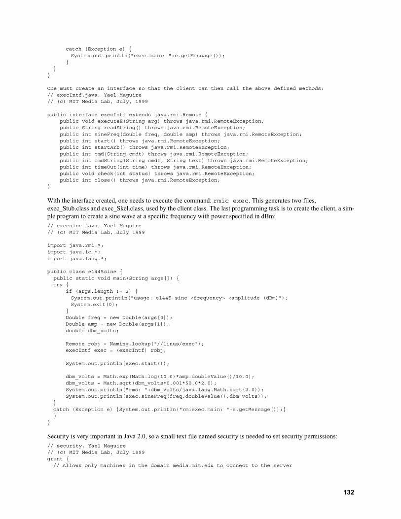
catch (Exception e) System.out.println("exec.main: "+e.getMessage());
One must create an interface so that the client can then call the above defined methods:// execIntf.java, Yael Maguire// (c) MIT Media Lab, July, 1999
public interface execIntf extends java.rmi.Remote public void executeE(String arg) throws java.rmi.RemoteException; public String readString() throws java.rmi.RemoteException; public int sineFreq(double freq, double amp) throws java.rmi.RemoteException; public int start() throws java.rmi.RemoteException; public int startArb() throws java.rmi.RemoteException; public int cmd(String cmdt) throws java.rmi.RemoteException; public int cmdString(String cmdt, String text) throws java.rmi.RemoteException; public int timeOut(int time) throws java.rmi.RemoteException; public void check(int status) throws java.rmi.RemoteException; public int close() throws java.rmi.RemoteException;
With the interface created, one needs to execute the command: rmic exec. This generates two files, exec_Stub.class and exec_Skel.class, used by the client class. The last programming task is to create the client, a sim-ple program to create a sine wave at a specific frequency with power specified in dBm:
// execsine.java, Yael Maguire// (c) MIT Media Lab, July 1999
import java.rmi.*;import java.io.*;import java.lang.*;
public class e1445sine public static void main(String args[]) try if (args.length != 2)
System.out.println("usage: e1445 sine <frequency> <amplitude (dBm)");System.exit(0);
Double freq = new Double(args[0]); Double amp = new Double(args[1]); double dbm_volts;
Remote robj = Naming.lookup("//linus/exec"); execIntf exec = (execIntf) robj; System.out.println(exec.start());
dbm_volts = Math.exp(Math.log(10.0)*amp.doubleValue()/10.0); dbm_volts = Math.sqrt(dbm_volts*0.001*50.0*2.0); System.out.println("rms: "+dbm_volts/java.lang.Math.sqrt(2.0)); System.out.println(exec.sineFreq(freq.doubleValue(),dbm_volts));catch (Exception e) System.out.println("rmiexec.main: "+e.getMessage());
Security is very important in Java 2.0, so a small text file named security is needed to set security permissions:
// security, Yael Maguire// (c) MIT Media Lab, July 1999grant // Allows only machines in the domain media.mit.edu to connect to the server
132
permission java.net.SocketPermission "*.media.mit.edu", "accept,connect";//Allow file permission to access DLL’spermission java.io.FilePermission "<<ALL FILES>>","read,execute";// Allow the runtime engine to load the e1445.dllpermission java.lang.RuntimePermission "loadLibrary.e1445";// Allow interaction with the system to obtain properties such as the name of the OS, etc.permission java.util.PropertyPermission "user.language","write";permission java.util.PropertyPermission "user.dir","read";
;
To start the server, first type “start rmiregistry” to run the rmi server. Then type “java -Djava.secu-rity.permission=security exec” to start the exec server. On the client, just type “java execsine 3000000 0” to get a 3 MHz, 0 dBm sine wave out of the HP E1445.
133

134
Bibliography
[ABE94] M. G. Abele. “Structures of Permanent Magnets - Generation of Uniform Fields.” New York: John Wiley and Sons Inc. 1993. pp. 1-67.
[AHA96a] D. Aharanov and M. Ben-Or. quant-ph/9611029.
[AHA96b] D. Aharanov and M. Ben-Or. quant-ph/9611025.
[ANA99] Analog Devices. http://www.analog.com
[ANS98] ANSYS 5.3 Technical documentation. 1998.
[ATC99] American Technical Ceramics. www.atceramics.com.
[AVA99] Avantek. http://www.em.avnet.com/rfm/mts/avantekdatasheets.html
[BAL91] Balian, Roger, D. Ter Haar. “From Microphysics to Macrophysics : Methods and Applications of Sta-
tistical Physics”. New York: Springer Verlag. 1992.
[BAR95a] Barenco et al. Phys Rev. A. 52., 3457. 1995.
[BAR95b] Barenco, Adriano. quant-ph/9505016.
[BAR96] A. Barenco et al. quant-ph/9601018.
[BEC96] David Beckman et al. quant-ph/9602016
[BEN82] Benioff, P. A. In. J. Theor. Phys. 21, 177 (182)
[BEN85] C. H. Bennett and R. Landauer, Scientific American, July, 1985, p. 48.
[BOW82] Bowick, Chris. “RF Circuit Design”. Carmel, IN: SAMS. 1982
[BOY96] Boyer, Michel et al. http://xxx.lanl.gov/quant-ph/9605034. 1996.
[BOY99] E. Boyden. Quantum Computation: Theory and Implementation. M. Eng Thesis. M.I.T. May, 1999.
[BRU99] Bruker. http://www.bruker.com/nmr/magnets/products/prodline/specprod.html.
[BUR99] Burkard, Guido, Daniel Loss and David P. DiVincenzo. Phys. Rev. B. 59. 3. 2070-2078. 1999
[CAL96] Calderbank, A. R. and P.W. Shor. Phys. Rev. A. 54. 1098. 1996.
[CER93] Cerny, V. Phys Rev A. 48. 116. 1993.
[CHM90] Chmruny, Gwendolyn N. and David I. Hoult. Concepts in Magnetic Resonance. 1990. 2, 131-149.
[CHO85] Cho, H. M et al. J. Chem Phys. 83, pp. 2775-2802. 1985.
[CHU88] T. E. Chupp et al. Phys. Rev. A. 38, 3998. 1998.
[CHU95] Chuang, I. et al. Science. 270, 1633. 1995.
135

[CHU98a] Isaac L. Chuang, Neil Gershenfeld, and Mark Kubinec. Physical Review Letters 80, pp. 3408-3411. 1998.
[CHU98b] I. L. Chuang et al. Proc. R. Soc. Lond. 454. pp. 447-467. (1998).
[CIR95] Cirac, J. I., and Zoller, P., Phys. Rev. Lett. 74. 4091. 1995.
[COP94] D. Coppersmith. IBM Research Report RC. 19642. 1994.
[COR97] Cory, D., Fahmy, A., Havel, T., Proc. Nat. Acad. Sci. 94. 1634. 1997.
[COR98] Cory, D. G. Price, M. D., Havel, T. F. Physica D. 120. 1-2. pp. 82-101. 1998.
[COR98b] Cory, D. G. et al. quant-ph/9802018.
[DEU85] Deutsch, D. Proc. R. Soc. London A. 400. 97. 1985.
[DEU89] Deutsch, D. Proc. R. Soc. London A. 425, 73 1989.
[DEU95] David Deutsch, Adriano Barenco, and Artur Ekert. quant-ph/950515.
[EKE96] A. Ekert and R. Jozsa. Rev. Mod. Phys. 68. 733. 1996.
[ERN87] Richard E. Ernst, G. Bodenhausen, and A. Wokaun. “Principles of Nuclear Magnetic Resonance in One and Two Dimensions.” Oxford: Clarendon Press. 1987
[FEY82] Feynman, R. P. Int. J. Theor. Phys. 21, 467. 1982.
[FLE97] Fletcher, R. R. “A Low-Cost Electromagnetic Tagging Technology for Wireless Identification, Sens-ing and Tracking of Objects.” Master’s Thesis MIT. 1997.
[FRE80] Ray Freeman, Stuart P. Kempsell and Malcolm Levitt. Journal of Magnetic Resonance. 38. 453-479. 1980.
[FRE82] E. Fredkin and T. Toffoli, Internat. J. Theoret. Phys. 21, 219. 1982.
[FRU98] Frutos, Anthony G. et al. “Enzymatic Ligation Reactions of DNA “Words” on Surfaces for DNA Computing''. J. Am. Chem. Soc., 120, 10277. 1998.
[FUK81] Fukushima, Eiichi et Stephen B. W. Roeder. “Experimental Pulse NMR: A Nuts and Bolts Approach”. Reading: Addison-Wesley Publishing Company. 1981.
[GER97] Neil A. Gershenfeld and Isaac L. Chuang. Science. 275. pp. 350-356. 1997.
[GER99a] N. Gershenfeld. “The Nature of Mathematical Modeling”. Cambridge: Cambridge University Press. 1999.
[GER99b] Gershenfeld,Neil, B. Schoner, and E. Metois. Nature 397, pp. 329-332 1999.
[GMW99] GMW Associates. www.gmw.com
[GOT98] Gottesman, D. Physical Review A, 57, No. 1, pp.127-37. January 1998.
[GRE98] S. A. Greenberg. Review of Modern Physics. 70, No. 1, pp. 175-222. January 1998.
[GRO97] Lov. K. Grover. Physical Review Letters. 79, pp. 325-328. 1997.
[GUE89] M. Guéron and J. L. Leroy. Journal of Magnetic Resonance. 85, 209-215. 1989.
[HAL85] Halbach, K. Proceedings of the Eight International Workshop on Rare Earth Cobalt Permanent Mag-nets and Their Applications. Dayton, Ohio. May 5-9, 1985, p. 103.
136
[HAY96] Hayward, Wes. “Introduction to Radio Frequency Design”. Beaverton, OR: The American Radio Relay League. 1996.
[HEW99a] Notes on PIN diode fundamentals for switching applications. http://ftp.hp.com/pub/accesshp/HP-COMP/rf/4_downld/lit/diodelit/an922.pdf
[HEW99b] Hewlett Packard. www.hp.com.
[HIT99] Hitachi Semiconductor 32-bit microcontrollers/microprocessors. http://semiconductor.hitachi.com/superh/?source=hitachi.com
[HIT99b] Hitachi NMR. www.hii.hitachi.com/r1200.htm.
[HOU76] Hoult, D. I. et R.E. Richards. Journal of Magnetic Resonance. 24, 71-85 (1976).
[HOU89] Hoult, D. I. et C-N Chen. “Biomedical Magnetic Resonance Technology”. Philadelphia: Institute of Physics Publishing. 1989.
[HUA87] Huang, Kerson. “Statistical Mechanics”. New York: John Wiley and Sons. 1987.
[HUS98] Hu, Sanlin et al. Rev. Sci. Instr. 69, No. 2., pp. 477-478. February 1998.
[INF99] Infotec. www.infotec.org/history.htm.
[JOZ97] Jozsa, Richard. quant-ph/9707034.
[KAN98] Kane B. E. Nature. 393, 6681. pp.133-7. 1998.
[KIR95] Kirsch J. et R. Newman. submitted to American Journal of Physics. http://web.mit.edu/8.13/JLExper-iments/JLExp_12AJP.pdf.
[KIT97] Kitaev, A. Yu. quant-ph/9707021.
[KLE81] Kleppner, D. Physical Review Letters. 47, p. 233 (1981)
[KNI97] Knill, E., Chuang, I., Laflamme, R. quant-ph/9706053.
[LEU98] Leung, Debbie et al. quant-ph/9811068.
[LEU99] Leung, Debbie. W. et al. quant-ph/9904100.
[LID98] Lidar, D. A., I. L . Chuang and K. B. Whaley. quant-ph/9807004.
[LIK91] Likharev K. and V. Semenov. IEEE Trans. on Appl. Supercond. 1, pp. 3-28, Mar. 1991.
[LLO93] Lloyd, Seth. Science. 261. 1569-71. 1993.
[LLO94] Llloyd, S. J. Mod. Opt. 41, 2503 (1994).
[LLO95] Lloyd, Seth. Physical Review Letters. 75. no. 2. 346. 1995.
[LOS98] Loss D, DiVincenzo DP. Physical Review A. 57, 1, 1998.
[MAC99] MA/COM. http://www.macom.com.
[MAR87] Margolis, Norman and Thomaso Toffoli. “Cellular automata machines : a new environment for mod-eling.” Cambridge, MA: MIT Press. 1987.
[MAT93] Mateescu, Gheorghe D. et Adrian Veleriu. “2D NMR Density Matrix and Product Operator Treat-ment”. New Jersey: Prentice Hall. 1993.
137

[MIC99] The PIN diode Handbook, version 2. Microsemi Corp. 1999. An online version exists at http://www.microsemi.com/micnotes/701.pdf
[MIN99] Mini-Circuits. http://www.minicircuits.com.
[MOO98] Moore, Gordon. www.intel.com/onedigitalday/explore/infinity/iessay.htm.
[MOO98c] Moore, Gordon. www.intel.com/intel/museum/25anniv/hof/moore.htm.
[MOT99] Motorola FM FSK Receivers for pager applications. http://mot-sps.com/cgi-bin/get?/books/dl110/pdf/mc3371rev*.pdf. Going to http://www.allied.avnet.com/cart/partdisplay.asp?PartNum-ber=8584565 will show the price to be $2.560 as of this writing.
[MRR99] MR Resources. http://www.mrr.com.
[NAT99] National Instruments. www.natinst.com.
[OXF99] Oxford Instruments. http://www.nmr.oxford-instruments.com/
[PAG81] Paget, D. Phys. Rev. B. vol.24, 7, 1, pp.3776-93. 1981.
[PER92] Peres, M. et al. Magnetic Resonance in Medicine. 27. 2 1992.
[PER93] Peres, Asher. “Quantum Theory: Concepts and Methods”. Kluwer Academic Publisher. 1993.
[POZ90] Pozar, David M. “Microwave Engineering.” Reading, MA: Addison-Wesley Publishing Company. 1990.
[PRE98] Preskill, J. Proc. Royal. Soc. Lon. A. 454, no. 1969. pp. 385-410. Jan. 1998.
[PRE93] Press, William H. et al. “Numerical Recipes in C, 2nd Ed.”. Cambridge: Cambridge Univeristy Press. 1993.
[RFM99] RF Microdevices. http://www.rfmd.com
[RLC88] RLC Resonator Book
[RSA99a] RSA Laboratories 476-bit challenge. http://www.rsa.com/rsalabs/html/twinkle.html
[RSA99b] RSA Laboratories. http://www.rsa.com.
[SAM99] S. Samaroo et al. Physical Review Letters. 82. pp. 5381-5384. 1999.
[SCH85] Schnall, M. D. et al. Journal of Magnetic Resonance. 65. 122-129. 1985.
[SCH98] Schmidt, JM. Molecular Physics. 95. no 5., 809-26. 1998.
[SHA99] Rütiger Shack and Carlton M. Caves. quant-ph/9903101.
[SHO95] Shor, Peter W. quant-ph/9508027.
[SHU98] Leonard J. Shulman and Umesh Vazirani. quant-ph/980460.
[SLE87] Sleator, Tycho et al. Physical Review B. 36, 4. pp. 1969-1980. 1987.
[SLI96] C. P. Slichter. “Principle of Magnetic Resonance”. New York: Springer-Verlag. 1996.
[STE96] Steane, A. Proc. Royal. Soc. London A. 452, 25551. 1996.
[STE97] Steane, Andrew. quant-ph/9708022.
138

[STE88] Steiglitz, K. Performance Limits in Communication Theory and Practice. Proceedings of the NATO advanced Study Institute. Klewer Academic Publishers. pp. 173-192. 1988.
[SUN87] Sunder Rajan, S., Wehrle, Janna P., and Jerry D. Glickson. Journal of Magnetic Resonance. 74. 147-154. 1987.
[SUN99] Sun’s Java tutorial and documentation site. http://java.sun.com/docs/index.html
[TEA99] Teachspin. http://www.teachspin.com
[TER43] F. E. Terman, “Radio Engineer’s Handbook”. New York: McGraw-Hill. 1st Ed. pp. 77-85. 1943.
[UNR95] Unruh, W. G. Phys. Rev. A. 51, 992. 1995.
[VAN99] Vandersypen, Lieven M. K., Yannoni, Constantino, Sherwood, Mark H, Chuang. I. L. quant-ph/9905041.
[VER86] A. Vergis, K. Steiglitz and B. Dickinson. Math. Comput. Simulation, 28. pp. 91-113. 1986.
[VOL99] Voltronics Corporation. http://www.voltronicscorp.com.
[WAR97] Warren S. Warren. Science. 277. pp. 1688-1689. 1997.
[WEB72] Webb, G. A. Annual Reports on NMR Spectroscopy. 5A. (1972), 10B. (1980).
[WOL86] Wolfram, Stephen. “Theory and applications of cellular automata : including selected papers 1983-1986.” Philadelphia: World Scientific. 1986.
[YAN99] Canstantino S. Yannoni et al. quant-ph/9907063.
[ZAL97] Zalka, Christof. quant-ph/9711070.
[ZVE67] Anatol I. Zverev. “Handbook of Filter Synthesis.” New York: John Wiley and Sons. 1967.
139