adaptive control of a mems steering mirror for free-space laser...

Adaptive Control of a MEMS Steering Mirror for Free-spaceLaser Communications

Nestor O. Perez Arancibia, Neil Chen, Steve Gibson and Tsu-Chin Tsao

Mechanical and Aerospace EngineeringUniversity of California, Los Angeles 90095-1597

ABSTRACTThis paper presents an adaptive control scheme for laser-beam steering by a two-axis MEMS tilt mirror usedin current free-space optical communications systems. In the control scheme presented here, disturbances inthe laser beam are rejected by a high-performance linear time-invariant feedback controller augmented by theadaptive control loop, which determines control gains that are optimal for the current disturbance acting onthe laser beam. The variable-order adaptive control loop is based on an adaptive lattice filter that implicitlyidentifies the disturbance statistics from real-time sensor data. Experimental results are presented to demonstratethe effectiveness of the adaptive controller for rejecting multi-bandwidth jitter. These results demonstrate thatthe adaptive loop significantly extends the jitter-rejection bandwidth achieved by the feedback controller alone.

Keywords: Adaptive control, laser-beam steering, jitter, MEMS mirror, free-space laser communications

1. INTRODUCTIONThe developing technology of free-space laser communications demands precise pointing of laser beams and high-bandwidth rejection of disturbances produced by platform vibrations and atmospheric turbulence. Vibration-induced jitter typically is composed of one or more narrow bandwidths produced by vibration modes of thestructure supporting the optical system, while turbulence-induced jitter may be rather broadband.1, 2 Also,some fast steering mirrors have lightly damped elastic modes that produce beam jitter. This is the case with theMEMS mirror used to steer the beam in the research described here. These mirrors, which are used in currentfree-space optical communications systems, have a torsional vibration mode about each steering axis.

Because the disturbance characteristics often change with time, optimal performance of a beam steeringsystem requires an adaptive control system. Recent research on jitter control has produced adaptive controlmethods that employ least-mean-square (LMS)3 adaptive filtering and recursive least-squares (RLS) adaptivefiltering.4–6 The trade off is between a simpler algorithm (hence computational economy) with LMS versusfaster convergence and exact minimum-variance steady-state performance with RLS.

This paper employs a recursive least-squares lattice filter in the adaptive controller, and introduces a variable-order adaptive control scheme that exploits the order-recursive structure of the lattice filter. The capability tovary the order of the filter in the adaptive controller is important because optimal gains can be identified fasterfor lower-order filters while higher-order filters are required for optimal steady-state rejection of broadbanddisturbance. Thus, low filter orders can be used initially for fast adaptation without undesirable transientresponses, and the filter order can be increased incrementally to achieve optimal steady-state jitter rejection.

The experiment used for this paper is similar to that used for two previous papers by the authors,5, 6 exceptfor one significant addition. As in these previous papers, a second mirror is used to add jitter to the laser beam;however, in the experiment described here, the MEMS mirror used as the control actuator is mounted on ashaker that vibrates with multiple bandwidths. Thus, there are two jitter sources here, as opposed to one in theauthors’ previous papers.

Section 2 describes the experimental hardware and configuration. Section 3 describes the system identificationof the mirror dynamics and transfer functions require for control system design. Section 4 describes the designof the control system, which consists of a linear time-invariant (LTI) feedback control loop augmented by theadaptive control loop. Experimental results for an experiment with multiple jitter bandwidths are presented inSection 5.

E-mail: [email protected], [email protected], [email protected], [email protected]

Free-Space Laser Communications V, edited by David G. Voelz, Jennifer C. Ricklin, Proc. of SPIE Vol. 5892(SPIE, Bellingham, WA, 2005) · 0277-786X/05/$15 · doi: 10.1117/12.619586

Proc. of SPIE 589210-1

Downloaded From: http://journals.spiedigitallibrary.org/ on 03/09/2014 Terms of Use: http://spiedl.org/terms

2. DESCRIPTION OF THE EXPERIMENT

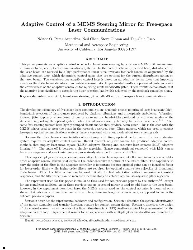
Fig. 1 shows a diagram of the experiment, including the path of the laser beam from the source to the positionsensor. The main optical components in the experiment are the laser source, two Texas Instruments MEMSfast steering mirrors, and an On-Trak position sensing device. These components are shown in the photographsin Figs. 2–refontrack. As indicated in Fig. 1, the laser beam leaves the fixed source and reflects first off themirror FSM 1, which serves as the control actuator. The beam then reflects off the mirror FSM 2, which addsdisturbance to the beam direction, and finally goes to the sensor. A lens between FSM 1 and FSM 2 and anotherlens between FSM 2 and the sensor focus the beam to maintain small spots on FSM 2 and the sensor. There aretwo sources of jitter in the experiment: the shaker on which the control actuator is mounted and the disturbanceactuator FSM 2. The motion of the shaker is vertical, and FSM 2 adds jitter on both mirror axes.

Each mirror rotates about vertical and horizontal axes, denoted by Axis 1 and Axis 2, respectively. Theoutputs of the sensor are the horizontal and vertical displacements of the centroid of the laser spot on the planeof the On-Track optical sensor. The sensor axes are labeled Axis 1 and Axis 2, respectively, to correspond tobeam deflections produced by the mirror rotations. Thus, in the sensor plane, Axis 1 and Axis 2 are horizontaland vertical, respectively.

FSM 1

FSM 2

Position SensingDevice

xPC Target SystemComputer 2

D\A

Laser BeamSource

Digital Control (DSP)Computer 1

A\DD\A5 6

1 2

3 4

Figure 1. Diagram of the UCLA beam steering experiment. MEMS mirror FSM 1: control actuator mounted on shaker;MEMS mirror FSM 2: disturbance actuator.

The output error in the control problem is the pair of sensor measurements, which are the coordinates of thelaser beam spot on the sensor. These measurements, in the form of voltages, go to Computer 1, which has aTexas Instruments TMS320C6701 digital signal processor. This DSP runs both feedback and adaptive controllersand sends actuator commands to FSM 1. Computer 2, a PC running xPC Target, sends disturbance commandsto FSM 2. It should be noted that the only measurements used by the adaptive and feedback controllers arethe two signals from the On-Trak sensor. The MEMS steering mirror used here has internal optical sensors thatsupply local measurements of the mirror position, but these measurements were not used in the experimentsdiscussed in this paper.

The commanded rotations of the fast steering mirrors are produced by electromagnetic fields with opposingdirections. These fields are created by coils with currents commanded by the control and disturbance computers.



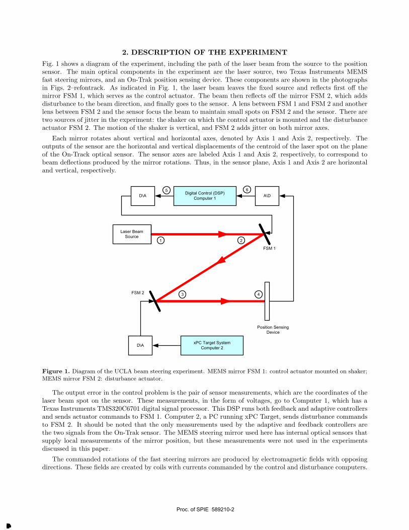
The mirrors have a rotation range of ±5 degrees. The reflecting area of the mirrors is 9mm2. The optoelectronicposition sensor at the end of the beam path generates two analog output voltages proportional to the two-dimensional position of the laser beam centroid. In the sensor, quad photo detectors capture the light intensitydistribution, generating current outputs, which are converted to voltage and amplified by an operational amplifier.Further electronic processing of these voltage signals yields two final signals, which are the estimates of thecentroid coordinates independent of light intensity.

Figure 2. The MEMS fast steering mirror FSM 1 is mounted on the shaker shown at left.

3.4 mm

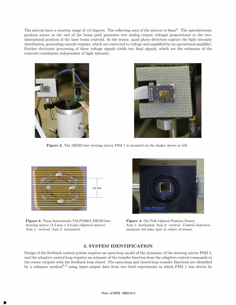
Figure 3. Texas Instruments TALP1000A MEMS faststeering mirror (3.2 mm × 3.6 mm elliptical mirror).Axis 1: vertical; Axis 2: horizontal.

Figure 4. On-Trak Optical Position Sensor.Axis 1: horizontal; Axis 2: vertical. Control objective:maintain red laser spot at center of sensor.

3. SYSTEM IDENTIFICATION

Design of the feedback control system requires an open-loop model of the dynamics of the steering mirror FSM 1,and the adaptive control loop requires an estimate of the transfer function from the adaptive-control commands tothe sensor outputs with the feedback loop closed. The open-loop and closed-loop transfer functions are identifiedby a subspace method7, 8 using input-output data from two brief experiments in which FSM 1 was driven by



white noise. After the first of these experiments, which was open-loop, the feedback controller was designed, andthen the feedback loop was closed for the second experiment.

Since the sample-and-hold rate for control and filtering was 2000Hz for the experimental results presented inthis paper, discrete-time models were identified for the 2000Hz rate. For identification, input-output sequenceswith 12,000 data points each (i.e., six seconds of data) were generated.

The disturbance actuator FSM 2 has dynamics very similar to those of FSM 1, but the control loops do notrequire a model of the disturbance actuator. Hence, the system identification uses data generated with FSM 2fixed.

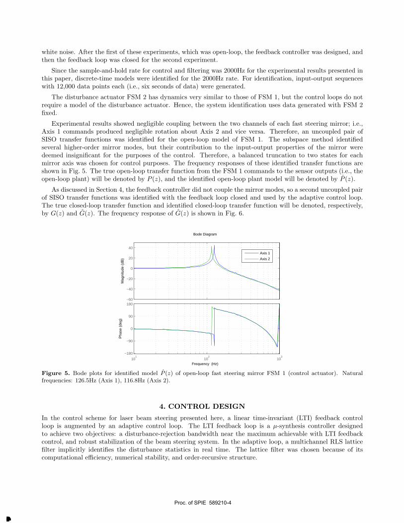
Experimental results showed negligible coupling between the two channels of each fast steering mirror; i.e.,Axis 1 commands produced negligible rotation about Axis 2 and vice versa. Therefore, an uncoupled pair ofSISO transfer functions was identified for the open-loop model of FSM 1. The subspace method identifiedseveral higher-order mirror modes, but their contribution to the input-output properties of the mirror weredeemed insignificant for the purposes of the control. Therefore, a balanced truncation to two states for eachmirror axis was chosen for control purposes. The frequency responses of these identified transfer functions areshown in Fig. 5. The true open-loop transfer function from the FSM 1 commands to the sensor outputs (i.e., theopen-loop plant) will be denoted by P (z), and the identified open-loop plant model will be denoted by P (z).

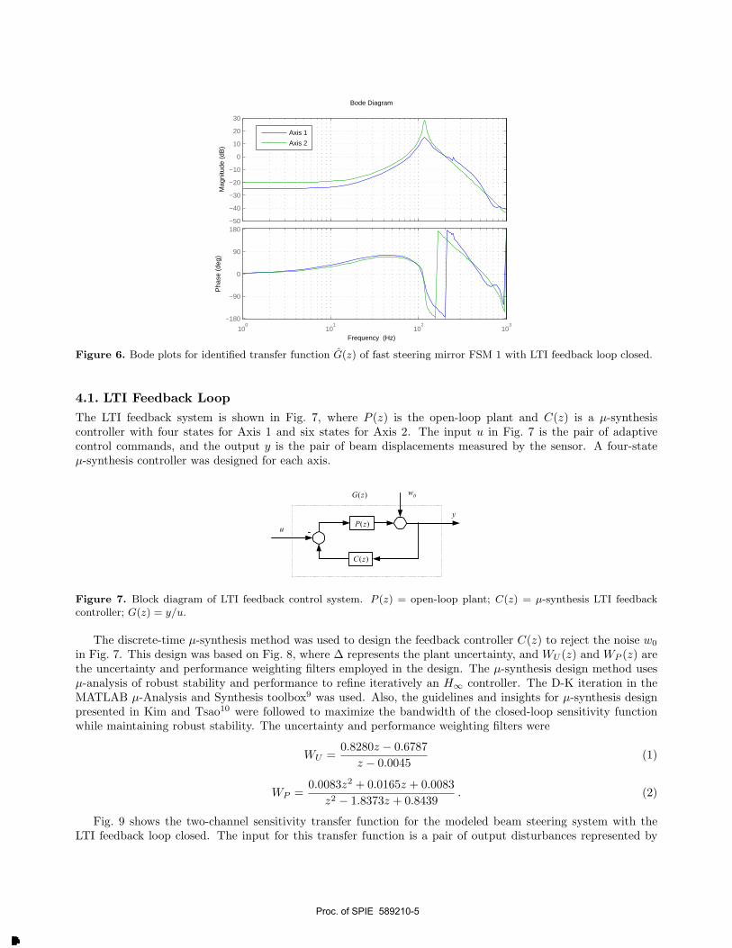
As discussed in Section 4, the feedback controller did not couple the mirror modes, so a second uncoupled pairof SISO transfer functions was identified with the feedback loop closed and used by the adaptive control loop.The true closed-loop transfer function and identified closed-loop transfer function will be denoted, respectively,by G(z) and G(z). The frequency response of G(z) is shown in Fig. 6.

−60

−40

−20

0

20

40

Mag

nitu

de (

dB)

101

102

103

−180

−90

0

90

180

Pha

se (

deg)

Bode Diagram

Frequency (Hz)

Axis 1

Axis 2

Figure 5. Bode plots for identified model P (z) of open-loop fast steering mirror FSM 1 (control actuator). Naturalfrequencies: 126.5Hz (Axis 1), 116.8Hz (Axis 2).

4. CONTROL DESIGN

In the control scheme for laser beam steering presented here, a linear time-invariant (LTI) feedback controlloop is augmented by an adaptive control loop. The LTI feedback loop is a µ-synthesis controller designedto achieve two objectives: a disturbance-rejection bandwidth near the maximum achievable with LTI feedbackcontrol, and robust stabilization of the beam steering system. In the adaptive loop, a multichannel RLS latticefilter implicitly identifies the disturbance statistics in real time. The lattice filter was chosen because of itscomputational efficiency, numerical stability, and order-recursive structure.



−50

−40

−30

−20

−10

0

10

20

30

Mag

nitu

de (

dB)

100

101

102

103

−180

−90

0

90

180

Pha

se (

deg)

Bode Diagram

Frequency (Hz)

Axis 1

Axis 2

Figure 6. Bode plots for identified transfer function G(z) of fast steering mirror FSM 1 with LTI feedback loop closed.

4.1. LTI Feedback LoopThe LTI feedback system is shown in Fig. 7, where P (z) is the open-loop plant and C(z) is a µ-synthesiscontroller with four states for Axis 1 and six states for Axis 2. The input u in Fig. 7 is the pair of adaptivecontrol commands, and the output y is the pair of beam displacements measured by the sensor. A four-stateµ-synthesis controller was designed for each axis.

)(zP

)(zG

)(zC

-u

y

w0

Figure 7. Block diagram of LTI feedback control system. P (z) = open-loop plant; C(z) = µ-synthesis LTI feedbackcontroller; G(z) = y/u.

The discrete-time µ-synthesis method was used to design the feedback controller C(z) to reject the noise w0

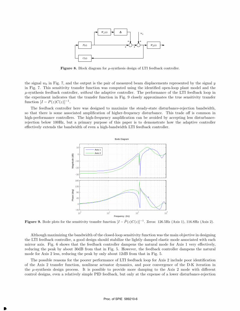
in Fig. 7. This design was based on Fig. 8, where ∆ represents the plant uncertainty, and WU (z) and WP (z) arethe uncertainty and performance weighting filters employed in the design. The µ-synthesis design method usesµ-analysis of robust stability and performance to refine iteratively an H∞ controller. The D-K iteration in theMATLAB µ-Analysis and Synthesis toolbox9 was used. Also, the guidelines and insights for µ-synthesis designpresented in Kim and Tsao10 were followed to maximize the bandwidth of the closed-loop sensitivity functionwhile maintaining robust stability. The uncertainty and performance weighting filters were

WU =0.8280z − 0.6787

z − 0.0045(1)

WP =0.0083z2 + 0.0165z + 0.0083

z2 − 1.8373z + 0.8439. (2)

Fig. 9 shows the two-channel sensitivity transfer function for the modeled beam steering system with theLTI feedback loop closed. The input for this transfer function is a pair of output disturbances represented by



P(z)

C(z)

WU(z)

WP(z)

w0

+

+ +

+

Figure 8. Block diagram for µ-synthesis design of LTI feedback controller.

the signal w0 in Fig. 7, and the output is the pair of measured beam displacements represented by the signal yin Fig. 7. This sensitivity transfer function was computed using the identified open-loop plant model and theµ-synthesis feedback controller, without the adaptive controller. The performance of the LTI feedback loop inthe experiment indicates that the transfer function in Fig. 9 closely approximates the true sensitivity transferfunction [I − P (z)C(z)]−1.

The feedback controller here was designed to maximize the steady-state disturbance-rejection bandwidth,so that there is some associated amplification of higher-frequency disturbance. This trade off is common inhigh-performance controllers. The high-frequency amplification can be avoided by accepting less disturbance-rejection below 100Hz, but a primary purpose of this paper is to demonstrate how the adaptive controllereffectively extends the bandwidth of even a high-bandwidth LTI feedback controller.

−30

−20

−10

0

10

Mag

nitu

de (

dB)

100

101

102

103

−45

0

45

90

135

180

Pha

se (

deg)

Bode Diagram

Frequency (Hz)

Axis 1

Axis 2

Figure 9. Bode plots for the sensitivity transfer function [I − P (z)C(z)]−1. Zeros: 126.5Hz (Axis 1), 116.8Hz (Axis 2).

Although maximizing the bandwidth of the closed-loop sensitivity function was the main objective in designingthe LTI feedback controller, a good design should stabilize the lightly damped elastic mode associated with eachmirror axis. Fig. 6 shows that the feedback controller dampens the natural mode for Axis 1 very effectively,reducing the peak by about 30dB from that in Fig. 5. However, the feedback controller dampens the naturalmode for Axis 2 less, reducing the peak by only about 12dB from that in Fig. 5.

The possible reasons for the poorer performance of LTI feedback loop for Axis 2 include poor identificationof the Axis 2 transfer function, nonlinear actuator dynamics, and poor convergence of the D-K iteration inthe µ-synthesis design process. It is possible to provide more damping to the Axis 2 mode with differentcontrol designs, even a relatively simple PID feedback, but only at the expense of a lower disturbance-rejection



bandwidth. However, the current feedback controller allows this paper to illustrate the performance of theadaptive loop when one axis is stabilized very well by the LTI feedback loop but one axis is not stabilized aswell.

4.2. Adaptive Control Loop

In typical beam-steering applications, including adaptive optics and optical wireless communications, the dynamicmodels of the fast steering mirrors either are known or can be determined by a one-time identification as inSection 3. The disturbance characteristics, however, depend on the atmospheric conditions in the optical pathsand on the excited vibration modes of the structures on which the optical systems are mounted, so that thedisturbance characteristics commonly vary during operation of a beam steering system. Therefore, the adaptivecontrol algorithm presented in this paper assumes known LTI plant dynamics but unknown disturbance dynamics.The adaptive controller requires an estimate G(z) of the closed-loop transfer function G(z) in Fig. 7. The RLSlattice filter in the adaptive control loop tracks the statistics of the disturbance and identifies gains to minimizethe RMS value of the beam displacement.

The adaptive control scheme used here is similar to the adaptive control schemes used in Kim et al.4 forexperimental adaptive control of a different type of fast steering mirror with much lower bandwidth than theMEMS mirror here, and in recent papers on adaptive optics11–14 where many sensor and control channels wereused but with lower filter orders than used here. The main control-scheme innovation in this paper is thevariable-order nature of the adaptive controller.

Fig. 10 shows the structure of the adaptive control loop. The disturbance signal w in Fig. 10 is related tothe disturbance signal w0 in Fig. 7 by the sensitivity transfer function produced by the LTI feedback loop (seeFig. 9):

w = [I − P (z)C(z)]−1w0 . (3)

The adaptive FIR filter F (z) is the main component of the adaptive controller. As shown in Fig. 10, theadaptive controller uses two copies of the FIR filter. The optimal filter gains are estimated in the bottom partof the block diagram in Fig. 10, and these gains are used by the FIR filter in the top part of Fig. 10 to generatethe adaptive control signal u..

For the results presented in this paper, the two channels of the adaptive controller were uncoupled, althoughthe adaptive lattice filter permits the use of multiple sensor channels for generating the command for each controlchannel. Comparison of a variety experimental results for the jitter-control system here showed that coupling thetwo channels in the adaptive controller produced no improvement in steady-state performance but the FIR gainsconverged faster to the optimal values for the uncoupled case because this case involves fewer FIR gains. Becauseof the multichannel nature of the lattice filter, the adaptive control algorithm can accommodate additional sensorsignals, such as accelerometer measurements.

The lattice structure of the FIR filter that generates the adaptive control commands is illustrated in Fig. 11.The lattice realization of an FIR filter of order N consists of N identical stages cascaded as in Fig. 11. The detailsof the lattice-filter algorithms represented by the blocks in Fig. 11 are beyond the scope of this paper. Thesealgorithms are reparameterized versions of algorithms in Jiang and Gibson.15 The current parameterization ofthe lattice algorithms is optimized for indefinite real-time operation. The current lattice filter maintains twoimportant characteristics of the RLS lattice filter in Jiang and Gibson15: channel orthogonalization, which isessential to numerical stability in multichannel applications, and the unwindowed property of the lattice filter,which is essential to rapid convergence.

As indicated in Fig. 11, each stage of the lattice filter generates an adaptive control command. For n ≥ 1, theoutput un from the nth stage is the optimal control command if an FIR filter of order n is used in the adaptivecontrol loop. For hardware implementation, a maximum filter order N is selected. In each real-time samplinginterval, the lattice filter generates the adaptive control commands for all filter orders from 1 to N, and thecontrol algorithm can select which command to use.



Closed Loop Plant

)(zG

Closed Loop Plant Model

)(ˆ zG

+

+

Copy of

)(zF

output

+

-

edisturbanc

u

Closed Loop Plant ModelLattice Filter)(zF )(ˆ zGz

1

z

1

Adaptive Lattice AlgorithmComputes Gains for

)(zF+ Error

m

w

w

yv

-

Figure 10. Block diagram of adaptive control system.

BackwardBlockn=1

z-1 z-1 z-1ForwardBlockn=1

ForwardBlockn=2

BackwardBlockn=2

BackwardBlockn=N

ForwardBlockn=N

1u 2u Nu

w

Figure 11. The FIR lattice filter generates adaptive control commands uk for all filter orders k ≤ N .

It should be emphasized that, because of the order-recursive structure of the lattice filter, computing thecontrol commands for all orders from 1 to N requires no more computation than computing the control commandfor the order N alone. It appears that lattice filters are the only RLS algorithms with this property. Therefore,lattice filters are uniquely suited to variable-order adaptive control.

The capability to vary the order of the filter in the adaptive controller is important because optimal gains canbe identified faster for lower-order filters while higher-order filters are required for optimal steady-state rejectionof broadband disturbance. When the adaptive control loop is first closed or when it is adapting to changing



disturbance statistics, lower-order control commands should be used initially. The order of the control commandscan be increased incrementally as the gains for the higher-order filter stages converge. This procedure eliminateslarge transient responses often produced by initially incorrect gains in high-order filters.

5. EXPERIMENTAL RESULTS

In the experiments described here, the sample-and-hold rate for control and filtering was 2000Hz. Computer2 in Fig. 1 sent jitter command sequences of multiple bandwidths to both the disturbance mirror FSM 2 andthe shaker. The same command sequence was sent to both axes of FSM 2. The command sequence sent to theshaker was the sum of the command sequence sent to FSM 2 and five sine waves (i.e., five discrete frequencies).These bandwidths and discrete frequencies were

jitter bandwidths for FSM 2 and shaker = 10Hz–20Hz, 190Hz–200Hz, 350–360Hz(4)

frequencies of sine waves for shaker = 15Hz, 40Hz, 125Hz, 195Hz, 355Hz.

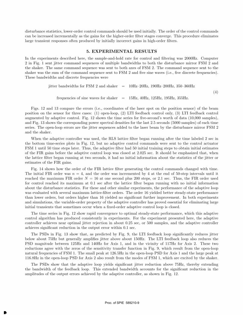
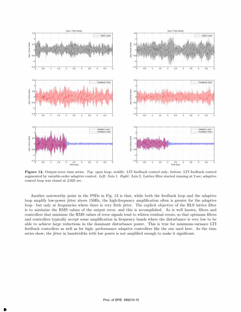
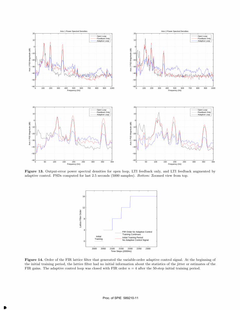
Figs. 12 and 13 compare the errors (i.e., coordinates of the laser spot on the position sensor) of the beamposition on the sensor for three cases: (1) open-loop, (2) LTI feedback control only, (3) LTI feedback controlaugmented by adaptive control. Fig. 12 shows the time series for five-second’s worth of data (10,000 samples),and Fig. 13 shows the corresponding power spectral densities for the last 2.5 seconds (5000 samples) of each timeseries. The open-loop errors are the jitter sequences added to the laser beam by the disturbance mirror FSM 2and the shaker.

When the adaptive controller was used, the RLS lattice filter began running after the time labeled 2 sec inthe bottom time-series plots in Fig. 12, but no adaptive control commands were sent to the control actuatorFSM 1 until 50 time steps later. Thus, the adaptive filter had 50 initial training steps to obtain initial estimatesof the FIR gains before the adaptive control loop was closed at 2.025 sec. It should be emphasized that, whenthe lattice filter began running at two seconds, it had no initial information about the statistics of the jitter orestimates of the FIR gains.

Fig. 14 shows how the order of the FIR lattice filter generating the control commands changed with time.The initial FIR order was n = 4, and the order was incremented by 4 at the end of 50-step intervals until itreached the maximum FIR order N = 16 at one second plus 200 steps, or 2.1 sec. Thus, the FIR order usedfor control reached its maximum at 0.1 sec after the lattice filter began running with no initial informationabout the disturbance statistics. For these and other similar experiments, the performance of the adaptive loopwas evaluated with several maximum lattice-filter orders. The order 16 yielded better steady-state performancethan lower orders, but orders higher than 16 yielded no significant further improvement. In both experimentsand simulations, the variable-order property of the adaptive controller has proved essential for eliminating largeinitial transients that sometimes occur when a fixed-order adaptive control loop is closed.

The time series in Fig. 12 show rapid convergence to optimal steady-state performance, which this adaptivecontrol algorithm has produced consistently in experiments. For the experiment presented here, the adaptivecontroller achieves near optimal jitter rejection in about 0.25 sec, or 500 samples, and the adaptive controllerachieves significant reduction in the output error within 0.1 sec.

The PSDs in Fig. 13 show that, as predicted by Fig. 9, the LTI feedback loop significantly reduces jitterbelow about 75Hz but generally amplifies jitter above about 150Hz. The LTI feedback loop also reduces thePSD magnitude between 125Hz and 140Hz for Axis 1, and in the vicinity of 117Hz for Axis 2. These tworeductions agree with the zeros of the sensitivity transfer function in Fig. 9, which result from the open-loopnatural frequencies of FSM 1. The small peak at 126.5Hz in the open-loop PSD for Axis 1 and the large peak at116.8Hz in the open-loop PSD for Axis 2 also result from the modes of FSM 1, which are excited by the shaker.

The PSDs show that the adaptive loop yields significant jitter reduction above 75Hz, thereby extendingthe bandwidth of the feedback loop. This extended bandwidth accounts for the significant reduction in theamplitudes of the output errors achieved by the adaptive controller, as shown in Fig. 12.



0 0.5 1 1.5 2 2.5 3 3.5 4 4.5 5−1.5

−1

−0.5

0

0.5

1

1.5

Axi

s 1

Err

or (

mm

)Axis 1 Time Series

Open Loop

0 0.5 1 1.5 2 2.5 3 3.5 4 4.5 5−1.5

−1

−0.5

0

0.5

1

1.5

Axi

s 1

Err

or (

mm

)

Feedback Only

0 0.5 1 1.5 2 2.5 3 3.5 4 4.5 5−1.5

−1

−0.5

0

0.5

1

1.5

Time (sec)

Axi

s 1

Err

or (

mm

)

Adaptive LoopFeedback Only

0 0.5 1 1.5 2 2.5 3 3.5 4 4.5 5−1.5

−1

−0.5

0

0.5

1

1.5

Axi

s 2

Err

or (

mm

)

Axis 2 Time Series

Open Loop

0 0.5 1 1.5 2 2.5 3 3.5 4 4.5 5−1.5

−1

−0.5

0

0.5

1

1.5

Axi

s 2

Err

or (

mm

)

Feedback Only

0 0.5 1 1.5 2 2.5 3 3.5 4 4.5 5−1.5

−1

−0.5

0

0.5

1

1.5

Time (sec)

Axi

s 2

Err

or (

mm

)Adaptive LoopFeedback Only

Figure 12. Output-error time series. Top: open loop; middle: LTI feedback control only; bottom: LTI feedback controlaugmented by variable-order adaptive control. Left: Axis 1. Right: Axis 2. Lattice filter started running at 2 sec; adaptivecontrol loop was closed at 2.025 sec.

Another noteworthy point in the PSDs in Fig. 13 is that, while both the feedback loop and the adaptiveloop amplify low-power jitter above 150Hz, the high-frequency amplification often is greater for the adaptiveloop—but only at frequencies where there is very little jitter. The explicit objective of the RLS lattice filteris to minimize the RMS values of the output error, and this is accomplished. As is well known, filters andcontrollers that minimize the RMS values of error signals tend to whiten residual errors, so that optimum filtersand controllers typically accept some amplification in frequency bands where the disturbance is very low to beable to achieve large reductions in the dominant disturbance power. This is true for minimum-variance LTIfeedback controllers as well as for high- performance adaptive controllers like the one used here. As the timeseries show, the jitter in bandwidths with low power is not amplified enough to make it significant.



0 100 200 300 400 500 600 700 800 900 1000−60

−50

−40

−30

−20

−10

0

10

20

Frequency (Hz)

Axi

s 1

PS

D M

agni

tude

(dB

)Axis 1 Power Spectral Densities

Open LoopFeedback OnlyAdaptive Loop

0 100 200 300 400 500 600 700 800 900 1000−60

−50

−40

−30

−20

−10

0

10

20

Frequency (Hz)

Axi

s 2

PS

D M

agni

tude

(dB

)

Axis 2 Power Spectral Densities


0 50 100 150 200 250 300 350 400−60

−50

−40

−30

−20

−10

0

10

20

Frequency (Hz)

Axi

s 1

PS

D M

agni

tude

(dB

)


0 50 100 150 200 250 300 350 400−60

−50

−40

−30

−20

−10

0

10

20

Frequency (Hz)

Axi

s 2

PS

D M

agni

tude

(dB

)


Figure 13. Output-error power spectral densities for open loop, LTI feedback only, and LTI feedback augmented byadaptive control. PSDs computed for last 2.5 seconds (5000 samples). Bottom: Zoomed view from top.

2000 2050 2100 2150 2200 2250 2300

0

4

8

12

16

Time Steps (2000Hz)

Latti

ce F

ilter

Ord

er

FIR Order for Adaptive ControlTraining Continues

Initial Training PeriodNo Adaptive Control Signal

InitialTraining

Figure 14. Order of the FIR lattice filter that generated the variable-order adaptive control signal. At the beginning ofthe initial training period, the lattice filter had no initial information about the statistics of the jitter or estimates of theFIR gains. The adaptive control loop was closed with FIR order n = 4 after the 50-step initial training period.



6. CONCLUSIONS

This paper has presented a new method for adaptive control of jitter in laser beams. The method has beendemonstrated by results from an experiment employing two-axis MEMS tilt mirrors. Laser beam jitter is rejectedby a µ-synthesis feedback controller augmented by a variable-order adaptive controller, which determines controlgains that are optimal for the current disturbance acting on the laser beam. The adaptive loop is based on an RLSlattice filter that implicitly identifies the disturbance statistics from real-time sensor data. Experimental resultsdemonstrate that the adaptive controller significantly extends the disturbance rejection bandwidth achieved bythe feedback controller alone. The adaptive lattice filter can perform high order, multi-channel RLS (recursive-least-squares) computation in real-time at high sampling rates, and the RLS algorithm yields faster convergenceto optimal gains than does the LMS method, which is used more commonly in adaptive disturbance-rejectionapplications. Even though a robust, high-performance feedback controller is used here, the experimental resultsdemonstrate that the adaptive controller greatly extends the jitter-rejection bandwidth.

ACKNOWLEDGMENTS

This work was supported by the U. S. Air Force Office of Scientific Research under AFOSR Grants F49620-02-01-0319 and F-49620-03-1-0234.

REFERENCES1. M. C. Roggemann and B. Welsh, Imaging through Turbulence, CRC, New York, 1996.2. R. K. Tyson, Principles of Adaptive Optics, Academic Press, New York, 1998.3. Mark A. McEver, Daniel G. Cole, and Robert L. Clark, “Adaptive feedback control of optical jitter using

Q-parameterization,” Optical Engineering , pp. 904–910, April 2004.4. Byung-Sub Kim, Steve Gibson, and Tsu-Chin Tsao, “Adaptive control of a tilt mirror for laser beam

steering,” in American Control Conference, IEEE, (Boston, MA), June 2004.5. Nestor O. Perez Arancibia, Steve Gibson, and Tsu-Chin Tsao, “Adaptive control of MEMS mirrors for beam

steering,” in IMECE2004, ASME, (Anaheim, CA), November 2004.6. Nestor O. Perez Arancibia, Neil Chen, Steve Gibson, and Tsu-Chin Tsao, “Adaptive control of a MEMS

steering mirror for suppression of laser beam jitter,” in American Control Conference, IEEE, (Portland,OR), June 2005.

7. Y. M. Ho, G. Xu, and T. Kailath, “Fast identification of state-space models via exploitation of displacementstructure,” IEEE Transactions on Automatic Control 39, pp. 2004–2017, October 1994.

8. P. Van Overschee and B. De Moor, Subspace Identification for Linear Systems, Kluwer Academic Publishers,Norwell, MA, 1996.

9. G. J. Balas, J. C. Doyle, K. Glover, A. Packard, and R. Smith, µ-Analisis and Synthesis Toolbox, Mathworks,1995.

10. B.-S. Kim and T.-C. Tsao, “A performance enhancement scheme for robust repetitive control system,”ASME Journal of Dynamic Systems, Measurement, and Control 126, pp. 224–229, March 2004.

11. J. S. Gibson, C.-C. Chang, and B. L. Ellerbroek, “Adaptive optics: wavefront correction by use of adaptivefiltering and control,” Applied Optics, Optical Technology and Biomedical Optics , pp. 2525–2538, June 2000.

12. J. S. Gibson, C.-C. Chang, and Neil Chen, “Adaptive optics with a new modal decomposition of actuatorand sensor spaces,” in American Control Conference, (Arlington, VA), June 2001.

13. Yu-Tai Liu and Steve Gibson, “Adaptive optics with adaptive filtering and control,” in American ControlConference, IEEE, (Boston, MA), June 2004.

14. Yu-Tai Liu, Neil Chen, and Steve Gibson, “Adaptive filtering and control for wavefront reconstruction andjitter control in adaptive optics,” in American Control Conference, IEEE, (Portland, OR), June 2005.

15. S.-B. Jiang and J. S. Gibson, “An unwindowed multichannel lattice filter with orthogonal channels,” IEEETransactions on Signal Processing 43, pp. 2831–2842, December 1995.



adaptive control of a mems steering mirror for free-space laser...

Documents