a new method for error modeling in the kinematic

A New Method for Error Modeling in the KinematicCalibration of Redundantly Actuated ParallelKinematic MachineLei-Ying He

Zhejiang Sci-Tech UniversityZhen-Dong Wang

Zhejiang Sci-Tech UniversityQin-Chuan Li ( [email protected] )

Zhejiang Sci-Tech UniversityXin-Xue Chai

Zhejiang Sci-Tech University

Original Article

Keywords: Error modeling, Redundant actuation, Sub-mechanism, Kinematic calibration

Posted Date: September 2nd, 2020

DOI: https://doi.org/10.21203/rs.3.rs-68445/v1

License: This work is licensed under a Creative Commons Attribution 4.0 International License. Read Full License

https://doi.org/10.21203/rs.3.rs-68445/v1

mailto:[email protected]

https://doi.org/10.21203/rs.3.rs-68445/v1

https://creativecommons.org/licenses/by/4.0/

A new method for error modeling in the kinematic calibration of redundantly actuated parallel kinematic machine ·1·

Title page

A new method for error modeling in the kinematic calibration of redundantly actuated parallel

kinematic machine

Lei-Ying He, born in 1983, is currently a Lecturer at Faculty of Mechanical Engineering & Automation, Zhejiang Sci-Tech University,

China. He received his PhD. degree from Zhejiang Sci-Tech University, China, in 2014. His research interests include kinematic calibration and robot vision. E-mail: [email protected] Zhen-Dong Wang, born in 1993, received his master degree in Zhejiang Sci-Tech University, China, in 2019. His research interest is the error modelling and kinematic calibration of parallel mechanisms. E-mail: [email protected] Qin-Chuan Li, born in 1975, is currently an professor at Faculty of Mechanical Engineering & Automation, Zhejiang Sci-Tech

University, China. He received his PhD degree from Yanshan Universtiy, China, in 2003. His research interests include mechanism and machine theory. E-mail: [email protected] Xin-Xue Chai, born in 1988, is currently a lecture at Faculty of Mechanical Engineering & Automation, Zhejiang Sci-Tech University,

China. She received her PhD. degree from Zhejiang Sci-Tech University, China, in 2017. Her research interests is mechanism theory using geometric algebra. E-mail: [email protected]

Corresponding author：Qin-Chuan Li E-mail：[email protected]




Lei-Ying He et al. ·2·

A new method for error modeling in the kinematic calibration of redundantly

actuated parallel kinematic machine

Lei-Ying He1• Zhen-Dong Wang1• Qin-Chuan Li1• Xin-Xue Chai1

Abstract: This paper presents a new method for error modeling

and studies the kinematic calibration of redundantly actuated

parallel kinematic machines (RA-PKM). First, a n-DOF

RA-PKM is split into several n-DOF non-redundantly actuated

sub-mechanisms by removing actuators in limbs in an ergodic

manner without changing the DOF. The error model of the

sub-mechanisms is established by differentiating the forward

kinematics. Then, the complete error model of the RA-PKM is

obtained by a weighted summation of errors for all

sub-mechanisms. Finally, a kinematic calibration experiments are

performed on a 3-DOF RA-PKM to verify the method of error

modeling. The positioning and orientation error of the moving

platform is replaced by the positioning error of the tool center

point, which was reduced considerably from 3.427 mm to 0.177

mm through kinematic calibration. The experimental results

demonstrate the improvement of the kinematic accuracy after

kinematic calibration using the proposed error modeling method.

Keywords: Error modeling, Redundant actuation,

Sub-mechanism, Kinematic calibration

1 Introduction1

Recently, the redundantly actuated parallel kinematic

machines (RA-PKMs) have received much more attention

because actuation redundancy may eliminate singularities,

enlarge the usable workspace, and improve the stiffness in

different configurations [1-4]. The actuation redundancy in

parallel mechanisms can be classified into two types: (1)

in-branch redundancy where passive joints are actuated,

and (2) additional branch redundancy where extra actuated

limbs are added to the minimal number of limbs needed.

The latter was preferred by many researchers because of

better force distribution and higher stiffness. This paper

focuses on the latter type of RA-PKMs.

Kinematic calibration of RA-PKMs has been proved to

be an efficient method to improve accuracy [5], which can

be divided into three categories, namely, constrained

calibration, self-calibration, and external calibration.

Constrained calibration methods keep some kinematic

parameters of the mechanism constant in the calibration

[6-8] and therefore has less need for additional measuring

Qin-Chuan Li [email protected] 1 Faculty of Mechanical Engineering & Automation, Zhejiang

Sci-Tech University, Hangzhou 310018, China.

devices. Self-calibration uses internal sensors to measure

the pose of the moving platform [9, 10], which is cheap in

cost and can be achieved online. However, neither the

self-calibration method nor the constraint calibration

method can identify all parameters. External calibration,

which employs devices such as laser trackers [11], ball

bars [12, 13], and vision systems [14-16] to acquire the

pose of a parallel mechanism, is widely applied in

calibration. For kinematic calibration of RA-PKMs,

external calibration is a more suitable method as it does

not require mechanical constraints or extra sensors on

passive joints. Normally, the external calibration

procedure consist of four steps [17, 18]: error modeling,

error measurement, parameter identification, and

parameter compensation.

The error modeling is to establish the mapping between

geometric errors and pose errors of a manipulator or

machine, which is fundamental in kinematic calibration.

There are two main ways to establish the error model of

the mechanism. The first method integrates error models

of each limbs considering geometry constraints. The error

modeling of each limb can be generally established based

on Denavit–Hartenberg (D-H) convention [19],

product-of-exponentials (PoE) formula [20], and screw

theory [21, 22]. The method is simple and has clear

physical meaning. The second method uses the

differential-to-kinematic equations, which may yield error

models expressed in analytical form for specific PKMs.

Hollerbach and co-workers [23, 24] successfully obtained

the error model of a mechanism with the implicit loop

method. However, the redundant limbs with actuatoin of a

RA-PKM introduces more couplings and error sources,

which cause great difficulties. Thus, the error modeling of

a RA-PKM is still an open problem that has not been well

addressed[25, 26]..

The main contribution of this work is to propose a

simple and effective error modeling method of RA-PKMs.

The approximate errors of the RA-RAM are calculated by

using the errors of all non-redundantly actuated

sub-mechanism. A 3-degrees-of-freedom (3-DOF)

RA-PKMs is taken as an example to verify the error

modeling method proposed for kinematic calibrations. The

rest of paper is organized as follows: In Section 2, a

systematic process for kinematic error modeling of the

non-redundant PKM and RA-PKMs is first introduced.

Section 3 gives a case study for error modeling of a

3-DOF 2UPR-2RPU RA-PKM. Kinematic calibration

A new method for error modeling in the kinematic calibration of redundantly actuated parallel kinematic machine

·3·

experiments of the 2UPR-2RPU RA-PKM are described

in Section 4. Finally, conclusions are drawn.

2 Kinematic error modeling

The errors of RA-PKM are derived from two parts:

geometric errors and non-geometric errors. The Geometric

errors include deviations in the length of the connecting

rod and the joint axis, and zero errors in the actuated joint;

while the non-geometric errors are generated from heat,

backlash, et.al. Generally, the non-geometric errors are too

complicated to model analytically, and the kinematic

errors in geometric errors are the most important error

source for the RA-PKM. Therefore, only the kinematic

errors were taken into account in error modeling in this

paper.

2.1 Kinematic error modeling of non-redundantly

actuated PKMs

A PKM without redundantly actuated limbs (Fig. 1) has n

(n ≤ 6) DOF and n actuated limbs. Two hinge points for

each limb, denoted Ai and Bi (i = 1, 2, …, n), are attached

to the fixed base and the moving platform, respectively.

The geometric centers of the platforms are the points

labeled OA and OB. Normally, to derive the error model of

a mechanism, the kinematic model of the mechanism

should be established first. The fixed frame {OA-xyz} is

located at the fixed base, and the moving frame {OB-uvw}

is attached to the moving platform. For n actuated limbs, n

constraint equations can be obtained as

( ), , 0 1,2,... ,i

q i n= =iG x y (1)

where qi and xi represent the driving parameter and

kinematic parameters of the i-th limb, respectively, and y

denotes the pose of the moving platform. Combining the n

constraint equations yields the kinematic model of the

parallel mechanism

( )T, ,F= =Ωy r q x , (2)

where 0 0 0, ,x y z=r and Euler angle , , =Ω

denote the position and orientation of the moving frame

with respect to (w.r.t) the fixed frame, respectively. T

1 2[ ... ]n

q q q=q and T T T T1 2[ ... ]

n=x x x x are the

driving and kinematic parameters of the mechanism,

respectively.

x

yz

OA

w

v

u

A1

A2

An

Ai

Bi

B1

B2

Bn

Limb 1

Limb i

P

r

lc

Limb 2

Limb n

OB

Moving platform

. . . . .Fixed base

Fig. 1. Schematic of the kinematic vector loops of a PKM.

Because the driving errors are determined by the

actuation system, usually they can be ignored to simplify

the error model [30]. Expanding both sides of Eq.(2) to

first-order in perturbation, the error transfer matrix can be

obtained as

Ω

,r

= = Ω

r J x

J x (3)

where 0 0 0, ,x y z = r and , , = Ω

represent the position error and orientation errors of the

moving platform, and x represents the kinematic errors of

the mechanism. The matrices Jr and JΩ are the Jacobian

matrices of r and Ω relative to the kinematic errors x.

Normally, to facilitate the measurement of parameters

during calibration, a tool is mounted on the moving

platform. The position vector of the tool center point P

(TCP) is denoted by p and written

,c

= +p r Rl (4)

where lc represents the position vector of the TCP w.r.t. the

moving frame, and R denotes the rotation matrix of the

moving frame w.r.t. the fixed frame, which is always

expressed as

( ) ( ) ( ) c s s - c s s +

s s s - s s -

w v u

c c s c s s

s c c c c c s

s c s c s

=

= −

R R R R

(5)

Introducing the first-order terms in a perturbation on

both sides of Eq. (4) yields the error model of the PKM

.c c

= + + p r Rl R l (6)

Lei-Ying He et al.

·4·

Hence ΔR can be written as

0 -

( ) 0 - ,

0

= = = −

Ω ΩR R S R R (7)

where S(ΔΩ) is an antisymmetric matrix about the vector ΔΩ. Thus Eq. (6) can be simplified as

Ω

( )

( )

c c

r c c

= + +

= − +

=

p r Ω Rl R l

J x S Rl J x R l

J ε (8)

where Δlc is the position vector error of the tool w.r.t

moving frame, ( ) Ω r

= − cJ J S Rl J R , and TT T = cε x l . The error model of the mechanism is

finally obtained.

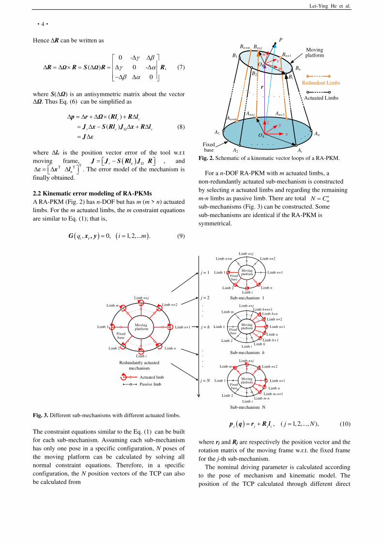
2.2 Kinematic error modeling of RA-PKMs

A RA-PKM (Fig. 2) has n-DOF but has m (m > n) actuated

limbs. For the m actuated limbs, the m constraint equations

are similar to Eq. (1); that is,

( ) ( ), 0, 1,2,... .i

q i m= =iG x , y (9)

. . . . .

A1

A2

An

An+1An+jAn+m

Ai

Bi

B1

B2

Bn

Bn+1

Bn+jBn+m

P

r

. . . .

x

yz

OA

w

v

uOB

Redundant Limbs

Actuated Limbs

Moving platform

Fixed base

Fig. 2. Schematic of a kinematic vector loops of a RA-PKM.

For a n-DOF RA-PKM with m actuated limbs, a

non-redundantly actuated sub-mechanism is constructed

by selecting n actuated limbs and regarding the remaining

m-n limbs as passive limb. There are total n

mN C=

sub-mechanisms (Fig. 3) can be constructed. Some

sub-mechanisms are identical if the RA-PKM is

symmetrical.

Limb n+1Moving

platform

Limb 2

Limb i

Limb n

Limb n+2

Limb n+j

Limb m

Fixed base

Actuated limb

Passive limb

Redundantly actuated mechanism

Movingplatform Limb n+1Limb 1

Limb 2Limb i

Limb n

Limb n+2

Limb n+j

Limb n+m

Fixedbase

MovingplatformFixed

base

Limb n+1Limb 1

Limb 2

Limb i

Limb n

Limb n+2

Limb n+j

Limb m

Limb hLimb h+1

Limb h+n

Limb h+n+1

Movingplatform Limb n+1Limb 1

Limb 2

Limb i

Limb n

Limb n+2

Limb n+j

Limb m

Limb m-nLimb m-n+1

Fixedbase

j = 1

j = 2

j = h

j = N

Sub-mechanism N

Sub-mechanism h

Sub-mechanism 1

Limb 1

Fig. 3. Different sub-mechanisms with different actuated limbs.

The constraint equations similar to the Eq. (1) can be built

for each sub-mechanism. Assuming each sub-mechanism

has only one pose in a specific configuration, N poses of

the moving platform can be calculated by solving all

normal constraint equations. Therefore, in a specific

configuration, the N position vectors of the TCP can also

be calculated from

( ) , ( 1,2,..., ),j j j c

j N= + =p q r R l (10)

where rj and Rj are respectively the position vector and the

rotation matrix of the moving frame w.r.t. the fixed frame

for the j-th sub-mechanism.

The nominal driving parameter is calculated according

to the pose of mechanism and kinematic model. The

position of the TCP calculated through different direct


·5·

kinematic model will be different due to the existence of

kinematic error. In order to solve this problem, the driving

parameters of redundant limbs are adjusted accordingly to

make the mechanism meet the constraint. As a result, it is

assumed that there is no conflict between kinematic limbs

and no deformation of parts in the process of calibration.

Since the sub-mechanism is a part of RA-PKM indeed, the

position of the TCP calculated from different

sub-mechanism is supposed to be consistent.

The N position vectors Pj is supposed to be

1( ) ( ) ( )

j N= =p q p q p q (11)

And the actual position of TCP can be expressed as

1

1

( ) ( ),

. . 1

N

j j

j

N

j

j

s t

=

=

=

=

p q p q

(12)

The error model of the RA-PKM is then written as

1

,N

j j

j

=

= p p (13)

that is, the position error of the RA-PKM can be regarded

as a linear combination of the errors of its

sub-mechanisms. The error model of all its

sub-mechanisms should be developed first to establish the

error model of the RA-PKM. For the j-th sub-mechanism,

as in Eq. (8), the error model can be expressed as

, ( 1,2,..., ),

j j jj N = =p J ε (14)

where Jj and Δεj are the error transfer matrix and kinematic error of the j-th sub-mechanism,

andTT T

j = cε x l .

By substituting Eq. (14) into Eq. (13), the complete error model of the RA-PKM is written

1 1

=N N

j j j j j

j j= =

= = p p J ε J ε (15)

wherein Δε includes kinematic errors Δx of the m limbs

and the geometric error Δlc of the tool, Δlc represent the

position vector error of the tool w.r.t moving frame.

Therefore, before using Eq. (15), all Δεj should be

augmented with Δε, and correspondingly, the Jacobian

matrices Jj also need augment by inserting zero-row

vectors. In this way, the error modeling method applicable

to non-redundant PKM can also be used in the error

modeling of RA-PKM.

3 Example

In this section, the kinematic calibration of a 3-DOF

RA-PKM is studied to verify the proposed method of

error modeling.

3.1 Descriptions of the 3-DOF RA-PKM

RPU Limb UPR Limb

Fixed base

tool

R

P

U

Moving platform

R

P

U

RPU LimbUPR Limb

Fig. 4. Virtual prototype of the 2UPR-2RPU RA-PKM.

A 2UPR-2RPU RA-PKM (Fig. 4) is composed of a fixed

base, a moving platform, a tool, two UPR limbs, and two

RPU limbs. The tool is connected to the center of the

moving platform. Each limb has one universal (U) joint,

one prismatic (P) joint, and one revolute (R) joint, the

prismatic (P) joints with underline denote actuated joints.

The difference in these two types of limbs is the way they

are installed.

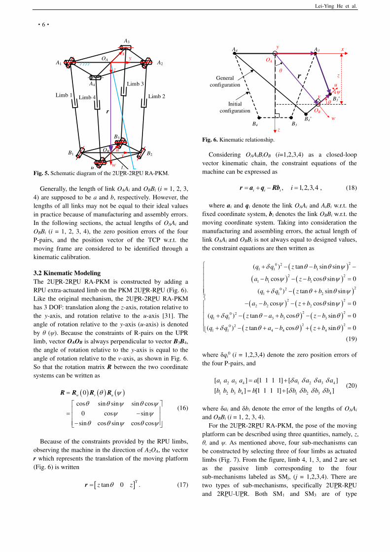
In Fig. 5, the geometrical centers of the universal joints

are the points A1, A2, B3, B4, whereas the intersection

points of the axes of the revolute joints and the axes of the

prismatic joints are the points A3, A4, B1, B2. The TCP of

the mechanism is denoted as P. Points Ai (i = 1, 2, 3, 4)

and Bi (i = 1, 2, 3, 4) form two separate squares, the

centers of which are points OA and OB, respectively. The

fixed frame {OA-xyz} is established at the origin OA with

its z-axis pointing downward and perpendicular to the

fixed base; the x and y axes are parallel to OAA3 and OAA2,

respectively. The moving frame{OB-uvw} is assigned to

point OB with the w-axis vertical to the moving platform;

the u and v axes are parallel to OBB3 and OBB2,

respectively. The axes of the revolute joints and the

universal joints in the fixed base (Fig. 5) are parallel to

either x or y axis, whereas the axes of the joints in the

moving platform are parallel to either u or v axis.

Lei-Ying He et al.

·6·

A1

A3

A2

A4

B1 B2

B3

B4

Limb 1 Limb 2

z

Limb 4

yx

v

w

Limb 3

OA

lc

uOB

r

Fig. 5. Schematic diagram of the 2UPR-2RPU RA-PKM.

Generally, the length of link OAAi and OBBi (i = 1, 2, 3,

4) are supposed to be a and b, respectively. However, the

lengths of all links may not be equal to their ideal values

in practice because of manufacturing and assembly errors.

In the following sections, the actual lengths of OAAi and

OBBi (i = 1, 2, 3, 4), the zero position errors of the four

P-pairs, and the position vector of the TCP w.r.t. the

moving frame are considered to be identified through a

kinematic calibration.

3.2 Kinematic Modeling

The 2UPR-2RPU RA-PKM is constructed by adding a

RPU extra-actuated limb on the PKM 2UPR-RPU (Fig. 6).

Like the original mechanism, the 2UPR-2RPU RA-PKM

has 3 DOF: translation along the z-axis, rotation relative to

the y-axis, and rotation relative to the u-axis [31]. The

angle of rotation relative to the y-axis (u-axis) is denoted

by θ (ψ). Because the constraints of R-pairs on the UPR

limb, vector OAOB is always perpendicular to vector B3B4,

the angle of rotation relative to the y-axis is equal to the

angle of rotation relative to the v-axis, as shown in Fig. 6.

So that the rotation matrix R between the two coordinate

systems can be written as

( ) ( ) ( )0

cos sin sin sin cos

0 cos sin

sin cos sin cos cos

w v u

=

= − −

R R R R

(16)

Because of the constraints provided by the RPU limbs,

observing the machine in the direction of A2OA, the vector

r which represents the translation of the moving platform

(Fig. 6) is written

Ttan 0 .z z=r (17)

x

z

y

OA

A4 A3

B4 B3

B3'

OB

Initialconfiguration

Generalconfiguration

v

w

u

rθ

ψ

B4'

θ

z

Fig. 6. Kinematic relationship.

Considering OAAiBiOB (i=1,2,3,4) as a closed-loop

vector kinematic chain, the constraint equations of the

machine can be expressed as

, 1,2,3,4 ,i i i

i= + − =r a q Rb (18)

where ai and qi denote the link OAAi and AiBi w.r.t. the

fixed coordinate system, bi denotes the link OBBi w.r.t. the

moving coordinate system. Taking into consideration the

manufacturing and assembling errors, the actual length of

link OAAi and OBBi is not always equal to designed values,

the constraint equations are then written as

( )( ) ( )

( )( ) ( )

( ) ( )( ) ( )

20 21 1 1

2 2

1 1 1

20 21 1 2

2 2

2 2 2

2 20 21 1 3 3 3

2 20 21 1 4 4 4

( ) tan sin sin

cos cos sin 0

( ) tan sin sin

cos cos sin 0

( ) tan cos sin 0

( ) tan cos sin 0

q q z b

a b z b

q q z b

a b z b

q q z a b z b

q q z a b z b

+ − − − − − − = + − +

− − − + =

+ − − + − − =

+ − + − + + =

(19)

where δqi0 (i = 1,2,3,4) denote the zero position errors of

the four P-pairs, and

1 2 3 4 1 2 3 4

1 2 3 4 1 2 3 4

[ ] [1 1 1 1] [ ]

[ ] [1 1 1 1] [ ]

a a a a a a a a a

b b b b b b b b b

= +

= + (20)

where δai and δbi denote the error of the lengths of OAAi

and OBBi (i = 1, 2, 3, 4).

For the 2UPR-2RPU RA-PKM, the pose of the moving

platform can be described using three quantities, namely, z,

θ, and ψ. As mentioned above, four sub-mechanisms can

be constructed by selecting three of four limbs as actuated

limbs (Fig. 7). From the figure, limb 4, 1, 3, and 2 are set

as the passive limb corresponding to the four

sub-mechanisms labeled as SMj, (j = 1,2,3,4). There are

two types of sub-mechanisms, specifically 2UPR-RPU

and 2RPU-UPR. Both SM1 and SM3 are of type


·7·

2UPR-RPU PKM, whereas SM2 and SM4 belong to type

of 2RPU-UPR PKM.

The kinematic model of a sub-mechanism can be solved

theoretically. Hereinafter, SM1 is used as an example to

briefly describe the procedure in solving the kinematic

model. For SM1, the first three constraint equations in

Eq. (19) are used. Rewriting and simplifying Eq. (19)

gives

( ) ( )( )

( )

22 1 1 2 1 2 1 2 1 2

22 2 1 1 1 2 2 2 1 1 1 2 1 2

23 3 3

2 cos

( ) 2 sin

sin cos / 2

b k b k b b t b b a a

a b k a b k a b a b t b b a a t

t b t k a

+ = + − + − = − − +

+ = −

(21)

where 0 2 2 2( ) , ( 1,2,3)i i i i i

k q q a b i= + − − = and

/ cost z = . Rearranging the first two equations of

Eq. (21) yields a cubic equation in t2,

( ) ( )2 6 2 4 2 2 2 23 4 1 3 1 2 4 5 22 2 4 0,g t g g g t g g g g t g+ − + − − + = (22)

where 1 2 1 1 2g b k b k= + ,2 2 2 1 1 1 2g a b k a b k= − 3 1 2g b b= + ,

4 2 2 1 1g a b a b= − , 5 1 2 1 2( )g b b a a= + . From the third

equation of Eq. (21), θ is obtained,

2

6 6 3

6 3

2 4 4 ( )2arctan( )

2( )

t t g g b

g b

+ +=

+ (23)

where ( )26 3 32g t k a= − . Since the value z and θ have

been calculated, ψ follows,

23 1 5arccos( ) / 2 .g t g g = − (24)

Hence, the position vector of TCP of SM1 is denoted as

( )1 1 1 ,= + cp q r R l (25)

where r1 and R1 are determined by the obtained values z, θ, and ψ; here lc denotes the actual vector of the TCP w.r.t.

the moving frame. It should be noted that there are

multiple solutions when solving high order equations in

calculation. It is necessary to select the real pose solution

of the mechanism under a specific configuration.

Actuated Limb

Passive Limb

P RU

Moving platform

Sub-Mechanism 1

（2UPR-RPU）

Limb 3

Limb 2 Limb 1

Limb 4

Fixedbase

Sub-Mechanism 2

（2RPU-UPR）

14N C=

Moving platform

Fixedbase

Moving platform

Fixedbase

Moving platform

Fixedbase

Sub-Mechanism 3

（2UPR-RPU）

Sub-Mechanism 4

（2RPU-UPR）

Limb 3

Limb 2 Limb 1

Limb 4

Limb 3

Limb 2 Limb 1

Limb 4

Limb 3

Limb 2 Limb 1

Limb 4

Fig. 7. Four different sub-mechanisms.

Similar to SM1, the kinematic model of the remaining

SMj, (j = 2, 3, 4) can be deduced by the same procedure,

and their corresponding position of TCP, denoted p2, p3,

and p4, can also can be determined.

As introduced in the section 2.2, the actual position of

the TCP can be written

( ) ( )4

1

1.

4j

j=

= p q p q (26)

Here all the coefficients ωj are set to 0.25 to simplify the

calculation according to the constraint condition in Eq.

(12).

3.3 Error modeling

Given the new proposed kinematic model, the error model

Lei-Ying He et al.

·8·

of the 2UPR-2RPU RA-PKM can be presented eventually.

By expanding both sides of Eq. (26) to first-order in

perturbation, the error model of the RA-PKM is written in

the form of

( )4

1

1.

4j

j=

= p p q (27)

As mentioned above, the error models of the four

sub-mechanisms can be obtained firstly by taking a

first-order perturbation expansion on both sides of

Eq. (25); that is,

( ) , 1,2,3,4.j c c

j = + + =p r Ω Rl R l (28)

Considering the first-order terms on both sides of Eq. (16)

and (17), Δr and ΔΩ are written as

T2

T

tan / cos 0

0

z z z

= +

=

r

Ω (29)

Substituting Eq. (29) into Eq. (28), the error model of the

j-th sub-mechanism becomes

2tan / cos 0

0 0 0

1 0 0

0 0 0

( ) 0 1 0

0 0 1

j

c c

z z

z

=

− +

p

S Rl R l

(30)

The first sub-mechanism SM1 is used as an example to

outline briefly how the solution of the error transfer matrix

is obtained. The Eq. (19) can be rewritten as

( ) ( ) ( )( ) ( ) ( )( ) ( )( ) ( )

2 2 221 1 1 1 1 1

2 2 222 2 2 2 2 2

2 223 3 3 3 3

2 224 4 4 4 4

t s s c c s

t s s c c s

t c s

t c s

h q z b a b z b

h q z b a b z b

h q z a b z b

h q z a b z b

= − − − − − − = − + − − − +

= − − + − −

= − + − + + (31)

Considering the first-order linear perturbations on both

side of Eq. (19), we get 0

1 1 1 1 1 1 1 1 1

02 2 1 2 1 2 2 2 2

03 3 1 3 1 3 3 3 3

04 4 1 4 1 4 4 4 4

0

0 ,

0

0

A a B b C q D z E F

A a B b C q D z E F

A a B b C q D z E F

A a B b C q D z E F

+ + + + + =

+ + + + + =

+ + + + + = + + + + + =

(32)

Where

0; ; ;

( 1,2,3,4)

; ; ;

i i i

i i i

i i i

i i i

i i i

h h hA B C

a b qi

h h hD E F

z

= = = = = = =

(33)

The error model of SM1 can be obtained by solving the

first three equations of Eq. (32),

T 01 1 z = J x (34)

where J10 denote the mapping relation between

T z and the kinematic error of SM1.

T0 0 01 1 2 3 1 2 3 1 2 3q q q a a a b b b = x

, and Δqi0 is the zero position errors of the four P-pairs; Δai

and Δbi are the position errors of the U joint and R joint in

the fixed base and moving platform, respectively. Note

that the error parameter Δqi0 stems from the assembly

precision of the prismatic joint rather than the actuated

system. Substituting Eq. (34) into Eq. (30), the error

model of the j-th sub-mechanism is simplified giving

1 1 1, = p J ε (35)

where TT T

1 1 ,c

= ε x l denotes the kinematic error

parameters of SM1, and Δlc denotes the coordinate error of the TCP w.r.t. the moving frame, J1 denote the error mapping matrix.

Similar to SM1, the error model of the remaining SMj (j

= 2, 3, 4) using the same procedure, and their error

transfer matrices J2, J3, and J4 can be obtained. Finally,

from Eq. (27), the complete error model of the RA-PKM

is written as

4 4

1 1

1 1 =

4 4j j j

j j= =

= = p p J ε J ε (36)

4 Kinematic calibration experiments

To validate the error model of the 2RPU-2UPR RA-PKM,

a kinematic calibration experiment was performed (Fig. 8).

A laser tracker (Leica-AT901-LR, Leica Geosystems AG)

was used to measure the 3D coordinate values of the TCP.

The measurement uncertainty for the laser tracker is

±15 μm + 5 μm/m within a 2.5 m × 5 m × 10 m volume.

The repeatability of the prototype of the 2RPU-2UPR

RA-PKM was measured less than 0.15 mm.


·9·

zm

ym

xm

Om

rt

lm

z

yx

vw

OA

lc

P

r

OB u

Fig. 8. Schematic diagram of the error measurement.

4.1 Measurement of errors of the TCP

The nominal and measured positions of the TCP w.r.t.

the fixed frame (Fig. 8) were obtained from

N

M

c

t t m

= +

= +

p r Rl

p r R l (37)

respectively, where Rt and rt are the rotation matrix

and the translation vector of the measurement frame

{Om-xmymzm} w.r.t. the fixed frame, and lm is the

measured position vector of the TCP w.r.t. the

measurement frame. Given the kinematic parameters

and driving parameters, the nominal position of the TCP

pN was calculated by the kinematic model as mentioned

above. The measured value of the TCP pM was obtained

using the laser tracker. The measurement error at one

configuration was defined as the difference between the

nominal and measure values of the TCP. For example,

for the k-th calibration point, its measurement error was

expressed as

( ), , 1,2...k k k c t t m k

k K= + − − =e r R l r R l , (38)

where K is the number of calibration points.

Supposing Rt and rt can be estimated accurately by the

laser tracker, their errors were not taken into account

during the kinematic calibration, and hence

.k k k

= = e p J ε (39)

The whole measurement error of all calibration points

for calibration can be obtained by stacking the

coordinate vectors Eq. (38), that is,

TT T T

1 2 .K

= e e e e (40)

Substituting Eq. (39) into Eq. (40) yields

TT T T

1 2 ,K

= = e e e e M ε (41)

where TT T T

1 2 K = M J J J is the identification

matrix, and Jk (k = 1, 2…K) is the Jacobian matrix of

measurement error of the TCP relative to the kinematic

error given in Eq. (36).

4.2 Parameters identification

During error identification, the object function and the

fitting method need to be established. The error

identification of the PKM can normally be converted to

a minimization problem,

arg min =ε e . (42)

The minimization is a nonlinear least square problem

with an iterative relation. To solve this problem, various

methods have been proposed, such as the

Levenburg–Marquardt algorithm [32], the Kalman

filtering approach [33], and the Ridge estimation method

[34, 35]. Here it given as

( ) 1T T1 ,

t t

−

+ = + ε ε M M M e (43)

where t represents the iteration times, M denote the

identification matrix which is defined in Eq. (41). The

termination condition of the iteration is that the error

residual ||Δe|| or the change in Δε between two adjacent

iterations is sufficiently small.

For the selection of the measurement configurations,

the calibration is well performed in a sensitive area of

the entire workspace, for example, the boundary of the

workspace. The workspace of the 2UPR-2RPU machine

with a tool of [0 0 125]T is shown in Fig. 9. Three

ellipses on the surface that fit the shape of the boundary

of the workspace were constructed with the intention to

take a certain number of calibration points distributed

evenly on these ellipses.

To avoid parameter identification failure caused by

the singularity of the identification matrix, the number

of calibration points also has certain requirements. Since

there are in total 15 kinematic errors considered in the

error model, here 16 calibration points on each ellipse,

totally 48 calibration points in the workspace (Fig. 9),

were selected. That is, the number of calibration points

is more than twice the number of error parameters to be

identified, thus ensuring the validity and accuracy of the

calibration[36].

Lei-Ying He et al.

·10·

Workspace

Calibration point

Fig. 9. Distribution of the calibration points within the workspace.

4.3 Experiments

A calibration experiment on the parallel manipulator

using a laser tracker was performed (Fig 10). The

rotation matrix Rt and translation vector rt of the

measurement frame {Om-xmymzm} w.r.t. the fixed frame

was measured to be

T

0.0008 0.9999 0.0025

0.9999 0.0008 0.0045

0.0045 0.0025 0.9999

50.402 2348.299 35.523

t

t

− = −

= − −

R

r

which is obtained through the fitting of plane, and the

unit of rt is millimeter. Table 1 lists the values of the

nominal kinematic parameters for this mechanism. The

initial kinematic errors are set to zero.

2UPR-2RPU

RA-PKM

Laser tracker

Measurement

system

control

system

Reflector

Fig 10 Kinematic calibration experiment.

Table 1 Kinematic parameters of the mechanism

Parameters a b Range of qi (i =1,2,3,4)

lc

values/mm 150 60 [245,345] [0 0 125]T

The calibration comprises four steps: error modeling,

error measurement, parameter identification, and error

compensation, and its procedure is shown in Fig. 11.

Fig. 11. Procedure of the kinematic calibration.

Jia-Fan Zhang et al.

11

·11·

4.4 Results and discussion

Since the machine has three DOFs: two rotational DOFs

and one translational DOF, three independent motion

parameters ψ, θ and z are sufficient to describe the configuration of the moving platform. However, it is

impossible to compare these three parameters in a space

uniformly, because their dimensions are not the same.

Alternatively, the position vector of the TCP p = [px py

pz]T is something should be paid more attention to when

calibrating, whose error denotes the position error and

orientation error of moving platform. In this paper, the

position vector p, which can be expressed by three

motion parameters ψ, θ and z using Eq. (4), replaces

these three parameters to analyze the accuracy of the

machine. The position error and orientation error of

moving platform can be denoted by the position error of

TCP.

Fig. 12 shows the errors of 48 calibration points

(position errors of TCP) before and after calibration. The

mean, maximum, and standard derivation of the position

residual decrease from 3.427 mm to 0.177 mm, from

4.740 mm to 0.384 mm, and from 0.547 mm to

0.084 mm, respectively. In other words, the calibration

significantly reduces the residuals.

Calibration point No.

Erro

r e

k (

mm

)

Mean = 3.427Max = 4.740Std. = 0.547Mean = 0.177

Max = 0.384Std. = 0.084

Fig. 12. Position errors before and after calibration.

The kinematic error parameters of the 2UPR-2RPU

RAPAM are identified as

T

T

T0

T

0.406 0.985 1.376 1.554

0.062 0.190 3.266 2.480

0.086 2.116 2.365 1.695

0.095 0.204 0.087

= − −

= −

= −

= −c

a

b

q

l

For an actual mechanism, Δa and Δb are the

deviations of distances from the U-pair and R-pair to the

center of the fixed base and moving platform,

respectively, Δq0 is the error of the origin position of the

P-pair, and Δlc the position deviation of the TCP w.r.t.

the moving platform. The calibration result shows that

Δa1 and Δa2 were smaller than Δa3 and Δa4 because the

accuracy of the length of link A1A2 is easier to ensure

than that of A3A4 in the assembly process. Also, Δb3 and

Δb4 were larger than Δb1 and Δb2 because the former

represent the position error of the U joint and the latter

are those of the R joint. Recall that, in terms of

manufacturing and assembly, the U-pair is more

complex than the R-pair.

To verify the effect of compensation with the

identified kinematic parameters in the whole workspace,

some test points, either inside or outside the calibration

area, are chosen. The distribution of test points (Fig. 13)

show that their distribution characteristics are basically

the same as those of the calibration points. The

difference is the distance from the point to the boundary

of the workspace. Of course, these test points are still in

the workspace. The driving parameter is calculated with

the compensated kinematic model; the result is

presented in Fig. 14.

Calibration point

Test point (inside)

Test point(outside)

x/mmy/mm

z/m

m

Fig. 13. Distribution of test points

Calibration point No.

Err

or e

k (

mm

)


Fig. 14. Compensation results in different areas.

Table 2 Statistics of the positioning error after compensation

Statistical values

No. Mean /mm

Std. /mm

Maximum /mm

Calibration points

48 0.177 0.084 0.384

Inside testing points

48 0.366 0.126 0.764

Outside testing points

48 0.439 0.190 0.845

In the test area outside the calibration area, the mean

and maximum values of the deviation in position

decreased from 3.570 mm and 4.767 mm to 0.440 mm

and 0.845 mm, respectively. With the test area inside the

calibration area, the mean and maximum values of the

deviation in position decreased from 2.832 mm and

3.606 mm to 0.366 mm and 0.764 mm, respectively. The

conclusion drawn from Fig. 14 is that, regardless of the

location of the test point, the deviation in position is

significantly reduced after compensation, thereby

demonstrating the effectiveness of this calibration in the

whole workspace and showing that in practice the

proposed error model is suitable for the 2UPR-2RPU

RA-PKM. Nevertheless, the compensated result from

the test area is seen to be not as ideal as in the

calibration area. Also, the compensation results of the

test points inside the calibration area are slightly better

than those outside the calibration area. The reason is that

the closer the test point is to the boundary of the

workspace, the more significant the effect of sources of

error on the deviation in position.

Although, the error of the RA-PKM will decrease

dramatically after kinematic calibration using the

proposed error modeling, some challenges and

limitations still exist. The accuracy of the error model is

dependent heavily on the distribution of weight

coefficients ω in Eq. (13). Actually, the weight

coefficients ω are affected both by the stiffness and

geometric errors of the links. However, their clear

relationship is difficult to establish. For simplification,

equal weight coefficients were determined in the paper,

which is an approximate and simple solution, but still

effective for kinematic calibration. To further improve

the accuracy of the error model, a more approximate

influence of weight coefficients should be studied in the

future work.

5 Conclusions

A new error modeling method for kinematic calibration

of RA-PKMs is presented considering the kinematic

errors. The complete geometric error model of a

RA-PKM can be calculated as the weighted summation

of error models of all non-redundantly actuated

sub-mechanisms which keep the same mobility as the

PA-PKM. The proposed method is verified to be

effective through a kinematic calibration experiment

using a 3-DOF 2UPR-2RPU RA-PKM. It is shown that

the mean positioning error of the TCP of the RA-PKM is

decreased from 3.427 mm to 0.177 mm after kinematic

calibration, which shows the improvement of the

accuracy of the RA-PKM. Additionally, the result of the

experiment also indicates the effectiveness of the

parameters compensation after kinematic calibration in

the whole workspace.

6 Declaration

Acknowledgements

Not applicable.

Funding

Supported by National Natural Science Foundation of

China (Grant Nos. 51525504, and U1713202), and Natural

Science Foundation of Zhejiang Province ((Grant No.

LQ19E050015).

Availability of data and materials

The datasets supporting the conclusions of this article

are included within the article.

Authors’ contributions

The author’ contributions are as follows: QL was in

charge of the whole trial; ZW and LH wrote the

manuscript; XC assisted with sampling and laboratory

analyses.

Competing interests

The authors declare no competing financial interests.

Consent for publication

Not applicable

Ethics approval and consent to participate

Not applicable

A new method for error modeling in the kinematic calibration of redundantly actuated parallel kinematic machine ·13·

References

[1] Kim, J., Park, F. C., Ryu, S. J., Kim, J. (2012). Design and analysis

of a redundantly actuated parallel mechanism for rapid machining.

IEEE Transactions on Robotics & Automation, 17(4), 423-434.

[2] Luces, M., Mills, J. K., & Benhabib, B. (2017). A review of

redundant parallel kinematic mechanisms. Journal of Intelligent &

Robotic Systems, 86(2), 175-198.

[3] Sadjadian, H., & Taghirad, H. D. (2006). Kinematic, singularity and

stiffness analysis of the hydraulic shoulder: a 3-d.o.f. redundant

parallel manipulator. Advanced Robotics the International Journal

of the Robotics Society of Japan, 20(7), 763-781.

[4] Mueller, A. (2013). On the terminology and geometric aspects of

redundant parallel manipulators. Robotica, 31(1), 137-147.

Andreas, M., 2013, "On the terminology and geometric aspects of

redundant parallel manipulators" Robotica, 31(1), pp. 137-147.

[5] Cheng, G., Yu, J. L., & Gu, W. (2012). Kinematic analysis of

3sps+1ps bionic parallel test platform for hip joint simulator based

on unit quaternion. Robotics and Computer Integrated

Manufacturing, 28(2), 257-264.

[6] Bennett, D. J., & Hollerbach, J. M. (1991). Autonomous calibration

of single-loop closed kinematic chains formed by manipulators

with passive endpoint constraints. IEEE Transactions on Robotics

& Automation, 7(5), 597-606.

[7] Lee, M. K., Kim, T. S., Park, K. W., & Kwon, S. H. (2003).

Constraint operator for the kinematic calibration of a parallel

mechanism. Journal of Mechanical Science and Technology, 17(1),

23-31.

[8] Ren, X. D., Feng, Z. R., & Su, C. P. (2009). A new calibration

method for parallel kinematics machine tools using orientation

constraint. International Journal of Machine Tools & Manufacture,

49(9), 708-721.

[9] Zhuang, H. (1997). Self-calibration of parallel mechanisms with a

case study on Stewart platforms. IEEE Transactions on Robotics &

Automation, 13(3), 387-397.

[10] Andreff, N., & Martinet, P. (2009). Vision-based self-calibration

and control of parallel kinematic mechanisms without

proprioceptive sensing. Intelligent Service Robotics, 2(2), 71-80.

[11] Wu, J. F., Zhang, R., Wang, R. H., & Yao, Y. X. (2014). A

systematic optimization approach for the calibration of parallel

kinematics machine tools by a laser tracker. International Journal

of Machine Tools and Manufacture, 86(6), 1-11.

[12] Jeong, J. I., Kang, D., Cho, Y. M., & Kim, J. (2004). Kinematic

calibration for redundantly actuated parallel mechanisms. Journal

of Mechanical Design, 126(2), 1211-1217.

[13] Nubiola, A., & Bonev, I. A. (2014). Absolute robot calibration with

a single telescoping ballbar. Precision Engineering, 38(3), 472-480.

[14] Traslosheros, A., Sebastián, J. M., Torrijos, J., Carelli, R. &

Castillo, E. (2013). An Inexpensive Method for Kinematic

Calibration of a Parallel Robot by Using One Hand-Held Camera as

Main Sensor. Sensors, 13(8), 9941-9965.

[15] Du, G., & Zhang, P. (2013). Online robot calibration based on

vision measurement. Robotics & Computer Integrated


[16] Motta, J. M. C. S. T., Carvalho, G. C. D. & Mcmaster, R. S. (2001).

Robot calibration using a 3D vision-based measurement system

with a single camera. Robotics and Computer-Integrated


[17] G., W. A. D. (1992). Fundamentals of manipulator calibration.

Microelectron. Reliab, 32(s1–2), 275–276.

[18] Klimchik, A., Caro, S. & Pashkevich, A. (2015). Optimal pose

selection for calibration of planar anthropomorphic manipulators.

Precis. Eng.-J. Int. Soc. Precis. Eng. Nanotechnol., 40(9), 214-229.

[19] Zhuang, H., Wang, L. K. & Roth, Z. S. (1993). Error-model-based

robot calibration using a modified CPC model. Robot. Comput.

-Integr. Manuf.,10(4), 287-299.

[20] Park, & F., C. (1994). Computational aspects of the

product-of-exponentials formula for robot kinematics. IEEE

Transactions on Automatic Control, 39(3), 643-647.

[21] Liu, H., Huang, T., & Chetwynd, D. G. (2011). A general approach

for geometric error modeling of lower mobility parallel

manipulators. Journal of Mechanisms & Robotics, 3(2), 021013.

[22] Huang, T., Liu, H. T. and Chetwynd, D. G. (2011). Generalized

Jacobian analysis of lower mobility manipulators. Mech. Mach.

Theory, 46(6), 831-844.

[23] Hollerbach, J. M., & Lokhorst, D. M. (1993). Closed-loop

kinematic calibration of the RSI 6-dof hand controller. IEEE

Transactions on Robotics & Automation, 11(3), 352-359.

[24] Wampler, C. W., Hollerbach, J. M. & Arai, T. (1995). An implicit

loop method for kinematic calibration and its application to

closed-chain mechanisms. IEEE Transactions on Robotics and

Automation, 11(5), 710-724.

[25] Ecorchard, G., Neugebauer, R., & Maurine, P. (2010).

Elasto-geometrical modeling and calibration of redundantly

actuated PKMs. Mechanism & Machine Theory, 45(5), 795-810.

[26] Jeon, D., Kim, K., Jeong, J. I., & Kim, J. (2010). A calibration

method of redundantly actuated parallel mechanism machines

based on projection technique. CIRP Annals - Manufacturing

Technology, 59(1), 413-416.

[27] Muller A., & Ruggiu, M. (2012). Self-calibration of redundantly

actuated PKM based on motion reversal points. In: Lenarcic J.,

Husty M. (eds), Latest Advances in Robot Kinematics (pp.75-82).

Dordrecht: Springer.

[28] Ruggiu, M., & Muller A. (2019). Self-calibration of RA-PKM via

motion reverse points: A procedure based on an analytical indicator

function. Mechanics Based Design of Structures and Machines,

47(5), 621-628.

[29] Lee G., Jeong J. I. & Kim J. 2016. Calibration of encoder indexing

of a redundantly actuated parallel mechanism to eliminate

contradicting control forces. Mechanics Based Design of Structures

and Machines, 44(4), 306 - 316.

[30] Chen, I. M., Yang, G., Tan, C. T., Song, H., & Yeo. (2001). Local

POE model for robot kinematic calibration. Mechanism and

Machine Theory, 36(11), 1215-1239.

[31] Wang, F., Chen, Q., & Li, Q. (2015). Optimal design of a 2-upr-rpu

parallel manipulator. Journal of Mechanical Design, 137(5),

054501.

[32] Majarena, C, A., Santolaria, Samper, Aguilar & J, J. (2013).

Analysis and evaluation of objective functions in kinematic

calibration of parallel mechanisms. International Journal of

Advanced Manufacturing Technology, 66(5-8), 751-761.

[33] Nguyen, H. N., Zhou, J., & Kang, H. J. (2015). A calibration

method for enhancing robot accuracy through integration of an

extended Kalman filter algorithm and an artificial neural network.

Neurocomputing, 151, 996-1005.

[34] Sun, T., Wang, P., Lian, B., Liu, S., & Zhai, Y. (2017). Geometric

accuracy design and error compensation of a one-translational and

three-rotational parallel mechanism with articulated traveling plate.

Proceedings of the Institution of Mechanical Engineers Part B


Journal of Engineering Manufacture, 095440541668343.

[35] Sun, T., Zhai, Y., Song, Y., & Zhang, J. (2016). Kinematic

calibration of a 3-dof rotational parallel manipulator using laser

tracker. Robotics and Computer Integrated Manufacturing, 41,

78-91.

[36] A. Nubiola., & I.A. Bonev. (2014). Absolute calibration of an ABB

IRB 1600 robot using a laser tracker. Robotics & Computer

Integrated Manufacturing, 29(6), 236-245.

Biographical notes

Lei-Ying He, born in 1983, is currently a Lecturer at Faculty of Mechanical Engineering & Automation, Zhejiang Sci-Tech University, China. He received his PhD. degree from Zhejiang Sci-Tech University, China, in 2014. His research interests include kinematic calibration and robot vision. E-mail: [email protected] Zhen-Dong Wang, born in 1993, received his master degree in Zhejiang Sci-Tech University, China, in 2019. His research interest is the error modelling and kinematic calibration of parallel mechanisms. E-mail: [email protected] Qin-Chuan Li, born in 1975, is currently an professor at Faculty

of Mechanical Engineering & Automation, Zhejiang Sci-Tech

University, China. He received his PhD degree from Yanshan

Universtiy, China, in 2003. His research interests include mechanism and machine theory. E-mail: [email protected] Xin-Xue Chai, born in 1988, is currently a lecture at Faculty of Mechanical Engineering & Automation, Zhejiang Sci-Tech University, China. She received her PhD. degree from Zhejiang Sci-Tech University, China, in 2017. Her research interests is mechanism theory using geometric algebra. E-mail: [email protected]

Figures

Figure 1

Figure 1

Figure 2

Figure 2

Figure 3

Figure 3

Figure 4

Figure 4

Figure 5

Figure 5

Figure 6

Figure 6

Figure 7

Figure 7

Figure 8

Figure 8

Figure 9

Figure 9

Figure 10

Figure 10

Figure 11

Figure 11

Figure 12

Figure 12

Figure 13

Figure 13

Figure 14

Figure 14

a new method for error modeling in the kinematic

Documents