kinematic and dynamic modeling of nanostructured origami
TRANSCRIPT

Kinematic and Dynamic Modeling of Nanostructured Origami
by
Paul Steven Stellman
B.S., Texas A&M University (2004)
Submitted to the Department of Mechanical Engineeringin partial fulfillment of the requirements for the degree of
Master of Science
at the
MASSACHUSETTS INSTITUTE OF TECHNOLOGY
February 2006
@ Paul Steven Stellman, 2006. All rights reserved.
The author hereby grants to Massachusetts Institute of Technology permission toreproduce and
to distribute copies of this thesis document in whole or in part.
Signature of A uthor.............. ...................................................Department of Mechanical Engineering
25 January 2006
Certified by ........
Accepted by................
C
MASSACHUSETTS INSTITUTEOF TECHNOLOGY
JUL 14 2006
LIBRARIESBARKER
........................ ...George Barbastathis
Associate Professor of Mechanical EngineeringA Research Head
................Lallit Anand
hairperson, Department Committee on Graduate Students

Kinematic and Dynamic Modeling of Nanostructured Origami
by
Paul Steven Stellman
Submitted to the Department of Mechanical Engineeringon 25 January 2006, in partial fulfillment of the
requirements for the degree ofMaster of Science
Abstract
Nanostructured Origami is a manufacturing process that folds nanopatterned thin films intoa desired 3D shape. This process extends the properties of 3D design and connectivity foundin origami artwork to the bulk fabrication of 3D nanostructures. Our technique is a two-stepprocedure that first patterns the devices in 2D and then folds the membranes to the final 3Dshape along pre-defined creases.
This thesis describes theoretical methods that have been developed to model the actuation oforigami devices. The background of origami mathematics and advances in robotics are presentedin the context of modeling Nanostructured Origami. Unfolding of single-vertex origami isdiscussed, and an algorithm is implemented to calculate the unfolding trajectories of severaldevices. Another contribution of this thesis is the presentation of a methodology for modelingthe dynamics of two classes of origami: accordion origamis and single-vertex origamis. Theforward dynamics and equilibrium analysis of a useful bridge structure and the corner cubeorigami are simulated. The response of a model of an experimental actuation technique is well-behaved, and it is shown that the final folded state of these devices is at a stable equilibrium.
Research Head: Prof. George BarbastathisTitle: Associate Professor of Mechanical Engineering
2

0.1 Foreword
My short tenure as a graduate student has been an amazing time in my life! I have learned
many valuable lessons and forged new relationships that I will carry with me for the rest of
my life. MIT has offered me an educational experience that has given me a new perspective
on life-long learning. The research presented in this thesis has been an exciting pursuit, and I
look forward to continuing my work toward a PhD.
There were many people who made significant contributions to this thesis. First and fore-
most among these people is my advisor, Professor George Barbastathis. His unyielding support
for my work was comforting, and his unmatched enthusiasm radiates toward everyone in his
presence. The most rewarding moments, however, were those many one-on-one meetings in
which we discussed my research at length. Whether I was tired and out of new ideas or work-
ing in the wrong direction entirely, the meetings with George always seemed to spark new
enthusiasm toward my research.
Special thanks goes to Professor Erik Demaine of MIT as well. His research in origami math-
ematics is making rapid advances. I appreciate his conversations with George and me regarding
the unfolding of single-vertex origamis, and I am privileged to have been his collaborator.
All my colleagues in the 3D Optical Systems Group were essential to my academic success.
There are five students in the group working on the Nanostructured Origami project, and I am
excited about the progress that we will make in the future. Special thanks to Tilman Buchner,
Will Arora, Hyun Jin In, Tony Nichol, and Nader Shaar for the numerous research discussions
and for all of your support for our project. I would also like to thank Satoshi Takahashi for
helping me with the research of Chapter 3 during a class in 2004.
I would like to thank my mother, Kay Tettleton, for her unwavering support of me and my
career. I truly could not have done it without her help. Also, my stepfather, John Tettleton, has
always been supportive of my endeavors and has encouraged me to pursue a career and lifestyle
with which I will be happy. Thanks also to my father, Steve Stellman, for his confidence
in my abilities and his encouragement. Finally, I would like to thank my girlfriend, Laurie
Friesenhahn, for the companionship and love we have shared over the past 15 months.
Cambridge, MA
January 2006
3
Contents
0.1 Forew ord . . . . . . . . . . . . . . . . . . . . . . . . . . . . . . . . . . . . . . .
1 Introduction
1.1 Inspiration . . . . . . . . . . . . .
1.2 Applications. . . . . . . . . . . . .
1.3 Actuation Methods . . . . . . . . .
1.4 Overview of the Thesis. . . . . . .
2 Background
2.1 Geometry of Folding and Unfolding
2.1.1 Unfolding Techniques . . .
2.1.2 Origami . . . . . . . . . . .
2.2 Robot Dynamics and Control . . .
3 Unfolding Single-Vertex Origamis
3.1 Energy Methods for Unfolding . .
3.2 Simulation Results . . . . . . . . .
4 Folding Dynamics
4.1 Origami Topology . . . . . . . . .
4.2 Kinematics . . . . . . . . . . . . .
4.3 Constraints . . . . . . . . . . . . .
4.4 Open Chain Equations of Motion
4.5 Closed Chain Equations of Motion
8
9
12
. . . . . . . . . . . . . . 14
. . . . . . . . . . . . . . 1 5
16
16
16
17
19
21
22
25
28
29
30
32
33
35
4
.3
. . . . . . . . . . . . . . . . . . . . . . . . . .
. . . . . . . . . . . . . . . . . . . . . . . . . .
. . . . . . . . . . . . . . . . . . . . .
. . . . . . . . . . . . . . . . . . . . .
. . . . . . . . . . . . . . . . . . . . .
. . . . . . . . . . . . . . . . . . . . .
. . . . . . . . . . . . . . . . . . . . .
. . . . . . . . . . . . . . . . . . . . .
. . . . . . . . . . . . . . . . . . . . .

5 Examples
5.1 Accordion Origami .....
5.1.1 Geometry . . . . . .
5.1.2 Equations of Motion
5.1.3 Forward Dynamics .
5.1.4 Stability . . . . . . .
5.2 Corner Cube Origami . . .
5.2.1 Geometry . . . . . .
5.2.2
5.2.3
5.2.4
5.2.5
37
37
37
. . . . . . . . . . . 40
Equations of Motion
Forward Dynamics .
Ramp Input . . . . .
Stability . . . . . . .
6 Conclusions and Future Work
6.1 Single-Vertex Unfolding . . . . .
6.2 Simulation of Origami Dynamics
6.3 Future Work . . . . . . . . . . .
I Appendix A: Geometric and Material Parameters for Bridge
II Appendix B: Geometric and Material Parameters for Corner Cube
42
45
47
47
51
52
53
55
57
57
57
58
60
79
5
. . . . . . . . . . . . . . . . . . . . .
. . . . . . . . . . . . . . . . . . . . .
. . . . . . . . . . .
. . . . . . . . . . .

List of Figures
1-1 Cartoon of folded origamis on a wafer. . . . . . . . . . . . . . . . . . . . . . . . . 9
1-2 Various origami artwork made by Robert Lang. Copyright Robert Lang. . . . . . 10
1-3 3D surface map of cerebral cortex. Copyright SumsDB 2006. . . . . . . . . . . . 10
1-4 3D model of the protein hemoglobin. Copyright Pittsburgh Supercomputing
C enter 2006 . . . . . . . . . . . . . . . . . . . . . . . . . . . . . . . . . . . . . . . 11
1-5 Schematic of supercapacitor (a) before folding and (b) after folding. SEM plots
of actual device (c) before folding and (d) after folding. Copyright Hyun Jin In
2005.......... ............................................ 13
1-6 Schematic of 3D photonic crystal fabricated using origami . . . . . . . . . . . . . 13
1-7 Diagram of chiral material proposed as a negative refractive material. Copyright
J. Pendry 2004. . . . . . . . . . . . . . . . . . . . . . . . . . . . . . . . . . . . . . 14
1-8 Drawing of the Lorentz force actuation procedure. . . . . . . . . . . . . . . . . . 15
2-1 The unlocking of 2D linkages using pseudotriangulations. Copyright Ileana
Streinu 2004. . . . . . . . . . . . . . . . . . . . . . . . . . . . . . . . . . . . . . . 18
2-2 Unfolding of 2D chain using energy method. Copyright Cantarella, et al 2004. . . 18
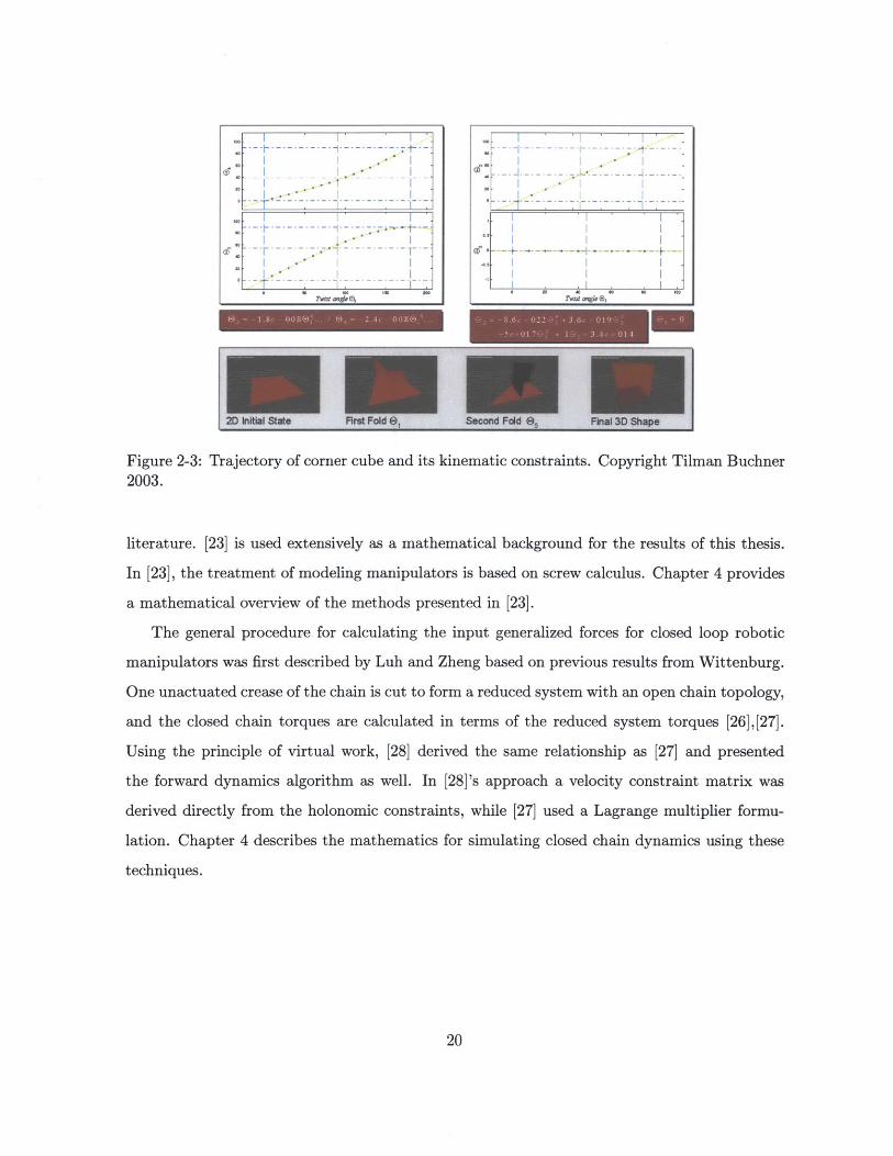
2-3 Trajectory of corner cube and its kinematic constraints. Copyright Tilman Buch-
ner 2003. ......... ........................................ 20
3-1 (a) Corner cube crease pattern and folded state and (b) Origami fold that is
disallowed due to self-intersections . . . . . . . . . . . . . . . . . . . . . . . . . . 22
3-2 Crease pattern and folded corner cube. . . . . . . . . . . . . . . . . . . . . . . . . 23
3-3 Half-paper unfolding . . . . . . . . . . . . . . . . . . . . . . . . . . . . . . . . . . 26
6

3-4 Unfolding of corner cube origami . . . . . . . . . . . . . . . . . . . . . . . . . . . 26
3-5 Water-bomb base unfolding path . . . . . . . . . . . . . . . . . . . . . . . . . . . 26
4-1 Schematic of n-link accordion origami. . . . . . . . . . . . . . . . . . . . . . . . . 29
4-2 Schematic of arbitrary single-vertex origami . . . . . . . . . . . . . . . . . . . . . 30
5-1 Accordion origamis actuated using a stressed bilayer. . . . . . . . . . . . . . . . . 38
5-2 (a) Crease pattern of bridge device and (b) the bridge in its folded state. . . . . . 39
5-3 Diagram of thin film bilayer used in stress actuation technique. . . . . . . . . . . 41
5-4 Step response of bridge device until collision. . . . . . . . . . . . . . . . . . . . . 43
5-5 Schematic of KOH etch of single segment. . . . . . . . . . . . . . . . . . . . . . . 44
5-6 Ramp response plots for bridge device. . . . . . . . . . . . . . . . . . . . . . . . . 46
5-7 Trajectory of bridge resulting from ramp input. . . . . . . . . . . . . . . . . . . . 46
5-8 Schematic of (a) original closed chain corner cube and (b) reduced open chain
system . . . . . . . . . . . . . . . . . . . . . . . . . . . . . . . . . . . . . . . . . . 48
5-9 Holonomic constraint relation for corner cube . . . . . . . . . . . . . . . . . . . . 50
5-10 Step response of corner cube until collision. . . . . . . . . . . . . . . . . . . . . . 53
5-11 Ramp response of corner cube . . . . . . . . . . . . . . . . . . . . . . . . . . . . . 54
5-12 Trajectory of corner cube resulting from a ramp input. . . . . . . . . . . . . . . . 55
7

Chapter 1
Introduction
This thesis describes analytical and numerical modeling techniques used to design and char-
acterize the folding of nanopatterned membranes. The process of patterning devices in 2D
and folding to a desired 3D shape is referred to as Nanostructured Origami [1]. Fig. 1-1
shows a schematic of several folded devices on a silicon wafer. The surfaces of the segments
can be patterned with any number of devices, including optical, electronic, microfluidic, and
mechanical structures. The 2D patterning step is accomplished using any of the industrial or
research-grade writing methods such as optical lithography, electron beam lithography, and
nanoimprinting. The extensive infrastructure of the semiconductor industry allows this step
to be included seamlessly with the origami process, while maintaining the highest patterning
resolutions available for the devices [2]. To facilitate the folding of the origami membranes,
active and passive creases are also patterned during the first step. Active creases are designed
to contain the functionality necessary to actuate the folding motion, while passive creases are
thinned films that fold in response to actuation at the active creases.
The second step of Nanostructured Origami is to accurately and repeatedly fold the segments
to the desired positions. This requires the actuation method to be controllable and compatible
with the fabrication technology. Once a model has been developed for the actuation at a
crease, it is possible to predict the motion of the origami system mathematically. The actuation
procedure can be modeled as an external torque applied to the creases of the origami, and the
required torques can be calculated directly from the origami's geometry and material properties.
By gaining knowledge of origami geometry and the system dynamics, the actuation sequence
8

Figure 1-1: Cartoon of folded origamis on a wafer.
can be implemented such that the origami folds correctly to the desired folded state. The
concepts introduced in this thesis can also be extended to the case of more complex origamis.
1.1 Inspiration
The inspiration for 3D nanomanufacturing comes from the observation that there is an in-
herent advantage to using all three geometric dimensions. However, the fabrication of three-
dimensional nanostructures is difficult. Current methods are limited largely to either periodic
structures fabricated using interferometric lithography or stacked devices formed by multiple
sacrificial etches [3]. For non-periodic structures, no other efficient manufacturing method has
been developed. The idea for folding patterned thin films arises from both the Japanese art
of origami and folding that is observed in nature. Master origamists such as Robert Lang can
fold magnificent shapes such as those in Fig. 1-2. Although these shapes are pieces of art with
no practical use in nanomanufacturing, the figure illustrates both the high level of connectivity
and 3D effectiveness that origami offers. The patterning step in our process gives definition to
these surfaces that provides the 3D functionality of Nanostructured Origami.
Consider the schematic of the human brain's cerebral cortex in Fig. 1-3. Washington Uni-
9

Figure 1-2: Various origami artwork made by Robert Lang. Copyright Robert Lang.
Figure 1-3: 3D surface map of cerebral cortex. Copyright SumsDB 2006.
10

Figure 1-4: 3D model of the protein hemoglobin. Copyright Pittsburgh Supercomputing Center
2006.
versity neuroscientists created this 3D atlas of the folds of the cerebral cortex. Their study
maps the folds in the cerebral cortex to brain function. The surface map, called PALS, is a
clear example of the 3D functionality that nature has imparted to the brain through folding.
These 3D neural connections have high volumetric efficiency and are prime examples of the
advantages of 3D interconnections [4].
Another example of the advantages of folding is in the self-assembly of proteins. Proteins
are the building blocks of all biological organisms. They consist of a sequence of amino acids
that fold themselves into a specific shape. The ultimate goal of the Human Genome Project
was to determine the sequence of amino acids for any human protein. This sequence, absent
any folding, is simply a one-dimensional string of information that is produced inside the ribo-
some. The major reason for the protein's functionality, however, is its ability to repeatably and
accurately fold to an expected shape. Consider the image in Fig. 1-4 of the protein hemoglobin,
which carries oxygen through the bloodstream [51. This remarkable function is accomplished
because its geometry (and the physics associated with its geometry) has been assembled very
accurately by forces applied to the chain as it leaves the ribosome.
11

Analogously, the patterning step in Nanostructured Origami is essentially a two-dimensional
surface of information that is written onto a silicon wafer. Electronic, optical, and other types of
information are encoded on the wafer surface at very high information density. Similarly, Nanos-
tructured Origami folds a pre-patterned surface into the desired shape. The self-assembly of the
origami's folding on a wafer is critical in making complex shapes. Unlike larger 3D man-made
structures, such as skyscrapers, the small length scales that define both proteins and nanopat-
terned origamis necessitate automatic folding processes. Systems such as the Atomic Force
Microscope (AFM) can manipulate matter on the atomic scale, but the AFM writes serially
and hence is inefficient for bulk fabrication. Just as computational modeling has been essential
in understanding the structure of proteins [6],[18], modeling facilitates a deeper understanding
of the self-actuation of origami.
1.2 Applications
The previous section described our motivation for pursuing the development of a robust 3D
nanomanufacturing technique. Given that Nanostructured Origami is a generic manufacturing
process, there is not one specific application that we are trying to employ. Instead, the origami
process should be viewed as a platform for making arbitrary shapes. A few example applications
include an electrochemical supercapacitor, 3D photonic crystals, negative index materials, a
corner cube retroreflector, and a bridge device for optical interconnects. The supercapacitor,
photonic crystals, and negative index material will briefly be described in this section, while
the corner cube and bridge are analyzed and modeled in Chapter 5.
An electrochemical supercapacitor was created using the Nanostructured Origami technique
and is presented in [7]. The device is a type of accordion origami in which an electrode coated
in some form of carbon is folded over a fixed electrode. The device can be used as a power
source for any number of microelectromechanical systems. Testing indicates that the increased
surface area due to folding creates a high capacitance. A schematic of the supercapacitor and
scanning electron micrographs of the actual SU-8 device are shown in Fig. 1-5.
Photonic crystals are a class of integrated optical devices that hold great promise in the
12

SU-8 flap
(a) (b)
Figure 1-5: Schematic of supercapacitor (a) before folding and (b) after folding. SEM plots ofactual device (c) before folding and (d) after folding. Copyright Hyun Jin In 2005.
Figure 1-6: Schematic of 3D photonic crystal fabricated using origami.
area of optical computing and communications. Currently, 3D photonic crystals are made by
stacking [3]. These devices act as waveguides, and they could potentially be manufactured by
folding as an accordion origami. Fig. 1-6 illustrates the accordion concept as applied to a 3D
photonic crystal. The major concern when making a photonic crystal is ensuring nanometer-
scale alignment. This could potentially be done using nanomagnets or another form of precision
alignment technique.
A third application is the fabrication of materials that exhibit a negative index of refrac-
tion. Among other applications, these materials can act as "perfect lenses" by amplifying the
evanescent optical field. This could potentially beat the diffraction limit for imaging and in the
lithography industry. [8] has described a chiral material that exhibits a negative index, which
13
ME= - - _nt

N2nr tan 0
2nr tan 0
2r
Figure 1-7: Diagram of chiral material proposed as a negative refractive material. CopyrightJ. Pendry 2004.
is similar to the Swiss roll structures described in [9]. Fig. 1-7 illustrates the design of the
chiral material described in [8]. This could be fabricated using a stress actuation method. [10]
reports on progress in manufacturing a Swiss roll device using a stress actuation technique, and
the chiral material could be fabricated in a very similar manner.
1.3 Actuation Methods
Two experimental actuation mechanisms for Nanostructured Origami are considered in this
thesis. In [11], a stress-based actuation procedure is used. For this process, the active hinges
consist of a thin film bilayer. A structural layer contains the devices, while a pre-stressed crease
bends the structural segments to the desired angle upon release. [11] used silicon nitride as the
device layer and chromium as the stressed layer. The folding torque is produced by the stress
mismatch between film layers in the origami. The radius of curvature p of the bilayer was also
predicted accurately in [11] by the relation
EI 2t4 + E12t4 + 2E(Estit2 (2t? + 3tit2 )P 6E(Etit2 (t1 + t2) (C/E) '
14

Current
Magnetic F
Figure 1-8: Drawing of the Lorentz force actuation procedure.
where the values of the variables are defined in [11]. Chapter 5 describes in detail this actuation
technique in the context of the folding of two different origamis.
Another method explored in [1] patterns gold hinges around which the origami folds, while
SU-8 contains the devices. To fold the origami, electrical current passes through the gold in
the presence of a magnetic field, resulting in a Lorentz force. Fig. 1-8 shows a schematic of the
Lorentz force actuation method.
1.4 Overview of the Thesis
This thesis is organized as follows. Chapter 2 presents background research and a review of
literature. The review includes work performed by the origami mathematics community as
well as a brief review of research accomplishments from the robotics community. Together,
this body of knowledge provides a solid basis for the investigation of modeling Nanostructured
Origami. Chapter 3 explores the unfolding of single-vertex origamis using energy methods based
on previous work by Erik Demaine on unfolding linkages. A general formulation for origami
dynamics is defined in Chapter 4, and example implementations of an accordion origami and
corner cube are presented in Chapter 5. Chapter 6 concludes the thesis.
15
Chapter 2
Background
This thesis draws largely from both the origami mathematics community and the robotics
community. Origami mathematicians and computational geometricians have made astounding
advances in understanding the geometry of origamis in recent years. Despite the significant
progress in research on the geometry of origami, little research has been completed in under-
standing the physics of origami folding. Thus, our work also employs methods developed for
modeling the dynamics of articulated robot arms.
2.1 Geometry of Folding and Unfolding
2.1.1 Unfolding Techniques
There has recently been a great deal of work done on the unfolding of linkages. The primary
research question is referred to as the Carpenter's Rule problem. The two-dimensional version of
Carpenter's Rule states, "Convexify a simple bar-and-joint planar polygonal linkage using only
non-self-intersecting planar motions" [12]. Connelly, Demaine, and Rote proved that there are
no locked chains in 2D [13]. The physical meaning of this proof is that no two configurations of
a chain in two dimensions can be prevented from reaching one another via continuous motions.
The obvious question that arises is whether there is an algorithm that can convexify or
straighten an arbitrary 2-D linkage. Prior work [14], [12], [15] has answered this question in
the affirmative. In [14], the problem is established as a convex optimization problem. The
16
unfolding motion of the linkage is modeled by an ordinary differential equation of the form [14]
p'(t) = v(t) , p (0) = p. (2.1)
The initial configuration of the linkage is p, and v is the solution to a convex optimization
problem with constraints. [14] implemented a standard forward Euler technique to solve the
differential equation.
Another method of unlocking linkages was developed by [12] and [16] based on pseudo-
triangulations. According to [12], a pseudo-triangle is a "simple polygon with three vertices
on its convex hull, joined by three inward convex polygonal chains". The unfolding method
involves creating a pseudo-triangulation of the points which represent the joints of the linkage.
It was proven that such a pseudo-triangulation (except for any edges that lie on the convex
hull) is a chain that has one degree-of-freedom. The algorithm proceeds to use a force to
incrementally unfold the linkage using expansive motions along the single degree-of-freedom.
Fig. 2-1 illustrates the use of this algorithm to unfold a chain.
The fastest algorithm found to date for the 2D linkage problem was described in 2004
by [15]. The proposed algorithm assigns a repulsive energy function to a graph of vertices
that are parameterized to maintain constant edge lengths. The algorithm then follows the
steepest descent of energy until the chain has been convexified or straightened. An algorithm
for unfolding single-vertex origamis that is based on this research is presented in Chapter 3.
Fig. 2-2 illustrates the unlocking of a 2D chain using the energy method presented in [15].
2.1.2 Origami
Origami refers to the Japanese art of paper folding. [17] and [18] present an excellent description
of the history of origami mathematics and a survey of many questions relating to the general
problem of folding and unfolding. This chapter describes some of the recent algorithmic results
that are applicable to Nanostructured Origami.
[19] showed that any 3D object can be folded from an infinitely large square piece of paper.
This is true under the assumptions that the paper has zero thickness and that the folds follow
the "zig-zag" pattern described in [19]. Of course, this does not necessarily translate into
17

Figure 2-1: The unlocking of 2D linkages using pseudotriangulations. Copyright Ileana Streinu2004.
1 ~7~7I ,
9--Figure 2-2: Unfolding of 2D chain using energy method. Copyright Cantarella, et al 2004.
18
-- -- ------ -
9

the ability to feasibly manufacture an arbitrary origami on a wafer, but it does imply that
Nanostructured Origami has the potential to be a very powerful tool in making many complex
3D shapes.
The unfolding question introduced in the previous section of this chapter has been extended
to the case of single-vertex origamis by [20]. The proof in [20] shows that every simple, single-
vertex origami fold with the fold-vertex interior to the paper, interior to a boundary edge, or
situated at a convex vertex can be unfolded with expansive motions. An expansive motion is a
motion in which the distances between vertices never decrease. The proof was based on motion
of circular arcs along a spherical surface. This result implies that, since expansive motions
exist, there should be an algorithm for unfolding along the sphere. Chapter 3 presents research
that implements an unfolding algorithm for single-vertex origami using energy methods.
The problem of folding rigid single-vertex origamis was first investigated extensively in
[21]. Affine transformations were used to map the folding of the 2D crease pattern to the
final 3D shape for single-vertex origamis. The necessary condition for this fold was defined
as a multiplication of rotation matrices to form a closed loop. [22] implemented an efficient
algorithm to model the kinematics of the corner cube, a rigid single-vertex origami. Through
the use of screw calculus [23], [22] determined the kinematic constraint relations for the corner
cube and implemented a software tool to visualize its folding. Fig. 2-3 illustrates the corner
cube from [22] as it folds.
2.2 Robot Dynamics and Control
The dynamics of robotic manipulators has been extensively studied in the past several years.
The modeling techniques that have been used to simulate and control robots have yielded
tremendous results in the development of fast and accurate robotic arms. Although the ar-
ticulated arms are typically viewed as one-dimensional linkages, the mathematical modeling
methods can be easily extended to the case of origamis.
Many textbooks are available that describe state-of-the-art mathematical methods for cal-
culating the kinematics and dynamics of robotic manipulators. Excellent texts such as [24] and
[25] can be consulted for detailed instruction, and there are many other sources available in the
19
-~~~~~~ - -
90~
2D Initial State First Fold el Second Fold 05 Final 3D Shape
Figure 2-3: Trajectory of corner cube and its kinematic constraints. Copyright Tilman Buchner2003.
literature. [23] is used extensively as a mathematical background for the results of this thesis.
In [23], the treatment of modeling manipulators is based on screw calculus. Chapter 4 provides
a mathematical overview of the methods presented in [23].
The general procedure for calculating the input generalized forces for closed loop robotic
manipulators was first described by Luh and Zheng based on previous results from Wittenburg.
One unactuated crease of the chain is cut to form a reduced system with an open chain topology,
and the closed chain torques are calculated in terms of the reduced system torques [26],[27].
Using the principle of virtual work, [28] derived the same relationship as [27] and presented
the forward dynamics algorithm as well. In [28]'s approach a velocity constraint matrix was
derived directly from the holonomic constraints, while [27] used a Lagrange multiplier formu-
lation. Chapter 4 describes the mathematics for simulating closed chain dynamics using these
techniques.
20
-- - - - - - t - --
------------- ---I-
40 so so IN

Chapter 3
Unfolding Single-Vertex Origamis
The solution to the origami unfolding problem arguably provides more information about a
geometry than does the folding problem. The origami folding problem addresses the questions
of what shapes are foldable from a given crease pattern and what trajectory the folding motion
follows. There is no unique folding motion for an arbitrary crease pattern, however, because if
the actuation is not sequenced properly then there may be collisions. The advantage of unfolding
lies in its use of the actual folded shape as an initial condition, eliminating this redundancy.
For the purposes of Nanostructured Origami, the folded configuration of a structure is typically
known since the device's geometry is dictated by a design's functional requirements.
Besides folding redundancy, solving the unfolding problem also gives information about the
"flat unfoldability" of an origami. We define a "flat unfoldable origami" to be an origami
which can be unfolded rigidly from its folded state in 3D to the flat state via continuous non-
self-intersecting motions. The unfolding problem for origami is analogous to the unfolding of
linkages, but the canonical state for origamis is a 2D plane rather than a convex polygon [15].
If the final shape of the origami is not in a plane, then either the origami's integrity condition
has been violated by self-intersections or the angle included by the central vertex is less than
3600.
For example, consider the origamis in Fig. 3-1. Fig. 3-la shows an allowable folding motion
that correctly folds the origami to the desired corner cube geometry. Fig. 3-1b also shows an
admissible folding of another origami, but the origami is not physically realizable since neither
21

(b)
Figure 3-1: (a) Corner cube crease pattern and folded state and (b) Origami fold that isdisallowed due to self-intersections
paper nor thin films are allowed to self-intersect [21].
Most origami geometries are overdetermined, introducing dependencies between the joint
angles of the origami. Since the unfolding operation maintains the device integrity by enforcing
its rigidity, unfolding can be used to determine these constraint relations. By reversing the
unfolding path, the method also acts as a path-planning procedure for the forward folding
motion. For example, the kinematic constraints of Fig. 2-3 in Chapter 2 are equivalent to the
results of this chapter for the corner cube. Although this thesis addresses only single-vertex
origamis, both the determination of constraints and path-planning will be essential for the
modeling of multiple-vertex origamis. Energy-based modeling techniques such as the method
presented here could potentially be used in more complicated models of multiple vertex origamis.
3.1 Energy Methods for Unfolding
Chapter 2 outlined prior literature that describes the unfolding of linkages. The inspiration for
using an energy method to model the kinematics of single-vertex origami came from both [15]
and research recently reported by Streinu and Whiteley [20].
The model implemented in this thesis uses the mathematical convenience of origami motions
along the unit sphere. The idea is to use spherical arcs in the plane of the origami flaps whose
22

xr
Figure 3-2: Crease pattern and folded corner cube.
nodes lie on the crease lines at unit length from the center vertex of the origami. Since the arc
lengths are always kept at unit length from the center, every motion of an arc is exactly along
the unit sphere. Fig. 3-2 illustrates the model in both the flat and folded states for the corner
cube, and it shows the spherical coordinate frame used in the calculations.
Both the nodes of the bars (shown in red in Fig. 3-2) and the midpoints of each spherical
arc are represented mathematically as unit, positive, electrostatic charges. The electrostatic
potential induces a global energy field that tends to repel nodes from the arcs until the energy is
minimized by following the steepest descent of energy. This expansive unfolding is analogous to
pumping a balloon full of air until the elastic energy balances the energy input during pumping.
[15] proposed a set of four criteria that an admissible energy function should meet to
smoothly unfold a chain. The properties include charge, repulsive, separable, and continu-
ous first and second derivatives. The charge property indicates that the energy function tends
to infinity if any two bars cross. Repulsive means that the vertices should repel each other as
the energy is minimized, and separable specifies that the components of the energy function
should be independent.
23

The simulations reported in this chapter tested both admissible energy functions described
above and energy functions that met only the repulsive and continuity requirements. The
energy U is defined as
U 1 (3.1)) 7 y- (v, e)Parc e 7(,e
edge v ge
for the separable case and1
U =(3.2)E Y (v, e)P
arc eedge voe
for the case of the non-separable energy. y represents the geodesic distance along the unit
sphere between each node and the center of every non-adjacent spherical arc, where p is a
positive, real number. In our solution, p = 2 and p = 4 produced the smoothest results for the
separable and non-separable functions, respectively. Although the energy could be calculated
in terms of the Euclidean distance, we used the geodesic distance to take advantage of the
spherical parameterization. It is also interesting to note that both separable and non-separable
energy functions led the origami to unfold, but each encountered a few local minima, especially
in the case of the corner cube. In practice, these local minima should not affect the physical
folding operation, because the origami could be reduced to a one degree-of-freedom system
by selectively actuating the flaps. Since this 1-DOF structure can be folded using only one
actuator, there is no kinematic redundancy to complicate the folding motions.
The geodesic distance along the sphere was calculated using the cosine rule of spherical
trigonometry. Spherical coordinates are depicted in Fig. 3-2 above, and
-y (v, e) = arccos [cos (0i) cos (0i+1) + sin (0i) sin (0i+ 1 ) cos (Oi+1 - i)] (3.3)
for an arc beginning at node vi and terminating at node vi+1. Thus, the folded state represents
the maximum energy state because the distances between vertices and non-adjacent arcs is
minimum. Numerical minimization of this energy results in the gradual unfolding of the origami.
The ith arc length, which represents the size of the ith origami segment, is also calculated
using (3.3). G E R" 1 represents the arc length constraints for m origami segments, and Ai are
the Lagrange multipliers. The resulting constrained optimization problem is solved numerically
24

in MATLAB using the Kuhn-Tucker equations, which are
m
VU (0, V) + A -VGi (0, 4 ) = 0 (3.4)i:=1
At Gi (0,4) = 0, i=1,,m
Ai > 0.
The properties of the unfolding algorithm are as follows [15]:
" It enforces the rigidity of origami flaps via constraint definitions.
" Minimum energy state is in the plane (a great circle).
" If final state is not in the plane, then initial folded state is either locked or not flat
unfoldable.
" Origami unfolds continuously (with interpolations) and can be refolded by following the
coordinates in reverse.
" Repulsive property ensures that origami does not self-intersect.
3.2 Simulation Results
The algorithm reported in this thesis tested both admissible energy functions and those that met
only the repulsive and continuity requirements. The unfolding of three single-vertex origamis is
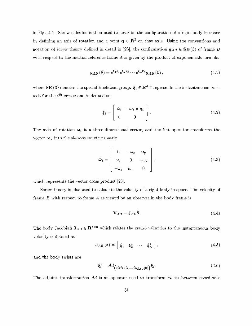
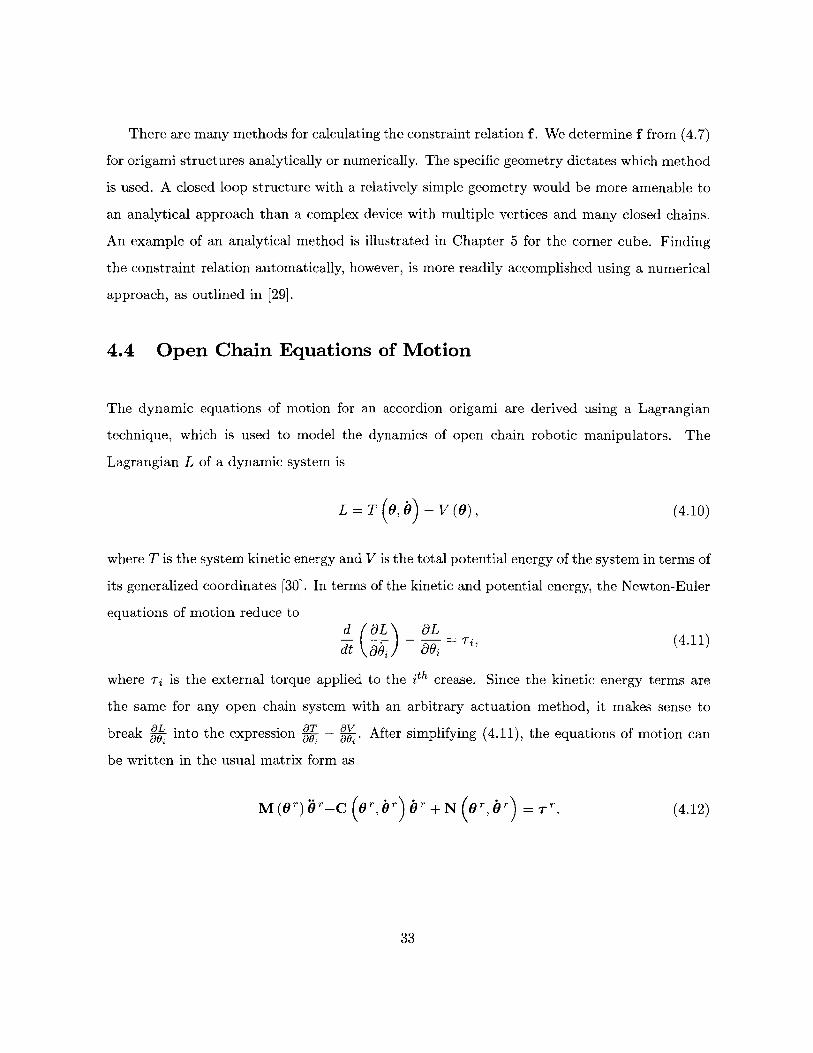
shown below in the OpenGL renderings. Fig. 3-3 shows the unfolding path of a piece of paper
folded in half once. Fig. 3-4 depicts the unfolding of the corner cube origami, while Fig. 3-5
illustrates the trajectory of the water-bomb base.
One main result of interest is that origamis whose crease pattern is symmetric folded quite
smoothly, but the asymmetric corner cube experienced local minima during the numerical min-
imization. Also, the fourth order energy function generates the smoothest unfolding trajectory.
The fourth order term induces a steeper energy gradient and creates a smooth, non-oscillating
trajectory.
25
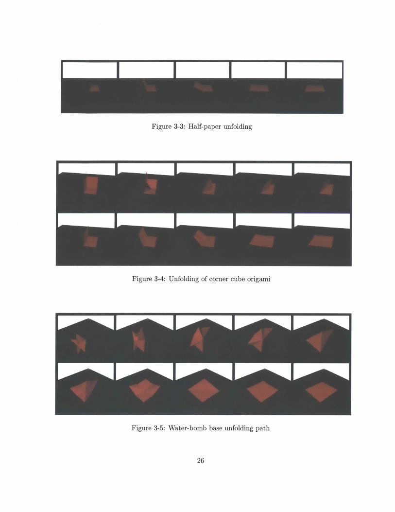
Figure 3-3: Half-paper unfolding
L ILI I
Figure 3-4: Unfolding of corner cube origami
Figure 3-5: Water-bomb base unfolding path
26

We have shown that energy methods can be used to unfold single-vertex origamis, but the
unfoldability of multiple-vertex origamis remains an open question. Perhaps similar methods
can be used to understand the kinematics of these complex structures. The discussion in
Chapter 6 will investigate possible avenues from which to approach this problem.
27

Chapter 4
Folding Dynamics
Modeling the dynamics of the actuation of Nanostructured Origami is essential to the suc-
cessful and repeatable manufacturing of nanopatterned origamis, just as analytical modeling
has streamlined the design of complex engineering systems such as integrated circuits and air-
craft. The scalability of Nanostructured Origami is limited by our understanding of arbitrary
geometries and of the dynamics of the actuation mechanisms. This thesis presents introduc-
tory research into the kinematic and dynamic modeling of accordion and single-vertex origami
structures.
The dynamics of actuating nanopatterned origamis can be simulated based on methods
developed within the robotics community. Each origami segment is modeled as a rigid body,
and the creases are represented mathematically by revolute joints. Origami segments should
remain rigid in order to maintain device integrity, which means that a stiff, strong material
should be selected for the structural membrane. Since the creases allow only one rotational
degree of freedom (DOF), the revolute joint model completely describes the relative motion of
the segments. Screw calculus is then used to parameterize the motion of each segment's center
of mass with respect to an inertial frame of reference. The equations of motion are formed
using the relevant material properties, kinematics, and constraints, from which the trajectory
is computed.
28

z(09, Fixed End
zX
B q3
Figure 4-1: Schematic of n-link accordion origami.
4.1 Origami Topology
Origamis are folded about pre-defined axes called creases that are created within the material
prior to folding. When folding paper, the creases are made simply by deforming the paper
in the desired locations. For Nanostructured Origami, the creases are defined with a specific
actuation method in mind. An accordion origami consists of a series of segments with the first
link connected to ground and the last link free. If there are n 1-DOF creases, then the origami
has n degrees of freedom. Fig. 4-1 shows the model for an accordion origami.
Many origamis, however, contain one or more closed kinematic chains. If the first and last
links of an origami have a common ground, then that origami has a closed kinematic chain,
or closed loop, topology. For these origamis, the number of degrees of freedom is not obvious
since many creases may intersect. The closed loop nature of origami introduces dependencies
between creases. Rotating one crease may produce rotations in several other creases, effectively
creating a kinematic constraint condition on its configuration. An example of a closed chain,
single vertex origami is shown in Fig. 4-2. The closed chain begins at A and loops around
through Crease n + 1 until the loop is closed again at A.
Another measure that is used to classify origamis is the number of interior vertices con-
tained within the initially flat origami. A vertex is the point at which creases intersect. A
29

B
On+1 8
%% 0
A
Figure 4-2: Schematic of arbitrary single-vertex origami
device with multiple vertices is more complex than one with a single interior vertex since there
are dependencies not only between creases in the local kinematic chain but also between neigh-
boring kinematic chains [21]. The most general Nanostructured Origami displays a closed loop
topology, has multiple interior vertices, and contains segments of various shapes. This thesis
calculates the dynamics of a set of rigid, closed chain origamis with only one interior vertex
and one closed chain, such as the corner cube. Formulating the dynamic equations of motion
for single vertex origamis is similar to the methods used for the accordions, but constraints
must be introduced to account for the closed kinematic chain. These results can then be used
as a basis for modeling more complicated structures with multiple vertices and several closed
kinematic loops.
4.2 Kinematics
Consider an accordion origami with n creases and n links as shown in Fig. 4-1, and attach an
inertial frame of reference A at the base of the origami and a body frame B at the center of
mass of the n'h link. An accordion origami with n creases can be parameterized in terms of
the crease angle Oi between the ith segment and the plane of the (i _ 1)th segment as shown
30
in Fig. 4-1. Screw calculus is then used to describe the configuration of a rigid body in space
by defining an axis of rotation and a point q E R3 on that axis. Using the conventions and
notation of screw theory defined in detail in [23], the configuration gAB E SE (3) of frame B
with respect to the inertial reference frame A is given by the product of exponentials formula
gAB (9) = e&1Ole4202 ... e4nngAB (0), (4.1)
where SE (3) denotes the special Euclidean group. j E R4X4 represents the instantaneous twist
axis for the ith crease and is defined as
c27 -wi x qigi[= (4.2)
0 0
The axis of rotation wi is a three-dimensional vector, and the hat operator transforms the
vector L o into the skew-symmetric matrix
0 -w wY
LL z 0 -. , (4.3)
W 0Y W'Lx 0
which represents the vector cross product [23].
Screw theory is also used to calculate the velocity of a rigid body in space. The velocity of
frame B with respect to frame A as viewed by an observer in the body frame is
VAB = JAB 0 - (4.4)
The body Jacobian JAB E R6 xn which relates the crease velocities to the instantaneous body
velocity is defined as
J AB (0) = *{ . *, 45
and the body twists are
= Ad(eioie e ... e )ngA(O )i. (4.6)
The adjoint transformation Ad is an operator used to transform twists between coordinate
31

frames [23].
For a closed kinematic chain, the loop is cut such that there are two open chains that meet
at a common coordinate frame B. Let frame B denote an "end-effector" located at the jth
segment of the origami as shown in the single vertex origami in Fig. 4-2. Chain 1 begins at
the base frame A and consists of creases i = 1 ... j. Chain 2 also begins at A but contains
Creases i = n + 1, n, - - j + 1. The loop equation for rigid origamis is given by the product of
exponentials formula as
e 10 1 ... e^A'gAB (0) = e n+10+1 ... A$+10j+1gA (0). (4.7)
This also introduces a constraint on the crease velocities for the two chains of the form
VAB 1(4.8)I 0 J2
where I is the identity matrix and Ji is the Jacobian for the ith chain [23].
4.3 Constraints
The rigidity condition imposes constraints on the crease angles of closed chain origamis that
must be included in the dynamic formulation. In general, an origami has N = n - m degrees
of freedom, where n is the number of creases and m is the number of holonomic constraints.
Since the number of creases is typically greater than the number of degrees of freedom, only N
creases need to be actuated by an external force, and m creases are simply passive creases in
the origami. Consider a single vertex origami with (n + 1) creases and segments as shown in
the 2-D crease pattern of Fig. 4-2. After virtually cutting one of the unactuated creases, the
reduced system, or the virtual open chain, now has the form of an accordion origami with n
generalized coordinates Oj, i = 1 ... n. Let 0' E Rn represent the crease vector for the reduced
open loop system. The n-dimensional vector of reduced system coordinates 0 ' is related to the
closed chain system coordinates 6 C E RN by the holonomic constraint equation [23]
or = f (0c) . (4.9)
32
There are many methods for calculating the constraint relation f. We determine f from (4.7)
for origami structures analytically or numerically. The specific geometry dictates which method
is used. A closed loop structure with a relatively simple geometry would be more amenable to
an analytical approach than a complex device with multiple vertices and many closed chains.
An example of an analytical method is illustrated in Chapter 5 for the corner cube. Finding
the constraint relation automatically, however, is more readily accomplished using a numerical
approach, as outlined in [29].
4.4 Open Chain Equations of Motion
The dynamic equations of motion for an accordion origami are derived using a Lagrangian
technique, which is used to model the dynamics of open chain robotic manipulators. The
Lagrangian L of a dynamic system is
L = T (,) -V (), (4.10)
where T is the system kinetic energy and V is the total potential energy of the system in terms of
its generalized coordinates [30]. In terms of the kinetic and potential energy, the Newton-Euler
equations of motion reduce to
= ri, (4.11)dt 00i a0z
where ri is the external torque applied to the ith crease. Since the kinetic energy terms are
the same for any open chain system with an arbitrary actuation method, it makes sense to
break aL into the expression V - . After simplifying (4.11), the equations of motion can
be written in the usual matrix form as
M (or) 6r+C ( , r)br + N (0 , r =rr. (4.12)
33

From [23], the inertia matrix M E R"xn and Coriolis matrix C E R"xn arise from -'d&Jab a~i
since V is independent of bi. M and C are defined as
n
M (0) = JT (0),<bJ, (0) (4.13)i=1
and
(0 ) 1 n + 19Mik cMk) =k,2 8 ao,0 80,- k=1 k j ai
where <k is the 6 x 6 inertia tensor given in [23]. -r' is the external torque vector applied to
the generalized coordinates 0 r.
The N (0, b) term on the left hand side of (4.12) includes generalized forces arising from the
potential energy of the system as well as any non-conservative forces applied at the creases. In
general, the potential energy of an origami is dependent on the strain energy in the hinges due
to bending and can also be considered independent of the actuation method used. Of course,
gravity should be included in the potential energy term, but simple calculations demonstrate
that the strain energy due to bending a segment through an angle 0 is orders of magnitude
higher than the work done by gravity on such small masses. As an approximation, the bending
is assumed to behave according to linear elastic deformation theory, which matches experimental
results of at least one actuation method [11]. The elastic strain energy of a hinge is defined as
potential energy of the form
V = 2z+0,y+ + +-2, - 2- (g-)+2 (1 + ii) (+ + + ]
(4.14)
where o-i is the ij component of the stress tensor, v is the Poisson ratio, E is Young's modulus,
and y is the volume of the hinge [31]. In many instances, the expression for strain energy
reduces significantly based on certain assumptions about the folding, and the bending mostly
occurs about one axis. In [11], for example, the plane stress assumption reduced the bending
equation to a one-dimensional problem as expected. For n hinges, the external moment vector
N (0, b) E Rn is related to the folding angle by the bending stiffness matrix K E Rnxn by the
34

relationship
N (0', r) = a + rc = KO + rnc, (4.15)
where -rc is a vector of non-conservative forces applied to the creases. The strain in one crease
is independent of the strain in another since the crease motions are independent, meaning that
K is diagonal.
4.5 Closed Chain Equations of Motion
Following the research presented in [23],[27], and others as described in Chapter 2, we convert
the closed chain origami into the original system and a reduced virtual open chain system.
We define the closed chain torque vector T c E RN and the reduced open chain torque vector
., r E Rn. The reduced system is assumed to undergo the same motions as the closed chain
system, meaning that
6WC = 6W', (4.16)
or
r -60c = -r . 60r
Thus, the virtual work is equivalent for both systems since they undergo the same motions
under the assumption of workless constraints. The differential form of (4.9) is
br = G6c (4.17)
or
60 r= G0 C.
The velocity constraint matrix G E RmxN that relates the open and closed chain virtual dis-
placements is defined as
OfG= Of(4.18)
Expression (4.12) represents the system's equations of motion for the reduced open chain
35

origami, and the torques are related by substituting (4.17) into (4.16) [28]
r C = GTr r. (4.19)
The reduced system equations of motion must be modified to account for the constraints so
that the resulting dynamics represent the actual motion of the origami. Using the relationships
in (4.19) and br = GOC, the closed chain equations of motion from [28] become
T C = GT[M (f (O C)) (G6cC + C) + C (f (0 C) , Gb ) Gc + N (f ( c) , G c)]. (4.20)
36

Chapter 5
Examples
5.1 Accordion Origami
5.1.1 Geometry
The accordion origami is the simplest topological classification of origami. Potential applica-
tions of accordion-type Nanostructured Origamis include layered devices such as 3D photonic
crystals [3] and bridge structures that are described in this example. A working electrochemical
supercapacitor, which was built with an accordion topology, was successfully fabricated using
Nanostructured Origami [7].
Although the equations defined in Chapter 4 are for any arbitrary actuation method, this
example models the external forces and hinges used in the stress-based actuation method. In
this procedure, a stressed material, such as chromium, is deposited on a relatively stress-free
structural layer of silicon nitride. After the device is released from the substrate, the stressed
material causes the structure to fold until the bending moment in the crease balances the
moment caused by the initial stress. The radius of curvature p of the hinge is calculated as
a function of material properties, geometry, and the initial stress in the material. Under the
assumptions of linear deformation theory, the length 14 of the ith hinge should be designed
according to the simple kinematic relationship 1i = pi~O, where 0 is again the turn angle of
the segment [11]. Fig. 5-1 illustrates experimental results obtained from the stress actuation
method. The three devices shown have an open kinematic chain topology with two hinges and
37

Figure 5-1: Accordion origamis actuated using a stressed bilayer.
two segments.
Consider the accordion origami crease pattern in Fig. 5-2a. This is a bridge-type structure
which is commonly used in MEMS devices.
For example, in [32] the bridge was actuated vertically by electrostatic means to modulate
the optical absorption in an underlying integrated optical circuit implementing a reconfigurable
add-drop optical switch. Bridges such as this are usually manufactured by etching away a
sacrificial layer; with the origami approach, a bridge could be manufactured according to the
schematic in Fig. 5-2b. There are four creases and segments to be folded, and the creases and
flaps are numbered consecutively from the base frame A. The axis of rotation wi and the point
38
- --- . . 0 0- Y -4?4 - I - - -

y w
-0 (a)
Kx
(b)
Figure 5-2: (a) Crease pattern of bridge device and (b) the bridge in its folded state.
39

on the axis qi in microns are defined as
1 = W2 =W3 = 4 = [0 (5.1)
0
0 0 0 0
qi = 0 ,2 L, q3 L, + L2 4 L, + L2 + L3 (5.2)
0 0 0 0
5.1.2 Equations of Motion
Following the general formulation outlined in Chapter 4, the open chain equations of motion
can be defined according to (4.12), where C and M are both defined in (4.13). The generalized
coordinates are shown in Fig. 5-1, and the vector representing these coordinates is
01
0r = 02 (5.3)03
04
The values of Ji (0), M (6), and C (0, e) are defined in detail in Appendix A.
Consider the membrane bilayer shown in Fig. 5-3. Layer 1 is the structural layer, while
layer 2 is pre-stressed.Of course, the Lagrangian could be computed such that the initial stress
is included in the potential energy term, but, in order to maintain full generality, the stress
will instead be included as an external torque term. The stiffness matrix K is then a diagonal
matrix representing the bending stiffness of each hinge. In this example, all four creases are
actuated, therefore each hinge is a bilayer. Based on the geometric assumptions in [11] with
the additional condition of zero initial stress, the uni-axial stress distribution in layer j due to
bending isZ
o-x,j =E -. (5.4)P
Ejis related to the elastic modulus Ej by E' 1 ) Now the potential energy in the hinge
40

Silicon nitridestructural layer
z
Stressed chromium layer
x
Figure 5-3: Diagram of thin film bilayer used in stress actuation technique.
can be calculated by substituting (5.4) into (4.14). The resulting expression
Vi = 2E 11/ (Ei) dI, (5.5)
represents the energy stored in a hinge due to bending. Substituting the kinematic relationship
1i = pi0 into (5.6), the resulting torque vector rbending - a is obtained as
Tbending = KO r, (5.6)
wherewt3E1 wt3E2K1 = K22 = K33 = K44 = 1 + 2 (5.7)
31 (1 - V2) 31 (1 - V()7
for the bilayer hinges, and w denotes the width of the hinges.
A non-conservative drag force B (0, b) is also included in the equations of motion to
model damping due to the origami's motion through air. The drag force is given by Fi =
}JCDOirA|V1 2 sgn(V where CD, ,ir, A, and 6, represent the drag coefficient, air den-
sity, surface area and surface normal, respectively, and sgn is the signum function. Thus, Fj
is the drag force applied at the ith body's center of mass in the direction opposite that of the
41

body's velocity. This force is projected along the direction of the generalized force vector by
= JfF1 + + F2 + F3+ 4F4 , (5.8)
where J, is the body Jacobian of the ith segment. The material properties and geometric
parameters used in the stress actuation procedure are shown in Appendix A.
5.1.3 Forward Dynamics
Step Input
Upon deriving the equations of motion, the forward dynamics for an arbitrary input force can
be simulated by numerically solving this second-order system of differential equations. For any
actuation method applied to an origami, the step response describes the system's response to
the immediate application of a set of generalized forces. Mathematically, this is represented by
solving (4.12) for the input torque at steady state as
7r/2
r = KO, = K 7r/2 (5.9)7r/2
Lr/2
for the device shown in Fig. 5-2. Within the context of the stress actuation method, the step
input represents the immediate release of the structural layer during the etch process.
We simulated the bridge origami using the material properties and geometry shown in
Table 1 of Appendix A. The bilayer is composed of a structural silicon nitride membrane and
the stressed chromium film. Since the sole source of damping in our model is drag, the system
is underdamped. The segment trajectories overshoot and quickly collide. The trajectories of
the segments as functions of time up to the first collision are shown in Fig. 5-4.
This result indicates that the instantaneous release is undesirable for this origami structure.
Instead, in the next section, we consider a ramp model of gradual release which overcomes this
problem.
42

Step Response for Angle I Step Response for Angle 2
-Thes1 The2
/
Oh>
41 003, 001 015 0 U2 /003 CO5 03 L.03 03
_6"
Step Response for Angle 3
10C0
'0 SO
20~~ ~ j/Oa101 O W 0u U04
Step Response for Ange 4
0006 O'Ot o is 0 5 U02 a p25 00 0 0 U . 001 p00 s i 002aM 003 5 004 0045
Figure 5-4: Step response of bridge device until collision.
Ramp Input
In practice, the release process is not immediate. Rather, the etch process occurs over a finite
time period. For example, in [11], the devices were released using a potassium hydroxide (KOH)
etch procedure. This highly directional etchant gradually releases the device from the silicon
substrate as shown in the schematic of Fig. 5-5. Other methods of releasing the devices (such
as UV or thermally-curable polyimides) might provide a faster actuation procedure, but the
etch is still not immediate. The exact shape of the actuation waveform is not known for most
cases. For the KOH etching, it can be modeled as a ramp, as we discuss in the remainder of
this section. For other actuation methods, the ramp response calculation described here can
still be useful, but it should be treated as an estimate only.
Consider the KOH etch process with etch rate ai for the ith hinge in the direction shown in
Fig. 5-5. Since the etch in this case is along the length 1i of the ith hinge, ai = L represents
the rate at which the hinge is released. By differentiating the kinematic constraint 1i = p6t, we
arrive atdlid= = Poi. (5.10)
43
U

KOH etch trench
I IChromium Silicon nitride
Figure 5-5: Schematic of KOH etch of single segment.
44

We can then integrate (5.10) to find Oi by
tSa !at t<t
Ot'ramp - dt = P(5.11)P hi t> t0 P P
where t, = poi,o/a is the time to completely underetch the hinge area of the origami. For
the KOH etch procedure in [11], the release occurs over a timespan of several hours since
a = 1.5pum/ min. The mathematical model for a ramp input is
r = C (Oramp, &ramp) bramp + B (Oramp, &ramp) + Keramp, (5.12)
where 6ramp and 0
ramp represent the vector describing the kinematics of the ramp input for
the KOH etch procedure. Solution of (5.12) over the time interval of 30 minutes leads to the
response plots shown in Fig. 5-6. Fig. 5-7 illustrates the trajectory of the bridge device as it
folds. Since there is no overshoot in Fig. 5-6, these results also indicate that there is no risk
of collisions for this particular device when using the KOH etch. If other release methods are
to be used in conjunction with the stress actuation method, then it is necessary to develop a
suitable model of the release process and incorporate that into the input torque formulation.
5.1.4 Stability
After the folding operation has been completed, another important consideration is the stability
of the device in its final configuration. For these devices, the equilibrium position is given by
7r/2
7/26 eq = / . (5.13)
Lr/2
- r/2-
In the simulations above, we used the value of p predicted in [11] based on the material
properties of the chosen material system of SiN,-Cr hinges. In equilibrium, Oi = li/p, so the
desired equilibrium angles (5.13) can be guaranteed by properly selecting the hinge lengths.
Moreover, since from (5.9) it can be seen that K is a positive definite matrix, the equilibrium
45

Rarrp Response for Angle 1100
0 1 1 20 2 3
80n epos o Age3
70 0 5 2 2 060 mi)
Figure 5-6: Ramp response plots for bridge device.
Time: 0 min
Time: 14min
Figure 5-7: Trajectory of bridge resulting from ramp input.
46
III
II
Ramp Response for Angle 2
80- -
0 5 1 5 2 5
Ranp Response for Angle 4
I
I s1 )TWMe "n)
Time: 7 min
Time: 21 min
I
0 20 25 ju

is guaranteed to be stable.
We now proceed to evaluate the natural frequencies of the linearized system. Consider the
steady state configuration of the bridge as shown in Fig. 5-2b. The linearized equations of
motion are given by
A6 + M KAO = 0, (5.14)
where A6 is the generalized displacement from equilibrium. The eigenvalues and eigenvectors
of the folded system are of particular interest for control systems designed to maintain the final
configuration. The eigenvalues of the positive definite matrix A = M- 1 K are
4.50 0 0 0
A=10 12 0 0.32 0 0 (5.15)0 0 0.064 0
0 0 0 0.0024
and the eigenvectors are the columns of the matrix
0.0127 -0.1983 0.9495 -1.0000
-0.0204 0.2082 -1.0000 -0.9496V = .(5.16)
0.0870 -1.0000 -0.3962 -0.00002
-1.0000 -0.0937 -0.0020 0.0067
The natural frequencies are found from (5.15) and are 337.6 kHz, 90 kHz, 40.4 kHz, and 7.88
kHz for the four modes of vibration. These frequencies are high in magnitude as expected
since the masses of the membranes are very small compared to the crease stiffnesses. This is
advantageous because the device will be robust to slow perturbations.
5.2 Corner Cube Origami
5.2.1 Geometry
The corner cube is a single vertex origami that is well-known within the origami mathematics
community. It has been studied by [21] because it is one of few known origamis that can fold
47

Virtually cut joint0
xx
0, 0' 0
(a) (b
Figure 5-8: Schematic of (a) original closed chain corner cube and (b) reduced open chainsystem
rigidly. Besides being a mathematically interesting device, the corner cube is a useful optical
device because it acts as a retroreflector to incident light.
The crease pattern of the corner cube is shown in Fig. 5-8a. In this figure, the closed chain
is represented by the generalized coordinate vector 0= 01 02 03 04 05 This para-
meterization of the corner cube, however, is not an independent set of generalized coordinates
since the closed chain introduces kinematic constraints between the crease angles. Following the
formulation defined in Chapter 4, the N degree of freedom closed chain system of Fig. 5-8a is
converted into an equivalent virtual open chain by cutting the structure at Crease 5, which we
select to be unactuated. Fig. 5-8b illustrates the virtual open chain system with n generalized
coordinates defined by 0' = [01 02 03 04 1
The number of degrees of freedom N of a general spatial mechanism can be determined by
the Grubler-Kutzbach criterion [33]
PN = 6 (r -p - 1) + fi, (5.17)
i=1l
where r is the number of rigid links, p is the number of creases, and fi represents the number
of degrees of freedom of the ith crease. For the corner cube, (5.17) reduces to
5
N = 6 (5 - 5 - 1) + T1 = -1. (5.18)
48

The negative result in this case indicates that this origami is overdetermined [33],[22]. If one axis
of rotation is locked, however, then the system is effectively converted into the familiar 1-DOF
4R overconstrained system that is well-understood in the robotics community [22]. Blocking
the rotation axes in this manner naturally allows for a two-step actuation sequence:
Step 1 - Lock 02 and fold the 4R overconstrained subsystem 180' about 01
Step 2 - Lock 01 and fold the partially-folded origami 90 about 02.
Therefore, the corner cube can be modeled as a 2-DOF system described by 01 and 02 in
which each degree of freedom is actuated in a separate step. For the stress actuation method,
this implies that only Creases 1 and 2 require the stressed bilayer for actuation. The other
three creases will be passive hinges that are kinematically dependent on the driving angles 9 C.
In the folding motion of Step 1, N = 1 since this is a 4R overconstrained system. Because
02 is locked during the first folding sequence, the reduced open chain coordinates are described
by r =[ 01 03 04 ]. Upon choosing 0' = [011T to be the independent generalized coordi-
nate vector of the original closed chain system, it is evident that there are m = 2 holonomic
constraints relating 6' to 6 C by (4.9).
Previous work [22] determined the holonomic constraint relation for the corner cube. Those
results are briefly illustrated in Chapter 2. The constraint f is calculated by a virtual cut at
Crease 5 for the first fold. The two kinematic chains stemming from the base frame A and
resulting from the cut have an open chain topology. Crease 1 from the first chain is the input
angle which is perturbed by a known angle, and the configuration of the end effector at Crease
5 is computed using (4.1).
The inverse kinematics chain also begins at Crease 1 but traverses the opposite direction
through Creases 2, 3, and 4. (4.7) is used to solve the inverse kinematics problem to find
the change in the output angles 03 and 04 due to the perturbation at 01. The input-output
relationship that is found from the loop closure equations allows for the determination of f in
(5.19) which is described graphically in Fig. 5-9. Although an expression relating 6' and 6 C is
generally difficult to determine analytically, a fourth order polynomial curve fitting technique
was employed to obtain an approximate analytical relationship between the coordinates in
49

Kinematic Constraints for Corner Cube
0 20 40 60 80 100 120 140
Thetal (deg)
Figure 5-9: Holonomic constraint relation for corner cube
degrees given by [22]
[01103
04
0r = f (0C);
- 1 04 +
a4 104 +
(5.19)
a3203 + a33 02 + a34 01 + a35
a420- + a430- + a4401 + a45 Iwhere the constant coefficients are found in Table 2.
a3k (deg) a4k (deg)
k = 1 -1.8 (10-8) -2.4 (10-8)
k = 2 -3 (10-6) 1.2 (10-5)
k = 3 3.1 (10-5) -6.2 (10-4)
k = 4 0.71 0.37
k = 5 0.0089 -0.015
Table 2. Polynomial coefficients for constraint relations
To parameterize the corner cube using screw calculus, the twist axes and the points on those
axes must be defined as described in Chapter 4. For the device in Fig. 5-8b, wo and qj (in
50
90
75
0
45
30
is
160 180
................ .............. --------------- ........... - -------------------------------------------------------

microns) are given by
-1 1 0
1i = [1 W3= 0 ,W4= 1 (5.20)
0 0 0
and
0 L L/2
q = 0 ,3 L/2 q4 L
0 0 0
5.2.2 Equations of Motion
Consider the virtual open chain origami of Fig. 5-8b. In this reduced system, each angle of
0' is modeled as having a virtual actuator attached to every crease. The equations of motion
for this open kinematic chain are given by (4.12), where M and C are still defined by (4.13).
The values for the reduced system matrices Ji, M, and C are given in Appendix B. Similarly,
= J1 + J3 F3 + J F4 , and the stiffness matrix K is a 3x3 diagonal matrix with entries
Kij defined by
wt! E1 wt|E2Ki1 = ( + 2 , (5.21)31 (1 - v) 31, (1 - vl)(
K 22 = K 33 = (11 2.312 - v1)
Because creases 3 and 4 are unactuated, the length 12 of the unstressed hinges can be set
arbitrarily to minimize the radius of curvature of the creases. The dynamics of the virtual
open chain, in terms of 0', is described precisely by this system of three ordinary differential
equations originally presented in (4.12).
51

5.2.3 Forward Dynamics
Step Input
In order to simulate the dynamics of the corner cube, it is first necessary to calculate the input
generalized torque r' E R xl applied to Crease 1 as outlined in [261,[27]. The reduced system
virtual torque -r E R3 x1 is determined by
r K = K [r/2 (5.22)
7r/2
for a step input with virtual actuators attached to Creases 3 and 4. (5.22) represents the virtual
open chain dyamics, but the open chain parameterization does not account for the closed loop
constraints. The closed chain input torque r' is related to r by the constraint Jacobian
G E R 3x1 by
T = GTr , (5.23)
7" = 190 Q04 ao r,8O1 8d1 ]'~where the partial derivatives in GT can be found simply from the quartic holonomic constraints
in f.
Let l denote the longer hinge length associated with the closed chain such that the com-
pliance of the crease results in the requisite amount of torque. One way to determine lU is to
use a concept of "torque magnification", which describes the magnification on the open chain
torque that is required to actuate the closed chain. Let 7- and 7' be the torques required to
actuate Crease 1 of the virtual open chain and the closed chain systems, respectively. Then,
we define the torque magnification factor ?7 as
= -. (5.24)
52

S
.20,C4
180
160
140
120
100
80
60
40
20
0
Step Response for Angle 1
0 0.00001 0.00002 0.00003 0.00004 0.00005
Time (s)
Figure 5-10: Step response of corner cube until collision.
This value can be used to approximate the new value of the stiffness kI for Crease 1 as
ki - (5.25)7)
Finally, the longer hinge length lU can be found from (5.7). This value is then substituted into
the equations of motion (4.20).
The geometric parameters for the corner cube used in this simulation are shown in Table
3 of Appendix B. Fig. 5-10 plots the step response of Crease 1 until collision for the corner
cube origami resulting from the input torque T c. Again, the response plots show that collisions
occur, which indicates that a ramp input model is more accurate. The preceding discussion
describes the dynamics of actuating Step 1 of the actuation sequence. Since 03, 94, and the cut
angle 05 have reached the folded state, the resulting partially folded origami has 1-DOF about
02 which can be easily modeled without constraints according to the analysis above..
5.2.4 Ramp Input
Following the arguments above regarding etch rates, a more accurate input torque model
53

Ramp Response of Joint I
180
180
140
120
100-
80
60
40
20
0 10 20 30 40 50
Time (min)
Figure 5-11: Ramp response of corner cube
for the stress actuation technique is defined by a ramp
kinematic chain, this is expressed as
input to the active creases. For a closed
''= GT r = GT (C (6ramp, bramp) bramp + B (6ramp, bramp) + K~ramp . (5.26)
The response plots are illustrated in Fig. 5-11, and a schematic of the folding of the corner cube
can be seen in Fig. 5-12. The first three plots illustrate the motions for Step 1, while the last
shows the final folding motion of Step 2. The response exhibits minimal overshoot compared to
the step response. This indicates that the ramp input model for the stress actuation procedure
predicts no risk of serious collisions between the segments.
54
0
a,C4

0 min
475 m
23.8 min
Step 2 fold
Figure 5-12: Trajectory of corner cube resulting from a ramp input.
5.2.5 Stability
The final folded configuration of the corner cube is shown in Fig. 5-12, where the equilibrium
crease angles of the closed chain are defined as
(5.27)
01 7r
02 7/26
eq = = ./03 7r/2
04 7r/2j
The folded configuration has 2-DOF with 01 and 02 again as the generalized coordinates of the
device. (4.20) is linearized about the equilibrium point subject to the constraints of (5.19) since
small motions about equilibrium must still obey the constraints. The nonlinear drag force is
again neglected at equilibrium in the equations of motion, and the Coriolis matrix disappears
as described in detail in [30]. The resulting system of two differential equations is
A'+M--KAOC= 0. (5.28)
55
The eigenvalues are given by
A = 109 0.29 0 , (5.29)0 3.3
while the associated eigenvectors are the columns of
-0.986 0.35
L -0.166 -0.94 (
The natural frequencies are given by 2.7 kHz and 9.1 kHz.
Since the stiffness matrix is positive definite, the corner cube is indeed at a stable equi-
librium. In fact, one of the principle benefits of the stress actuation method is that the final
folded state will always be at a stable equilibrium since the stiffness matrix is always a square,
positive, diagonal matrix. The inherent mechanics of the process ensure that the torque due to
the stressed membrane is always stably balanced by the bending moment.
56

Chapter 6
Conclusions and Future Work
This thesis presents modeling techniques that can be used to simulate the actuation of Nanos-
tructured Origami devices. The analytical methods are based on the large body of information
available on origami mathematics and robotics. The primary achievements relate to the geom-
etry and physics of the folding and unfolding of single-vertex and accordion origamis. It is
expected that this research will lay the foundation for the simulation of more complex origamis.
6.1 Single-Vertex Unfolding
The rigid unfolding of single-vertex origamis has been demonstrated. The unfolding trajectories
of the half-paper, corner cube, and waterbomb base were simulated using energy methods
that were previously explored in [15]. A constrained optimization routine was implemented
to calculate the trajectories numerically, and the kinematic constraints can then be extracted
from the results. The direct extension of energy methods to the unfolding and kinematics of
multiple vertex origamis is unknown, but it presents interesting research questions to pursue.
6.2 Simulation of Origami Dynamics
A generic formulation for modeling the dynamics of Nanostructured Origami has been pre-
sented based on techniques that are widely used to model robotic manipulators. We extend
these methods to model origamis with open kinematic chains and those containing one closed
57
kinematic chain (i.e. a single interior vertex). The input generalized forces necessary to actuate
the origamis were calculated, and the forward dynamics were simulated for both a generic ac-
tuation method and for the stress actuation procedure. The response of a ramp input for both
types of origamis is very-well behaved, as there is no overshoot due to the slow etching rate.
For stress actuation, it was also verified that since the stiffness matrix is always positive definite
at an equilibrium position, the final folded configuration is stable. The same principles can be
used to calculate the dynamics of origamis with multiple interior vertices and closed kinematic
chains, but determining the kinematic constraint relations will inevitably be more complex.
6.3 Future Work
Nanostructured Origami offers great promise as an effective 3D nanomanufacturing process.
Besides the theoretical investigations outlined in this thesis, several actuation mechanisms have
been successfully tested, and a working origami device [7 has been fabricated. Other researchers
in the 3D Optics group at MIT are actively investigating precision alignment techniques and
latching mechanisms that can be used to accurately position the devices in the folded state.
Thus, there are exciting directions in which we can further develop the technology.
From the theoretical front, the following modeling tools should be developed:
" Software suite - In order to expedite the design process for an arbitrary origami, the
modeling techniques described here should be implemented in an extensive software tool.
[22] developed a software tool using Visual Basic for simulating the corner cube. The
dynamic modeling capabilities are now being integrated with the kinematics in a new
software suite using Microsoft's C# language. When further theoretical developments
are made, they will also be added to the software so that the origami design process is
automated.
" Experimental verification - It is imperative that the dynamic models are tested in the lab
on folding origamis. Various types of sensors can be used to track the trajectory as the
origami folds, and the results will be compared to the analytical results.
" Control schemes - Theoretical and experimental control strategies should be explored in
58
order to make the actuation process more robust. Feedback will improve the plant model
of the actuation scheme, and the placement of the origami segments will be more accurate.
e Multiple vertex origamis - Little is known about the geometry of multiple vertex origamis.
The ultimate objective is to be able to transform a 3D design from the concept stage to a
working crease pattern for the Nanostructured Origami technique. Optimization routines
such as the energy method offer promising results for understanding these origamis. Per-
haps a similar method will help in solving the unfolding of rigid multiple vertex origamis.
Pseudo-triangulation is also a promising technique for investigating origamis with mul-
tiple vertices. The 1-DOF motion is an attractive strategy since the unfolding motion is
simplified considerably.
59

Part I
Appendix A: Geometric
Material Parameters for Bridge
60
and

Parameter Value Units
p 20 pm
1 32 pIm
w 100 pIm
ti 0.2 pm
t2 0.1 pim
E1 300 GPa
E2 140 GPa
V1 0.28
V2 0.21
Om 3.27E-12 g/am3
L, 100 pum
L2 400 ,um
L3 100 [Lm
L4 20 IamTable 1. Parameters for bridge devie
The Jacobians, mass and Coriolis matrices for the bridge origami are shown below. si and ci
represent sin and cos of the ith joint, and /m is the mass density of the silicon nitride structural
material.
0 0 0 0
0 0 0 0
L1/2 0 0 0
1 0 0 0
0 0 0 0
0 0 0 0
61

0
L1 s 2
L1 c2 +L 2 /2
1
0
0
0
LIs3 c2 + LIs 2c 3 + L 2s3
L1c 3c2 + L 2 c3 -
LIs 2s 3 + L 3 /2
1
0
0
column 1 of J 4 :
0
L2 83
L2 c3 +L 3 /2
1
0
0
0
c2 c4 s 3 L1 + c2 s 4 c3 L1+
s 2c4 c3 L1 + c4 s 3L 2 +
s4c3 L 2 - S2 s 4s 3 L1 + s4 L3
1/2L 4 + c4 L 3 + c2 c4 c3 L 1-
c2 S4 8 3 L1 - s2 c4 s3 L 1-
s2 s4 c3 L 1 + c4 c3 L2 - S4 s 3 L2
1
0
0
62
J2 =
0
0
L2 /2
1
0
0
0
0
0
0
0
0
0
0
0
0
0
0
J3 =
0
0
L3 /2
1
0
0
0
0
0
0
0
0

column 2 of J4 :
columns 3 and 4 of J4
0
c4 s3 L 2 + sc 3 L2
+s 4 L3
c4c3L2 + c4 L 3 +
1/2L4 - s4 s 3L 2
1
0
0
0
s4 L3
c4 L3 + 1/2L4
1
0
0
M -= 1/4L3 mWti + 1/120mLiw3t, + 1/123mLiWt3 +
1/12#mL 2Wt1(12L2 + 12Lic 2 L2 + 3L + W2 + t2) +
1/120mL3 wtI(24Lic 2 L2 + 12L 2 + 12c3 Lic 2 L3 +
12c3 L2 L3 + 12L2 - 12s 3 Lis 2 L3 + 3L + W 2 +
tj) + 1/123mL4 Wti(tl + W2 + 3L + 12L2 +
12L4c4 L3 + 12L2 + 24L1c 2L2 + 12L4c2c 4c3 L1
-12L 4c 2s 4s 3 L1 - 12L4 s2c4 s3 L1 - 12L4 s2 s4c 3 L1
+12L3 + 24c3 L 2L 3 + 24c3 Lic 2 L3 - 24s3Lis2 L 3
+12L 4c 4c 3 L2 - 12L 4 s4s 3L 2 )
63
0
0
L4 /2
1
0
0

M12= 1/12/3mL2Wti(6LiC 2 L 2 + 3L + I+ t) +
1/12/3mL 3Wti(12LiC 2 L2 + 12L2 + 6c3 Lic 2 L3 +
12c3 L 2L 3 - 6s3 Lis 2 L3 + 3 + + t1) +
1/12/mL4 Wt(-12S 3LIS 2 L3 + 12c3 Lic 2 L3 +
12LIc 2 L2 + tI + w2 + 3L4 + 24c3 L2 L3 + 12L2 +
12L4 c4 L3 + 6L 4c2c4 c3 L1 - 6L 4 c2 s4s 3 L1
-6L 4s 2c 4s 3L 1 - 6L4 s2 s4c 3 L1 + 12L4+
12L 4c4c3 L 2 - 12L4 s4 s3 L 2 )
M13= 1/120mL3Wti(6C3LiC2 L 3 + 6c3 L2 L3 - 6s3 LIs 2 L3
+3L + + t1) + 1/123mL4Wti(12C3 LiC2 L 3 +
12c3 L2 L3 - 12s3 Lis 2 L3 + 12L 2 + 12L4 c4 L3 + 3L
+6L 4c2 c4 c3 L1 - 6L4 c2 s4 s3 L1 - 6L4 s2 c4 s3 L1 -
6L4 s2 s4 c3 L1 + 6L4c4 c3 L 2 -6L 4 s4 s3 L m2 + W + t)
M14= 1/l2#mL4 Wt1(3L I + 6L4c4 L 3 + 6L4c2 c4c3 L1 -
6L4 c2 s4s 3L1 - 6L4 s2c 4s 3 L1 - 6L4 s2s 4c3 L1 +
6L4 c4 c3L2 - 6L4 s4 s3 L2 +W2 +t 2)
64

M21 1/12/3mL2 Wti(6LiC2 L 2 + 3L+2 +t) +
1/123mL 3Wti(12LiC 2 L2 + 12L2 + 6c 3Lic 2 L 3
+12c 3 L2 L3 - 6s3 L1s 2L 3 + 3L + W2 + t2)+
1/123mL 4Wti(-12s 3 Lis 2 L3 + 12c3 Lic 2 L3 +
12Lic 2 L2 + t2 + w2 + 3L + 24c3 L2 L 3 + 12L2
+12L 4c4 L3 + 6L4c 2c4 c3L1 - 6L4 c2s 4s3 L1 -
6L4s 2c4s3 L 1 - 6L4 s2s 4c3 L1 + 12L2 +
12L4c 4c3 L2 - 12L 4 s4s 3L 2 )
M22= 1/4L !3mWt1 + 1/12mL2W 3t1 +
1/120mL 2Wt3 + 1/123mL 3 Wti(12L2 +
12c3L 2 L 3 + 3L + t) + 1/12,3mL4Wti
(24c3 L2L3 + 12L2 + 12L4c4c3 L 2 - 12L4 c4 L3
+3L2 - 12L4 s4 s3L2 +12L + 2 + t )
M23= 1/12mL3Wti(6C3 L 2L 3 + 3Li + 2+ t) +
1/12QmL 4wtl(12C 3 L2 L3 + 12L2 + 6L4 c4c3L 2
+12L 4c4 L3 + 3L - 6L 4 s4 s3L2 +w2 + t2)
M24= 1/12/mL4 Wt1(6L 4C 4C3L 2 + 6L4 c4 L3 +
3L - 6L4 s4s 3 L2 w2 + )
65

M31= 1/1203mL 3Wti(6C3 LiC2 L3 + 6c3 L 2 L3 -
6s3 Lis 2 L3 + 3L + +t) + 1/12,BmL4 Wtl
(12c 3 Lic 2 L3 +12c 3 L 2 L3 - 12s 3 Lis2 L 3
+12L2 + 12L4c4 L3 + 3L + 6L4c 2c4c 3 L1
-6L 4c 2s 4s 3 L1 - 6L4s2c 4s 3 L1 - 6L4 s2 s4c 3 L1
+6L4c 4c 3 L2 - 6L4 s4 s3 L 2 + W 2 + t 2)
M 32 1/123mL3Wti(6C3 L2 L 3 + 3L +
I+ t) + 1/120,mL4Wti(12C 3 L 2 L3
+12L2 + 6L4c4 c3 L2 + 12L4c 4
L3 + 3L - 6L4 s4s 3 L2 + w 2 + t2)
M33 = 1/4L /3mWti + 1/120mL3W3 t
+1/123mL 3Wt3 + 1/123mL4Wti
(12L2 + 12L 4c4 L3 + 3L + W2 + t2)
M34 =1/12#mL4Wti(6L4C 4 L3 + 3L +W2 + t2)
66

M41= 1/12#mL 4 Wti(3L2 + 6L4c4 L3 +
6L4c 2c4c3 L1 - 6L4 c2 s4 s3 L1 -
6L4 s2c4 s3 L1 - 6L4 s2 s4c3 L1 +
6L4 c4c3 L 2 - 6L4 s4 s3 L2 +W2 + t2)
M42= 1/120,L4Wt1(6L 4C 4C3 L 2 + 6L4 c4 L3 -+
3Li -6L 4s4s3 L2 +W2 + t)
M43 = 1/12/mL4 Wt1(6L4C 4 L3 + 3L + W2 + t2)
M44 = 1/4L 3mWt1 + 1/12,3.L 4 W3t1 + 1/12OmL4Wt3
67
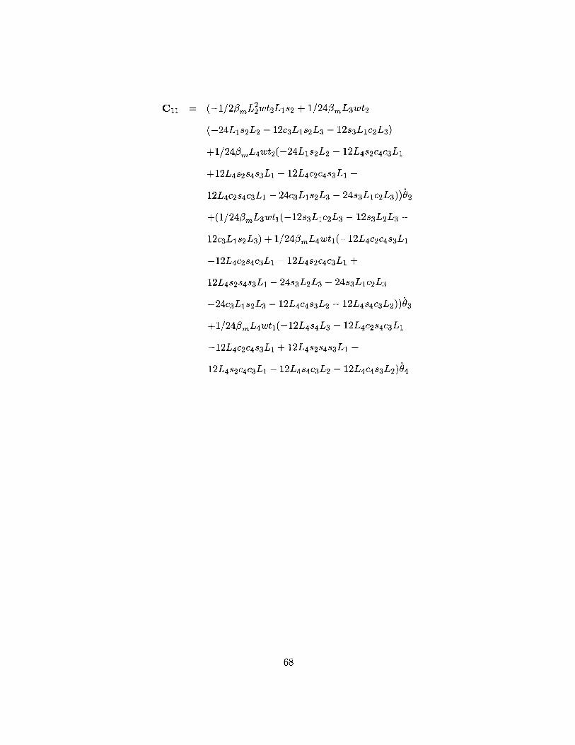
C2 (1/23mL t2LiS2 + 1/243mL3Wt2
(-24LIs 2L 2 - 12c3 LIs 2 L3 - 12s 3Lic 2L 3 )
+1/24,3L4Wt 2 (-24L1 s 2 L2 - 12L4 s2c 4c3 L1
+12L 4 s2S 4 s3 L1 - 12L4 c2c4 s3 L1 -
12L4 c2 s4 c3 L1 - 24c3 Lis 2L 3 - 24s3 Lic 2 L3 ))0 2
+(1/24,3mL 3Wti(-12s 3 LiC2 L 3 - 12s 3 L2 L3 -
12c3 Lis 2 L3 ) + 1/243mL 4Wti(-12L 4C 2C4 S3 LI
-12L 4c 2s 4c 3 L1 - 12L4 s2c4c 3 L1 +
12L4 s2 s4 s3 L -24s 3 L2 L3 - 24s 3 Lic 2 L3
-24c 3 Lis 2 L3 - 12L4c4 s3 L2 - 12L4 s4c3 L 2 ))03
+1/243mL 4Wti(-12L4s 4 L3 - 12L4c 2s 4c 3 L1
-12L 4c 2c 4s 3 L1 + 12L4 s2 s4s3 L1 -
12L4 s2c4 c3 L1 - 12L4 s4C3 L2 - 12L4 c4 s3 L2 )b4
68

C 12 = (-1/2mL2wtiLiS 2 + 1/243mL 3Wti
(-24LIs 2L 2 - 12c3 Lis 2 L3 - 12s3 Lic 2 L3 )
+1/24fmL 4 Wt1(-24L1s 2 L2 - 12L4s 2c4c 3L1
+12L 4s 2S 4s 3 L1 - 12L4c 2c4 s3 L1 -
12L4 c2s4c 3 L1 - 24c3Lis2 L3 - 24s 3 Lic 2 L 3 ))Ai
+(-1/2mL 2wtiLiS2 + 1/123mL 3Wti(-12Lis 2L 2
-6c 3 Lis 2L 3 - 6s3Lic 2L 3 ) + 1/12mL4Wtl
(-12s 3 Lic 2 L3 - 12c3 Lis 2 L3 - 12LIs 2L 2
-6L 4s 2c 4c 3 L1 + 6L 4 s 2s 4 s 3L1 - 6L4c2 c4 s3 L1
-6L 4c 2s 4c3 Li))b 2 + (1/240mL3Wtl(-6s 3 Lic 2 L3
-12s 3 L2 L3 - 6c3 Lis 2 L3 ) + 1/243mL4 Wti
(-12c 3 Lis 2L 3 - 12s3 Lic 2 L3 - 24s3 L2 L3 -
6L4 c2c4 s3 L1 - 6L4 c2 s4c 3L1 - 6L4s 2c4c 3Li
+6L 4 s2 s4 s3 Ll - 12L4 c4 s3 L2 - 12L4 s4 c3 L2 ) +
1/24omL3 Wti(-6 3 LIS 2 L3 - 6s 3Lic 2 L3) +
1/24#mL4 Wti(-12C3 LiS 2 L3 - 12s3 Lic 2 L3 -
6L 4s 2c4c3 L1 + 6L 4 s 2 S4s 3 L1 - 6L4c2 c4 s3 L1
-6L 4c 2s 4c 3 L1 ))b3 + (1/240mL4Wtl
(-12L4s 4 L3 -6L 4 c2 s4c3 L1 - 6L4c2 c4 s3 L1 +
6L4 s2s 4s3 L1 -6L 4 s2c4 c3 L1 -12L 4s4 c3 L 2 -
12L 4c4 s3 L2 ) + 1/240mL4Wtl(-6L 4S 2C4C3 Li
+6L 4s 2s4 s3L, - 6L4 c2 c4 s3L1 - 6L 4c2 s4 c3 L1 ))b 4
69

C 13 (1/243mL3 Wti(-12S 3 LiC2 L3 - 12s 3 L2 L3 -
12c3 Lis 2 L3 ) + 1/24!#mL4Wti(-12L 4C 2C4 S3 Li
-12L 4c 2s 4c3 L, - 12L4 s2c 4c3 L1 + 12L4 s2 S4s 3 L1
-24s 3L 2L 3 - 24s3Lic2 L3 - 24c3 Lis 2 L3 -
12L4 c4 s3L 2 - 12L4 s4 c3 L2 ))Oi + (1/243mL3Wtl
(-6s 3 Lic 2 L3 - 12s3 L 2 L3 - 6c 3 Lis 2 L3 ) +
1/24#3mL4 Wti(-12C 3 LS 2L 3 - 12s3 Lic 2 L3 -
24s3L 2 L3 - 6L4 c2 c4 s3 L1 - 6L4 c2s4 c3 L1 -
6L4s2c 4c3 L1 + 6L4 s 2s 4 s 3 L1 - 12L4 c4 s3 L 2 -
12L4 s4c3 L2 ) + 1/24I3mL3 Wtl(-6C3 LiS 2 L3
-6s 3 Lic 2 L3 ) + 1/24ImL4 Wt(-12 3 LIS 2 L3 -
12s3 LIc 2L3 - 6L 4s 2c4 c3 L1 + 6L4 s2 s4s 3 L1 -
6L4c 2c4 s3L1 - 6L4 c2 s4 c3 L1))0 2 + (1/123mL3Wt1
(-6s 3Lic 2 L3 - 6s 3 L2 L3 - 6c3 Lis 2 L3 ) +
1/12omL 4 Wti(-12 3 LC 2L 3 - 12s3 L2 L3 -
12c3 Lis 2 L3 - 6L4 c2c4 s3 L1 - 6L4c2 s4c 3L1
-6L 4s 2c 4c 3 L1 + 6L 4 s2 s4s 3 L1 - 6L4c4 s3 L 2 -
6L 4s4 c3 L2 ))0 3 + (1/240mL4 wtl(-12L4s 4 L3
-6L 4c 2s 4c 3L1 - 6L 4 c2c4 s3 L1 + 6L4 s2 s 4 S3 L1
-6L 4s 2c 4c 3L1 - 6L4 s4c3 L2 - 6L4 c4 s3 L 2 ) +
1/ 2 4 3 mL4Wtl(-6L 4c 2c4 s3 L1 - 6L4 c2 s4c3 L1
-6L 4s 2c 4c 3 L1 + 6L 4 s 2 s4s 3 L1 - 6L4 c4 s3 L2
-6L 4s 4c 3L 2 ))b4
70

C14 = 1/24/3mL4 Wt(-12L 4s 4 L3 - 12L4c2 s4 c3 L1
-12L 4c 2c 4s 3L1 + 12L4 s2 s4 s3 L1 -
12L4 s 2c 4c3 L1 - 12L 4 s4c 3L 2 - 12L4 c4 s3 L 2 )bl
+(1/24mL4 Wt(-12L 4s4L3 - 6L4 c2 s4c 3L1 -
6L4 c2c4 s3 L1 + 6L4 s2 s4 s3L1 - 6L4 s2 c4c 3 L1 -
12L4s 4c3 L2 - 12L4 c4 s3 L 2 ) + 1/243mL 4 Wtl
(-6L4s 2c 4 c3 Li + 6L 4 s 2 s4s 3 L1 - 6L4c2 c4 s3 L1
-6L 4c 2s 4c 3 L1))0 2 + (1/243mL4 Wt1(-12L4S4L3
-6L 4c 2s 4c 3Li - 6L4c 2c4 s3 L1 + 6L4 s 2s 4 s 3L1
-6L 4s2 c 4c 3 L1 - 6L4 s4c 3 L2 - 6L4 c4 s3 L2 ) +
1/240mL4Wtl(-6L4C2C4s3L1 - 6L4c2s4c 3L1
-6L 4s 2c 4c 3 L1 + 6L4 s2s 4s 3 L1 - 6L4 c4 s3 L 2 -
6L 4 s 4c3 L2 ))b 3 + 1/123mL4Wtl(-6L4s 4 L3 -
6L 4c2 s4c 3L1 - 6L4c 2c4 s3 L1 + 6L 4 s2 s4 s3 L1 -
6L4s2 c4 c3 L, - 6L4 s4c3 L 2 - 6L 4c4 s3 L 2 )04
71

C 2 1 (1/23mL2wtILiS 2 - 1/243mL3 Wt(-24LS 2 L 2
-12c 3 Lis 2 L3 - 12s3 Lic 2 L3 ) - 1/24#mL4
wt1(-24L1 s 2 L2 - 12L4 s 2c4c 3 L1 +
12L 4 s2 S4 s3 L1 - 12L4 c2c4 s3 L1 - 12L4c 2s4 c3 L1
-24c 3 Lis 2 L 3 - 24s3 Lic2 L3 ))9i + (1/243mL3Wti
(-6s 3 Lic 2 L3 - 12s3 L 2L 3 - 6c3 Lis 2 L3 ) +
1/243mL4Wti(-12c3Lis2 L3 - 12s 3 Lic 2 L 3 -
24s3 L2 L3 - 6L4c2c4 s3 L1 - 6L4 c2 s4c 3L1 -
6L 4s 2c4c3 L1 + 6L 4 s 2 s 4s 3 L1 - 12L4 c4 s3 L2 -
12L4 s4c 3 L2 ) - 1/243mL 3 Wt(-6 3 LIS 2L 3 -
6s 3 Lic 2 L3 ) - 1/24/3mL4 Wt1(-12C3 LIS 2L 3 -
12s3 Lic 2 L3 - 6L4 s2c 4c3 L1 + 6L4s 2s4 s3 L1 -
6L4 c2c4 s3 L1 - 6L4 c2 s4 c3 L1)) 3 +
(1/24#mL 4 Wt1(-12L 4S 4 L3 - 6L4c 2s4c 3 L1 -
6L 4c2c4 s3 L1 + 6L4 s2s4s 3 L1 - 6L4s 2c4c 3L1 -
12L4 s4c3 L2 - 12L4 c4 s3 L2 ) - 1/243mL4 wt1
(-6L4s 2c4 c3Ll + 6L4s 2s4 s3 L1 - 6L4c2 c4s 3 L1
-6L 4c 2s4c 3 L1))A4
C 22 = ( -1/23mL WtiS 3 L 2 + 1/24#mL 4Wt1
(-24s 3 L2 L3 - 12L4c4 s3 L 2 - 12L4 s4 c3 L 2 ))A3
+1/243mL4 Wt1(-12L 4S 4C 3 L2 - 12L4 s4 L 3 -
12L4 c4 s3 L2 )b4
72

C 23 = (1/24/mL3 Wti(-6S 3LC 2 L3 - 12s3 L 2L 3 -
6c3Lis2L 3 ) + 1/24/3mL 4 Wtl(-12C3 LiS 2 L3
-12s 3 LIc 2L 3 - 24s3 L 2 L3 - 6L4c 2c4 s3 L1
-6L 4c 2s 4c 3 L1 - 6L4 s2c 4c3 L1 + 6L4 s2s 4S 3L1
-12L 4c 4s 3 L2 - 12L4 s4c3 L 2 ) - 1/243mL3Wti
(-6c 3 Lis 2 L3 - 6s3 Lic 2 L3 ) - 1/24mL4 wti
(-12c 3 Lis 2 L3 - 12s 3 Lic 2 L3 - 6L4 s2c 4c3 L1
+6L 4s 2s4 s3 L1 - 6L4 c2 c4 s3 L1 - 6L4 c2 s4 c3 L1))
1 + (-1/20,mL WtiS 3 L 2 + 1/24fmL4 Wt1
(-24s 3 L2 L3 - 12L4 c4 s3 L2 - 12L4s4c3 L 2))b 2
+(-1/2mL Wtis 3 L 2 + 1/12mL 4Wti
(-12s 3L 2L3 - 6L 4 c4 s3 L 2 - 6L 4 s 4c3 L 2 ))b 3
+(1/24mL4Wt(-6L 4S 4C 3 L2 - 12L4 s4 L 3 -
6L4 c4 s3L2 ) + 1/243mL4Wt1(-6L 4c 4s 3L2 -
6L 4 s4c3 L2 ))b 4
73

C 24 (1/24/3mL4 Wt1(-12L4S 4 L3 - 6L4 c2 s4c 3 L1
-6L 4c 2c 4s 3 L1 + 6L4 s 2s4s 3 L1 -6L 4s 2c4 c3 L1
-12L 4s 4c 3 L 2 - 12L4 c4 s3 L2 ) - 1/240mL 4Wtl
(-6L4s 2c 4 c3 L1 + 6L4 s2 S4 s3 L1 - 6L4 c2c 4s 3 L1
-6L 4c 2s 4c 3 L1))9 1 + 1/24mL4 Wti(-12L4s 4c 3 L 2
-12L 4s 4 L3 - 12L4c4 s3 L 2 )b2 + (1/240mL4wtl
(-6L4s 4c 3L 2 - 12L4 s4 L 3 - 6L4c4 s3 L 2 ) +
1/240mL4Wt(-6L 4C 4S 3 L2 - 6L4 s4 c3 L 2 ))0 3 +
1/120mL4 Wt(-6L 4S 4C 3 L2 - 6L4 s4 L3 - 6L 4c4 s3L 2)04
74

C 31 = (-1/240mL3Wt1(-12 3 LC 2L 3 - 12s3 L2 L 3
-12c 3 Lis 2 L3 ) - 1/24#3mL4wti(-12L4C 2C 4S 3 L1
-12L 4c 2s 4c 3 L1 - 12L4 s2c4 c3 L1 + 12L4 s2 S4 s3 L1
-24s 3 L2 L3 - 24s3Lic2 L3 - 24c 3 Lis 2 L3 -
12L 4c4 s3 L2 - 12L4 s4 c3 L2 ))Oi + (1/24#mL3Wti
(-6c 3Lis 2L 3 - 6s 3 Lic 2 L3 ) + 1/24/3mL4 Wti
(-12c 3 Lis 2 L3 - 12s 3 Lic 2 L3 - 6L4 s2c4 c3 L1
+6L 4 s2 s4 s3 L1 - 6L4 c2c4 s3 L1 -6L 4c2 s4c 3L1 )
-1/240mL 3 Wtl(-6S 3 LiC2L 3 - 12s3 L2 L3 -
6c 3Lis 2 L 3) - 1/24/3mL4 wti(-12 3 LIS 2L 3 -
12s 3 LIc 2 L3 - 24s3 L 2 L3 - 6L4 c2c4 s3Li -
6L4 c2s4 c3 L1 - 6L4 s 2c4c3 L1 + 6L4 s2 s4 s3 L1 -
12L 4c4 s3 L2 - 12L4 s4c 3L 2 ))b 2 + (1/243mL4 Wti
(-12L4s 4 L3 - 6L4c2 s4 c3 L1 - 6L4c 2c4 s3 L1 +
6L 4s 2 s 4s 3 L1 -6L 4 s 2c4c3L 1 -6L 4s 4c3 L 2 -
6L 4c4 s3 L2 ) - 1/24/3mL4 Wtl(-6L4C 2C4 S3 L1 -
6L 4c2 s4c3 L1 - 6L 4 s2c4c 3 L1 + 6L 4 s2 s4s 3 L1 -
6L 4c4 s3 L2 - 6L4 s4 c3 L2 ))A4
75

C 32 = (1/24/3mL 3 Wti(-6C3 LiS 2 L3 - 6s3Lic 2 L3 )
+1/243mL4 Wti(-12C3 LiS 2 L3 - 12s 3 Lic 2L 3
-6L 4s 2c 4c 3 L1 + 6L 4 s 2s 4s 3 L1 - 6L4c 2c4 s3 L1
-6L 4c 2 s4c3 L1) - 1/24/3mL3 Wtl(-6S 3 LiC2 L3
-12s 3L2 L3 - 6c3Lis 2 L3 ) - 1/240mL 4Wtl
(-12c 3 Lis 2 L3 - 12s3 LIc2 L 3 - 24s3 L2 L 3 -
6L4c2 c4 s3 L1 - 6L4 c2 s4c 3 L1 - 6L4 s2c4 c3 L1
+6L 4 s2 s4 s3L, - 12L4c4 s3 L 2 - 12L4 s4c 3L 2 ))bi
+(1/2omL Wts 3 L2 - 1/24fmL 4 Wt1(-24s 3L 2 L3
-12L 4c 4s3 L2 - 12L4 s4 c3 L 2 ))b 2 + (1/243mL4 Wti
(-6L4s 4c 3L2 - 12L4 s4 L3 - 6L4 c4 s3L2) -
1/24mL4Wt1(-6L 4c 4s 3 L2 - 6L4 s4 c3 L2 ))b4
C 33 = -1/2#mL WtiS 4 L3 b4
76
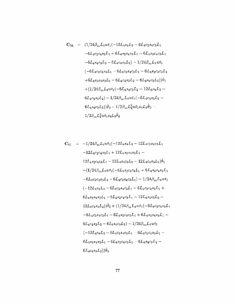
C 34 (1/24/3mL4 Wt(-12L4S 4 L 3 - 6L4c 2s4c 3 L1
-6L 4c 2c 4 s3 L1 + 6L4 s2 s 4s 3 L1 - 6L4 s2 c 4c3 L1
-6L 4s 4c 3L2 - 6L4 c4 s3L2 ) - 1/243mL4 wt1
(-6L4c 2c 4 s3 L -6L 4 c2s 4c3 L1 - 6L4s 2c4c 3 L1
+6L 4s 2S 4s3 L1 - 6L4c4 s 3L 2 - 6L4 s4c 3 L2 ))bl
+(1/24mL4Wt 1(-6L4S 4C 3 L 2 - 12L4s 4L 3 -
6L 4c4 s3 L2 ) - 1/24/3mL4Wtl(-6L4C4S3 L 2 -
6L 4s 4c3 L2 ))b 2 - 1/2/3mL4 tis 4 L3 3 -
1/20mL2Wts 4 L3 4
C4 1 -1/243mL 4 Wt(-12L4S 4 L 3 - 12L4 c2 84c 3 L1
-12L 4c 2c 4s 3 L1 + 12L4 s2 s4s3 L1 -
12L 4s 2c4c 3L1 - 12L4 s4 c3 L2 - 12L4c4 s3 L 2 )bl
+(1/24mL4Wt1(-6L 4s2 c 4c 3L1 + 6L4 s2 s4s 3 L1
-6L 4c 2c 4s 3L1 - 6L4 c2 s4 c3 L1 ) - 1/ 2 4 mL4Wt1
(-12L4s 4 L3 - 6L4c2 s4 c3 L1 - 6L4 c2c4 s3 L1 +
6L 4s 2s 4 s 3 L1 -6L 4 s2 c4c 3L1 -12L 4 s4 c3 L2 -
12L4 c4 s3L 2 ))b2 + (1/24/mL 4Wti(-6L 4C 2C 4S 3 L1
-6L 4c 2s 4c 3 L1 - 6L4 s 2c 4 C3 L1 + 6L4 s2s4s 3 L1 -
6L4c4 s3 L2 - 6L4s4 c3 L2 ) - 1/243mL 4Wt1
(-12L4s 4 L3 -6L 4 c2 s4c3 L1 - 6L4c2 c4 s3 L1 +
6L4sss 3L1 -6L 4 s2c4 c3L1 - 6L4 s4c 3L2 -
6L4 c4 s3L 2 ))0 3
77

C 42 (1/24/,3L4Wt1(-6L4S2C4C3L1 + 6L4 s2s4 s3 L1
-6L 4c 2c 4s3 L1 - 6L4 c2 s4c3L1 ) - 1/ 2 40mL4Wt1
(-12L4s 4 L 3 -6L 4 c2 s4c3 L1 - 6L4 c2 c4 s3 L1 +
6L 4 s2s4 s3 L1 -6L 4 s2 c4 c3 L1 -12L 4 s4 c3 L2 -
12L4 c4 s3L 2 ))Oi - 1/243mL4Wtl(-12L 4S 4C 3L 2
-12L 4s 4 L3 - 12L 4 c4 s3 L 2 )b2 + (1/243mL4Wti
(-6L4c 4s 3 L2 - 6L4 s4c3 L 2 ) - 1/24,mL4 Wtl
(-6L4s 4c 3 L2 - 12L 4s4 L 3 - 6L 4c4 s3 L2 ))b 3
C 43 = (1/240mL 4 Wtl(-6L4C2C4S3L1 - 6L4 c2 s4c3 L1
-6L 4s 2c 4c 3 L1 + 6L 4 s2 s4s 3 L1 - 6L4 c4 s 3L 2
-6L 4s 4c 3 L2 ) - 1/243mL4wt(-12L 4S 4 L3 -
6L 4c2 s4c3 L1 - 6L4c 2c4 s3 L1 + 6L4 s2 s4s 3 L1
-6L 4s 2c 4c 3L1 - 6L4s4 c3L2 - 6L4 c4 s3 L 2 ))b1
+(1/24mL4Wt1(-6L 4C 4 s3 L2 - 6L 4 s4c3L 2 )
-1/24,3mL 4Wt1(-6L 4S 4C 3L 2 - 12L4 s4 L3
-6L 4c4 s 3 L2 ))9 2 + 1/2I#mL4Wt s 4L3A 3
C44 = 0
78

Part II
Appendix B: Geometric and
Material Parameters for
Cube
79
Corner

The following parameters describe the corner cube geometry. The remaining material prop-
erties are equivalent to those defined in Appendix A.
Parameter Value Units
1 64 /Im
iC 71 pm
L 300 pmTable 3. Parameters for corner cube
The following represent the Jacobians, mass, and Coriolis matrices for the reduced open
chain system, respectively:
J1 =
J2 =
0
0
0.778L
-1
-1
0
0
0
0
0
0
0
-1/2s 2 L
1/2s2 L
1/2(-1 + c2 )L
-1
-c2
S2
0
0
0
0
0
0
0
0
1/2L
1
0
0
0
0
0
0
0
0
1/2(S3 - s 2c3 )L
1/2(83 - s 2c3 )L
-1/2(c2 + 83S2 + c3 )L
-8382 - c3
-C 2
-S3 + S2C3
80
J3 =
-1/2s 3L
-1/2s 3L
1/2Lc 3
C3
0
0
0
1/2L
0
1
S3 0

Ml= 0.33mL^4ti + 2,3m(1/24L2 t3 + 1/36L^4ti)
+2/3s2L^4mti + 1/4(-1 + C2 ) 2 L^40mti +
1/12/3mL 2 ti(L2 + tl) + 1/12C2/3mL 2ti(L 2 + t2)
+1/12mL 2 t,(12L 2 - 8L 2S3 S2c 3 - 4L 2 c2c2 +
6L 2c2 s3S 2 + 6L2c2 c3 + + t1c c + 2s3s2c3ti)
M12 = 1/4(-1 + C2 )L^40mti - 1/12/mL 2ti(L2 + t2)
-1/12/3mL 2ti(8L 2 - 4L 2c2 - 4L 2s 3s 2c 3 +
3L2c2 c3 + s3 s 2c3 t1 + 1)
M13 -1/12mL 2ti(4L2 C2 + 3s 3 s 2 L2 + 3L2 c 3 + c2 t )
M21 = 1/4(-1 + c)L^4/mti - 1/123mL 2ti(L 2 + t2)
-1/l2OmL 2 t,(8L2 - 4L 2 c2 - 4L 2 s3 s 2c 3 +
3L 2 cC + s3s2c3t + cat2)
M22 =1/4/mL^4ti + 1/123mL 2 t (L 2 + t2) +
1/12mL 2 ti(8L2 - 4L2 c2 + cit2)
M23 = 1/4L^4C30mti
81

M31 = -1/120mL 2ti(4L2 C 2 + 3s3 s 2 L2 + 3L2 c 3 + c2t )
M32 = 1/4L^4C 3Imti
M33 = 1/33mL^4ti + 1/120mL2t
Cii = (2/3s2 L^43mtiC2 - 1/4(-1 + C2 )L^4/3mtiS 2
-1/12c 2QmL2ti(L2 + t2)S2 + 1/24/mL 2 t,
(-8L 2s 3c 2c 3 + 8L 2c2c 2 8 2 - 6L 2 S2s 3 + 6L 2c2s 3
-6L 2s2 c 3 - 2t c2c s2 + 2s3c2c3t1))b2 +
1/240mL 2 t1(-8L 2C2S 2 + 8L2 s2 s 2 + 8L 2c3c2s 3
+6L 2c 2c3s 2 - 6L 2c2 S3 - 2t2c2c3 s3 +
2c2s2 t2 - 2sis2 t2)O3
C 12 = (2/3S 2 L^40mtiC 2 - 1/4(-1 + c2)L^43mtiS 2
-1/12C 2ImL2 ti(L 2 + t2)S2 + 1/24/mL2 t,
(-8L 2S 3c 2c 3 + 8L 2c2c 2S 2 - 6L 2 S2s 3 + 6L 2c2s 3
-6L 2s 2c 3 - 2t2c2c2s2 + 2s3 c2c 3t2))Oi +
(-1/4 2L^4mti - 1/12#mL 2 ti(-4L2S 3C2 C3 -
3L 2s 2 c 3 + s3 c2 ctI)) 2 + (-1/240mL2 ti(8LC3S 3
-4L 2c2s 2 + 4L 2s2s 2 - 3L 2 c2 s3 + Cs2 t -
ss 2 tl - 2c3t s3) - 1/243mL 2 t(-4L2 S2 +
3L 2c2 s3 - S2 f))3
82

C 13 = 1/243mL2t,(-8L2Cjs2 + 8L 2s2s 2 + 8L 2 c3c2s 3
+6L 2c 2c 3s 2 - 6L2 c2s 3 - 2t2c2c3s3 + 2c2s2t2
-2s s2 t)bl + (-1/243mL2 t,(8L2C 3S 3 -
4L 2c2s 2 + 4L 2s2 s 2 - 3L2 C2S3 + c2 st2 - s2 st 2
-2c 3t s 3 ) - 1/24mL 2 t(-4L2 s2 + 3L2c2 s3
-s2ti))b2 - 1/12/mL 2ti(3LS2C 3 - 3L2S 3 )b 3
C 21 = (-2/3 2L^4mtiC 2 + 1/4(-1 + C2 )L^43mtiS 2
+1/12C 2/mL 2 ti(L2 + t2)s2 - 1/24/3mL 2t,
(-8L 2s 3c 2c 3 + 8L2 c2c2 s 2 - 6L2 s s3 +
6L 2c2s 3 - 6L2 s 2c3 - 2tic2 csC 2 + 2s 3c2 c3t!))2 i
+(-1/240mL 2t1(8L2C3S 3 - 4L 2c2s 2 + 4L 2 s2s 2
-3L 2c2 s 3 + cI2t- s 2tI - 2c3t s 3 ) +
1/240mL 2 t1 (-4L2 S 2 + 3L2 c2 S 3 - 82)A
C2 2 = 1/24#mL2 ti(8LC3S 3 - 2c3t s3)O3
C 23 = (-1/240mL2t(8L 2C3 83 - 4L 2c2s 2
+4L 2s2s 2 - 3L2 c2s 3 + cs s2t2 - s s2 t2
-2c 3tls 3 ) + 1/24#mL 2 ti(-4L2 S2 +
3L 2c2 S 3 - S2 t))b1 + 1/24/mL 2 t,
(8L2 c3s3 - 2c3 t s3)b2 - 1/4L^4S 3 0mtO 3
83

C3 1 -1/24/mL 2t,(-8L2C2S2 + 8L 2 s2s 2 +
8L2 c3cs3 + 6L 2c2c 3s 2 - 6L 2c2 83
-2t2c2c 3s3 + 2c2s2 t2 - 2s s2 t2)Oi +
(-1/240mL2t,(-4L2S 2 + 3L 2c2 s3 -
s2 t2) + 1/243mL2t(8L2C 3S 3 - 4L2cjs2
+4L 2ss2 - 3L 2 c2s 3 + c2s2t 2- s2s2 t2
-2c 3tIs 3 )) 2
C 32 = (-1/24mL2t,(-4LS2 +3L2 C 2S 3
-s 2 t2) + 1/240mL2t,(8L2C 3S 3 - 4L2cjs2
+4L 2ss2 - 3L 2c2 s3 + c2s2t 2- s2s2 t2
-2c3tIs3))i - 1/243mL 2 t (8L2 c3 s 3
-2c 3t s 3 )b2
C 33 = 0
84

Bibliography
[1] S.M. Jurga, "3D micro and nanomanufacturing via folding of 2D membranes," M.S. Thesis.
In Dept. of Mechanical Engineering. Cambridge, MA: Massachusetts Institute of Technol-
ogy, 2003, pp. 16-42, 77-96.
[2] J.T. Hastings, F. Zhang, and H.I. Smith, "Nanometer-level stitching in raster-scanning
electron-beam lithography using spatial-phase locking," Journal of Vacuum Science &
Technology B, vol. 21, pp. 2650-2656, 2003.
[3] M. Qi, E. Lidorikis, P. T. Rakich, S. G. Johnson, J. D. Joannopoulos, E. P. Ippen and
H. I. Smith, "A three-dimensional optical photonic crystal with designed point defects,"
Nature, vol. 429, pp. 538-542, 2004.
[4] M.C. Purdy. (2005, September 2.2). Atlas of the folds of
the cerebral cortex. Medical News Today [Online]. Available:
http://www.medicalnewstoday.com/medicalnews.php?newsid=30973.
[5] C. Ho and M. Madrid (2005). Looking for a blood substi-
tute. Pittsburgh Supercomputing Center Website [Online]. Available:
http://www.psc.edu/science/Ho/Ho.html#hemoglobin.
[6] N. Amato and G. Song, "Using Motion Planning to Study Protein Folding Pathways,"
Journal of Computational Biology, vol. 9, no. 2, pp. 149-168, April 2002.
[7] H.J. In, S. Kumar, Y. Shao-Horn, and G. Barbastathis, "Origami Fabrication of
Nanostructured 3D Devices: Electrochemical Capacitor with Carbon Electrodes," Applied
Physics Letters, to appear.
85

[8] J.B. Pendry, "A Chiral Route to Negative Refraction," Science, vol. 306, no. 5700, pp.
1353-1355, 19 November 2004.
[9] M.C.K. Wiltshire, J.V. Hajnal, J.B. Pendry, D.J. Edwards, and C.J. Stevens, "Meta-
material endoscope for magnetic field transfer: Near field imaging with magnetic wires,"
Optics Express, vol. 11, no. 7, April 2003, pp. 709-715.
[10] J. Cybulski, "Modeling and Fabrication of Self-Assembling Micron-Scale Rollup Struc-
tures," M.S. Thesis. In Dept. of Mechanical Engineering. Cambridge, MA: Massachusetts
Institute of Technology, 2004.
[11] W. Arora, A. Nichol, H.I. Smith, and G. Barbastathis, "Membrane folding to achieve
three-dimensional nanostructures: nanopatterned silicon nitride folded with stressed
chromium hinges," Applied Physics Letters, to appear.
[12] I. Streinu, "Pseudotriangulations, rigidity, and motion planning," Discrete and Com-
putational Geometry, vol. 34, no. 4, pp. 587-635, Dec. 2005.
[13] R. Connelly, E.D. Demaine, and G. Rote, "Straightening polygonal arcs and convexi-
fying polygonal cycles." In Proceedings of the 41st Annual Symposium on Foundations of
Computer Science (FOCS 2000), Redondo Beach, California, November 12-14, 2000, pp.
432-442.
[14] R. Connelly, E.D. Demaine, and G. Rote, "Straightening polygonal arcs and con-
vexifying polygonal cycles." Discrete and Comp. Geometry, 30 (2): 205-239, September
2003.
[15] J.H. Cantarella, E.D. Demaine, H.N. Iben, and J.F. O'Brien, "An energy-driven ap-
proach to linkage unfolding." In Proceedings of the 20th Annual A CM Symposium on Com-
putational Geometry, Brooklyn, NY, June 2004.
[16] I. Streinu, "A combinatorial approach to planar non-colliding robot arm motion plan-
ning." In Proc. 41st Annual IEEE Sympos. Found. Comput. Sci. IEEE, November 2000.
pp. 443-453.
[17] E.D. Demaine, "Folding and Unfolding." Ph.D. Thesis. In Dept. of Computer Science.
University of Waterloo, Canada, 2001.
86

[18] E.D. Demaine and J. O'Rourke. Geometric Folding Algorithms: Linkages, Origami,
and Polyhedra. Book in preparation, Cambridge University Press.
[19] E.D. Demaine, M.L. Demaine, and J.S.B. Mitchell, "Folding flat silhouettes and wrap-
ping polyhedral packages: new results in computational origami," Comput. Geom. Theory
Appl., 16 (1):3-21, 2000.
[20] I. Streinu and W. Whiteley, "Single-vertex origami and 3-dimensional expansive mo-
tions." In Proc. Japan Conf. Discrete and Comp. Geometry, Tokai University, Tokyo,
Japan, Oct. 8-11, 2004.
[21] s.m. belcastro and T. Hull, " Modeling the folding of paper into three dimensions using
affine transformations," Linear Algebra and its Applications, vol. 348, pp. 273-282, 2002.
[22] T. Buchner, "Kinematics of 3D Folding Structures for Nanostructured Origami,"
Diploma Thesis, Laboratory for Machine Tools and Production Engineering, RWTH
Aachen University (2004), URL: web.mit.edu/optics/www/publications/.
[23] R.M Murray, Z. Li, and S.S. Sastry, A Mathematical Introduction to Robotic Manipu-
lation. Boca Raton, FL: CRC Press, 1994, Ch. 2-5.
[24] R.P. Paul, Robot Manipulators: Mathematics, Programming, and Control. Cambridge,
MA: Massachusetts Institute of Technology, 1981.
[25] H. Asada and J.J. Slotine, Robot analysis and control, New York: Wiley, 1986.
[26] J. Wittenburg, Dynamics of Systems of Rigid Bodies. Stuttgart: B.G. Teubner, 1977.
[27] J.Y.S. Luh and Y. Zheng, "Computation of Input Generalized Forces for Robots with
Closed Kinematic Chain Mechanisms," IEEE J. Robotics Automat., vol. RA-1, no. 2, pp.
95-103, June 1985.
[28] J.J. Murray and G.H. Lovell, "Dynamic modeling of closed-chain manipulators and
implications for trajectory control," IEEE Transactions on Robotics and Automation, vol.
3, no. 4, pp. 522-528, August 1989.
[29] Y. Nakamura and M. Ghodoussi, "A computational scheme of closed link robot dy-
namics derived by D'Alembert Principle," In Proc. 1988 IEEE Int. Conf. on Robotics and
Automation, Philadelphia, PA, Apr. 24-29, 1988, pp. 1354-1360.
87

[30] H. Baruh, Analytical Dynamics. McGraw-Hill, 1999, p. 253-302.
[31] J.R. Barber, Intermediate Mechanics of Materials. New York: McGraw-hill, 2001, p.
107.
[32] Nielson, G.N., Seneviratne, D., Lopez-Royo, F., Rakich, P.T., Avrahami, Y., Watts,
M.R., Haus, H.A., Tuller, H.L., and Barbastathis, G. "Integrated wavelength-selective
optical MEMS switching using ring resonator filters," IEEE Photonics Technology Letters,
vol. 17, no. 6, pp. 1190-1192, June 2005.
[33] N. Razmara, D. Kohli, and A.K. Dhingra, "On the degrees of freedom of motion of
planar-spatial mechanisms," In Proc. ASME 2000 Design Engineering Technical Confer-
ences and Computer and Information in Engineering Conference, Baltimore, MD, Sept.
16-17, 2000.
88