virtual design from nature: kinematic modeling of the

2010 SIMULIA Customer Conference 1

Virtual design from nature: Kinematic modeling of the seahorse tail

Sofie Van Cauter1, Dominique Adriaens2, Srikanth Kannan3, Srikanth Srigiriraju3, Tomas Praet1, Bert Masschaele4, Matthieu De Beule1 and Benedict Verhegghe1

1 Institute Biomedical Technology (IBiTech), Ghent University, Ghent, Belgium 2 Evolutionary Morphology of Vertebrates (Dept. of Biology), Ghent University, Ghent, Belgium

3 SIMULIA HQ, Providence, RI, USA 4 Centre for X-ray Tomography (UGCT), Ghent University, Ghent, Belgium

Abstract: Seahorses (belonging to the genus Hippocampus) and pipehorses are unique among fishes in being armed with robust body plates instead of scales, and in being able to bend their tail ventrally for use as a prehensile appendage. They lack a powerful caudal fin, making them very slow swimmers, which can hardly escape predatory fish. However, they have survived millions of years of natural selection, yielding a very well camouflaged fish with a highly specialized caudal skeleton. This skeleton consists of a central axis of articulating vertebrae, surrounded by jointed bony rings. The stiff bony plates form an armor, which likely makes the fish strongly resistant to bites and unappetizing for predators. However, the adaptive nature of the articulated segments may also be in relation to the formation of the flexible, prehensile tail, which can roll up ventrally over more than 360 degrees and enables the seahorse to grasp and hold onto a support. The tail bending mechanism of seahorses has been studied superficially in literature, but details of its functioning and constructional morphology are lacking. To gain a profound insight into the kinematics and mechanical interactions of the skeletal elements of the tail, the musculoskeletal system is modeled, combining pyFormex with Abaqus, using various features such as beam connectors (bony plates and vertebrae), cartesian, cardan and slot connectors (joints) and axial connectors (muscles). Such modeling may allow the design of nature-inspired structures, providing innovative solutions in engineering where high stiffness combined with high flexibility is needed.

Keywords: Seahorse, Prehensile Tail, Musculoskeletal Model, Nature-Inspired Design

1. Introduction

Evolution of living organisms by means of natural selection, and involving adaptations, can be considered as the biological analogue to a prototype development and testing in engineering, where a functional system is to be obtained. The advantage of the biological version is that the testing phase generally spans millions of years and generations, where every reduction in functionality results in its disappearance or its improvement (Futuyma, 1998). Living systems are the result of such a rigorous selective process where adaptations have given rise to the most spectacular functioning complexities. Especially musculoskeletal systems of articulating elements

2 2010 SIMULIA Customer Conference

are subjected to the same mechanical constraints and rely on similar material properties as those encountered in engineering (Wainwright, 1976). One such a system is the tail of pipehorses and seahorses (Figure 1). Belonging to the order Syngnathiformes, these fishes have a body covered with bony plates, unlike most other bony fishes, which only have internal bones for support and scales for protection. Moreover, pipehorses and seahorses have a tail system that is unique to all other bony fishes in that it became modified into a prehensile organ used to grasp onto objects on the seafloor. The tail system from which this seahorse grasping structure has originated, is one used for swimming, so bearing a terminal caudal fin and is considered to be similar to the one found in their closest allies the pipefishes (Figure 2). It has been hypothesized that prior to having a tilted head (another unique feature), these fishes developed the prehensile tail somewhere at the beginning of the Oligocene, when the seahorses obtained their vertical posture during the mid-Oligocene, at the moment large seagrass beds were formed along the coastal Indo-West-Pacific (Teske, 2009). Having this vertical posture and a prehensile tail allowed the seahorses to grasp onto the seagrass, which improved their camouflage.

Figure 1: Skeleton of an adult seahorse (belonging to the species Hippocampus reidi) obtained from a micro-CT reconstruction, showing the chain of skeletal elements surrounding and protecting the body. Caudally, the curved prehensile tail is shown.

In pipefishes, the caudal musculature lies along the vertebral column, being enclosed within a chain of articulating dermal bony plates (Figure 2). This articulated system, having joints between as well as within the chain segments, provides both for strength (for protection against predators and for dealing with mechanical stress during swimming) and flexibility (for allowing undulatory movements during swimming). However, already in pipefishes, the caudal system is not the only


propelling structure, as the dorsal fin is also involved. This may have facilitated an evolutionary shift from a swimming tail towards a grasping tail, as seahorses still largely rely on their dorsal fin as an engine for propulsion (Consi, 2001). A decoupling of the tail system from the typical lateral undulatory movements may well have been a crucial step towards the origin of a prehensile system where bending in a dorsoventral direction is important. Observations on the use of this tail in seahorses have indeed shown that bending mainly occurs in a ventral direction during grasping, although lateral bending is still possible (Hale, 1996; Peters, 1951). It thus seems evident that this evolutionary shift in functionality only became possible after several structural modifications had occurred. It can thus be hypothesized that this may have involved: (1) change in shape of the dermal plates, (2) change in both the morphology and physical properties of the joints between the plates (both within and between body segments), (3) change in the morphology and physical properties of the connections between the vertebrae and the dermal plates, and (4) change in the way the caudal muscles insert onto the dermal plates and control for grasping movements.

Figure 2: Habitus of a pipefish (Microphis brachyurus) showing the chain of skeletal plates covering the whole body, including the tail.

In order to better understand how these skeletal elements, i.e. vertebrae and dermal plates, interact with each other during grasping, the main components of the musculoskeletal tail system that are involved in the bending mechanism, were modeled using Abaqus. The model comprises the individual skeletal elements of several segments of the tail system, the joints that connect these skeletal elements and the muscles that allow the tail to bend. Applying a deformation to the muscles will cause the tail to bend by joint movement (rotation and/or translation). Vice versa, moving the endpoint of the tail to a certain position will result in joint movement and muscle deformation. Such simulations will allow an understanding of how the movements of the individual elements are constrained during grasping.

2. Material and methods

2.1 Morphology

For this study, the species Hippocampus reidi was used. A specimen was obtained through the pet trade, anaesthetized using an overdose of MS222 (Sigma), fixed in a 10% formalin solution and stored in ethanol 70%.

A micro-CT scan, with a spatial resolution of about 21 µm, was made in the Centre for X-ray Tomography (http://www.ugct.ugent.be) of the Ghent University. The sample was fixed in a plastic cylindrical tube and placed on an accurate rotation stage. During the CT scan hundreds to more than a 1000 radiographic X-ray projections are taken from different angles in an angular interval of 360°. On average, the total scanning time is about 1 to 1.5 hours. During the entire scan period, the sample and the sample holder are not allowed to move (except for the CT rotation),


which is often difficult with samples that are taken out of the formaldehyde. For the measurements, we used a Hamamatsu L9181 microfocus tube, an air-bearing rotation stage (Aerotech, Ltd) and an amorphous silicon flat panel detector (Paxscan 2025V by Varian). All components are placed on motorized stages, which allow to vary the scanning geometry or to select a different X-ray tube or X-ray detector. For the data reconstruction, the Octopus package (http://www.inCT.be) was used. Octopus allows to process the raw data into hundreds of cross-sectional slices through the sample. Each pixel in a slice contains information about the local electron density in the scanned volume. This density is a function of the mass density and the material composition. High density or elements with a high atomic number lead to high CT values. CT is therefore an ideal tool to obtain information about the bone structure since, in general, bone contains a large amount of mineralized calcium.

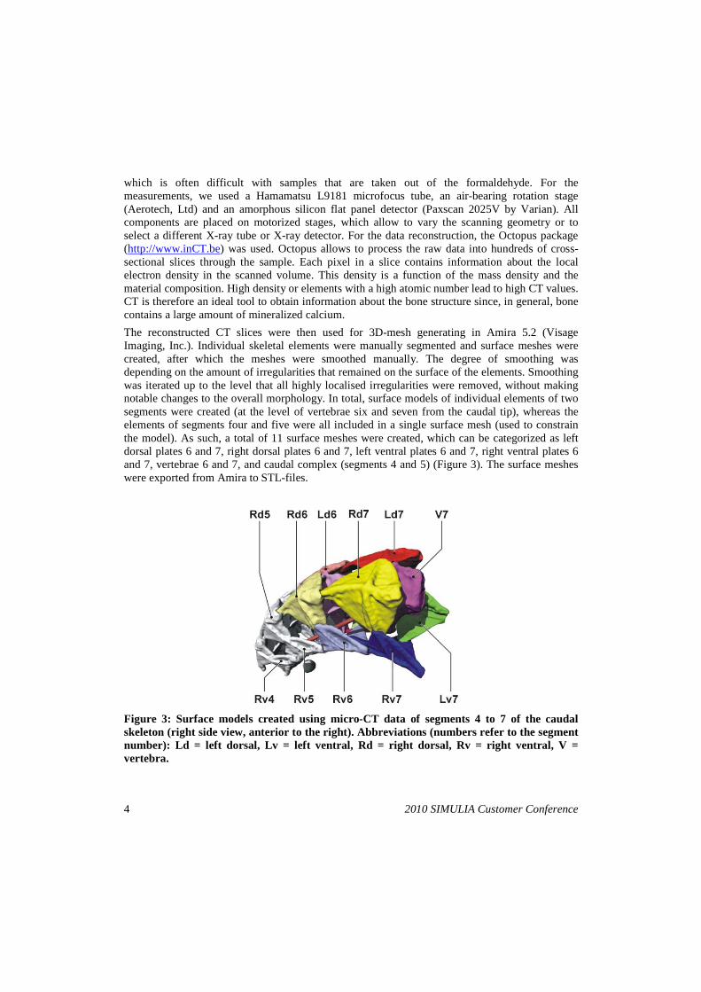
The reconstructed CT slices were then used for 3D-mesh generating in Amira 5.2 (Visage Imaging, Inc.). Individual skeletal elements were manually segmented and surface meshes were created, after which the meshes were smoothed manually. The degree of smoothing was depending on the amount of irregularities that remained on the surface of the elements. Smoothing was iterated up to the level that all highly localised irregularities were removed, without making notable changes to the overall morphology. In total, surface models of individual elements of two segments were created (at the level of vertebrae six and seven from the caudal tip), whereas the elements of segments four and five were all included in a single surface mesh (used to constrain the model). As such, a total of 11 surface meshes were created, which can be categorized as left dorsal plates 6 and 7, right dorsal plates 6 and 7, left ventral plates 6 and 7, right ventral plates 6 and 7, vertebrae 6 and 7, and caudal complex (segments 4 and 5) (Figure 3). The surface meshes were exported from Amira to STL-files.

Figure 3: Surface models created using micro-CT data of segments 4 to 7 of the caudal skeleton (right side view, anterior to the right). Abbreviations (numbers refer to the segment number): Ld = left dorsal, Lv = left ventral, Rd = right dorsal, Rv = right ventral, V = vertebra.


The morphology of the skeletal elements and joints was described by studying these surface meshes. Detailed information on the attachment locations of those muscles involved in tail bending, was obtained from literature (Hale, 1996). Two muscles that are assumed to be crucial for ventral bending were used for this model: the myomere muscles and median ventral muscles (for a description, see results).

2.2 Kinematic analysis

The musculoskeletal system was then modeled in Abaqus/CAE. The skeletal elements (vertebrae and dermal plates) were imported by reading the STL-files and modeled with beam connections from the center of mass to several attachment points as shown in Figure 4. The mass of the skeletal elements was determined by calculating the volume and multiplying this with a density of 1800 kg/m3 (Biltz, 1969) and was distributed over the connector nodes by creating mass elements. Furthermore, mass properties were determined using Abaqus/CAE and inertia elements were used to assign rotary inertia to the nodes. The joints and muscles between the skeletal elements were added by creating connectors. The sliding joints along the caudal processes of all four plates in one segment that fit into the medial grooves of all corresponding plates of the segment posterior to it and the overlapping joints between all plates within one segment have been modeled using SLOT+CARDAN connectors in Abaqus (see Results for a description of these skeletal elements and their connections). SLOT provides a slot connection to make the position of the second node remain on a line defined by the orientation of the first node and CARDAN provides a rotational connection between two nodes. The fixed ball-and-socket joints between the lateral processes of the vertebrae and the dorsal plates and the joints between the vertebrae (see Figure 6) were modeled using CARTESIAN+CARDAN connectors. CARTESIAN provides a connection between two nodes that allows independent behavior in three local Cartesian directions. Myomere muscles and median ventral muscles were modeled using AXIAL connectors, which provide a connection between two nodes that acts along the line connecting the nodes. The complete seahorse model in Abaqus/CAE is shown in Figure 5.

Figure 4: Beam connection representation of dermal plate.


Figure 5: Complete seahorse model in Abaqus/CAE.

2.3 Automated pre-processing

The skeletal elements clearly vary in size along the tail, but they seem to have a highly uniform shape (see Figure 1). Therefore, dedicated pre-processing of this musculoskeletal model, including the (semi)-automatic creation of joints and muscles, seems both advisable and feasible. The approximate joint locations and muscle attachments can be computed by using relative lengths and shape characteristics such as principal axes. In addition, the joint and muscle connectors can be automatically created based on these locations and by using predefined connector types and properties.

A first step towards automated pre-processing was performed in this study. After studying the locations of the muscle insertions, a standardized method was developed to automatically locate the attachment points on the surface meshes and was tested on the two tail segments. The algorithm was implemented in pyFormex (http://pyformex.berlios.de), which is an open-source software program intended for generating, manipulating and operating on large geometrical models of 3D structures.

3. Results

3.1 Morphology

A single segment in the chain of skeletal elements in a seahorse tail comprises a central vertebral element, surrounded by four dermal plates (Figure 6). The vertebra itself bears four processes, i.e. a small dorsal one (i.e. the neural spine), a large ventral one (i.e. the haemal spine) and two lateral ones (i.e. the transversal processes). The dermal plates themselves each comprise two planes that are positioned perpendicular to each other. A close contact between the vertebra and these plates is only established between the dorsal and transversal vertebral processes and the two dorsal dermal plates. The dorsal process is connected


to the anterior rim of the dorsal plates, at the level where they form an overlapping joint. The lateral processes seem to form a more solid contact with the medial face of the vertical part of the dorsal plates, where some kind of ball-and-socket joint is present. As such, the whole chain of skeletal elements seems to be suspended from the vertebral column mainly at the level of the dorsal part, with the ventral part being suspended from the dorsal plates. This is established by overlapping joints between the dorsal and ventral plates, with the ventral ones lying superficially against the dorsal ones. The left and right ventral plates are connected by a similar joint. Whether left is overlapping right or vice versa seems to be variable along the caudal system. What all overlapping joints do have in common is that the degrees of freedom of this connection seem to be constrained due to the presence of a bony ridge on the outer surface of the plates, and a similarly directed furrow on the inner surface. This suggests that movement within a single segment is largely constrained to translation, i.e. mediolateral for the joints between left and right side plates, and dorsoventral for the joints between dorsal and ventral plates. A similar, but more elaborate ridge-in-furrow joint is present between the plates of the consecutive segments. A distinct caudal process is present on each dermal plate, at the level where the two perpendicular planes of these plates meet. This extended process then fits into a medial furrow on the dermal plate of the segment posterior to it. Such a connection is present on both sides, both dorsally and ventrally.

Figure 6: Skeletal elements of segment 7, showing the details of the connections and processes of the plates and vertebra (left: oblique left anterior view; right: oblique left posterior view). Abbreviations: DC = dorsal connection between dermal plates and vertebra; LC = lateral connection between dermal plates and vertebra; Ld7 = left dorsal, Lv7 = left ventral, Rd7 = right dorsal, Rv7 = right ventral, V7 = vertebra 7, Rv7-gr = medial groove of the right ventral plate; Rv7-pc = caudal process on the right ventral plate (similar terminology for other plates); V7-pt = transverse process of the vertebral body , V7-pv = ventral process of the vertebral body.


Several muscle bundles surrounding the vertebral elements are confined within the volume enclosed by the dermal plates. These muscles are derived from the epaxial musculature (so-called myomeres) and from the muscles that normally interact with the anal fin in other bony fishes (the median ventral muscles) (Figure 7). Only those muscles that seem to be involved in a ventral curving of the caudal system are illustrated here as bars between the skeletal elements that they insert onto. The myomeres are biarticulate muscles, spanning three vertebrae. They originate on the caudal margin of the lateral process of a vertebra, run below the lateral process of the vertebra posterior to it, and then insert onto the medial face of the ventral plates of the next segment posterior to that. A bilateral contraction can be expected to induce a ventral curving of the tail, whereas a unilateral contraction may generate a left-right bending. The medial ventral muscles are uni-articulate, running from the posterior face of the ventral process of a vertebra to the anterior face of the ventral process of the vertebra lying posterior to it. Contraction will induce a ventral bending of the tail at the level of the vertebrae.

Figure 7: Skeletal elements of segments 4 to 7, with dermal plates of segment 6 and 7 removed, showing the position and attachment of the two main muscles for ventral bending (right side view, anterior to the right). Abbreviations: Mm-m = myomere muscle, Mv-m = medial ventral muscle, V = vertebra, V-pt = transverse process of the vertebral body, V-pv = ventral process of the vertebral body.

3.2 Kinematic analysis

In order to ensure that the model is kinematically determinate and avoid numerical instability, skeletal elements must be kinematically constrained properly and appropriate mass properties should be applied to them. Preliminary tests were run by applying a boundary condition to segments 4 and 5 and connector forces and motion were measured. As seen from Figure 8 (right), the connector forces are very low and thus ensure that the model is constrained properly. Connector motion of the median ventral muscles was measured from the first boundary condition analysis as seen in Figure 8 (left). Because the tail was curved during micro-CT scanning, it was constrained to stretch during the first analysis. The applied boundary condition results in extension

2010 SIMULIA Customer Conference

for the median ventral muscle between vertebra 6 andmuscle (blue) and in contraction for the left myomere muscle (red), while the length of the median ventral muscle between vertebra 7 and 6 (green) barely changes. measured connector motion was applied to the median ventral muscles and segmenfixed. Figure 9 shows the displacement of the entire seahorse model with respect to time. extension of the median ventral muscle between vertebra 6 and 5 causes the tail to stretch at thejoint between these vertebrae. However, there is 7 and 6, because of the unchanged length of the median ventral muscle between these vertebrae. Segments 6 and 7 enlargeventral plates of these segmentsthe segments 6 and 5. The trajectory of the center of mass of the skeletal elements of segment 7 were measured and plotted as seen in connectors is plotted in Figureand left ventral plates of segment 7

Figure 8: (Left): Connector motion output of musclesbetween vertebra 7 and 6, yellow: median ventral muscle between vertebra 6 and 5, red: left myomere muscle, blue: right myomere muscle)elements.

Figure 9: Undeformed and d


ral muscle between vertebra 6 and 5 (yellow) and for the right myomere and in contraction for the left myomere muscle (red), while the length of the median

ventral muscle between vertebra 7 and 6 (green) barely changes. In the second analysis, the measured connector motion was applied to the median ventral muscles and segmen

shows the displacement of the entire seahorse model with respect to time. extension of the median ventral muscle between vertebra 6 and 5 causes the tail to stretch at thejoint between these vertebrae. However, there is barely no stretching at the joint between vertebra 7 and 6, because of the unchanged length of the median ventral muscle between these vertebrae. Segments 6 and 7 enlarge mainly by sliding at the overlapping joints between the

these segments and at the overlapping joints along the caudal processesThe trajectory of the center of mass of the skeletal elements of segment 7

were measured and plotted as seen in Figure 10 (left). The motion of one of the igure 10 (right), which shows the sliding action between

of segment 7 along the local x-axis.

: (Left): Connector motion output of muscles (green: median ventral muscle between vertebra 7 and 6, yellow: median ventral muscle between vertebra 6 and 5, red: left myomere muscle, blue: right myomere muscle); (Right): Connector forces in connector

Undeformed and deformed shape of seahorse model in Abaqus/Viewer

9

5 (yellow) and for the right myomere and in contraction for the left myomere muscle (red), while the length of the median

In the second analysis, the measured connector motion was applied to the median ventral muscles and segment 4 and 5 were

shows the displacement of the entire seahorse model with respect to time. The extension of the median ventral muscle between vertebra 6 and 5 causes the tail to stretch at the

barely no stretching at the joint between vertebra 7 and 6, because of the unchanged length of the median ventral muscle between these vertebrae.

oints between the dorsal and along the caudal processes between

The trajectory of the center of mass of the skeletal elements of segment 7 SLOT+CARDAN

which shows the sliding action between the left dorsal

(green: median ventral muscle between vertebra 7 and 6, yellow: median ventral muscle between vertebra 6 and 5, red: left

(Right): Connector forces in connector

eahorse model in Abaqus/Viewer.


Figure 10: (Left): Node trajectories of the center of mass of the plates and vertebrae of segment 7; (Right): Initial and final configuration of SLOT+CARDAN connector between left dorsal and left ventral plate of segment 7 .

3.3 Automated pre-processing

To automatically locate the muscle attachment points, a three-step procedure was implemented in pyFormex (serving as a dedicated pre-processor for Abaqus): (1) orient the skeletal elements in a standardized way; (2) extract the anatomical part, to which the muscle is attached and (3) determine the attachment points on the anatomical part.

The median ventral muscles originate on the posterior face of the ventral process of a vertebra and insert onto the anterior face of the ventral process of the vertebra lying posterior to it. Therefore, the surface model of the vertebra was first oriented using the principal axes of inertia (PAOI). In order of decreasing principal moments of inertia (PMOI), these axes correspond approximately to the left-right, dorsoventral and anteroposterior lines. Next, the ventral process was extracted as follows. An initial ventral process is calculated as the 30% most ventral part of the vertebra and the PAOI of this most ventral part are calculated. The axis with the smallest PMOI (v3) represents the main direction of the ventral process and is oriented posteroventrally (see Figure 11). Because the PAOI depend on the axis along which the ventral process is calculated, this procedure is repeated (calculate the ventral process as the 30% most extreme part of the vertebra along v3; calculate v3 as the third PAOI of the ventral process) until the angle between two consecutive v3 directions converges. If the angle converges to zero, a single solution is found. If the angle converges to a value greater than zero, the process iterates between two directions v3. In this case, a final iteration is performed, using the mean of these directions. Finally, the attachment points of the median ventral muscles were computed by the method that is illustrated in Figure 11:

• ctr = center of gravity of the ventral process

• v1, v2, v3 = PAOI of the ventral process (in order of decreasing PMOI)

• Anterior attachment point of the median ventral muscle (Mv-m-Apv)

o Shift ctr to point at 85% of length along v3


o Take parallel line to v2 through this point

o Compute most anterior intersection point of this line with the ventral process

o Take closest node as Mv-m-Apv

• Posterior attachment point of the median ventral muscle (Mv-m-Ppv)

o Shift ctr to point at 50% of length along v2


o Compute most ventral intersection point of this line with the ventral process

o Take closest node as Mv-m-Ppv

The percentages were chosen to approximate the muscle attachment locations found in literature. However, this method allows to easily adjust the points by specifying different percentages or by using varying percentages based on the location of the segment in the tail.

Figure 11: Attachment points (red dots) of the median ventral muscles on the ventral process of the vertebral body (left: oblique right ventral view; right: projection). Abbreviations: ctr = center of gravity, v1,v2,v3 = principal axes of inertia, Mv-m = medial ventral muscle, Apv = anterior attachment point on the ventral process, Ppv = posterior attachment point on the ventral process.

The myomere muscles originate on the posterior face of the lateral processes of the vertebra and insert onto the medial face of the ventral dermal plates. The left and right lateral processes are calculated as the 25% most left and right parts of the oriented vertebra. A global lateral process is defined as the combination of the left and right processes. A converged solution is found by using a similar iterative procedure as for the ventral process (v3 is the third PAOI of the lateral process and the lateral process is calculated as the 25% most extreme parts of the vertebra along v3). The attachment points of the myomere muscles are shown in Figure 12:

• ctr = center of gravity of the lateral process

• v1, v2, v3 = PAOI of the lateral process (in order of decreasing PMOI)

12

• Left attachment point

o Shift ctr to point at 80%


o Compute

o Take closest node as

• Right attachment pointpoint at 20% of length along v3

Figure 12: Attachment points (red dots) of the myomere muscles on the of the vertebral body (left: oblique posterior dorsal view; right: projection).ctr = center of gravity, v1,v2,v3 = principal axes of inertia, left attachment point on thetransverse processes.

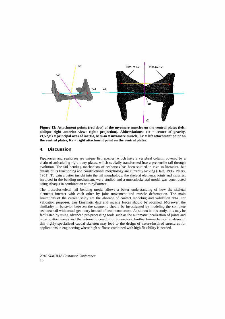
The left and right ventral plates were mergedattachment points of the myomere muscles (Figure 13):

• ctr = center of gravity of the ventral plates

• v1, v2, v3 = PAOI of the ventral plates (in order of decreasing

• Left attachment point

o Shift ctr to point at 50% of length along v1 and 25% of length along v2


o Compute

o Take closest node as

• Right attachment intersection point with the right ventral plate


attachment point of the myomere muscle (Mm-m-Lpt)

to point at 80% of length along v3

Take parallel line to v2 through this point

Compute most posterior intersection point of this line with the lateral process

Take closest node as Mm-m-Lpt

Right attachment point of the myomere muscle (Mm-m-Rpt): analogous, starting from point at 20% of length along v3

Attachment points (red dots) of the myomere muscles on the transverse(left: oblique posterior dorsal view; right: projection).

ctr = center of gravity, v1,v2,v3 = principal axes of inertia, Mm-m = myomereattachment point on the transverse processes, Rpt = right attachment point on the

The left and right ventral plates were merged into one object and the PAOI were computed.attachment points of the myomere muscles on the ventral plates were then extracted

ctr = center of gravity of the ventral plates

v1, v2, v3 = PAOI of the ventral plates (in order of decreasing PMOI)

Left attachment point of the myomere muscle (Mm-m-Lv)

to point at 50% of length along v1 and 25% of length along v2

Take parallel line to v3 through this point

Compute most medial intersection point of this line with the left ventral plate

Take closest node as Mm-m-Lv

point of the myomere muscle (Mm-m-Rv): analogous, most intersection point with the right ventral plate


with the lateral process

: analogous, starting from

transverse processes (left: oblique posterior dorsal view; right: projection). Abbreviations:

myomere muscle, Lpt = attachment point on the

and the PAOI were computed. The extracted as follows

to point at 50% of length along v1 and 25% of length along v2

with the left ventral plate

: analogous, most medial

2010 SIMULIA Customer Conference13

Figure 13: Attachment points (red dots) of the myomere muscles on the ventral plates (left: oblique right anterior view; right: projection).v1,v2,v3 = principal axes of inertiathe ventral plates, Rv = right attachment point on the

4. Discussion

Pipehorses and seahorses are chain of articulating rigid bony plates, which caudally evolution. The tail bending mechanism of seahorses has been studied details of its functioning and constructional morphology are currently lacking 1951). To gain a better insight into the tail morphinvolved in the bending mechanism,using Abaqus in combination with

The musculoskeletal tail bending model allows a better understanding of how the skeletal elements interact with each other by joint movement and muscle deformation.limitations of the current study are the absence of contact modeling anvalidation purposes, true kinematic data and muscle forces should be obtained. Moreover, the similarity in behavior between the segments should be investigated by modeseahorse tail with actual geometry instead of befacilitated by using advanced premuscle attachments and thethis highly specialized caudal skeleton may lead to the design of natureapplications in engineering where high stiffness


Attachment points (red dots) of the myomere muscles on the ventral plates (left: oblique right anterior view; right: projection). Abbreviations: ctr = center of gravity, v1,v2,v3 = principal axes of inertia, Mm-m = myomere muscle, Lv = left attachment point on

= right attachment point on the ventral plates.

Pipehorses and seahorses are unique fish species, which have a vertebral column covered by a chain of articulating rigid bony plates, which caudally transformed into a prehensile tail through

The tail bending mechanism of seahorses has been studied in vivodetails of its functioning and constructional morphology are currently lacking (Hale, 1996; Peters,

To gain a better insight into the tail morphology, the skeletal elements, jointsinvolved in the bending mechanism, were studied and a musculoskeletal modeusing Abaqus in combination with pyFormex.

The musculoskeletal tail bending model allows a better understanding of how the skeletal elements interact with each other by joint movement and muscle deformation.limitations of the current study are the absence of contact modeling and validation data. validation purposes, true kinematic data and muscle forces should be obtained. Moreover, the

between the segments should be investigated by modewith actual geometry instead of beam connectors. As shown in this study, t

facilitated by using advanced pre-processing tools such as the automatic localization of joints and muscle attachments and the automatic creation of connectors. Further biomechanical analyses of this highly specialized caudal skeleton may lead to the design of nature-inspired structures for applications in engineering where high stiffness combined with high flexibility is needed.

Attachment points (red dots) of the myomere muscles on the ventral plates (left: ctr = center of gravity,

left attachment point on

have a vertebral column covered by a into a prehensile tail through

in vivo in literature, but (Hale, 1996; Peters, joints and muscles,

were studied and a musculoskeletal model was constructed

The musculoskeletal tail bending model allows a better understanding of how the skeletal elements interact with each other by joint movement and muscle deformation. The main

d validation data. For validation purposes, true kinematic data and muscle forces should be obtained. Moreover, the

between the segments should be investigated by modeling the complete As shown in this study, this may be

such as the automatic localization of joints and Further biomechanical analyses of

inspired structures for high flexibility is needed.


5. Conclusions

In this study, part of the musculoskeletal system of a seahorse tail was modeled. The stretching of the tail was simulated by applying motion to the skeletal elements and the muscles. These analyses serve as a basis for a more detailed modeling of the complete tail, which will allow to study the contact interactions between the skeletal elements and the joint and muscle forces.

References

1. Biltz R. M., Pellegrino E. D., “The Chemical Anatomy of Bone: I. A Comparative Study of Bone Composition in Sixteen Vertebrates”, The Journal of Bone and Joint Surgery. American Volume, vol. 51, pp. 456-466, 1969.

2. Consi, T. R., Seifertfert, P. A., Triantafyllou, M. S., and Edelman, E. R., “The Dorsal Fin Engine of the Seahorse (Hippocampus sp.)”, Journal of Morphology, vol. 248, pp. 80-97, 2001.

3. Futuyma, D. J., “Evolutionary Biology”, Sinauer Associates, Inc., Sunderland, Massachusetts, 1998.

4. Hale, M. E., “Functional Morphology of Ventral Tail Bending and Prehensile Abilities of the Seahorse, Hippocampus kuda”, Journal of Morphology, vol. 227, pp. 51-65, 1996.

5. Peters. H. M., “Beiträge zur ökologischen physiologie des seepferdes (Hippocampus brevirostris)”, Zeischrift für vergleichende physiologie, vol. 33, pp. 207-265, 1951.

6. Teske, P. R., and Beheregaray, L. B., “Evolution of Seahorses' Upright Posture was Linked to Oligocene Expansion of Seagrass Habitats”, Biology Letters, vol. 5, pp. 521-523, 2009.

7. Wainwright, S. A., Biggs, W. D., Currey, J. D., Gosline, J. M., “Mechanical Design in Organisms”, Edward Arnold (Publishers) Limited, London, 1976.

Acknowledgedments

This research was funded by the Fund for Scientific Research Flanders, Belgium (FWO-Vlaanderen) grant G.0137.09N. The authors thank Subham Sett, Victor Oancea and Gaetan Van Den Bergh for their work on the Abaqus modeling and Heleen Leysen for taking the picture included in Figure 2.

virtual design from nature: kinematic modeling of the

Documents