Important Notice

This copy may be used only for the purposes of research and

private study, and any use of the copy for a purpose other than research or private study may require the authorization of the copyright owner of the work in

question. Responsibility regarding questions of copyright that may arise in the use of this copy is

assumed by the recipient.

UNIVERSITY OF CALGARY

Kinematic forward modeling and interpretation of faults in 3D seismic reflection data

by

Mohammed Alarfaj

A THESIS

SUBMITTED TO THE FACULTY OF GRADUATE STUDIES

IN PARTIAL FULFILMENT OF THE REQUIREMENTS FOR THE

DEGREE OF MASTER OF SCIENCE

GRADUATE PROGRAM IN GEOLOGY AND GEOPHYSICS

CALGARY, ALBERTA

MAY, 2014

© Mohammed Alarfaj 2014

ii

Abstract

The geometry of an active fault onshore Taranaki Peninsula, New Zealand was evaluated from a

3D seismic reflection volume. The geologic history of Taranaki Basin explains the complex

tectonic-related deformation in the subsurface. Interpretation of the studied 3D seismic volume

shows clearly imaged normal faults dominating the shallow structure, faults at deep reflections

are poorly imaged. Interpretation of the seismic data also reveals possible gas flow associated

with permeable normal faults. Analysis of seismic attributes helps in detecting the gas presence

along faults in the subsurface. Kinematic forward models were constructed in this study to

predict the active fault geometry at depth where it may not be very visible. The models are based

on concepts of extensional fault-bend folding and were constructed to resolve geometric

ambiguities in the interpreted volume. The modeled major fault in this study has a flat-ramp-flat

geometry which cuts through the basement at depth.

iii

Acknowledgements

I would like to acknowledge my thesis advisor Dr. Don Lawton for his time, knowledge

and support. I thank him for his guidance, encouragement and help. I greatly appreciate the

opportunity of working with him on this research.

I would like to thank Saudi Aramco for the support provided during my work on this

thesis. I also thank CREWES sponsors, professors, faculty staff and students for supporting this

research. I appreciate Dr. Alan Nunn’s help and consultation in using the modeling software

provided to the University of Calgary by Nunns and Rogan LLC.

Most importantly, I thank my parents, family, and friends for their incredible love and

support.

iv

Dedication

To the loved ones: my parents, family and friends.

v

Table of Contents

Abstract ............................................................................................................................... ii Acknowledgements ............................................................................................................ iii

Dedication .......................................................................................................................... iv Table of Contents .................................................................................................................v List of Tables .................................................................................................................... vii List of Figures and Illustrations ....................................................................................... viii

INTRODUCTION ................................................................................10

1.1 Overview ..................................................................................................................10 1.2 Seismic Interpretation ..............................................................................................10

1.2.1 Seismic Response ............................................................................................11

1.2.2 Seismic Attenuation .........................................................................................12 1.2.3 Seismic Resolution ..........................................................................................12

1.3 Extensional structural styles ....................................................................................16

1.4 Dataset .....................................................................................................................17 1.4.1 Seismic data .....................................................................................................18

1.4.2 Well data ..........................................................................................................18 1.5 Thesis Objectives .....................................................................................................18 1.6 Thesis Outline ..........................................................................................................19

1.7 Software ...................................................................................................................20

GEOLOGICAL BACKGROUND OF TARANAKI BASIN .............21

2.1 Introduction ..............................................................................................................21

2.2 Background ..............................................................................................................21

2.3 Tectonic Settings ......................................................................................................23 2.4 Subsurface Structure ................................................................................................24

2.4.1 Western Stable Platform ..................................................................................25 2.4.2 Eastern Mobile Belt .........................................................................................25 2.4.3 Active Faults ....................................................................................................29

2.5 Summary ..................................................................................................................31

INTERPRETATION OF MAJOR FAULTS AND POSSIBLE GAS

LEAKAGE IN SOUTHWEST TARANAKI PENINSULA ....................................33 3.1 Introduction ..............................................................................................................33

3.2 Seismic Survey: Te Kiri 3D .....................................................................................34

3.2.1 Background ......................................................................................................34

3.2.2 Data Acquisition ..............................................................................................35 3.2.3 Data Processing ...............................................................................................36

3.3 Data Interpretation Methodology .............................................................................38 3.3.1 Horizons interpretation ....................................................................................38 3.3.2 Fault interpretation ..........................................................................................39

3.3.3 Fault and Horizon Picking ...............................................................................42 3.3.4 Gas presence along permeable faults ..............................................................43 3.3.5 Seismic Attributes ...........................................................................................46

3.3.5.1 Semblance ..............................................................................................47

vi

3.3.5.2 Curvature ...............................................................................................49

3.4 Results and Discussion ............................................................................................51 3.5 Summary and Conclusions ......................................................................................63

KINEMATIC STRUCTURAL FORWARD MODELING FOR FAULT

TRAJECTORY PREDICTION IN SEISMIC INTERPRETATION .......................65 4.1 Introduction ..............................................................................................................65 4.2 Background ..............................................................................................................65 4.3 Kinematic Structural Forward Modeling of Hanging-wall Rollovers .....................66

4.3.1 Coulomb Shear Collapse .................................................................................67

4.3.2 Deformations along Concave and Convex Fault Bends ..................................71 4.3.3 Deformation zone ............................................................................................76 4.3.4 Syn-tectonic Deposition ..................................................................................77

4.3.5 Shear Angles ....................................................................................................80 4.4 Modeling Active Oaonui Fault Southwest Taranaki Peninsula ...............................84 4.5 Results and Discussion ............................................................................................86

4.6 Summary and Conclusions ......................................................................................97

CONCLUSIONS .................................................................................99

REFERENCES ................................................................................................................101

vii

List of Tables

Table 2.1: Estimated parameters for active faults SW Mt Taranaki (Townsend et al., 2010) ...... 30

Table 2.2: Attributes for active faults SW Mt Taranaki (Mouslopoulou et al., 2012) .................. 30

Table 3.1: Acquisition parameters summary of Te Kiri 3D Survey (Todd Energy, 2006) .......... 36

Table 3.2: Te Kiri 3D Processing Flow (Todd Energy, 2005)...................................................... 37

viii

List of Figures and Illustrations

Figure 1-1: Spatial resolution of seismic data can be described by the Fresnel zone. Z is the

depth to the reflector, λ is the dominant wavelength, V1 and V2 are velocities above and

below the reflector. ............................................................................................................... 15

Figure 1-2: Examples of extensional structural styles (a) Full graben (b) Independent half

graben above listric major fault (c) Domino half grabens (d) Ramp-flat-ramp geometry

(modified after Fossen, 2010) ............................................................................................... 17

Figure 2-1: Taranaki Basin location among adjacent basins in western North Island, New

Zealand (from NZP&M, 2013). Studied location indicated in red. ...................................... 22

Figure 2-2: Taranaki Basin development from Late Cretaceous to Recent (from King &

Thrasher, 1996). Location on map is shown in Figure 2-3 ................................................... 25

Figure 2-3: Taranaki Basin sub-provinces. Studied area is labeled by the red box. Blue line

shows the cross-section location in Figure 2-2 (after NZP&M, 2013) ................................. 28

Figure 2-4: Six active faults onshore Taranaki Basin. Studied area is labeled by the red box

(after Mouslopoulou et al., 2012).......................................................................................... 31

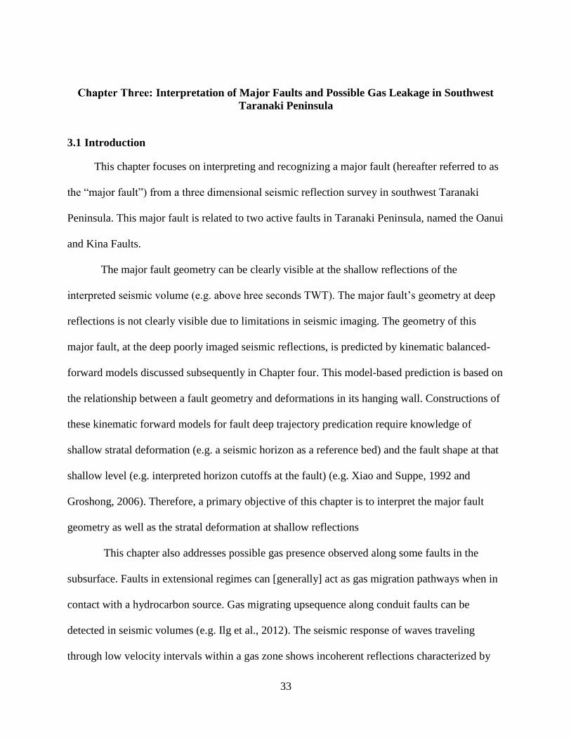
Figure 3-1: (a) Te Kiri 3D survey area in red box, cross-section in Figure 3-2 by green, (b)

Stratigraphic column (after Ilg et al., 2012) .......................................................................... 35

Figure 3-2: Time slice at 810 ms. Steeper dipping tilted fault blocks appear as narrower

reflections than shallower dipping beds (green). Amplitude termination at reflection

discontinuities indicates fault locations on a horizontal slice (yellow). ............................... 40

Figure 3-4: A sequence of consecutive horizontal TWT sections. The NE-trending major

fault (black dashed line) and its associated secondary synthetic fault (green dashed line). . 41

Figure 3-5: Examples of gas flow along normal faults in the southern Taranaki Basin

(after Ilg et al., 2012). Vertical scale is in seconds TWT. A) and B) Cone-shape

amplitude distortions along normal faults C) and D) Bright spots and reflectivity loss ....... 45

Figure 3-6: Interpretation of gas reflections on a vertical section. Possible gas flow pathway

is indicated in bright red (appears as cone-shape incoherence). In green, estimated top

Eocene sandstone reservoir which had hydrocarbon shows in Te Kiri-1 well. (modified

after Alarfaj and Lawton, 2012) ............................................................................................ 46

Figure 3-7: Horizontal section of semblance attribute at 810 ms TWT. Low semblance

clearly delineate fault locations shown as amplitude terminations on Figure 3-3. ............... 48

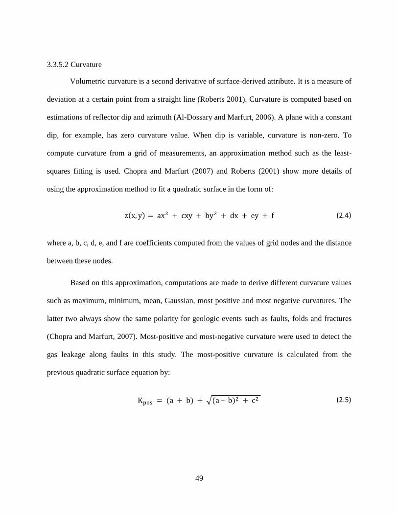
Figure 3-8: Horizontal section of most-positive curvature at 810 ms TWT. ................................ 50

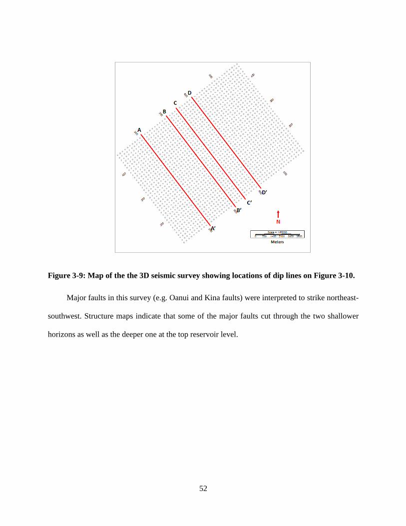
Figure 3-9: Map of the the 3D seismic survey showing locations of dip lines on Figure 3-10. ... 52

ix

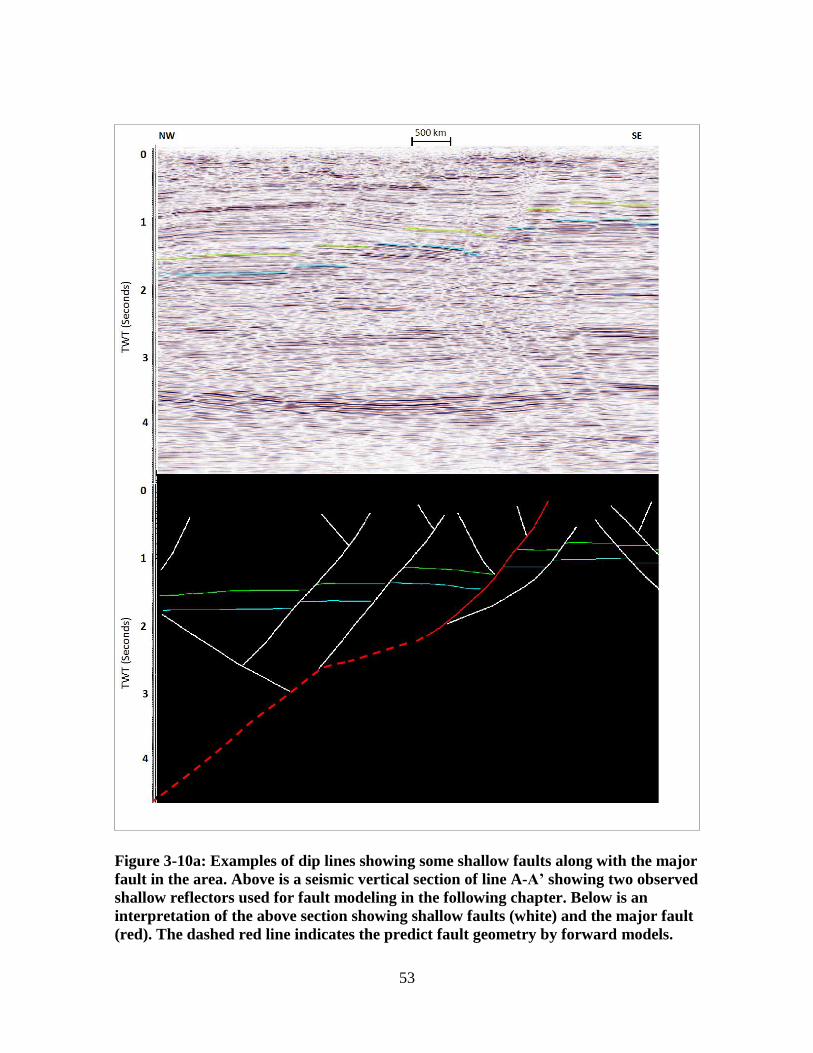
Figure 3-10a: Examples of dip lines showing some shallow faults along with the major fault

in the area. Above is a seismic vertical section of line A-A’ showing two observed

shallow reflectors used for fault modeling in the following chapter. Below is an

interpretation of the above section showing shallow faults (white) and the major fault

(red). The dashed red line indicates the predict fault geometry by forward models............. 53

Figure: 3-10: Distribution of low semblance (light blue) superimposed on amplitude sections.

These values predict the location of leakage-like response. Higher semblance values

were filtered (transparent). Leaking normal fault (purple) was interpreted to cut through

the top of reservoir (black) and two other interpreted horizons (blue and green). ............... 60

Figure 3-11: High values of most-positive curvature (red) overlaid on amplitude sections.

These values predict the location of leakage-like response. Lower curvature values were

filtered (transparent). Leaking normal fault (purple) was interpreted to cut through the

top of reservoir (black) and two other interpreted horizons (blue and green). ..................... 61

Figure 3-12: multi-attributes overlaid on vertical and horizontal amplitude sections to predict

leakage locations. Filtered values are shown for semblance (light blue), most positive

curvature (red) and most negative curvature (yellow). The more attributes shown within

the same locality, the higher is the chance for gas presence. ................................................ 62

Figure 4-1: A movement over a concave-upward fault bend causes hanging-wall strata to

collapse instantaneously along an active axial surface to fill a void created by extension.

(a) Pre-faulting state (b) Void created by extension (c) The active axial surface is pinned

at the FWC of the fault bend (d) Deformed beds (grey) after passing through the active

axial surface. ......................................................................................................................... 69

Figure 4-2: (a)-(e) Sequential stages of deformation over a concave-upward fault bend. Grey

lines indicate deformed hanging-wall beds within a kink band. ........................................... 72

Figure 4-3: (a)-(e) Sequential stages of deformation over a convex-upward fault bend. Grey

lines indicate deformed hanging-wall beds within a kink band. ........................................... 75

Figure 4-4: (a)-(d) Sequential stages of deformation of syntectonic deposition over a concave

bend. White horizons indicate growth sediments. Grey lines indicate deformed hanging-

wall beds within a kink band................................................................................................. 79

Figure 4-5: Sensitivity to changes in antithetic shear angles: a) 30o b) 25o c) 20o d) 15o e) 10o .. 82

Figure 4-6: Kinematic forward modeling for fault prediction on a depth converted seismic

section. Light green and blue are interpreted seismic horizons. Dark green and blue are

modeled horizons. The interpreted major fault shape is shown in red (solid line). The

dashed red lines indicate the dip domain of secondary faults at fault bends ........................ 88

Figure 4-7: Incorrect model showing deformation caused by a listric fault ................................. 97

10

Introduction

1.1 Overview

Exploration and development of hydrocarbons trapped in Earth require knowledge of the

subsurface structure and stratigraphy. Interpretations of the ‘unseen’ subsurface are based on

direct and indirect methods at different scales of investigation. Interpreters must then integrate

different types of data (geophysical, geological, and petrophysical) to achieve a better model that

estimates the subsurface geology. In geophysical prospecting, reflection seismology remains a

primary tool for imaging and predicting the subsurface geology.

One of the main objectives of this thesis is to analyze and model faulting patterns from a

seismic reflection volume in an extensional regime. This chapter introduces basic concepts of the

seismic response of acoustic waves propagating through the subsurface as well as covers the

outlines and objectives of this thesis.

1.2 Seismic Interpretation

Interpretation of seismic reflection data is a fundamental tool for finding and developing

oil and gas prospects. Reflection seismology is an indirect measurement tool which provides

meaningful information used to construct reliable models of the subsurface. Seismic

interpretation is subject to the data quality which is significantly affected by the acquisition and

processing parameters of the seismic survey.

Advancements and efforts in seismic data acquisition and processing are aimed to

improve the quality and interpretability of seismic data. While seismic acquisition and

processing are based on mathematical principles and handled mainly digitally, seismic

interpretation remains primarily a visual process (e.g. based on intellectual correlation, pattern

11

recognition… etc), used to describe the subsurface geology and define the size and position of

hydrocarbon targets (Herron, 2011).

Unlike acquisition and processing which are considered a forward process, seismic

interpretation is considered an inverse process that can provide different explanations to a

particular dataset (i.e. non-unique solutions) (Yilmaz, 2001; Herron, 2011). Therefore, seismic

interpretation must be a model-driven process based on sound geologic principles.

A fundamental fact that has to be kept in an interpreter’s mind is that seismic reflection

data is an estimation of the subsurface, measured in two way travel time (TWT), and is not an

exact representation of the true subsurface geology. The seismic response to the earth’s layers

and structure is constrained with limitations that should be addressed during the interpretation

process.

1.2.1 Seismic Response

Seismic data is acquired when sensors detect the reflected sound waves (or echoes)

generated from a seismic source (e.g. explosives or vibroseis). Sound waves propagate and

spread out though the subsurface causing vibrations along rocks and fluids they pass through.

When seismic waves encounter a geological boundary between two different earth’s layers, some

of the waves are reflected (i.e. travel back to the surface) and some are transmitted (i.e. continue

to propagate further in earth).

Vibrations arriving to the sensors at the surface are detected and recorded as a function of

time. The output result is the seismic trace, which typically consists of the time break at the

initiation of the seismic source, then the first arrival or first break which is caused by waves

propagating along the earth surface (e.g. not reflected), followed by reflections caused by the

12

acoustic waves bouncing off boundaries between different earth layers. The primary reflections

in the seismic trace would ideally represent the Earth’s layers in the subsurface. The strength of a

reflected wave typically decreases with increasing time.

Geoscientists generally employ variables extracted from seismic data to describe different

Earth properties. These variables are velocity (compressional Vp and shear Vs), density (ρ) and

absorption (Q) (Yilmaz, 2001). Wave velocities determine the propagation paths and travel

times. Velocities along with densities define the acoustic impedance in seismic data.

1.2.2 Seismic Attenuation

Frequencies in seismic data are subject to absorption due to the natural attenuation

property of earth’s materials (Yilmaz, 2001). This attenuation is frequency-dependent and mostly

affects the high-frequency portion of the induced signal. The frequency absorption results in

amplitude decay and decrease in the seismic signal strength with increasing depth (Yilmaz,

2001). With increasing travel-time (or depth), the absorption results in a decrease in the strength

of the source signal and also in amplitude decay. This explains the time-variant nature of the

seismic source wavelet, as its shape and bandwidth vary with time. In addition, acoustic

velocities increase with depth and cause further amplitude decay as waves propagate through

deeper earth layers. The frequency attenuation and amplitude decay significantly deteriorate

seismic resolution of at depth.

1.2.3 Seismic Resolution

Resolution of seismic reflection data determines the ability to resolve or detect two

separate reflecting points on a reflector (i.e. recognizing the two reflecting points as two instead

of one). The minimum distance necessary to image two separate points defines seismic

13

resolution. This is related to the sampling rate of seismic data and affect both temporal and

spatial limits.

The temporal resolution of seismic reflection data determines the minimum thickness

required for a subsurface feature to be adequately imaged in the seismic data (Widess, 1973).

The temporal resolution is controlled by the dominant wavelength (λ), which is determined by

the wave velocity and dominant frequency (e.g. Yilmaz, 2001; Lines and Newrick, 2004):

𝜆 =𝑣

𝑓 (1.1)

where v is wave velocity and f is the dominant frequency.

The dominant frequency is variable both vertically and laterally in seismic data. The

minimum distance necessary for two reflecting points to be recognized in seismic imaging is

about one-fourth of the dominant wavelength (λ/4) (e.g. Yilmaz, 2001; Lines and Newrick,

2004). This resolution limit means that an imaged fault (e.g. a reflector discontinuity) is only

recognized when the fault’s throw is equal to or greater than a quarter of the dominant

wavelength (λ/4). The dominant frequency of acoustic waves traveling through the subsurface

ranges from 20 to 50 Hz and typically decreases with increasing depth. In contrast, seismic

velocities range from 2000 to 5000 m/s and generally increase as acoustic waves propagate

deeper in the subsurface. Subsequently, the typical values of frequencies and velocities can be

used to estimate the possible values of seismic wavelengths which range from 40 to 250 m. The

dominant wavelength generally increases with depth and therefore the resolution and quality of

seismic images typically decreases with increasing depth.

The spatial resolution of seismic reflection data determines how close two points can be

located laterally on a reflector and still be recognized as two separate reflecting points (Lindsey,

14

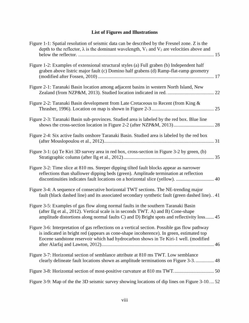
1989). Spatial resolution can be described by an area known as the Fresnel zone (Figure 1-1)

(Sheriff, 1980). Reflections points located within the Fresnel zone are beyond the lateral

resolution limit and therefore are not distinguishable in the seismic image. The Fresnel Zone can

be a measure for seismic spatial resolution. The smaller the Fresnel zone, the smaller the distance

between two differentiable reflecting points and therefore the higher the spatial resolution of the

seismic data. The area of the Fresnel zone is dependent on the seismic wavelength and increases

with depth:

𝑟 = √𝑍 𝜆

2 (1.2)

where Z is the depth to the reflector in meters. The Fresnel zone increases with higher wave

velocities and can be expressed in terms of the dominant frequency (f):

𝑟 = 𝑣

2√

𝑇𝑊𝑇

𝑓 (1.3)

where TWT is two-way travel time of propagating waves (Herron, 2011). This previous equation

indicates that the higher the frequency content, the smaller the size of the Fresnel zone, and

therefore the higher the spatial resolution of seismic data. The size of Fresnel zone is one of the

field parameters considered in seismic acquisition design since it is related to focusing seismic

reflections at targeted depths (Lines and Newrick, 2004).

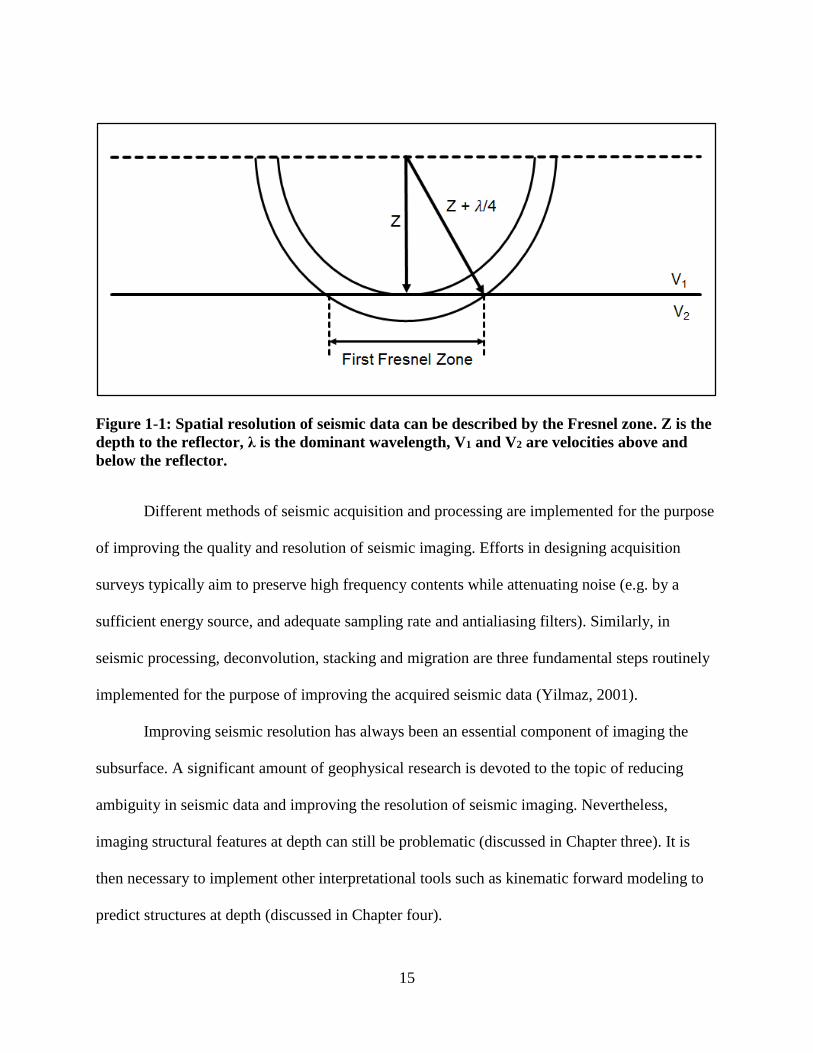
15

Figure 1-1: Spatial resolution of seismic data can be described by the Fresnel zone. Z is the

depth to the reflector, λ is the dominant wavelength, V1 and V2 are velocities above and

below the reflector.

Different methods of seismic acquisition and processing are implemented for the purpose

of improving the quality and resolution of seismic imaging. Efforts in designing acquisition

surveys typically aim to preserve high frequency contents while attenuating noise (e.g. by a

sufficient energy source, and adequate sampling rate and antialiasing filters). Similarly, in

seismic processing, deconvolution, stacking and migration are three fundamental steps routinely

implemented for the purpose of improving the acquired seismic data (Yilmaz, 2001).

Improving seismic resolution has always been an essential component of imaging the

subsurface. A significant amount of geophysical research is devoted to the topic of reducing

ambiguity in seismic data and improving the resolution of seismic imaging. Nevertheless,

imaging structural features at depth can still be problematic (discussed in Chapter three). It is

then necessary to implement other interpretational tools such as kinematic forward modeling to

predict structures at depth (discussed in Chapter four).

16

Interpretation of the subsurface from clear seismic images should be based on sound

geological principles. Therefore, knowledge of tectonic settings and geologic history of an area

is necessary prior to undertaking any seismic interpretation project. The studied region in this

thesis, Taranaki Basin, is currently undergoing extension (King and Thrasher, 1996) and

therefore is expected to exhibit extensional structural features in the subsurface.

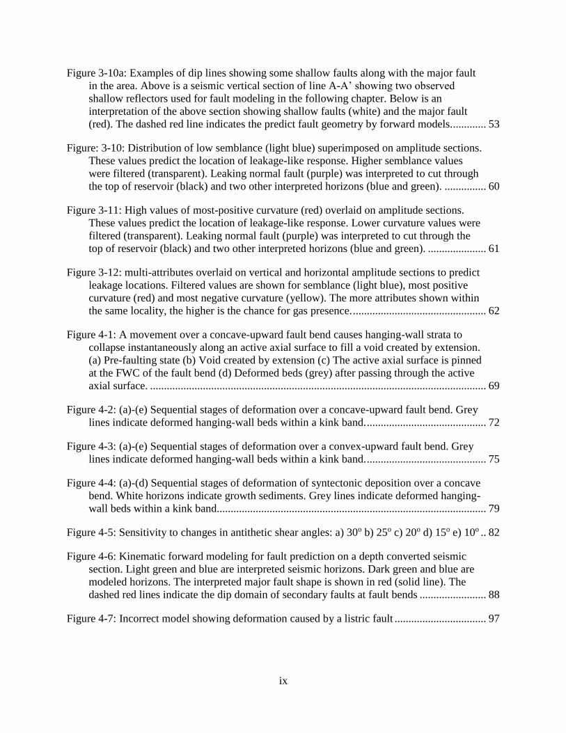
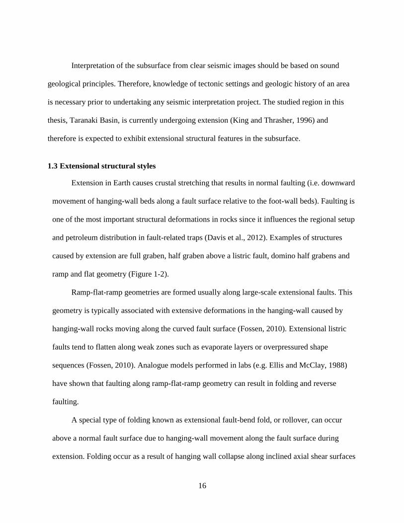
1.3 Extensional structural styles

Extension in Earth causes crustal stretching that results in normal faulting (i.e. downward

movement of hanging-wall beds along a fault surface relative to the foot-wall beds). Faulting is

one of the most important structural deformations in rocks since it influences the regional setup

and petroleum distribution in fault-related traps (Davis et al., 2012). Examples of structures

caused by extension are full graben, half graben above a listric fault, domino half grabens and

ramp and flat geometry (Figure 1-2).

Ramp-flat-ramp geometries are formed usually along large-scale extensional faults. This

geometry is typically associated with extensive deformations in the hanging-wall caused by

hanging-wall rocks moving along the curved fault surface (Fossen, 2010). Extensional listric

faults tend to flatten along weak zones such as evaporate layers or overpressured shape

sequences (Fossen, 2010). Analogue models performed in labs (e.g. Ellis and McClay, 1988)

have shown that faulting along ramp-flat-ramp geometry can result in folding and reverse

faulting.

A special type of folding known as extensional fault-bend fold, or rollover, can occur

above a normal fault surface due to hanging-wall movement along the fault surface during

extension. Folding occur as a result of hanging wall collapse along inclined axial shear surfaces

17

at fault bends. Xiao and Suppe (1992) and other researchers have shown how the geometry of a

normal fault surface can be predicted in the subsurface based on the shape of the hanging wall

of that normal fault. The application of this geometrical relationship between a normal fault and

its deformed hanging-wall layers can serve as powerful prediction tool for structural

interpretation in extensional settings.

Figure 1-2: Examples of extensional structural styles (a) Full graben (b) Independent half

graben above listric major fault (c) Domino half grabens (d) Ramp-flat-ramp geometry

(modified after Fossen, 2010)

1.4 Dataset

The dataset used in this study is provided by the New Zealand Petroleum and Minerals

(NZP&M), which manages the New Zealand Crown Mineral Estate (oil, gas, coal and mineral

resources). A compiled open-file report system along with an extensive exploration and

production data are provided by the New Zealand’s oil and gas industry for public accessible

under the Crown Minerals Act 1991 Section 90 of the New Zealand’s Ministry of Economic

18

Development. This includes seismic and well data along with compiled open-file reports

database (data.nzpam.govt.nz).

1.4.1 Seismic data

The seismic reflection survey used in this study is Te Kiri 3D. This seismic reflection

survey is located southwest Mountain Taranaki, onshore Taranaki Peninsula. Te Kiri 3D survey

was acquired after predictions of commercial prospectivity in the area after drilling the

exploration well, Te Kiri-1, which shows presence of oil and gas in the Miocene- and Eocene-

aged reservoir sequences (Todd Energy, 2006).

1.4.2 Well data

The main well data used in this study are from two exploration wells, Te Kiri-1 and

Te Kiri-2. Both wells are located within the Te Kiri 3D seismic survey. Well data (e.g. checkshot

survey, reference depths, wireline logs, and deviation survey) were used to load the data on the

workstation and tie the seismic reflection data to the well data. Both seismic and well data were

loaded into the KINGDOM Suite for quality check and interpretation.

1.5 Thesis Objectives

The main objective of this thesis is to interpret the geometry of a major fault in a 3D

seismic volume. Interpretations are then related to the geological history and tectonic settings of

the region to assure that results are validated based on geologic principles. A particular interest is

given to interpretation of the major fault and seismic horizons at shallow reflections which are

required for the second objective of this thesis.

19

The second objective of this thesis is to construct kinematic structural forward models for

the major fault in the 3D seismic volume to predict the fault’s trajectory at deep reflections

where the fault trace is not clearly visible. The kinematic forward models are based on principles

related to the extensional fault-bend fold theory. Modeling the major fault in the interpreted

seismic volume reveals the geometry of the fault surface, which cuts through the proven gas

reservoir in the subsurface and possibly contributes to the gas presence observed along the

interpreted fault.

The third objective of this thesis is to analyze the possible gas presence associated with

normal faults in the seismic volume. The interpretation of the fault-related gas leakage in the

survey is undertaken using different volumetric seismic attributes.

1.6 Thesis Outline

Chapter two covers the geologic background of The basin’s history. It discusses the

tectonic kinematics and explains the evolution of Taranaki Basin through geologic times. The

chapter links the deformation mechanisms in the subsurface to potential hydrocarbon traps.

This chapter discusses the contribution of tectonic activities to the faulting patterns and

subsurface structure since the initiation of Taranaki Basin in the mid-Cretaceous.

Chapter three shows interpretation of the major fault in the seismic volume and relate it

to two active faults previously studied on Taranaki Peninsula. The chapter discusses the quality

of the seismic images and shows horizons interpretation from the 3D seismic reflection survey.

This chapter also addresses the possible gas presence along normal faults predicted in the

seismic images. The chapter explains the gas effect on the seismic reflections, and defines

different seismic attributes used for predicting the possible gas presence along normal faults.

20

Chapter four shows the created kinematic forward models and explains the main concepts

behind the created models. The chapter describes how the geometry of a normal fault is related

to strain in its hanging wall and show the use of the models to predict fault geometries at poorly

imaged deep reflections.

Chapter five summarizes the results and discusses the conclusions of this thesis.

1.7 Software

The following software was used for my work on this research project:

KINGDOM® Suite: for geological and geophysical interpretation of seismic and well data

Rock Solid AttributesTM: for computation of geometric attributes from seismic data

StructureSolverTM: for balanced forward models of deformation associated with faults

Microsoft® Office: for spreadsheet, word processing and image editing

21

Geological Background of Taranaki Basin

2.1 Introduction

The primary objective of this chapter is to provide a background for the geologic history

of Taranaki Basin, New Zealand. Deformation in the subsurface of Taranaki Basin is linked to

the tectonic kinematics, which explains the basin’s evolution through geologic time.

Understanding these deformation mechanisms is essential for targeting potential structures

trapping hydrocarbon in the subsurface. This chapter provides an overview of the tectonic setting

since the initiation of the basin in the mid-Cretaceous. Subsequently, the chapter discusses the

contribution of these tectonic activities to the faulting patterns and subsurface structure in the

basin.

2.2 Background

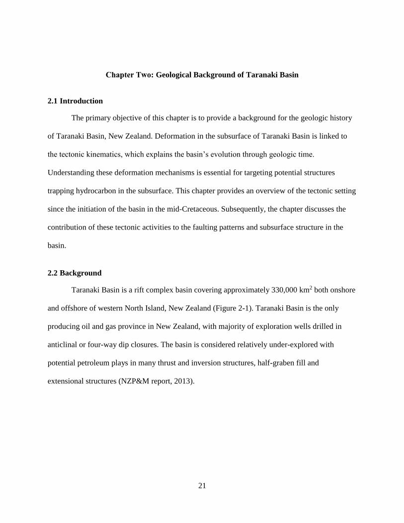
Taranaki Basin is a rift complex basin covering approximately 330,000 km2 both onshore

and offshore of western North Island, New Zealand (Figure 2-1). Taranaki Basin is the only

producing oil and gas province in New Zealand, with majority of exploration wells drilled in

anticlinal or four-way dip closures. The basin is considered relatively under-explored with

potential petroleum plays in many thrust and inversion structures, half-graben fill and

extensional structures (NZP&M report, 2013).

22

Figure 2-1: Taranaki Basin location among adjacent basins in western North Island, New

Zealand (from NZP&M, 2013). Studied location indicated in red.

23

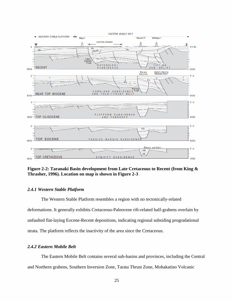
2.3 Tectonic Settings

Taranaki Basin is located on the active boundary of the Australian and Pacific tectonic

plates and has undergone different phases of deformation. The Taranaki Basin was part of the

Pacific Plate during the basin’s early evolution. Mid-Cretaceous comprises a pre-rift/break-up

phase followed by extension and left-lateral shear, contributing to the initiation of the basin and

marking a phase of syn-rift and drift during the Late Cretaceous to Paleocene (Figure 2-2).

The basin then has undergone a passive margin phase during post-rift/drift Paleocene-

Early Oligocene times, which involved a subsidence in the eastern part of the basin. A renewed

episode of subsidence started in mid-Oligocene in central areas of the basin and an overall

subsidence influenced the basin during Oligocene to Early Miocene times (ranges from about

500-2000 m) (King and Thrasher, 1996). Subsidence during Oligocene was associated with

westward downthrow of Taranaki Fault in the eastern limit of the basin (King and Thrasher,

1996).

Taranaki Basin evolved as an east active and west passive margins, separated by the

western limit of the Australian-pacific boundary. The active part is referred to as the Eastern

Mobile Belt (or the “Taranaki Graben”) and the inactive margin is referred to as the Western

Stable Platform (Figure 2-3). Even though areas such as the Taranaki Peninsula experienced

uplift at some period during the Neogene, rapid subsidence beginning mid-Oligocene contributed

to an overall net subsidence in the Eastern Mobile Belt. The overall subsidence in the east

exceeded the relatively undeformed Western Stable Platform which remained mostly inactive

since the Cretaceous.

The basin also experienced a deformation phase of contraction in late Eocene to Miocene,

involving a major horizontal compression during early Miocene in the eastern part of the basin.

24

In the Early Miocene, the Taranaki basin was subject to the changing converging plate boundary

during which the Taranaki Fault overthrust westwardly, resulting in a reverse upward movement

of the basement by up to 6 km in the eastern limit of the basin.

During Pliocene to Pleistocene, the basin deformed along the plate boundary in the

eastern part of the basin and resulted in major areas of extension. This Plio-Pleistocene extension

has contributed to an overall net subsidence in the basin, except for the eastern uplifted and tilted

areas, and the southern inversion region.

2.4 Subsurface Structure

The basin’s subsurface structure is significantly influenced by the tectonic history of the

basin and directly related to deformations along the Australian-Pacific plate boundary. As

previously mentioned, the structure of the Basin consists of two main regions, the Western Stable

Platform (passive margin) and the Eastern Mobile Belt (active margin) (King, 1991; King et al.,

1991; King and Thrasher 1996). Deformation is mainly characterized by extension and

compression, which are both evident in the Eastern Mobile Belt. The border between these two

regions is marked by the western limit of the current Australian-pacific plate boundary. The

complex tectonic activities resulted in various structural styles in Taranaki Basin, including

normal and reverse faulting along with structural inversion, contained within superimposed sub-

basins, depocentres, and uplifted regions.

25

Figure 2-2: Taranaki Basin development from Late Cretaceous to Recent (from King &

Thrasher, 1996). Location on map is shown in Figure 2-3

2.4.1 Western Stable Platform

The Western Stable Platform resembles a region with no tectonically-related

deformations. It generally exhibits Cretaceous-Paleocene rift-related half-grabens overlain by

unfaulted flat-laying Eocene-Recent depositions, indicating regional subsiding progradational

strata. The platform reflects the inactivity of the area since the Cretaceous.

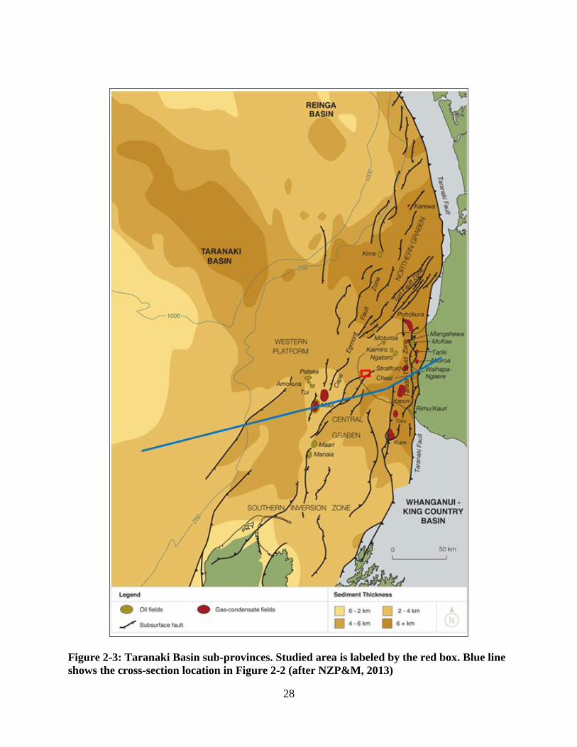
2.4.2 Eastern Mobile Belt

The Eastern Mobile Belt contains several sub-basins and provinces, including the Central

and Northern grabens, Southern Inversion Zone, Tarata Thrust Zone, Mohakatino Volcanic

26

Centre and the Toru Trough. The studied area is located at western Taranaki Peninsula which is

part of the Central Graben. The subsurface structure in the Eastern Mobile Belt resembles the

complex history of the basin’s evolution and deformations related to the Kaikoura Orogeny (e.g.

Suggate et al. 1978 and King & Thrasher, 1996).

Different types of deformation occurred in the Eastern Mobile Belt throughout different

geologic times resulting in complex faulting patterns. Even though strike-slip deformations may

have affected areas in the basin, most offsets are due to dip-slip faults striking mainly to the

north and northeast (e.g. Voggenreiter, 1993; King and Thrasher, 1996). Many of these north-

trending originated during the rifting phase in Late Cretaceous and were then reactivated during

the Cenozoic. The northeast faults were mainly active during the late Cenozoic time, whereas

northeast-trending normal faults in the southwest part of the basin were the result of the Late

Cretaceous rifting. The Late Cretaceous structure consists of fault-controlled sub-basins

resembling an oblique extension zone during the Taranaki Rift (Thrasher 1990b, 1992a).

The Eastern Mobile Belt is bounded in the eastern-most limit by the Miocene age

Taranaki Fault, extending for more than 250 km and truncating younger Miocene layers (King

and Thrasher, 1996). The Taranaki Fault is a major reverse fault dipping eastward and has

contributed to the basin’s structure, vertically shifting the basement by up to 6 km (King and

Thrasher, 1996). The Taranaki Fault along with adjacent subparallel reverse faults to the east

form the Taranaki Fault zone, have increasingly uplifted the basement on the east side of the

fault.

Paleogene structure shows evidence of normal faulting in Paleocene representing the

final stage of early basin rift and generally undisrupted strata during the Eocene. Structure during

Oligocene indicates rapid subsidence, mostly east of the basin.

27

During Neogene, the Eastern Mobile Belt was part of the deformational processes related

to the converging Australian-Pacific plate boundary. In the central part of the Eastern Mobile

Belt, deformation was the result of compression during Miocene followed by extension overlap.

The subsurface structure of the Eastern Mobile Belt indicates an overall net subsidence,

including uplifted areas such as the Taranaki peninsula which experienced reverse faulting

during Miocene along with normal faulting during Pliocene to Recent times. In the northern part

of the basin, the subsurface is deformed mainly by Late Miocene-Recent normal faulting which

represents the western limit of the plate-boundary deformation (i.e. the Cape Egmont Fault

Zone). In the south of Taranaki Basin, the subsurface structure of the Eastern Mobile Belt hosts

Miocene-Recent reverse faults along with structural inversion. King and Thrasher (1994)

classified deformation during Neogene in the Eastern Mobile Belt based on two different stress

regimes:

1. The northern sector (currently under extension), including the Northern and Central

Grabens.

2. The southern sector (have undergone compression): the Tarata Thrust Zone and the

Southern Inversion Zone (southern part still is still under compression).

28

Figure 2-3: Taranaki Basin sub-provinces. Studied area is labeled by the red box. Blue line

shows the cross-section location in Figure 2-2 (after NZP&M, 2013)

29

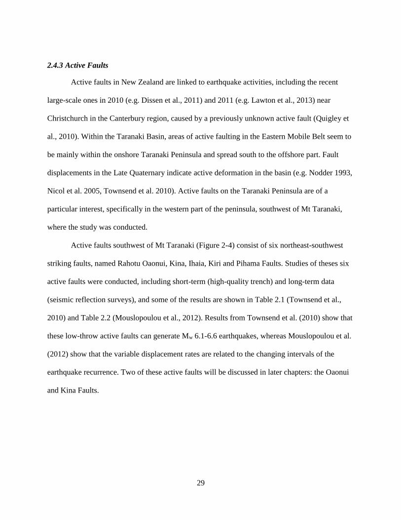
2.4.3 Active Faults

Active faults in New Zealand are linked to earthquake activities, including the recent

large-scale ones in 2010 (e.g. Dissen et al., 2011) and 2011 (e.g. Lawton et al., 2013) near

Christchurch in the Canterbury region, caused by a previously unknown active fault (Quigley et

al., 2010). Within the Taranaki Basin, areas of active faulting in the Eastern Mobile Belt seem to

be mainly within the onshore Taranaki Peninsula and spread south to the offshore part. Fault

displacements in the Late Quaternary indicate active deformation in the basin (e.g. Nodder 1993,

Nicol et al. 2005, Townsend et al. 2010). Active faults on the Taranaki Peninsula are of a

particular interest, specifically in the western part of the peninsula, southwest of Mt Taranaki,

where the study was conducted.

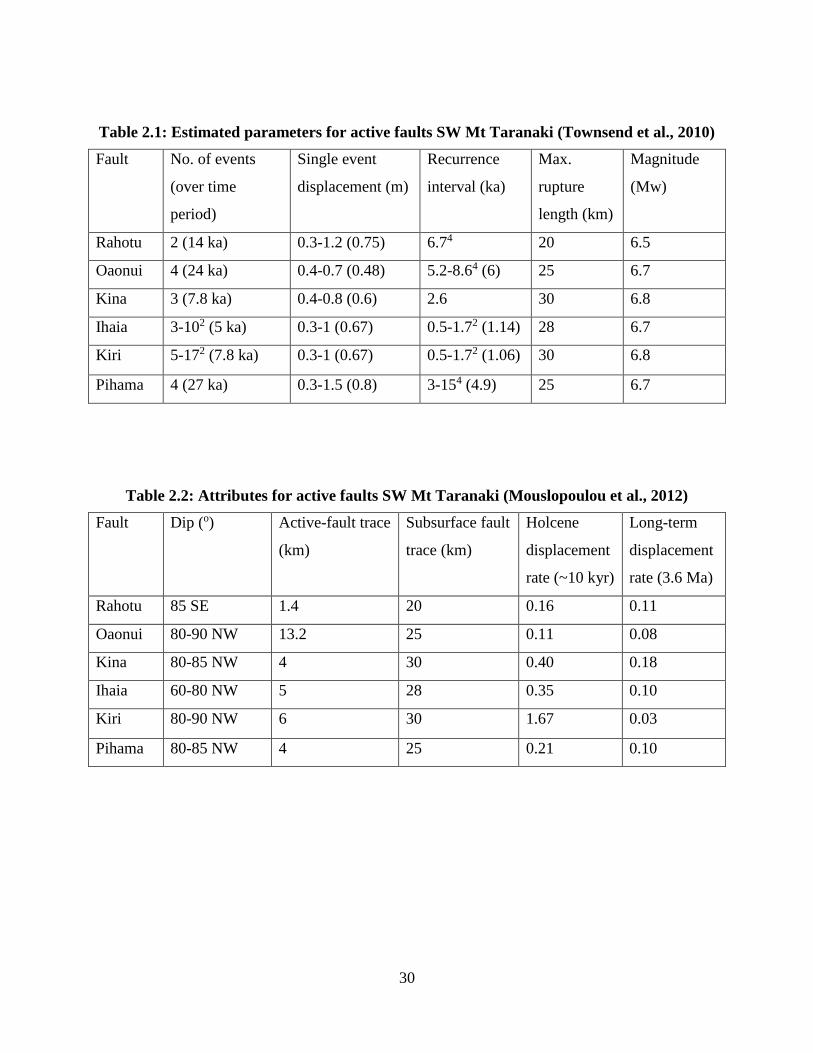
Active faults southwest of Mt Taranaki (Figure 2-4) consist of six northeast-southwest

striking faults, named Rahotu Oaonui, Kina, Ihaia, Kiri and Pihama Faults. Studies of theses six

active faults were conducted, including short-term (high-quality trench) and long-term data

(seismic reflection surveys), and some of the results are shown in Table 2.1 (Townsend et al.,

2010) and Table 2.2 (Mouslopoulou et al., 2012). Results from Townsend et al. (2010) show that

these low-throw active faults can generate Mw 6.1-6.6 earthquakes, whereas Mouslopoulou et al.

(2012) show that the variable displacement rates are related to the changing intervals of the

earthquake recurrence. Two of these active faults will be discussed in later chapters: the Oaonui

and Kina Faults.

30

Table 2.1: Estimated parameters for active faults SW Mt Taranaki (Townsend et al., 2010)

Fault No. of events

(over time

period)

Single event

displacement (m)

Recurrence

interval (ka)

Max.

rupture

length (km)

Magnitude

(Mw)

Rahotu 2 (14 ka) 0.3-1.2 (0.75) 6.74 20 6.5

Oaonui 4 (24 ka) 0.4-0.7 (0.48) 5.2-8.64 (6) 25 6.7

Kina 3 (7.8 ka) 0.4-0.8 (0.6) 2.6 30 6.8

Ihaia 3-102 (5 ka) 0.3-1 (0.67) 0.5-1.72 (1.14) 28 6.7

Kiri 5-172 (7.8 ka) 0.3-1 (0.67) 0.5-1.72 (1.06) 30 6.8

Pihama 4 (27 ka) 0.3-1.5 (0.8) 3-154 (4.9) 25 6.7

Table 2.2: Attributes for active faults SW Mt Taranaki (Mouslopoulou et al., 2012)

Fault Dip (o) Active-fault trace

(km)

Subsurface fault

trace (km)

Holcene

displacement

rate (~10 kyr)

Long-term

displacement

rate (3.6 Ma)

Rahotu 85 SE 1.4 20 0.16 0.11

Oaonui 80-90 NW 13.2 25 0.11 0.08

Kina 80-85 NW 4 30 0.40 0.18

Ihaia 60-80 NW 5 28 0.35 0.10

Kiri 80-90 NW 6 30 1.67 0.03

Pihama 80-85 NW 4 25 0.21 0.10

31

Figure 2-4: Six active faults onshore Taranaki Basin. Studied area is labeled by the red box

(after Mouslopoulou et al., 2012)

2.5 Summary

Taranaki Basin consists of complex subsurface structure resulting from various tectonic

activities from mid-Cretaceous to Recent. Different types of deformation characterize the basin’s

structure, specifically in the eastern region. Most faults in the basin are north- or northeast-

trending. Many of these extensional faults are associated with the Late Cretaceous rifting and

were reactivated during Cenozoic. The basin experienced post-rift contraction and regional

subsidence during Eocene to Early Oligocene.

32

The basin has evolved within two tectonic settings: active eastern margin and passive

western margin. These two tectonic settings resulted in two structural regions: the Eastern

Mobile Belt (active margin) and the Western Stable Platform (passive margin). The Eastern

Mobile Belt experienced a net subsidence during Neogene where as the Western Stable Platform

has been relatively inactive since the Cretaceous.

The Eastern Mobile Belt can be classified into a northern sector, including the Northern

and Central Grabens, and southern sector, including Tarata Thrust Zone and the Southern

Inversion Zone. Within the Central Graben, six north-east trending active faults are known

southwest of Taranaki peninsula: Rahotu Oaonui, Kina, Ihaia, Kiri and Pihama.

33

Interpretation of Major Faults and Possible Gas Leakage in Southwest

Taranaki Peninsula

3.1 Introduction

This chapter focuses on interpreting and recognizing a major fault (hereafter referred to as

the “major fault”) from a three dimensional seismic reflection survey in southwest Taranaki

Peninsula. This major fault is related to two active faults in Taranaki Peninsula, named the Oanui

and Kina Faults.

The major fault geometry can be clearly visible at the shallow reflections of the

interpreted seismic volume (e.g. above hree seconds TWT). The major fault’s geometry at deep

reflections is not clearly visible due to limitations in seismic imaging. The geometry of this

major fault, at the deep poorly imaged seismic reflections, is predicted by kinematic balanced-

forward models discussed subsequently in Chapter four. This model-based prediction is based on

the relationship between a fault geometry and deformations in its hanging wall. Constructions of

these kinematic forward models for fault deep trajectory predication require knowledge of

shallow stratal deformation (e.g. a seismic horizon as a reference bed) and the fault shape at that

shallow level (e.g. interpreted horizon cutoffs at the fault) (e.g. Xiao and Suppe, 1992 and

Groshong, 2006). Therefore, a primary objective of this chapter is to interpret the major fault

geometry as well as the stratal deformation at shallow reflections

This chapter also addresses possible gas presence observed along some faults in the

subsurface. Faults in extensional regimes can [generally] act as gas migration pathways when in

contact with a hydrocarbon source. Gas migrating upsequence along conduit faults can be

detected in seismic volumes (e.g. Ilg et al., 2012). The seismic response of waves traveling

through low velocity intervals within a gas zone shows incoherent reflections characterized by

34

vertical chaotic patterns. Seismic attributes such as semblance and curvature can assist in

detecting gas presence and highlighting locations of the associated permeable faults.

Interpretation of the studied 3D seismic survey was performed using different display

orientations, picking modes and computed seismic attributes.

3.2 Seismic Survey: Te Kiri 3D

3.2.1 Background

The 3D seismic volume used in this study is the Te Kiri 3D which is located onshore,

southwest Mt. Taranaki on the Taranaki Peninsula, New Zealand (Figure 3-1a). Sediments in the

area, similar to other parts of the Taranaki Basin, are of late Cretaceous age and younger (Figure

3-1b). The main objective of this survey, when it was undertaken, was to achieve a high

resolution image of the targeted reservoir level while maintaining the relative amplitude and long

offset data. Another objective of this survey was to image faulting clearly within and above the

targeted reservoir zone, which was estimated to be at 2.5s TWT.

Te Kiri 3D survey was acquired after predictions of commercial prospectivity in the area

after drilling the exploration well, Te Kiri-1 (Todd Energy, 2006). This well showed indications

of oil and gas presence in the Miocene- and Eocene-aged reservoir sequences.

35

Figure 3-1: (a) Te Kiri 3D survey area in red box, cross-section in Figure 3-2 by green, (b)

Stratigraphic column (after Ilg et al., 2012)

3.2.2 Data Acquisition

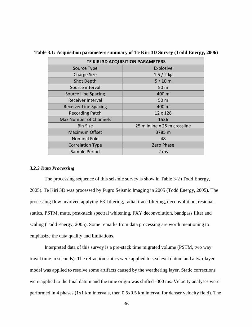
The acquisition parameters for Te Kiri 3D are summarized in Table 3-1 (Todd Energy,

2005). The survey was acquired over an onshore area of 90 sq km. Dynamite was used as the

energy source with a 400 m line spacing. Sensors were aligned orthogonally

(322.6o line-bearing) with 400 m line spacing. The resultant was approximately 4550 shotpoints

on 24 source-lines and 4570 sensor points on 32 receiver-lines. A source interval of 50 m and

receiver interval of 50 m were used resulting in a bin size of 25m x 25m (inline x cross-line).

36

Table 3.1: Acquisition parameters summary of Te Kiri 3D Survey (Todd Energy, 2006)

TE KIRI 3D ACQUISITION PARAMETERS

Source Type Explosive

Charge Size 1.5 / 2 kg

Shot Depth 5 / 10 m

Source interval 50 m

Source Line Spacing 400 m

Receiver Interval 50 m

Receiver Line Spacing 400 m

Recording Patch 12 x 128

Max Number of Channels 1536

Bin Size 25 m inline x 25 m crossline

Maximum Offset 3785 m

Nominal Fold 48

Correlation Type Zero Phase

Sample Period 2 ms

3.2.3 Data Processing

The processing sequence of this seismic survey is show in Table 3-2 (Todd Energy,

2005). Te Kiri 3D was processed by Fugro Seismic Imaging in 2005 (Todd Energy, 2005). The

processing flow involved applying FK filtering, radial trace filtering, deconvolution, residual

statics, PSTM, mute, post-stack spectral whitening, FXY deconvolution, bandpass filter and

scaling (Todd Energy, 2005). Some remarks from data processing are worth mentioning to

emphasize the data quality and limitations.

Interpreted data of this survey is a pre-stack time migrated volume (PSTM, two way

travel time in seconds). The refraction statics were applied to sea level datum and a two-layer

model was applied to resolve some artifacts caused by the weathering layer. Static corrections

were applied to the final datum and the time origin was shifted -300 ms. Velocity analyses were

performed in 4 phases (1x1 km intervals, then 0.5x0.5 km interval for denser velocity field). The

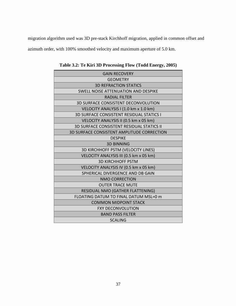
37

migration algorithm used was 3D pre-stack Kirchhoff migration, applied in common offset and

azimuth order, with 100% smoothed velocity and maximum aperture of 5.0 km.

Table 3.2: Te Kiri 3D Processing Flow (Todd Energy, 2005)

GAIN RECOVERY

GEOMETRY

3D REFRACTION STATICS

SWELL NOISE ATTENUATION AND DESPIKE

RADIAL FILTER

3D SURFACE CONSISTENT DECONVOLUTION

VELOCITY ANALYSIS I (1.0 km x 1.0 km)

3D SURFACE CONSISTENT RESIDUAL STATICS I

VELOCITY ANALYSIS II (0.5 km x 05 km)

3D SURFACE CONSISTENT RESIDUAL STATICS II

3D SURFACE CONSISTENT AMPLITUDE CORRECTION

DESPIKE

3D BINNING

3D KIRCHHOFF PSTM (VELOCITY LINES)

VELOCITY ANALYSIS III (0.5 km x 05 km)

3D KIRCHHOFF PSTM

VELOCITY ANALYSIS IV (0.5 km x 05 km)

SPHERICAL DIVERGENCE AND DB GAIN

NMO CORRECTION

OUTER TRACE MUTE

RESIDUAL NMO (GATHER FLATTENING)

FLOATING DATUM TO FINAL DATUM MSL=0 m

COMMON MIDPOINT STACK

FXY DECONVOLUTION

BAND PASS FILTER

SCALING

38

3.3 Data Interpretation Methodology

3.3.1 Horizons interpretation

Interpretation of Te Kiri 3D volume was performed on a workstation using seismic

interpretation software, KINGDOM® Suite SMT. After loading the seismic and well data on the

workstation, a synthetic seismogram was created from Te Kiri-1 well data and tied to the seismic

volume at the well location. The seismic synthetic trace was generated by convolving an

extracted wavelet from the seismic data with the reflection coefficient created by sonic and

density logs. Synthetic seismograms along with formation tops from the well data provide a good

correlation between seismic and well data which help identify the geologic horizons of interest.

Seismic interpretations of the subsurface structure were based on picking horizons along

coherent reflections of the same phase. This usually translates to picks on a peak or trough in

seismic surveys, such as Te Kiri 3D, with zero phase correlation type. These seismic responses

(e.g. peak and troughs) resemble differences in acoustic impedance between different earth

materials. The continuous same-phase reflections are interpreted as horizons representing stratal

surfaces, whereas discontinuities are interpreted to represent fault displacements or

unconformities.

Horizon interpretations of the 3D seismic volume began on vertical sections at the well-

tie location and extended outward. Observations of the seismic images were made on different

display orientations, including horizontal slices, vertical sections of inlines, crosslines and

arbitrary lines.

Horizons were mainly interpreted from seismic reflection amplitudes on vertical sections.

Selected inline and crossline sections were initially analyzed to gain a regional perspective of the

subsurface structure related to the geological history of the area (discussed previously in Chapter

39

two). Alternating between inlines and crosslines served as a validation tool for checking the

consistency of horizons picks along their associated reflectors.

3.3.2 Fault interpretation

Faults can be interpreted in seismic volumes from both vertical and horizontal sections.

Inlines in the studied seismic volume show images along the dominant dip direction and were

interpreted to determine the faulting patterns in the seismic volume. Horizontal sections (i.e. time

or depth slices) were also an integral tool in interpreting the structure in the studied seismic

volume. The horizontal time slices reveal the general orientation of most faults’ strikes. Unlike

vertical sections, the frequency content of horizontal sections is the same as the trace interval in

the data (i.e. spatial sampling) (Yilmaz, 2001). Faults can be observed and interpreted on

horizontal sections. Steeper dipping beds in horizontal slices generally appear as narrower

reflections than shallower dipping beds (Figure 3-2). In addition, reflections of steeper dipping

beds on consecutive time slices appear to change location and move with increasing time (or

depth) faster than shallower dipping beds (Figure 3-3).

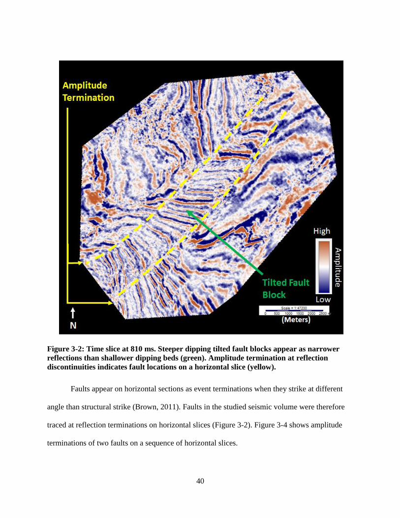
40

Figure 3-2: Time slice at 810 ms. Steeper dipping tilted fault blocks appear as narrower

reflections than shallower dipping beds (green). Amplitude termination at reflection

discontinuities indicates fault locations on a horizontal slice (yellow).

Faults appear on horizontal sections as event terminations when they strike at different

angle than structural strike (Brown, 2011). Faults in the studied seismic volume were therefore

traced at reflection terminations on horizontal slices (Figure 3-2). Figure 3-4 shows amplitude

terminations of two faults on a sequence of horizontal slices.

41

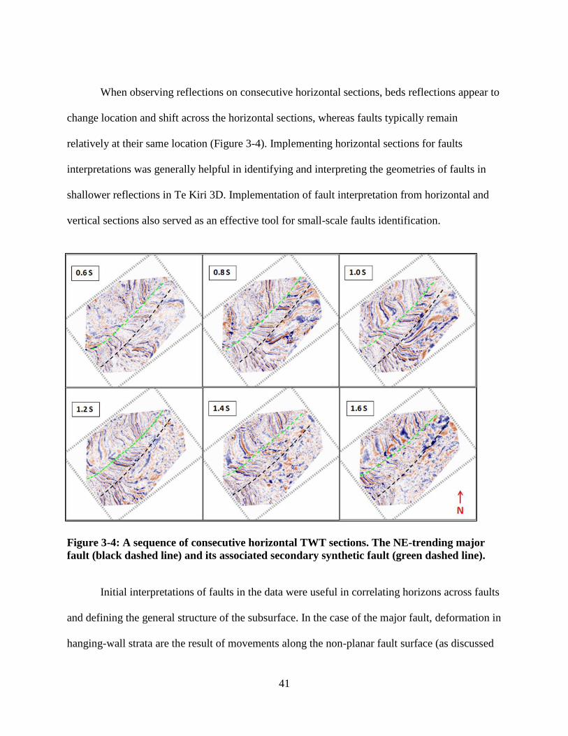
When observing reflections on consecutive horizontal sections, beds reflections appear to

change location and shift across the horizontal sections, whereas faults typically remain

relatively at their same location (Figure 3-4). Implementing horizontal sections for faults

interpretations was generally helpful in identifying and interpreting the geometries of faults in

shallower reflections in Te Kiri 3D. Implementation of fault interpretation from horizontal and

vertical sections also served as an effective tool for small-scale faults identification.

Figure 3-4: A sequence of consecutive horizontal TWT sections. The NE-trending major

fault (black dashed line) and its associated secondary synthetic fault (green dashed line).

Initial interpretations of faults in the data were useful in correlating horizons across faults

and defining the general structure of the subsurface. In the case of the major fault, deformation in

hanging-wall strata are the result of movements along the non-planar fault surface (as discussed

42

later in Chapter four). Interpretation of a fault is therefore helpful in defining the relationship

between the geometry of a fault and the shape of horizons in the hanging wall of that fault.

3.3.3 Fault and Horizon Picking

Seismic interpretation software, KINGDOM® Suite SMT, provides different picking

modes for faults and horizons. These picking modes can be manual, automated, or semi-

automated. Both manual and automated picking were used in interpreting the studied survey.

Manual picking allows for picking data along reflectors regardless of the phase. Fault

surfaces were primarily digitized using manual picking since it provides more control than the

other picking methods. Manual picking was also the basis for horizon picking near faults’

intersections and in complex areas such as narrow fault blocks. Picking closer line spacing was

performed for higher level of details in more complex areas. In areas characterized with good

quality and high amplitude continuity in the shallower reflections, horizon autopicking was

performed for using manual picks as seed points to infill uninterpreted.

When autopicking is performed for a horizon, poor data areas and fault zones were

isolated in map views by polygons. Fault polygons were also used to exclude fault gaps during

the horizon autopicking process. In general, horizon autopicking in Te Kiri 3D volume was

reasonable for shallow reflectors above three seconds.

Interpreted faults in the shallow sections were easily detected and tracked on horizontal

slices using composite sections. Fault picks were then quality controlled to verify that correlated

faults are of the same type, age, and of compatible throw.

Faults are generally indicated by observations of discontinuities or breaks in reflections

(i.e. hanging-wall and footwall cut-offs). Fault picks are then extended upwards and downward

43

until the fault trace is near flexure or invisible. Fault picks were mainly made on inlines (dip

lines) and horizontal sections.

On some interpreted vertical sections, irregular amplitude disturbances were observed at

certain locations where major faults intersect with the interpreted top reservoir. These amplitude

disturbances possibly indicate the presence of gas migrating upward along the interpreted faults.

3.3.4 Gas presence along permeable faults

The presence of gas flowing from faults or fractures might be detected by the acoustic

response in a 3D seismic volume (Ilg et al., 2012). This response can be interpreted qualitatively

in conventional horizontal and vertical sections (Løseth et al., 2009). Gas presence along

permeable faults shows acoustic changes in vertical sections appearing as vertical chaotic

disturbances with amplitude anomalies associated with irregular distribution of low-velocity

zones. This vertical incoherence is a result of scattering, attenuation, and decrease in

compressional velocity (Vp) of waves passing through gas saturated pores (Anderson and

Hampton, 1980). The gas leakage often appears in vertical sections as a cone-shaped distortion

when associated with faults Figure 3-5 (Ilg et al., 2012). When fluids flow upward through

permeable faults, gas molecules are typically released due to the drop in pressure (Bjørkum et. al,

1998). When gas replaces formation water, the contrast of impedance increases and causes the

amplitude variations to show as dim and bright spots. This phenomenon is well-illustrated in

time-lapse studies (e.g. Lawton et. al., 2006 and Alshuhail and Lawton, 2007). The decrease of

P-wave velocity due to gas presence explains the seismic push down often observed within the

leakage zone (Figure 3-6). The velocity drop is due to changes in density and bulk modulus

44

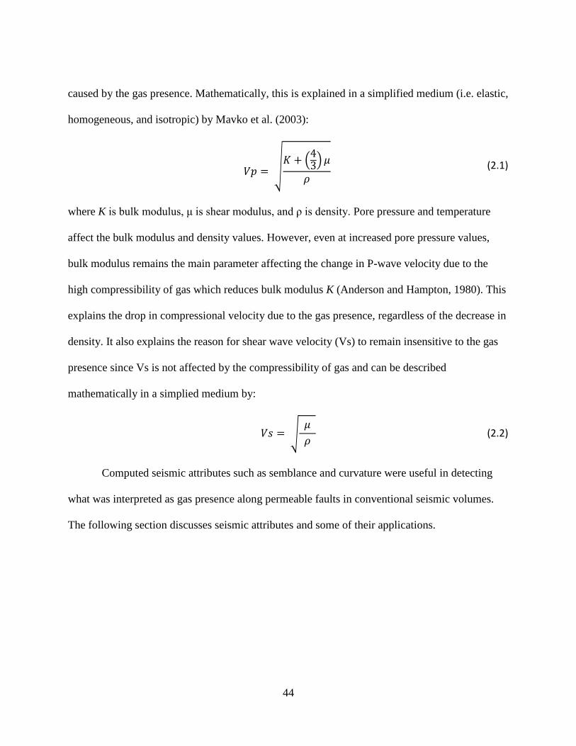
caused by the gas presence. Mathematically, this is explained in a simplified medium (i.e. elastic,

homogeneous, and isotropic) by Mavko et al. (2003):

𝑉𝑝 = √

𝐾 + (43) 𝜇

𝜌

(2.1)

where K is bulk modulus, μ is shear modulus, and ρ is density. Pore pressure and temperature

affect the bulk modulus and density values. However, even at increased pore pressure values,

bulk modulus remains the main parameter affecting the change in P-wave velocity due to the

high compressibility of gas which reduces bulk modulus K (Anderson and Hampton, 1980). This

explains the drop in compressional velocity due to the gas presence, regardless of the decrease in

density. It also explains the reason for shear wave velocity (Vs) to remain insensitive to the gas

presence since Vs is not affected by the compressibility of gas and can be described

mathematically in a simplied medium by:

𝑉𝑠 = √ 𝜇

𝜌 (2.2)

Computed seismic attributes such as semblance and curvature were useful in detecting

what was interpreted as gas presence along permeable faults in conventional seismic volumes.

The following section discusses seismic attributes and some of their applications.

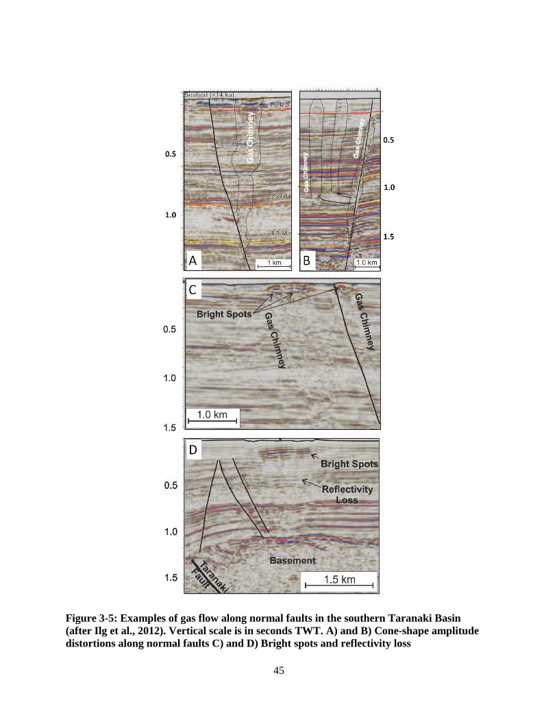
45

Figure 3-5: Examples of gas flow along normal faults in the southern Taranaki Basin

(after Ilg et al., 2012). Vertical scale is in seconds TWT. A) and B) Cone-shape amplitude

distortions along normal faults C) and D) Bright spots and reflectivity loss

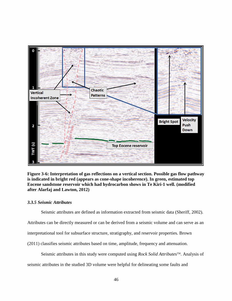
46

Figure 3-6: Interpretation of gas reflections on a vertical section. Possible gas flow pathway

is indicated in bright red (appears as cone-shape incoherence). In green, estimated top

Eocene sandstone reservoir which had hydrocarbon shows in Te Kiri-1 well. (modified

after Alarfaj and Lawton, 2012)

3.3.5 Seismic Attributes

Seismic attributes are defined as information extracted from seismic data (Sheriff, 2002).

Attributes can be directly measured or can be derived from a seismic volume and can serve as an

interpretational tool for subsurface structure, stratigraphy, and reservoir properties. Brown

(2011) classifies seismic attributes based on time, amplitude, frequency and attenuation.

Seismic attributes in this study were computed using Rock Solid AttributesTM. Analysis of

seismic attributes in the studied 3D volume were helpful for delineating some faults and

47

detecting possible gas presence. The most effective attributes are the ones that amplify the

contrast between seismic responses caused by gas reflections and other non-gas related

reflections.

Several useful attributes applied in this study were categorized by Taner (2001) as

geometrical attributes. These attributes scan adjacent traces for each computed trace and describe

the spatial and temporal relationships based on character such as phase, frequency, amplitude,

etc. (Taner, 2001). Examples of these attributes are semblance, curvature, chaotic reflection, dip

variance, dip of maximum similarity, and instantaneous lateral continuity. These attributes are

referred to as “reflective attributes” which correspond to characteristics of interfaces between

two beds. By understanding the characteristic response of acoustic waves passing through gas

zones, leaky faults could be predicted by the output of seismic attributes. Two of seismic

attributes are briefly discussed in the following two sections: semblance and curvature.

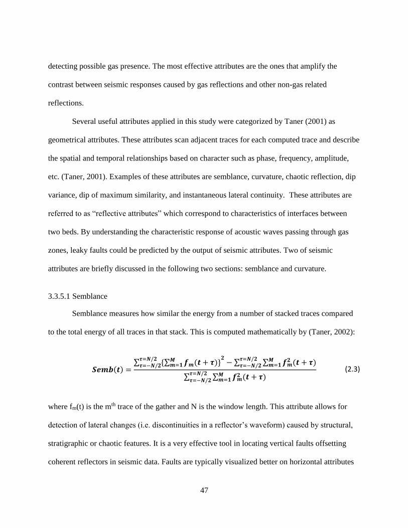
3.3.5.1 Semblance

Semblance measures how similar the energy from a number of stacked traces compared

to the total energy of all traces in that stack. This is computed mathematically by (Taner, 2002):

𝑺𝒆𝒎𝒃(𝒕) =∑ {∑ 𝒇𝒎(𝒕 + 𝝉)}𝑴

𝒎=𝟏𝟐𝝉=𝑵/𝟐

𝝉=−𝑵/𝟐 − ∑ ∑ 𝒇𝒎𝟐 (𝒕 + 𝝉)𝑴

𝒎=𝟏𝝉=𝑵/𝟐𝝉=−𝑵/𝟐

∑ ∑ 𝒇𝒎𝟐 (𝒕 + 𝝉)𝑴

𝒎=𝟏𝝉=𝑵/𝟐𝝉=−𝑵/𝟐

(2.3)

where fm(t) is the mth trace of the gather and N is the window length. This attribute allows for

detection of lateral changes (i.e. discontinuities in a reflector’s waveform) caused by structural,

stratigraphic or chaotic features. It is a very effective tool in locating vertical faults offsetting

coherent reflectors in seismic data. Faults are typically visualized better on horizontal attributes

48

sections. Figure 3-7 shows a horizontal section of semblance at the same time for the horizontal

time slice shown in Figure 3-3. In stratal deformation where continuity of a reflector is

maintained (e.g. fault drag or rollover), no major anomalies are usually shown in computed

semblance.

Figure 3-7: Horizontal section of semblance attribute at 810 ms TWT. Low semblance

clearly delineate fault locations shown as amplitude terminations on Figure 3-3.

49

3.3.5.2 Curvature

Volumetric curvature is a second derivative of surface-derived attribute. It is a measure of

deviation at a certain point from a straight line (Roberts 2001). Curvature is computed based on

estimations of reflector dip and azimuth (Al-Dossary and Marfurt, 2006). A plane with a constant

dip, for example, has zero curvature value. When dip is variable, curvature is non-zero. To

compute curvature from a grid of measurements, an approximation method such as the least-

squares fitting is used. Chopra and Marfurt (2007) and Roberts (2001) show more details of

using the approximation method to fit a quadratic surface in the form of:

z(x, y) = ax2 + cxy + by2 + dx + ey + f (2.4)

where a, b, c, d, e, and f are coefficients computed from the values of grid nodes and the distance

between these nodes.

Based on this approximation, computations are made to derive different curvature values

such as maximum, minimum, mean, Gaussian, most positive and most negative curvatures. The

latter two always show the same polarity for geologic events such as faults, folds and fractures

(Chopra and Marfurt, 2007). Most-positive and most-negative curvature were used to detect the

gas leakage along faults in this study. The most-positive curvature is calculated from the

previous quadratic surface equation by:

Kpos = (a + b) + √(a – b)2 + c2 (2.5)

50

and the most-negative curvature is calculated by:

Kneg = (a + b) − √(a – b)2 + c2 (2.6)

Figure 3-9 shows the most-postive curvature at 810 ms TWT. Note that the most positive values

do not necessarly align with the fault location since curvature is a measurement of bends caused

by and near the fault (rather than a displacement caused by the fault).

Figure 3-8: Horizontal section of most-positive curvature at 810 ms TWT.

51

3.4 Results and Discussion

Te Kiri 3D adequately image the shallow events in the subsurface. Figure 3-9 is a map of

the seismic survey indicating the location of dip lines that are presented as an example to show

some shallow faults along with the major fault in the area (Figure 3-10).

In general, Shallow events in the seismic volume, above three seconds, were clearly

imaged with good signal to noise ratio. Interpretation of seismic images shows normal faulting

dominating the shallow subsurface structure and corresponds to the geologic history of the

region (previously discussed in Chapter two). The quality of data decreases with depth to the

point where faults and horizons are untraceable. During the interpretation process, picks of both

faults and horizons were made based on a geologic model in mind related to the geologic history

of the region (discussed previously in Chapter two).

Figure 3-10 shows three of the interpreted horizons. The shallower horizons were

interpreted to resemble the complex structure at their level and for modeling the major fault

(discussed in chapter four). A deeper horizon was then interpreted to indicate the top of a proven

gas reservoir (productive in Maui gas field) (King and Thrasher, 1996).

52

Figure 3-9: Map of the the 3D seismic survey showing locations of dip lines on Figure 3-10.

Major faults in this survey (e.g. Oanui and Kina faults) were interpreted to strike northeast-

southwest. Structure maps indicate that some of the major faults cut through the two shallower

horizons as well as the deeper one at the top reservoir level.

53

Figure 3-10a: Examples of dip lines showing some shallow faults along with the major

fault in the area. Above is a seismic vertical section of line A-A’ showing two observed

shallow reflectors used for fault modeling in the following chapter. Below is an

interpretation of the above section showing shallow faults (white) and the major fault

(red). The dashed red line indicates the predict fault geometry by forward models.

54

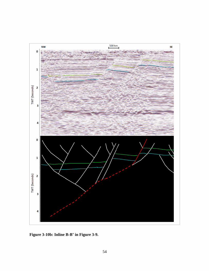
Figure 3-10b: Inline B-B’ in Figure 3-9.

55

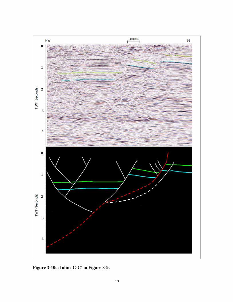
Figure 3-10c: Inline C-C’ in Figure 3-9.

56

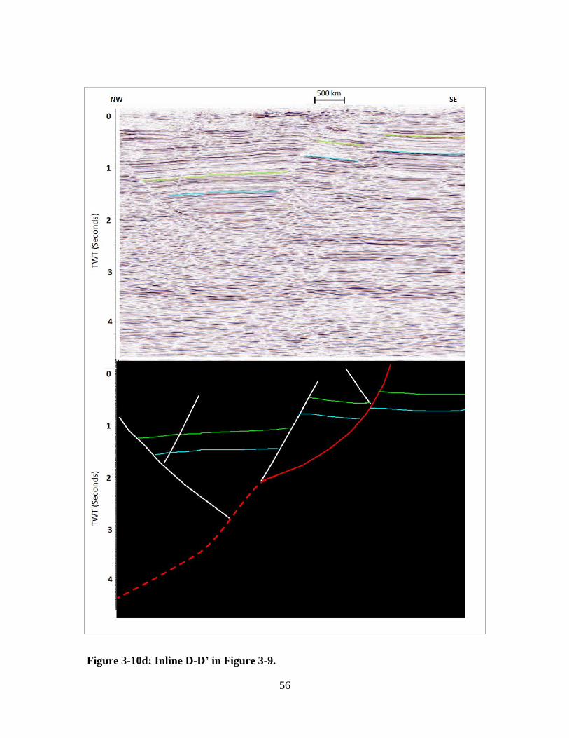
Figure 3-10d: Inline D-D’ in Figure 3-9.

57

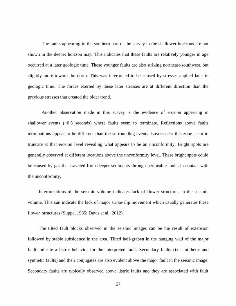
The faults appearing in the southern part of the survey in the shallower horizons are not

shown in the deeper horizon map. This indicates that these faults are relatively younger in age

occurred at a later geologic time. These younger faults are also striking northeast-southwest, but

slightly more toward the north. This was interpreted to be caused by stresses applied later in

geologic time. The forces exerted by these later stresses are at different direction than the

previous stresses that created the older trend.

Another observation made in this survey is the evidence of erosion appearing in

shallower events (~0.5 seconds) where faults seem to terminate. Reflections above faults

terminations appear to be different than the surrounding events. Layers near this zone seem to

truncate at that erosion level revealing what appears to be an unconformity. Bright spots are

generally observed at different locations above the unconformity level. These bright spots could

be caused by gas that traveled from deeper sediments through permeable faults in contact with

the unconformity.

Interpretations of the seismic volume indicates lack of flower structures in the seismic

volume. This can indicate the lack of major strike-slip movement which usually generates these

flower structures (Suppe, 1985; Davis et al., 2012).

The tilted fault blocks observed in the seismic images can be the result of extension

followed by stable subsidence in the area. Tilted half-graben in the hanging wall of the major

fault indicate a listric behavior for the interpreted fault. Secondary faults (i.e. antithetic and

synthetic faults) and their conjugates are also evident above the major fault in the seismic image.

Secondary faults are typically observed above listric faults and they are associated with fault

58

bends (i.e. fault curvature) of an underlying major fault (more details are discussed in Chapter

four).

Poor data quality at depth caused uncertainties in faults interpretation. Figure 3-9b shows

where the faults are not easily traceable at deep reflections. The listric behavior exhibited by the

major fault and its associated hanging-wall deformation leads to questioning whether the major

fault’s dip continues to decrease and flatten out somewhere above the basement, or if it actually

continues to dip steeply and eventually cut through and offset the basement.

Published studies of this studied area show faults interpretation mostly above 3 to 4

seconds TWT. The geometry of the major fault, estimated from the structural kinematic forward

models discussed in Chapter four, shows that the major fault actually continues to dip steeply at

depth. We therefore propose that the major fault in this study is a basement-involved fault and

does not flatten out at a shallower level above the basement (i.e. the major fault cut through the

basement and the overlaying proven reservoir and source rock).

Faults can generally act as part of a hydrocarbon trapping mechanism when in contact

with a hydrocarbon-filled formation. They can act as a migration path when permeable or as a

seal when impermeable. Indications of gas presence along some of the interpreted faults,

including the major fault, are evident in this studied seismic volume.

The presence of fault-related gas leakage is observed on vertical sections. Figure 3-9

shows an example view of the major normal fault cutting through the Eocene reservoir

sequences. Associated with this fault is a zone of disrupted seismic reflections showing the gas

leakage characteristics discussed previously. The root of this leakage zone seems to be originated

59

beneath the Eocene reservoir level. The leakage zone resembles a cone-shape chaotic response

which appears as a zone of vertical incoherence extending almost to the surface. The gas leakage

zone in general appears to exhibit relatively lower amplitude, whereas the top of the zone shows

bright spots. Bright spots are high amplitudes caused by a strong drop in acoustic impedance

and are often considered a direct indicator of gas presence.

The seismic response of the gas leakage zone appear to be distinguished on seismic

attributes (Figure 3-10). The effects of acoustic waves traveling through low velocity gas zones

are shown as disruptions in coherency of the data. This translates to very low semblance values

along the gas leakage zone. Disrupted signals also result in high values of the curvature attribute

(Figure 3-11). This can be due to changes in geometric local dips as a result of scattering within

the gas leakage zone. The dip changes can be evident on dip variance attributes (Figure 3-12).

The gas presence in the seismic volume is observed to fall generally within the extreme

ends of certain attributes’ spectrum. For example, the leakage zone was represented by the

lowest semblance (Figure 3-10) and highest curvature values (Figure 3-11). This can be

particularly useful when it comes to observations for the distribution of possible gas presence

along faults in the survey. When attribute values are analyzed, they can be filtered based on a

certain threshold value by opacity removal. This allows for showing only the seismic attribute

values interpreted to be caused by gas presence along the interpreted faults.

Figure 3-12 show an example of filtered values of overlaid on conventional amplitude

sections. The opacity removal should be determined by analysis of several sections at leakage

zones from different locations and can be overlaid on a horizontal slices to indicate the

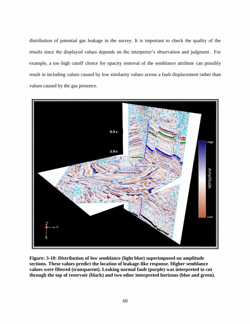
60

distribution of potential gas leakage in the survey. It is important to check the quality of the

results since the displayed values depends on the interpreter’s observation and judgment. For

example, a too high cutoff choice for opacity removal of the semblance attribute can possibly

result in including values caused by low similarity values across a fault displacement rather than

values caused by the gas presence.

Figure: 3-10: Distribution of low semblance (light blue) superimposed on amplitude

sections. These values predict the location of leakage-like response. Higher semblance

values were filtered (transparent). Leaking normal fault (purple) was interpreted to cut

through the top of reservoir (black) and two other interpreted horizons (blue and green).

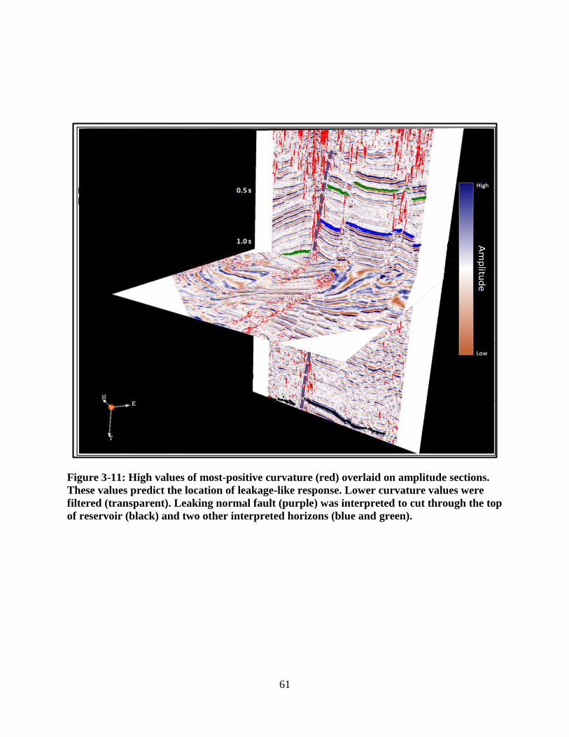
61

Figure 3-11: High values of most-positive curvature (red) overlaid on amplitude sections.

These values predict the location of leakage-like response. Lower curvature values were

filtered (transparent). Leaking normal fault (purple) was interpreted to cut through the top

of reservoir (black) and two other interpreted horizons (blue and green).

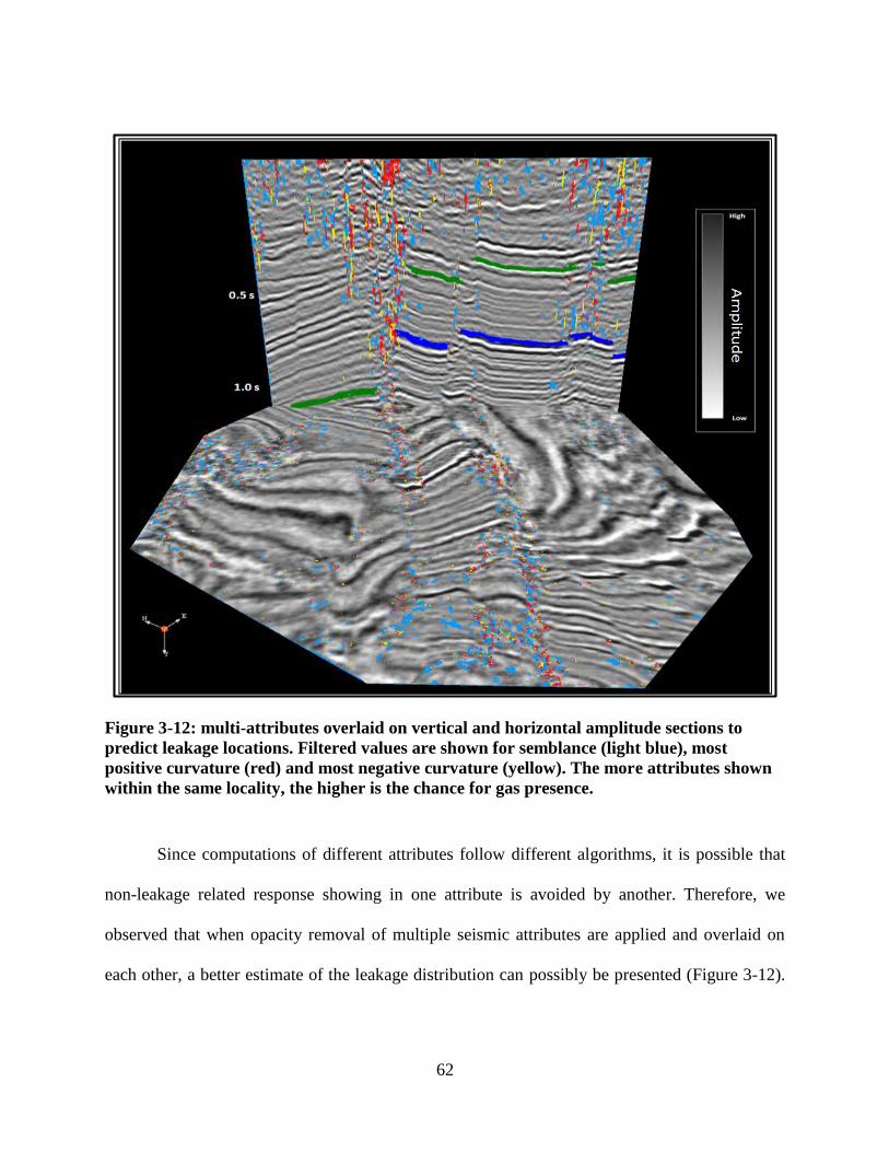
62

Figure 3-12: multi-attributes overlaid on vertical and horizontal amplitude sections to

predict leakage locations. Filtered values are shown for semblance (light blue), most

positive curvature (red) and most negative curvature (yellow). The more attributes shown

within the same locality, the higher is the chance for gas presence.

Since computations of different attributes follow different algorithms, it is possible that

non-leakage related response showing in one attribute is avoided by another. Therefore, we

observed that when opacity removal of multiple seismic attributes are applied and overlaid on

each other, a better estimate of the leakage distribution can possibly be presented (Figure 3-12).

63

More values of different computed attributes shown at a given location can indicate a higher

chance of gas presence at that location.

Utalizing different seisimc attributes can be integrated using neural networks to detect

gas presence in a seismic volume. Meldahl et al, (1998) and Aminzadeh et al (2001) describe a

developed multi-attributes approach for pattern recognition though neural networks. The use of

multi-attributes has proven to be effective in detecting geologic features such as gas chimneys.

This method require several picks for chimney and non-chimney samples. If interpreters have

access to a neural network software, a better estimate is possible for detecting the locations of

gas presence (e.g. seismic gas chimneys).

Deformations associated with faults in the interpreted seismic volume are mainly due to

dip-slip movements rather than strike-slip movements (indicated by the lack of flower structures

in the interpreted seismic volume and from the geologic history of the region previously

discussed in Chapter two). We therefore propose the loss of image across a fault’s cutoffs in the

interpreted seismic volume to be caused by the presence of gas rather than distributed strain

caused by strike-slip movement.

3.5 Summary and Conclusions

Te Kiri 3D reveals a complex structure dominated by normal faults. Major faults are

mapped and shown to be generally striking northeast-southwest. Interpretations of this survey

show evidences of the diverging history of the subsurface. Possible gas leakage is identified

along some of the interpreted faults in Te Kiri 3D. The interpretation of gas presence is

supported by observations of amplitude anomalies and incoherent reflections within the leakage

zone. Attributes such as semblance and curvature are helpful in detecting unique responses

64

caused by gas presence. The opacity removal is a helpful visualization tool that can assist in

detecting and delineating the gas-leakage distribution in the survey.

The evidence of possible gas migrating up-sequence in the seismic image is linked to the

interpreted faults that might cut through a hydrocarbon-filled formation. These faults are

typically not visible at the deeper poorly imaged reflections in the survey. It is therefore essential

to predict a fault’s geometry at depth and determine whether or not that fault is in contact with

the deep proven reservoir.

The geologic history of the region along with the lack of flower structures in the

interpreted seismic volume indicate that deformations associated with faults are mainly due to

dip-slip rather than strike-slip movements. The lost of seismic image across faults’ cutoffs, is

therefore due to the presence of gas rather than distributed strain caused by strike-slip movement.

65

Kinematic Structural Forward Modeling for Fault Trajectory Prediction in

Seismic Interpretation

4.1 Introduction

One of the main objectives of this dissertation is to examine the geometry of normal

faults from seismic images where these faults may not be very visible. In this chapter, we create

kinematic forward models based on the rollover theory of Xiao and Suppe (1992) and

extensional balancing concepts of inclined shear deformation. Implementation and model

development were undertaken using recently released structural modelling software,

STRUCTURESOLVER, made available to this project. All the created models are balanced (i.e.

cross sectional area is preserved). The kinematic forward models describe how the geometry of a

normal fault is related to its hanging-wall strain. Deformation resulting from movement of

hanging-wall block along non-planar normal faults (e.g. listric growth faults) can be analyzed by

generated rollover structures in the downthrown of that non-planar fault.

In this chapter, we address controlling variables affecting hanging-wall deformation,

including the fault geometry, amount of sedimentation, slip ratio and shear angles. We then

create kinematic forward models to estimate the trajectory of the Oaonui Fault at depth where

seismic reflections are poorly imaged.

4.2 Background

Rocks, when undergoing deformation, flow, bend or, in the case of faults, slip. Mapping

faults is crucial in hydrocarbon exploration and production as faults can act as a sealing

mechanism for a potential trap, or a conduit for fluids in tight formations. Faults are inferred in

the subsurface by seismic imaging which is an indirect representation of the subsurface measured

66

in two-way time. Seismic imaging is often associated with signal distortion and limitations in

temporal and spatial resolution. Seismic data may be subject to misinterpretation since it is an

approximation of the subsurface and is at best, only a representation of the true geology.

Interpreted seismic reflections are based on the acoustic seismic response which

resembles differences in impedance between different earth materials. Continuous reflections are

typically interpreted as horizons representing stratal surfaces, whereas discontinuities are

interpreted to represent fault displacements or unconformities. Many efforts have been made to

automate fault tracking based on reflection discontinuities. Examples are algorithms such as

semblance, which is a continuity measurement (Marfurt et al., 1998), variance, a discontinuity

measurement (Randen et al., 2001) and most recently an extraction method based on fault

surface computation and extraction (Hale, 2013). Despite the advancements made in autopicking

algorithms, not all discontinuities are caused by faults. Reflection terminations can be caused by

stratigraphic features such as unconformities or by imaging artifacts (Herron, 2000).

Furthermore, subsurface structures maybe invisible or mis-positioned on imaged sections

(Lawton and Isaac, 2001). As a result, seismic interpretation often requires validation tools to

properly understand the true subsurface structure and generate better prospects.

4.3 Kinematic Structural Forward Modeling of Hanging-wall Rollovers

Kinematic balanced forward models can provide geologically reasonable solutions to

seismic images by extrapolating known data (e.g. well-imaged shallow seismic reflectors) into

ambiguous data (e.g. poorly-imaged deep seismic reflections). Specifically, in extensional

settings, where normal faults dominate the Earth’s crust, inclined simple shear modeling can

predict a distinct relationship between a fault shape and its hanging-wall deformation. This

67

relationship has been analyzed by physical modeling (e.g. Cloos, 1968; McClay and Ellis, 1987)

and quantitative studies (e.g. Gibbs, 1983; White, 1986; Rowan and Kligfield, 1989; Groshong,

1989; Dula, 1992; Nunns, 1991; Xiao and Suppe, 1992). Dula (1991) compared different

algorithms of kinematic modeling showing the inclined-shear model to be the most realistic.

Xiao and Suppe (1992) further explained the concept of how the geometry of a deformed

hanging wall is controlled by the shape of the fault.

Hanging-wall rollover is a type of fault-bend fold, generated by bending of hanging-wall

blocks during movement along fault bends (i.e. nonplanar faults) (Suppe, 1985). Rollover is

sometimes referred to in the literature as reverse drag and typically considered an important

location of hydrocarbon accumulation (Suppe, 1985). The concepts of the rollover define how

hanging-wall strata deform along active axial surfaces by coulomb shear collapse (e.g. Xiao and

Suppe, 1992).

4.3.1 Coulomb Shear Collapse

In extensional tectonic regimes, the hanging-wall block of a planar fault subsides with a

displacement vector parallel to the fault surface. In the case of a non-planar fault consisting of

two fault segments or more, the hanging-wall block is moved by different displacement vectors

during slip. If the hanging-wall block was purely rigid, a void would be created between the

hanging-wall and footwall-wall blocks due movement along the lower fault segment below the

fault bend (e.g. Hamblin 1965, Xiao and Suppe, 1992) (Figure 4-2b). However, in reality, beds

overlaying this void would collapse due to gravitational forces and instantaneously fill the void

(Figure 4-1d). This collapse occurs in the Coulomb shear direction, known the Coulomb collapse

(Suppe 1985 and Xiao and Suppe, 1994), which is dipping 65-70o without the impact of

68

compaction (Xiao and Suppe, 1989). Collapsing hanging-wall beds deform and rollover due to

shearing along active axial surfaces (Figure 4-2c, d). The active axial shear surfaces form at fault

bends and are fixed at depth to the footwall cutoffs of those bends. Collapsing hanging-wall beds

create secondary normal faults parallel to the active axial surfaces and these faults are usually

visible on seismic images.

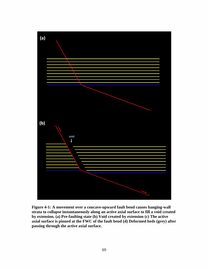
69

Figure 4-1: A movement over a concave-upward fault bend causes hanging-wall

strata to collapse instantaneously along an active axial surface to fill a void created

by extension. (a) Pre-faulting state (b) Void created by extension (c) The active

axial surface is pinned at the FWC of the fault bend (d) Deformed beds (grey) after

passing through the active axial surface.

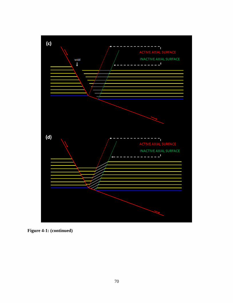
70

Figure 4-1: (continued)

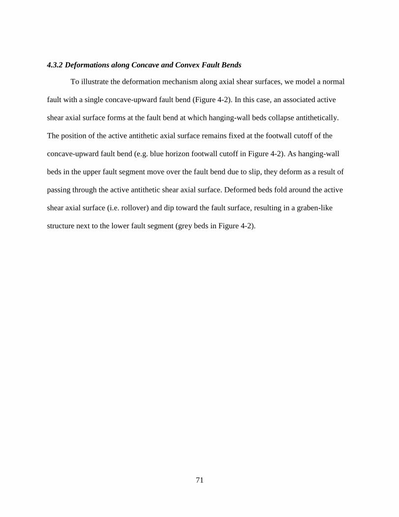
71

4.3.2 Deformations along Concave and Convex Fault Bends

To illustrate the deformation mechanism along axial shear surfaces, we model a normal

fault with a single concave-upward fault bend (Figure 4-2). In this case, an associated active

shear axial surface forms at the fault bend at which hanging-wall beds collapse antithetically.

The position of the active antithetic axial surface remains fixed at the footwall cutoff of the

concave-upward fault bend (e.g. blue horizon footwall cutoff in Figure 4-2). As hanging-wall

beds in the upper fault segment move over the fault bend due to slip, they deform as a result of

passing through the active antithetic shear axial surface. Deformed beds fold around the active

shear axial surface (i.e. rollover) and dip toward the fault surface, resulting in a graben-like

structure next to the lower fault segment (grey beds in Figure 4-2).

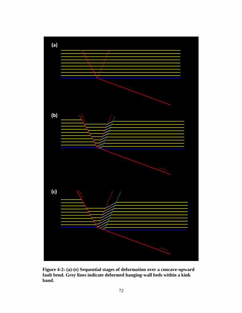
72

Figure 4-2: (a)-(e) Sequential stages of deformation over a concave-upward

fault bend. Grey lines indicate deformed hanging-wall beds within a kink

band.

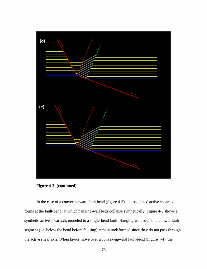
73

Figure 4-2: (continued)

In the case of a convex-upward fault bend (figure 4-3), an associated active shear axis

forms at the fault-bend, at which hanging-wall beds collapse synthetically. Figure 4-3 shows a

synthetic active shear axis modeled in a single-bend fault. Hanging-wall beds in the lower fault

segment (i.e. below the bend before faulting) remain undeformed since they do not pass through

the active shear axis. When layers move over a convex-upward fault-bend (Figure 4-4), the

74

position of the active synthetic axis remains fixed at the footwall cutoff of the fault bend (e.g. the

blue horizon footwall cutoff in figure 4-3), and beds passing over that fault bend collapse

synthetically along the active shear axis causing the beds to dip away from the fault.

The boundary between the deformed and undeformed beds in the lower fault segment

defines the position of an inactive axial surface. This inactive axial surface remains parallel to

the active axial surface in all stages of deformation. In an undeformed state (i.e. prior to

faulting), active and inactive axial surfaces are aligned in the same position at the fault bend

(Figures 4-3a and 4-4a). The inactive shear axial surface terminates in the hanging-wall cutoff at

the fault bend prior to slip and moves with the hanging-wall block along the fault surface during

slip (e.g. blue horizon hanging-wall cutoff at fault bend in Figures 4-3 and 4-4).

75

Figure 4-3: (a)-(e) Sequential stages of deformation over a convex-upward

fault bend. Grey lines indicate deformed hanging-wall beds within a kink

band.

76

Figure 4-3: (continued)

4.3.3 Deformation zone

The active and inactive shear axial surfaces form together a kink band which

encompasses a deformation zone. Suppe (1985) defines this kink band as a discrete zone within

which the beds have been deformed and rotated relative to their geometry outside this zone. The

axial surfaces bounding this deformation zone are called kink-band boundaries.

77

The geometry of kink bands are defined by two angles (Suppe, 1985). The first is the

external kink angle (γ) between the active axial surface and the undeformed beds (i.e. beds that

have not passed through the active axial surface). The second angle is the internal kink angle (γk)

between the deformed layers within the kink band and the active axial surface., the possible

value for the external kink angle (γ) ranges between 0o to 90o and for the internal kink angle (γk)

ranges between 0o and 180o. However, in real Earth structures, Suppe (1985) states that the most

common values for the external kink angle (γ) is between 50 o and 65 o, whereas the internal kink

angle (γk) is typically between 75o and 85o.

The width of this deformation zone within the kink band is proportional to the fault slip

(i.e. the distance between the active and inactive axial surfaces equals the slip along the fault

surface). As slip increases, the deformation zone widens. All deformed beds, which passed

through the active axial surface, are contained within this zone. As hanging-wall layers slip along

the fault surface, new accommodation space is created above subsiding hanging-wall allowing

new sediments to be deposited.

4.3.4 Syn-tectonic Deposition

Deposition during faulting creates growth strata (Figure 4-4). Stratigraphic thicknesses in

the downthrown hanging-wall beds increase in growth faults (i.e. during syn-depostional

processes). The model shows growth beds (white horizons in Figure 4-4) are thickest in the

graben-like structure above the steepest fault segment. Similar to pre-growth beds, growth

deposits start to collapse and deform resulting in a monoclinal rollover as they pass through the

active shear axis, which remains stationary throughout all stages of deformation. In contrast,

growth sediments that did not pass through the active shear axis remain undeformed (i.e.

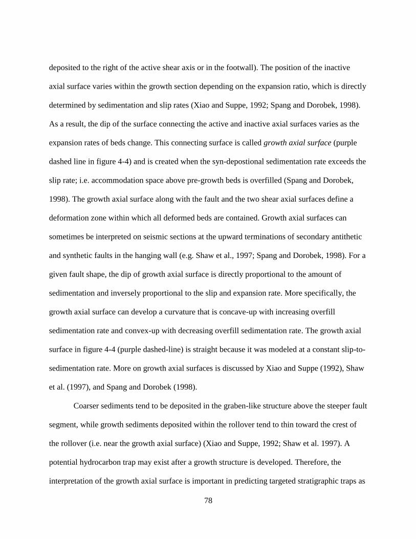
78

deposited to the right of the active shear axis or in the footwall). The position of the inactive

axial surface varies within the growth section depending on the expansion ratio, which is directly

determined by sedimentation and slip rates (Xiao and Suppe, 1992; Spang and Dorobek, 1998).

As a result, the dip of the surface connecting the active and inactive axial surfaces varies as the

expansion rates of beds change. This connecting surface is called growth axial surface (purple

dashed line in figure 4-4) and is created when the syn-depostional sedimentation rate exceeds the

slip rate; i.e. accommodation space above pre-growth beds is overfilled (Spang and Dorobek,

1998). The growth axial surface along with the fault and the two shear axial surfaces define a

deformation zone within which all deformed beds are contained. Growth axial surfaces can

sometimes be interpreted on seismic sections at the upward terminations of secondary antithetic

and synthetic faults in the hanging wall (e.g. Shaw et al., 1997; Spang and Dorobek, 1998). For a

given fault shape, the dip of growth axial surface is directly proportional to the amount of

sedimentation and inversely proportional to the slip and expansion rate. More specifically, the

growth axial surface can develop a curvature that is concave-up with increasing overfill

sedimentation rate and convex-up with decreasing overfill sedimentation rate. The growth axial

surface in figure 4-4 (purple dashed-line) is straight because it was modeled at a constant slip-to-

sedimentation rate. More on growth axial surfaces is discussed by Xiao and Suppe (1992), Shaw

et al. (1997), and Spang and Dorobek (1998).

Coarser sediments tend to be deposited in the graben-like structure above the steeper fault

segment, while growth sediments deposited within the rollover tend to thin toward the crest of

the rollover (i.e. near the growth axial surface) (Xiao and Suppe, 1992; Shaw et al. 1997). A

potential hydrocarbon trap may exist after a growth structure is developed. Therefore, the

interpretation of the growth axial surface is important in predicting targeted stratigraphic traps as

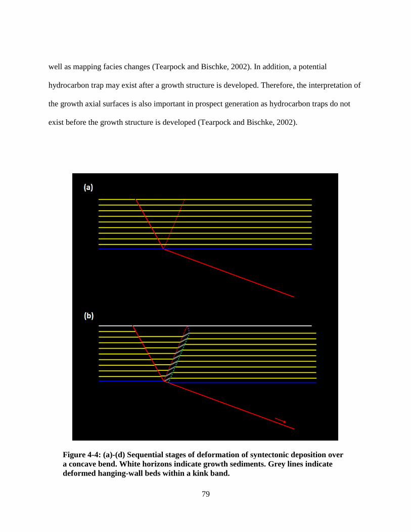
79

well as mapping facies changes (Tearpock and Bischke, 2002). In addition, a potential

hydrocarbon trap may exist after a growth structure is developed. Therefore, the interpretation of

the growth axial surfaces is also important in prospect generation as hydrocarbon traps do not

exist before the growth structure is developed (Tearpock and Bischke, 2002).

Figure 4-4: (a)-(d) Sequential stages of deformation of syntectonic deposition over

a concave bend. White horizons indicate growth sediments. Grey lines indicate

deformed hanging-wall beds within a kink band.

80

Figure 4-4: (continued)

4.3.5 Shear Angles

Another factor affecting the deformation is the shear angles at which beds collapse. The

shear angle is the acute angle between the vertical and the inclined shear axis (White et al.,

1986). The collapse angle is determined from the dip of secondary faults. Figures 4-5 shows the

sensitivity of the deformed beds geometries to shear angles at a concave-upward fault bend. For

81

an antithetic shear axis, the model shows the dip of deformed hanging-wall beds decreases as the

shear angle increases. In contrast, the dip of deformed hanging-wall beds increases as the shear

angle increases for a synthetic shear axis.

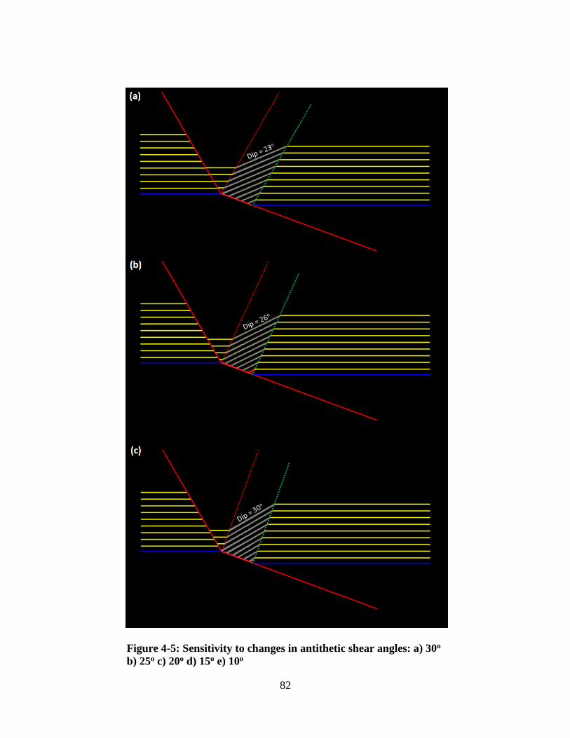
82

Figure 4-5: Sensitivity to changes in antithetic shear angles: a) 30o

b) 25o c) 20o d) 15o e) 10o

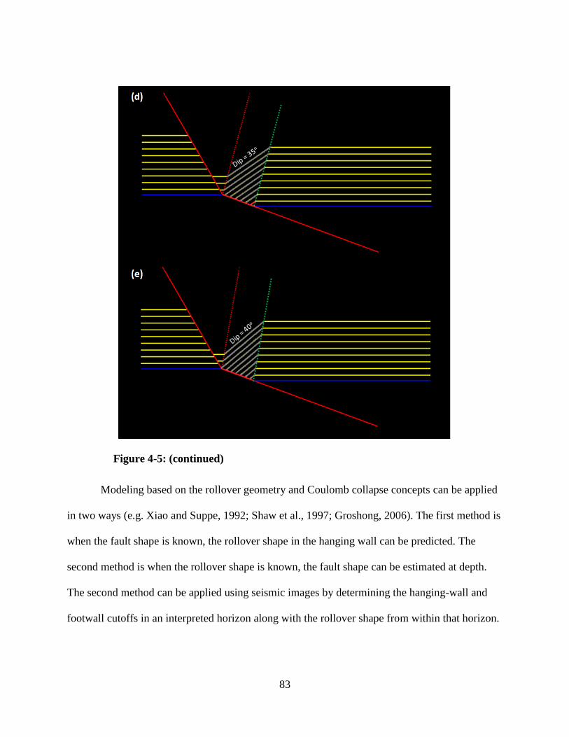
83

Figure 4-5: (continued)

Modeling based on the rollover geometry and Coulomb collapse concepts can be applied

in two ways (e.g. Xiao and Suppe, 1992; Shaw et al., 1997; Groshong, 2006). The first method is

when the fault shape is known, the rollover shape in the hanging wall can be predicted. The

second method is when the rollover shape is known, the fault shape can be estimated at depth.

The second method can be applied using seismic images by determining the hanging-wall and

footwall cutoffs in an interpreted horizon along with the rollover shape from within that horizon.

84

In the next section, we use the second method to create kinematic forward models to predict the

shape of Oaonui Fault at depth from seismic data.

4.4 Modeling Active Oaonui Fault Southwest Taranaki Peninsula

The concepts of extensional fault-bend folding, discussed in the previous sections, are

very practical for assisting in seismic interpretation. We constructed kinematic forward models

based on these concepts to solve for ambiguities in our seismic interpretation of the Oaonui Fault

(as discussed in chapter 3). The models are used to predict the geometry of the fault in deeper

poorly-imaged seismic reflections based on the hanging-wall rollover structures in the shallower

well-imaged reflections.

We modeled the Oaonui Fault from vertical sections in the Te Kiri 3D seismic survey to

investigate the fault’s geometry at depth (below 2.4 seconds TWT). Structural interpretation of

this survey showed north-east trending normal faults dominating the shallow reflections which

can be easily observed by tracing alignments of amplitude terminations on time slices or

converted depth slices. These observations of amplitude terminations indicate the geometry of

the fault surface in the strike direction. Computed volumetric attributes (e.g. based on semblance

and variance algorithms) were helpful in delineating the shallow fault surfaces in the survey, but

not in the deeper poorly imaged seismic sections (Chapter 3).

The Oaonui Fault exhibits listric characteristics with its thickening hanging-wall blocks

tilting toward the fault surface. The listric-like shape implies that the fault’s dip continues to

decrease gradually until it flattens out at depth. However, the exact fault shape is difficult to trace

at deep reflections below about 2.6 seconds (TWT).

85

The Oaonui Fault was previously interpreted by Townsend et al. (2010) as one of the

main active faults in Taranaki Peninsula. However, Townsend et al. (2010) does not show an

interpretation of the fault’s geometry below 3 seconds reflection TWT.

As explained in the previous sections, deformations are mostly the result of collapsing

hanging-wall beds along active axial surfaces associated with the fault bends. We model the

Oaonui fault by incorporating our interpretation of the fault bends along with the dip angles of

active axial surfaces which are indicated by secondary faults.

Kinematic forward models based on seismic images must be constructed on sections

parallel to the dominant dip direction. Therefore, we used vertical sections from Te Kiri 3D

seismic survey that are perpendicular to the interpreted strike direction of the Oaonui Fault to

construct the kinematic forward models in this study.

Figure 4-6a is a time migrated seismic section parallel to the dip of Oaonui Fault which is

shown in red in the middle of the section. We model the Oaonui Fault based on knowledge of its

shape at the well-imaged shallow reflections and horizon cutoffs at the fault surface. The

interpreted horizons are of Early Pliocene (green) and Late Miocene (Blue) (Figure 4-6). The

brighter green and blue horizons in Figure 4-6 indicate the interpreted horizons of the observed

beds geometry in the seismic reflections in the section. Secondary antithetic and synthetic faults

are observed in the hanging wall of the fault to indicate the dip domain and orientation of the

active shear axial surfaces as well as the shear angles. The fault shape is therefore modeled by

series of fault bends; concave-upward bends at deep terminations of antithetic faults and convex-

upward bends at deep terminations of synthetic faults with the fault. Adjusting the shape of the

modeled fault changes the geometry of the modeled hanging-wall beds (darker green and blue) .

The modeled hanging-wall beds (darker green and blue) in Figure 4-6 are matched with the

86

interpreted seismic horizons (brighter green and blue) to validate the model and confirm the

fault’s shape.

We also modeled different scenarios for the fault geometry at the poor deep reflections in

the section to verify our model-based seismic interpretation. One of the modeled scenarios is a

listric shape that flattens out at shallower reflections above about 3.2 seconds (TWT). We

examined each scenario by varying the fault shape at depth while trying to match the modeled

hanging-wall horizons with the ones interpreted from the seismic sections (Figure 4-7). A

mismatch between the modeled and observed horizons indicates an incorrect fault geometry.

4.5 Results and Discussion

The modeled geometry of Oaonui Fault adequately resembles the well-imaged seismic

reflections of the interpreted shallow structure. The models suggest that the deformations in the

hanging-wall structure were mainly controlled by movements along the underlying Oaonui Fault

surface. The bends in Oaonui Fault were constructed to match the interpreted fault trace and. The

fault trace below 3 seconds (TWT) is not clearly visible, and therefore the fault bends were

inferred by secondary faults.

Some of the antithetic faults observed on the seismic section do not connect to their

associated fault bends. Instead, these antithetic faults terminate downward at the position of a

major synthetic fault associated with an active axial surface originating at a convex bend in the

modeled fault. This case is observed in many growth faults (Tearpock and Bischke, 2002).

Nevertheless, the dip domain of these antithetic faults can be used to construct concave bend for

in the modeled fault. The dips of secondary faults observed on the seismic sections are generally

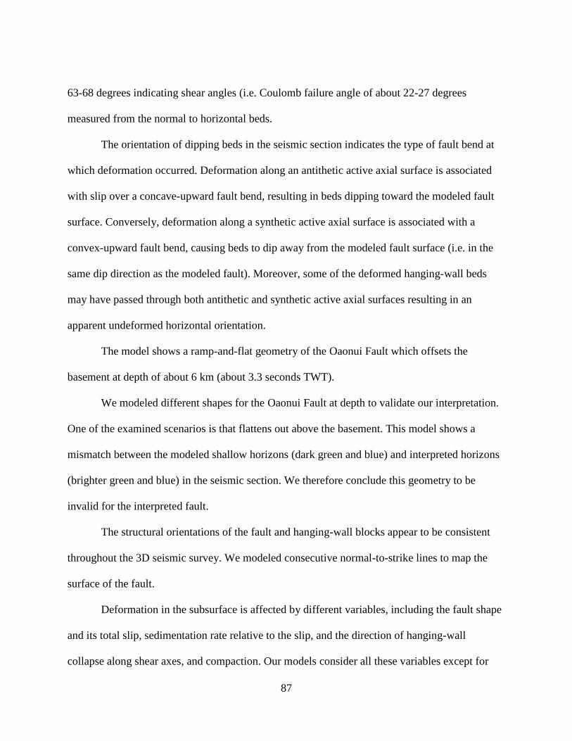
87

63-68 degrees indicating shear angles (i.e. Coulomb failure angle of about 22-27 degrees

measured from the normal to horizontal beds.

The orientation of dipping beds in the seismic section indicates the type of fault bend at

which deformation occurred. Deformation along an antithetic active axial surface is associated

with slip over a concave-upward fault bend, resulting in beds dipping toward the modeled fault

surface. Conversely, deformation along a synthetic active axial surface is associated with a

convex-upward fault bend, causing beds to dip away from the modeled fault surface (i.e. in the

same dip direction as the modeled fault). Moreover, some of the deformed hanging-wall beds

may have passed through both antithetic and synthetic active axial surfaces resulting in an

apparent undeformed horizontal orientation.

The model shows a ramp-and-flat geometry of the Oaonui Fault which offsets the

basement at depth of about 6 km (about 3.3 seconds TWT).

We modeled different shapes for the Oaonui Fault at depth to validate our interpretation.

One of the examined scenarios is that flattens out above the basement. This model shows a

mismatch between the modeled shallow horizons (dark green and blue) and interpreted horizons

(brighter green and blue) in the seismic section. We therefore conclude this geometry to be

invalid for the interpreted fault.

The structural orientations of the fault and hanging-wall blocks appear to be consistent

throughout the 3D seismic survey. We modeled consecutive normal-to-strike lines to map the

surface of the fault.

Deformation in the subsurface is affected by different variables, including the fault shape

and its total slip, sedimentation rate relative to the slip, and the direction of hanging-wall

collapse along shear axes, and compaction. Our models consider all these variables except for

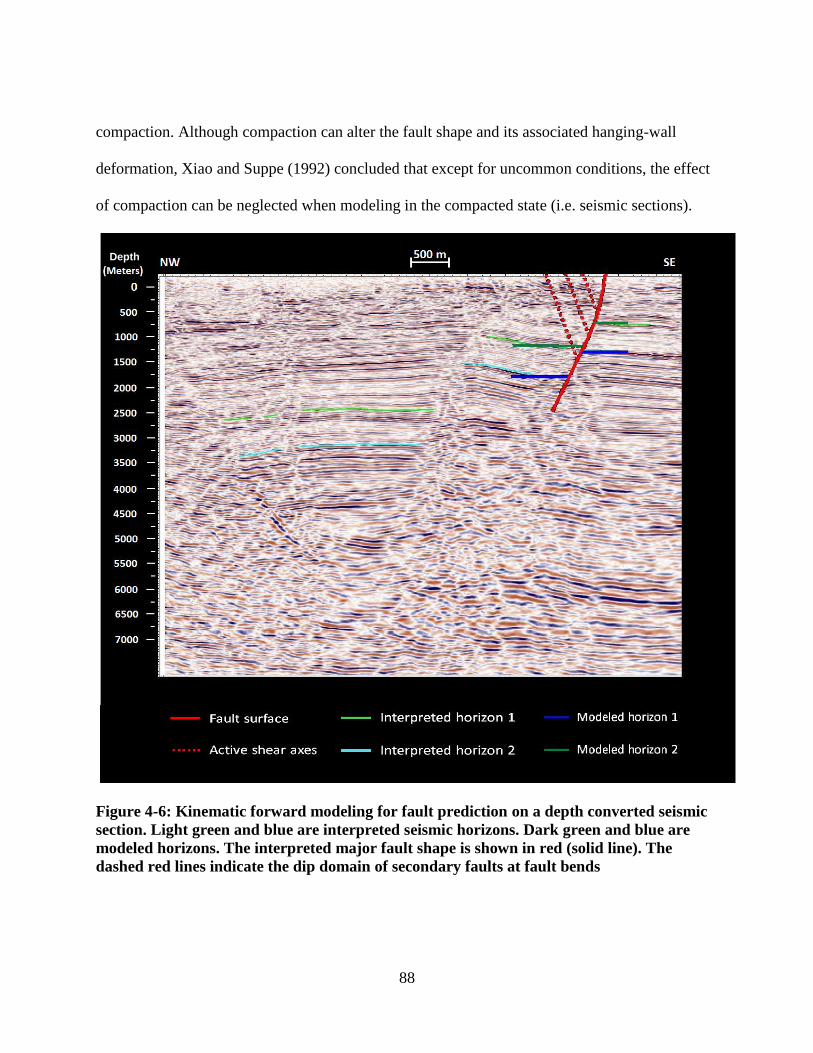
88

compaction. Although compaction can alter the fault shape and its associated hanging-wall

deformation, Xiao and Suppe (1992) concluded that except for uncommon conditions, the effect

of compaction can be neglected when modeling in the compacted state (i.e. seismic sections).

Figure 4-6: Kinematic forward modeling for fault prediction on a depth converted seismic

section. Light green and blue are interpreted seismic horizons. Dark green and blue are

modeled horizons. The interpreted major fault shape is shown in red (solid line). The

dashed red lines indicate the dip domain of secondary faults at fault bends

Depth

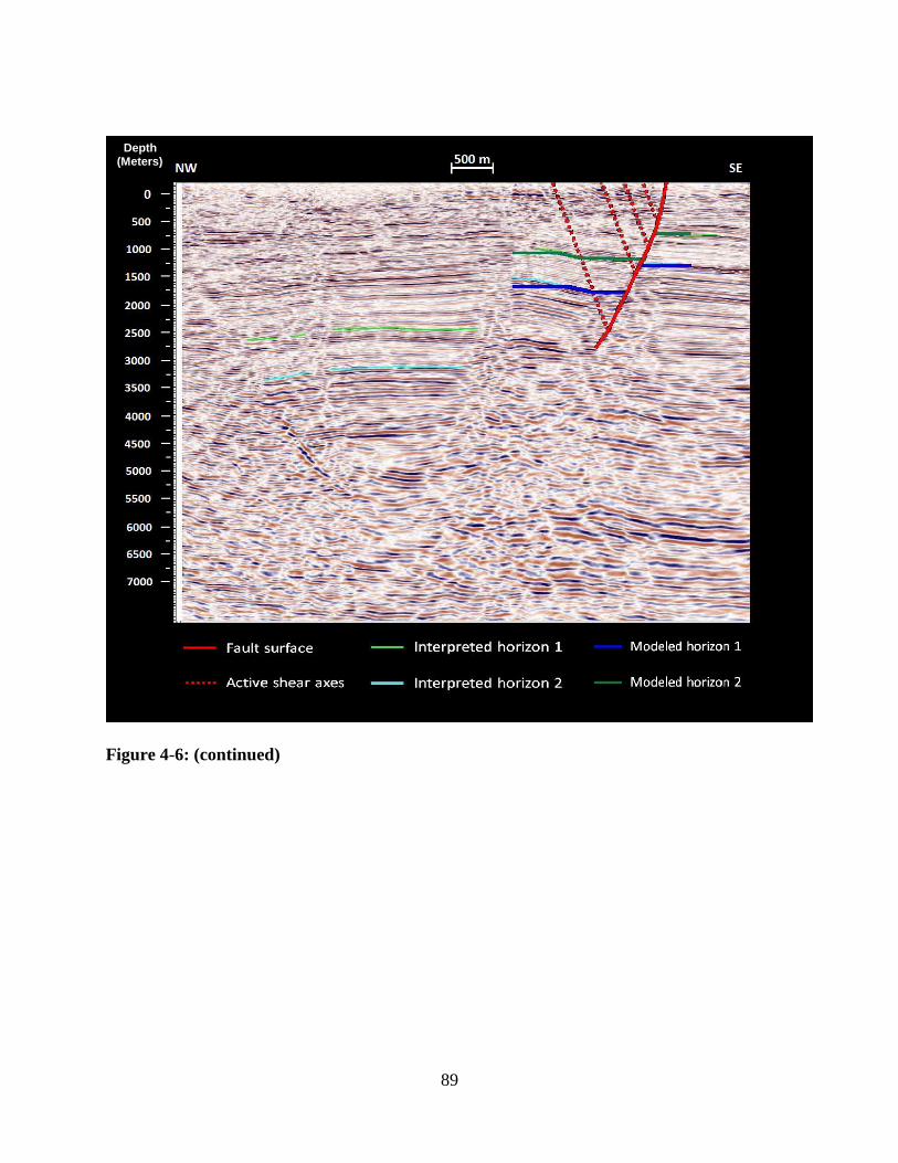
89

Figure 4-6: (continued)

Depth (Meters)

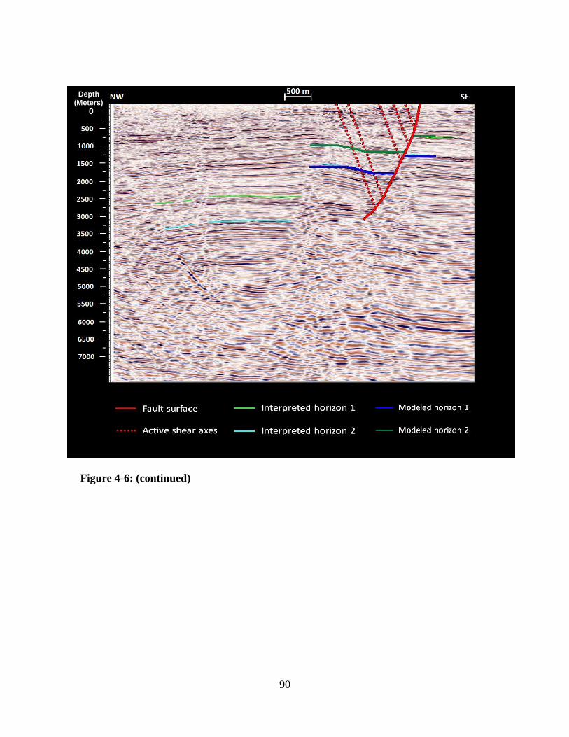
90

Figure 4-6: (continued)

Depth (Meters)

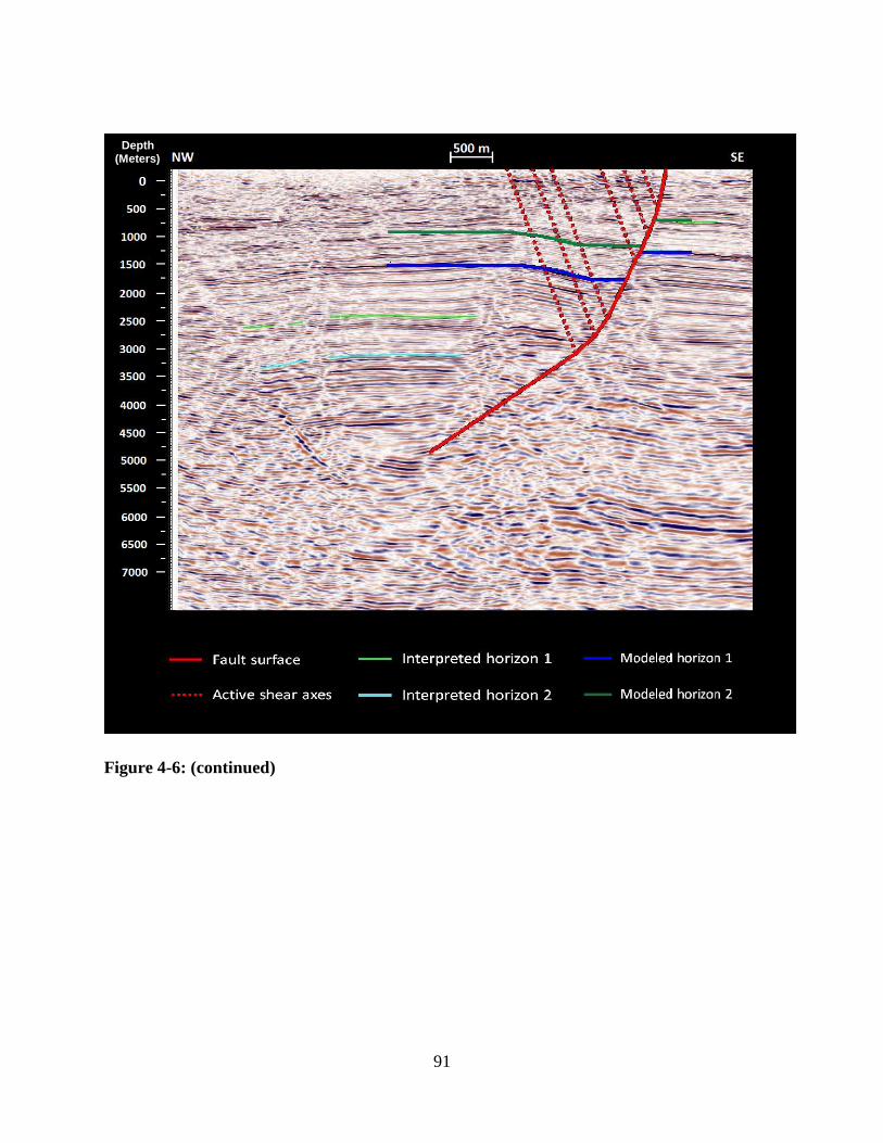
91

Figure 4-6: (continued)

Depth (Meters)

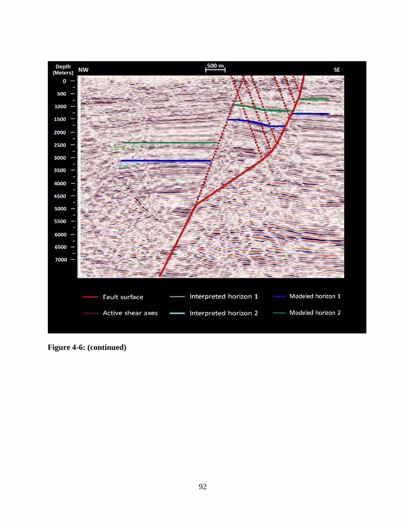
92

Figure 4-6: (continued)

Depth (Meters)

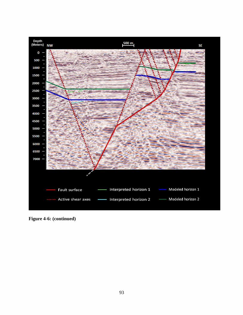
93

Figure 4-6: (continued)

Depth (Meters)

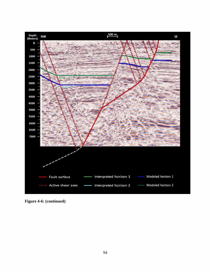
94

Figure 4-6: (continued)

Depth (Meters)

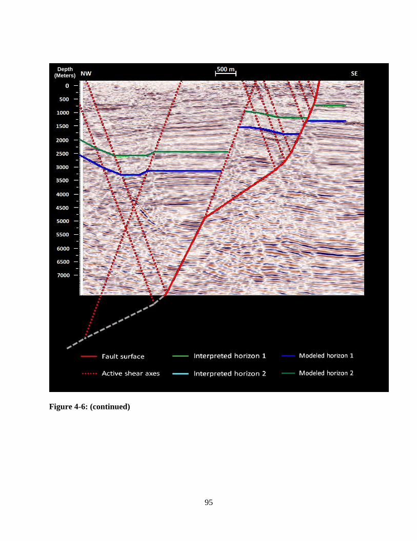
95

Figure 4-6: (continued)

Depth (Meters)

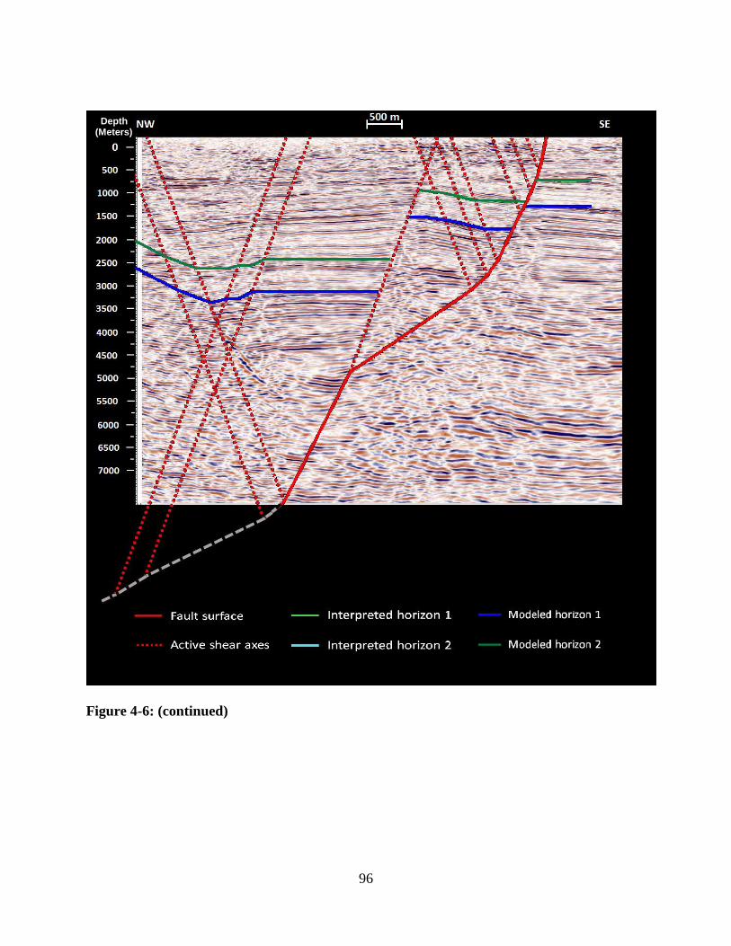
96

Figure 4-6: (continued)

Depth (Meters)

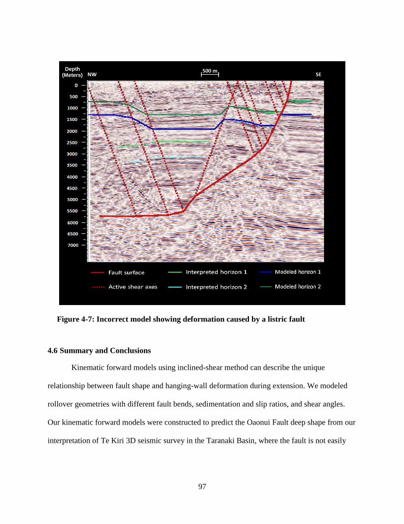
97

Figure 4-7: Incorrect model showing deformation caused by a listric fault

4.6 Summary and Conclusions

Kinematic forward models using inclined-shear method can describe the unique

relationship between fault shape and hanging-wall deformation during extension. We modeled

rollover geometries with different fault bends, sedimentation and slip ratios, and shear angles.

Our kinematic forward models were constructed to predict the Oaonui Fault deep shape from our

interpretation of Te Kiri 3D seismic survey in the Taranaki Basin, where the fault is not easily

Depth (Meters)

98

interpretable at depth. The model suggests that the structure of the Oaonui Fault is a ramp-and-

flat geometry which cuts through the basement at depth of about 6 km (about 3.3 seconds TWT).

99

Conclusions

In this thesis, a major fault that is considered to be active in Taranaki Peninsula was

studied from a 3D seismic reflection volume. Seismic images from the 3D volume reveal the

complex subsurface structure which relates to the tectonic activities and deformation history in

the region since the mid-Cretaceous. North- to north-east trending faults are clearly imaged by

the shallow reflections in the volume. The resolution and quality of the seismic images

deteriorate with depth where faults geometries are not clearly visible.

This thesis also addresses observations of amplitude anomalies and incoherent reflections

within vertical zones along normal faults. The anomalies observed in the seismic images are

likely to be the result of gas migrating upsequence along permeable normal faults. This

conclusion is supported be similar observations of gas leakage in nearby gas fields in the basin.

Seismic attribute analysis can detect the gas presence and delineate the gas distribution in the

survey. Knowledge of geologic history of the region along with the lack of flower structures in

the interpreted seismic volume indicate that deformations associated with faults are mainly due

to dip-slip rather than strike-slip movements. Therefore, the loss of seismic image across faults’

cutoffs, is the result of gas presence rather than distributed strain caused by strike-slip

movement.

In order to evaluate the gas presence and its origin along faults, it is necessary to

understand the geometry of faults at depth and whether they are in contact with the proven

reservoir in the region. In this thesis, the geometry of the major fault in the seismic volume was

modeled using kinematic forward models that are based on the inclined-shear method. The

models predicted the fault’s deep shape based on the shape of deformation in the fault’s hanging

100

wall. This thesis concludes, based on the constructed models, that the major fault in the survey is

a ramp-and-flat geometry which cuts through the basement at about 6 km depth.

101

References

Al-Dossary, S. and K. J. Marfurt, 2006, 3D volumetric multispectral estimates of reflector

curvature and rotation: Geophysics, 71, P41–51.

Alshuhail, A. A., Lawton, D. C., and Chabot, L., 2008, Pembina Cardium CO2 monitoring

project: timelapse seismic analysis: CREWES Research Report, 20.

Anderson, A. L., and L. D. Hampton, 1980a, Acoustics of gas-bearing sediments: 1.

Background: Journal of the Acoustical Society of America, 67, 1865–1889.

Bjørkum, P. A., Walderhaug, O. and Nadeau, P. H., 1998, Physical constraints on hydrocarbon

leakage and trapping revisited: EAGE Petroleum Geoscience, 4, 237-239.

Brown, A. R., 2011, Interpretation of Three-Dimension Seismic Data: The American Association

of Petroleum Geologists and the Society of Exploration Geophysicists.

Chopra, S., and Marfurt, K. J., 2007, Seismic attributes for prospect identification and reservoir

characterization: Society of Exploration Geophysicists, Tulsa, OK.

Cloos, E., 1968, Experimental analysis of Gulf Coast fracture patterns: AAPG Bulletin, v. 52,

420-444.

Gibbs, A. D., 1983, Balanced cross-section construction from seismic sections in areas of

extensional tectonics: Journal of Structural Geology, v. 5, p. 1-39.

Davis, G. H., Reynolds, S. J., and Charles F. K., 2012, Structural Geology of Rocks and Regions:

John Wiley & Sons, Inc., Hoboken, NJ.

102

Dissen, V. R., Barrell, D., Litchfield, N., Villamor, P., Quigley, M., King, A., Furlong, K., Begg,

J., Townsend, D., Mackenzie, H., Stahl, T., Noble, D., Duffy, B., Bilderback, E., Claridge, J.,

Klahn, A., Jongens, R., Cox, S., Langridge, R., Ries, W., Dhakal, R., Smith, A., Horblow, S.,

Nicol, R., Pedley, K., Henham, H., Hunter, R., Zajac, A., Mote, T., 2011, Surface rupture

displacement on the Greendale Fault during the Mw 7.1 Darfield (Canterbury) earthquake,

New Zealand, and its impact on man-made structures, Auckland, New Zealand: Ninth Pacific

Conference on Earthquake Engineering: Building an Earthquake-Resilient Society, 14-16 Apr

2011.

Dula Jr, W. F., 1991, Geometric Models of Listric Normal Faults and Rollover Folds (1); AAPG

Bulletin, 75(10), 1609-1625.

Fossen, H., 2010, Structural geology: Cambridge University Press, Cambridge, U.K.

Gibbs, A. D., 1983, Balanced cross-section construction from seismic sections in areas of

extensional tectonics: Journal of Structural Geology, v. 5, p. 1-39.

Hale, D., 2013, Methods to compute fault images, extract fault surfaces, and estimate fault

throws from 3D seismic images: Geophysics, v. 78, No. 2, O33-O43.

Herron, D. A., 2011, First steps in seismic interpretation: Geophysical monograph series, no. 16.

Herron, D. A., 2000, Pitfalls in seismic interpretation: Depth migration artifacts: The Leading

Edge, v. 19, No. 9, 1016-1017.

Løseth, H., M. Gading, and L. Wensaas, 2009, Hydrocarbon leakage interpreted on seismic data:

Marine and Petroleum Geology, v. 26, no. 7, 1304–1319.

King, P.R. 1991. Physiographic maps of the Taranaki Basin - Late Cretaceous to Recent. New

Zealand Geological Survey Report G155.

103

King, P.R., Naish, T.R., Thrasher, G.P. 1991. Structural cross sections and selected palinspastic

reconstructions of the Taranaki Basin, New Zealand. New Zealand Geological Survey report

G150.

King, P. R., and Thrasher, G. P., 1996, Cretaceous Cenozoic geology and petroleum systems of

the Taranaki Basin, New Zealand (Vol. 2). Institute of Geological & Nuclear Sciences.

Lindsey, J. P., 1989, The Fresnel zone and its interpretive significance: The Leading Edge, 10,

33–39.

Lawton, D. C., Bertram, M. B., Hall, K. W., Bertram, K. L., and Pettinga, J., 2013, Imaging

Unknown Faults in Christchurch, New Zealand, after a M6. 2 Earthquake. In 75th EAGE

Conference & Exhibition incorporating SPE EUROPEC 2013.

Lawton, D. C., Bertram M. B., Margrave, G. F. and Gallant, E. V., 2006, Comparisons between

data recorded by several 3-component coil geophones and a MEMS sensor at the Violet

Grove monitor seismic survey: CREWES Research Report, 18.

Lines, L. R., and Newrick, R. T., 2004, Fundamentals of geophysical interpretation: Society of

Exploration Geophysicists, Tulsa, OK.

Marfurt, K., R. Kirlin, S. Farmer, and M. Bahorich, 1998, 3-D seismic attributes using a

semblance-based coherency algorithm: Geophysics, 63, 1150–1165.

Mavko, G., Mukerji, T., and Dvorkin, J., 2003, The Rock Physics Handbook, 51 p. Cambridge

University Press, Cambridge, U.K.

104

McClay, K. R., & Ellis, P. G., 1987, Geometries of extensional fault systems developed in model

experiments; Geology, 15(4), 341-344.

Meldahl, P., R. Heggland, B. Bril, and P. de Groot, 2001, Identifying faults and gas chimneys

using multiattributes and neural networks: Leading Edge, v. 20, no. 5, p. 474–482

Mouslopoulou, V., Nicol, A., Walsh, J. J., Begg, J. G., Townsend, D. B., & Hristopulos, D. T. ,

2012, Fault-slip accumulation in an active rift over thousands to millions of years and the

importance of paleoearthquake sampling: Journal of Structural Geology, 36, 71-80.

Nodder, S. D., 1993, Neotectonics of the offshore Cape Egmont fault zone, Taranaki basin, New

Zealand: New Zealand Journal of Geology and Geophysics, 36(2), 167-184.

Nunns, A. G., 1991, Structural Restoration of Seismic and Geologic Sections in Extensional

Regimes (1); AAPG Bulletin, 75(2), 278-297.

NZP&M, 2013, New Zealand Petroleum Basins: New Zealand Petroleum & Minerals.

Sheriff, R., 1980, Nomogram for Fresnel zone calculation: Geophysics, 45, 968– 972.

Sheriff, R. E., 2002, Encyclopedic dictionary of exploration geophysics, 4th ed.: SEG

Geophysical Reference Series no. 1.

Suggate, R.P., Stevens, G.R., Te Punga, M.T. (eds), 1978, The geology of New Zealand:New

Zealand Geological Survey, Department of Scientific and Industrial Research, Wellington.

Thrasher, G. P., 1990b, Tectonics of the Taranaki Rift. In 1989 New Zealand Oil Exploration

Conference proceedings: 124–133. Ministry of Commerce, Wellington.

105

Thrasher, G.P. 1990b. Tectonics of the Taranaki Rift. In 1989 New Zealand Oil Exploration

Conference proceedings: 124–133. Ministry of Commerce, Wellington.

Townsend, D., Nicol, A., Mouslopoulou, V., Begg, J. G., Beetham, R. D., Clark, D., ... & Walsh,

J. J. (2010). Palaeoearthquake histories across a normal fault system in the southwest

Taranaki Peninsula, New Zealand. New Zealand Journal of Geology and Geophysics, 53(4),

375-394.

Quigley, M., P. Villamor, K. Furlong, J. Beavan, R. Van Dissen, N. Litchfield, T. Stahl, B.

Duffy, E. Bilderback, D. Noble, D. Barrell, R. Jongens, and S. Cox, 2010, Previously

unknown fault shakes New Zealand's South Island: EOS Transactions, AGU, 91, 469–471.

Shaw, J. H., Hook, S. C., & Sitohang, E. P., 1997, Extensional fault-bend folding and synrift

deposition: An example from the Central Sumatra Basin; Indonesia. AAPG bulletin, 81, 367-

379.

Spang, J. H., & Dorobek, S. L., 1998, Using Antithetic Normal Faults to Map Growth Axial

Surfaces.

Taner, M. T. , 2001, Seismic Attributes: CSEG Recorder, 48-56.

Taner, M. T., 2002, System for estimating the locations of shaley subsurface formations., U.S.

Patent No. 6,487,502. 2

Voggenreiter, W.R. 1993. Structure and evolution of the Kapuni Anticline, Taranaki Basin, New

Zealand: evidence from the Kapuni 3D seismic survey. New Zealand journal of geology and

geophysics 36: 77–94.

White, N. J., Jackson, J. A., and Mckenzie, D. P., 1986, The relationship between the geometry

of normal faults and that of the sedmentary layers in their hanging walls: Journal of Structure

106

Geology, 8(8), 897-909.

Widess, M. B., 1973, How thin is a thin bed?: Geophysics, 38(6), 1176-1180.

Xiao, H., & Suppe, J., 1992, Origin of Rollover (1): AAPG Bulletin, 76(4), 509-529.

Yilmaz, Öz, 2001, Seismic data analysis: Society of Exploration Geophysicists, Tulsa.