A Comprehensive Test of Order Choice Theory: Recent Evidence from the NYSE

Andrew Ellul

Indiana University

Craig W. Holden Indiana University

Pankaj Jain

University of Memphis

Robert Jennings Indiana University

November 10, 2003

Abstract: We perform a comprehensive test of order choice theory from a sample period when the NYSE trades in decimals and allows automatic executions. We analyze the decision to submit or cancel an order or to take no action. For submitted orders we distinguish order type (market vs. limit), order side (buy vs. sell), execution method (floor vs. automatic), and order pricing aggressiveness. We use a multinomial logit specification and a new statistical test. We find a negative autocorrelation in changes in order flow exists over five-minute intervals supporting dynamic limit order book theory, despite a positive first-order autocorrelation in order type. Orders routed to the NYSE’s floor are sensitive to market conditions (e.g., spread, depth, volume, volatility, market and individual-stock returns, and private information), but those using the automatic execution system (Direct+) are insensitive to market conditions. When the quoted depth is large, traders are more likely to “jump the queue” by submitting limit orders with limit prices bettering existing quotes. Aggressively-priced limit orders are more likely late in the trading day providing evidence in support of prior experimental results. JEL Classification Code: G10 Keywords: Order choice, limit order, market order, automatic execution, limit order book Addresses for correspondence: Andrew Ellul (anellul@indiana.edu), Craig Holden (cholden@ indiana.edu) and Robert Jennings (jennings@indiana.edu) are from the Kelley School of Business, Indiana University, 1309 E. Tenth St., Bloomington, IN 47405-1701. Pankaj Jain (pjain@memphis.edu) is from the Fogelman College of Business, University of Memphis, Memphis, TN 38152. Acknowledgements: We thank Morgan Stanley & Co., Inc. for financial support and the New York Stock Exchange for providing data. The opinions expressed in this paper do not necessarily reflect those of the employees, members, or directors of the New York Stock Exchange, Inc. We thank Robert Battalio, Joel Hasbrouck, Christine Parlour and seminar participants at Indiana University, the National Bureau of Economic Research Market Microstructure Workshop, the New York Stock Exchange, the Ohio State University, Pennsylvania State University, and Vanderbilt University for useful comments. We are responsible for any errors.

1

A Comprehensive Test of Order Choice Theory: Recent Evidence from the NYSE

A large theoretical literature on market microstructure develops the trader’s optimal order

choice under a wide variety of trading mechanisms and market conditions. For example, Parlour

(1998) finds that when an order depletes the depth available on a limit order book, the next trader

is likely to choose an order replenishing depth (i.e., a market buy order is more likely followed

by a limit sell). Thus, she predicts what can be thought of as negative autocorrelation in order

type. Handa and Schwartz (1996) model the time that different investors allow themselves to

trade and find that impatient traders endogenously choose market orders, whereas patient traders

endogenously choose limit orders. By (informal) extension, we posit that extremely impatient

traders might choose immediate automatic execution over slower floor execution and that their

orders might be submitted virtually irrespective of how favorable or unfavorable the market

conditions. Other variables predicted to effect order choice include quoted spread (Cohen, Maier,

Schwartz, and Whitcomb 1981; Harris 1998; and Foucault 1999), volatility (Foucault 1999),

prior own and market return (Brown and Jennings 1990), and time of day (Harris 1998;

Hollifield, Miller, and Sandås 1999; Bloomfield, O’Hara, and Saar 2002).

We provide a comprehensive test of order choice theory. This tests some theories that

have not been tested and tests many theories simultaneously. We use NYSE system order data to

estimate a multinomial logit model of order choice. We study a wide spectrum of order choices

including order type (market vs. limit), order side (buy vs. sell), order pricing aggressiveness

(executable vs. limit prices better than, equal to, or worse than the current quote), order

cancellation, execution method (automatic vs. floor), and the fundamental choice of doing

nothing vs. order activity. Our multivariate analysis includes 17 independent variables designed

to test theoretical order-choice models. We analyze a several sub-samples and conduct

2

robustness checks. Thus, we obtain a comprehensive and robust set of conclusions about how

well actual NYSE order choices conform to what is predicted by theory.

We also provide the first analysis of order choice on the New York Stock Exchange

(NYSE) from the era of decimal prices (i.e., penny tick size) and automatic executions via the

NYSE’s Direct+ system. Recent studies document how profound both of these changes are.

Chakravarty, Harris, and Wood (2001) find that switching to decimal prices yields more frequent

and smaller quote adjustments, smaller quoted and effective spreads, and smaller depths. In

addition, Bacidore, Battalio, and Jennings (2003) find that decimal prices result in a roughly 50%

reduction in cumulative depth on the limit order book, smaller order sizes, and more frequent

cancellations. Jain (2002) analyzes 118 exchanges around the world and documents that the

switch from a pure floor-based system to a combined floor and electronic system results in a

lower cost of capital, higher volatility, and more volume. These market structure changes are

very likely to impact order choice. Therefore, we believe it is interesting to analyze order choice

on the NYSE from the decimal, Direct+ era. This complements prior work on order choice that

analyzes the Paris Bourse (Biais, Hillion, and Spatt 1995), NASDAQ (Smith 2000), or 1990-

1991 NYSE using the TORQ dataset (Baewho, Jang, and Park 2002; Beber and Caglio 2002).

Order choice is important because it is the foundation of how the NYSE (or any security

market) operates. Order submission and cancellation choices are central to the supply of and

demand for liquidity. NYSE liquidity is provided by specialists and floor brokers, but public

limit orders play a major role. For example, Kavajecz (1999) finds that public limit orders are

represented in 64% of NYSE specialists’ quotes. Recent NYSE initiatives, such as Direct+ and

OpenBook, have increased public limit orders’ importance. If we can better understand the

market conditions under which traders demand liquidity and those under which (and at what

3

prices) they supply liquidity, then we can better understand the price formation process –

markets’ most important role. In addition, order choice affects execution quality, which is

important to both consumers and regulators (for example, see SEC 2001b).

One of our findings relates to Biais, Hillion, and Spatt (1995), who use descriptive

statistics to demonstrate that the Paris Bourse exhibits positive first-order, serial correlation in

order type (i.e., a limit sell order is most likely to be followed by another limit sell). This finding

is counter to Parlour’s theoretical prediction and rather puzzling because it suggests that the limit

order book grows more and more imbalanced. We find that the NYSE also exhibits positive

first-order, order-type serial correlation in 2001. This is true in a multivariate setting where we

control for other influences and is quite robust. Biais, Hillon, and Spatt suggest that this result

might be an artifact of order-splitting (i.e., a large limit sell is split into a sequence of smaller

limit sells). Our dataset identifies the firm and the specific branch within the firm submitting the

order. This allows us to identify orders that appear to be split. We adjust the order flow process

for order splitting, but still obtain positive first-order, serial correlation in order type. However,

when we look at longer time horizons (five minute intervals), we find negative serial correlation

in changes in the order flow processes. The positive order-to-order serial correlation and

negative five-minute serial correlation in changes can be reconciled. Both results are consistent

with an order flow process that has inertia order-by-order, but slowly mean-reverts. Our finding

of a slow mean-reverting order flow process resolves the puzzle of why the limit order book does

not continue to become more imbalanced and supports Parlour’s theoretical predictions.

Another key finding is that orders sent to Direct+ for automatic execution are much less

sensitive to market conditions than orders sent to the floor. In other words, Direct+ orders are

submitted with little respect for the previous order type, the current quoted spread or depth,

4

recent volume or volatility, past own or market return, or time of day. This is consistent with the

claim that extremely impatient traders choose fast automatic execution no matter what; whereas

only moderately impatient traders send their marketable orders to the floor with economically

meaningful regard for market conditions.

We have several additional findings. We document that, when the quoted depth is large,

traders are more likely to “jump the queue” by submitting limit orders with limit prices bettering

existing quotes and less likely to submit orders with limit prices equal to or worse than current

quotes. In addition, a favorable (unfavorable) forecast of the rest-of-the-day stock return, as

proxied by the realized rest-of-the-day stock return, increases the likelihood of a buy (sell) order.

This provides evidence that some traders appear to be effectively exploit private information. If

the recent market return is positive (negative), then more buy (sell) orders arrive. This is

consistent with momentum-oriented technical trading. We find that order activity is clustered.

We find that doing nothing, defined as time passing with-out order activity, also is clustered.

Consistent with previous work, we find that wider (narrower) spreads increase the probability

of market (limit) orders. However, we find that effect is limited primarily to small orders.

Finally, we find that limit orders are more likely late in the trading day, which is inconsistent

with the Harris (1998) and Hollifield, Miller, and Sandås (1999) prediction that traders switch

from market orders to limit orders late in the trading day. The fact that this result is driven

mostly by aggressively-priced orders is consistent with Bloomfield, O’Hara, and Saar (2002)

who provide experimental evidence that informed traders switch from demanding liquidity early

in the day to provide liquidity late in the day.

To assess the economic significance of an explanatory variable’s impact on order choice,

we calculate what we refer to as an impulse sensitivity. An impulse sensitivity is the change in

5

the estimated probability of the dependent variable caused by a one standard deviation shock in

the explanatory variable. To determine the statistical significance of the direction of change in

the estimated probability, we test the statistical significance of the impulse sensitivities, not the

statistical significance of the multinomial logit coefficients. To the best of our knowledge, there

is no technique in the prior literature to perform such a test, so we develop a test of the statistical

significance of the impulse sensitivity.

The paper is organized as follows. Section 1 presents a literature review and states our

hypotheses. Section 2 describes the data we obtain from the NYSE. In Section 3, we explain the

empirical methodology. Section 4 presents our results. Section 5 concludes. The appendix

describes our new test of the statistical significance of an impulse sensitivity.

1. Literature Review and Hypotheses

Last Event. Parlour (1998) develops a model of a transparent limit order book with

symmetric information. The probability of executing a limit order depends on the book’s state

and the trader’s patience. Parlour notes that the arrival of a limit buy (sell) order lengthens the

queue at the bid (ask) side of the book. This reduces the attractiveness of submitting another

limit order of the same kind. Hence, we should observe negative serial correlation in order type.

Last Event Hypothesis: The probability of observing a limit buy (sell) is lowest if the

immediately preceding event is a limit buy (sell).1

Last Five Minutes. In contrast with Parlour’s assumption of full transparency, the NYSE

limit order book was closed to off-exchange traders during our sample period. In other words,

off-exchange traders might not see the last order before making their order choice. Although

marketable orders usually fill and print quickly, specialists have 30 seconds to post limit orders

with prices equaling or bettering current quotes and limit orders with limit prices worse than the 1 All hypotheses are stated as the alternative.

6

contemporaneous quotes are completely non-transparent to off-floor traders. To give the Parlour

model a better chance to predict NYSE order strategy, we aggregate each type of order flow in

five-minute intervals and test for serial correlation in changes in the order flow process. The

aggregation of order flow in the prior five-minute interval might better represent what a trader

not on the floor of the NYSE can consider when submitting an order.2

Last Five Minutes Hypothesis: The change in the number of limit buys (sells) over five-

minute intervals is lower if the change in the number of limit buys (sells) over the preceding

five-minute interval is higher.

Auto-ex vs. Floor. In 2000 the NYSE introduced Direct+; an electronic system that

automatically executes small, marketable buy (sell) orders at the quoted ask (bid) price. The size

of a Direct+ order is limited to the size of the quote it is trying to hit or 1099 shares, whichever is

less. These orders fill within 2 or 3 seconds of arriving at the Exchange and are not eligible for

price improvement. By contrast, marketable orders routed to the floor typically take 20 to 40

seconds to execute and often receive price improvement from the floor’s oral auction process.

Informally extending the Handa and Schwartz (1996) model, contrast an extremely

impatient trader who believes he must trade in only a few seconds to a moderately impatient

trader whose believes she must trade within the next one minute. The extremely impatient trader

might endogenously choose automatic execution and his order might be submitted with little

regard for market conditions. The moderately impatient trader might choose floor execution to

get a better price on average and her order might have more regard for market conditions.

Auto-ex Hypothesis: The sensitivity of automatically executed orders to market

conditions is less than the sensitivity of floor orders to market conditions.

2 Obviously, there are limitations to how closely the NYSE resembles the theoretical market modeled by Parlour, which limits our ability to test her model precisely.

7

Spread. Harris (1998) finds that wider spreads increase the cost of demanding liquidity

and increase the reward to providing liquidity. This causes the marginal investor to switch from

taking liquidity via market orders to supplying it with limits. Alternatively, Foucault (1999) finds

that an increase in market volatility makes liquidity demanders less patient, which allows limit

order submitters to widen their spread in order to extract greater rents. So, there is a positive

relation between spreads and limit orders and a negative relation between spreads and market

orders. Biais, Hillion and Spatt (1995), Harris (1998), Hollifield, Miller and Sandås (1999),

Smith (2000), Bae, Jang and Park (2002), and Ranaldo (2002) find evidence consistent with this

claim. We extend the literature in two ways. First, we test the spread hypothesis differentiating

between marketable limit orders and non-marketable limit orders. Second, we test the spread

hypothesis differentiating between small, medium, and large orders.

Spread Hypothesis: Narrow (wide) spreads increase the probability of marketable (non-

marketable) orders.

Depth. Berber and Caglio (2002) and Ranaldo (2000) analyze the quoted depth’s effect

on order submission decisions. We extend the literature by investigating whether both sides of

the quote seem to affect order choice or if only one side of the quote appears to matter to traders.

We also test whether large ask (bid) depth appears to be viewed as forecasting a short-term price

decrease (increase), leading to more sells (buys). Finally we test whether a larger ask (bid) depth

makes it more attractive to “jump-the-queue” by submitting a limit sell (buy) order with a limit

price better than the quote and conversely less attractive to submit a limit sell (buy) order with a

limit price equal to or worse than the quote.

Short-term Forecasting Hypothesis: Large ask (bid) depth increases the probability

of both a limit sell (buy) and a market sell (buy).

8

Jump-The-Queue Hypothesis: Large ask (bid) depth increases the probability of an

inside-the-quote limit sell (buy) and decreases the probability of an at-the-quote or behind-the-

quote limit sell (buy).

Volatility. Foucault (1999) suggests a model of a dynamic limit order market where

across-agent variation in the consensus belief about asset valuation leads to a winner’s curse

problem for traders. With greater volatility, limit orders are placed at less competitive prices as a

compensation for the adverse selection risk. Volatility also makes market orders less profitable.

In equilibrium, the proportion of limit orders increases when return volatility is high. Although

Foucault examines the cross-section of securities, his prediction might be extended to the time-

series realm if traders can predict volatility (say, via a GARCH model). Handa and Schwartz

(1996) also predict that investors submit more limit orders when volatility rises. Smith (2000),

Ahn, Bae, and Chan (2001), Danielsson and Payne (2002), Hollifield, Miller, Sandås and Slive

(2002), and Ranaldo (2002) find evidence consistent with a direct relation between security price

volatility and limit order arrival frequency. Hasbrouck and Saar (2002), however, find the

opposite. In addition, increased volatility in the stock price might be a result of the arrival of

valuation-relevant information. If this is the case, then we anticipate that no trading activity is

less likely immediately following volatile periods.

Volatility Hypothesis: Higher return volatility is associated with more frequent limit

orders and less frequent periods of no trading activity.

Market Return and Own Return. Technical traders use public information reflected in

security prices (such as own returns, market returns, etc.) to forecast future price movements. An

extensive academic literature analyzes technical trading rules based on past security/market

returns (see Brown and Jennings 1990; Gencay 1998; Sullivan 1999; Lo, Mamaysky, and Wang

9

2000; Ready 2002). It is not unusual for day traders to use minute-by-minute “momentum” or

“contrarian” trading strategies.3 The presence of such traders suggests that there may be short-

term patterns to exploit. We allow for this possibility with the following hypothesis.

Market Return Hypothesis: A non-zero market return is associated with changes in

order choice.

Own Return Hypothesis: A non-zero own return is associated with changes in order

choice.

Time-of- day. In addition to the well-documented U-shaped intra-day pattern in trading

activity (e.g. Chung, Van Ness and Van Ness 1999), the economics literature notes a “deadline

effect,” where agreements are more likely to be reached at the last minute. For example, Roth et

al (1988) conduct experiments testing for bargaining patterns through time and find that many

agreements occur just before the deadline. This suggests that traders become more aggressive as

the close of trading approaches. In contrast, Bloomfield, O’Hara and Saar (2002) use an

experimental asset market to model traders’ behavior in an electronic limit order book. They

find that liquidity provision evolves during the trading day. Informed traders demand liquidity

early in the trading session by submitting orders that hit existing limit orders but become

suppliers of liquidity by submitting more limit orders towards the end of the trading day.

Time of Day Hypothesis: As the close of the trading day approaches, the distribution of

order types changes.

We simultaneously test these hypotheses using a multinomial logit model and electronic order

data from the New York Stock Exchange.

3 See many examples in “Risky Business: The Day Traders” in the Investigate Reports video series available on the A&E web site (www.aetv.com).

10

2. Data

We obtain system order data from the NYSE. Because of the volume of data, we select a

sample of NYSE-listed equity securities. Initially, we choose the 50 most actively traded NYSE

stocks during the 20 trading days prior to January 29, 2001. We also randomly select 25 stocks

from each of four Volume-Price groups. To pick the 100-stock random sample, we rank NYSE-

listed securities on share trading volume and, separately, on average NYSE trade price during the

20 trading days prior to January 29, 2001. Each security is placed into one of four categories

after comparing its share price to median NYSE share price and its trading volume to median

NYSE volume. These groups (of unequal numbers of stocks) are a high-volume:high-price

group, a high-volume:low-price group, a low-volume:high-price group, and, a low-volume:low-

price group. Within each group, we arrange securities alphabetically (by symbol) and choose

every Nth security, where N is chosen to select 25 securities from that group. Because two of the

50 stocks with the highest trading volume also are randomly chosen as part of the high volume

groups, our final sample has 148 securities.

We use the NYSE’s System Order Database (SOD) and its companion quote file (SODQ)

to provide an audit trail of system (SuperDOT) orders arriving during the week of April, 30 to

May 4, 2001.4 SOD contains order and execution information for NYSE system orders. Order

data include security, order type, a buy-sell indicator, order size, order date and time, limit price

(if applicable), and the identity of the member firm submitting the order. Execution data include

the trade’s date and time, the execution price, the number of shares executing, and (if relevant)

cancellation information. SODQ contains the NYSE quote and the best non-NYSE quote at the

time an order arrives and at trade time. All records (orders, executions, and cancellations) are

4 We have data for April, May, and June for the 148 sample stocks. The large number of order submissions and cancellations makes sampling necessary. We choose this week for our sample period because it appears “typical” of the entire time period in terms of market return and order mix.

11

time-stamped to the second. System orders represent about 93% of reported NYSE orders and

47% of reported NYSE share volume.5 Specifically, these data do not include most of the orders

routed to the specialists’ trading posts via floor brokers. Thus, we study only a subset of NYSE

order choices; those resulting in electronic submission of orders. Generally, these are the

smaller, more easily executed orders. Our sample includes over 5.1 million events. We exclude

orders arriving when the National Best Bid (NBB) price exceeds the National Best Offer (NBO)

price or when the NBB or NBO size is zero.6

Table 1 provides some descriptive statistics for these and other variables.

[Insert Table 1.]

The mean order size is 1,232 shares. Although this is relatively small, we have large orders, as

suggested by the maximum order size of 900,000 shares. On average, our sample stocks have

2.24 million shares trading per day, which is a .106% turnover rate. This undoubtedly exceeds

the typical NYSE stock because our sample includes the 50 most actively traded NYSE stocks.

The average NYSE bid (offer) depth is 2,760 (3,701) shares. For the sample stocks (again,

oriented to the more actively traded NYSE stocks), the spread averages 0.15% of the stock’s

$43.80 average “price,” i.e., bid-ask spread midpoint. We do, however, have some observations

where the spread is a large fraction of the stock’s price. The average time of an event is 153.76

five-minute intervals past midnight, or approximately 12:48pm. The average five-minute own-

and market-return are positive during the sample period. The own-return has more cross-

sectional volatility than the market return. The private information variable (measured as the

change in the quote midpoint between order arrival time and that day’s closing) averages 0.27%.

5 See SEC (2001a), page 5. 6 The National Best Bid (Offer) price is the higher (lower) of the NYSE bid (ask) and the best non-NYSE bid (ask).

12

3. Methodology

3.1. Variables

We analyze the likelihood of observing particular events – the submission of different

order types and order cancellations. In addition, because the trader can choose to do nothing, we

design a role for clock time passing with no activity. Specifically, we define a no-activity event

as a stock-specific time interval passing without an order submission or cancellation. The no-

activity time interval is defined as either: (1) the median time between successive order events,

or (2) five minutes, whichever is less. There is considerable variation across stocks in their no-

activity time intervals. The eight most active stocks have a no-activity time interval of one

second. The 50 least active stocks have a median time between events exceeding five minutes

and, thus, receive a no-activity time interval of five minutes. Easley, Kiefer, and O’Hara (1997)

use a similar no-activity event to model and estimate the passage of clock time without activity.

Beginning with the first trade of each day, we compute the time between successive pairs

of order submissions/cancellations. If the elapsed time exceeds the no-activity interval, then we

insert the appropriate number of no-activity events. For example, suppose that a stock has a

median time between order activity events of 20 seconds and that orders arrive at 9:30:00,

9:30:05, and 9:30:50. There are fewer than 20 seconds between the first and second order, so a

no-activity event is NOT inserted. Between the second and third order, we insert no-activity

events at 9:30:25 and 9:30:45. The 4:00:00 closing is taken as the end of the trading day.

We distinguish four order types: Market Buy, Market Sell, Limit Buy and Limit Sell. We

see in Table 1 that these order types account for 57% of the events (= .1250 + .1266 + .1641 +

.1546). Thus, a cancellation or no-activity event occurs 43% of the time. The fact that limit

orders are more frequent than market orders is consistent with extant literature finding that limit

13

orders are more frequent than market orders on the NYSE (e.g., Harris and Hasbrouck, 1996). A

simple count of the dependent variables provides a similar mix of events: no-activity events are

32.5% of the observations, cancellations are 14.8%, limit buy orders are 18.0%, limit sell orders

are 17.1%, and market buys and sells orders are 8.8% each.

Our analysis differentiates among four types of limit orders: behind-the-quote, at-the-

quote, inside-the-quote, and marketable. We place each limit order into one of the categories by

comparing the limit price to NYSE quoted prices. Behind-the-quote buy (sell) orders have limit

prices less (more) than the NYSE bid (ask) price. At-the-quote buy (sell) orders have limit

prices equal to the NYSE bid (ask) price. Inside-the-quote orders have limit prices between the

NYSE bid price and the NYSE ask price. Finally, buy (sell) marketable limit orders have limit

prices greater (less) than or equal to the NYSE ask (bid) price.7 Behind-the quote limit orders

are the least aggressive and market orders are the most aggressive. We distinguish between the

cancellations of buy and sell orders. To identify the model, one event must be designated as the

base case. We arbitrarily designate the no-activity event as our base case.

Based on extant theoretical and empirical work on order submission strategy, we identify

17 explanatory variables.8 We define these variables below.

1. Last event market buy takes the value of 1 if the previous event was a buy market order and 0 otherwise; 2. Last event market sell takes the value of 1 if the previous event was a sell market order and 0 otherwise; 2. Last event limit buy takes the value of 1 if the previous event was a limit buy order and zero otherwise; 4. Last event limit sell takes the value of 1 if the previous event was a limit sell order and zero otherwise;

7 Peterson and Sirri (2002) provide a more detailed discussion of marketable limit orders. 8 Using the Belsley, Kuh, and Welsch (1980) method, we do not find a muti-collinearity problem among our explanatory variables.

14

5. Last event cancel buy takes the value of 1 if previous event was cancellation of a buy order and 0 otherwise; 6. Last event cancel sell takes the value of 1 if the previous event was cancellation of a sell order and 0 otherwise; 7. Percentage spread is measured as the NYSE bid-ask spread divided by the average of the bid and ask prices at the time the order is submitted; 9 8. Relative NYSE Bid size is the size (in hundreds of shares) associated with the NYSE’s bid price at the time of the event divided by the number of shares outstanding (in millions); 9. Relative NYSE Ask size is the size (in hundreds of shares) associated with the NYSE’s ask price at the time of the event divided by the number of shares outstanding (in millions); 10. Relative volume is the natural logarithm of the number of shares traded in the five-minute interval prior to the event divided by the number of shares outstanding; 11. Own return is the percent change in the stock’s midpoint (i.e., the average of the best bid and best ask prices) in the five-minute interval before the event; 12. Own return squared is the stock’s own return squared; 13. Market return is the percentage change in the quoted spread’s midpoint for the exchange traded fund mimicking the S&P500 (SPY) in the five-minute interval prior to the event; 14. Time is the time of day of the event expressed as the number of five-minute intervals since midnight (e.g., 9:30:00am to 9:34:59am is interval 114); 15. Time from noon squared is the deviation of the event’s time interval from the mid-day time interval (153) squared; 16. Private information is a measure of the traders’ current private information as proxied by the future change in stock value. It is calculated as [(closing NYSE quoted spread midpoint) - (order-time NYSE quoted spread midpoint)]/(order-time NYSE quoted spread midpoint); and, 17. NYSE not at the NBBO is a binary variable equal to one in the case that the NYSE bid is not equal to the National Best Bid or in the case that NYSE offer is not equal to the National Best Offer and it’s equal to zero otherwise.

9 We obtain similar results if we use both dollar spread and price (or inverse price) in the regressions.

15

3.2. Models

We specify the following multinomial logit model for each stock i and time t over which

an event can occur.

Event typei,t = a + b1(Last event cancel buy)i,t + b2(Last event cancel sell)i,t + b3(Last event limit

buy)i,t + b4(Last event limit sell)i,t + b5(Last event market buy)i,t + b6(Last event market sell)i,t +

b7(Percentage spread)i,t + b8(Relative NYSE bid size)i,t + b9(Relative NYSE ask size)i,t +

b10(Relative volume)i,t-1 + b11(Own return)i,t-1 + b12(Own return squared)i,t-1 + b13(Market

return)t-1 + b14(Time)t + b15(Time from noon squared)t +b16(Private information)i,t + b17(NYSE

not at NBBO)i,t + ei,t (1)

In this specification, the subscript “t” represents a contemporaneous value. The subscript “t-1”

represents an aggregate value from the preceding five-minute interval. To compute the values

for these five-minute intervals, we begin with the 9:30:00-to-9:34:59 interval. We proceed to

compute values for each five-minute interval throughout the day, ending with the time from

3:55:00 to 4:00:00. Thus, for example, the “t-1” interval associated with an order arriving at

9:42:30 is the 9:35:00-9:39:59 interval. We run two types of multinomial logit models with

different event structures.10

Initially, we analyze a 7-way event structure. The seven events are: (1) cancellation of an

existing buy order, (2) cancellation of an existing sell order, (3) the arrival of a Limit Buy order,

(4) the arrival of a Limit Sell order, (5) the arrival of a Market Buy order, (6) the arrival of a

Market Sell order, or (7) No Activity in a stock-specific time interval since the last event.11 Next,

10 Our approach can be thought of as randomly selecting a single representative trader and assessing his/her actions. We do not model the number of traders present in the market at a particular time. 11 For the 7-way event structure, the “market buy” (“market sell”) event includes marketable limit buys (sells), because both types of orders are liquidity-demanding, executable orders. The “limit buy” (“limit sell”) event

16

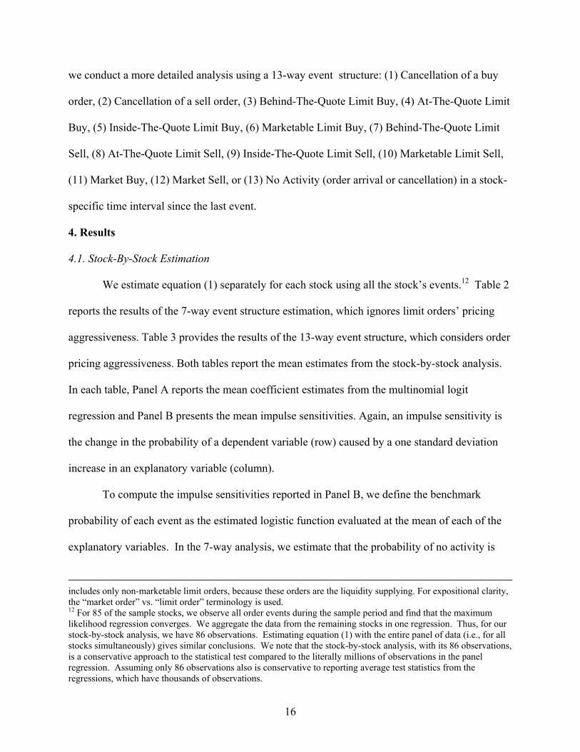
we conduct a more detailed analysis using a 13-way event structure: (1) Cancellation of a buy

order, (2) Cancellation of a sell order, (3) Behind-The-Quote Limit Buy, (4) At-The-Quote Limit

Buy, (5) Inside-The-Quote Limit Buy, (6) Marketable Limit Buy, (7) Behind-The-Quote Limit

Sell, (8) At-The-Quote Limit Sell, (9) Inside-The-Quote Limit Sell, (10) Marketable Limit Sell,

(11) Market Buy, (12) Market Sell, or (13) No Activity (order arrival or cancellation) in a stock-

specific time interval since the last event.

4. Results

4.1. Stock-By-Stock Estimation

We estimate equation (1) separately for each stock using all the stock’s events.12 Table 2

reports the results of the 7-way event structure estimation, which ignores limit orders’ pricing

aggressiveness. Table 3 provides the results of the 13-way event structure, which considers order

pricing aggressiveness. Both tables report the mean estimates from the stock-by-stock analysis.

In each table, Panel A reports the mean coefficient estimates from the multinomial logit

regression and Panel B presents the mean impulse sensitivities. Again, an impulse sensitivity is

the change in the probability of a dependent variable (row) caused by a one standard deviation

increase in an explanatory variable (column).

To compute the impulse sensitivities reported in Panel B, we define the benchmark

probability of each event as the estimated logistic function evaluated at the mean of each of the

explanatory variables. In the 7-way analysis, we estimate that the probability of no activity is

includes only non-marketable limit orders, because these orders are the liquidity supplying. For expositional clarity, the “market order” vs. “limit order” terminology is used. 12 For 85 of the sample stocks, we observe all order events during the sample period and find that the maximum likelihood regression converges. We aggregate the data from the remaining stocks in one regression. Thus, for our stock-by-stock analysis, we have 86 observations. Estimating equation (1) with the entire panel of data (i.e., for all stocks simultaneously) gives similar conclusions. We note that the stock-by-stock analysis, with its 86 observations, is a conservative approach to the statistical test compared to the literally millions of observations in the panel regression. Assuming only 86 observations also is conservative to reporting average test statistics from the regressions, which have thousands of observations.

17

44%, the probability of a limit buy (sell) order of 18% (17%), the probability of a market buy or

market sell order is 9%, and the probability of a cancelled order is 3.65%. The 13-way analysis

provides similar estimates of the likelihood of cancellations and marketable orders, but estimates

that limit orders are less likely (14% for buys and 16% for sells) and no-activity intervals are

more likely (49.7%) than the 7-way event model. To compute the change in the probabilities

(impulse sensitivities), we successively re-evaluate the estimated logistic function after adding a

standard deviation to the mean of one explanatory variable without disturbing the means of the

other explanatory variables. Thus, the column labeled “Percent Spread” in Panel B of Tables 2

and 3 reports the impulse sensitivity based on a one standard deviation increase in the percent

spread holding all other explanatory variables constant at their mean levels.

Our hypotheses are statements about the impulse sensitivities, so we discuss, interpret,

and test the impulse sensitivities, not the coefficient estimates. In most cases, the sign of the

multinomial coefficient estimate is the same as that of the impulse sensitivity, but not always.13

For example, in Table 2 Panel A, the Market Buy coefficient in the Last Limit Sell column is

+0.575, but Panel B’s Market Buy impulse sensitivity in the Last Limit Sell column is -0.12%.

What matters for the multinomial logit coefficients is their relative size. In this case, the Market

Buy coefficient is smaller than the other coefficients in the Last Limit Sell column, so the Market

Buy impulse sensitivity is negative and the other non-base case impulse sensitivities are positive.

Because our hypotheses are concerned with the sign of the impulse sensitivities, we wish

to test if an impulse sensitivity is statistically significantly different from zero. There appears to

be no established procedure to do this. The appendix derives a new econometric procedure for

13 They may differ because the multinomial logit coefficients affect the denominator of a probability calculation, as well as the numerator.

18

testing the statistical significance of an impulse sensitivity. We summarize our hypotheses

regarding the expected signs of the impulse sensitivities in Panel C of Table 2.

[Insert Tables 2 and 3.]

Last event. Based on the theoretical work of Parlour (1998) and the empirical work of

Bias, Hillion, and Spatt (1995), we are interested in the first-order serial correlations of order

types. Consider marketable orders. Examining Table 2, we find that marketable buy (sell) orders

are most likely to follow marketable buy (sell) orders. That is, the largest impulse sensitivity in

the “Last Market Buy” (“Last Market Sell”) column is associated with marketable buy (sell)

orders. This is evidence from the marketable order categories of positive serial correlation in

order type (a positive diagonal effect). This finding is consistent with the findings in Biais,

Hillion, and Spatt (1995) and Yeo (2002) and is inconsistent with the Last Event Hypothesis. A

marketable order takes liquidity from the limit order book and produces a shorter queue for new

limit orders to stand behind. Parlor (1998) suggests that liquidity suppliers are more willing to

join shorter queues. Thus, we expect that marketable orders would be followed by limit orders

replenishing the extinguished liquidity (limit sells following market buys and limit buys after

market sells). In fact, we find that the likelihood of limit orders arriving on the opposite side of

the book from where liquidity was taken increases more after the arrival of a marketable order

than the likelihood of a limit order replacing the taken liquidity.

When the previous event is a limit order, the results are equally clear. For limit buy (sell)

orders, the likelihood of a limit buy (sell) increases the most. The positive serial correlation from

the limit order categories also is inconsistent with the Last Event Hypothesis.14 Parlour’s

14 As a robustness check on the positive serial correlation in order type findings, we check two alternative specifications. First, we estimate the same 7-way event structure but drop the spread, bid depth, and ask depth explanatory variables. Second, we estimate the same 7-way event structure but drop the spread, bid depth, ask depth, volume, and volatility explanatory variables. Our thought was that perhaps these highly transparent (to off-floor

19

predictions do not seem to hold on an order-by-order basis. Table 3 confirms that the arrival of a

limit buy (sell) order increases the likelihood of seeing another non-marketable limit buy (sell)

order for all levels of pricing aggressiveness except (including) marketable orders.

Finally, we examine the changes in probabilities conditional on an order’s cancellation.

Our results are consistent with a trader canceling existing limit orders and submitting new ones.

When a buy (sell) order is cancelled, the most likely subsequent event is the arrival of a new buy

(sell) limit order. Table 3 indicates that the increase in likelihood of non-marketable limit orders

is common across all levels of pricing aggressiveness.

Activity and No Activity. We see that most of the impulse sensitivities associated with the

last event variables are positive. This suggests that order activity is clustered – the arrival or

cancellation of any type of order significantly increases the likelihood of additional order activity

and decreases the likelihood of no activity.

No activity is also clustered. To see this, note that the arrival or cancellation of an order

significantly decreases the likelihood of a no-activity interval. By implication, if we observe no

activity, the likelihood of a subsequent no-activity interval increases. Thus, we extend the Bias,

Hillion, and Spatt (1995) diagonal effect to no activity intervals as well.

Percentage spreads. In Table 2, we find that wide spreads increase the probability of

non-marketable orders and decrease the probability of marketable orders. This is consistent with

the Spread Hypothesis and with prior findings by Biais, Hillion and Spatt (1995), Harris (1998),

Hollifield, Miller and Sandås (1999), Smith (2000), Bae, Jang and Park (2002), and Ranaldo

(2002). In Table 3, we extend the literature by finding that wide spreads lower the probability of

marketable limit orders, just like market orders. Whereas, wide spreads increase the probability

traders) explanatory variables absorb some impact of the less transparent Last Event variables. In unreported results, the positive serial correlation in order type (positive diagonal effect) is every bit as strong in these two alternative specifications.

20

of on inside-the-quote and at-the-quote orders limit orders and marginally reduced the

probability of behind-the-quote limit orders. In other words, marketable limit orders respond to

the spread more like market orders than non-marketable limit orders. In a later section, we test

the spread hypothesis for small, medium, and large orders.

Depth. Table 2 shows that the quoted depth influences orders on both sides of the

market. A large ask (bid) depth increases the probability of a limit sell (buy) and decreases the

probability of a limit buy (sell). Table 2 also shows that a large ask (bid) depth increases the

probability of both a limit sell (buy) and a market sell (buy). This supports the Short-Term

Forecasting Hypothesis.

Table 3 shows that large ask (bid) depth increases the probability of an inside-the-quote

limit sell (buy) and decreases the probability of both at-the-quote or behind-the-quote limit sells

(buys). This fully supports the Jump-The-Queue Hypothesis.

Trading Volume. Generally, elevated trading volume in the prior five-minute interval is

associated with more contemporaneous trading activity (less frequent no-activity events). That

is, order activity has positive serial correlation. This is consistent with the Volume Hypothesis.

The relative magnitudes of the probability changes suggest that much of this activity is new, not

replacement, orders. That is, the increased likelihood of a new limit order is greater than the

increased likelihood of an order cancellation.

Own return. We find support for the Own Return Hypothesis in Table 2. Own return in

the previous five-minute interval is positively correlated with the frequency of buy orders and

negatively correlated with the likelihood of sell orders. Thus, there appears to be short-term

“momentum” trading; buying (selling) as the price increases (decreases). For limit orders, some

21

of this might be mechanical refilling of the bid (ask) side of the limit order book after a price

increase (decrease).

Volatility. Squaring own-return provides an estimate of the time-series price volatility.

We find that lagged volatility is associated with an increased probability of all order activities.

The increase in non-marketable limit order probability in Table 2 is large relative to the increase

in marketable order likelihood, which is weakly consistent with the Volatility Hypothesis.15

Table 3 suggests that the increased likelihood of non-marketable limit orders is focused on at-

and behind-the-quote orders. Thus, traders tend not to narrow spreads after volatile periods.

Market return. After controlling for the security’s own return, the return on the market

(S&P 500 Exchange Traded Fund) in the prior five-minute interval increases the likelihood of

buy orders and decreases the likelihood of sell orders, providing support to the Market Return

Hypothesis. This is consistent with the idea that a trader views the market return as a leading

indicator for a security’s short-term price change. The effect on non-marketable limit orders

detailed in Table 3 suggests that traders become more aggressive on the bid side (increasing the

likelihood of at- and inside-the-quote orders) and less aggressive on the offer side when the

return on the market in the previous five minute interval is positive.

Time-from-noon Squared. The time-from-noon-squared variable is large when events

occur early or late in the day. This controls for the documented (e.g., Chung, Van Ness and Van

Ness, 1999) U-shaped intra-day trading pattern. In Table 2, all events’ impulse sensitivities

associated with an increase in Time Squared are positive. This suggests that all order types and

cancellations are more frequent early and late in the trading day. This is consistent with a U-

shaped trading pattern. Not surprisingly, the no-activity event is less likely early or late in the

15 Because the likelihood of order cancellation also increases in volatility, many of the limit orders might be replacement orders. It is not obvious that Foucault (1999) makes time series predictions regarding volatility. Hasbrouck and Saar (2002) do not support the predictions of Foucault in the cross-section.

22

trading day. Table 3 shows that the U-shaped intra-day pattern is less pronounced for at- and

inside-the-quote limit orders.

Time-of-day. After controlling for the U-shaped intra-day pattern in trading activity, the

time-of-day is not significantly positively associated with the likelihood of cancellations or with

the probability of marketable order arrivals. This is inconsistent with the hypothesis that a trader

converts from limit orders to market orders during the trading day as they become less patient

toward the close of trading (e.g., Harris, 1998). However, we find that the likelihoods of at- and

inside-the-quote limit orders rise as the end of trading approaches. This is consistent with the

experiment in Bloomfield, O’Hara, and Saar (2002), that finds that informed traders demand

liquidity early in the day but later assume the role of market maker.

Private information. Although own return and market return in the previous five-minute

interval might control for public information arriving in the market, we also might wish to

control for current private information that has not yet been reflected in the security’s price. Our

forward-looking, private information proxy is the change in the spread’s midpoint between an

orders’ arrival and day’s end. The impulse sensitivities associated with buy orders are positive

and the impulse sensitivities associated with sell orders are negative. This suggests that as the

value of the private information variable increases (meaning that there is favorable private

information) the fraction of buy orders in total order flow increases. Conversely, when the

private information variable suggests unfavorable private information, then the portion of sell

orders in the total order flow increases. Private information appears to particularly affect the

likelihood of at- and inside-the-quote non-marketable limit orders and marketable orders.16

16 As a robustness check, we drop the “look-ahead” private information variable and re-estimate the 7-way event structure and the 13-way event structure. The non-reported results do not change our conclusions with respect to other variables.

23

NYSE not at the NBBO. It is possible that traders behave differently when the NYSE

quote is not at the NBBO than when it is. For example, when the NYSE is not at the NBBO,

then a limit order which merely matches the NBBO will get you first in line on the NYSE. Thus,

we expect more inside-the-quote limit orders when the NYSE is not at the NBBO. Looking at

Table 3, Panel B, we observe an increased probability of inside-the-quote limit orders when the

NYSE is not at the NBBO. We also see an increase in cancellation activity. This supports that

idea that traders rationally increase their provision of liquidity when there is a competitive

opportunity to do so.

4.2. The Order Flow Process Over Longer Horizons

Parlour (1998) assumes full transparency of the limit order book, but off-exchange

traders do not have access to the NYSE limit order book during our sample period. To give the

Parlour model a fairer test, we analyze order choices aggregated over longer time intervals. As a

starting point, consider a simple plot of aggregate buys and aggregate sells over five-minute

intervals. Figure 1 shows the total number of buy orders (solid diamonds) and sell orders (empty

squares) submitted in five minute intervals for 148 stocks by time of day on April 3, 2001. A

quadratic function (solid curve) has been fitted to the data by choosing the quadratic parameters

to minimize the sum of squared errors.

[Insert Figure 1.]

We find a U-shaped pattern in order arrival over the trading day similar to what others

have found for volume and volatility. In addition, there seem to be alternating buy “waves” and

sell “waves”. Indeed, the deviations of the buy orders from the quadratic function and the

deviations of the sell orders from the quadratic function have a negative correlation of -33.6%.

24

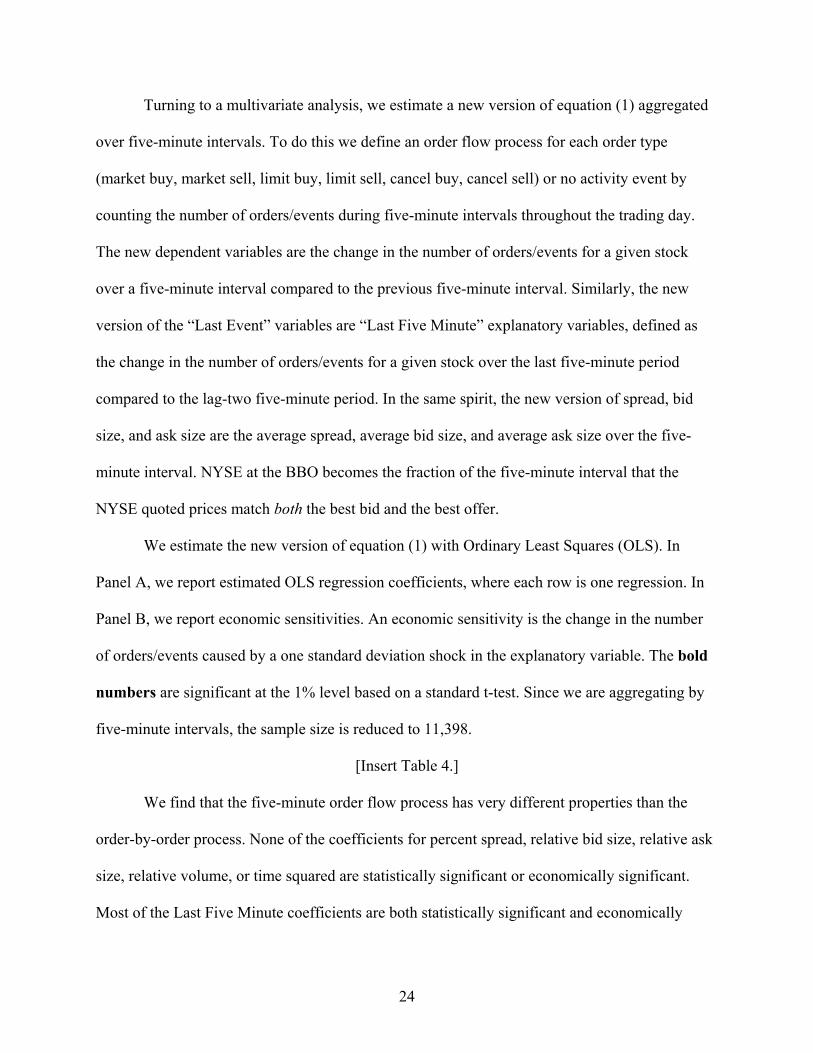
Turning to a multivariate analysis, we estimate a new version of equation (1) aggregated

over five-minute intervals. To do this we define an order flow process for each order type

(market buy, market sell, limit buy, limit sell, cancel buy, cancel sell) or no activity event by

counting the number of orders/events during five-minute intervals throughout the trading day.

The new dependent variables are the change in the number of orders/events for a given stock

over a five-minute interval compared to the previous five-minute interval. Similarly, the new

version of the “Last Event” variables are “Last Five Minute” explanatory variables, defined as

the change in the number of orders/events for a given stock over the last five-minute period

compared to the lag-two five-minute period. In the same spirit, the new version of spread, bid

size, and ask size are the average spread, average bid size, and average ask size over the five-

minute interval. NYSE at the BBO becomes the fraction of the five-minute interval that the

NYSE quoted prices match both the best bid and the best offer.

We estimate the new version of equation (1) with Ordinary Least Squares (OLS). In

Panel A, we report estimated OLS regression coefficients, where each row is one regression. In

Panel B, we report economic sensitivities. An economic sensitivity is the change in the number

of orders/events caused by a one standard deviation shock in the explanatory variable. The bold

numbers are significant at the 1% level based on a standard t-test. Since we are aggregating by

five-minute intervals, the sample size is reduced to 11,398.

[Insert Table 4.]

We find that the five-minute order flow process has very different properties than the

order-by-order process. None of the coefficients for percent spread, relative bid size, relative ask

size, relative volume, or time squared are statistically significant or economically significant.

Most of the Last Five Minute coefficients are both statistically significant and economically

25

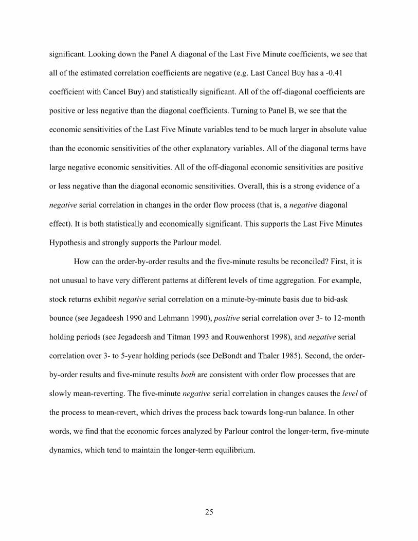
significant. Looking down the Panel A diagonal of the Last Five Minute coefficients, we see that

all of the estimated correlation coefficients are negative (e.g. Last Cancel Buy has a -0.41

coefficient with Cancel Buy) and statistically significant. All of the off-diagonal coefficients are

positive or less negative than the diagonal coefficients. Turning to Panel B, we see that the

economic sensitivities of the Last Five Minute variables tend to be much larger in absolute value

than the economic sensitivities of the other explanatory variables. All of the diagonal terms have

large negative economic sensitivities. All of the off-diagonal economic sensitivities are positive

or less negative than the diagonal economic sensitivities. Overall, this is a strong evidence of a

negative serial correlation in changes in the order flow process (that is, a negative diagonal

effect). It is both statistically and economically significant. This supports the Last Five Minutes

Hypothesis and strongly supports the Parlour model.

How can the order-by-order results and the five-minute results be reconciled? First, it is

not unusual to have very different patterns at different levels of time aggregation. For example,

stock returns exhibit negative serial correlation on a minute-by-minute basis due to bid-ask

bounce (see Jegadeesh 1990 and Lehmann 1990), positive serial correlation over 3- to 12-month

holding periods (see Jegadeesh and Titman 1993 and Rouwenhorst 1998), and negative serial

correlation over 3- to 5-year holding periods (see DeBondt and Thaler 1985). Second, the order-

by-order results and five-minute results both are consistent with order flow processes that are

slowly mean-reverting. The five-minute negative serial correlation in changes causes the level of

the process to mean-revert, which drives the process back towards long-run balance. In other

words, we find that the economic forces analyzed by Parlour control the longer-term, five-minute

dynamics, which tend to maintain the longer-term equilibrium.

26

4.3. Separating Auto-ex Orders from Floor Orders In Table 5, we separately consider orders routed to the automatic execution system

(Direct+) and orders routed to the floor. Specifically, the marketable order types are subdivided

into auto-ex or floor. Thus, we estimate a 9-way event model: (1) cancel buy; (2) cancel sell; (3)

limit buy order; (4) limit sell order; (5) floor marketable buy; (6) floor marketable sell; (7) auto-

ex marketable buy; (8) auto-ex marketable sell; and, (9) no activity. We pool data across stocks

for this regression. Due to the large number of observations with this approach, all of the

impulse sensitivities are statistically significant.

[Insert Table 5.]

Panel A shows the impulse sensitivities for the 9-way event model. The most striking

result is that the impulse sensitivities of the auto-ex orders are much smaller than those of the

floor orders. To see how much smaller they are, Panel B shows the value of the floor impulse

sensitivity relative to the auto-ex impulse sensitivity. The median ratio for marketable buys is 69

and the median ratio for marketable sells is 140. Auto-ex orders are very insensitive to market

conditions; whereas floor orders have economically meaningful regard for market conditions.

This supports the proposition that extremely impatient traders submit auto-ex orders, whereas

moderately impatient traders submit marketable floor orders.

4.4 Robustness

As one robustness check, we re-estimate the 7-way event structure and the 13-way event

structure using data from the first day of our sample (April 3) and again using the last day of our

sample (June 27). These results, which we do not report, are strongly similar to the results in

Tables 2 and 3.17 In all of the reported robustness checks below, we re-estimate equation (1)

17 We also perform a non-reported robustness check for potential endogeneity problems. It is possible that contemporaneous volume, quotes and volatility might be co-determined. To address this we use an instrument for

27

using pooled data. That is, we do not estimate equation (1) separately for each stock. Our

pooled regression has sufficient observations so that all regression coefficients and impulse

sensitivities are different from zero at traditional significance levels. Therefore, we do not report

significance levels. We only discuss when the conclusions differ from the results presented in the

previous section. In order to save space, we report only the impulse sensitivities.

4.4.1 Order Size

Table 6 provides the impulse sensitivities resulting from re-estimating equation (1)

conditional on the size of the order. We arbitrarily construct three order-size categories. Small

orders are defined as orders of fewer than 1,000 shares. Medium orders range between 1,000

and 9,999 shares. Large orders exceed 9,999 shares. We pool (across stocks) all orders in the

given size categories for each re-estimation.

[Insert Table 6.]

An interesting finding comes from testing the spread hypothesis by order size. We find

that a wide spread greatly increases (decreases) small limit (market) orders, moderately increases

(decrease) medium limit (market) orders, but has little effect on large limit (market) orders. This

is probably because a large order size dwarfs the quoted depth and so the quoted spread is a far

less relevant predictor of trading cost for these orders. In general, we note that most of the

impulse sensitivities are smaller for large orders. This is especially true for large limit orders.

4.4.2 Volume and Price Level

Recall that 100 of our sample securities are selected to provide cross-sectional dispersion

across trading volume and security price. As a robustness check, we re-estimate the logit model

conditioning on volume and price. Table 7 shows these results. Panel A pools the data from the

the volume in the previous five-minute interval. The instrument we use is the volume in the five-minute interval prior to the previous five-minute interval (i.e., t-2). This alternative specification does not alter our conclusions in any meaningful manner.

28

50 most active stocks. Panel B’s (C’s) impulse sensitivities result from examining the high-

volume:high-priced (:low-priced) stocks. Finally Panel D pools the low-volume stocks’ data.

Pooling all 50 low volume stocks is necessary to obtain convergence of the maximum likelihood

estimation of equation (1).

[Insert Table 7.]

Although the results generally are strongest for the higher volume subsets, most conclusions are

consistent across the various volume-price groups. A few exceptions are evident. For the low-

volume stocks, we find that the likelihood of marketable orders falls as the volume and volatility

in the prior five-minute interval increases. This might suggest that market orders in low-volume

stocks are subject to sloppy executions in difficult markets. The Volatility Hypothesis (of

Foucault, 1999) is supported for the low-volume stocks. In addition, the likelihood of limit buy

(sell) orders increases (decreases) as the market return from the previous five-minute interval

increases for the low price and lowest-volume stocks. For the lowest-volume stocks, there is

some evidence consistent with the claim that traders switch from limit to market orders as the

day passes. Finally, the largest impulse sensitivity with the Last Event Market Buy (Sell) is

associated with limit buy (sell) orders in all but the highest volume stocks, suggesting that as

liquidity is extinguished on one side of the book liquidity is added on the opposite side.

4.4.3 Order Splitting and End-of-Day Effects

We perform additional robustness checks on the 7-way event structure and report the

results in Table 8. We allow for the possibility that traders split orders in Panel A, and determine

if differences in order choice emerge toward the close of the trading day in Panel B.

[Insert Table 8.]

29

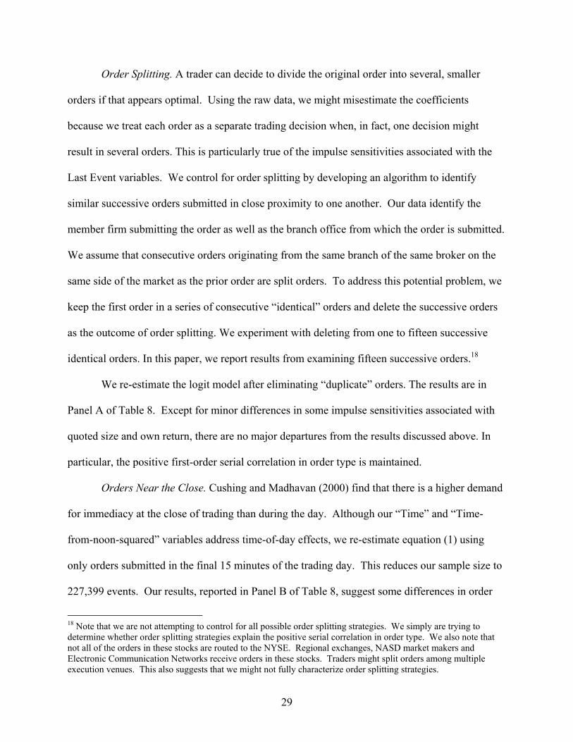
Order Splitting. A trader can decide to divide the original order into several, smaller

orders if that appears optimal. Using the raw data, we might misestimate the coefficients

because we treat each order as a separate trading decision when, in fact, one decision might

result in several orders. This is particularly true of the impulse sensitivities associated with the

Last Event variables. We control for order splitting by developing an algorithm to identify

similar successive orders submitted in close proximity to one another. Our data identify the

member firm submitting the order as well as the branch office from which the order is submitted.

We assume that consecutive orders originating from the same branch of the same broker on the

same side of the market as the prior order are split orders. To address this potential problem, we

keep the first order in a series of consecutive “identical” orders and delete the successive orders

as the outcome of order splitting. We experiment with deleting from one to fifteen successive

identical orders. In this paper, we report results from examining fifteen successive orders.18

We re-estimate the logit model after eliminating “duplicate” orders. The results are in

Panel A of Table 8. Except for minor differences in some impulse sensitivities associated with

quoted size and own return, there are no major departures from the results discussed above. In

particular, the positive first-order serial correlation in order type is maintained.

Orders Near the Close. Cushing and Madhavan (2000) find that there is a higher demand

for immediacy at the close of trading than during the day. Although our “Time” and “Time-

from-noon-squared” variables address time-of-day effects, we re-estimate equation (1) using

only orders submitted in the final 15 minutes of the trading day. This reduces our sample size to

227,399 events. Our results, reported in Panel B of Table 8, suggest some differences in order

18 Note that we are not attempting to control for all possible order splitting strategies. We simply are trying to determine whether order splitting strategies explain the positive serial correlation in order type. We also note that not all of the orders in these stocks are routed to the NYSE. Regional exchanges, NASD market makers and Electronic Communication Networks receive orders in these stocks. Traders might split orders among multiple execution venues. This also suggests that we might not fully characterize order splitting strategies.

30

choice. The impulse sensitivities associated with our quoted size variables indicate that traders

appear less willing to join a queue when the end of trading is near. When bid (ask) size is large,

traders are less likely to submit buy (sell) limit orders. There also is less evidence of momentum

trading in the last 15 minutes of trading. Finally, the time and time squared variables suggest

less trading at the end of our 15-minute interval than at the beginning.19

5. Conclusion

This paper analyzes the trader’s order choice decision across different securities and

under different market conditions for a sample of 148 stocks trading on the NYSE. We estimate

a multinomial logit model of order choice to perform a comprehensive test of order choice

theory. Our main results are: (1.) negative autocorrelations in changes in the order flow processes

over five minute intervals supporting dynamic limit order book theory, despite positive first-

order autocorrelation in order type; (2.) orders routed to an automatic execution system are much

less sensitive to market conditions than orders routed to the floor supporting an extreme

impatience theory of automatic execution customers; (3.) wider (narrower) spreads increase the

probability of small limit (marketable) orders, but have a negligible effect on large limit

(marketable) orders; (4.) large ask (bid) depth increases the probability of sells (buys) supporting

a short-term forecast hypothesis; (5.) large ask (bid) depth increases the probability of an inside-

the-quote limit sell (buy) and decreases the probability of an at-the-quote or behind-the-quote

limit sell (buy) supporting a “jump the queue” hypothesis; (6.) favorable (unfavorable) forecasts

of the rest-of-the-day stock return increase the likelihood of buy (sell) orders providing direct

evidence of effective private information trading; (7.) positive (negative) last-five-minute market

returns generate more buy (sell) orders indicating momentum-oriented technical trading; (8.)

order activity is clustered; (9.) doing nothing, defined as the passage of time without order 19 Eliminating time and time-from-noon-squared does not change our conclusions on the other variables.

31

activity, is clustered; and (10.) aggressively priced limit orders are more likely late in the trading

day providing evidence in support of prior experimental results.

As with all empirical studies, several caveats are in order. First, we note that our

empirical design captures individual orders, not complete order strategies. Although we adjust

for a simple form of order splitting, we cannot anticipate all possible strategies. We also note that

all strategies are not equally available to all traders. For example, the model might suggest that

an order be cancelled, but we cannot observe that outcome if an order has not been previously

placed. Third, we have only NYSE order data. Without data from all venues trading NYSE-listed

securities, we cannot fully characterize order choice. During our sample period 83% of the

sample stocks traders (86% of the volume) occurred on the NYSE. Finally, we focus exclusively

on electronically-submitted (system) orders. We do not have access to most orders originally

routed to a floor broker instead of the specialist.

Our results have implications for traders, trading venues, and regulators. Traders that

demand liquidity can adapt their order submissions to maximize the likelihood their orders will

fill at minimum cost. Liquidity suppliers can access the competition they are likely to face and

the profitability of their orders. Exchange and regulators can use these results when suggesting

alterations in trading mechanisms and rules.

32

Appendix: Testing The Statistical Significance of an Impulse sensitivity

Let π̂ be a vector of unrestricted reduced form parameter estimates and Ψ be the

covariance matrix of the parameter estimates π̂ . Let ( )h π be a r -dimensional set of r

restrictions, which are nonlinear in π , and ( ) /′= ∂ ∂H h π π . For a sample size T , the Wald test

statistic

( ) ( ) ( )1ˆ ˆq T −′ ′= h π H ΨH h π

is asymptotically 2( )rχ and is asymptotically equivalent to a likelihood ratio test (see Byron, 1974

and Judge et al, 1985, pgs 615-616).

We apply the Wald technique to calculate the statistical significance of an impulse

sensitivity, where the unrestricted reduced form parameter estimates arise from a multinomial

logit. An impulse sensitivity is the change in probability of a particular dependent variable

caused by a one standard deviation shock in an independent variable.

Let 1, 2, ,i I= K index the dependent variables, excluding the base case variable. Let

1, 2, ,j J= K index the independent variables, including the intercept. Stack the I x J reduced

form estimated coefficients into a (1x IJ ) vector c in ji order.20

Let ja and jb be the mean and standard deviation of the jth independent variable.21 Insert

these values into (1x IJ ) vectors to create I vectors im and IJ vectors jis as shown below. For

example, here are 1m , 2m , 11s , 21s , 12s , and 22s

20 The ji order matches the SAS ordering of outputs from a multinomial logit. 21 As one of the dependent variables, the intercept has a mean of 1 and a standard deviation of 0.

33

1 1 1 1

1

2 2 2 21 2 11 21

2

00 0 0

elements in 0 0 0 0

each partition0 0 0 0

0 0 0 partitions0 0 00 0 0

a a b aa

I

a a a ba J

+

+= = = =

m m s s

M M M

1 1 1

12 22

2 2 2

0 0

0 00 00 0 .

00 0 00 0 0

a b a

a a b

+ = =

+

s s

M M M

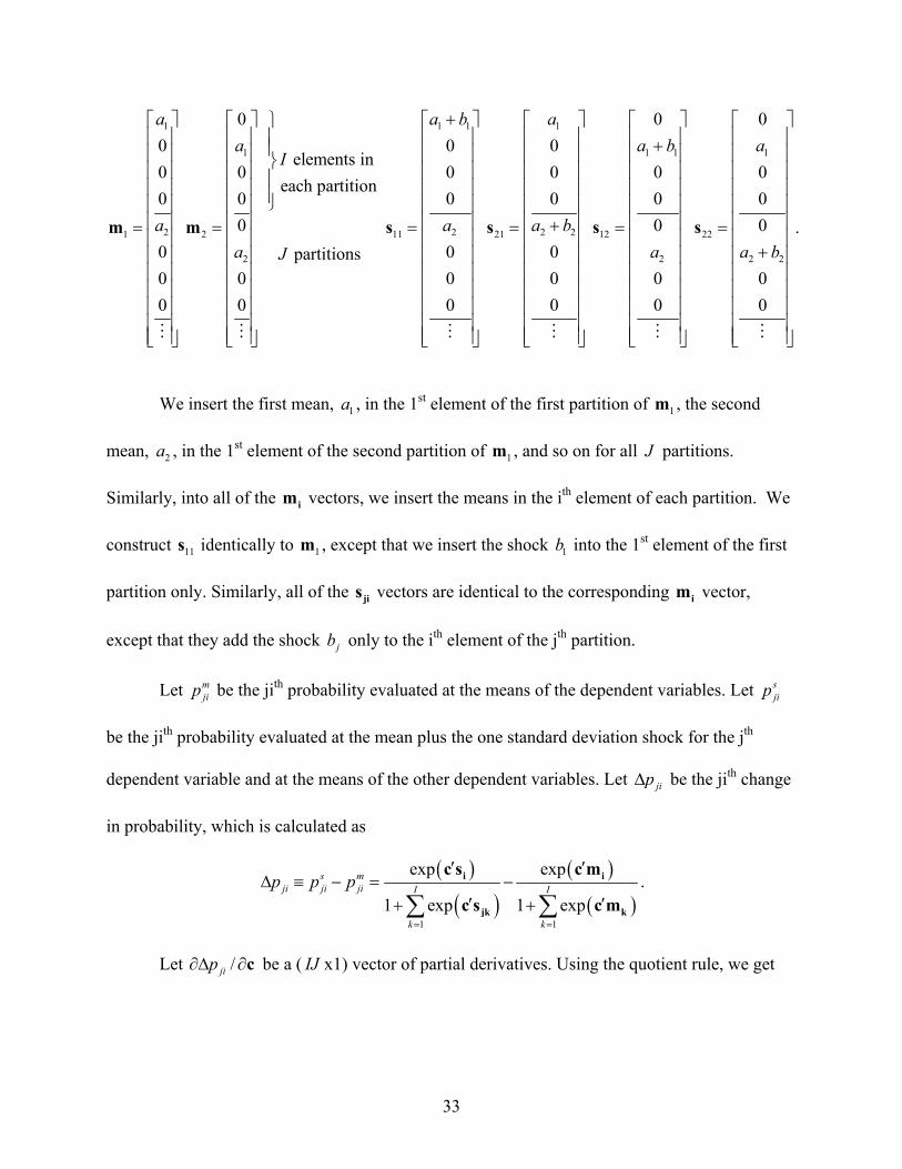
We insert the first mean, 1a , in the 1st element of the first partition of 1m , the second

mean, 2a , in the 1st element of the second partition of 1m , and so on for all J partitions.

Similarly, into all of the im vectors, we insert the means in the ith element of each partition. We

construct 11s identically to 1m , except that we insert the shock 1b into the 1st element of the first

partition only. Similarly, all of the jis vectors are identical to the corresponding im vector,

except that they add the shock jb only to the ith element of the jth partition.

Let mjip be the jith probability evaluated at the means of the dependent variables. Let s

jip

be the jith probability evaluated at the mean plus the one standard deviation shock for the jth

dependent variable and at the means of the other dependent variables. Let jip∆ be the jith change

in probability, which is calculated as

( )

( )( )

( )1 1

exp exp

1 exp 1 exp

s mji ji ji I I

k k

p p p

= =

′ ′∆ ≡ − = −

′ ′+ +∑ ∑i i

jk k

c s c m

c s c m.

Let /jip∂∆ ∂c be a ( IJ x1) vector of partial derivatives. Using the quotient rule, we get

34

( ) ( ) ( ) ( )

( )

( ) ( ) ( ) ( )

( )

1 12

1

1 12

1

exp 1 exp exp exp

1 exp

exp 1 exp exp exp .

1 exp

I I

ji k k

I

k

I I

k k

I

k

p = =

=

= =

=

′ ′ ′ ′⋅ + − ⋅ ∂∆ =∂ ′+

′′ ′ ′ ′⋅ + − −

′+

∑ ∑

∑

∑ ∑

∑

ji ji jk ji jk jk

jk

i i k i k k

k

s c s c s c s s c s

cc s

m c m c m c m m c m

c m

We test a single ( )1r = , cross-equation restriction 0jip∆ = . Using the covariance matrix

Ψ 22 of the reduced form parameter estimates c with a sample size of T , the Wald test statistic

( ) ( )1

ji jiji ji

p pq T p p

− ′∂∆ ∂∆ = ∆ ∆ ∂ ∂

Ψc c

is asymptotically distributed 2(1)χ .

For the base case dependent variable, the jth change in probability is

( ) ( )1 1

1 1

1 exp 1 exp

s mj j j I Ip p p

= =

∆ ≡ − = −′ ′+ +∑ ∑jl l

l l

c s c m.

For the base case dependent variable, the ( IJ x1) vector of partial derivatives /jp∂∆ ∂c is

( )

( )

( )

( )

1 12 2

1 1

exp exp .

1 exp 1 exp

I I

j k k

I I

k k

p= =

= =

′′ ′− ⋅∂∆= +

∂ ′ ′+ +

∑ ∑

∑ ∑

jk jk k k

jk k

s c s m c m

cc s c m

For the single restriction 0jp∆ = using the same covariance matrix Ψ , the Wald statistic

( ) ( )1

j jj j

p pq T p p

− ′∂∆ ∂∆ = ∆ ∆ ∂ ∂

Ψc c

is asymptotically distributed 2(1)χ .

22 See Maddala (1999), page 37 for details on how to calculate the covariance matrix Ψ in a multinomial logit.

35

References

Ahn, H., K. Bae, and K. Chan, 2001, “Limit Orders, Depth, and Volatility,” Journal of

Finance 56, 767-88.

Bae, K-H., H. Jang, and K. Park, 2002, “Traders’ Choice between Limit and Market Orders:

Evidence from NYSE Stocks,” Journal of Financial Markets, forthcoming.

J. Bacidore, R. Battalio, and R. Jennings, 2003, “Order Submission Strategies, Liquidity Supply,

and Trading in Pennies on the New York Stock Exchange,” Journal of Financial Markets

6, 337-362.

Belsley, D. A., E. Kuh, and R. E. Welsch, 1980, Regression Diagnostics, Wiley Publishing, New

York.

Beber, A., and C. Caglio, 2002, “Orders Submission Strategies and Information: Empirical

Evidence from the NYSE,” unpublished paper, University of Pennsylvania.

Biais, B., P. Hillion, and C. Spatt, 1995, “An Empirical Analysis of the Limit-order Book

and the Order Flow in the Paris Bourse,” Journal of Finance 50, 1655-89.

Bloomfield, R., M. O’Hara, and G. Saar, 2002, “The ‘Make or Take’ Decision in an

Electronic Market: Evidence on the Evolution of Liquidity,” Unpublished paper,

Cornell University.

Brown, D. and R. Jennings, 1990, “On Technical Analysis,” Review of Financial Studies 2, 527-

552.

Byron, R. P., 1974, “Testing Structural Specification Using the Unrestricted Reduced Form,”

Econometrica, 42, 869-84.

Chung, K., B. Van Ness, and R. Van Ness, 1999, “Limit Orders and the Bid-Ask Spread,”

Journal of Financial Economics 53, 255-87.

36

Cohen, K., S. Maier, R. Schwartz, and D. Witcomb, 1981, “Transactions Costs, Order

Placement Strategy, and Existence of the Bid-Ask Spread,” Journal of Political

Economy 89, 287-305.

Cushing, D., and A. Madhavan, 2000, “Stock Returns and Trading at the Close,” Journal of

Financial Markets 3, 45-62.

Danielsson, J., and R. Payne, 2002, “Measuring and Explaining Liquidity on an Electronic Limit

Order Book: Evidence from Reuters D2000-2,” unpublished paper, Financial Markets

Group, London School of Economics.

De Bondt, W. and R. Thaler, 1985, “Does the Stock Market Overreact?” Journal of Finance 40,

793–805.

Easley, D., N. Kiefer, and M. O’Hara, 1997, “One Day in the Life of a Very Common

Stock,” Review of Financial Studies, 10, 805-35.

Ellul, A., C. Holden, P. Jain, and R. Jennings, 2003, “Optimal Intertemporal Order Strategy,”

Indiana University working paper.

Foucault, T., 1999, “Order Flow Composition and Trading Costs in a Dynamic Limit Order

Market,” Journal of Financial Markets 2, 99-134.

Gencay, R., 1998, “The Predictability of Security Returns With Simple Technical Trading

Rules,” Journal of Empirical Finance 5, 347-359.

Handa, P., and R. Schwartz, 1996, Limit Order Trading, Journal of Finance 51, 1835-61.

Harris, L., 1998, “Optimal Dynamic Order Submission Strategies in Some Stylized

Trading Problems,” Financial Markets, Institutions, and Instruments 7, 1-75.

Harris, L., and J. Hasbrouck, 1996, “Market versus Limit Orders: the SuperDOT Evidence on

Order Submission Strategy,” Journal of Financial and Quantitative Analysis 31, 212-31.

37

Hasbrouck, J., and G. Saar, 2002, “Limit Orders and Volatility in a Hybrid market: The Island

ECN,” unpublished paper, New York University.

Hollifield, B., R. Miller, and P. Sandås, 1999, “An Empirical Analysis of Limit Order

Markets,” Unpublished paper, Rodney White Center for Financial Research

Working Paper 029-99, University of Pennsylvania.

Hollifield, B., R. Miller, P. Sandås, and J. Slive, 2002, “Liquidity Supply and Demand in Limit

Order Markets,” Unpublished paper, Rodney White Center for Financial Research

Working Paper, University of Pennsylvania.

Jegadeesh, N., 1990, “Evidence of Predictable Behavior of Security Returns,” Journal of

Finance 45, 881–98.

Jegadeesh, N. and S. Titman, 1993, “Returns to Buying Winners and Selling Losers:

Implications for Market Efficiency,” Journal of Finance 48, 65–92.

Judge, G.G., W.E. Griffiths, R.C. Hill, H. Lutkepohl, and T.C. Lee, 1985, The Theory and

Practice of Econometrics, John Wiley and Sons, New York.

Kavajecz, K., 1999, “A Specialist’s Quoted Depth and the Limit Order Book,” Journal of

Finance 54, 747-72.

Lehmann, B., 1990, “Fads, Martingales, and Market Efficiency,” Quarterly Journal of

Economics 105, 1–28.

Lo, A., H. Mamaysky, and J. Wang, 2000, “Foundations of Technical Analysis: Computational

Algorithms,” Journal of Finance 55, 1705-1765.

Maddala, G.S., 1999, Limited-Dependent and Qualitative Variables in Econometrics,

Cambridge University Press, Cambridge.

38

Parlour, C., 1998, “Price Dynamics in Limit Order Markets,” Review of Financial Studies

11, 789-816.

Peterson, M., and E. Sirri, 2000, “Order Submission Strategy and the Curious Case of

Marketable Limit Orders,” Journal of Financial and Quantitative Analysis 37, 221-41.

Ranaldo, A., 2002, “Order Aggressiveness in Limit Order Book Markets,” Journal of

Financial Markets, forthcoming.

Ready, M., 2002, “Profits from Technical Trading Rules,” Financial Management 31, 43-61.

Roth, A., K. Murnigham, and F. Schoumaker, 1988, “The Deadline Effect in Bargaining: Some

Experimental Evidence,” American Economic Review 78, 806-23.

Rouwenhorst, G., 1998, “International Momentum Strategies,” Journal of Finance 53, 267–84.

Sandås, P., 2001, “Adverse Selection and Competitive Market Making: Empirical Evidence from

a Pure Limit Order Market,” Review of Financial Studies 14, 705-34.

Seppi, D., 1997, “Liquidity Provision with Limit Orders and a Strategic Specialist,” Review of

Financial Studies 10, 103-50.

Smith, J., 2000, “Market versus Limit Order Submission Behavior at a Nasdaq Market

Maker,” Unpublished paper, Nasdaq Economic Research.

Sullivan, R., A. Timmerman, and H. White, 1999, “Data-Snooping, Technical Trading Rule

Performance, and the Bootstrap,” Journal of Finance 54, 1647-1691.

Swinscow, T., 1997, Statistics at Square One, 9th edition, London, BMJ Publishing.

United States Securities and Exchange Commission, 2001, Report on Comparison of Order

Executions Across Equity Market Structures, Office of Economic Analysis.

United States Securities and Exchange Commission, 2001, “Disclosure of Order Execution and

Routing Practices.”

39

Yeo, W., 2002, “Persistent Pattern in Limit Order Submission,” unpublished paper, Indiana

University.

40

Table 1. Descriptive Statistics

The Table reports descriptive statistics for the sample of 148 stocks trading on the New York Stock Exchange during the week of April 30 – May 4, 2001. Order size is the pooled time series cross-sectional average of the number of shares submitted in orders. Daily share volume is the pooled time series cross-sectional average of the volume in shares transacted. The shares outstanding variable is the volume weighted average of the shares outstanding for the firms in the sample. The National Best Bid Size is the size associated with the lowest bid price across all markets quoting the stock. The National Best Offer Size is the size associated with the highest ask price across all markets quoting the stock. Percent spread is the national best bid-ask spread divided by the average of the national best bid price and the national best ask price. Time is the number of five-minute intervals since midnight. Own return is the change in the midpoint of the security’s bid-ask spread over the five minutes prior to the order arrival or cancellation. Market return is the change in the midpoint of the midpoint of the bid-ask spread of the exchange traded fund representing the Exchange Traded Fund tracking the S&P500 Index. Private information variable is measured as [(closing quote midpoint) - (order-time quote midpoint)/(order-time quote midpoint)]. Variable Mean Std.

Deviation Minimum Maximum

Order size 1,231.88 5,501.62 100 900,000 Daily share volume 2,242,779 1,555,359 555 6,454,023 Shares outstanding (in 000) 2,118,639 1,942,579 61 9,932,929 National Best Bid Size (’00) 27.60 68.57 1 5,880 National Best Offer Size (’00) 37.01 103.59 1 8,376 Spread midpoint ($) 43.80 23.04 0.525 118.9 Spread ($) 0.0523 0.0492 0.00 6.14 Percent spread 0.15 0.20 0.00 26.15 Last Event Market Buy 0.1250 0.3306 0 1 Last Event Market Sell 0.1266 0.3320 0 1 Last Event Limit Buy 0.1641 0.3702 0 1 Last Event Limit Sell 0.1546 0.3615 0 1 Time 153.76 24.52 114 192 Own Return 0.000141 0.009252 -0.086896 0.106667 Market Return 0.000058 0.001043 -0.002974 0.004434 Private information 0.002676 0.015272 -0.121806 0.249431

41

Table 2. Estimation of the 7-Way Event Structure on a Stock-By-Stock Basis

The table reports the results from estimating equation (1). In Panel A, we report the estimated regression coefficients. In Panel B, we report the impulse sensitivities (change in the probability of an event caused by a one standard deviation shock in the explanatory variable). In each panel we report the mean from 86 regressions. For 85 of our sample stocks, the maximum likelihood estimation of equation (1) converges. For the other sample stocks, we pool data into an eighty-sixth regression. Event

Last Can. Buy

Last Can. Sell

Last Limit Buy

Last Limit Sell

Last Mkt. Buy

Last Mkt. Sell

Percent Spread

Rel. Bid Size

Rel. Ask Size

Rel. Vol.

Own Ret.

Own Ret. Sqr.

Mkt. Ret.

Time

Time Sqr.

Private Infor-mation

NYSE Not At NBBO

Panel A: Mean Estimated Regression Coefficients Cancel Buy 1.773 1.045 1.560 1.016 1.005 0.876 39.28 -1.041 -0.200 0.99 45.308 1.36 82.925 0.068 .380 2.085 0.288 Cancel Sell 0.888 1.712 1.002 1.512 0.735 1.095 36.70 -0.108 -0.558 1.15 -25.53 1.54 -70.07 -2.006 .419 0.406 0.352 Limit Buy 1.506 1.101 1.354 0.924 0.951 0.865 136.46 0.574 -0.318 1.32 2.442 1.47 81.602 1.905 .404 7.154 0.346 Limit Sell 1.114 1.520 0.960 1.317 0.842 .0997 154.9 -0.362 0.399 1.41 18.010 1.49 -84.91 0.837 .443 -10.53 0.387 Market Buy 0.757 0.570 0.674 0.575 1.089 0.469 -132.8 0.835 -0.018 1.17 90.639 1.67 121.96 1.074 .768 9.068 0.286 Market Sell 0.504 0.855 0.612 0.732 0.647 1.074 -114.0 0.207 0.611 0.77 -104.8 1.14 -105.4 -0.043 .719 -12.90 0.170 Panel B: Mean Impulse Sensitivities (%) Cancel Buy 2.41 0.812 2.21 0.83 0.80 0.45 0.04 -0.32 -0.16 0.14 0.57 0.51 0.47 -0.07 0.20 0.01 0.26 Cancel Sell 0.83 2.171 0.71 2.08 0.32 0.83 0.06 -0.14 -0.39 0.14 -0.57 0.52 -0.34 -0.16 0.42 -0.12 0.28 Limit Buy 2.72 1.023 3.93 1.18 1.31 0.80 3.17 0.69 -0.41 0.38 1.08 0.64 0.28 0.48 0.63 0.71 0.49 Limit Sell 0.99 2.559 1.02 3.40 0.73 1.18 3.50 -0.39 0.55 0.48 -1.13 1.04 -0.38 0.38 0.79 -0.75 0.66 Market Buy 0.01 -0.263 0.15 -0.12 1.58 0.12 -2.13 0.48 0.01 0.31 1.57 0.40 0.64 0.068 1.64 0.40 0.02 Market Sell -0.23 0.166 -0.09 0.26 0.21 1.87 -1.98 0.04 0.34 0.21 -1.34 0.45 -0.35 -0.23 1.53 -0.60 0.13 No Activity -6.74 -6.468 -7.95 -7.64 -4.98 -5.27 -2.67 -0.36 0.06 -1.70 -0.59 -3.60 -0.10 -0.45 -5.20 0.36 -1.86 Panel C: Hypothesis Predicted Signs of the Impulse Sensitivities Cancel Buy + + Cancel Sell + + Limit Buy + - + + + - + + ≠0 + + + Limit Sell + - + + + + + - ≠0 + - + Market Buy - - + + - - + ≠0 + + Market Sell - - + + + - - ≠0 + - No Activity - - Coefficients for bid size, ask size, time, and time squared are multiplied by 1,000. Coefficients for relative volume (own return squared) are multiplied by 1,000,000 (10,000). Bold numbers are significant at the .01 level with both a standard cross-sectional t-test and a Chi-square test of proportions using the 86 regressions on the regression coefficient estimates in Panel A and the impulse sensitivities in Panel B. The test of proportions tests the null hypothesis that significantly more than one-half of the individual coefficient estimates (in Panel A) or impulse sensitivities (in Panel B) have the same sign as the mean.

42

Table 3. Estimation of the 13-Way Event Structure on a Stock-By-Stock Basis

The table reports the results from estimating equation (1). In Panel A, we report the estimated regression coefficients. In Panel B, we report the impulse sensitivities (change in the probability of an event caused by a one standard deviation shock in the explanatory variable). In each panel we report the mean from 86 regressions. For 85 of our sample stocks, the maximum likelihood estimation of equation (1) converges. For the other sample stocks, we pool data into an eighty-sixth regression.

Event

Last Can. Buy

Last Can. Sell

Last Limit Buy

Last Limit Sell

Last Mkt. Buy

Last Mkt. Sell

Percent Spread

Rel. Bid Size

Rel. Ask Size

Rel. Vol.

Own Ret.

Own Ret. Sqr.

Mkt. Ret.

Time

Time Sqr.

Private Infor-mation

NYSE Not At NBBO

Panel A. Regression Coefficient Estimates Cancel Buy 0.46 -4.69 2.44 -2.84 2.03 -4.06 48.51 -0.43 -0.43 0.96 12.13 1.40 36.44 -0.19 0.40 -1.77 0.22 Cancel Sell -4.61 0.33 -2.98 2.46 -4.3 2.15 56.49 -0.48 -0.26 1.08 5.23 1.44 -35.66 -0.54 0.42 -3.16 0.28 BTQ Limit Buy 1.26 1.15 1.51 1.20 0.82 0.84 7.21 -1.55 0.60 0.86 -3.68 0.93 1.15 0.08 0.74 8.12 0.08 ATQ Limit Buy 1.16 1.07 1.23 0.91 0.80 0.73 159.0 -0.87 -0.09 1.31 54.84 -1.81 104.9 3.65 0.27 4.66 0.20 ITQ Limit Buy 1.28 0.87 1.35 0.92 0.79 0.87 237.2 2.37 -2.05 1.28 6.21 0.90 115.8 2.67 0.30 9.34 0.24 ITQ Limit Sell 1.03 1.08 0.93 1.33 0.83 1.04 275.8 -1.85 1.64 0.98 16.65 0.90 -126.8 0.48 0.28 -11.16 0.31 ATQ Limit Sell 0.71 1.32 0.74 1.40 0.71 1.06 179.7 0.17 -0.37 1.19 38.43 1.30 -93.21 1.18 0.32 -14.01 0.27 BTQ Limit Sell 1.30 1.04 0.93 1.36 0.67 0.98 14.70 0.17 -1.02 0.96 -6.38 1.44 -4.20 4.04 0.84 -7.69 0.29 Mkt. Limit Buy 1.03 0.77 0.94 0.80 0.94 0.44 -468.3 1.89 -1.00 1.34 34.03 1.84 174.7 -0.09 0.69 9.28 0.20 Mkt. Limit Sell 0.51 1.06 0.44 0.78 0.84 1.38 -379.5 -0.74 1.27 1.20 -15.45 1.66 -131.1 -3.00 0.68 -16.58 -0.41 Market Buy 0.78 0.57 0.92 0.81 1.36 0.64 2.69 -0.35 0.29 1.01 65.28 1.16 123.8 2.78 0.79 5.10 -0.15 Market Sell 0.59 0.81 0.81 .093 0.61 1.40 -9.69 -0.46 0.32 -.49 -76.94 0.67 -146.3 1.47 0.72 -4.57 0.07 Panel B. Mean Impulse Sensitivities (%) Cancel Buy 0.04 -1.05 1.74 -1.15 1.06 -1.10 0.08 -0.04 -0.07 0.03 0.01 0.14 0.06 -0.04 0.08 0.01 0.08 Cancel Sell -0.93 0.05 -1.09 1.61 -1.02 1.05 0.02 -0.04 -0.05 0.04 0.01 0.14 -0.06 -0.04 0.10 -0.04 0.93 BTQ Limit Buy 1.17 1.07 1.45 0.92 0.51 0.50 -0.36 -0.37 0.29 0.12 -0.15 0.34 -0.00 -0.14 0.85 0.06 0.18 ATQ Limit Buy 1.09 0.02 1.80 0.44 0.65 0.41 1.07 -0.34 -0.14 0.10 -0.12 0.23 0.54 0.42 -0.06 0.27 0.14 ITQ Limit Buy 1.21 0.78 1.74 0.62 0.73 0.50 2.26 1.04 -1.07 0.22 0.10 0.17 0.80 0.32 0.37 0.57 0.29 ITQ Limit Sell 0.70 1.15 0.54 1.56 0.44 0.74 2.55 -0.78 0.96 0.20 0.14 0.12 -0.80 0.19 -0.08 -0.37 0.43 ATQ Limit Sell 0.55 0.98 0.40 1.53 0.44 0.55 1.17 -0.07 -0.23 0.16 0.28 0.31 -0.45 0.25 0.01 -0.43 0.22 BTQ Limit Sell 1.00 1.03 0.86 1.20 0.86 0.45 -0.10 0.14 -0.37 0.25 0.07 035 0.00 -0.02 1.01 -0.12 0.08 Mkt. Limit Buy 0.32 0.12 0.28 1.69 0.69 0.18 -1.64 0.27 -0.12 0.16 0.16 0.36 0.60 -0.11 0.57 0.24 0.05 Mkt. Limit Sell 0.22 0.39 0.19 0.34 0.23 0.78 -1.50 -0.02 0.23 0.19 0.01 0.39 -0.42 -0.28 0.56 -0.31 -0.10 Market Buy 0.59 0.23 0.60 0.39 1.60 0.46 -0.54 0.20 0.11 0.19 0.57 0.25 0.90 0.18 1.26 0.17 -0.02 Market Sell 0.25 0.67 0.42 0.69 0.50 1.90 -0.65 0.09 0.19 0.07 -0.37 0.35 -0.99 0.03 1.12 -0.29 0.14 No Activity -6.24 -6.08 -8.97 -8.97 -6.20 -6.47 -2.36 -0.06 0.28 -1.70 -0.72 -3.20 -0.17 0.74 -5.48 0.22 -1.60 BTQ = Behind-The-Quote; ATQ = At-The-Quote; ITQ = Inside-The-Quote. Coefficients for bid size, ask size, time, & time squared are multiplied by 1,000. Coefficients for relative volume & own return squared are multiplied by 1,000,000 & 10,000 respectively. Bold numbers are significant at the .01 level using a both a standard cross-sectional t-test and a Chi-square test of proportions using the 86 regressions on the regression coefficient estimates in Panel A and the impulse sensitivities in Panel B. The test of proportions tests the null hypothesis that significantly more than one-half of the individual coefficient estimates (in Panel A) or impulse sensitivities (in Panel B) are in the same direction as the mean.

43

Table 4. OLS Regressions of Orders / No Activity Events Aggregated Over Five Minute Intervals

The table reports the results from estimating equation (1) aggregated over five minute intervals. In Panel A, we report the estimated OLS regression coefficients, where each row is one OLS regression. In each row, the dependent variable is the change in number of orders or no activity events for a given stock over a five minute interval compared to the previous five minute interval. In Panel B, we report the economic sensitivities (change in the number of orders or no activity events caused by a one standard deviation shock in the explanatory variable).

OLS

Dependent Variable

Last 5 Min Can. Buy

Last 5 Min Can. Sell

Last 5 Min Limit Buy

Last 5 Min Limit Sell

Last 5 Min Mkt. Buy

Last 5 Min Mkt. Sell

Percent Spread

Rel. Bid Size

Rel. Ask Size

Rel. Vol.

Own Ret.

Own Ret. Sqr.

Mkt. Ret.

Time

Time Sqr.

Private Infor-mation

NYSE Not At NBBO

Panel A: Estimated OLS Regression Coefficients Cancel Buy -0.41 0.23 0.06 -0.10 0.11 -0.03 7.37 0.001 -0.006 -0.07 72 -147 1170 -60 0.37 88.97 -1.41 Cancel Sell 0.19 -0.37 -0.05 0.01 0.03 0.04 2.28 0.001 -0.008 -0.05 -227 61 -1986 -52 0.63 29.38 -0.62 Limit Buy 0.16 0.41 -0.43 -0.17 0.14 0.04 -0.38 0.003 -0.021 -0.18 -613 748 1292 -72 0.09 147.67 -0.44 Limit Sell 0.29 0.25 -0.01 -0.53 0.09 0.05 0.70 0.003 -0.025 -0.12 137 -324 -841 -55 0.10 43.60 2.54 Market Buy 0.05 0.45 0.02 -0.15 -0.30 0.06 -17.50 0.003 -0.019 -0.19 -722 755 2975 -41 0.06 199.90 -3.46 Market Sell 0.37 0.13 -0.13 -0.01 0.06 -0.39 -19.56 0.004 -0.036 -0.19 -245 107 -1658 -49 0.82 31.22 -2.58 No Activity 0.62 0.67 -0.21 -0.34 -0.11 0.04 -24.16 0.005 -0.040 -0.13 -133 111 -3214 -297 -1.69 186.78 -5.56 Panel B: Economic Sensitivities (Change in the Number of Orders or No Activity Events Caused By One Std Dev Shock in the Explanatory Variable) Cancel Buy -20.03 11.00 5.10 -8.34 8.88 -1.92 0.09 0.13 -0.10 -0.04 0.18 -0.23 0.57 -1.37 0.17 0.58 -0.25 Cancel Sell 9.21 -17.60 -4.11 0.78 2.27 2.76 0.03 0.15 -0.15 -0.03 -0.57 0.10 -0.98 -1.18 0.29 0.19 -0.11 Limit Buy 7.81 19.19 -37.19 -13.76 10.71 3.24 0.00 0.42 -0.38 -0.10 -1.53 1.19 0.63 -1.64 0.04 0.96 -0.08 Limit Sell 14.28 11.67 -0.53 -44.08 6.77 4.21 0.01 0.45 -0.46 -0.06 0.34 -0.51 -0.41 -1.24 0.04 0.28 0.45 Market Buy 2.31 21.01 1.56 -12.20 -23.92 4.44 -0.22 0.42 -0.34 -0.11 -1.80 1.20 1.46 -0.94 0.03 1.29 -0.61 Market Sell 18.35 6.20 -11.01 -1.07 4.75 -30.05 -0.25 0.63 -0.66 -0.10 -0.61 0.17 -0.81 -1.11 0.38 0.20 -0.46 No Activity 30.16 31.55 -17.86 -28.20 -8.59 3.11 -0.31 0.77 -0.73 -0.07 -0.33 0.18 -1.58 -6.72 -0.77 1.21 -0.98 Coefficients for bid size, ask size, time, and time squared are multiplied by 1,000. Coefficients for relative volume (own return squared) are multiplied by 1,000,000 (10,000).

Bold numbers are significant at the .01 level based on a standard t-test. The sample size is 11,398.

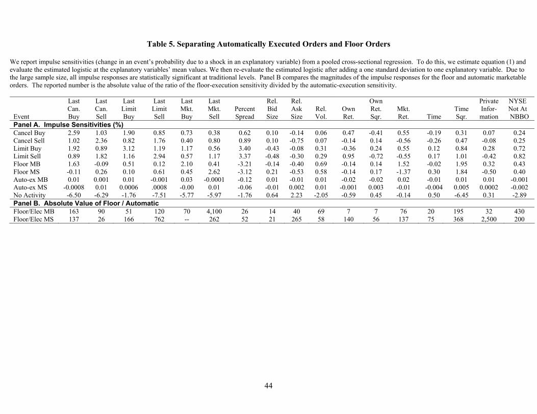
44

Table 5. Separating Automatically Executed Orders and Floor Orders

We report impulse sensitivities (change in an event’s probability due to a shock in an explanatory variable) from a pooled cross-sectional regression. To do this, we estimate equation (1) and evaluate the estimated logistic at the explanatory variables’ mean values. We then re-evaluate the estimated logistic after adding a one standard deviation to one explanatory variable. Due to the large sample size, all impulse responses are statistically significant at traditional levels. Panel B compares the magnitudes of the impulse responses for the floor and automatic marketable orders. The reported number is the absolute value of the ratio of the floor-execution sensitivity divided by the automatic-execution sensitivity.

Event

Last Can. Buy

Last Can. Sell

Last Limit Buy

Last Limit Sell

Last Mkt. Buy

Last Mkt. Sell

Percent Spread

Rel. Bid Size

Rel. Ask Size

Rel. Vol.

Own Ret.

Own Ret. Sqr.

Mkt. Ret.

Time

Time Sqr.

Private Infor-mation

NYSE Not At NBBO

Panel A. Impulse Sensitivities (%) Cancel Buy 2.59 1.03 1.90 0.85 0.73 0.38 0.62 0.10 -0.14 0.06 0.47 -0.41 0.55 -0.19 0.31 0.07 0.24 Cancel Sell 1.02 2.36 0.82 1.76 0.40 0.80 0.89 0.10 -0.75 0.07 -0.14 0.14 -0.56 -0.26 0.47 -0.08 0.25 Limit Buy 1.92 0.89 3.12 1.19 1.17 0.56 3.40 -0.43 -0.08 0.31 -0.36 0.24 0.55 0.12 0.84 0.28 0.72 Limit Sell 0.89 1.82 1.16 2.94 0.57 1.17 3.37 -0.48 -0.30 0.29 0.95 -0.72 -0.55 0.17 1.01 -0.42 0.82 Floor MB 1.63 -0.09 0.51 0.12 2.10 0.41 -3.21 -0.14 -0.40 0.69 -0.14 0.14 1.52 -0.02 1.95 0.32 0.43 Floor MS -0.11 0.26 0.10 0.61 0.45 2.62 -3.12 0.21 -0.53 0.58 -0.14 0.17 -1.37 0.30 1.84 -0.50 0.40 Auto-ex MB 0.01 0.001 0.01 -0.001 0.03 -0.0001 -0.12 0.01 -0.01 0.01 -0.02 -0.02 0.02 -0.01 0.01 0.01 -0.001 Auto-ex MS -0.0008 0.01 0.0006 .0008 -0.00 0.01 -0.06 -0.01 0.002 0.01 -0.001 0.003 -0.01 -0.004 0.005 0.0002 -0.002 No Activity -6.50 -6.29 -1.76 -7.51 -5.77 -5.97 -1.76 0.64 2.23 -2.05 -0.59 0.45 -0.14 0.50 -6.45 0.31 -2.89 Panel B. Absolute Value of Floor / Automatic Floor/Elec MB 163 90 51 120 70 4,100 26 14 40 69 7 7 76 20 195 32 430 Floor/Elec MS 137 26 166 762 -- 262 52 21 265 58 140 56 137 75 368 2,500 200

45

Table 6. Impulse Sensitivities (%) of the 7-Way Event Structure By Order Size

The table reports the impulse sensitivities (change in the probability of an event caused by a one standard deviation shock in the explanatory variable). To do this, we first estimate equation (1) and evaluate the estimated logistic equation at the mean value of all explanatory variables. We then re-evaluate the estimated logistic after adding a one standard deviation to one explanatory variable and report the change in the probability.

Event

Last Can. Buy

Last Can. Sell

Last Limit Buy

Last Limit Sell

Last Mkt. Buy

Last Mkt. Sell

Percent Spread

Rel. Bid Size

Rel. Ask Size

Rel. Vol.

Own Ret.

Own Ret. Sqr.

Mkt. Ret.

Time

Time Sqr.

Private Infor-mation

NYSE Not At NBBO

Panel A: Large Orders ( > 9,999 shares) Cancel Buy 0.04 0.02 0.04 0.03 0.02 0.02 0.01 0.002 -0.002 0.0009 0.03 -0.02 0.004 -0.003 0.06 -0.003 0.01 Cancel Sell 0.03 0.04 0.03 0.04 0.02 0.03 0.01 -0.09 0.002 0.007 -0.002 0.003 -0.01 -0.003 0.08 -0.004 0.01 Limit Buy 0.08 0.06 0.15 0.11 0.08 0.08 0.05 -0.07 0.004 0.02 -0.006 0.004 0.01 0.004 0.21 -0.008 0.04 Limit Sell 0.07 0.09 0.12 0.18 0.10 0.12 0.06 -0.36 -0.0001 0.03 -0.009 0.01 -0.01 0.02 0.28 -0.02 0.07 Market Buy 0.05 0.05 0.11 0.11 0.15 0.11 0.01 -0.11 0.003 0.02 0.21 -0.13 0.02 -0.02 0.24 0.02 0.02 Market Sell 0.04 0.05 0.08 0.09 0.09 0.14 0.03 -0.24 -0.02 0.03 -0.01 0.01 -0.04 -0.01 0.23 -0.03 0.02 No Activity -0.33 -0.35 -0.55 -0.57 -0.49 -0.52 -0.18 0.89 0.02 -0.10 -0.21 0.13 0.02 0.01 -1.13 0.05 -0.18 Panel B: Medium Orders (999 < shares < 10,000) Cancel Buy 1.10 0.57 0.94 0.55 0.48 0.36 0.75 -0.21 -0.27 0.23 0.13 -0.14 0.07 -0.10 0.57 0.03 0.22 Cancel Sell 0.64 1.17 0.62 1.02 0.41 0.58 0.82 -2.39 -0.04 0.22 -0.04 0.05 0.16 -0.08 0.67 -0.02 0.21 Limit Buy 1.30 0.85 1.88 1.19 0.98 0.82 0.18 -1.45 -0.79 0.61 -0.13 0.07 -0.19 0.13 1.54 0.06 0.73 Limit Sell 0.89 1.41 1.28 2.08 0.86 1.14 0.19 -1.19 -0.78 0.67 0.71 -0.54 0.09 0.18 1.62 -0.19 0.77 Mkt. Buy 0.52 0.35 0.80 0.57 1.61 0.62 -1.33 -0.93 -0.51 0.57 -0.03 0.04 -0.10 -0.19 1.61 0.15 0.44 Mkt. Sell 0.37 0.56 0.59 0.83 0.64 1.69 -1.31 -3.91 -0.23 0.55 0.05 0.07 0.81 -0.26 1.64 -0.28 0.44 No Activity -4.85 -4.94 -6.14 -6.26 -5.00 -5.23 -2.65 10.11 2.59 -2.87 -0.57 0.42 -0.65 0.32 -7.67 0.24 -2.84 Panel C: Small Orders ( < 1,000 shares) Cancel Buy 2.53 1.10 1.97 1.01 0.81 0.50 0.02 0.15 -0.13 0.05 0.54 -0.45 0.51 -0.17 0.37 0.04 0.31 Cancel Sell 1.03 2.18 0.91 1.72 0.46 0.82 0.37 0.53 -1.44 0.09 -0.13 0.11 -0.48 -0.25 0.46 -0.08 0.30 Limit Buy 1.96 1.08 3.16 1.37 1.29 0.70 2.01 -1.31 0.47 1.84 -0.29 0.20 0.60 -0.03 0.71 0.26 0.64 Limit Sell 1.06 1.74 1.27 2.77 0.64 1.17 1.91 -1.87 -0.06 0.004 0.89 -0.70 -0.60 -0.02 0.76 -0.36 0.70 Mkt. Buy 0.35 0.11 0.65 0.30 2.22 0.51 -2.62 -0.48 -0.48 0.49 -0.16 0.14 1.23 0.07 1.80 0.25 0.38 Mkt. Sell 0.07 0.42 0.27 0.74 0.52 2.40 -2.34 0.47 0.63 0.40 -0.11 0.13 -1.15 -0.17 1.63 -0.39 0.32 No Activity -7.03 -6.65 -8.26 -7.93 -5.95 -6.12 6.47 2.50 2.72 -1.24 -0.73 0.56 -0.11 0.56 -5.58 0.29 -2.68 .

46

Table 7. Impulse Sensitivities (%) of the 7-Way Event Structure By Volume and Price Category

The table reports the impulse sensitivities (change in the probability of an event caused by a one standard deviation shock in the explanatory variable) derived from equation (1) estimates.

Event

Last Can. Buy

Last Can. Sell

Last Limit Buy

Last Limit Sell

Last Mkt. Buy

Last Mkt. Sell

Percent Spread

Rel. Bid Size

Rel. Ask Size

Rel. Vol.

Own Ret.

Own Ret. Sqr.

Mkt. Ret.

Time

Time Sqr.

Private Infor-mation

NYSE Not At NBBO

Panel A: Highest Volume Stocks Cancel Buy 2.45 0.95 1.76 0.81 0.69 0.37 0.16 -0.28 -0.08 0.16 0.45 0.27 0.24 -0.19 0.27 0.10 0.26 Cancel Sell 0.94 2.25 0.79 1.62 0.39 0.75 0.26 -0.17 -0.24 0.13 -0.49 0.37 -0.18 -0.16 0.38 -0.12 0.26 Limit Buy 1.74 0.73 2.66 0.92 0.93 0.42 3.53 0.28 -0.15 0.41 0.83 0.29 -0.62 0.22 0.66 0.51 0.48 Limit Sell 0.68 1.56 0.85 2.40 0.42 0.93 3.61 -0.23 0.21 0.46 -0.74 0.42 0.72 0.39 0.62 -0.58 0.44 Mkt. Buy 0.07 -0.17 0.37 0.006 2.10 0.12 -2.24 0.47 - 0.41 1.82 0.55 0.06 -0.02 1.91 0.36 0.02 Mkt. Sell -0.20 0.15 -0.006 0.45 0.17 2.45 -2.17 0.03 0.44 0.27 -1.67 0.54 -0.03 -0.30 1.79 -0.65 0.09 No Activity -5.69 -5.48 -6.45 -6.24 -4.76 -5.06 -3.15 -0.25 -0.13 -1.86 -0.18 -2.46 -0.19 -0.06 -5.56 0.39 -1.56 Panel B: High-Volume, High-Price Stocks Cancel Buy 2.71 0.63 2.74 0.92 0.95 0.53 0.02 -0.34 -0.21 0.15 0.77 0.49 0.70 0.06 0.07 -0.07 0.25 Cancel Sell 0.71 2.36 0.65 2.47 0.21 0.88 -0.07 -0.20 -0.38 0.09 -0.63 0.41 -0.68 -0.10 0.49 -0.01 0.47 Limit Buy 3.12 1.39 6.07 1.32 1.76 1.13 2.28 1.12 -0.64 0.25 1.21 0.72 -0.14 1.12 0.87 1.06 0.79 Limit Sell 1.36 2.98 1.02 4.72 1.07 1.36 2.93 -0.43 0.96 0.40 -1.53 1.00 0.09 0.62 1.02 -0.77 1.20 Mkt. Buy 0.05 -0.29 -0.08 -0.21 0.94 0.17 -1.82 0.58 0.01 0.17 0.87 0.39 1.12 0.10 1.17 0.44 0.06 Mkt. Sell -0.24 0.16 -0.22 0.07 0.20 0.99 -1.69 0.06 0.43 0.12 0.84 0.38 -0.51 -0.23 1.20 -0.46 0.11 No Activity -7.72 -7.24 -10.90 -9.31 -5.15 -5.08 -1.64 -0.78 -0.17 -1.20 -0.58 -3.41 0.41 -1.58 -4.84 -0.18 -2.91 Panel C: High-Volume, Low-Price Stocks Cancel Buy 1.80 0.63 2.69 0.73 0.87 0.59 -0.24 -0.46 -0.24 0.06 0.70 0.64 0.79 0.13 0.14 -0.20 0.21 Cancel Sell 0.73 1.60 0.56 2.80 0.28 0.93 -0.33 -0.43 -0.33 0.26 -0.68 0.87 -0.35 -0.22 0.41 -0.28 0.07 Limit Buy 4.85 1.27 4.41 1.71 1.60 1.32 3.52 1.35 3.52 0.51 1.78 1.14 0.39 0.36 0.25 0.73 0.22 Limit Sell 1.35 4.69 1.49 4.23 1.00 1.52 4.13 -0.83 4.13 0.69 -1.71 0.77 -0.07 0.03 0.96 -1.16 0.48 Mkt. Buy -0.27 -0.44 -0.11 -0.33 0.97 0.04 -2.22 0.43 -2.22 0.22 0.85 0.42 1.73 0.27 1.47 0.37 0.003 Mkt. Sell -0.31 .017 -0.17 -0.02 0.24 1.34 -1.83 0.06 -1.83 0.17 -0.77 0.79 -1.09 -0.07 1.22 -0.60 0.26 No Activity -8.15 -7.09 -8.87 -9.13 -4.99 -5.78 -3.00 -0.12 3.00 -1.94 -1.40 -4.65 -0.17 -0.50 -4.48 1.15 -1.06 Panel D: Low-Volume Stocks Cancel Buy 3.59 .98 4.11 .86 1.50 .43 -.39 .05 .003 .004 .043 9.73 .71 -.60 .25 .68 1.21 Cancel Sell .57 2.86 .87 3.76 .27 1.65 .13 -.08 -.07 .03 -1.54 3.90 -.31 -.65 .46 -.18 .67 Limit Buy 6.07 2.34 8.79 1.55 3.73 2.70 .17 -.08 -.22 .07 -1.23 7.95 1.58 .004 .39 2.33 1.42 Limit Sell 1.81 5.91 1.62 7.56 3.07 3.48 .56 -1.06 .15 .07 -1.28 34.84 -1.75 -.25 1.02 -1.49 1.99 Mkt. Buy .01 -.57 -.49 -.62 1.32 .33 -1.75 .16 -.06 -.001 16.46 -6.78 .21 .42 1.36 1.56 .52 Mkt. Sell -.17 .28 .11 .22 1.28 2.56 -1.50 .16 .01 -.01 -5.51 -7.23 -.06 .31 1.21 -1.14 .14 No Activity -11.90 -11.83 -45.40 -13.35 -11.19 -11.17 2.77 .85 .19 -.17 -6.92 -42.42 -.38 .77 -4.71 -1.75 -5.51

47

Table 8. Impulse Sensitivities (%) for the Robustness Checks of the 7-Way Event Structure

We report impulse sensitivities (change in an event’s probability due to a shock in an explanatory variable). To do this, we estimate equation (1) and evaluate the estimated logistic at the explanatory variables’ mean values. We then re-evaluate the estimated logistic after adding a one standard deviation to one explanatory variable.

Event

Last Can. Buy

Last Can. Sell

Last Limit Buy

Last Limit Sell

Last Mkt. Buy

Last Mkt. Sell

Percent Spread

Rel. Bid Size

Rel. Ask Size

Rel. Vol.

Own Ret.

Own Ret. Sqr.

Mkt. Ret.

Time

Time Sqr.

Private Infor-mation

NYSE Not At NBBO

Panel A. Correcting for Possible Order Splitting Cancel Buy 1.48 0.99 1.72 0.87 0.69 0.44 0.61 0.40 -0.25 0.07 0.55 -0.47 0.49 -0.16 0.34 0.08 0.26 Cancel Sell 0.92 1.40 0.83 1.60 0.42 0.75 0.67 0.39 -0.69 0.10 -0.14 0.13 -0.50 -0.21 0.49 -0.07 0.27 Limit Buy 1.84 1.06 2.00 1.39 1.23 0.67 2.39 -0.76 -0.79 0.27 -0.36 0.22 0.50 0.14 0.92 0.28 0.81 Limit Sell 1.09 1.78 1.42 2.00 0.68 1.26 3.31 -3.41 -0.34 0.30 0.97 -0.74 -0.51 0.18 1.04 -0.44 0.84 Market Buy 0.41 0.10 0.78 0.35 2.07 0.53 -3.60 0.01 -0.42 0.78 -0.18 0.17 1.59 -0.06 2.03 0.36 0.42 Market Sell 0.10 0.47 0.35 0.86 0.55 2.28 -3.41 0.67 -0.55 0.66 -0.15 0.18 -1.42 -0.35 1.94 -0.52 0.39 No Activity -5.86 -5.80 -7.13 -7.08 -5.69 -5.92 -0.88 2.69 3.06 -2.21 -0.67 0.49 -0.15 0.46 -6.79 0.30 -3.02 Panel B. Orders in the Final 15 Minutes of Trading Cancel Buy 2.09 0.68 1.39 0.51 0.46 0.30 1.48 -5.51 0.01 -0.20 -0.001 -0.27 0.70 -6.46 -6.49 -0.09 0.29 Cancel Sell 0.76 1.88 0.47 1.38 0.21 0.67 2.53 0.98 -0.58 -0.07 -0.08 0.20 -0.38 -5.87 -6.51 -0.30 0.67 Limit Buy 1.65 0.68 2.96 1.36 1.02 0.56 9.90 -3.21 0.76 -0.14 -0.26 0.14 0.56 -16.02 -13.58 -0.16 0.34 Limit Sell 0.87 2.08 1.54 3.24 0.83 1.00 9.34 2.58 -0.50 0.35 0.05 -0.08 -0.36 -16.09 -15.39 -0.84 0.46 Market Buy 0.02 -3.96 0.34 -0.04 3.18 0.55 -8.38 -2.06 -1.12 0.95 -0.46 0.53 1.37 -14.80 82.02 1.95 0.03 Market Sell -0.41 -0.07 -0.11 0.19 0.36 2.26 -5.13 -0.75 0.52 0.23 -0.25 0.41 -1.18 -12.47 -12.44 -1.93 -0.02 No Activity -5.00 -4.86 -6.61 -6.66 -6.08 -5.36 -9.76 7.96 1.97 -1.12 1.02 -0.94 -0.71 71.74 -27.59 1.41 -1.18

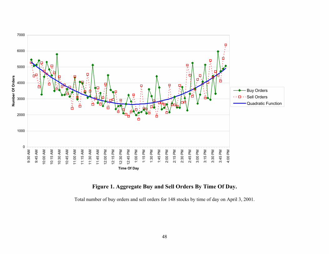
48

0

1000

2000

3000

4000

5000

6000

7000

9:30

AM

9:45

AM

10:0

0 AM

10:1

5 AM

10:3

0 AM

10:4

5 AM

11:0

0 AM

11:1

5 AM

11:3

0 AM

11:4

5 AM

12:0

0 PM

12:1

5 PM

12:3

0 PM

12:4

5 PM

1:00

PM

1:15

PM

1:30

PM

1:45

PM

2:00

PM

2:15

PM

2:30

PM

2:45

PM

3:00

PM

3:15

PM

3:30

PM

3:45

PM

4:00

PM

Time Of Day

Num

ber O

f Ord

ers

Buy OrdersSell OrdersQuadratic Function

Figure 1. Aggregate Buy and Sell Orders By Time Of Day.

Total number of buy orders and sell orders for 148 stocks by time of day on April 3, 2001.