a comparison of supervised learning algorithms
TRANSCRIPT

A Comparison of Supervised Learning Algorithms
Chapman Siu,
January 30, 2015
Introduction
This paper will introduce two data sets both from UCI repository index.
Data Sets
Pima Indian Diabetes
The Pima Indian Diabetes is a useful dataset to examine the health conditions which may be leading
indicators about how susceptible one is to diabetes in the future. I have used the full data set available
on the UCI repository [1] with the appropriate format changes to assist to analysis in R as outlined in the
mlbench package [2]. Besides the response variable being diabetes, all other variables are numeric
variables.
Wine Quality
The Wine Quality dataset used in this analysis is a subset of the Wine Quality dataset available from the
UCI repository index [3]. Here we examine a subset of the data set containing only red wines with scores
5, 6, or 7 and attempt to construct a classifier those wines. This is due to the scores below 5 and above 7
being outliers and white wines have different variables and hence would be a different classification
problem. Besides the response variable being categorical data, all other variables are numeric variables.
Comparisons between Pima Indian Diabetes and Wine Quality
Almost all variables in the Pima Indian Diabetes data set are positive correlated with each other, with
only a few variables only slightly negatively correlated.
Through research we can in fact determine that some variables (for example, insulin and glucose in Pima
Diabetes data set and “free sulfur dioxide”, “total sulfur dioxide”) are interdependent on each other.
This creates an interesting problem from the perspective of Machine Learning, since we would be able
to examine how well the various models perform (when applied naively) given these interdependent

variables. We attempted to correct these issues through the use of principal component analysis for
preprocessing the datasets.
Figure 1. The correlation matrix of the two data sets. Pima Indian Diabetes data set is on the left and Wine Quality data set is on the right. Many variables in the Pima Indian Diabetes are positively correlated with each other.
Beyond correlation structure the differences in the datasets could be expressed in terms of dimensions
and number of features. These would have an impact on the training times and complexity of the
resulting models.
Data Set Number of Rows Number of Features
Pima Indian Diabetes 768 8
Wine Quality 1518 11
Methodology
To accomplish all the algorithms the R programming language was used. The two required packages
required (along with their suggested packages and dependencies) are ‘caret’ and ‘mlbench’. Plots were
generated using ‘ggplot2’, ‘reshape’, reshape2’, ‘dplyr’, ‘plyr’, ‘gridExtra’, ‘lattice’, ‘corrplot’. Further
information is available in README.
Learning Algorithms
The training and test data set were created through stratified sampling on the response variable. 70% of
the data was used for the training set, whilst the remaining was used for the test set. Then all
algorithms were run with 3 repeats of a 10 fold cross validation on the training data set, with tuning
parameter grid with six levels, with manual tuning when required.
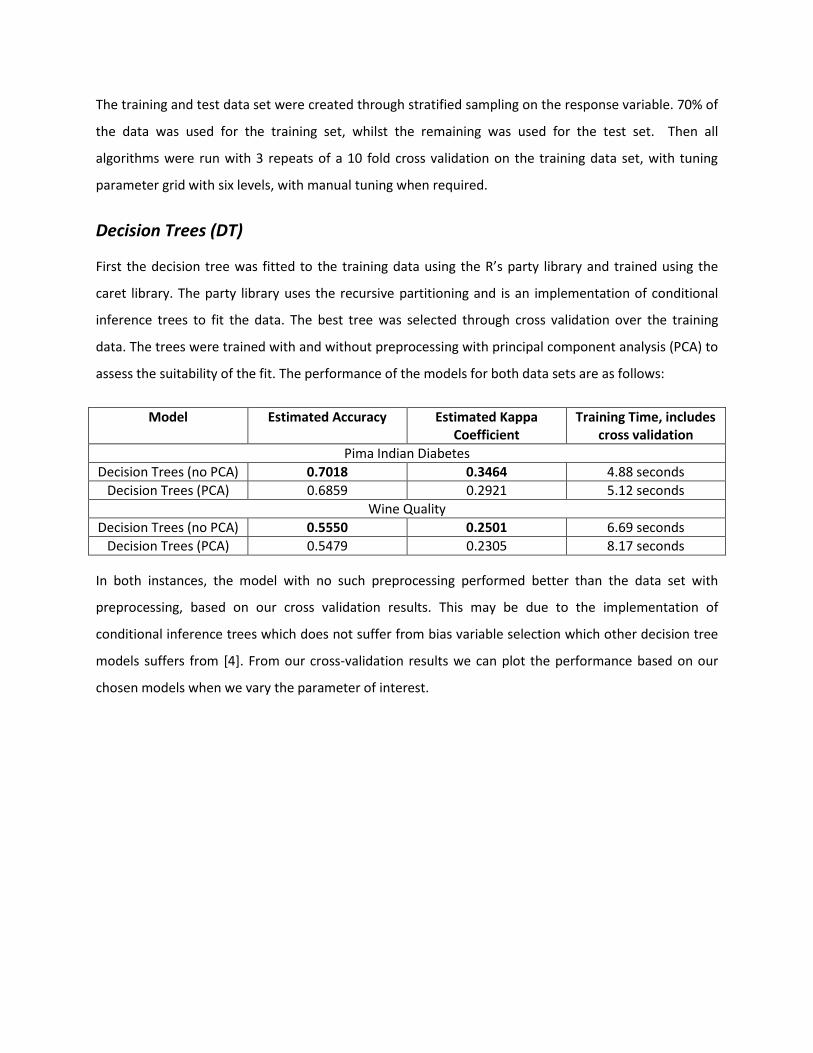
Decision Trees (DT)
First the decision tree was fitted to the training data using the R’s party library and trained using the
caret library. The party library uses the recursive partitioning and is an implementation of conditional
inference trees to fit the data. The best tree was selected through cross validation over the training
data. The trees were trained with and without preprocessing with principal component analysis (PCA) to
assess the suitability of the fit. The performance of the models for both data sets are as follows:
Model Estimated Accuracy Estimated Kappa Coefficient
Training Time, includes cross validation
Pima Indian Diabetes
Decision Trees (no PCA) 0.7018 0.3464 4.88 seconds
Decision Trees (PCA) 0.6859 0.2921 5.12 seconds
Wine Quality
Decision Trees (no PCA) 0.5550 0.2501 6.69 seconds
Decision Trees (PCA) 0.5479 0.2305 8.17 seconds
In both instances, the model with no such preprocessing performed better than the data set with
preprocessing, based on our cross validation results. This may be due to the implementation of
conditional inference trees which does not suffer from bias variable selection which other decision tree
models suffers from [4]. From our cross-validation results we can plot the performance based on our
chosen models when we vary the parameter of interest.

Figure 2. Estimated Accuracy under training for different parameters. On the left is the Pima Indian Diabetes and on the right is the Wine Quality data set
When we compare the two graphs, we can see that more aggressive “pruning” (setting a lower p-value
threshold) has a large impact on the estimated accuracy in Pima Indian Diabetes compared with Wine
Quality, which basically grew the largest tree possible. This conforms to our expectation of high
interdependence of the variables in the Pima Indian Diabetes compared with the Wine Quality data set.
Neural Networks (NNET)
Neural networks were fitted to the training data using the nnet package and trained using caret
package. The best neural network was chosen based on the accuracy from cross validation. Again,
models examining the effects of preprocessing through PCA were used to determine the optimal neural
network. In this scenario, preprocessing had a large impact on the fit for the neural network.
Model Estimated Accuracy Estimated Kappa Coefficient
Training Time
Pima Indian Diabetes
Neural Network (no PCA) 0.6627 0.2052 1:03 minutes
Neural Network (PCA) 0.7435 0.3957 49.58 seconds
Wine Quality
Neural Network (no PCA) 0.5734 0.2595 2:04 minutes
Neural Network (PCA) 0.5859 0.3023 1:44 minutes

The large performance improvement for neural networks in the Pima Indian Diabetes data set was most
likely due to the presence of correlated variables in the Pima Indian Diabetes set. Due to the nature of
the algorithm in Neural Networks it makes it difficult to split it otherwise.
In contrast, there was not a huge difference in the Wine quality data set whether or not we ran PCA on
the data first. This is probably due to the NNET model being more tolerant to interdependent variables
compared to DT model [5].
Also of interest is the change in the training time of the two data sets. With similar algorithms
implementing t he training time between the two data sets are by over a factor of three. This could be
due to variety of reason from Wine Quality having a data set roughly double the size of Pima Indian
Diabetes, having additional features or having a more complex response variable.
From our cross validation results we can plot the accuracy of our training results with the parameters of
interest; namely being number of hidden units and the weight decay. From here we can pick the
strongest performing model by the accuracy from repeated cross-validation.
Figure 3. Estimated Metrics based on varying the hyper parameters. On the left is Pima Indian Diabetes and on the right is the Wine Quality data set.
Boosting (BOOST)
Boosting was completed using the caret in conjunction with the gbm library in R. The implementation in
R's gbm library used was LogitBoost which classifies binary data and multinomial data.

Model Estimated Accuracy Estimated Kappa Coefficient
Training Time, including cross validation
Pima Indian Diabetes
LogitBoost (no PCA) 0.7270 0.3831 6.15 seconds
LogitBoost (PCA) 0.7135 0.3398 5.75 seconds
Wine Quality
Multinomial LogitBoost (no PCA)
0.5825 0.2936 41.02 seconds
Multinomial LogitBoost (PCA)
0.5685 0.2740 37.19 seconds
The reduction of performance under PCA is in line with [5], demonstrating that boosting algorithms are
generally robust against independent variables.
Furthermore, it is interesting to notice the change in the speed of the algorithm across the two data
sets. Although in both cases, the algorithm completed very quickly, the wine quality data set took
roughly seven times longer to determine the optimal algorithm compared with the Pima Indian Diabetes
data set. The results of cross validation can be plotted and observed below
Figure 4. Estimated Accuracy based on varying the hyperparameters. On the left is the results from the Pima Indian Diabetes, and right is the Wine Quality data set.
Support Vector Machines (SVM)
Support vector machines using the Gaussian Radial basis function was the support vector machine of
choice. This was implemented using the kernlab library and again trained using the caret library. Linear

kernels were not tested since it has been shown that these are a special case of the Radial Basis
Function. A summary of the training results for SVM are below:
Model Estimated Accuracy Estimated Kappa Coefficient
Training Time, including cross
validation
Pima Indian Diabetes
SVM (no PCA) 0.7377 0.3750 16.44 seconds
SVM (PCA) 0.7352 0.3704 19.58 seconds
Wine Quality
SVM (no PCA) 0.5921 0.2901 38.44 seconds
SVM (PCA) 0.5894 0.2963 39.79 seconds
We can see that in both models, the algorithms performed better with no preprocessing through PCA,
this would be in line with the expectation that SVM model has high tolerance to irrelevant attributes [5].
With this knowledge we can plot the cross validation results over the parameters used for SVM with the
Gaussian Radial Basis function.
When comparing the performance difference when using the SVM models, although the training on
both data sets were relatively quick, the time taken on the Wine Quality data set was still double the
amount of time taken for the Pima Indian Diabetes data set.
Figure 5. The estimated metrics based on varying the hyperparameters. On the left is the Pima Indian Diabetes, and on the right is the Wine Quality data set.
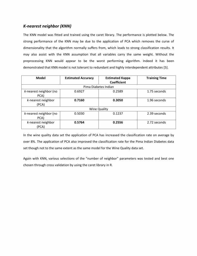
K-nearest neighbor (KNN)
The KNN model was fitted and trained using the caret library. The performance is plotted below. The
strong performance of the KNN may be due to the application of PCA which removes the curse of
dimensionality that the algorithm normally suffers from, which leads to strong classification results. It
may also assist with the KNN assumption that all variables carry the same weight. Without the
preprocessing KNN would appear to be the worst performing algorithm. Indeed it has been
demonstrated that KNN model is not tolerant to redundant and highly interdependent attributes [5].
Model Estimated Accuracy Estimated Kappa Coefficient
Training Time
Pima Diabetes Indian
k-nearest neighbor (no PCA)
0.6927 0.2589 1.75 seconds
k-nearest neighbor (PCA)
0.7160 0.3050 1.96 seconds
Wine Quality
k-nearest neighbor (no PCA)
0.5030 0.1237 2.39 seconds
k-nearest neighbor (PCA)
0.5764 0.2556 2.72 seconds
In the wine quality data set the application of PCA has increased the classification rate on average by
over 8%. The application of PCA also improved the classification rate for the Pima Indian Diabetes data
set though not to the same extent as the same model for the Wine Quality data set.
Again with KNN, various selections of the “number of neighbor” parameters was tested and best one
chosen through cross validation by using the caret library in R.

Figure 6. The estimated metrics based on varying the hyperparameters. On the left is the Pima Indian Diabetes and on the right is the Wine Quality data set.
Performance Metrics
In general for these sample data sets each algorithm performs reasonably well and similar to each other.
I have purposely chosen two data sets where one has binary response variable (Pima Indian) and the
other had an ordered factor as the response variable (Wine Quality).
Overall Performance
The table and plot below shows the estimated accuracy and kappa coefficient, calculated through
resample, and the estimated accuracy based on the hold-out test set. The best performing model for
each metric is boldfaced , whilst the worse performing model for each metric is italic.
Training set Training set Hold-out Test set
Model Estimated Accuracy (mean)
Estimated Kappa (mean)
Estimated Accuracy (mean)
Pima Indian Diabetes
DT 0.7018 0.3464 0.7609
NNET 0.7435 0.3957 0.7696
BOOST 0.7280 0.3798 0.7565
SVM 0.7352 0.3704 0.7826
KNN 0.7160 0.3050 0.7739
Wine Quality
DT 0.5550 0.2501 0.6523
NNET 0.5859 0.3023 0.6974
BOOST 0.5825 0.2936 0.6955

SVM 0.5921 0.2901 0.7073
KNN 0.5764 0.2556 0.6287
Figure 7. On the top row is the accuracy metric based on the test data, in the middle and last row is the estimated accuracy and kappa coefficient based on the training data respectively. Models are sorted on test data accuracy.
The top row of Diagram one shows the 90% and 95% confidence interval for Accuracy (in blue and red
respectively) for the hold-out test set based on binomial test against the null hypothesis that the entries
were classified at random. The next two rows show the box plot of Accuracy and Kappa coefficient
respectively based on resampling the training data. The models for each one are ranked according to the
accuracy of the test data. Of particular interest is the spread of the resample results in the training set.
This data shows the potential spread of performance for each model through resampling.
The model with the greatest variation in performance was KNN; performing well on the Pima Indian
Diabetes, but poorly on the wine quality data set. This reflects the nature of KNN which requires strong

domain knowledge to understand the appropriate distance metric in order to perform well. Based on
this, it would suggest that the out-of-box performance for KNN was suitable for Pima Indian Diabetes,
but not suitable for Wine Quality data set. This is most likely related to the correlation structure of the
data set, since all variables were positively correlated with each other, which lead to the nearest
neighbor model working well since all variables were correlated with each other.
The strong performance for NNET in the Pima Indian Diabetes data set based on the training data
suggests that NNET model was overfitted, since the test results did not reflect the performance seen in
the training data. In comparison, for the Wine quality data set, the NNET model did not appear to have
this issue, performing roughly the same compared with the other models in consideration.
The difference in the BOOST model performance might be attributed to the different implementations
used for classifying binary versus classifying three categories. As such, there is not enough information
to determine whether this was a fair comparison of BOOST models. Regardless, we can observe on the
whole, the estimated model accuracy is fairly stable, having a small range of values indicated by the box
plot. This may also be a reflection of the poor performance BOOST models have with data sets that are
highly correlated.
Model Training Time Considerations
Different models clearly have different training times. Unsurprisingly models with more hyper-
parameters took longer to train. Since training in general takes place using a grid search the increase of
training time is not unexpected. The nature of the algorithm also had a large impact on the training
time.
Number of records and features in the training set also had a large impact on the training times of the
various models. Training times more than doubled for NNET, BOOST, SVM models and increased by
roughly 50% for DT and KNN, when we trained between the two datasets. We may infer that training
times of NNET, BOOST, SVM may increase at a faster rate than the size of a data set. This is most likely
due to two reasons:
the iterative nature of the models
each model possessing multiple parameters

Since grid search is used to optimize the parameters, the increase in number of records and features
would only compound the training time required to determine the optimal parameters. The training
time for KNN was also the quickest due to the nature of it being a lazy learner. The time required to
determine the predictions were not included since they were insignificant due to the size of the data
sets.
Conclusion
On a practical level the best model based on the these two data sets and applying machine learning
algorithms naively would be SVM. It performed well in the training set data and also in the test set. The
spread of results as indicated in the resampled estimations of Accuracy and Kappa coefficient reveals
narrow spread of results ensuring consistency when classifying data.
Perhaps one area which should be examined is the impact that domain knowledge has on the
classification results, rather than naively applying supervised learning algorithms. Due to this approach it
is perhaps not too surprising that SVM models performs well, since with a suitable choice of parameters
for a kernel an SVM can separate any consistent data set [6]. Furthermore, through the firm statistical
foundations that SVM are built on, SVM will search for a regularized hypothesis that fits the available
data well without over-fitting [6].
References [1] https://archive.ics.uci.edu/ml/datasets/Pima+Indians+Diabetes
[2] http://cran.r-project.org/web/packages/mlbench/mlbench.pdf
[3] https://archive.ics.uci.edu/ml/datasets/Wine+Quality
[4] T. Hothorn, K. Hornik and A. Zeileis. Unbiased Recursive Partitioning: A Conditional Inference
Framework. Available from: http://statmath.wu-wien.ac.at/~zeileis/papers/Hothorn+Hornik+Zeileis-
2006.pdf
[5] S.B. Kotsiantis. Supervised Machine Learning: A Review of Classification Techniques. Available from:
http://link.springer.com/article/10.1007%2Fs10462-007-9052-3
[6] R. Burbidge, B. Buxton. An Introduction to Support Vector Machines for Data Mining. Available from:
http://www.svms.org/tutorials/BurbidgeBuxton2001.pdf