a climatology-based qc procedure for argo oxygen...
TRANSCRIPT

A climatology-based QC procedure for Argo oxygen data
• Hugh Doyle (ACE/CSIRO), Esmee Van Wijk (CSIRO), Luke Wallace (CSIRO), Tom Trull (ACE/CSIRO)

Argo oxygen data A large number of oxygen measurements have been made by Argo profiling floats, and will continue to be made at an increasing rate.
Over 450 floats have been deployed with oxygen sensors - the CSIRO has deployed 60 such floats.
Unlike temperature, salinity, and pressure data, strict QC procedures have yet to be agreed upon and implemented for dissolved oxygen by Argo data centres.

Argo oxygen data Studies have shown that oxygen sensors produce highly stable data over months to years i.e. minimal sensor drift of order 1 % per year [Körtzinger et al., 2005; Tengberg et al., 2006; Riser and Johnson, 2008; Riser and Johnson, 2015].
However, large discrepancies have been documented (up to 30%) between profiling floats and discrete water samples taken nearby the float [Kobayashi et al., 2006; Takeshita et al., 2013].
Clearly there is a need to QC the Argo oxygen data set.

Argo oxygen data Takeshita et al., (2013) have suggested a QC procedure for oxygen data based on comparison of data to a monthly climatology, which therefore drives corrected oxygen data toward the climatology.
We have implemented and evaluated this approach by comparison of the CSIRO Argo oxygen data set to the climatology CARS 2009.

CARS 2009 CARS 2009 is a monthly climatology for temperature, salinity, [O2] (µM), and oxygen percent saturation (%Sat = [O2] / [O2Sat] x 100), where [O2Sat] is the oxygen saturation at solubility equilibrium [Garcia and Gordon, 1992].
All oxygen measurements used to create the climatology were made by Winkler titration.
The standard uncertainty of the climatology for the majority of the open ocean is estimated to be ~ 2 %Sat [Garcia et al., 2010].

Oxygen sensors CSIRO floats that measure oxygen are equipped with either a Sea-Bird SBE43 Electrode, Sea-Bird SBE63 Optode or an Aanderaa AA3830 Optode.
The SBE43 is a Clark-type electrode, where O2 diffuses across a membrane and is converted to OH- at a gold cathode. The [O2] is proportional to the induced current [Edwards et al., 2010].
The Optodes are based on dynamic luminescence quenching, where the luminescence lifetime of a luminophore is quenched in the presence of O2. The luminophore responds to the partial pressure of O2 [Tengberg et al., 2006].

Sensor failure Before comparison of sensor data to the climatology, oxygen data was qualitatively assessed for unreasonable cycles and apparent sensor failures.
The most common symptoms were negative [O2], or entire profiles where [O2] = 0 µM.
In cases where the sensor failed middeployment, data until then was used.
Sensor failure was far more common in our data set for SBE43 electrodes than Aanderaa or SBE63 Optodes.

Oxygen correction coefficients Float specific oxygen dependent correction terms were determined by performing a model II linear regression on %Satfloat versus %SatCARS using two different approaches:
%SatCARS = C0,%Sat + C1,%Sat x %Satfloat (1)
%SatCARS = C1,%Sat x %Satfloat (2)
where C0 (offset) and C1 (gain) are the coefficients from the regression.

Oxygen correction coefficients The corrected float oxygen data, %Satfloat
*, is therefore calculated using one of the two different approaches:
%Satfloat* = C0,%Sat + C1,%Sat x %Satfloat (1)
%Satfloat* = C1,%Sat x %Satfloat (2)
The standard deviations (SD) of the coefficients are noted and used as a QC.

An example
Figure shows cycle positions of the float 5901644. The colour scale represents the age of the float. The first profile is in dark blue while the last profile is in dark red.

An example
Time series plot of dissolved oxygen obtained from the Argo float. The grey line shows the mixed layer depth - as calculated using a density criterion of 0.03 kg/m3 (Montegut et al., 2004).

An example
Figure shows oxygen profiles (%Sat) from float in blue and corresponding CARS 2009 data in red. The vertical structures seem to match relatively well throughout the water column. However, the float data is systematically lower than the climatology.

An example
Figure shows CARS 2009 oxygen data plotted as a function of the corresponding float data. This plot is used to calculate C1 (gain) and/or C0 (offset) for a float. The red line is the 1:1 line.

An example
Not all data is used to obtain correction coefficients. The data used and omitted are represented by black circles and open blue circles, respectively. The green line is the model II linear regression.

An example
Oxygen measurements taken in strong vertical gradients are omitted from the regression in order to minimize bias due to errors, such as slow sensor response time. We have chosen to restrict the data to measurements made in the mixed layer and below 1500 db.

An example
A seasonal filter has also been applied to the mixed layer, i.e. only data collected from May through September is used. This approach provides a better comparison to the climatology as the %Sat remains very close to solubility equilibrium over these months.
An example
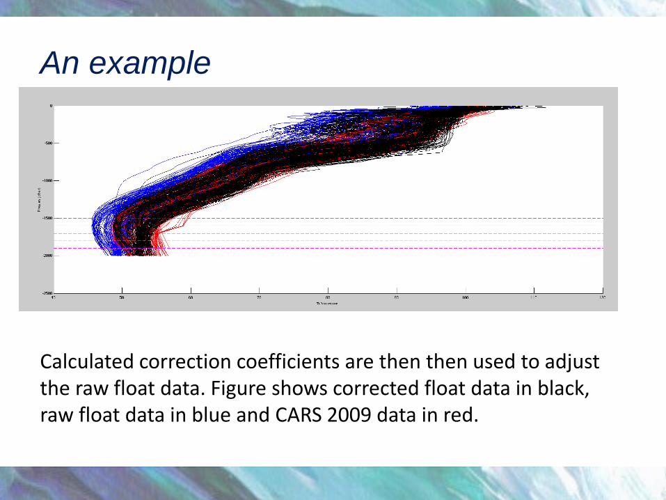
Calculated correction coefficients are then then used to adjust the raw float data. Figure shows corrected float data in black, raw float data in blue and CARS 2009 data in red.

An example
The MATLAB GUI that has been developed allows us to assess the correction in the mixed layer (top panel), and at specified positions in the water column (bottom panel = 1900 db). It also allows temporal drift to be evaluated on a case by case basis.

Calibration validation
In order to verify the climatology-based QC procedure we compared corrected float data to calibrated oxygen profiles taken on deployment of several floats.

Calibration validation
Figure on left: Calibrated oxygen profiles (%Sat) collected at the float deployment. Figure on right: Difference between calibrated data and CARS 2009 at the profile position.
0
200
400
600
800
1000
1200
1400
1600
1800
2000
0 20 40 60 80 100 120
Dept
h (d
b)
%Sat (CTD)
0
200
400
600
800
1000
1200
1400
1600
1800
2000
-20 -10 0 10 20
Dept
h (d
b)
∆%Sat (CTD - CARS)

Calibration validation
On average the calibrated profiles and the climatology agree well at the surface (~3 %Sat) and in the deep (~1 %Sat).
The poor agreement in the midwater column is most likely due to water masses not accurately captured by the climatology.
0
200
400
600
800
1000
1200
1400
1600
1800
2000
0 20 40 60 80 100 120
Dept
h (d
b)
%Sat (CTD)
0
200
400
600
800
1000
1200
1400
1600
1800
2000
-20 -10 0 10 20
Dept
h (d
b)
∆%Sat (CTD - CARS)

Calibration validation Figure shows difference between calibrated data and raw float oxygen data. The average agreement at the surface and in the deep is 8 and 6 %Sat, respectively.
0
200
400
600
800
1000
1200
1400
1600
1800
2000
-20 -10 0 10 20
Dept
h (d
b)
∆%Sat (CTD - Argo)

Calibration validation
Figure shows difference between calibrated data and data corrected using C0 (offset) and C1 (gain). The average agreement at the surface and in the deep is 2 %Sat.
0
200
400
600
800
1000
1200
1400
1600
1800
2000
-20 -10 0 10 20
Dept
h (d
b)
∆%Sat (CTD - Argo'')

Calibration validation Figure shows difference between calibrated data and data corrected using C1 (gain) only. The average agreement at the surface and in the deep is 2 %Sat.
0
200
400
600
800
1000
1200
1400
1600
1800
2000
-20 -10 0 10 20
Dept
h (d
b)
∆%Sat (CTD - Argo')
Conclusions The correction algorithm with C0 (offset) and C1 (gain) terms (as proposed by Takeshita et al., (2013)), offers no significant benefit over simply adjusting C1 (gain) while forcing the offset to 0. [This is consistent with laboratory optode studies that suggest gain variations are the primary mode of sensor bias. Additionally we found that climatology based drift correction was uncertain and unwarranted, consistent with recent work from Riser et al (2015) ]
The mean (±1σ) C1 (gain) calculated for all CSIRO floats (n = 60) was 1.06 ± 0.04. Corrected data for these floats is likely to be available via ARGO GDACS by end 2015.
The average correction inferred using this climatology-based procedure for the global Argo oxygen data set is ~20% (Takeshita et al., 2013).

Conclusions Cons: Method is prone to errors in areas where deep oxygen is subject to short-term variability, such as frontal zones and the subpolar North Atlantic (Stendardo and Gruber, 2012).
The climatology is limited over large regions of the ocean leading to increased uncertainty in the corrections.
This method only corrects for calibration errors. It does not correct for dynamic errors, such as slow sensor response.

Conclusions Pro:
A climatology-based correction provides a post-deployment QC protocol for all floats.
The vast majority of oxygen floats have been deployed without stringent calibrations or corresponding hydrographic casts, and this approach is currently the only path to a consistent dataset. In future, this situation is likely to improve, as calibration protocols using air O2 measurements are incorporated. Nonetheless, comparison to climatologies will remain essential.

SCOR WORKING GROUP 142
Feb. 2014 meeting, identifies measurement of air O2 as an effective sensor calibration to mitigate poor factory calibration. • Analysis of 24 UW/MBARI floats shows O2 bias in mixed layer reduced from 30 µmol/kg to 2 µmol/kg vs. Winkler. • ADMT-15 encourages WG 142 to provide expert recommendation to manufacturers. • Argo Canada (D. Gilbert) reports their O2 floats all made air oxygen measurements, possibly all Apex O2 floats did. • WG 142 agrees at Brest to write recommendation to manufacturers that all floats should make air O2 measurements (SBE 63 before deployment if not during deployment). Should have minimal impact on float ops.