3D Modeling of Interference Within Microwave Transmission Corridors

By: Larry T. Nierth, GISP & Daniel C. Bally, AICP, GISP

Abstract: The City of Houston has proposed the construction of fifty-four new microwave transmission towers to enhance emergency response efforts. The GIS Division was asked by the Information and Technology Department to develop a method for modeling and visualizing the proposed microwave transmission corridors in order to locate any possible obstructions to the transmission signals. Using LIDAR and transmission corridor elevation models, a sophisticated process was developed to identify existing obstructions, indicate future building height restrictions, and to efficiently illustrate the impacts of different planning scenarios. This presentation is directed at those who may be asked to undertake a similar project for modeling spatial networks in a 3D environment, and would like to see an example of progress from conception through completion. The discussion will explain the project's design, the variety of geoprocessing and visualization methods used, the results, and their implication in the planning process.

1

Introduction: The City of Houston’s Information Technology Department needed to locate and visualize potential signal obstructions between proposed microwave transmission sites across the city. The City’s GIS Technology Division of the Planning and Development Department was asked to develop a process that allows for the timely and efficient identification of possible obstructions without the need of sending a surveying crew to the proposed locations to physically verify probable signal impediments. Procedures: Many steps were needed to complete the task, and it required use of several software packages. Below are the steps followed to take a spreadsheet containing X, Y, and Z coordinates all the way to a finished 3D model.

• Format Excel spreadsheets with coordinate and elevation data • Create AutoCAD scripts from Excel spreadsheets to automate transmission corridor creation • Create and covert CAD files for use in GIS analysis

o .DWG Polyline Feature Class TIN Raster • Acquire and process full-feature LIDAR data

o .LAS MultiPoint Feature Class TIN Raster • Raster calculations to determine obstructions

Excel

The initial data delivery received from the IT department was simply an Excel file containing the proposed locations of dozens of microwave antennae. The data included the latitude, longitude, and elevation above ground level for each transmitter and receiver with an indication of which location was the beginning or ending point for the transmission corridor. A fair amount of data manipulation occurred to translate the initial spreadsheet into a format that was more compatible with AutoCAD scripting process. These changes included reformatting the spatial coordinates from Degrees-Minutes-Seconds to NAD 1983 State Plane Texas South Central (ft.) and adding ground elevation derived from a digital elevation model created from 2 ft. contours provided by the Harris County Flood Control District to the proposed transmitter/receiver elevations to establish height above sea-level for each location. It was necessary to determine height above sea level as the LIDAR data used in subsequent steps provide elevations above sea level as well.

2

AutoCAD Automation Once the data was appropriately formatted in Excel another spreadsheet was created in the same workbook to construct an AutoCAD script for each individual corridor in order to automate the creation of the microwave transmission network. AutoCAD 2010 or newer in necessary as the new Mesh modeling functionality is critical to establishing interoperability between CAD and GIS software. Each corridor’s script, such as that in Figure 1, was appended to a larger AutoCAD script file (.scr) so that the entire network could be created in AutoCAD at one time, as partially shown in Figure 2. The resultant file was saved as an AutoCAD version 2004 .dwg. Saving the resulting file as a version 2010 .dwg created incompatibilities with ArcGIS. ; ; AUTOMATED SCRIPT TO CREATE MESH CYLINDERS ; -layer M Lake_Houston_AT_Bohemian_(Rawe_#310231) ; first 3d point point 3189357.28847,13899587.6716,183.14319992 ; second 3d point point 3227604.35057,13907953.6467,180.64665985 ; start Mesh mesh ; create Cylinder CY ; starting @ first 3d point 3189357.28847,13899587.6716,183.14319992 ; with a radius of 50 ; end point is Axis A ; of second point 3227604.35057,13907953.6467,180.64665985 ; explode explode ALL

Figure 1 - Example of AutoCAD script syntax created within Excel

Figure 2 - A view of the resulting transmission corridor network.

CAD & GIS Interoperability

3

Due to the inherent interoperability functionality of ArcGIS, the resulting AutoCAD file was immediately viewable and useable. The point, polyline, polygon, and multipatch features of the CAD file are compatible with GIS. Figure 3 illustrates the native CAD file in ArcScene. For analysis, the Polyline features were critical. For visualization, the Polygons are useful.

Figure 3 - A similar view of the microwave transmission network .dwg in ArcScene

GIS Analysis Two parallel paths were followed in GIS during the analysis phase of this project. The first involved the processing of full featured LIDAR to gather elevation data within a certain distance of the transmission corridors. The second path involved processing the elevation data from the corridors themselves. Ultimately, possible obstructions to the microwave transmission corridor network were determined by finding areas where the LIDAR elevation is greater than the corridor elevation.

4

Figure 4 - Full feature LIDAR elevation raster

The LIDAR data was initially processed using a 3rd party extension for ArcMap called LP360 by QCoherent (http://www.qcoherent.com/product.html). This extension quickly and efficiently handles and processes native LIDAR .las files and was an integral part of this project. Without full feature LIDAR elevation data it would have been impossible to determine obstructions to the transmission corridor network. The general process for the LIDAR data was to convert .las data to MultiPoint feature class, create a TIN from that feature class, and then create a raster from the TIN. This was done to preserve the integrity of the elevation data and to have a data format that lent itself to analysis through raster calculations. The raster, as shown in Figure 4, is ultimately what is employed in the obstruction calculation analysis. Model Builder was utilized in the initial planning stages and a more thorough Python script was developed from the Model Builder framework to automate the LIDAR MultiPoint TIN Raster processing.

5

Figure 5 - Microwave transmission corridor and full feature LIDAR elevation rasters.

Similar to the LIDAR processing, each corridor went through a multistage transformation process. The polyline feature of the CAD file was exported into a file geodatabase. This initial polyline feature class contained the corridors for the entire network. Individual corridors were then created from the larger feature class to expedite processing. Each corridor was converted from a Polyline to a TIN, and that TIN was converted into a Raster. Figure 5 illustrates the resulting corridor raster. The gradient from left to right indicates an overall slope to the corridor. The subtle gradient from top to bottom indicates the elevation changes of the corridor due to its cylindrical nature.

6

Figure 6 - Obstructions determined by areas where the LIDAR elevation is greater than the corridor elevation.

With both the full feature LIDAR elevation and microwave transmission corridor elevation data processed and converted to rasters, it was simply a matter of subtracting the LIDAR elevation from the corridor elevation to determine areas where the full feature data could obstruct the proposed corridor. The results for one corridor are shown in red in Figure 6. It should be noted that two microwave transmission corridor networks were created in AutoCAD. One network was created with full 360° cylinders for visualization purposes, and the other was created with the180° lower half-cylinders for analysis. Using half-cylinders was another critical component to the success of this project. Creating a TIN that would be converted to a raster from a full cylinder would have misrepresented the elevation data during the raster calculations because of the overlapping vertical elevations.

7

3D Visualization:

Figure 7 – 3D scene looking to the northwest of a building obstruction.

There were many options for visualizing obstructions to the microwave’s path, once the microwave cylinder rasters were subtracted from the full feature LIDAR rasters, and the obstruction locations were known. GIS provides the ability to examine all of the individual microwave shots and show what is encroaching into the microwave transmission and to what extent. Volumes and areas for each obstruction can be calculated to determine if changes need to be made to minimize the impact to signal degradation. Buildings that were found to be an obstruction were especially intersecting because unlike utility pylons and other towers or power lines, a building has the ability to completely block a signal from reaching the antenna. In Figure 7 and Figure 8, an upper edge of a building (in the full feature LIDAR TIN data) is shown intersecting the microwave cylinder hovering above it.

Figure 8 - 3D scene looking to the southeast of a building obstruction.

8

Another option was to align the viewing angle straight down the center of the microwave transmission and view the obstruction heights in relation to the full microwave cylinder walls.

Figure 9 - Another option was to align the viewing angle straight down the center of the microwave transmission

and view the obstruction heights in relation to the full microwave cylinder walls.

Graphics like Figure 9 make invisible concepts visible by colorizing the actual transmission corridor cylinder and showing what is inside along with actual elevation values. In order to visualize microwave corridors as horizontal cylinders (having different elevations at their endpoints), many steps had to be performed. The interpolate line tool (in 3D Analyst) works well to construct 3D lines that start and end at differing elevations for each microwave corridor. Below is a summary of how the visualizations were achieved.

9

• AutoCAD 2010 mesh functionality was utilized to generate what would be considered a 3D radial buffer along each corridor’s interpolated 3D centerline (mentioned above). These polygons (or their multipatch counterparts) can be rendered and modeled in ArcScene with the LIDAR and tower location data.

• Then, a color ramp was assigned to the 3D polygon based on elevation values, and it was made partially transparent to see any areas where the full feature LIDAR TIN protruded through the transmission corridor.

• Selections were made for all actual LIDAR points that were inside the obstructions, and they were displayed as well to provide exact spot elevations along the TIN surface.

• Depending on the viewing angle and the amount of obstruction visible, a half cylinder was used in lieu of a full cylinder.

• The final models along with all final graphics were rendered in ArcScene. The volumetric information was calculated by first identifying and isolating the section of the microwave cylinder were an obstruction occurred, and using the cylindrical volume formula to attain its volume in square feet. The Tin Polygon Volume tool (in 3D Analyst) was used to isolate and calculate the volume of the portion of the full feature LIDAR TIN that was inside the cylinder. This was the volume of the obstruction itself. For the example shown in Figure 10 a percentage of 7.72% was calculated as the final volume of the obstruction for that portion of the microwave corridor.

Figure 10 – Volumetric calculations for the obstructed area.

Area calculations are a little more complex. A signal can (theoretically) travel almost all the way though the corridor, only to be blocked at a single location within the pipe. Area fluctuates along the obstruction depending upon where you are located and how far into the cylinder the obstruction protrudes at that exact point. Figure 11 below shows two paths through the cylinder that were unobstructed, while the other three paths were blocked.

10

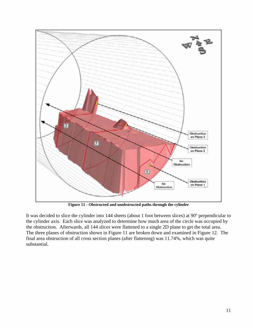
Figure 11 - Obstructed and unobstructed paths through the cylinder

It was decided to slice the cylinder into 144 sheets (about 1 foot between slices) at 90º perpendicular to the cylinder axis. Each slice was analyzed to determine how much area of the circle was occupied by the obstruction. Afterwards, all 144 slices were flattened to a single 2D plane to get the total area. The three planes of obstruction shown in Figure 11 are broken down and examined in Figure 12. The final area obstruction of all cross section planes (after flattening) was 11.74%, which was quite substantial.

11

Figure 12 - Area analysis of sample obstruction slices.

12

Results and Impacts: The City of Houston saves close to $100,000 in tax payer dollars for every obstruction that is caught and fixed without having to send a crew out and check for signal loss. Finding and fixing potential problems utilizing the City’s GIS data also can save potentially thousands of dollars in the design phase involving new legs of the microwave transmission network as well. Several options exist for correcting the obstructions including the following:

1) Elevate or lower the microwave antennas to clear the obstruction. 2) Relocate the tower upon which the microwave antennas are located to another position

inside the same parcels. 3) Relocate the tower upon which the microwave antennas are located to different parcels

altogether.

June 3, 2010

13