123 5 rock mechanics this chapter describes the rock - posiva

123

5 ROCK MECHANICS This chapter describes the Rock Mechanics Descriptive Modelling. The modelling uses the characterisation data listed in Section 2.3 and the resulting rock mechanics model will then be used for predicting the impact of ONKALO construction, as described in Section 7.3.

5.1 Conceptual Rock Mechanics Model and Its Component Parts

5.1.1 The rock mechanics conceptual model In a mechanics problem, the boundary conditions and geometry are specified, together with the material properties. A perturbation is then applied to the system in the form of changes to

• the boundary conditions,

• geometry, or

• material properties.

The consequences of the perturbation are then evaluated. When the material involved is rock, it is a rock mechanics problem, as illustrated in Figure 5-1. This is the conceptual model.

F1

F2F3

Fn

Discontinuities

Intact rock

Boundaryconditions

Excavation

Water flow

Figure 5-1 The conceptual rock mechanics model and its components.

For example, a change to the boundary conditions would involve alteration of the forces, Fi, illustrated in Figure 5-1. These force boundary conditions are usually expressed via the principal stresses, and so a change in the boundary conditions would involve a change in the far-field natural stress state. This is unlikely, except for the case of dynamic changes resulting from earthquakes.

A change in the geometry occurs, however, when an excavation is made, for example the excavation illustrated in Figure 5-1. Such an excavation could be the ramp of the ONKALO, a shaft, or the deposition tunnels and holes, and when an excavation is made, there are inevitable effects because:

• the stiffness of the rock in the tunnel volume has been reduced to zero,

124

• the stresses have been locally realigned to be parallel and perpendicular to the excavation surfaces, having passed along a stress path, and there have been changes also in magnitude,

• the hydraulic pressure in the tunnel has been reduced to atmospheric pressure.

In the immediate vicinity of the excavation (due to blasting and stress concentration), there is an excavation damaged zone, EDZ, in the sense that irreversible changes have occurred, e.g. the formation of microcracks. Further away from the excavation, there is an excavation disturbed zone, where the changes can be reversed, e.g. elastic displacements. A recent paper summarizes the EDZ effects in the context of radioactive waste disposal (Tsang et al. 2004).

A change in the material properties can occur as a result of excavation, e.g. damage (spalling) of rock around the excavation when the secondary stresses become too high. There can also be long-term (creep) effects, i.e. continuing displacement as a result of the application of a constant stress. Additionally and in the longer term, there can be changes to the rock fractures and brittle deformation zones as a result of groundwater flow, e.g. calcite precipitation in the fractures, which not only affects their hydraulic properties but also their fracture stiffness and strength.

5.1.2 The components of rock mechanics Given the subject matter described above and the illustration of the rock mechanics problem in Figure 5.1, the key components are as follows.

• The boundary conditions expressed as the pre-existing primary stresses in the rock mass.

• The unfractured intact rock

• The individual fractures

• The brittle deformation zones (the term brittle distinguishes these zones from, for example, shear zones, in which they may have been no brittle deformation)

• The operating rock mechanics mechanisms, e.g. elastic deformations, and the mechanisms which are coupled with other processes and interact with other disciplines, e.g. the changes in effective stress caused by changes in the hydraulic pressure

• The perturbations introduced by changes in boundary conditions, geometry and/or material properties

• Evaluating the effects of the perturbations

The salient points associated with these seven aspects of the conceptual model are briefly described in the following sub-sections.

125

5.1.3 The boundary conditions expressed as the pre-existing primary stresses in the rock mass.

The in situ rock stress state is expressed via the magnitudes and orientations of the three mutually orthogonal principal stresses. In Fennoscandia, the major principal stress tends to be horizontal and oriented NW-SE. However, the rock stress is affected by the geological conditions, especially the major lineaments and brittle deformation zones, which can locally affect the principal stress magnitudes and orientations. There could well be significant differences in the stress states between various sites. Thus, the stress state cannot be assumed: it has to be established through measurements.

5.1.4 The intact rock The key rock mechanics properties of the intact rock, i.e. the rock without visible fractures, are its stiffness and strength. The stiffness determines how much strain will occur as the result of stress changes induced by excavation, and the strength determines when damage/failure will occur as the result of the applied secondary stresses, particularly in the EDZ region.

Key aspects of the intact rock properties are whether the rock is inhomogeneous (having different properties in different locations) and/or anisotropic (having different properties in different directions). The inhomogeneity can be taken into account via changes in the lithology, but the anisotropy requires an understanding of the foliation. In certain directions, the stiffness and especially the strength will be a function of the applied stress relative to the orientation of the foliation.

5.1.5 The individual fractures This refers to the individual fractures within the rock mass, which are not part of the brittle deformation zones. Because the rock stress has been applied through geological history via the three principal stresses, these fractures tend to occur in certain preferred directions, i.e. to be clustered into sets.

There are many characteristics of fractures, of which the most important are their frequency, orientation, trace length, stiffness and strength.

5.1.6 The brittle deformation zones The brittle deformation zones are major zones of fracturing characterized by a large geometrical extent and a much greater width (in metres) than individual fractures (in millimetres). It is evident from Figure 5-1 that the brittle deformation zones will have a greater mechanical effect than an individual fracture.

5.1.7 The operating rock mechanics mechanisms The operating mechanisms are elasticity, fracture and flow and their interactions with other processes and changes.

• Elastic deformation occurs when the stresses are changed – but elastic deformation is fully recoverable; also, all the energy involved in elastic deformation is fully recoverable, by definition.

126

• Fracture occurs when the stresses are increased. Microcracking can in principle occur right from the onset of applying stress, but it is generally assumed that microcracking starts at about 40-50% of the compressive (peak) strength in crystalline rock.

• Flow refers to continuing displacement at constant stress. For example, the rock may initially crack around a tunnel as it is being excavated because of the increased stress, but it can also deform and crack further over time as the high stress is maintained.

• Mechanisms which are coupled with other processes and disciplines are alterations to the effective stress when the water pressure changes, and changes to fracture hydraulic conductivity when stress magnitudes change close to an excavation. The chemical erosion of fractures or the precipitation of minerals on fracture surfaces can also affect their mechanical properties.

5.1.8 The introduced perturbations The initial perturbation is the excavation itself. This is followed by the thermal load as a result of emplacement of the canisters.

5.1.9 Evaluating the effects of perturbations There are only two main ways of evaluating the effects of the engineered perturbations: empirical assessments and numerical modelling. Both should be used but, of the two, numerical modelling is preferred because of its flexibility and ability to predict conditions for a variety of circumstances. This is especially true for radioactive waste disposal where we do not have the precedent practice information, which is required to implement the empirical approaches.

5.2 Evaluation of information The rock mechanics data presented in Section 2.3 have been collected over a long time and many of these data have been analysed in various published studies (see Appendix 3). However, there has been some re-assessment of the data and this is discussed in Section 5.4.

5.2.1 Summary of the rock mechanics work completed before 2005 In order to establish all the direct rock mechanics knowledge that is available with reference to the Finnish waste disposal programme, a review has been conducted summarizing all the rock mechanics work completed for Posiva before 2005 (Hudson and Johansson, 2005, report in preparation). This report will provide a tabular description of each report with highlighted diagrams from the reports. The previous work has been extensive, with over 80 projects, and covers:

• Baseline conditions

• In situ stress state

• Strength and deformation properties of intact rock

127

• Mapping of stress damage

• Long-term behaviour of rock

• Fracture properties

• Thermal properties of rock and thermal analyses

• EDZ (Excavation damaged/disturbed zone)

• Rock mass classification

• Rock mechanics studies elsewhere, but of relevance to Olkiluoto

• Non-Olkiluoto specific studies, but of relevance to Olkiluoto

• Olkiluoto site-specific analyses

• Rock monitoring

• Planning of rock mechanics investigations

References and a brief description of the content is given in the Appendix.

5.2.2 Assessment of the applied investigation data Although further information is always helpful, the assessment of the Chapter 2 applied investigation data is summarised in the context of the 2004 conditions (i.e. the currently existing data) as follows.

In situ stress: The in situ stress is not known with sufficient accuracy and further measurements will be required. A report on the influence of the geology at Olkiluoto on the likely stress state is being prepared (Hudson and Cosgrove 2005), and the future rock stress plan will be established through discussions within the Rock Mechanics Group (part of the Olkiluoto Modelling Task Force). Anisotropy of the intact rock affects the interpretation of the rock stresses; this has not yet been taken into account.

Thermal rock properties: These are well established and an in situ probe has been developed and is being used. The anisotropy of the intact rock also affects the thermal properties and there is a problem of upscaling the laboratory properties to the rock mass thermal properties.

Intact rock properties: The intact rock refers to the rock without visible fractures. Its properties are also well established, although the factors of inhomogeneity and anisotropy have not been fully addressed across the site. Another issue is the long-term mechanical properties, e.g. the susceptibility of the rock to creep, fatigue and other time-dependent mechanisms.

Fracture properties: These have not been very well established because of the difficulty of direct measurements. Some geological information and other information from the VLJ has been used via rock mass classification schemes to estimate the fracture properties.

128

Brittle deformation zone properties: These properties require further work and are the least developed of the rock mechanics properties. Rock mass classification systems have been used to estimate the properties.

Rock mass properties These have to be estimated via geophysical measurements and empirical and/or numerical modelling, based on the properties of the rock mass components, i.e. intact rock, fractures and the brittle deformation zones. Further work is required to analyse the investigation data.

Impact of excavation: The information is just being made available as the ONKALO tunnel ramp proceeds and will be of major use in the future. Estimations of the effects have been made and are reported in Section 7.3 concerning the Prediction-Outcome studies.

5.2.3 Utilization of the data The data have been used appropriately for the modelling presented in Section 5.4 and also in the production of the Predictions (see Section 7.3).

5.3 Interaction with other disciplines The interactions with the other disciplines are tabulated and discussed in Chapter 8. The main (one-way) interaction is with Geology – because much of the information on the lithology and geometry of the geological model is used in the rock mechanics analyses. Interactions with hydrogeology involve understanding the effective stress (i.e. the normal components of the in situ stress tensor minus the hydraulic pressure) and the influence of the rock stress in closing/opening fractures and hence affecting the in situ hydraulic conductivity. The interaction with hydrogeochemistry involves consideration of erosion/precipitation in fractures over time and the consequential effect on their mechanical properties.

5.4 Rock Mechanics Modelling In this section, the modelling of the component parts of the rock mechanics model is described in detail. The uncertainties in the modelling are discussed in the next section.

5.4.1 In situ stress Regional stress data include information from focal mechanisms, borehole breakouts etc., as well as from direct measurements of the stress state. Compilations by the World Stress Map Project (Reinecker et al. 2004) show that the regional stress field in Fennoscandia, and in particular in the region around Olkiluoto, is characterized by larger horizontal than vertical stresses (a so-called thrust faulting stress regime; σH > σh > σv ), where σH = the maximum horizontal stress, σh = the minimum horizontal stress and σv = the vertical stress. The vertical stress component is often assumed to equal the overburden pressure. The major stress orientation in the regional vicinity of Olkiluoto is primarily E-W to NW-SE, see Figure 5-2.

129

Figure 5-2 Stress data from the World Stress Map Project for Fennoscandia (Reinecker et al. 2004), with the region of interest marked.

On a site scale, in situ stresses have been measured at Olkiluoto over a depth range of 300 to 800 metres. All measurements have been made in vertical boreholes drilled from the surface, using either overcoring or hydraulic fracturing as the measurement method (see Section 2.3). Overcoring was used in two boreholes (KR10 and KR24), whereas hydraulic fracturing was used in four boreholes (KR1, KR2, KR4 and KR10).

Using overcoring, the full, three-dimensional stress tensor can be determined; however, hydraulic fracturing only can be used to assess the horizontal stress components when used in deep vertical boreholes, as was the case at Olkiluoto. The results from the overcoring measurements are summarized in Figure 5-3 and results from both overcoring and hydraulic fracturing (shown as horizontal and vertical stress components) are shown in Figure 5-4. The calculated 90%-confidence intervals for the horizontal and vertical stress components are displayed in Figure 5-5 and the confidence

130

intervals for the stress orientations are shown in Figure 5-6 & Figure 5-7 (overcoring data) and Figure 5-8 (hydraulic fracturing data), respectively.

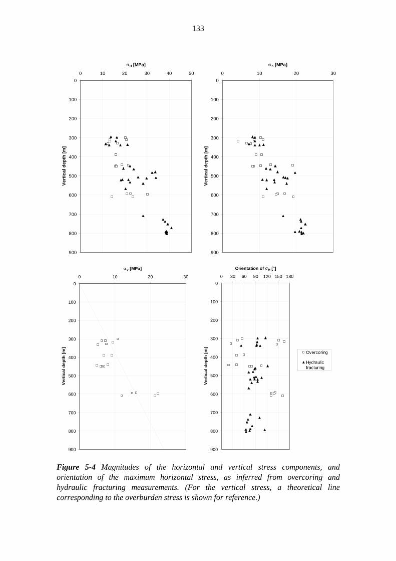
The results show increasing stress magnitudes with depth. The vertical and minimum horizontal stress components are fairly equal in magnitude, whereas the maximum horizontal stress is distinctly larger. The measured vertical stress is approximately equal to, or slightly lower than, the theoretical value corresponding to the overburden pressure. The orientation of the maximum principal stress (evaluated from overcoring) varies significantly between the boreholes, as well as between measurement levels and individual measurements in each borehole. There is thus a large uncertainty in the stress orientations, which is confirmed by the rather large confidence intervals obtained for all overcoring measurements (Figure 5-6 & Figure 5-7).

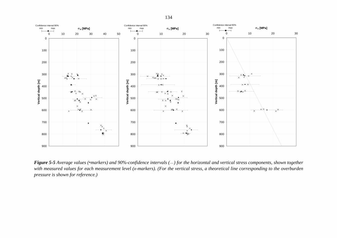
Since the principal stresses are not exactly in the horizontal-vertical planes, the horizontal and vertical stress components must be evaluated with some caution. The data indicate, however, that the maximum horizontal stress is oriented in a E-W to ENE-WSW direction (for both overcoring and hydraulic fracturing), but that the variation is quite large. The scatter in orientation data (for 90%-confidence intervals) is typically ±10-30° (occasionally larger). The scatter in magnitudes (for 90%-confidence intervals) is around ± 5 MPa for each measurement level.

The current data do not permit more elaborate interpretation with respect to geology and/or geological structures. Rather, linear regression lines were fitted to the data to arrive at preliminary equations for predicting the stress state. The regression lines obtained are shown in Figure 5-9. Data from both overcoring and hydraulic fracturing were used in deriving these equations — in fact, there was very little difference when applying regression to each data set individually as compared to lumping them together. The varying orientation of the horizontal components was not accounted for in this simplistic analysis. It is often inferred (from actual near-surface measurements and observations) that the stress state in Fennoscandia comprises a significant non-zero horizontal component near the ground surface. However, the regression analysis on the Olkiluoto data indicated very low stresses near the ground surface; hence, this intercept was set to zero for all stress components. A non-zero intercept could not be unambiguously defined based on the current data. For a target depth of 500 m, the resulting trend lines imply a maximum stress of around 24 MPa and a minimum stress of about 12 MPa. The obtained regression equations are as follows:

zH 047.0=σ , 300 < z < 800 m

zh 027.0=σ , 300 < z < 800 m

zv 024.0=σ , 300 < z < 800 m

where the stresses are expressed in MPa and

z = depth below the ground surface [m].

131

In summary, the current knowledge implies the following for the in situ stress state at Olkiluoto:

• Stress orientations are, on average, fairly consistent with the regional stress data, indicating a maximum horizontal stress oriented E-W to NW-SE. The site data support the notion of a thrust faulting stress regime at Olkiluoto, i.e., σH > σh > σv.

• The maximum horizontal stress has a gradient of, on average, 0.047 MPa/m, resulting in approximately 24 MPa at a target depth of 500 m. The vertical and minimum horizontal stresses are similar in magnitude, having a gradient which is about half that of the maximum stress, giving a magnitude of about 12 MPa at 500 m depth.

• The major principal stress (σ1 ) is sub-horizontally oriented, thus being slightly larger in magnitude than the maximum horizontal stress. The other two principal stress components vary significantly in magnitude and orientation for the different measurement locations. This indicates the need to relate the stress field with the geological structure and to conduct associated numerical analyses.

132

19.0119°/27°

11.8218°/17°

2.0337°/58°

449.29

16.5 92°/20°

13.2

195°/32°

0.6336°/51°

450.43

18.388°/23°

10.0191°/28°

3.2323°/53°

592.20

27.7

129°/34°

17.7

29°/14°

10.1280°/53°

595.48

25.8

135°/34°

15.1

228°/5°

10.0

325°/56°

597.39

31.3

136°/20°

21.7

359°/64°

13.9232°/17°

608.51

16.0

134°/34°

11.1232°/13°

10.1

340°/54°

610.20

23.8

341°/9°

21.2

142°/81°

19.2251°/3°

310.10

20.8

222°/7°

9.2129°/27°

6.5325°/62°

388.15

16.6269°/27°

15.1

15°/28°

4.1 143°/49°

390.05

16.1

220°/2°

9.3129°/15°

6.7316°/75°

OL-KR10 OL-KR24

300.26

22.6

217°/27°

16.0108°/32°

2.9338°/45°

309.06

14.8

136°/25°

11.4

41°/10°

4.3291°/63°

317.26

15.3

151°/34°

9.9

25°/42°

1.8264°/30°

328.10

18.0

199°/20°

9.9 91°/40°3.0308°/43°

331.48

15.0123°/30°

9.8

21°/20°

0.6263°/53°

441.75

20.2

52°/20°

14.6

150°/20°

5.0281°/61°

443.76

21.6

22°/3°

19.6112°/11°

4.3279°/79°

448.44

Figure 5-3 Measured principal stresses (magnitudes and trend/plunge) using overcoring at the Olkiluoto site. Each principal stress is represented by magnitude (length of vector; rotated onto the horizontal plane), trend (orientation of vector relative to north) and plunge (fan-shaped symbol; each fan-slice corresponds to 15° of dip from the horizontal).

133

0

100

200

300

400

500

600

700

800

900

0 10 20 30 40 50

σH [MPa]Ve

rtic

al d

epth

[m]

0

100

200

300

400

500

600

700

800

900

0 10 20 30

σh [MPa]

Vert

ical

dep

th [m

]

0

100

200

300

400

500

600

700

800

900

0 10 20 30

σV [MPa]

Vert

ical

dep

th [m

]

0

100

200

300

400

500

600

700

800

900

0 30 60 90 120 150 180

Orientation of σH [°]

Vert

ical

dep

th [m

]

Overcoring

Hydraulicfracturing

Figure 5-4 Magnitudes of the horizontal and vertical stress components, and orientation of the maximum horizontal stress, as inferred from overcoring and hydraulic fracturing measurements. (For the vertical stress, a theoretical line corresponding to the overburden stress is shown for reference.)

134

0

100

200

300

400

500

600

700

800

900

0 10 20 30 40 50

σH [MPa]

Vert

ical

dep

th [m

]

Confidence interval 90% min max

0

100

200

300

400

500

600

700

800

900

0 10 20 30

σh [MPa]

Vert

ical

dep

th [m

]


0

100

200

300

400

500

600

700

800

900

0 10 20 30

σV [MPa]

Vert

ical

dep

th [m

]


Figure 5-5 Average values ( markers) and 90%-confidence intervals (⎯ ) for the horizontal and vertical stress components, shown together with measured values for each measurement level (x-markers). (For the vertical stress, a theoretical line corresponding to the overburden pressure is shown for reference.)

135OL-KR10: Level 1, 90%-intervals

OL-KR10: Level 1, 95%-intervals




Figure 5-6 Confidence intervals (90%) for the orientation of the principal stresses determined from overcoring measurements at the Olkiluoto site in borehole KR10. (Note that 90%-intervals could not be calculated in some cases — for these, 95%-intervals are shown for comparison.)

136

OL-KR24: Level 1 (only one measurement)


Figure 5-7 Confidence intervals (90%) for the orientation of the principal stresses determined from overcoring measurements at the Olkiluoto site in borehole KR24. (Note that 90%-intervals could not be calculated in some cases — for these, 95%-intervals are shown for comparison.)

137

OL-KR1: Level 1

OL-KR1: Level 2

OL-KR2: Level 1

OL-KR2: Level 2

OL-KR2: Level 3

OL-KR4: Level 1

(only one measurement)

OL-KR4: Level 2

(only one measurement)

OL-KR10: Level 1

OL-KR10: Level 2 (only one measurement)

Figure 5-8 Confidence intervals (90%) for the orientation of the maximum horizontal stress determined from hydraulic fracturing measurements at the Olkiluoto site.

138

0

100

200

300

400

500

600

700

800

900

0 10 20 30 40 50

σH [MPa]Ve

rtic

al d

epth

[m]

0

100

200

300

400

500

600

700

800

900

0 10 20 30

σh [MPa]

Vert

ical

dep

th [m

]

0

100

200

300

400

500

600

700

800

900

0 10 20 30

σV [MPa]

Vert

ical

dep

th [m

]

Figure 5-9 Magnitudes of the horizontal and vertical stress components, shown with linear regression lines based on both overcoring and hydraulic fracturing measurements. (For the vertical stress, only overcoring data was used in the regression.)

139

5.4.2 Intact rock properties The mechanical properties of intact rock can, in general, be characterized by the complete stress-strain curve. This curve is obtained by compressing a cylindrical specimen, sawn from a diamond drilled core, in a servo-controlled testing machine. The stress-strain curve is used to select the appropriate conceptual model for intact rock and to define the associated parameter values (Figure 5-10).

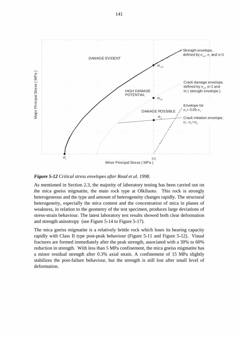
The stress-strain curve is divided into the pre-peak strength and post-peak strength regions. The pre-peak region for crystalline rock, as for the Olkiluoto rock types, is conceptualized to be mainly linearly elastic and isotropic or transversely isotropic; other assumptions are the continuity and homogeneity of the rock. The post-peak region, describing the microstructural breakdown of rock, is characterized by Classes I and II, depending on whether the strain increases monotonically (I) or not (II) with loss of bearing capacity (Figure 5-11). Since rock types do not behave ideally, two critical stress states are normally defined: the crack initiation stress when new stable microfracturing initiates; and crack damage strength when the extension of microcracking is unstable.

The critical stress states are stress state dependent, and normally they are assumed to be a function of the minor principal stress (Figure 5-12). The strength envelopes are commonly described by the Hoek-Brown criterion, the Mohr-Coulomb criterion, or by other criteria. In addition to the compression test, other commonly used tests are the indirect tensile test, the fracture toughness tests, the bending test, the point load index test and drilling parameter tests. The test should be conducted according to the ISRM Suggested Methods, because the specimen size and shape, saturation, loading control method and loading rate affect the results (see Section 2.3 for the Olkiluoto data). With the majority of these tests, acoustic emission measurements can also be used to obtain direct information on the microcracking (i.e. the total development of microcracking: its initiation, stable increase, unstable increase, larger occurrences).

140

Axial Stress( MPa )

20

40

60

80

100

120

-0.15 -0.10 -0.05 0.05 0.10 0.20 0.250.15Radial Strain ( % ) Axial Strain ( % )

Elastic region II

Unstable crack IVgrowth

Stable crack IIIgrowth

Crack closure I

Onset of post-peak region V - temporary hardening

Crack Damage Stress- true peak strength

σcd

Crack Initiation Stress- beginning of damage

σci

-0.15

-0.10

-0.05

0

0.05

0.10

0.0 0.05 0.10 0.15 0.20

VolumetricStrain ( % )

0.25

Axial Strain ( % )

I

IIIII IV

Crack Closure Calculated CrackVolumetric Strain

Measured totalvolumetric strain

New Crack Volume

Axial StressAxial Strain

RadialStrain

Natural Microcracks

Peak Strength σp

Tensile Strength σt

Figure 5-10 Characteristic stress-strain behaviour of brittle rock (according to Martin 1994).

Figure 5-11 Definition of Class I and Class II post peak behaviour (Wawersik 1968).

141

0.0Minor Principal Stress ( MPa )

Maj

or P

rinci

pal S

tress

( M

Pa

)

σcd

σci

Strength envelope,defined by , and s=1σ σucs t

σt

σucs

Crack initiation envelope,- σ σ1 ciσ3 =

Crack damage envelope,defined by , s=1 σcd andm ( strength envelope )

Envelope for= 0.05 σ3 σ1

HIGH DAMAGEPOTENTIAL

DAMAGE POSSIBLE

DAMAGE EVIDENT

Figure 5-12 Critical stress envelopes after Read et al. 1998.

As mentioned in Section 2.3, the majority of laboratory testing has been carried out on the mica gneiss migmatite, the main rock type at Olkiluoto. This rock is strongly heterogeneous and the type and amount of heterogeneity changes rapidly. The structural heterogeneity, especially the mica content and the concentration of mica in planes of weakness, in relation to the geometry of the test specimen, produces large deviations of stress-strain behaviour. The latest laboratory test results showed both clear deformation and strength anisotropy (see Figure 5-14 to Figure 5-17).

The mica gneiss migmatite is a relatively brittle rock which loses its bearing capacity rapidly with Class II type post-peak behaviour (Figure 5-11 and Figure 5-12). Visual fractures are formed immediately after the peak strength, associated with a 30% to 60% reduction in strength. With less than 5 MPa confinement, the mica gneiss migmatite has a minor residual strength after 0.3% axial strain. A confinement of 15 MPa slightly stabilizes the post-failure behaviour, but the strength is still lost after small level of deformation.

142

Axial Stress ( MPa )

Radial Strain Axial Strain

-25

0

25

50

75

100

125

150

175

200

225

250

-1.2% -0.8% -0.4% 0.0% 0.4% 0.8%

Olkiluoto KR10 Mica Gneiss Uniaxial compression tests, n=60

Triaxial compression tests =15 MPa, n=8

σc

OLKR10-1A-574.15

OLKR10-3A-576.55

Figure 5-13 Envelopes of the variation in uniaxial and triaxial stress-strain behaviour of Olkiluoto mica –gneiss migmatite and two typical stress-strain curves (Hakala & Heikkilä,1997b).

Assuming transverse isotropy, the deformation anisotropy for Olkiluoto mica gneiss migmatite is about 1.4 ( E/E′) (Table 5-1 and Figure 5-14), where E is the Young’s modulus parallel to the foliation, and E′ perpendicular to the foliation. The apparent deformation parameters for different loading conditions are summarized in Table 5-2. The development of damage, which is defined as permanent volumetric inelastic strain accumulated in the sample with each loading cycle, induces large deviation in the apparent Young’s modulus and Poisson’s ratio. Damage, after the first detection of crack damage stress in damage controlled tests, changes the apparent elastic parameter. During the first 0.1% strain, the apparent Young’s modulus decreases by approximately 10 GPa / 0.1% strain and, after that, approximately 3 GPa / 0.1% strain. The apparent Poisson’s ratio increases approximately 0.1 / 0.1% strain and exceeds the theoretical maximum of 0.5 for an isotropic elastic rock at the point of formation of the visual fracture.

143

Table 5-1 Elastic deformation parameters for Olkiluoto mica gneiss migmatite assuming transverse anisotropy (Hakala & Kuula 2004).

Young’s modulus parallel to foliation E 79 GPa Young’s modulus transverse foliation E´ 56 GPa Poisson’s ratio parallel to foliation n 0.17 mm/mm Poisson’s ratio transverse foliation n´ 0.21 mm/mm Shear modulus G 24.1 GPa

Table 5-2 Apparent elastic deformation parameters for Olkiluoto mica gneiss migmatite under different loading conditions.

Parameter Loading condition Average 95% confidence for standard deviation

Number of

samples

Young’s modulus, E direct tension 43 GPa 19 GPa 20 uniaxial, 0.0075 MPa/s 57 GPa 14 GPa 15 uniaxial, 0.75 MPa/s 63 GPa 12 GPa 63 triaxial, sc = 0.5-15 MPa 63 GPa 10 GPa 40 Poisson’s ratio ν direct tension 0.06 mm/mm 0.03 mm/mm 20 uniaxial, 0.0075 MPa/s 0.28 mm/mm 0.05 mm/mm 15 uniaxial, 0.75 MPa/s 0.25 mm/mm 0.06 mm/mm 63 triaxial, sc = 0.5-15 MPa 0.20 mm/mm 0.05 mm/mm 40

0

10

20

30

40

50

60

70

80

90

100

0 20 40 60 80 100( GPa )

(GPa

)

E=40GPa

E=60GPa

E=80GPa

LS-Fit for Aniso ModelMeasured

15°

30°

45°

60°

75°

0

10

20

30

40

50

60

70

80

90

100

0 20 40 60 80 100( GPa )

(GPa

)

E=40GPa

E=60GPa

E=80GPa


15°

30°

45°

60°

75°

0

10

20

30

40

50

60

70

80

90

100

0 20 40 60 80 100( GPa )

(GPa

)

E=40GPa

E=60GPa

E=80GPa


15°

30°

45°

60°

75°

Figure 5-14 Apparent Young’s modulus for Olkiluoto mica gneiss in different loading directions as a function of the schistosity/foliation (assumed as a plane for transverse anisotropy) (Hakala & Kuula, expected 2005).

144

The tensile strength of Olkiluoto mica gneiss migmatite is most sensitive to anisotropy, whereas the crack initiation stress is, perhaps counter-intuitively, the least sensitive (Figures 5-15 to 5-18). Noteworthy is the large overlap of the standard deviation values. Other apparent strength values for mica gneiss migmatite are listed in Table 5-3.

0.0

5.0

10.0

15.0

20.0

25.0

0 10 20 30 40 50 60 70 80 90

Anisotropy angle ( degrees )

Tens

ile s

tren

gth

( M

Pa )

Effect of Anisotropy on Indirect Tensile strength- Average, standard deviation and number of tests values for three anisotropy angle regions

16.5 MPa2.1 MPan=8

14.1 MPa2.3 MPan=5

12.5 MPa2.4 MPan=5

Figure 5-15 Effect of anisotropy on the indirect tensile strength of dry Olkiluoto mica gneiss migmatite.

0

25

50

75

100

125

150

175

0 10 20 30 40 50 60 70 80 90


Cra

ck in

itiat

ion

stre

ss (

MPa

)

Effect of Anisotropy on Crack Initiation Stress- Average, standard deviation and number of tests values for three anisotropy angle regions- Crack initiation stress is 41% - 49% of peak strength

55 MPa4.4 MPan=8

56 MPa15.8 MPan=5

55 MPa8.9 MPan=5

Figure 5-16 Effect of anisotropy on crack initiation strength of dry Olkiluoto mica gneiss migmatite.

145

0

25

50

75

100

125

150

175

0 10 20 30 40 50 60 70 80 90


Cra

ck d

amag

e st

ress

, ( M

Pa )

Effect of Anisotropy on Crack Damage Stress- Average, standard deviation and number of tests values for three anisotropy angle regions- Crack damage stress is 91% - 97% of Peak strength

125 MPa18.6 MPan=8

110 MPa15.6 MPan=5

129 MPa26.5 MPan=5

Figure 5-17 Effect of anisotropy on the crack damage stress value of dry Olkiluoto mica gneiss migmatite.

0

25

50

75

100

125

150

175

0 10 20 30 40 50 60 70 80 90


Peak

str

engt

h (

MPa

)

Effect of Anisotropy on Peak Strength- Average, standard deviation and number of tests values for three anisotropy angle regions

137 MPa16.1 MPan=8

113 MPa18.3 MPan=5

132 MPa29.8 MPan=5

Figure 5-18 Effect of anisotropy on the peak strength of dry Olkiluoto mica gneiss migmatite.

146

Table 5-3 Apparent elastic deformation parameters for Olkiluoto mica gneiss migmatite under different loading conditions (if not mentioned, the tested specimens are saturated).

Parameter Loading condition Average value 95% confidence limit for standard

deviation

Number of

samples

Tensile strength, σt direct tension 7.9 MPa 2.2 MPa 19 indirect, saturated 10.0 MPa 3.2 MPa 30 indirect, dry 14.5 MPa 3.6 MPa 23 Crack initiation, σci direct tension 2.5 MPa 1.4 MPa 4 uniaxial, 0.0075 MPa/s 45 MPa 15 MPa 15 uniaxial, 0.75 MPa/s 54 MPa 15 MPa 54 Crack damage, σcd direct tension 5.8 MPa 3.2 MPa 4 uniaxial, 0.0075 MPa/s 76 MPa 27 MPa 13 uniaxial, 0.75 MPa/s 106 MPa 29 MPa 53 Peak strength, σP uniaxial, 0.0075 MPa/s 96 MPa 34 MPa 13 uniaxial, 0.75 MPa/s 115 MPa 28 MPa 72

The critical stress envelopes for Olkiluoto mica gneiss migmatite are defined by using the average stress state values in both tension and in uniaxial loading; this method ensures that the tensile strength is calculated correctly (Table 5-4). The original method of defining the Hoek and Brown envelope values is to fit an envelope based on uniaxial and triaxial test results and apply a tension cut-off to establish the tensile strength.

Table 5-4 Critical stress envelopes for Olkiluoto mica gneiss migmatite, according to the method of Read et al. 1998 (for saturated specimens, the Mohr-Coulomb fit is tangent at σ3=0).

Critical stress σ1 (σ3 = 0) HB-mi σT c φ MPa MPa MPa ° Peak 115 9.563 12.0 21.2 49 Crack damage 106 9.563 5.8* 19.4 48 Crack initiation 53 1.0 2.5* 20.7 16 * The Hoek & Brown envelope must be truncated, values based on acoustic emission measurements by Hakala & Heikkilä (1997b). The post-failure behaviour of all critical stress states was of the Class II type. The effect of a confinement pressure of less than 3 MPa is minor and the effect of damage on crack initiation and crack damage was rapid during the first 0.2% to 0.3% damage (Figure 5-19 and Figure 5-20). In all the uniaxial cases, the crack damage stress equals the crack initiation stress up to 0.2% damage and in the majority of the 3 MPa confined tests, the corresponding damage level was 0.3%. At the point, when the crack damage

147

stress is coincident with the crack initiation stress, the 95% confidence limits for axial stress are 20 MPa and 55 MPa. After this point, the post-failure behaviour is defined by the geometry of the visual fracture compared to the specimen geometry and the amount of confinement.

0

25

50

75

100

125

150

0.0% 0.2% 0.4% 0.6% 0.8% 1.0%

Crack InitiationCrack DamagePeak

Critical Stress ( MPa )

Olkiluoto Mica GneissUniaxial Damage Controlled Test,n = 6

Damage ( mm /mm )3 3

Figure 5-19 Development of critical stress states in uniaxial damage controlled tests after the first detection of crack damage stress (Hakala & Heikkilä, 1997b).

The critical strength and elastic property values for other rock types do not differ significantly from mica gneiss migmatite, except for the lower crack initiation of granite/pegmatite (Table 5-5). A summary of the laboratory test results is shown in Table 5-5. It should be noted that values presented in the table are mostly measured on water-saturated rock samples, since the in situ conditions are wet. Values of tensile strength for wet samples are about 10 - 30 % lower than those for dry samples.

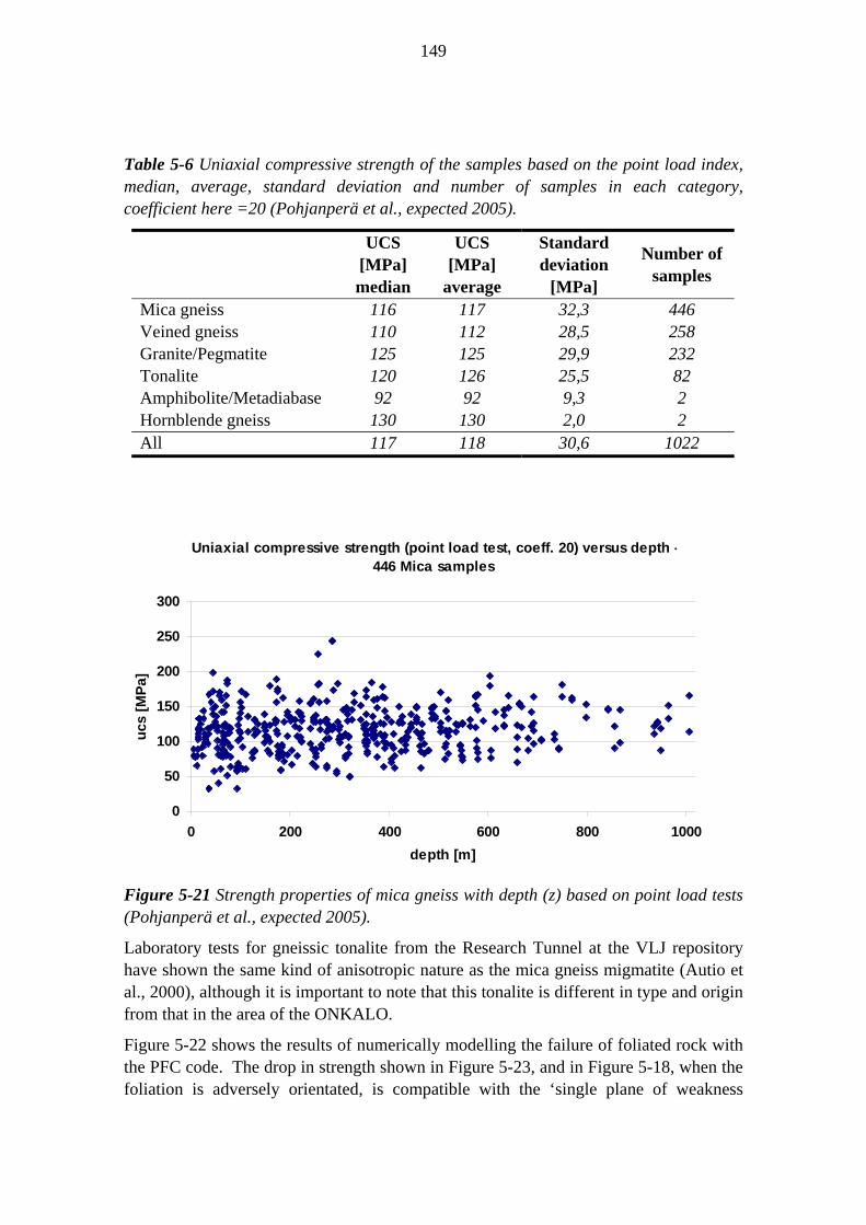
A summary of uniaxial compressive strengths from the field tests for 29 deep boreholes (KR1- KR28 and PH1) is presented in Table 5-6. The strength values given in the table are calculated using the point load index and a conversion factor, which is dependent on the rock type. Thus, the field values cannot be directly compared to the laboratory values, but give relative strength values for different rock types. The results are classified according to the rock type under six rock type categories. The classification for a few rock samples was uncertain and these were omitted. The depth dependence was also studied and it was found that the strength values show no correlation with depth (Figure 5-21).

148

0

25

50

75

100

125

150

0.0% 0.2% 0.4% 0.6% 0.8% 1.0%

Critical Stress ( MPa )

σc

Olkiluoto Mica GneissTriaxial Damage Controlled Test,

= 3 MPa, n = 10

Damage ( mm /mm )3 3

Crack InitiationCrack DamagePeak

Figure 5-20 Development of critical stress states in triaxial damage controlled tests after the first detection of crack damage stress, all observations and envelopes (Hakala & Heikkilä, 1997b).

Table 5-5 Strength and deformation properties of rock types at Olkiluoto based on laboratory tests. The values presented are arithmetical means with standard deviations in parentheses; N = number of samples. The sample diameter varied from 42 – 62 mm. The peak strength values are scaled to 62 mm specimen size (Äikäs et al. 2000).

Rock type/ Property

Crack initiation

strength σci (MPa)

Long term strength σcd

(MPa)

Peak strength

σucs (MPa)

Tensile strength

σt (MPa)

Young’s modulus E (GPa)

Poisson’s ratio

ν

Mica gneiss migmatite

52.6 (11.8) N = 54

106.4 (23.7) N = 53

114.9 (23.1) N = 72

12.0 (3.3)

N = 53

62.6 (9.9)

N = 63

0.25 (0.05) N = 63

Granite/ pegmatite

30.1 (8.3) N = 2

107.5 (23.7) N = 2

133.8 (18.5) N = 5

69.6 (5.7) N = 5

0.30 (0.04) N = 5

Grey (tonalite) gneiss

109.5 (7.8) N = 4

64.5 (1.7) N = 4

0.28 (0.02) N = 4

σucs-strength = uniaxial compressive strength (UCS), peak strength

σcd-strength = stress level at which unstable microfracturing begins in sample

σci-strength = stress level at which the microfracturing or damage initiates in sample Tensile strength σt = determined by Brazilian test (the direct tension test (N = 19) gave a value

7.9 MPa for mica gneiss)

149

Table 5-6 Uniaxial compressive strength of the samples based on the point load index, median, average, standard deviation and number of samples in each category, coefficient here =20 (Pohjanperä et al., expected 2005).

UCS [MPa] median

UCS [MPa]

average

Standard deviation

[MPa]

Number of samples

Mica gneiss 116 117 32,3 446 Veined gneiss 110 112 28,5 258 Granite/Pegmatite 125 125 29,9 232 Tonalite 120 126 25,5 82 Amphibolite/Metadiabase 92 92 9,3 2 Hornblende gneiss 130 130 2,0 2 All 117 118 30,6 1022

Uniaxial compressive strength (point load test, coeff. 20) versus depth -446 Mica samples

0

50

100

150

200

250

300

0 200 400 600 800 1000depth [m]

ucs

[MPa

]

Figure 5-21 Strength properties of mica gneiss with depth (z) based on point load tests (Pohjanperä et al., expected 2005).

Laboratory tests for gneissic tonalite from the Research Tunnel at the VLJ repository have shown the same kind of anisotropic nature as the mica gneiss migmatite (Autio et al., 2000), although it is important to note that this tonalite is different in type and origin from that in the area of the ONKALO.

Figure 5-22 shows the results of numerically modelling the failure of foliated rock with the PFC code. The drop in strength shown in Figure 5-23, and in Figure 5-18, when the foliation is adversely orientated, is compatible with the ‘single plane of weakness

150

theory’ which applies for a single fracture and can also be applied to the weakness introduced by the foliation.

Initiation Fracture growth Failure Collapse

Figure 5-22 Simulation of foliated rock failure using the code PFC3D (from Wanne 2002). Note the ‘U’ shaped curve which follows the ‘single plane of weakness’ theory.

5.4.3 Physical properties In the laboratory, the dry density and porosity can be defined and measured according to the ISRM Suggested Methods. These values were measured for Olkiluoto mica gneiss migmatite and pegmatite using water immersion, storing at 100% humidity, and drying at 102°C, which is the method suggested by the ISRM (Hakala and Heikkilä, 1997a). The defined porosity describes the amount of the open pore volume for groundwater penetration. The compressive P-wave velocity is defined, according to the ISRM suggested method, using a dried specimen. The transducer and receiver are pressed onto the specimen ends with a constant axial contact pressure of 65 kPa and the wave transmission on contact is improved with water (water is used as couplant only on the contact surfaces).

151

The average dry density of Olkiluoto mica gneiss migmatite, based on 122 specimens, is 2734 kg/m3 with a deviation of 33 kg/m3. The corresponding values for pegmatite based on 10 specimens is 2608 kg/m3 and 25 kg/m3.

The average porosity of Olkiluoto mica gneiss migmatite based on 120 specimens is 0.23% with a deviation of 0.088%. The corresponding values for pegmatite based on 10 specimens is 0.37% and 0.069%.

5.4.4 Thermal properties The thermal properties of the rock are required as input data for determining the dimensions of the disposal rooms and for evaluating the thermal stresses induced by heat produced by the radioactive waste. The thermal properties of intact rock are determined mainly by their mineralogical composition. The average thermal conductivity of feldspars and micas is typically 2.0 - 2.5 W/(mK); however, the conductivity of quartz is significantly higher at 7.7 W/(mK). Most minerals are thermally anisotropic, and micas (biotite, muscovite) are particularly anisotropic, showing large variation in thermal conductivity depending on the direction of the measurement. Thermal properties are also temperature-dependent and thermal conductivity and diffusivity decrease and heat capacity increases with increasing temperature (Kukkonen & Lindberg 1995; Kukkonen 2000).

The measured thermal properties of the rock types at Olkiluoto are presented in Table 5-7. The mica gneiss migmatite is thermally anisotropic and heterogeneous due to variations in its texture, mineral composition and the orientations of the migmatitic banding and the foliation. The typical range of thermal conductivity for the mica gneiss migmatite is 2.3 – 2.8 W/mK, where the minimum value 2.3 W/mK is interpreted to represent the value perpendicular to the foliation (Kukkonen 2000). The mean anisotropy factor based on measurements of a few samples is about 1.3. The thermal conductivity of the mica gneiss migmatite calculated from the average mineralogical composition gives a value of 2.52 W/mK (harmonic mean).

152

Table 5-7 The thermal properties of the main rock types at Olkiluoto (Kukkonen 2000). The properties are average values (arithmetical mean) with standard deviations in parentheses, N = number of samples.

Rock type/Parameter Thermal conductivity

(W/(mK))

Thermal heat capacity (J/(kgK))

Thermal diffusivity * (10-6 m2/s)

Coefficient of thermal

expansion (10-6/°C)

20 - 22 °C 99 °C 10 – 60 °C Mica gneiss migmatite 2.7 (0.4)

N = 42 832 (19) N = 42

1.18 (0.2) N = 42

9.5 (2.4) (7-10**) N = 3

Granite/pegmatite 4.2 (0.5) N = 2

778 (6.0) N = 2

1.18 (0.06) N = 2

Grey (tonalite) gneiss 2.7 (0.1) N = 2

797 (3.5) N = 2

1.23 (0.06) N = 2

* calculated from conductivity, heat capacity and rock density ** estimated range from Huotari & Kukkonen 2004

5.4.5 Drilling properties The drilling parameters DRI (Drilling Rate Index) and CAI (Cerchar Abration Index) have also been determined for mica gneiss migmatite and grey (tonalite) gneiss at Olkiluoto (Äikäs et al. 2000) and estimated values of these parameters for the other rock types have been made on the basis of a literature review. The Vickers hardness of the rock types was calculated on the basis of the average mineral composition determined from thin section analysis and the results are shown in Table 5-8. With regard to the drilling properties, all the rock types at Olkiluoto are placed in the normal class of constructability, regardless of the drilling method (Äikäs et al. 2000).

Table 5-8 Drilling parameters, strength and Vickers hardness for different rock types. The values presented are arithmetical means with standard deviations in parentheses (Äikäs et al. 2000).

Rock type DRI index (defined)

DRI index (literature)

CAI index Peak strength (range MPa)

Vickers (average)

Vickers (range)

Mica gneiss migmatite

45 ( 4.3 ) 50-70 4.3 ( 0.1 ) 80 – 140 713 382 - 948

Granite/ pegmatite

- 45 – 65 (granite)

- 115 – 150 807 720-895

Grey (tonalite) gneiss

55 ( 3.0 ) 45 – 65 * 3.7 ( 0.4 ) 80 – 110 672 535 - 822

Amphibolite/ metadiabase

- 40 - 60 (amphibolite) 30 – 45 (metadiabase)

100 559 410-708

* no values for grey (tonalite) gneiss were available, so the value for granite is applied here

153

5.4.6 Mechanical properties of fractures A typical feature of the bedrock at Olkiluoto is the presence of pre-existing fractures. The mechanical strength and deformation properties of the fractures are dependent on several features, such as the undulations and roughness of the fracture surfaces, their trace length, the occurrence of slickensides, the quality and thickness of the fracture fillings, as well as the strength of the surrounding rock and the in situ stress. The properties of fractures are particularly significant in determining the mechanical behaviour of fracture zones, where the fracture frequency is higher and the frictional properties of fractures less than in much of the rock mass.

Fracture sets have been established via the geological studies, but over large areas, and further work is required to determine the geometry of the fractures in specific volumes of rock at the tunnel scale. The mechanical properties of fractures at Olkiluoto have not been measured directly in the laboratory, but can be and have been estimated on the basis of the geological description of fractures, as shown in Rautakorpi et al. (2003). It has been established that, for example, low-dipping fractures may have lower strengths than sub-vertical fractures. Some joint tests performed for the VLJ repository at Olkiluoto indicate a friction angle of 26 - 35°and a cohesion of 660 - 900 kPa in fractures in tonalite and in mica gneiss migmatite (Kuula & Johansson 1991).

5.4.7 Mechanical properties of brittle deformation fracture zones (R and RH structures)

Several fracture zones have been observed at Olkiluoto. In rock mechanics analyses the properties of fracture zones (weakness zones) can be treated in different ways, depending on the scale and the structure of the zone. Figure 2-10 summarizes the commonly used modelling concepts and the associated mechanical material properties.

The most common procedure to determine the properties of fracture zones is by rock engineering classification, such as the use of the Q-method, which has been used at Olkiluoto (Äikäs et al. 2000). In addition to this empirical rock mass classification, there are also published data available and some simple analytical methods in which the properties of intact rock and fractures are combined to yield the fracture zone properties. A more detailed description of the fracture zone properties and how they are determined can be found in Posiva (2003a).

A study was carried out by Johansson et al. (2002) to characterize the fracture zones over the depth interval of 400 – 500 m. The Q′-values (the Q-value excluding the depth-dependent parameters of stress and the effects of groundwater) were calculated for the fracture zones intersected in several deep boreholes. The average values of Q′ and RQD are presented in Table 5-9 for all fracture zones and, in addition, these parameters are presented separately for gently-dipping fracture zones (dip < 45º) and steeply-dipping fracture zones (dip > 45º). The steeply-dipping fracture zones have slightly lower Q′-values, whereas the average RQD is nearly the same. The number of data was rather sparse, particularly for the steeply-dipping fracture zones and it should be noted that

154

these properties have been determined exclusively from borehole data, and therefore refer only to the locations where the deep boreholes intersect these zones.

The fracture frequency and extent of a fracture zone is likely to be different depending on the intersection angle of the borehole with the zone. In the analysis referred to above the boreholes are mainly sub-perpendicular to the zones, so the estimates are likely to be reasonably representative. The fracture frequency and the Ri-class (fracturing class) of these ten fracture zones were examined in Johansson et al. (2002) based on the Finnish engineering geological rock classification system. The majority (six) of the fracture zones studied contained RiIII sections (i.e. where fracture frequency > 10 fractures/m and where there is minor filling in fractures). Only the largest two fracture zones also had RiIV sections (fracture frequency 3 - 10 or > 10 fractures/m and fractures filled with clay minerals). The average fracture frequency of the fracture zones was seven fractures/m, both for gently-dipping and steeply-dipping zones (however, in three fracture zones the number of fractures in some broken core sections could not be measured, and only the measured fractures were included in the analysis). Taking only the fracture zones and fracture zone segments with a width of < 5 m into account, the average fracture frequency is 10 fractures/m.

Table 5-9 Q′ (geometric mean), Q, Erm deformation modulus and RQD (arithmetic mean) of fracture zones intersected by eight deep boreholes at Olkiluoto at the approximate depth interval –400–500 m (modified from Johansson et al. 2002).

Fracture zones/Rock mass quality

Q′ Q* Deformation modulus Erm

(GPa)**

RQD Number of fracture

zones

Borehole length (m)

All fracture zones 5.5 11.0 24.5 78.7 10 89 Gently-dipping fracture zones (dip < 45º)

5.8 11.6 24.9 78.4 7 72

Steeply-dipping fracture zones (dip > 45º)

4.5 9.0 22.9 79.9 3 17

* assuming Jw=1, SRF=0.5 ** calculated from Eq. Erm=10xQc

1/3, Qc=Qx(σc/100), σc= 110 MPa

5.4.8 Mechanical properties of the rock mass (volume) The properties of the rock mass (intact rock matrix + fractures but excluding fracture zones), as for the fracture zones described above, can also be evaluated based on rock engineering classifications. The results of such a classification of the rock mass with depth are presented in Table 5-10. The Q-values have been determined for 50 m intervals; however, in the future, it will be possible to calculate the Q-values over geological domains. The results here are those for all the rock types at Olkiluoto - mica gneiss migmatite, grey (tonalite) gneiss and granite. Q-values are found to be somewhat lower in the upper part of the bedrock (0 - 150 m) than at greater depths (> 150 m), where they are largely independent of depth. This conclusion is also supported by the seismic velocity measurements. The Q-values for the rock mass are about three to four times greater than those for the fracture zones (Table 5-10). It should be noted that the

155

rock mass strength calculated from the Q-value and shown in Table 5-10 is very close to the crack initiation strength of a rock sample presented in Table 5-5.

Table 5-10 Variation of Q values (geometric mean) for the Olkiluoto rock mass with depth and including the factors of high stress, tight structure, Erm deformation modulus and σrm rock mass strength (boreholes KR1 – KR12) (Posiva 2003a).

Vertical depth (m)

Q* (mean)

Deformation modulus

E (GPa)**

Rock mass strength

(MPa)***

N (borehole

meter) 0...150 29.6 31.9 43.8 1272 150...200 42.0 35.9 49.2 634 200...250 35.9 34.1 46.7 555 250...300 31.4 32.6 44.6 571 300...350 41.5 35.7 49.0 544 350...400 36.5 34.2 46.9 533 400...450 37.1 34.4 47.2 550 450...500 43.6 36.3 49.8 488 500...550 40.0 35.3 48.3 376 550...600 42.3 36.0 49.3 316 600...650 41.8 35.8 49.1 302 650...700 45.8 36.9 50.6 298 700...750 47.4 37.4 51.2 275 750...800 37.0 34.4 47.1 242 800...850 40.5 35.5 48.6 208 850...900 41.9 35.9 49.1 163 900...1000 36.9 34.4 47.1 153

* Q-value assuming Jw=1, SRF=0.5 (assumed fixed for comparison purposes) **calculated from Eq. Erm=10xQc

1/3, Qc=Qx(σc/100), σc= 110 MPa *** calculated from Eq. σrm=5xγxQc

1/3, γ=density

The P-wave velocities of the bedrock at the surface determined from refraction seismic, which describe the uppermost 15 - 20 m of the bedrock, range from 3400 m/s to 5500 m/s. Velocities below 4000 m/s represent potential highly-fractured sections and account for about 8 - 10% of the bedrock surface area (Lehtimäki 2003a). Velocities greater than 4500 m/s are dominant and there is no marked seismic anisotropy, as the difference in velocity measured in different directions is only 1-2%.

Typical seismic velocities at depth are 5600 - 5750 m/s, based on the velocity model of large-scale VSP reflection data that have been fitted to measured travel times and then used in VSP reflector interpretations (e.g. Cosma et al. 2003). The narrow fracture zones and the high-velocity amphibolite or metadiabase dykes do not alter this velocity pattern, except that they can typically cause some 1-3 millisecond delays to the seismic wave travel time. In the area of borehole KR6 a macroscopic 15 - 20% velocity anisotropy has been recognised due to a thick low velocity layer. There is no evidence of the presence of other areas of significant anisotropy (Cosma et al. 2003) or of transverse isotropy.

156

Wireline acoustic logging shows that the P-wave velocity increases with depth from 20 - 150 m from 4500 m/s to 5300 m/s. This is the same depth interval in which the majority of the near-surface fracturing is encountered.

At greater depth the P-wave velocities are largely independent of depth. Typical velocities in bedrock of 0-3 fractures per metre are 5500 m/s; bedrock with fracture frequencies of 3-10 has velocities of 4500 - 5000 m/s, and more highly fractured bedrock, > 10 fractures per metre, which is typically present as narrow sections, has velocities of 3500 - 4500 m/s.

The S-wave velocities vary from 3200 - 3300 m/s in sparsely fractured rock to 2500 - 3000 m/s in fracture zones. Typical P- and S-wave velocities in sparsely fractured mica gneiss migmatite, grey (tonalite) gneiss and granite pegmatite are 5400 m/s and 3300 m/s, respectively, and the rock densities range from 2.59 to 2.75 kg/dm3. The P and S-velocities are highest (6400 m/s and 3500 m/s, respectively) in amphibolite-bearing or metadiabase layers, where the density is also highest (close to or greater than 3.0 kg/dm3) (Julkunen et al. 2002, Lahti et al. 2001, 2003, Front et al. 2002; Lahti & Heikkinen 2004).

The range of dynamic elastic moduli and other derived rock mechanics parameters have been listed in Table 5-11 below (Front et al. 2002, Lahti & Heikkinen 2004) and in Figure 5-23.

Table 5-11 Elastic properties in Olkiluoto bedrock as derived from acoustic and density parameters.

Parameters Region P wave velocity

(m/s)

S wave velocity

(m/s)

Density (g/cm3)

Deformation modulus

(Edyn, GPa)

Shear modulus

(Mdyn, GPa)

Poisson’s ratio

Surface part of bedrock 0-100 m

4500-5300

2400-2800 2.6-3.2 38 - 55 10-25 0.2 - 0.35

Fracture zones

3500-4800

2000-2500 2.4-3.2 38 - 55 GPa (lowest 25)

10-25 0.1 - 0.15

Intact bedrock

5500-6500

2900-3300 2.6-3.2 60 to 75 25-30 0.15 - 0.30

Mica gneiss (intact)

5500-5800

2900-3200 2.65-2.8 61 - 64 25-30 0.25 - 0.30

Granite, Pegmatite (intact)

5600-5900

2900-3200 2.59-2.75

65 - 70 22-28 0.25-0.28

Grey gneiss (intact)

5900-6200

3000-3300 2.8-3.0 73 - 75 25-35 0.30-0.32

Amphibolite, Metadiabase (intact)

6000-7000

3200-3600 2.9-3.3 80 - 100 30 - 45

157

Figure 5-23 Acoustic measurement data and derived parameters from borehole OL-KR29. The gamma-gamma density and P and S-wave velocities were used to compute the dynamic mechanical parameters (Lahti & Heikkinen, 2005). Depth range 40-800 m.

Mechanical parameters vary in the rock mass, being lowest near the surface and in fracture zones, and highest at greater depth. In the zones of more intense fracturing the value of the deformation modulus can be as low as 25 GPa.

No exhaustive analysis of these properties with respect to rock type has been carried out, but the values seem to be most uniform in grey (tonalite) gneiss sections, and most

158

variable in mica gneiss migmatite sections (due to the presence of fractures and to variations in neosome-palaeosome distributions) and possibly slightly higher in granite pegmatite than in mica gneiss. The highest values are encountered in amphibolite-bearing rock types or in metadiabase.

The dynamic Poisson’s ratio typically varies from 0.19 - 0.25 and appears to be highest in grey (tonalite) gneiss, granite pegmatite and the amphibolite or metadiabase, and lowest in mica gneiss migmatites. The lowest values of 0.1-0.15 have been encountered in narrow sections containing clay- and grain-filled, or open fracturing.

The greatest variation in the parameters has been in the most fractured upper part (40 - 100 m) of the bedrock, as well as in sections where sulphides increase the density of the rock mass.

The dynamic modulus for mica gneiss is consistent with the laboratory values and the Young’s modulus determined from depth-adjusted Q-values (Barton 2002, see above). The differences in these values may arise from the different scales involved and may be partly due to differences in the definitions of the laboratory and dynamic parameters. It also may indicate the influence of increasing stress due to depth (due to the closure of microcracks). The dynamic parameters are also influenced by the presence of fracturing, whereas the laboratory specimens are, by definition, from non-fractured rock.

5.4.9 Bedrock stability measurements No observations of seismic activity have been recorded up to the end of November 2004. The result was expected, because i) the monitored area is rather small and it is located in an area of low tectonic activity and ii) the access tunnel has not yet reached a substantial depth. Observations of tectonic activity are more likely when the network is expanded and when the time period is longer. Excavation induced perturbations are expected at larger depths, where the stress is higher and, especially, when the excavation approaches and runs through a brittle deformation zone.

GPS measurements have been carried out since 1995 and the results to date show that the measured changes are small. The analysis of 16 series of GPS measurements shows that there are only two baselines in which the rates of change exceed 0.3 mm/y (Ollikainen et al. 2004) and statistical analysis shows that there are no baselines with rates of change which are statistically significant at the 95%-confidence level. The agreement between GPS and Electronic Distance Measurement (EDM) is good.

5.5 Evaluation of uncertainties This section evaluates the uncertainties in the various components of the Rock Mechanics modelling.

5.5.1 Evaluation of uncertainties relating to in situ stress Stress is a tensor quantity with six independent components and is defined at a point in the rock mass. It is not possible to measure stresses directly: only normal stress components and normal strains can be measured; shear stresses and shear strains cannot

159

be measured directly. So, all stress measurement methods are indirect in nature (to various degrees), from which the in situ stress state can be inferred. The overcoring method relies, for example, on the measurement of strains, which can be related to stresses under certain assumptions of ideal behaviour; whereas, in hydraulic fracturing, water pressures are measured, which then can be related to the acting normal in situ stress component across a fracture.

It is inappropriate to discuss the accuracy of stress measurements (i.e. how close the measured values are to the true values), since the actual stress state in the field is not known beforehand. The precision, on the other hand (defined as a measure of the variation in measurement data), can be used to assess the scatter in individual values for a particular group of measurements. Amadei & Stephansson (1997) stated that the expected imprecision is at least 10-20%, even in rock masses that fulfil all the basic assumptions of the method. Leijon (1988) concluded that non-systematic measurement errors had a standard deviation of 2 MPa or less; whereas, repeated measurements showed a standard deviation of up to 4 MPa (depending on the rock type). Sjöberg & Klasson, 2003, found that the typical imprecision for overcoring measurements using the Borre probe was at least 1-2 MPa in absolute numbers, with an additional relative imprecision of ± 10% (or more).

The scatter in the Olkiluoto data (cf. Figure 5-5 to Figure 5-8) is thus fairly typical for the methods employed. It can be seen that the scatter in overcoring data is larger than for hydraulic fracturing, which can partly be attributed to the fact that the representative volume of rock is larger for the latter technique.

Following Amadei & Stephansson (1997), three types of uncertainties are considered for stress measurements:

• Natural (intrinsic) uncertainty. Variations due to mechanical properties, geological structures, rock fabric, rock anisotropy, local heterogeneities, volume dependencies, etc.

• Measurement-related uncertainty. Errors due to improper measurement procedures, problems and/or malfunction of instruments, temperature effects, etc. For hydraulic fracturing, particular problems are associated with inclined boreholes and/or the rotation of induced fractures with distance from the borehole.

• Data analysis-related uncertainty. Uncertainties related, for example, to the interpretation of pressure curves in hydraulic fracturing, or errors due to the in situ conditions being different from the conditions assumed for the application of the method, e.g. non-linear, inelastic and/or anisotropic rock behaviour.

The above lists only some examples of uncertainties for each category. For the Olkiluoto site data, the following issues are judged to be the most important sources of uncertainties in the stress measurements carried out:

• Geology and brittle deformation zones. The variations in geology and in particular the presence of R and RH structures and their possible influence on the stress state

160

have not been quantified at Olkiluoto. Whilst it is generally believed that stress redistributions occur near major structures, the existing data are too sparse to provide detailed evidence of such effects. The lack of data pertains both to in situ stress measurements near major structures and to the quantification of the mechanical behaviour of RH-structures and other structural features.

• Anisotropy. The rocks at Olkiluoto exhibit a pronounced anisotropy with respect to their mechanical properties. This may have a large effect on the evaluated stress state from overcoring measurements (see Amadei & Stephansson 1997). So far, the analysis of overcoring data (strains) has not taken this into account, which has resulted in an unquantifiable error. The effects of this anisotropy may also be present in the hydraulic fracturing measurements, although there has been much less research in this area.

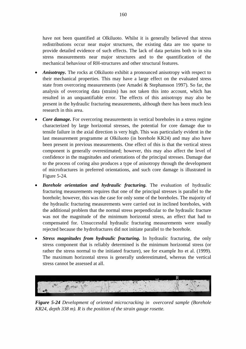
• Core damage. For overcoring measurements in vertical boreholes in a stress regime characterized by large horizontal stresses, the potential for core damage due to tensile failure in the axial direction is very high. This was particularly evident in the last measurement programme at Olkiluoto (in borehole KR24) and may also have been present in previous measurements. One effect of this is that the vertical stress component is generally overestimated; however, this may also affect the level of confidence in the magnitudes and orientations of the principal stresses. Damage due to the process of coring also produces a type of anisotropy through the development of microfractures in preferred orientations, and such core damage is illustrated in Figure 5-24.

• Borehole orientation and hydraulic fracturing. The evaluation of hydraulic fracturing measurements requires that one of the principal stresses is parallel to the borehole; however, this was the case for only some of the boreholes. The majority of the hydraulic fracturing measurements were carried out in inclined boreholes, with the additional problem that the normal stress perpendicular to the hydraulic fracture was not the magnitude of the minimum horizontal stress, an effect that had to compensated for. Unsuccessful hydraulic fracturing measurements were usually rejected because the hydrofractures did not initiate parallel to the borehole.

• Stress magnitudes from hydraulic fracturing. In hydraulic fracturing, the only stress component that is reliably determined is the minimum horizontal stress (or rather the stress normal to the initiated fracture), see for example Ito et al. (1999). The maximum horizontal stress is generally underestimated, whereas the vertical stress cannot be assessed at all.

Figure 5-24 Development of oriented microcracking in overcored sample (Borehole KR24, depth 338 m). R is the position of the strain gauge rosette.

161

In conclusion, the dispersion in the stress data at Olkiluoto is typical for the methods used. The most significant uncertainties that affect the results are the anisotropy of the rock, core damage and the presence of major fracture zones. Based on these findings, it is estimated that the absolute error in the stress magnitudes obtained could be as high as 5 MPa, whereas stress orientations could have an error of 30° or more in specific cases. However, for individual measurements the scatter can be larger than these values — up to 10 MPa in magnitude, 90° in trend and 30° in plunge, with the largest scatter in stress orientations being observed for the overcoring results.

It should be emphasized that none of the stress measurements at Olkiluoto has been carried out under the conditions assumed for the application of the methods. The most significant problem appears to be the pronounced anisotropy at the site and a reduction in uncertainty can, therefore, only be achieved via an improved interpretation method that account for anisotropy. Once this is in place, it should be possible to account for the effects of, for example, brittle deformation zones.

5.5.2 Uncertainties in the intact rock properties A relatively large number of samples of mica gneiss migmatite have been tested, in comparison with the other rock types where few tests have been carried out. Point load index tests conducted in the field indicate, however, that there are no large differences in properties between mica gneiss migmatite and the other gneissic rock types.

The clear anisotropy in the deformation and strength properties of the mica gneiss migmatite, which is related to the presence of the gneissic banding, has been studied only in recent tests. The deviation of the results is still considerable, but an additional problem is that, because of the small diameter of the deep boreholes, it has not been possible to obtain samples for testing at all orientations to the anisotropy. In particular, the most critical angles of 0 and 90 degrees are currently missing. The anisotropy of the other main rock types has not yet been studied, nor has the effect of the gneissic banding on other properties of the mica gneiss migmatite.

The effect of this anisotropy needs to be studied, and samples will be most easily obtained from the ONKALO access tunnel. The orientation of the sampling borehole with respect to the gneissic banding can be selected, as required, and samples from effectively the same location with different orientations can then be obtained.

It should be noted that parameters in rock mechanics, such as the strength and deformation properties of rock, the inclination and orientation of fractures in a rock mass and the measured in situ stresses do not have any single fixed value, but assume a wide range of values and are spatially variable in a crystalline rock mass. These variations are defined by a set of variables that describe the range of parameter values observed or expected and there is no way of predicting exactly what the value of one of these parameters will be at any given location.

The strength properties of the rocks, as described above, are an example of a property which is spatialy variable due to the heterogeneity of the rock mass. However, probability functions are able to indicate the relative likelihood that an essentially

162

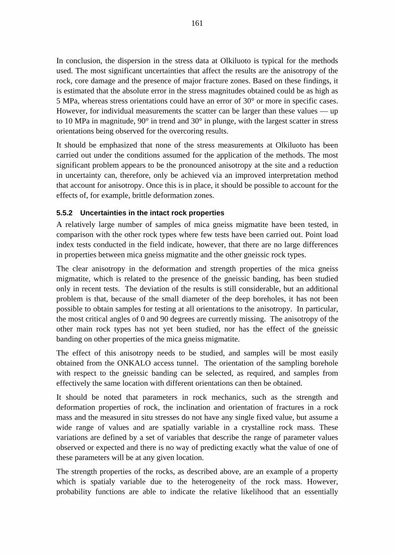
unknown variable will assume a particular value at a specified location. There are several ways of presenting this probability. If the distributions of properties are normal (or log-normal), the mean values and their standard deviations should be chosen to characterise the distribution. On the other hand, if the distributions of properties are skewed at different sites, if one test result departs significantly from other results, or if there are too few test values, it is sometimes better to choose median values and their quartiles, because these are independent of the nature of the distributions. An example on the strength distributions is shown in Figure 5-25.

Olkiluoto Mica gneiss - Peak strength (UCS), 59 samples

Laboratory testData from Johansson & Rautakorpi 2000

0

5

10

15

20

25

30

35

40

<50 50-75 75-100 100-125 125-150 150-175 175-200

Peak strength [MPa]

Freq

-%

Median 106,4 MPaMean 106,3 MPa

Mica gneiss - point load test, 446 samples

Data from Pohjanperä et al 2004

0

5

10

15

20

25

30

35

<50 50-75 75-100 100-125 125-150 150-175 175-200 200-225 225-250

Peak strength [MPa]

Freq

-%

Median 116 MPaMean 117 MPa

Figure 5-25 Use of probability distribution to characterize the variation in rock strength based on lab tests (upper) and field tests (lower).

5.5.3 Uncertainties in physical properties The majority of physical property tests are reliable and certain. However, during the testing, the system used to define P-wave velocity was found to be unreliable and the determination of travel time was subjective. This led to a relatively high deviation of ±10%. The average P-wave velocity is 4446 m/s.

163

5.5.4 Uncertainties relating to thermal properties The values in Table 5-7 are for intact rock as measured in the laboratory and there is the question as to how these values should be upscaled for use at the scale of the rock mass. Values for intact rock were obtained in the range 2.41 to 4.23 W/mK, which is in good agreement with the theoretical values estimated from their mineralogical compositions. The scatter in results is partly due to the anisotropy and this subject will require more consideration in the future. In addition, in situ tests will be carried out to provide more information on the scale effects.

5.5.5 Uncertainties related to fracture mechanical properties There is an overall uncertainty due to a lack of data on the mechanical properties of fractures. This situation will be rectified, at least in part, when the existing boreholes are re-logged and the fracture information is re-analyzed, taking into account the supporting geological information. Also, new samples of fractures at larger scales will become available from the ONKALO.

5.5.6 Uncertainties related to brittle deformation zone properties As with the individual fractures, there is an overall uncertainty due to the lack of comprehensive data – in this case relating not only to the mechanical properties but also to the geometry of the cluster of individual fractures which make up a fracture zone. A photographic record has been made of the fracture zones as they occur in the cores which gives some indication of their nature. However, there will be an opportunity to study some zones in detail in situ when they are intersected by the ONKALO access ramp.

5.5.7 Uncertainties related to rock mass properties No detailed analysis of the variation of dynamic elastic moduli with depth, rock type, fracture density, etc. has been carried out. A reliable knowledge of the distribution of these parameters would require accurate depth matching of the logging data, and the use of detailed core or image logging data, as the existing presentation of the core logging data is not sufficiently detailed.

Uncertainties, other than those related to the scale and representativity of specimens, are related to the direction of the measurements. Acoustic borehole logging measures P- and S-wave velocities in the direction of the borehole axis, and the velocity determined is an interval value over a distance of 40-100 cm along the borehole, which is related to the separation of the transmitter and the receiver. In a transversely isotropic medium, the velocities are highest when measured parallel to the foliation and lowest normal to the foliation; and the same behaviour is seen with the rock mechanics parameters. The intersection angle of the borehole to the foliation within the rock will, therefore, affect the magnitude of the results.

5.5.8 Evaluation of uncertainties relating to microseismic measurements The identification of an individual event among the cluster of blasts from the tunnelling activities includes elements of uncertainty. The majority of the excavation-induced

164

seismicity events tend to occur very close, in time and space, to the latest blast (Type A). These events often occur in swarms and their seismic signals do not represent a typical earthquake signal; they are associated with “fracture-dominated” rupture. Type B events are temporally and spatially distributed throughout the active excavation region. They represent “friction-dominated” slip in existing shear and fracture zones and have source properties similar to tectonic earthquakes (Richardson & Jordan, 2002). Type B events have many characteristics that make them easier to identify in comparison with type A events.

The accurate location of a seismic event is one of the key parameters for seismological interpretation; if the location is incorrect, the subsequent seismological analysis is inaccurate. Continuous calibration of the seismic velocity model is, therefore, required during the course of the excavation of the ONKALO.

165

6 HYDROGEOLOGY AND HYDROGEOCHEMISTRY

6.1 Background The hydrogeological model includes the concept of present-day groundwater compositions and flow as well as the palaeohydrogeological evolution of Olkiluoto. The science of palaeohydrogeology aims at understanding the past conditions that have determined the movements and compositions of groundwaters (e.g. Bath et al. 2000). The time intervals of interest in palaeohydrogeology can include the short timescales of anthropogenic influence and the very long timescales of geological processes; with the focus of the present study being on a timescale of up to about 10 000 years. This timescale is of interest, as it makes use of information which it is possible to apply with a fairly high level of confidence.

The simulation of groundwater flow over a period in the past introduces a challenge that tests our understanding of the site-scale hydrogeological flow concept (Bath and Lalieux 1999). Hydrogeochemical information may provide a means of improving the credibility of the site-scale groundwater flow model. This approach may be useful over this period of time, because conservative hydrogeochemical parameters in particular contain a record of cumulative changes. The degree of progressive mixing between water masses is a characteristic of groundwater movement, which is exposed more clearly in hydrochemistry than is possible from physical measurements alone.

The boundary conditions for the palaeohydrogeological evolution of the site can be determined from an understanding of recent geological history (since the Weichselian glaciation), which can be supplemented and made more precise by the use of hydrogeochemical information. Assessing groundwater flow simulations with hydrogeochemical data and comparing the temporal results of flow simulations with the corresponding interpretation of hydrogeochemical conditions, provides an iterative process for achieving a consistent interdisciplinary model of the site. Integration provides an opportunity to improve our understanding of the hydrogeological performance of the site and to increase confidence regarding future predictions of its hydrogeochemical evolution, which is essential to the development of the safety case.

Based on earlier groundwater geochemical studies (e.g. Pitkänen et al. 1994, 1996, 1999a, b, 2004) it is clear that the Holocene history of the Baltic Sea, in particular, has had a major effect on groundwater compositions at Olkiluoto. These studies presented the ages of post-glacial stages as radiocarbon years (uncalibrated ages) before present (BP), which are, however, shorter than calendar years, especially when considering times close to the Weichselian glaciation, due to the higher radiocarbon content in the atmosphere than in 1950 (year 0 in radiocarbon dating) (e.g. see Clark and Fritz 1997). Therefore, the time period since the Weichselian glaciation is summarised here using dates calibrated to calendar years, which are presented, for example, in Salonen et al. (2002).

166

Complete Weichselian deglaciation started about 11 500 years ago, and soon after that Olkiluoto was released from the cover of ice (about 11 000 years ago), but remained below the surface of the mildly saline Yoldia sea (Eronen & Lehtinen 1996) (Figure 6-1). The Olkiluoto site also remained submerged during the stages of the fresh Ancylus Lake (starting some 10 800 years ago) and the saline Litorina Sea (starting around 8 500–8 000 years ago) (Figure 6-1). During the main part of the Litorina stage, between about 8 000 and 4 500 years ago, the TDS in the seawater was about 4‰ higher than in the modern Baltic Sea at the Finnish coast (Donner et al. 1999). Since that time the salinity of the seawater has been reduced steadily to its current value of about 6‰ off Olkiluoto Island. As a result of land uplift Olkiluoto Island begun to emerge from the Baltic Sea about 3 000–2 500 years ago (Eronen & Lehtinen 1996). Currently the post-glacial uplift at the site is about 4–6 mm/yr (Eronen et al. 1995, Kakkuri 1987). From a hydrogeological viewpoint, there are two important salinity variations, firstly those in the Baltic Basin, and secondly the salinity (i.e. density) differences in the groundwater.

Figure 6-1. Postglacial shoreline in southern Finland from about 11 500 years ago until present (after Eronen et al. 1995, Pitkänen et al. 2004). Table 6-1 presents estimates of the compositions of glacial meltwater during the Weichselian deglaciation and of Litorina seawater; the latter estimate is based on the compositions of modern sea waters. The estimates for the compositions of present Baltic Sea and mean global ocean water are for surficial seawaters.

167

Table 6-1. Estimated Quaternary glacial meltwater and Litorina seawater compositions with inferred Baltic sea and mean ocean water compositions (Pitkänen et al. 1999).

1)Glacial water

2)Litorina sea

3)Baltic sea

4)Ocean water

T (°C) 1.0 10.9 8.5 20.0O2 (mg/l) 7.2 6.6 7.2 4.3pH 5.8 7.6 7.7 7.5Density (g/ml) 1.000 1.008 1.002 1.030HCO3 (mg/l) 0.16 92.5 78.7 144.2SO4 (mg/l) 0.05 890 450 2540PO4 (mg/l) 0.0003 0.06 0.02 0.22Ntot (mg/l) 0.19 0.27 0.21 0.5Cl (mg/l) 0.70 6500 3025 19550F (mg/l) 0.00 0.49 0.27 1.3Br (mg/l) 0.001 22.2 10.3 67NO3 (mg/l) 0.07SiO2 (mg/l) 0.01 1.84 0.58 6.61Fetot (mg/l) 0.0001 0.002 <0.01 0.002Al (mg/l) 0.0001 0.002 <0.01 0.002Na (mg/l) 0.15 3674 1760 10860K (mg/l) 0.15 134 66 391Ca (mg/l) 0.13 151 82 412Mg (mg/l) 0.1 448 219 1310Mn (mg/l) 0.0 0.0 <0.01 0.0Sr (mg/l) 0.0001 2.68 1.20 8.24Li (mg/l) 0.0 0.07 0.04 0.18Charge Balance (%) 1.03 0.97 2.13 0.27δ2H (o/oo SMOW) -166.0 -37.8 -60.8 -30.0δ13C (PDB) -25.0 -1.0 -1.68 -1.0δ18O (o/oo SMOW) -22.0 -4.7 -7.55 -4.03H (TU) 0.0 0.0 15.4 15.414C (pM) 28.0 43.0 115.8 10087Sr/86Sr 0.70940 0.70945 0.7094

1) pH, Na, K, and SO4 values estimated from Taylor et al. (1992). δ18O and δ2H values are discussed in section 6.1.3. 14C value is based on conservative isotopic decay and δ13C value indicates organogenic origin of carbon. 2) Regression between average Baltic sea (Puskakari, Eteläriutta) and global mean ocean water (Fairbridge 1972, Harrison 1992) with assumption that maximum Cl-content in Litorina sea has been about 6500 mg/l (Kankainen 1986). 14C value is based on conservative isotopic decay. 3) Average of ’94 samples from Puskakari and Eteläriutta. 4) Global mean ocean water (Fairbridge 1972, Harrison 1992).

168

The hydrogeochemical evolutionary concept for Olkiluoto since the start of the Litorina stage was adapted from the prevailing hydrogeological model (Löfman 1999) as part of the international EQUIP project (Bath et al. 2000, Gehör et al. 2002). Hydrogeological modelling was able to apply temporal salinity (density) variations in the boundary conditions of the flow simulations and to examine salinity changes in groundwater at Olkiluoto from the Litorina stage up to the present-day. The temporal correspondence between the hydrogeochemical results and the simulated evolution of the salinity was not optimum, particularly in the upper 300 m of the bedrock, where groundwater at the end of the simulations was clearly more diluted than that observed in groundwater samples or in borehole measurements of electrical conductivity (EC). No adjustments were made to the hydrogeological properties of the bedrock, in order to obtain a better correspondence between the disciplines, because the concept of baseline conditions was then under development and the characterisation of the hydrogeological and chemical conditions was incomplete. The database and the characterisation of baseline conditions are currently almost complete, therefore, allowing a more thorough integration effort to be attempted.

6.2 Conceptual Models

6.2.1 Hydrogeological model The interpretations based on geological, hydrological and geochemical field investigations have been used in the selection and development of a modelling approach for numerical groundwater flow simulations, and in the determination of initial and boundary conditions. Due to variations in the density of groundwater, the simulations call for coupled modelling of flow, and solute transport and transient analyses are required because of the evolving hydraulic conditions.

6.2.1.1 Modelling fractured rock The crystalline bedrock consists of solid rock cut by a network of fractures (Figure 6-2). Water flows primarily along an intricate network of paths formed by a small portion of interconnected fractures (water-bearing fractures), whilst most of the fractures and other volumes of rock with low fracture density (matrix blocks) contain essentially stagnant water. The hydraulic characteristics of the rock are mainly defined by the properties of the fracture network, i.e. the permeability, density, size and orientation distributions of the fractures. The transport of saline groundwater in the fractured system is accompanied by the diffusion of solute particles from fractures, containing mobile water, to matrix blocks, and vice versa, i.e. the matrix blocks act as sources (and/or sinks) that feed (and/or drain) the water-bearing fractures. This diffusion process is called matrix diffusion and may constitute a process that can be effective in retarding transport through the system. In this study, the hydraulic characteristics of fractured rock mass are modelled conceptually with two alternative approaches: the equivalent-continuum (EC) and the

169

dual-porosity (DP) approach (Löfman 2000). In the EC model (Figure 6-2) the fractured system is treated as a homogeneous continuum with representative, averaged hydraulic characteristics. No distinction is made between fractures and matrix blocks, but water is assumed to flow through the whole system. The EC approach is commonly used in representing the fractured bedrock. However, although the EC approximation may be valid from the standpoint of flow, it becomes more restrictive when transport phenomena are also considered, because it cannot take into account, for example, the retardation effect of matrix diffusion. Thus, a more realistic DP approach is also employed in this study. In the DP model (Figure 6-2), the system is assumed to consist of two overlapping continua: the fractures with flowing water and the matrix blocks with essentially stagnant water, representing the rest of a system. The convection and dispersion are the dominant processes within the water-bearing fractures, whereas molecular diffusion is the dominant process in the matrix blocks. Thus, with the DP approximation the retardation effect caused by the matrix diffusion of solutes from the rock blocks containing stagnant water can be considered. From the point of view of groundwater flow, matrix and fractures are approximated to be in pressure equilibrium and the matrix blocks are ignored in the simulations. The modelled bedrock volume is conceptually divided into hydrogeological units: planar fracture zones (the parts of the bedrock with a higher fracture density and a greater ability to conduct water) and sparsely fractured rock between the zones (the remaining part of the bedrock, in which fracture density and conductivity is lower). The EC and DP concepts are applied separately for each hydrogeological unit.

Figure 6-2. A schematic description of the real bedrock (left) with its equivalent-continuum (EC) (middle) and dual-porosity (DP) (right) representations.

170

6.2.1.2 Modelled volume The size of the modelled bedrock volume is about 25 km2 horizontally and 2 km in depth (Figure 6-3). The modelled area covers the Olkiluoto Island in such a way that the distance of the vertical boundaries from the present shoreline is about 200-1000 m and from the ONKALO about 2-3 km. As the ONKALO and the repository extend to a maximum depth of about 500 m, the locations of the vertical and bottom boundaries can be assumed to be far enough from the area of primary interest to make the effects of the uncertainty associated with the boundary conditions insignificant.

Figure 6-3. Modelled volume and well characterised area (WCA, dashed rectangular).

6.2.1.3 Bedrock model The bedrock model of the Olkiluoto site was updated during spring 2003 (Vaittinen et al. 2003). In the present model, 96 fractured structures are described in the structural model and 75 hydraulically important structures in the hydrogeological model. A subset of 26 structures is common to both models and the total number of directly-observed

171

structures is 145. The naming convention of structures has been changed to show the model category. The descriptive attribute ‘R’ refers to objects in the structural model and the attribute ‘H’ to those in the hydrogeological model of Vaittinen et al (2003).

In the present version fracture frequency, hydraulic conductivity and mapped fracturing class are the defining parameters for structural intersections in boreholes. The fracturing class (Ri-value) is based on the Finnish engineering geological classifications and the class describes the type of structural intersection, whereby Ri III corresponds to ‘fracture zone’ and Ri IV - Ri V correspond to ‘crushed zone’. If the bedrock is averagely fractured and the hydraulic criterion is fulfilled, the structure is referred to as a ‘hydraulic feature’.

The orientation of structures is mainly based on oriented fractures, determined either from core samples or from optical borehole images. In addition, seismic and borehole radar measurements are used to orientate some structures. Of the total of 145 structures, 40 structures are not oriented due to a lack of orientation data. The continuity of structures is assessed on the basis of geological properties, hydraulic responses, seismic measurements and galvanic charged potential measurements.

When directly-observed structures are taken into account, dip directions are concentrated in the range 140 - 180º, and dip angles in the range 0 - 50º, which is similar to the oriented fractures seen in boreholes. The thickness of these structures is typically a few metres: the average thickness is 6.2 m, but the median is only 3.6 m. The average transmissivity of the structure categories varies from 4·10-6 m2/s for hydraulic features to 5·10-8 m2/s for fracture zones; and about 20% of the structures are considered to have a transmissivity greater than 1·10-5 m2/s. Most of the structures, 126 in all, intersect only one borehole, 19 structures can be correlated either from one borehole to another or from a borehole to the ground surface.

6.2.1.4 Conceptual fracture zone geometry The geometry of the fracture zones is based on the hydrogeological model and on the correlated structures of the structural model of version 2003/1 of the Bedrock model (Vaittinen et al. 2003). Altogether the hydrogeological model and the structural model consist of 145 directly-observed fractured zones (R-structures) and/or features that are judged to be hydraulically important (RH/H-structures), even though they do not display signs of extensive and frequent fracturing (Vaittinen et al. 2003). Most of the structures in the bedrock model have been observed only in one borehole and are represented as discs (with a constant diameter of 100 metres) centred on the relevant boreholes. However, from the point of view of site-scale modelling of groundwater flow, such isolated disks, which do not intersect other zones and therefore do not constitute important flow routes, are irrelevant.

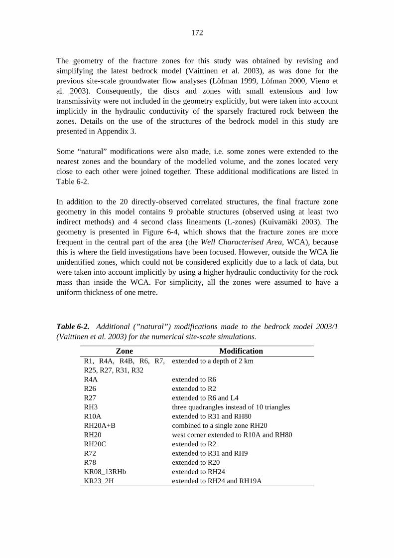
172

The geometry of the fracture zones for this study was obtained by revising and simplifying the latest bedrock model (Vaittinen et al. 2003), as was done for the previous site-scale groundwater flow analyses (Löfman 1999, Löfman 2000, Vieno et al. 2003). Consequently, the discs and zones with small extensions and low transmissivity were not included in the geometry explicitly, but were taken into account implicitly in the hydraulic conductivity of the sparsely fractured rock between the zones. Details on the use of the structures of the bedrock model in this study are presented in Appendix 3. Some “natural” modifications were also made, i.e. some zones were extended to the nearest zones and the boundary of the modelled volume, and the zones located very close to each other were joined together. These additional modifications are listed in Table 6-2. In addition to the 20 directly-observed correlated structures, the final fracture zone geometry in this model contains 9 probable structures (observed using at least two indirect methods) and 4 second class lineaments (L-zones) (Kuivamäki 2003). The geometry is presented in Figure 6-4, which shows that the fracture zones are more frequent in the central part of the area (the Well Characterised Area, WCA), because this is where the field investigations have been focused. However, outside the WCA lie unidentified zones, which could not be considered explicitly due to a lack of data, but were taken into account implicitly by using a higher hydraulic conductivity for the rock mass than inside the WCA. For simplicity, all the zones were assumed to have a uniform thickness of one metre.

Table 6-2. Additional (”natural”) modifications made to the bedrock model 2003/1 (Vaittinen et al. 2003) for the numerical site-scale simulations.

Zone Modification R1, R4A, R4B, R6, R7, R25, R27, R31, R32

extended to a depth of 2 km

R4A extended to R6 R26 extended to R2 R27 extended to R6 and L4 RH3 three quadrangles instead of 10 triangles R10A extended to R31 and RH80 RH20A+B combined to a single zone RH20 RH20 west corner extended to R10A and RH80 RH20C extended to R2 R72 extended to R31 and RH9 R78 extended to R20 KR08_13RHb extended to RH24 KR23_2H extended to RH24 and RH19A

173

Figure 6-4. Modelled bedrock volume and conceptual fracture zone geometry based on the bedrock model 2003/1 (Vaittinen et al. 2003).

6.2.2 Hydrogeochemical model

The interpretation of the hydrogeochemical evolution of Olkiluoto is based on chemical and isotopic data of water samples (c.f. Chapter 2) and minerals, and on geochemical modelling, in conjunction with a knowledge of the hydrogeology and geology of the site. The status of interpretation is composed of several issues important for site understanding and for evaluating the long-term safety of the repository, i.e. predictions as to the future evolution of the site. Such issues will include the origin of groundwaters, the residence time for groundwaters (the flow dynamics of the site), hydrogeochemical influences of palaeoenvironmental changes (e.g. glaciation, marine stages, etc.), the influence of water-rock interactions, pH and redox buffering processes and their capacity, i.e. the hydrogeochemical stability of the groundwater system in response to natural disturbances. Geochemical modelling is an important exercise for increasing the level of understanding of hydrogeochemical evolution and hydrogeology, by providing information on the extent of mass transfer in plausible chemical reactions,

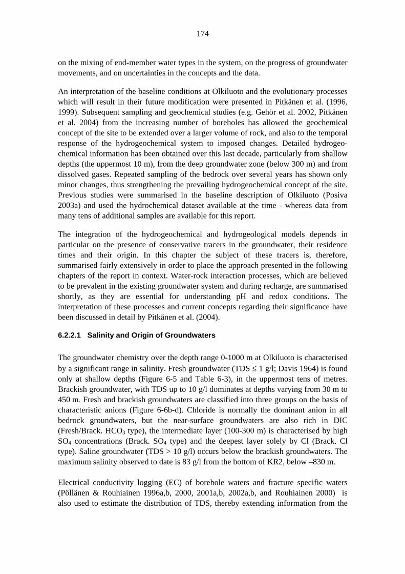
174

on the mixing of end-member water types in the system, on the progress of groundwater movements, and on uncertainties in the concepts and the data.

An interpretation of the baseline conditions at Olkiluoto and the evolutionary processes which will result in their future modification were presented in Pitkänen et al. (1996, 1999). Subsequent sampling and geochemical studies (e.g. Gehör et al. 2002, Pitkänen et al. 2004) from the increasing number of boreholes has allowed the geochemical concept of the site to be extended over a larger volume of rock, and also to the temporal response of the hydrogeochemical system to imposed changes. Detailed hydrogeo-chemical information has been obtained over this last decade, particularly from shallow depths (the uppermost 10 m), from the deep groundwater zone (below 300 m) and from dissolved gases. Repeated sampling of the bedrock over several years has shown only minor changes, thus strengthening the prevailing hydrogeochemical concept of the site. Previous studies were summarised in the baseline description of Olkiluoto (Posiva 2003a) and used the hydrochemical dataset available at the time - whereas data from many tens of additional samples are available for this report.

The integration of the hydrogeochemical and hydrogeological models depends in particular on the presence of conservative tracers in the groundwater, their residence times and their origin. In this chapter the subject of these tracers is, therefore, summarised fairly extensively in order to place the approach presented in the following chapters of the report in context. Water-rock interaction processes, which are believed to be prevalent in the existing groundwater system and during recharge, are summarised shortly, as they are essential for understanding pH and redox conditions. The interpretation of these processes and current concepts regarding their significance have been discussed in detail by Pitkänen et al. (2004).

6.2.2.1 Salinity and Origin of Groundwaters The groundwater chemistry over the depth range 0-1000 m at Olkiluoto is characterised by a significant range in salinity. Fresh groundwater (TDS ≤ 1 g/l; Davis 1964) is found only at shallow depths (Figure 6-5 and Table 6-3), in the uppermost tens of metres. Brackish groundwater, with TDS up to 10 g/l dominates at depths varying from 30 m to 450 m. Fresh and brackish groundwaters are classified into three groups on the basis of characteristic anions (Figure 6-6b-d). Chloride is normally the dominant anion in all bedrock groundwaters, but the near-surface groundwaters are also rich in DIC (Fresh/Brack. HCO3 type), the intermediate layer (100-300 m) is characterised by high SO4 concentrations (Brack. SO4 type) and the deepest layer solely by Cl (Brack. Cl type). Saline groundwater (TDS > 10 g/l) occurs below the brackish groundwaters. The maximum salinity observed to date is 83 g/l from the bottom of KR2, below –830 m. Electrical conductivity logging (EC) of borehole waters and fracture specific waters (Pöllänen & Rouhiainen 1996a,b, 2000, 2001a,b, 2002a,b, and Rouhiainen 2000) is also used to estimate the distribution of TDS, thereby extending information from the

175

geochemical sampling data. The results between EC measurements and hydrochemical data (Figure 6-6a) are in fairly good agreement, thereby increasing the reliability of the hydrochemical data (Pitkänen et al. 2004). Significant deviations are observed in the data from borehole KR12, where EC values from wireline logging clearly exceed conductivities measured from groundwater samples. The difference may result from the method of EC logging, in which the whole borehole is pumped from its upper part during measurements. Highly saline water, discharged from a transmissive fracture zone at depth in the borehole, may have disturbed fracture EC logging. The salinity of groundwater samples from borehole KR12 corresponds well with the hydrochemical data from similar depths in the other boreholes, providing support for the reliability of groundwater samples. The interdependence between salinity and hydraulic conductivity seems to be relatively indistinct (Figure 6-6b). Brackish and saline groundwaters do not show any trend with hydraulic conductivity, whereas the salinity seems to increase in HCO3-rich groundwater with decreasing conductivity. However the latter dependence may also be due to independent factors. Hydraulic conductivity decreases generally in the upper 150 m (see Section 6.3.2) and salinity enrichment is caused by mixing between meteoric infiltration and SO4-rich brackish groundwater. This may indicate that salinity enrichment is mainly controlled by factors other than the transmissivity of fractures and deformation zones. A large salinity variation itself may buffer lighter and less saline water circulation, even in strongly transmissive zones. The result of this buffering may be that groundwater types form a fairly smooth, layered structure, something that is also suggested in Figure 6-5, where water types change with depth at a scale of tens rather than hundreds of metres. The hydrochemical data have revealed the complex nature of the sources of salinity and groundwater evolution at Olkiluoto (Pitkänen et al. 1996, 1999, 2004). Changes in climate and geological environment have had a significant effect on local palaeohydrogeological conditions, and have left clear imprints on chemical and isotopic signatures, which are, for example, reflected in the characteristic anion contents. As a consequence of these changes, the current groundwater compositions and the chemical data show a great variability with depth (Figure 6-5 and Table 6-3), notably in salinity, as do the water types and the relative contents of conservative tracers such as Cl, Br, δ2H and δ18O (Figure 6-7). Hydrochemical data have also revealed the extensive mixing phenomena of different end-member waters from each of the palaeo sources.

176

Figure 6-5. a) TDS, b)Cl, c) DIC and d) SO4 as a function of depth of Olkiluoto. Baltic seawater has been sampled offshore Olkiluoto.

177

Figure 6-6 a) Relationship between EC results from groundwater samples and flow logging measurements from corresponding specific fractures, b) TDS and corresponding hydraulic conductivity of sampling sections. Class 1 and 2 in a) refers to quality evaluation of groundwater samples (see chapter 2) representing quantitatively and qualitatively accepted samples, respectively.

178

The quality evaluation of the data for stable isotopic compositions of groundwater has been particularly thorough (see Chapter 2 and Hellä et al. 2005) and the evaluation of hydrochemical and isotopic data has clarified the interrelationships and distributions of stable isotopic compositions of groundwater types. The position of stable isotope compositions relative to the global meteoric waterline (GMWL) indicates potential chemical and physical conditions and processes (e.g. Clark & Fritz 1997, Frape et al. 2004), which are indicated in the Figure 6-7a. The isotopic composition of groundwater is in most cases controlled by meteorological processes and the shift along the GMWL reflects climatic changes in precipitation. Cold climate precipitation shows lighter isotopic composition (more negative values), whereas warmer climate shows heavier composition. A shift to the right or below the GMWL typically indicates evaporation in surficial waters, which are enriched due to fractionation in heavier isotopes, particularly 18O, relative to formed vapour. Therefore, seawater composition is, for example, below the GMWL. The shift above the GMWL is unusual and observed mainly in shield brines. In order to produce such strong fractionation in oxygen and hydrogen isotopes, it has been proposed that this is due to effective primary silicate hydration under a low water-rock ratio (see discussion below). The stable isotopic data for the groundwater at Olkiluoto reveal five extreme compositions (Figure 6-7). They are: 1) current recharge which plots over a limited area along the GMWL, 2) seawater that has a signature which shows evaporative effects (brackish SO4 type also tends to shift towards seawater), 3) water from the Korvensuo reservoir (domestic water used in drilling - originally river water) showing an even stronger evaporative tendency than seawater, 4) meteoric water (brackish Cl type) that shows a colder climate signature, and finally 5) the signature in saline groundwater above the GMWL, which indicates strong hydration of silicates. The interpretation of chemical and isotopic data indicates, however, that there are at least six end-member water types influencing current groundwater compositions at the site. They originate from different periods, ranging from modern times, through former Baltic stages to preglacial times: modern - meteoric water that infiltrated during terrestrial recharge, - water infiltrated from the Korvensuo reservoir and - seawater from the Gulf of Bothnia (0 – 2 500 BP) relic - Litorina Sea water (2 500 – 8 500 BP)

- fresh water prior to the Litorina Sea stage containing glacial meltwater (8 500 – 11 000 BP) and

- saline water (brine) intruded and/or formed under the influence of hydrothermal activity (pre-Quaternary, probably early Phanerozoic to Precambrian in age).

179

Groundwater representing modern water types occurs in the upper 100 – 150 m (Table 6-3). The latest stage of groundwater formation is dominated by dilute carbonate-rich infiltration, with stable isotopic signatures of water, corresponding to current, dilute meteoric recharge at shallow depths in soil and bedrock. Carbon isotopes of DIC and isotopic calculations (Pitkänen et al. 1999, 2004) indicate that its high carbonate content is due to recent respiration of organic matter and to the dissolution of calcite. Seawater input is indicated by increasing salinity, seawater signatures of Br/Cl (Figure 6-7) and Na/Ca ratios, and increasing SO4 and Mg contents with marine Cl-ratios (Pitkänen et al. 1996, 1999, 2004). The influence of the Korvensuo reservoir is observed in its neighbourhood, in stable isotopic composition in a few groundwater samples taken from overburden and shallow bedrock (Figure 6-7). Its chemical composition is similar to corresponding shallow groundwaters. The HCO3-rich groundwater type has been formed since Olkiluoto Island rose above sea level about 2500 years ago, but the general observation of tritium and moderate radiocarbon values (50 - 60 pM or higher), which, due to isotopic dilution, represent a modern range, indicate mostly recent recharge in the last few decades. Table 6-3. Vertical variation of the main hydrochemical parameters and microbes at Olkiluoto shown against indicative depth ranges. Variation in pH corresponds with calcite equilibrium in groundwaters and follows the variation in carbonate and calcium contents. Vertical lines in redox column depict steady conditions.

Depth (m)

Used classification

Water type Cl (mg/l) pH Alkalinity (meq/l)

Redox

0 Fresh HCO3 Ca-Na-Mg-HCO3 -SO4

<10 5.5 <0.5 Post-oxic

10 Ca-Na-Mg-HCO3 -(SO4-Cl)

10 7 3 Sulphidic

150 Brackish HCO3 Na-(Ca)-Cl-(HCO3 -SO4)

2000 7.8 4

200 Brackish SO4 Na-(Ca)-Cl-(SO4) 4500 7.5 1.0

Brackish Cl Na-Cl 2700 8.2 0.4 Methanic

450 Saline Na-Ca-Cl 8000 8 0.2

600 Ca-Na-Cl

14000 7.8

1000

45000 7.5 <0.1

The near-surface part of the bedrock, which is characterised by HCO3-rich groundwater, therefore appears to be hydraulically dynamic. Although the HCO3-rich groundwater has been recharged recently, 14C (35-45 pM) and 3H evaluations (Pitkänen et al. 2004)

180

suggest that the deeper, more saline samples of this near-surface zone have a mean residence time of over 500 - 3000 years. The distinctly SO4-rich brackish water below the HCO3-rich groundwater at 100 to 300 m depth (Figure 6-5 and Table 6-3) most probably infiltrated during the Litorina Sea stage (Pitkänen et al. 1996), when the island was still submerged. The marine origin of the water and the dissolved solids is indicated by the Br/Cl (Figure 6-7), SO4/Cl and Mg/Cl ratios, which are typical of seawater, a lower pH and alkalinity and much higher SO4 and Mg than in the HCO3-rich groundwater, and also by the trend of stable isotope composition of water towards Baltic composition (Figure 6-7). The higher Cl content than in modern Baltic water (3200 mg/l) is consistent with the estimates presented for the Litorina Sea (e.g. Kankainen 1986, Donner et al. 1999). The 14C content of dissolved carbonate (20 – 30 pM) corresponds to the Litorina Sea stage, in comparison with more recently recharged HCO3-rich groundwater (Pitkänen et al. 2004). Other evidence for seawater intrusion is provided by the marine signature in δ34S(SO4) (Pitkänen et al. 2004) and the observation by Gascoyne (2001) that these groundwaters all have low 36Cl/Cl ratios, which are comparable to modern Baltic seawater, and contrast with freshwater recharge and the deeper saline waters. The interpretation of glacial meltwater input is based on the decreasing stable isotopic values of SO4-rich groundwaters (Figure 6-7) and their low, meteoric signature in the lower part of the brackish layer in SO4-poor groundwaters, i.e. brackish, Cl-type groundwater. Salinity shows a slight decrease (Figure 6-5), and radiocarbon (4 – 25 pM) indicates ages corresponding to deglaciation or to the last glacial period in relation to the Litorina-derived groundwater. The chemical composition of brackish, Cl-type groundwaters shows a loss of its seawater signature - sulphate disappears and the Br/Cl ratio increases - suggesting a source of dissolved solids other than seawater and the possible input of HCO3-rich groundwater. The initial source is considered to be the same as for the saline water, i.e. ancient brine. High levels of dissolved hydrocarbons, notably CH4, also provide a connection between these DIC and SO4-poor groundwaters. Groundwater salinity starts to increase significantly at -300 to -400 m depth, without showing any indication of levelling off (Figure 6-5) or showing any discontinuity in the main chemical variables (Pitkänen et al. 1999, 2004). Calcium becomes the dominant cation, the Br/Cl ratio (Figure 6-7) reaches twice the level of seawater, and the stable isotopes of water show a positive trend with increasing salinity, shifting further above the GMWL. The original shift of brine composition above the GMWL is probably caused by the fractionation of stable isotopes during the hydration of silicates, e.g. the alteration of primary silicates, such as plagioclase, to clay minerals:

Na0.8Ca0.2Al1.2Si2.8O8 + 1.2 H+ + 0.6 H2O → 0.8 Na+ + 0.2Ca2+ + 0.6Al2Si2O5(OH)4 + 1.6 SiO2

181

Isotopic fractionation between the fluid and the crystallising clay mineral (kaolinite in the equation) partitions 18O into the mineral, thus depleting 18O in the residual fluid. The reverse occurs for hydrogen, and the residual fluid is thereby enriched in deuterium (e.g. Clark & Fritz 1997). Fractionation needs a very low water-rock ratio and occurs over geological time scales.

The origin of shield brines has been debated over several decades (e.g. Clark and Fritz 1997, Frape et al. 2004). The theories vary between an allocthonous fluid (e.g. seawater - evaporative seawater), which has moved to its present location, and an in situ origin, due to the development of increasing salinity during the hydration reactions of silicates which consume water. Recently a theory has been published (Starinsky and Katz 2003) that Fennoscandian brines have been formed by the freezing of seawater during Quaternary glaciations along the margins of continental ice sheets.

A similar chemical tendency to that of saline groundwater (Ca-Na-Cl) at Olkiluoto is observed in the highly saline (up to 30 wt.%) fluid inclusions in fracture calcites, which are formed at moderate to high temperatures (45 – 240˚C according to Blyth et al. 2000, Gehör et al. 2002). Abundant hydrocarbons in highly saline groundwater also display a mainly thermal source, which connects the origin of the brine component to hydrothermal conditions (Pitkänen et al. 2004). In situ 36Cl production in saline groundwater (Gascoyne 2001), in equilibrium with host production rates and U-series activity ratios which approach equilibrium, suggests a long residence time, on the million year scale. Indications from calcites, fluid inclusions, dominating hydrothermal wall rock alteration in fractures, dissolved gases and isotopic signatures in saline groundwater connect the formation of brine to hydrothermal conditions, and suggest an extremely early origin for the original brine end-member, which is impossible to relate to any well-known event during the Quaternary. Probably, the formation of the brine end-member occurred during the early Phanerozoic or late Precambrian, when the crust may have been covered by thick sediments, some of which are now preserved nearby in a graben to the north of the site and below the Gulf of Bothnia (Blyth et al. 2000, Pitkänen et al. 1999, 2004). Measured δ37Cl-values of about 0‰ from the most saline groundwaters suggest a seawater origin for chloride (Pitkänen et al. 2004). Thus the origin for brine may have elements of both the source processes discussed above - for example, evaporative, concentrated seawater that is modified by water-rock interaction in hydrothermal conditions.

182

Figure 6-7. Relationship between δ18O and δ2H (a) and Br-Cl ratio (b) in Olkiluoto groundwater samples. Arrows in a) depict to compositional changes caused by informed conditions. Global meteoric water line (GMWL) after Craig (1961). Note: no overburden samples included in the (b) part due to analytical uncertainties in very low Br contents.

183

6.2.2.2 Water-rock interaction Water-rock interaction, such as carbon and sulphur cycling and silicate reactions, buffer the pH and redox conditions (Figure 6-8) and stabilise groundwater chemistry at Olkiluoto. However, the extensive difference between the compositions of groundwater types also causes significant deviations in water-rock interaction processes, particularly in redox chemistry. Hydrogeochemical interpretations and chemical and isotopic calculations indicate that pH seems to be dominantly controlled by the thermodynamic equilibrium with calcite in fractures. Calcite is the most common fracture-filling mineral in the bedrock and there are indications that it may also occur in the soil layer. Thermodynamic calculations have presumed calcite equilibrium in groundwaters and suggest that the pH range varies from 7.5 in HCO3- and SO4-rich groundwaters, increasing to 8 in the lower part of brackish groundwaters, before decreasing again to 7.5 in saline groundwater. These calculated values are slightly less than measured values from groundwater samples (Pitkänen et al. 2004).

Oxic redox conditions in recharging groundwater change directly to sulphidic conditions close to the surface within a short residence time. The anaerobic reduction of sulphate with the oxidation of organic carbon seems to be the most important process governing the redox conditions in dilute and brackish HCO3-rich and SO4-rich groundwaters. Methanogenesis may show an increasing level of importance in saline groundwater and occasionally in brackish groundwater, below the SO4-rich layer. Haveman et al. (1998, 2000) have discovered microbes that are fundamental for these redox processes to occur in the groundwater at Olkiluoto. The results of equilibrium calculations indicate that the redox level decreases with depth from –200 mV to –250 mV in sulphidic redox conditions in brackish groundwaters, and further, to almost –300 mV in methanic systems, in the lower part of the brackish layer and in saline groundwaters (Pitkänen et al. 2004).

Mass-balance calculations performed by Pitkänen et al. (1999, 2004) suggest that, in current conditions or in sea bottom sediments during Litorina Sea state, the main mass transfer in reactions occurs at the few mmol level during infiltration, either in the overburden or in very shallow bedrock. At greater depth such mass transfer may be smaller, only some tenths of a mmol per kg of water. Organic carbon oxidation and calcite dissolution are the main reactions in the recharge zone, whereas bacterial SO4 reduction, with the oxidation of organic carbon causing pyrite and calcite precipitation, has dominated during the infiltration from the Litorina Sea. In addition, ion exchange and silicate dissolution are probable, but uncertainties in the data limit the potential for specifying the extent of mass transfer in these processes and its contribution to pH buffering. These processes need further examinations with forward geochemical modelling tools such as PHREEQC.

184

Figure 6-8. Illustrated west-east cross-section of hydrogeochemical and hydrogeological conditions in the bedrock of Olkiluoto, based on an interpretation of hydrogeochemistry (Pitkänen et al. 2004). Changes in colour describe alteration in water type. Blue arrows represent flow directions. Rounded rectangles contain the main sources and sinks affecting pH and redox conditions. Generalised fracture zones (coded by R) are combined on the basis of bedrock models by Vaittinen et al. (2003).

Mass transfer in redox reactions seems to increase in the transition zone, from SO4-rich groundwaters to SO4-poor groundwaters containing substantial CH4 at 300 to 400 m depth. The estimated total reduction of SO4 is thought to be about 110 mg/l, corresponding to the formation of 40 mg/l of sulphide, of which a significant part has precipitated as pyrite. The greatest observed dissolved sulphide content is 12.4 mg/l. Bacterial methane formation is evident at depth, but insufficient isotopic data on both DIC and hydrocarbons limit the evaluation of its magnitude and its effect on the carbonate system. The data on hydrocarbons indicate that thermal processes are the principal source for the production of CH4 and other hydrocarbons. However, it is unclear whether these compounds are formed by thermal decomposition of organic

185

matter or by hydrothermal reactions between carbonate or graphite with H2 (Pitkänen et al. 2004).

6.3 Evaluation of information

6.3.1 Hydrogeochemical information The description of hydrogeochemical conditions and their distributions in the bedrock is not a straightforward task, because current groundwater types are the result of progressive mixings between various end-member water types (e.g. brine, glacial meltwater, seawater etc.) which represent some of the major events at the site during its geological history. Therefore, single conservative hydrogeochemical variables are ambiguous and they characterise only poorly the chemical conditions or evolutionary stage in different parts of the site. Characteristic combinations of conservative variables (stable isotopes of water, Cl, Br) have made it possible to recognise reference groundwater samples (most extreme groundwater compositions, e.g. Figure 6-7), which are related to the end-member water types or initial waters of selected geological time periods (Pitkänen et al. 1999, 2004).

The inverse geochemical modelling approach (mass-balance calculations) used is a competent means of interpreting hydrogeochemical evolution along a flow path, i.e. water-rock interaction and mixing of initial water types in the system (cf. Chapter 6.2.2). So the hydrogeochemical system makes it possible to describe the mixtures of initial water compositions and their distributions in different parts of the site. The progressive mixing between initial water types is characteristic of groundwater conditions and movements, that are more sensitively reflected in hydrogeochemical changes than could be interpreted from single measurements alone. In addition, the initial water types can usually be associated with known geological periods or events that provide a time frame to the groundwater flow. Progressive changes in water compositions in different parts of the site may also be used during the ONKALO construction phase, either as an initial reference for forward hydrogeological simulations, or as a final evaluation tool for various hydrogeological predictions (e.g. salinity predictions).

It is impossible to apply chemical steady-state conditions, which are essential for mass-balance calculations (Plummer et al. 1994), to the whole hydrogeochemical evolutionary path observed at Olkiluoto. If the interpreted end-member compositions were used directly, the results of calculations would represent the sum of many processes, some of which may have occurred over millions of years, e.g. the dilution of the brines. The time period to be modelled has to be well-defined and, in this case, the time since the Weichselian glaciation (cf. Figure 6-9) has been selected, in which deglaciation forms the initial stage, and has been modelled using the mass-balance method (Pitkänen et al. 1999, 2004, Luukkonen et al. 2005).

Geochemical modelling, as well as the modelling of the hydrogeological evolution, needs an evaluation of the initial salinity conditions in the bedrock and at the upper boundary throughout the simulations, i.e. the variation of seawater salinity. Current

186

groundwater samples are mixtures of ancient end-member water compositions, which represent formation waters from certain geological conditions, such as Litorina seawater, glacial meltwater and original brine. The groundwater data contain reference samples that are derivatives of those end-member waters. There have also been certain groundwaters representing intermediate stages, which occurred in the bedrock when hydrogeological conditions changed during deglaciation and postglacial times. For example, it is unlikely that marine infiltration from the Litorina Sea mixed with pure meltwater in the bedrock (Figure 6-9). This pre-Litorina groundwater was probably a mixture of infiltrated glacial meltwater and previous subglacial groundwater (initial water, for our mass-balance calculations that was modified during the glacial period) which, according to the salinity of the most extreme meltwater reference samples (TDS = 4 000 - 4 500 mg/l, Cl = 2 400-2 760 mg/l and no marine signature), had to be brackish to slightly saline in the upper part of the bedrock. In addition, the groundwater before Litorina infiltration probably had only a trace of SO4, if any, as indicated by the Cl-dominated brackish and saline groundwater types seen today.

Although SO4 does not conform completely to the requirement for conservatism, the salinity (or Cl content) of pre-Litorina and subglacial groundwater in the upper part of the Olkiluoto bedrock was estimated with the help of Cl, δ18O and SO4 data from Pitkänen et al. (1999). Comparison of δ18O and Cl data (Figure 6-10a) indicates four distinct reference groundwaters, which can govern the other groundwater compositions by mixing. The waters are meteoric, Litorina reference, glacial reference and brine reference which, with the addition of Baltic seawater (basically diluted Litorina), enables the mixing traces of the other samples to be determined. Because Litorina and glacial reference waters are not the original end-members, the initial groundwaters mixed with them should be estimated, in order to find out the mixing fractions in reference groundwaters and also, using all the data, to obtain information on the hydrogeological conditions after deglaciation.

The SO4-rich groundwater samples show a linear trend in Figure 6-10b (estimates for Litorina seawater in Table 6-1), suggesting that the infiltrated Litorina seawater mixed with a SO4-poor initial groundwater, which had a δ18O value of about -16‰. The estimate assumes no significant mass transfer by reduction of sulphate in SO4-rich groundwater in the bedrock. The proportional sink of reduced SO4 is, however, considered minor compared to the SO4 concentrations. The trends in Figure 6-10 also support this estimated composition for Litorina seawater.

187

Figure 6-9. Schematic representation of interpreted initial and boundary conditions at Olkiluoto since the glacial period. Potential salinity (as Cl content) is shown for recharge waters (in the upper part along the time line) and bedrock groundwaters (on the left) at the initial stage of the modelling. Saline and brine reference waters are contemporaneous initial waters for the studied time period. The generalised hydrochemical mixing hypothesis that is solved in detail using initial waters with mass-balance calculations is presented with blue arrows for the current groundwater types. Dashed lines between arrows implies minor mixing. Major groundwater types are bounded with grey dashed lines.

Using Cl (6 500 mg/l) and δ18O (-4.7‰) values of assumed Litorina composition (Table 6-1) and -16‰ for δ18O in pre-Litorina groundwater, the most SO4-rich groundwater sample (i.e. Litorina ref. samples with δ18O about -9‰) has about 60% Litorina seawater. Hence the Cl content of pre-Litorina groundwater mixed in Litorina reference samples (Cl 4700 mg/l) has been about 1700-1800 mg/l. The estimate is sensitive to the variation in the proportion of the Litorina end-member, e.g. ±5% in the Litorina end-member causes a Cl concentration change of ±600 mg/l in pre-Litorina water. On the other hand the uncertainty cannot be much greater because, if the portion were higher, e.g. 70%, SO4-rich groundwater samples would represent pure two end-member mixing between Litorina seawater and fresh meltwater. If it were lower, the formation of SO4-rich brackish groundwater would require an additional significant source for SO4, that is not supported either by mineralogy or isotopic results of SO4.

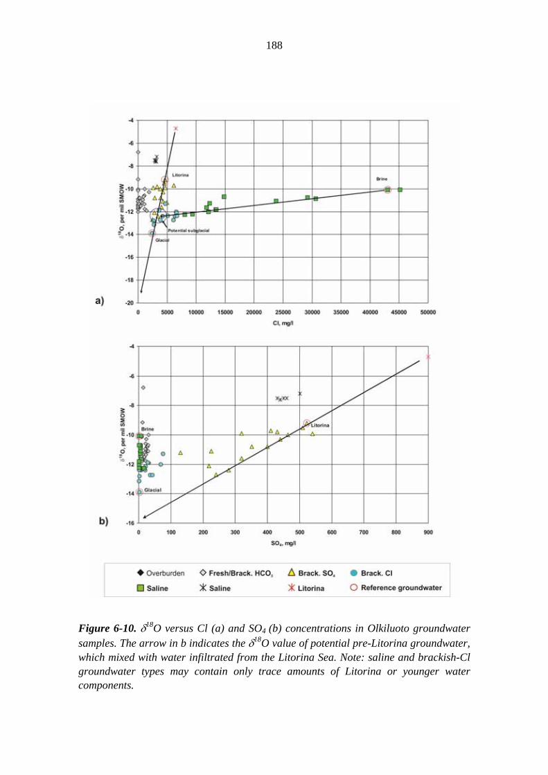
188

Figure 6-10. δ18O versus Cl (a) and SO4 (b) concentrations in Olkiluoto groundwater samples. The arrow in b indicates the δ18O value of potential pre-Litorina groundwater, which mixed with water infiltrated from the Litorina Sea. Note: saline and brackish-Cl groundwater types may contain only trace amounts of Litorina or younger water components.

189

Pre-Litorina groundwater was a mixture of infiltrated dilute glacial meltwater and initial groundwater beneath the ice sheet (termed subglacial water) that had to be more saline and heavier in stable isotopes than the pre-Litorina initial groundwater mixed in Litorina reference groundwaters. This is supported by glacial reference groundwaters, which show higher Cl and δ18O contents than the estimated pre-Litorina initial groundwater above. The estimation of the Cl content in the subglacial groundwater requires an approximation for δ18O in glacial recharge (Cl was 0 mg/l for calculation purposes) and δ18O in subglacial groundwaters. The review of glacial waters by Pitkänen et al. (1999) suggested δ18O values between -22‰ to-20‰ for glacial meltwater as well as the mixing line from the Litorina estimate, via Litorina and glacial reference groundwaters in Figure 6-10a.

The dilution trend of saline groundwaters, which seems to have a lower gradient in brackish-Cl groundwaters, indicates mixing of several water types, whereas the presented straight part of this dilution trend suggests two end-member mixing. The samples forming the straight line represent the deeper part of the Olkiluoto bedrock below 400 m depth. The line may represent long-term dilution that ends up with potential subglacial groundwater. The δ18O value in subglacial initial groundwater would be about -12‰ or slightly less and, assuming a δ18O value of infiltrated meltwater of -22 to -20‰, roughly half the pre-Litorina groundwater would have been water derived from the Weichselian ice sheet. Hence the Cl concentration of subglacial groundwater in the upper part of the bedrock would have been about 3500 mg/l before meltwater intrusion, as is also suggested in Figure 6-10a. The estimate for δ18O in subglacial initial groundwater has decreased from that presented in previous reports by Pitkänen et al. (1999, 2004), as a result of the review of stable isotopic data of groundwaters (Hellä et al. 2005).

The initial waters that were used in mass-balance calculations for interpreting the evolution of the groundwater at Olkiluoto since deglaciation are shown in Figure 6-9. This figure also describes schematically the changes in the hydrogeological conditions at the site throughout its post-glacial history, with salinity estimates of the different initial waters. The upper part shows salinity changes in recharging waters linked to the Baltic stages at Olkiluoto, where the recharge from the freshwater Ancylus Lake has been presumed to be negligible. The left hand side shows the predominant concentration gradient of groundwaters since glacial meltwater infiltration. The salinity of saline reference water has been used as an initial water in mass-balance calculations, because samples with higher salinity do not seem to show any post-glacial indications (Pitkänen et al. 1999, 2004). The salinity gradient at the beginning of the Litorina stage is considered to follow the current salinity trend of brackish-Cl and saline groundwaters below 200 m depth (Figure 6-5), because these groundwater types contain only minor indications, at most, of younger groundwater components. The gradient at shallower depths is difficult to estimate, due to younger groundwaters dominating this depth interval. Presumably the salinity of estimated pre-Litorina initial water has been dominant at depth, where brackish-SO4 type groundwaters prevail at present.

190

Each calculated groundwater sample has been concatenated to the initial waters in a unambiguous manner, which makes it possible to solve the results of chemical mixing using these initial waters (see Chapter 6.5.1). The figure shows schematically the concatenations to current groundwater types. The splitting of the data into complex flow paths used in mass-balance models has been discussed in detail by Pitkänen et al. (1999, 2004) and Luukkonen et al. (2005). The minor mixing paths of meteoric and Litorina waters to deeper groundwater types presented in Figure 6-9 may also result from contamination along short-circuits formed by boreholes.

The steady-state assumption should be obeyed in chemical reactions described in mass-balance models along flow paths. For example, meteoric water reaches calcite saturation soon after infiltration at Olkiluoto. If a flow path calculated by the mass-balance method were too long, calcite dissolution and possible precipitation beyond its saturation point could compensate each other, resulting in no carbonate reactions. Therefore, single models have been limited to short, complex paths (see Pitkänen et el 1999, 2004) in order to gain an understanding of water-rock interactions and pH and redox sensitive processes.

6.3.2 Hydrogeological information

6.3.2.1 Post-glacial land uplift and sea level rise The land is rising in relation to sea level by several millimetres per year in Finland (Eronen et al., 1995). Changes in the shore level are due to the combined effect of two vertical movements, glacio-isostatic land uplift and glacio-eustatic sea level rise (Påsse, 1996). Northern Europe was covered by a huge ice sheet during the last ice age, the load of the thick ice sheet depressed the earth's crust by several hundreds of metres and the release of this load as the ice sheet melted resulted in a strong rebound. In early post-glacial time, land uplift was much more rapid than at present, and the rate of uplift has decreased gradually over the past few thousands of years.

The melting of the ice sheets significantly raised the global sea level until 6000 BP. Whilst the glacio-eustatic sea level rise has clearly been lower than the glacio-isostatic uplift (Figure 6-11), it has, however, reduced the impact of uplift. In addition to the effects of eustasy, the shore level changes in the Olkiluoto area were also influenced by the water level changes during the period of the Ancylus Lake.

Whilst the present (about 6 mm per year in the Olkiluoto area) and future shore level changes are significantly lower than in the past, the land is still expected to rise relative to sea level by several tens of metres in the Olkiluoto area over the next 10 000 years.

The gradient of the groundwater table is the primary driving force for groundwater flow in the bedrock. The hydraulic gradient makes the fresh, near-surface water flow deeper into the groundwater system, mixing it with water of different types and of different salinities. The net effect of the post-glacial uplift and the global sea level rise enlarges the area of Olkiluoto Island and raises the groundwater table. The uplift of the groundwater table increases the flow of fresh water deeper into the bedrock, and

191

eventually, after perhaps two thousand years, the saline water in the upper part of the bedrock will be flushed by fresh water. The transient process started from the moment when the highest hills at Olkiluoto rose above sea level about 3000-2500 years BP, and since then the hydrological conditions at Olkiluoto have been subject to continual changes, which have to be considered when analysing the groundwater flow. Påsse (1996) has constructed a mathematical model for both the land uplift and the sea level rise in the area covered by the Scandinavian ice during the Weichselian glaciation. The change in shore level is obtained as the sum of the effects of uplift and eustasy (Figure 6-11). According to the model the land will rise relatively to sea level by about 40 metres during the next 10 000 years. Eronen et al. (1995) have studied the shore level changes of the Baltic Sea and the land uplift process in south-western Finland during the last 8000 years and the empirical data obtained by studies on sediments in small lakes (Figure 6-11) is consistent with the model by Påsse (1996).

Figure 6-11. The shore level displacement in the Olkiluoto area since 20 000 BP (calendar years) until 10 000 AB. Negative axis represents the past and positive the future, with zero denoting today. Circles represent the empirical data from sediments in small lakes from Eronen et al. (1995).

192

6.3.2.2 Hydraulic properties of bedrock and groundwater

Transmissivity of deformation zones

The transmissivities presented here are based mainly on flow logging in boreholes (Pöllänen & Rouhiainen 1996a,b, 2000, 2001, 2002a,c,d,e, Rouhiainen 2000), although in some cases double-packer (HTU) results (Hämäläinen 1991a,b, Kuusela-Lahtinen & Front 1991a,b,c, Hämäläinen 1997a,b,c,d,e, Hämäläinen 1998, Hämäläinen 2003a,b,c, Hämäläinen 2004) and single-hole long-term pumping results (Ylinen 1993, Niva 1996, Jääskeläinen 1998) have also been used. For borehole sections where two or three methods have been used, the determination of the most representative value has been based on expert judgement and the conclusions are reported in Ahokas (2001, 2003). All measured transmissivities are presented in Figure 6-12. The transmissivities of structures in the flow model are based either on measured single values or, if several values are available, on the geometric mean, i.e. the same structure intersects several boreholes. When the measured transmissivity is lower than the corresponding hydraulic conductivity of the bedrock (see next section) it is proposed that the values presented in Table 6-4 should be used. These values have been determined by taking into account the depth dependency found from the determination of the hydraulic conductivity of the bedrock and using it to develop a stepwise-decreasing transmissivity for the R-structures in question. The transmissivity of R-structures without measured values is estimated to be in the order of –5 (log T). Hydraulic conductivity of the bedrock The effective hydraulic conductivity, Keff, of the rock mass between explicitly modelled structures is calculated based on the geometric means of measured high transmissivities, TG, and their frequency — or more precisely the distances between high transmissivity values, dist, outside the structures, according to the equation:

dist/Geff TK = Transmissivities higher than –8 (log T) are taken into account and values in close proximity are estimated as belonging to a single hydraulic feature (narrow zone). Measured transmissivities are presented in Figure 6-13 as cumulative plots and divided into five depth intervals, i.e. 0–50, 50–100, 100–200, 200–400, 400–900 m below sea level. The corresponding distances between transmissive features are presented in Figure 6-14.

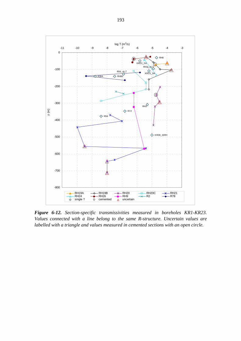
193

KR23_2HRH11_ALT

KR23_3HR56_ALT

RH80R10A

RH3

R72

R56

KR08_13RH

RH8

-800

-700

-600

-500

-400

-300

-200

-100

0-11 -10 -9 -8 -7 -6 -5 -4 -3

log T (m2/s)z

(m)

RH19A RH19B RH20 RH20C RH21RH24 RH26 RH9 R2 R78single T cemented uncertain

Figure 6-12. Section-specific transmissivities measured in boreholes KR1-KR23. Values connected with a line belong to the same R-structure. Uncertain values are labelled with a triangle and values measured in cemented sections with an open circle.

194

Table 6-4. The transmissivity of deformation zones which intersect boreholes. The transmissivities of structures with a low measured value have been modified to be higher than the corresponding value in the bedrock and are also assumed to be depth-dependent.

R-structure

Single-T or geometric mean

(log m2/s)

log T (depth 0-50 m)

log T (Depth 50-100 m)

log T (depth 100-200 m)

KR08_13RH -5.0 KR23_2H -5.8 KR23_3H -5.2 R10A -8.8 -7 -8 -8.5 R2 -7.2 -7 R56 -8.4 -7 -8 R56_ALT -6.9 R72 -6.8 R78 -7.3 -7 RH11_ALT -4.9 RH19A -4.4 RH19B -4.8 RH20 -4.7 RH20C -6.4 RH21 -7.6 -7 RH24 -5.1 RH26 -5.9 RH3 -5.3 RH80 -7.5 -7 RH9 -6.0 RH8 -4.7

Calculated effective hydraulic conductivities for different depth intervals are presented in Figure 6-15. The rounded values, which it is proposed to use in the flow model, as well as the curve for Keff used in the earlier modelling case (Löfman 1999), are also shown. The values of Keff which it is proposed to use in the flow model are also presented in Table 6-5 below.

195

0

10

20

30

40

50

60

70

80

90

100

-9 -8 -7 -6 -5 -4log T

cum

ulat

ive

%

T-(0-50 m)T-(50-100 m)T-(100-200 m)T-(200-400 m)T-(400-900 m)

Figure 6-13. Cumulative plots of transmissivities measured in the bedrock (outside R-structures) and divided into five depth intervals.

0

10

20

30

40

50

60

70

80

90

100

0 1 2 3log (distance, m)

cum

ulat

ive

%

dist-(0-50m)dist-(50-100m)dist-(100-200m)dist-(200-400m)dist-(400-900m)

Figure 6-14. Distances (log) between transmissive features in the bedrock outside explicitly modelled structures as cumulative plots and divided into five depth intervals.

196

0

100

200

300

400

500

600

700

800

900

1000

-12 -11 -10 -9 -8 -7 -6log (K, m/s)

dept

h, m

Figure 6-15. Effective hydraulic conductivities for different depth intervals (open circle) and the curve for Keff used in the earlier modelling case (Löfman 1999).

197

Table 6-5. Values proposed to be used in the flow model for the bedrock outside explicitly modelled deformation zones.

Depth interval (m) Keff (m/s)

0–50 10–7

50–100 10–8

100–200 3 10–9

200–400 10–9

400– 3 10–10

Its well known fact that the determination of Keff in heterogeneous bedrock is difficult, and the values presented in Table 6-5 and Figure 6-15, therefore, include high levels of uncertainty. The method used for the estimation of Keff above is based on the simplified assumption that transmissive fractures are planar and continuous throughout the bedrock between the deterministic fracture zones, that the distribution of transmissivity for each feature (fracture) follows the distribution shown in Figure 6-13 and that the use of the geometric mean is applicable. Where transmissive features exist, for example, in three approximately orthogonal directions (i.e. one subhorizontal and two vertical, thereby defining a cubic system), the distances between such features in the bedrock are greater than the mean distances found in boreholes and shown in Figure 6-14. This means that values of Keff presented in Table 6-5 are somewhat too high in the subhorizontal direction but somewhat too low in the vertical direction. It is also possible that the highest transmissivities are associated with a few single fractures or narrow fracture zones, and in these cases the values shown in Table 6-5 are too low. For example, if high transmissivities measured in the depth range of 100-200 m are associated with one or two features (one subhorizontal, one vertical) the value of Keff would be in the order of 1 10–8 m/s, because TG is approx. 1 10–6 m2/s and the thickness for the calculation of Keff is naturally 100 m. In this case Keff is approx. three times higher than the value presented in Table 6-5. Generally, the discussion above demonstrates that the values presented in Table 6-5 are not very sensitive to the different assumptions made, in cases where transmissive features are estimated to be continuous and to follow measured T-values - an interpretation which is based on the assumption of radial flow along a homogenous plate. A similar assumption has been the basis for the evaluation of Keff above. The hydraulic conductivity of the bedrock outside the modelled zones depends on the number and density of explicitly modelled zones in the flow model. This effect can be best seen outside the central investigation area, where the number of structures is clearly smaller. It is possible that such “blind” areas may also exist in the central investigation area, perhaps on a smaller scale, e.g. west of borehole KR11, where power lines have

198

hindered investigations. It is proposed that the effect of a lack of explicit deformation zones can be taken into account in the flow model by increasing the value of Keff outside the central investigation area by a factor of 3 to 5. Typically such (modelled) zones exist every 200-300 m in the bedrock and measured transmissivities lie in the range 1E-4 - 1E-5 m2/s. The transmissivity due purely to these zones is thus in the order of 3E-4...5E-4 m2/s or 3E-5...5E-5 m2/s, which makes the total bedrock approximately 3 to 5 times more conductive than the uppermost bedrock for the central investigation area, as shown in Table 6-5. Other properties Values used for the other properties are presented in Table 6-6. The density of the fresh water and the dependence coefficient on chloride concentration are based on the correlation of the measured density and salinity. In order to decrease the spreading of solutes caused by the dispersion, the longitudinal dispersion length was selected to be as small as possible, also taking into account the numerical problems associated with too large a Peclet number when solving the transport equation. The transverse dispersion length was taken to be 25% of the longitudinal dispersion length. The effect of these dispersion lengths is mainly restricted to determining the width of the interface between the fresh and saline water. The value for the diffusion porosity used with the DP model is based on reports (Paulamäki and Paananen, 1995; Paananen and Paulamäki, 1995), in which the diffusion porosities for the migmatitic mica gneiss and pegmatitic granite have been predicted for borehole KR10 and the extended part of borehole KR2. The viscosity of water and the molecular diffusion coefficient of salt in water are well known parameters (Lide 1990). Fracture aperture and spacing were selected in such a way that flow porosity was in line with the values reported in the literature for the crystalline rock.

199

Table 6-6. Hydraulic properties of the bedrock and the groundwater. Initial values (before calibration).

Fresh water density 998.6 kg/m3

Viscosity of water 1.0·10-3 kg/m/s Longitudinal dispersion length 50 m Transversal dispersion length 12.5 m Fracture aperture 1.0·10-4 m Flow porosity in fracture zones (fracture spacing 0.1 m)

1.0·10-3

Flow porosity in sparsely fractured rock(fracture spacing 1.0 m)

1.0·10-4

Diffusion porosity 2.0·10-3 Molecular diffusion in water 1.0·10-9 m2/s

6.3.2.3 Initial and boundary conditions The simulations are carried for a period starting at the early Litorina Stage (about 8000 years BP) and continuing until the present day. The initial and boundary conditions are based on the latest geochemical modelling of groundwater evolution at Olkiluoto (Pitkänen et al. 1999, 2004). The highest hills on Olkiluoto Island rose above sea level about 3000-2500 years BP, resulting in the recharge of fresh water into the bedrock. The net effect of the land uplift and global sea level rise was to gradually enlarge the area of the island and increase the elevation of the groundwater table. The specified pressure representing the current elevation of the groundwater table is used as a boundary condition for the area of the surface, which at each time step is above the sea level, with zero pressure on the remaining area. Thus, zero pressure is applied on the whole top surface as long as the island is below sea level. The groundwater level at Olkiluoto is clearly below the surface and there is no clear correlation between it and the surface topography (Löfman 1999). Therefore, the land uplift scenario of Påsse (1996) is not synonymous with the uplift of the groundwater table. For example, at present the highest point at Olkiluoto is 18 m OD, whilst the corresponding elevation of the water table is only 10 metres. In addition, water table data available for the Olkiluoto area (Ahokas 1993, Hänninen 1996) are incomplete (e.g. they do not cover the mainland and the neighbouring islands). In this study, a relatively simple linear transformation (Löfman 1999) of the topography (Autio 1991) (water table = 0.56 x topography) was used for the area where the water table data were unavailable. The same transformation is applied to obtain the net uplift of the groundwater table from the net land uplift.

200

In the remainder of the modelled volume, the initial pressure was assumed to be hydrostatic and was defined on the basis of the initial salinity concentration. On the vertical boundaries hydrostatic initial pressures were employed for the whole simulation period, whilst at the base of the model at a depth of 2000 m, a no-flow boundary condition was applied. According to interpretations, the hydrochemical conditions during the Litorina Sea stage were different from those of today. For a considerable period during this period the TDS concentration of sea water was much higher (about 11 g/l, calculated as NaCl) than today (5.6 g/l). The groundwater in the upper part of the bedrock was a mixture of subglacial groundwater, diluted by glacial meltwater during the deglaciation period, (note that in Chapter 6.3.1 and in Figure 6-8 TDS Cl concentrations are used instead, as they are useful in chemical interpretations). Pitkänen et al. (1999) estimates the maximum TDS of the mixture above the current SO4-poor brackish and saline groundwaters to have been about 2.5-3.3 g/l, which would have enabled seawater infiltration into the bedrock through the seabed sediments. Deeper in the bedrock salinity increases and groundwater is composed of brackish and saline water layers. Thus, the initial salinity concentration in this work was originally assumed to increase from 3.0 to 4.1 g/l to a depth of about 200 m and follow the present measured values to a depth of about 800 m (Figure 6-16). A constant salinity, corresponding to the highest measured value (83 g/l), was employed at the base of the model (2000 m depth). Seawater recharge is assumed to have occurred from the beginning of the simulation, with the concentration of seawater decreasing from higher Litorina stage value to its present value (Figures 6-9 and 6-17).

201

Figure 6-16. Measured TDS concentrations as a function of depth and the salinity model employed as an initial conditions for concentration. Initial model (before calibration).

Figure 6-17. Salinity of the Baltic seawater employed as a boundary condition for concentration on the top of the model. Initial model (before calibration).

202

6.4 Interaction with other disciplines Hydrogeological and hydrogeochemical interpretations and modelling efforts significantly depend on the concept of site geology. Both disciplines make use of the prevailing hydrostuctural model, that is based on the geological deformation zone model. Groundwater flow is simulated in a straightforward manner in the hydrostuctural model, whereas geochemical mass-balance modelling tries to use hydraulic connections in interpreting and composing flow paths which concatenate single samples with initial groundwaters (Figure 6-9), though chemical and isotopic compositions with the apparent ages of samples impose major boundaries in this task (Pitkänen et al. 1999, 2004). Additional information has been gained on flow paths from mineralogical and chemical variations in the bedrock (from the lithological model) or fractures, which may be reflected in the groundwater compositions at the site, particularly regarding trace element or isotopic compositions. The interpretation and modelling of hydrogeochemical evolution also uses information on overburden geology, mineral compositions, the chemical composition of minerals, the results of chemical and isotopic compositions and, in particular, fracture mineralogy, such as that presented by Blyth et al. (2000) and Gehör et al. (2002).

Chapter 6.3 presented a discussion on the interaction of hydrogeology and hydrogeochemistry at the initial stage of model development. The available qualified hydrogeochemical and hydrogeological data are integrated together for the Olkiluoto site area (see Figure 6-16). The data used for this integration were collected during the baseline characterisation, and the inevitable tool for this integration is the prevailing view of the structural model, together with estimations of the hydraulic properties of the deformation zones. The baseline integration follows a "history-to-present" oriented approach that attempts to simulate compositional changes in the groundwater as a function of time within the bedrock. In this way hydrogeochemical modelling will produce a knowledge of the past for the hydrogeological modelling. This knowledge of the past TDS distribution is needed to determine the initial state for the time-dependent modelling. Hydrogeological simulations are required to extrapolate the evolution of the groundwater composition from the past, via the present to extrapolations into the future.

The observations of present day conditions are needed for model calibration, which takes place at groundwater sampling locations, i.e. in boreholes. The groundwater compositional distributions, i.e. initial water compositions, are also superimposed on the prevailing hydrostructural model. During the analysis of the modelling results, a comparison of these 3-D distributions with the flow simulations may give important information on the differences in relative flow dynamics of different R-structures, and therefore provide feedback to the hydrogeological model and ultimately to the Site Model (Figure 6-18). The numerical pressure simulations may also give direct feedback on the competence of the Site Model, with reference to how well the model can response to measured pressures in the boreholes.

203

Figure 6-18. Iterative integration concept during baseline conditions and the ONKALO phase. A gradual development of hydrogeological and hydrogeochemical models is expected as integration progresses and the Site Model develops.

204

6.5 Modelling results

6.5.1 Hydrogeochemistry Mass-balance calculations

Mass-balance mixing–reaction models are used to determine the magnitude of interpreted evolutionary processes, based on data from hydrochemistry, isotopes, mineralogy and solubility calculations. The modelling tests the interpretation of the hydrogeochemical evolution by providing information on plausible reactions and their extent, on the level of mixing in the system and on any uncertainties in the concept and the data. Successful modelling may also increase confidence in the ability to predict hydrogeochemical conditions in the geosphere following repository closure, to identify potential environmental changes in the future and to set initial and boundary conditions for evolutionary predictions used in the Safety Case. The modelling tests the reaction and mixing hypotheses by constructing mass-balance models, which describe the changes in chemical and isotopic composition between initial water and down-gradient water samples. The model developed for mass-balance calculations between any points along a chosen flow path is of the form:

Initial water(s) + "Reactant phases" → Final water + "Product phases" where reactant phases enter the initial water or initial mixture and products leave to produce the composition of the final water. The results presented in this chapter are extensions to the previously calculated mass-balance models of Pitkänen et al. (1999, 2004) and they increase the data on the initial water mixing proportions used in the characterisation of 3-D hydrogeochemical conditions at Olkiluoto (Luukkonen et al. 2003). The previous models were computed with the NETPATH (Plummer et al. 1994) program, whereas PHREEQC (Parkhurst & Appelo 1999) is used for the subsequent models (Luukkonen et al. 2005). Mass-balance models define the mixing proportions of initial waters and the net geochemical reactions of minerals and gases that may account for the observed composition of the final water. The results of conservative mixing are important for the task of integration, and all calculated models (on 93 groundwater samples) are used in this chapter. The mass transfer due to water-rock reactions and their distribution in different parts of the bedrock, as described by Pitkänen et al. (2004), is summarised in Chapter 6.2.2. The results of the most recent calculations (on 33 samples) are not reported yet. They will be reported separately (Luukkonen et al. 2005). Although the calculated mass transfer due to water-rock reactions does not have a straightforward effect on the mixing proportions, these reactions form important boundary conditions in evaluating the plausibility of the calculated mass-balance model. Therefore, they also have an indirect effect on the results of mixing. The inclusion of isotopic data in reaction modelling provides additional criteria for testing a reaction and

205

mixing hypothesis (Plummer et al. 1994). Carbon and sulphur isotopic data were used in previous NETPATH calculations to provide further insight into the pH and redox reactions of minerals and gases, which are controlled by carbon and sulphur cycles with isotopic fractionation (not included in PHREEQC version 2). In recent calculations stable isotopes of water (2H and 18O) are used in addition to Cl to provide additional conservative constraints on mixing. PHREEQC can calculate mass transfers within specified compositional uncertainty limits, which makes it possible to test the fitting of several conservative traces simultaneously in models (which is not possible with NETPATH). The initial stage for the calculations is the Weichselian deglaciation at the site (as described in Chapter 6.3.1) and the groundwater column is divided into two initial waters: deep, saline groundwater, which is not observed to be chemically disturbed by later groundwaters, and brackish groundwater (subglacial), which is interpreted to be evolved before deglaciation, and represents the average composition of brackish groundwater in the upper part of the bedrock. The other initial water types mixed in the groundwater system are glacial meltwater, Litorina and current Baltic seawaters, and modern meteoric recharge. The mixing of these initial waters with plausible hydrogeochemical interactions is able to explain all the observed compositional varieties which have evolved since the Weichselian glaciation at Olkiluoto. In most cases two to three initial waters comprise over 90% of any single groundwater sample. Proportions which are less than 10% can be considered unreliable, due to interpretational uncertainties in the initial waters. The calculated distribution of different initial waters is presented with depth in Figure 6-19. Currently infiltrating water types, i.e. meteoric and Baltic seawater (which has only a minor role) are generally limited to the upper 150 m of the bedrock, but with a few exceptions, such as at a depth of 250 m in borehole KR7, which intersects structure R20B. However, other samples taken from the same zone from different depths do not show abnormal meteoric input. The two observations of meteoric groundwater between 300 - 400 m depth (both from borehole KR20) probably represent partial storage of water which has flowed downward in the open borehole (Hellä et al. 2005). Litorina seawater is a significant component between 100 and 300 m depth, and pre-glacial groundwater initial water types (saline and subglacial) are totally dominant at greater depths. Near the shoreline the proportion of Litorina seawater increases at shallower depths (Pitkänen et al. 1999, 2004), indicating that meteoric water may be absent beneath the sea (confined discharge near the shoreline is likely to be taking place) and the whole hydrochemical column may be 100 m higher than onshore. The maximum proportion of glacial water is found approximately from 100 m to 200 m depth, and the proportion of glacial water decreases steadily with depth, such that its proportion is less than 20% in the saline groundwater zone (below 400 m depth). The Weichselian glaciation is not necessary the only source of glacial water, particularly in

206

the deep saline groundwater system, where the glacial component may contain water from other older, cold periods, as is suggested by the Cl -18O diagram (Figure 6-10a).

Figure 6-19. Depth distributions of mixing fractions of interpreted initial waters in Olkiluoto groundwater samples. Trend lines show depth distributions of the initial (groundwater types) in the Olkiluoto area. Visualisation The 3-D visualisations of initial water distributions are built up from three separate processes. In the first process the geochemical samples are characterised and considered from the viewpoint of three different recharge/discharge areas on Olkiluoto Island. These geochemical environments are topographic highs, coastal areas and the Korvensuo area. In the second process, the characteristics defined for the three areas are expanded in the studied Olkiluoto volume. In the final process, the extrapolated geochemical distributions are superimposed on an Olkiluoto fracture zone model. The

207

final results of this three-stage process are presented as colour gradient images superimposed on the fracture zones considered. The modelling approach contains the following built-in assumptions. It assumes that the analysed and interpreted geochemical results do not represent their sampling locations only, but are indicative of broader characteristics that can be extrapolated into larger volumes of the bedrock. Furthermore, the superimposition of distributions on a fracture zone model makes the assumption that practically all the geochemical results used in the visualisation approach have been sampled from fracture zones. The visualisation method is outlined below and examples of the results of this modelling are presented in the final part of this Chapter. Currently, the method illustrates the general baseline conditions. However, the approach is designed so that the geochemical anomalies caused by the construction of the ONKALO or the addition of more detailed baseline features, can be mapped and included in the visualisations. The local model modifications can be made as soon as an interpreter is able to summarise the strength and extent of the local anomalies. Geochemical characterisation – first process

Figure 6-19 illustrates the definition of the three different geochemical areas. The division is made only to non-saline ([Cl-] < 8 g/l) samples above -400 m depth (Fig 6-20). The saline ([Cl-] > 8 g/l) data from depth is common to all three geochemical areas, as the depth distributions of saline waters in different parts of the site seem to be similar. Furthermore, the number of saline samples is insufficient to allow a reliable investigation of the differences between the areas. The topographic highs, defined with 19 groundwater samples, are located in the central part of Olkiluoto Island where the watershed lies, and are characterised by a pronounced recharge of meteoric water. The two coastal areas, consisting of 32 samples (Figure 6-20), represent low lying recharge/discharge environment on the N and S coasts. The Korvensuo area consists of 26 groundwater samples located close to the Korvensuo reservoir.

208

Figure 6-20. The three different geochemical environments of the Olkiluoto sampling area. The colour bar refers to the groundwater table in metres above sea level (POSIVA 2003-02).

The geochemical characteristics of the three Olkiluoto surficial groundwater flow areas (Fig. 6-20) are concentrated into three primary "data" centroids (Fig. 6-21). Each centroid extracts the geochemical depth characterisitics for the flow area in question (cf. Fig. 6-22). The mode characteristics (centroids) are assigned on the Olkiluoto map on the topographical and locational grounds. The judged aerial set-up of primary centroids is shown in Figure 6-21. The centroid locations designate either high topography or artificial lake (recharge) or low topography coastal (discharge) areas of the Island. The eight centroids, plotted in Fig. 6-21, divide the Olkiluoto well characterised areas into seven sectors. It becomes evident that these sectors are necessary for 3-D expansions of geochemical characterics.

209

Figure 6-21. Location of primary centroids for Olkiluoto Island, marked with white diamonds. The WCA (Well Characterised Area) is indicated with a grey box. The sampling locations of the different geochemical areas are illustrated as in Figure 6-19. The colour bar refers to the groundwater table in metres above sea level (from POSIVA 2003-02).

Considering each characteristic area, the initial water distributions (as a function of depth) are presented with smoothed and fitted lines (Figure 6-22a, d, and h). These fitted distributions must sum up to unity, as presented in Figure 6-22b, e, and i. As an additional validity measure, the calculated Cl distributions have been considered against the measured Cl values. The results of these considerations are shown in Figure 6.22c, f and j. The equation for determining the Cl distribution is presented in Luukkonen et al. (2003). Note that the heights and widths of individual initial water distributions affect the form of the calculated Cl distribution. In other words, if a calculated Cl distribution does not fit the measured Cl values, changes must be made to the inferred initial water distributions.

210

Figure 6-22. Geochemical distributions for the centroids of topographic highs (a,b,c), coastal areas (d,e,f) and the Korvensuo area (h,i,j). The lines/areas indicate calculated distributions and dots measured values (Colour indexes for different water types: green=current, red= Litorina, blue=glacial, cyan=subglacial and grey/black=Saline; In diagrams c, f and j black line=calculated [Cl] and grey dots = measured Cl values.

211

The clearest deviations between the primary centroids among the three geochemical environments can be seen in the behaviour of the current water (current water is the sum of meteoric and Baltic Sea water). In the centroids of the topographic highs (Fig 6-22a-b) and the Korvensuo area (Fig 6-22d-e), current water dominates down to -100 m and diminishes towards depths of -200…-250 m. In the coastal areas, the current water domination extends only to the first -50…-70 m, and below 150 m depth the proportion of current water practically vanishes. Litorina water is the dominant water between -100 and -250 m in all geochemical environments. In coastal areas the maximum Litorina proportions are reached at slightly shallower depths than elsewhere. The Litorina maximum has sunk to -200…-220 m in the centroid of the Korvensuo area (Fig 6-22). In addition, the Litorina maximum is smaller and covers a slightly narrower depth range than elsewhere. Saline water (Figure 6-22), indicated by black lines (a, d, and h) and grey areas (b, e, and i), is described in all primary centroids by using 16 saline samples, i.e. below -430 m the depth distributions are similar in all primary centroids. Note that the Cl concentration is limited to 22 g/l (Pitkänen et al. 1999) in this approach, though the measured concentrations tend to be considerably higher at depths below 700 m (The maximum measured value is 53.1 g/l from borehole KR2). Expansion of distributions – second process Regression calculations are used in the expansion of the three geochemical mode characteristics. The three distributions (Figure 6-22) are used to define seven sectors that cover the onshore area of Olkiluoto Island, so that each sector-defined volume can be managed with the three bounding centroids (Figure 6-23a). The spatial expansion of the primary centroids begins with the creation of an array of secondary centroids, and then continues with extrapolation calculations of water fractions into each secondary centroid. Figures 6-23b and c illustrate an example of linear regression calculations. The depth vs. initial water distributions defined for a secondary centroid (14, 3) – see Figure 6-23a – are regression results from the distributions of the primary centroids 1, 2, and 8 (cf. Figure 6-21). By applying similar extrapolations to all secondary centroids, the complete volume of the WCA can be characterised. The array of secondary centroids is a redefinition of the Olkiluoto baseline. The array provides the possibility of adding local heterogeneities to the general baseline visualisation that was created with just three geochemical mode characteristics and eight primary centroids. Local heterogeneities can be, for example, the Baltic Sea areas, on the northern and south-western edges of the WCA (cf. Figure 6-21), or local compositional heterogeneities within the WCA volume (identified from the baseline samples).

212

The baseline conditions are gradually lost as the excavations proceed. The local anomalies created by the ONKALO construction will, step by step, modify the secondary centroid array. The arrays with time steps will be saved, and gradually the 3D mapping/visualisation of groundwater geochemistry begins to describe the transient groundwater evolution of open tunnel conditions. Superimposition on fractures – final process The superimposition of a centroid array onto a fracture zone model demands a special treatment for the zones. As Figure 6-23b indicates, each secondary centroid contains variables with strong gradient variations (e.g. current or Litorina water distributions). Furthermore, gradient variations will be even more frequent when visualising the disturbances caused by the construction of the ONKALO. The successful visualisation of these gradients requires a smooth rendering method for colour gradients within the fracture zones. This task is carried out by generating a gradient change sensitive rendering network into the fracture zones. The network needs to be adaptive, i.e. the network must become denser at locations where the changes in gradients occur. The adaptability is expected to be especially important while visualising the effects of ONKALO construction. An example of an adaptive network created for the current water distribution in the WCA volume for the baseline conditions is presented in Figure 6-23d.

213

Figure 6-23. a) Extrapolation method for initial water distributions from the primary centroids (red dots) to an array of secondary centroids (blue dots). b) Distributions of current (green), Litorina (red), glacial (blue) and saline (black) waters in the secondary centroid (14,3). c) Cumulative presentation of water fractions. Subglacial water is presented with light blue. d) Adaptive network generated in the structural model for distributing the current water.

a) b)

c) d)

214

The modelled baseline water distributions within the WCA volume are presented in Figure 6-24, in which the viewpoint and axial dimensions for the illustrations are the same as in Figure 6-23d. The modelled volume extends only to a depth of -900 m, because there are no quality evaluated geochemical data available below this depth. Otherwise, the fracture zone geometry adapted to the illustrations is the same as used in the hydrogeological calculations (Chapter 6.5.2). Current water is the dominant water in most parts of the WCA volume at depths above -150 m. According to Figure 6-24, the thickness of the current water layer becomes thinner at the northern edge of the WCA. However, this is probably an artefact that originates from extrapolating the coastal type centroid characteristics (primary centroids 2 and 3, Figure 6-23a) towards the north. Figure 6-21 indicates that the Baltic Sea shore is met before the northern edge of WCA. The actual depth distribution of current water below the areas of sea is likely to deviate from the present estimates, that are based on the sampling carried out on Olkiluoto Island. Furthermore, when considering future attempts at visualisation, it will be necessary to handle separately the meteoric and Baltic Sea water fractions, instead of combining them, as is currently the case. The Litorina water distribution within the WCA (Figure 6-24) shows that the smallest amounts of Litorina water are stored in the eastern boundary of the WCA. The interpretation is opposite to what might be expected, when considering the amount of Litorina water on the northern edge of the WCA. By comparing these results with those of Figure 6-21, it seems that these interpretations are in contradiction. Both the northern and eastern edges of the WCA have low elevations or are beneath the sea and it would seem more likely for these areas to be characterised by Litorina water distributions that are appropriate to depths below the Baltic Sea. The concentrations of glacial water below Olkiluoto Island are generally relatively small, and this feature is replicated well in the results of the modelling. In all three characteristic areas (Figure 6-22) the glacial fractions comprise relatively mode-less distributions that extend to considerable depths. The result possibly indicates that the Pleistocene hydrostatic pressure, originating from the overlying ice sheet, was able to push glacial meltwater to great depths. However, meltwaters did not displace extensive subglacial or saline waters from the bedrock fracture network. The Saline water distribution behaves monotonously in the WCA volume. This is due to the simple fact that the saline water distributions are similar in all three characteristic areas (Figure 6-22). However, this simplification receives its justification from the geochemical data and aerial geochemical variations at great depths are hard to prove from the sampled material. Subglacial water is stored mostly at depths -300...-400 m, where the concentrations of subglacial water are relatively high. Typically, the maximum fractions vary around 0.6–

215

0.7, with the subglacial water layer being located above the saline water. The subglacial layer behaves almost as uniformly as the saline water layer. The final diagram in Figure 6-24 is a simple error indication diagram. It does not measure reliability of the calculations for the illustrated initial water fractions, but simply the level of success of the extrapolations. Since each initial water distribution is extrapolated separately into the WCA volume, it is possible for water fractions not to sum up to unity everywhere in the model volume. The error diagram in Figure 6-24, however, indicates that this condition is undetectable, at least at the current scale of visualisation.

216

Figure 6-24. Modelled initial water distributions within the fracture zones of the WCA. The illustrated structural blocks are viewed from the SW. The length of North and East arrows is 300 metres. The ground level boundaries of the WCA are also shown in Figure 6-21. The colour of the error distribution (at lower right) would deviate from green if the sum of the extrapolated initial water fractions deviated from unity. Note that the colour scale for the glacial water fractions ranges from 0 to 0.5, and that the colour scale for the error distribution ranges from -1 to 1.

Current Litorina Glacial

Saline Subglacial Error

217

Figure 6-25 represents the calculated TDS distributions within the fracture zones of the WCA. The calculated TDS is simply the sum of initial water fractions and their modal TDS values within the WCA volume. Note that because the maximum Cl concentration is restricted to 22 g/l in the current model, the maximum TDS concentration is restricted to 35 g/l. The dark red colour in Figure 6-25 should be interpreted as meaning that those areas contain salinities that exceed the limit of 35 g/l, and that they contain potentially very high salinities, as observed in the measurements in boreholes. Figures 6-26 and 6-27 illustrate the water and TDS distributions within the modelled structures (fracture zones) RH19B and RH20AB, which will be the first notable hydrogeological structures to be penetrated by the ONKALO within the next few years. Both structures extend to the saline groundwater layer in their deeper parts, although the salinity in zone RH19B only just exceeds 10 g/l. In 2005 the ONKALO is expected to intersect zone RH19B in the transition zone between the current, primarily meteoric, water and the zone dominated by Litorina initial water. The current water will be the major component and its fraction may be 80%, resulting in a TDS value of about 2 g/l at the expected point of intersection.

218

Figure 6-25. Calculated TDS-distributions within the fracture zones of the WCA. The illustrated structural blocks are viewed from SW. The length of North and East arrow is 300 metres. The deep boreholes from KR1 to KR28, and the pre-ONKALO pilot hole PH1 are sketched in the Figure. Due to restriction in the calculation the TDS maximum concentration is limited to 35 g/l.

g/l

TDS concentration

219

Figure 6-26. Modelled initial water distributions within fracture zone RH19B. The view is perpendicular to the fracture plane, up and from the south. The length of the North and East arrows is 100 metres. The colour scales are as in Figures 6-24 and 6-25. In other words, the scale from deep blue to deep red is in the range [0 - 1] in the current, Litorina, saline, and subglacial illustrations. In the glacial illustration the scale is in the range [0 - 0.5], and in the case of TDS the scale is in the range [0 - 35] g/l.


Saline Subglacial TDS

220

Figure 6-27. Modelled initial water distributions within fracture zone RH20AB. The view is perpendicularly to the fracture plane, up and from the south. The length of North and East arrows is 200 metres. The colour scales are as in Figures 6-24 and 6-25. In other words, the scale from deep blue to deep red is in the range [0 - 1] in the current, Litorina, saline, and subglacial illustrations. In the glacial illustration the scale is in the range [0 - 0.5], and in the case of TDS the scale is in the range [0 - 35] g/l.


Saline Subglacial TDS

221

6.5.2 Hydrogeology

The objective of the hydrogeological modelling is to characterise the evolution of the groundwater flow conditions at Olkiluoto during the post-glacial period, since the early Litorina Stage. The modelling is carried out by means of a finite element simulation of coupled groundwater flow and solute transport from 8000-7000 years BP up to the present day. Details of the modelling approach are presented in the studies by Löfman (1996, 1999, 2000). The simulations were carried out with a finite element program FEFTRA (FEFTRA 2005) developed at VTT Processes for the modelling of groundwater flow, solute transport and heat transfer.

6.5.2.1 Calibration An essential part of the groundwater flow analyses is calibration, which strives to ensure that the flow model corresponds to the hydraulic characteristics of the real system as well as possible. In the calibration, the hydrogeological properties of the flow model are modified until an acceptable agreement with field observations is achieved. Any input parameter of the flow model can be calibrated, i.e. the shape and extent of the fracture zones, the hydraulic properties of bedrock, the boundary conditions, etc. In this study a special emphasis is placed on an integration of hydrogeology and hydrogeochemistry. Hydrogeochemical data are used to improve the flow model, whereas the results of the flow simulations are compared with the corresponding interpretation of the hydrogeochemical conditions. The previous integration effort was carried out as part of the international EQUIP project (Bath et al. 2000, Gehör et al. 2002), in which the agreement between the flow simulations and hydrogeochemistry was not optimal. In the upper 300 m of the bedrock the simulated groundwater was clearly more diluted than that observed in borehole measurements. The EQUIP project did not include any calibration. The calibration in this work is focused on improving the agreement between the simulated results and hydrogeochemistry in the upper part of the bedrock. Thus, the adjusted parameters were chosen to be those that were considered to have the greatest effect on solute transport. The calibration is carried out using a manual trial-and-error technique and the agreement of the flow model with the hydrogeochemistry is evaluated against the measured salinity and pressure in the deep boreholes. The flow model that gives the best agreement with the field data is chosen to be the model to be used for the groundwater flow analysis.

222

The main problem in the calibration was to reach salinity values in the upper part of the solution domain as great as those measured in the field investigations. Consequently, the following actions were taken in the calibration:

• The effect of matrix diffusion was considered by replacing the EC model with the DP model

• Flow porosity was increased by one order of magnitude • Dispersion length was reduced to 30 m • The initial salinity distribution curve was elevated by 100 m (Figure 6-28) • The initial salinity distribution was decreased at a depth of 0-200 m (Figure 6-

28) • The duration of the highest salinity of sea water (11 g/l) was increased on the top

boundary (Figure 6-29) • The highest salinity of sea water was increased to 12 g/l and the bedrock a at

depth of 0-50 m was assumed to be saturated with sea water (Figure 6-29) • The simulation period was extended by 1000 years (Figure 6-29) • The handling of land uplift was based on the topographic data, instead of on

water table data. It is quite probable that the initial salinity has been lower near the surface than the value was used in the original model for the depth interval of 0-200 m. The upper 150 m represents a depth zone that is currently filled mainly with groundwaters formed since the start of the Litorina stage and, hence, there are no data available to interpret the vertical distribution of pre-Litorina initial groundwater. The increase of Litorina Sea water salinity to 12 g/l corresponds to a real TDS, also taking into account solutes other than Na and Cl. Increasing the duration of the highest salinity in the Litorina seawater and starting the simulation 1000 years earlier are arguable according to Donner et al. (1999) and with respect to calibrated radiocarbon ages (see Section 6.1). The present day results show that concentrations computed with the DP model tend to be higher than those of the EC model, thus, matrix diffusion could be one explanation of the observed high salinities. The tendency is increased by assuming a higher flow and diffusion porosity, a lower hydraulic conductivity of the sparsely fractured rock and basing the uplift on the topography data. The present day results in the upper part of the bedrock were, however, not sensitive to the changes in the initial salinity distribution or to the salinity of seawater on the top boundary. The actions taken above improved the results compared with the initial values, but they did not yet help in achieving an acceptable agreement between the simulated present day salinities and the field observations. The fresh water recharge into the bedrock due to the land uplift divides the simulation period into two parts at about 3000-2500 years BP. At earlier times the flow is driven purely by the density differences, and the actions taken to retard the solute transport had an effect on the results. However, later, the fresh

223

water recharge is strong enough to flush the brackish water out of the upper part of bedrock, regardless of the salinity distribution and the other changes made to the model. Based on the simulations carried out above, it was concluded that the flow model allowed too much fresh water recharge into the bedrock. The hydraulic conductivities of the sparsely fractured rock measured in the cored boreholes vary considerably (e.g. Löfman 1999). Because the sparsely fractured rock is conceptually modelled as a porous medium, the measured small-scale hydraulic conductivities are averaged in order to obtain the conductivities that represent the similar overall behaviour of the network of fractures on a larger length scale. This process resulted in five different depth layers for the conductivity (Section 6.3.2), which was a simple enough description for the porous medium. As there are large uncertainties in such a conductivity model, it was considered justified to decrease the fresh water recharge into the bedrock by decreasing the hydraulic conductivities. Compared with the values used in the previous flow models (Löfman, 1999; Vieno et al. 2003) the current conductivities are relatively high, especially near the surface. For example, the current conductivity in the upper depth layer (0-50 m) is more than ten-fold and nearly two orders of magnitudes higher than the one in Löfman (1999) and Vieno et al. (2003), respectively. The conductivities were, therefore, modified by decreasing the current values by two orders of magnitude. In addition, there are indications that the upper part of the bedrock is more conductive than the deeper part (cf. the list of reference concerning hydraulic measurements, i.e. Table 2-5 in Chapter 2.4) and the rock tends to be continuously conductive in the upper 50 to 100 m, whereas conductive rock forms limited sections separated with large sections of low transmissivity at greater depth. The difference may result from conductive horizontal fracturing in the upper part of the bedrock which is under low lithostatic pressure. Consequently, the conductivity in the upper depth layer was assumed to be anisotropic and was decreased only in the vertical direction. The results of the calibration for the deep boreholes is presented in Figures 6-31 and 6-32 and Appendix 4, which includes the results for the cases summarised in Table 6-7. The calibration Cases 1 and 3, with relatively high and low values, respectively, represent opposite cases regarding the hydraulic conductivity of the sparsely fractured rock, while Case 2 falls between them.

224

Figure 6-28. Initial salinity distribution in the modelled volume. Red colour in all figures denotes the initial state before calibration.

Figure 6-29. Salinity of seawater on the top boundary.

225

Table 6-7. Summary of the final stage calibration cases, results of which are presented in Figures 6-31 and 6-32.

Case Description

0 Simulated with initial values, no adjustments to the parameters 1 Parameters relating to solute transport adjusted (see the bullets above) 2 Parameters relating to solute transport adjusted (see the bullets above) with the

hydraulic conductivities of Löfman (1999) 3 Parameters relating to solute transport adjusted (see the bullets above), anisotropic

conductivity in the upper layer and conductivity decreased by two orders of magnitude elsewhere

Although the agreement between the simulated salinities and field observations is not optimal in any of the cases, Case 3 tends to give the best overall match to the observed salinities. The computed pressures are not very sensitive to the aforementioned adjustments, but Case 3 compares best with the measured pressures near the surface in boreholes KR2 and KR5. In addition to focussing on the factors considered to be the most important with respect to solute transport and the evaluation of the goodness of fit against the measured groundwater salinity, the calibration could have taken advantage of measured water pressures from packed-off deep boreholes and steady-state hydraulic head drawdowns in pumping tests. Changing the geometry and transmissivity of the fracture zones would have certainly affected computed pressures and pumping responses and, thus, improved the flow model. In order to keep the amount of work within reasonable limits, it was not possible to include such a thorough calibration in this study, rather it was decided to incorporate the experience and insight gained from the KR24 pumping test (Ahokas et al. 2004).

6.5.2.2 Pumping test in borehole KR24 The test attempted to establish the hydraulic conductivity distribution of the RH19A and RH19B zones, as well as that of the rock matrix (i.e. the sparsely fractured rock) at the packed-off upper (z>-65 m) section of borehole KR24. Input The steady-state model of the pumping test was based on the above mentioned structural model and hydraulic conductivity distribution. A 1300 x 1330 x 1300 m3 cube, horizontally centred around borehole KR24, enclosed the modelled rock volume. The element size at the borehole was set to 2.5 m. Outflow boundary conditions (8.0

226

l/min and 10.5 l/min) were prescribed at the upper (which intersected no fracture zone) and the lower (which intersected the RH19A, RH19B and RH20 fracture zones) packed-off sections of the borehole, respectively. On the top of the model no-flow was set in the vicinity (r<=100 m) of the borehole, whilst no-drawdown was set beyond that. The vertical sides and the base of the model were no flow boundaries. In the model of the pumping test the transmissivity of zones RH19A and RH19B, as well as the hydraulic conductivity of the rock matrix around the upper packed-off borehole section, were considered as calibration parameters.

Results The 1.5 m and 20 m observed drawdowns at the upper and lower packed-off sections of the borehole were reproduced by adjusting the calibration parameters (Figure 6-30). The hydraulic conductivity of the rock matrix around the upper section was re-set from K=1e-7 m/s to 4.3e-7 m/s, and the transmissivity of the RH19A and RH19B zones from 1.6e-5 m2/s to 1.6e-4 m2/s.

Figure 6-30. Drawdown field around borehole KR24 due to the pumping.

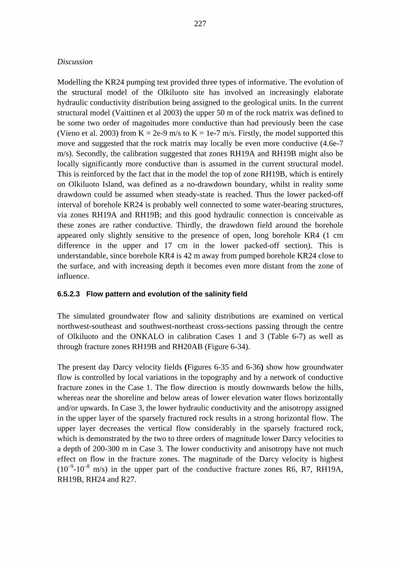
227

Discussion Modelling the KR24 pumping test provided three types of informative. The evolution of the structural model of the Olkiluoto site has involved an increasingly elaborate hydraulic conductivity distribution being assigned to the geological units. In the current structural model (Vaittinen et al 2003) the upper 50 m of the rock matrix was defined to be some two order of magnitudes more conductive than had previously been the case (Vieno et al. 2003) from K = 2e-9 m/s to K = 1e-7 m/s. Firstly, the model supported this move and suggested that the rock matrix may locally be even more conductive (4.6e-7 m/s). Secondly, the calibration suggested that zones RH19A and RH19B might also be locally significantly more conductive than is assumed in the current structural model. This is reinforced by the fact that in the model the top of zone RH19B, which is entirely on Olkiluoto Island, was defined as a no-drawdown boundary, whilst in reality some drawdown could be assumed when steady-state is reached. Thus the lower packed-off interval of borehole KR24 is probably well connected to some water-bearing structures, via zones RH19A and RH19B; and this good hydraulic connection is conceivable as these zones are rather conductive. Thirdly, the drawdown field around the borehole appeared only slightly sensitive to the presence of open, long borehole KR4 (1 cm difference in the upper and 17 cm in the lower packed-off section). This is understandable, since borehole KR4 is 42 m away from pumped borehole KR24 close to the surface, and with increasing depth it becomes even more distant from the zone of influence.

6.5.2.3 Flow pattern and evolution of the salinity field The simulated groundwater flow and salinity distributions are examined on vertical northwest-southeast and southwest-northeast cross-sections passing through the centre of Olkiluoto and the ONKALO in calibration Cases 1 and 3 (Table 6-7) as well as through fracture zones RH19B and RH20AB (Figure 6-34). The present day Darcy velocity fields (Figures 6-35 and 6-36) show how groundwater flow is controlled by local variations in the topography and by a network of conductive fracture zones in the Case 1. The flow direction is mostly downwards below the hills, whereas near the shoreline and below areas of lower elevation water flows horizontally and/or upwards. In Case 3, the lower hydraulic conductivity and the anisotropy assigned in the upper layer of the sparsely fractured rock results in a strong horizontal flow. The upper layer decreases the vertical flow considerably in the sparsely fractured rock, which is demonstrated by the two to three orders of magnitude lower Darcy velocities to a depth of 200-300 m in Case 3. The lower conductivity and anisotropy have not much effect on flow in the fracture zones. The magnitude of the Darcy velocity is highest (10–9-10–8 m/s) in the upper part of the conductive fracture zones R6, R7, RH19A, RH19B, RH24 and R27.

228

The evolution of the salinity field over the last 8000 years is illustrated in Figures 6-37 – 6-42. Initially, the upper part of the bedrock was assumed to be saturated with brackish groundwater, which is a mixture of subglacial groundwater and glacial meltwater. Deeper in the bedrock salinity increases and groundwater is composed of brackish and saline water layers, which follow the present measured values (see Chapter 6.3.2). At the beginning of the simulation, saline (Litorina) seawater starts to infiltrate the bedrock through the seabed. The higher concentration of seawater (12 g/l) results in a flow, which is driven purely by density differences, and this flow gradually mixes the recharging and deeper saline waters with the former brackish water. The mixing process is relatively fast along the fracture zones, due to their higher conductivity, compared with the sparsely fractured rock. In Case 3 the Litorina seawater infiltrates the bedrock only along these fracture zones, because of the lower conductivity and the anisotropy assigned to the upper layer of the sparsely fractured rock. Understandably, the nature of the infiltration in these fracture zones is similar in all the Cases. In Case 3 the infiltration of Litorina seawater may be too restricted. The quantity of Litorina-derived groundwater (actually 5-10 g/l) in the present situation appears to be insufficient at 100 to 250 m depth with an initial salinity 1 to 5 g/l, and the layer of 5 to 10 g/l initial salinity seem to endure almost undisturbed throughout the simulations; whereas in reality marine infiltration has generally reached 300 m depth. However, the inclusion of 1 to 5 g/l initial groundwater, which endures through simulations in the less transmissive parts of the upper bedrock, is in agreement with glacial reference groundwaters with no Litorina or younger signatures, which have been sampled at about 200 m depth. More information can be expected from future hydrogeochemical sampling of the poorly transmissive bedrock. Groundwater flow is driven purely by density differences until the highest hills on Olkiluoto Island rise above sea level about 3000-2500 years BP. This uplift causes fresh water to replace brackish and saline water below the widening area of the island (Figure 6-33). In Case 1 this fresh water not only forces brackish and saline water deeper into the bedrock, but in some areas also horizontally and upward. The system is generally diluted to 200 m depth, whereas in reality fresh groundwater should be clearly limited to depths of less than 100 m. In Case 3 the horizontal flow in the upper layer prevents the recharge of fresh water deeper into the bedrock, which corresponds well with hydrochemical observations. In fact, the anisotropy affects the flow and transport conditions so markedly that there are few changes in the sparsely fracture rock below the upper layer throughout the simulation. Only in the fracture zones does the fresh water penetrate to depths greater than 50 m (cf. Figures 6-39 and 6-40). Actually the flow simulation results for zone RH20AB are very similar to the salinity and initial water distributions modelled from the hydrogeochemical data (Figure 6-36). However, in the flow simulations dilution proceeds to a greater depth than that indicated by the groundwater samples, because the salinity approaches 5 to 10 g/l in the main zone of Litorina derived groundwater. This difference is similar to the results of zone RH19B,

229

as boreholes KR4 and KR8, which intersect this zone, show that groundwater is brackish. The penetration of fresh water into the zones is relatively fast in all the Cases, which is similar to the infiltration of Litorina sea water.

Figure 6-31. Measured and simulated salinity concentrations (TDS) along deep boreholes KR1-KR5 with the initial input parameters and in calibration cases 1-3 (Table 6-7).

230

Figure 6-32. Measured and simulated residual pressure along deep boreholes KR1-KR5 with the initial input parameters and in calibration cases 1-3 (Table 6-7).

231

Figure 6-33. The effect of land uplift on the salinity of the top boundary. The blue colour represents fresh water (the land above sea level), whilst the green denotes the salinity of the present sea water (5.6 g/l).

232

Figure 6-34. Modelled volume and location of the cross-sections, along which the salinities and Darcy velocities are presented.

233

Figure 6-35. The present day Darcy velocity field along the vertical cross-sections (see Figure 6-34) in calibration case 1.

234

Figure 6-36. The present day Darcy velocity field along the vertical cross-sections (see Figure 6-34) in calibration case 3 (Table 6-7).

235

Figure 6-37. Evolution of groundwater salinity along the vertical northwest-southeast cross-section (see Figure 6-34) in calibration case 1 (Table 6-7).

236

Figure 6-38. Evolution of groundwater salinity along the vertical southwest-northeast cross-section (see Figure 6-34) in calibration case 1 (Table 6-7).

237

Figure 6-39. Evolution of groundwater salinity along the vertical northwest-southeast cross-section (see Figure 6-34) in calibration case 3 (Table 6-7).

238

Figure 6-40. Evolution of groundwater salinity along the vertical southwest-northeast cross-section (see Figure 6-34) in calibration case 3 (Table 6-7).

239

Figure 6-41. Evolution of groundwater salinity in fracture zone RH19B in calibration case 3 (Table 6-7).

240

Figure 6-42. Evolution of groundwater salinity in fracture zone RH20AB in calibration case 3 (Table 6-7).

241

6.6 Evaluation of uncertainties and sensitivities

6.6.1 Hydrogeology The numerical modelling of groundwater flow and solute transport is subject to large uncertainties relating to the input parameters. The structural geometry of the hydrogeological model and the transmissivity of the zones (discussed in detail at the end of this section), as well as the hydraulic conductivity of the sparsely fractured rock, constitute the largest uncertainties in the simulations. The hydraulic conductivities of the sparsely fractured rock measured in the cored boreholes show a considerable variation. Because this rock is conceptually modelled as a porous medium, which requires a relatively simple representation of the hydraulic conductivity, the measured small-scale hydraulic conductivities are averaged in order to obtain conductivities that represent a similar overall behaviour of the network of fractures on a larger length scale. This process, which resulted in five different depth layers for the conductivity (Chapter 6.3.2), is obviously subject to considerable uncertainties. The initial state of the salinity distribution at the Litorina stage is based on the hydrogeochemical interpretations, with the applied model being a simple, depth-dependent curve. Although the calibration indicated that the simulated present day salinities were not sensitive to small changes in their initial state, it is clear that the initial salinity field should be spatially variable, although the extent of this variability is poorly known. For example, hydrogeochemical data suggest that the salinity gradient is more gentle around borehole KR3 than elsewhere at the site (see Figure 6-31). The lower limit of saline water (10 g/l) is hardly reached in borehole KR3, which is in contrast to observations from other boreholes, in which values of about 15 g/l are seen. In addition to the aforementioned factors, the flow porosity and dispersion length constitute a source of uncertainty from the point of view of solute transport, as there are no experimental data available for these parameters. The flow porosity affects the time scales of solute transport, whilst the main effect of dispersion is on the spreading of the concentration front. An increase in the flow porosity of one order of magnitude and a decrease in the dispersion length from 50 to 30 m resulted in slightly higher present day salinities compared with the initial values (see calibration in Section 6.5.2). Thus, the present day salinity seems not to be sensitive to the values of flow porosity and dispersion. It was not possible to include a thorough sensitivity analysis in this study, in order to keep the amount of modelling work to a reasonable level. The simulated pressure was relativ insensitive to the changes made in the calibration, although Case 3, (Table 6-7) with lower hydraulic conductivity and anisotropy, gave somewhat better results that the other cases. However, the pressures, as well as the salinities, were sensitive to the conceptual fracture zone geometry.

242

6.6.1.1 Conceptual fracture zone geometry The conceptual fracture zone geometry constitutes one of the main sources of uncertainty in the site-scale groundwater flow analyses. The geometry is based on the bedrock model, which is a descriptive model of the actual bedrock and consists of all the geological, geophysical and hydrogeological knowledge gathered from the field investigations carried out for the Olkiluoto site. The bedrock model has undergone several changes due to the continuing investigations and interpretations, which have resulted in the introduction of several new fracture zones, as well as modifications to the properties and geometries of many existing zones. Whilst the bedrock model is a simplification of the real bedrock, the conceptual fracture zone geometry in the groundwater flow model is a simplification of the bedrock model. Typically the bedrock model contains several tens of fracture zones of various dimensions and transmissivities. However, from a point of view of site-scale groundwater flow, the presence of isolated disks and zones of limited extent (and low transmissivity), which do not intersect other zones and, therefore, do not constitute important flow routes, are not included in the flow model explicitly, but are taken into account implicitly in the hydraulic conductivity of the sparsely fractured rock between the zones. On the other hand, many fracture zones that are weakly connected or very close to each other are extended so as to intersect each other. Although the conceptual fracture zone geometry in the flow model is a simplified and revised version of the bedrock model, a special emphasis has been placed on preserving the essential hydrogeological similarities of the models. The groundwater flow analyses by Koskinen (1992, 1995) and Löfman (1996) were based on the bedrock model by Saksa et al. (1993), whereas Löfman (1999, 2000) employed the bedrock model of Saksa et al. (1998). The latest flow analysis dealing with the hydraulic disturbance of the ONKALO (Vieno et al. 2003) was based on the bedrock model of Saksa et al. (2002). The current analysis applies the hydrogeological model and correlated structures of the structural model of the latest bedrock model, version 2003/1 (Vaittinen et al. 2003) (see Section 6.2.1). The geometries in the flow model and the corresponding bedrock models are summarised in Table 6-8. This discussion aims at illustrating the effects of alternative fracture zone geometries by using the four geometries mentioned above. Apart from the geometry and the corresponding transmissivities, everything else in the flow models (i.e. hydraulic conductivities, initial and boundary conditions, etc.) are the same as those used in the current flow model. Simulated residual pressures along deep boreholes KR1-KR5 are presented in Figure 6-43, which shows that the pressures are clearly sensitive to the geometry assigned to the fracture zones. The best agreement with the field data is obtained using the

243

geometry of the 1999 model (Table 6-8), whereas the current geometry of the 2004 model gives the worst agreement, with the geometries of the 1992 and 2004 models lying somewhere in between. The sensitivity of the results to the geometry is also demonstrated by the simulated salinities along the deep boreholes (Figure 6-44). Although it is difficult to judge whether a particular geometry is better than another from an analysis of the field data, it is possible to examine such differences between the various geometries in the simulated salinities in boreholes (e.g. in borehole KR3 and KR4) which intersect fracture zones; and these differences are considerable.

The fracture zone geometries of the 1992, 2003 and 2004 models (Table 6-8) were constructed from the bedrock models in a relatively simple and straightforward manner, as described above. The geometry of the 1999 model, however, took advantage of the results from the hydrogeological field investigations (pumping tests and measured pressures in deep boreholes), which offered considerable information about hydrogeological connections (fracture zones) which were not documented in the bedrock model. Consequently, some fracture zones, which consisted of several disks or zones with a limited extent, were connected so as to produce larger, continuous zones. The fracture zone geometry was, therefore, quite different from that of the original bedrock model. The main difference between the geometry of the 1999 model and the other models is that it consists of a smaller number of zones which are, however, more extensive and better connected with other zones (Figures 6-45 and 6-46). In particular, the geometry of the 1999 model contains several zones oriented in a southwest-northeast direction, which extend across the island to the sea or to areas of lower elevation, which is one reason for a good agreement between the measured and simulated pressures in the boreholes. Although the continuing site investigations and interpretations have resulted in evolving bedrock and flow models, the overall conception of the flow conditions at Olkiluoto has not changed. This discussion indicates, however, that the groundwater flow simulations are sensitive to the conceptual fracture zone geometries assumed, at least locally to the boreholes. Special attention should be placed, therefore, on the construction of bedrock and flow models, in which advantage should be taken of all the available hydrogeological data. Table 6-8. Flow models and corresponding bedrock models employed in the groundwater flow analyses at Olkiluoto since 1992.

Conceptual fracture zone geometry in the flow model

Bedrock model

1992: Koskinen (1992, 1995), Löfman (1996) Saksa et al. (1993) 1999: Löfman (1999, 2000) Saksa et al. (1998) 2003: Vieno et al. (2003) Saksa et al. (2002) 2004: Current model Vaittinen et al. (2003)

244

Figure 6-43. Measured and simulated residual pressures along deep boreholes KR1-KR5.

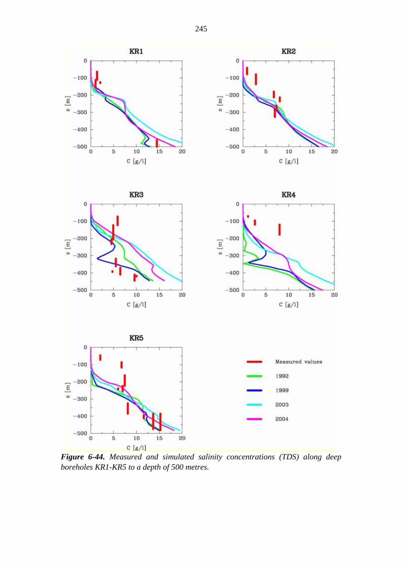
245

Figure 6-44. Measured and simulated salinity concentrations (TDS) along deep boreholes KR1-KR5 to a depth of 500 metres.

246

Figure 6-45. The conceptual fracture zone geometry used in the current model (see Table 6-8).

Figure 6-46. The conceptual fracture zone geometry of the 1999 model (see Table 6-8).

247

6.6.2 Hydrogeochemistry

The model of the hydrogeochemical evolution of Olkiluoto is sensitive to uncertainties related to chemical data, to the representivity of the samples and to the interpreted concept of the water-rock interactions. Single groundwater samples may be subject to measurement uncertainties, to problems during sampling and to hydrogeological problems in sampling sections. This last problem may be due to, for example, to strong internal flow in an open borehole, to biased sampling due to heterogeneous hydraulic properties, to the mixing of different groundwaters due to hydraulic connections and to seasonal variations.

The uncertainties associated with single groundwater samples have decreased, due to an increase in the database, due to the development of a denser sampling network, and by repeating sampling in single sections at different times. The presence of this denser sampling network has also decreased uncertainties related to the evaluation of the dominant processes that influence the hydrochemical conditions, such as redox processes involving microbes. Occasional inconsistencies in the data can be observed by comparing the data internally, as has been done in the evaluation of the hydrochemical baseline data by Hellä et al. (2005). An evaluation has also been carried out of the uncertainties caused by the hydrogeological conditions in sampling sections. All groundwater samples taken during the baseline site investigation have been graded, in order to increase the reliability of the hydrochemical data and to minimise uncertainties for further interpretations.

It is also important to understand when considering the reliability of single data points, that they are not applied to represent hydrochemical conditions at too detailed a scale. On the other hand, using the whole database effectively averages the conditions between the data points, whereas the chemical conditions are in fact spatially variable, particularly in poorly conductive parts of the rock where no groundwater samples are available. The salinity does not, however, seem to depend on the hydraulic conductivity of fractures, which increases the reliability of the hydrogeochemical concept. The extent of hydrochemical variation in tight, diffusion-controlled parts of the bedrock still remains uncertain, although the long residence times for groundwater at depth where salinities are high suggest that salinity differences between fractures and this tight rock may be limited. In the upper part of the bedrock, which has been subject to dynamic conditions since glacial times, due to the influx of glacial water, Litorina and currently meteoric water, hydrochemical differences are more probable between the more and less transmissive parts of the bedrock.

There is a significant uncertainty in defining the initial conditions at the site at the start of the model presented in Section 6.5.2, in particular the salinity of the subglacial groundwater in the upper part of the bedrock. The model assumes that this subglacial groundwater is present at depths greater than 100 to 150 m, i.e. below the HCO3-rich groundwater. The estimated salinity of this subglacial groundwater is sensitive to the

248

estimated salinity of the pre-Litorina groundwater, which in turn depends on the Litorina seawater fraction, as shown in Chapter 6.3.1. The range of Cl concentrations in pre-Litorina groundwater (1750 ± 600 mg/l) indicates a corresponding range from 2300 to 4700 mg/l in subglacial groundwater. However, the Cl concentration cannot be less than 3000 mg/l, otherwise the glacial meltwater component would disappear from glacial reference samples (i.e. only pure subglacial water would be present). If the concentration increases significantly, the glacial meltwater fraction in mixing models would also increase, which would decrease considerably the theoretical 18O values in brackish and saline groundwater samples.

Figure 6-47 shows the sensitivity of Cl concentration in subglacial initial water to the theoretical 18O-values of groundwater samples. The values are calculated according to initial water mixing based on mass-balance models, assuming 18O-values to be -11.5, -4.7, -20, -12 and -11‰ for meteoric, Litorina, glacial, subglacial and saline initial waters, respectively. Oxygen-18 is mainly an independent parameter in the mixing models (it is used in only a few models, see Pitkänen et al. 1999, 2004) and can therefore be used in this sensitivity analysis. Theoretical values of 18O with Cl concentrations of 3000 to 3500 mg/l fit fairly well with measured values, whereas when Cl concentrations reach 5000 mg/l in subglacial initial water, 18O decreases and deviates significantly from measured values. The results suggest that Cl concentrations would have been somewhat below, rather than above, 3500 mg/l in subglacial groundwater and that the calculated fractions of glacial meltwater in groundwater samples represent maximum values.

249

Figure 6-47. Comparison of theoretical and measured 18O-values for groundwater samples at Olkiluoto. Theoretical values are calculated according to mass-balance models from initial waters.

A major drawback related to the 3-D hydrogeochemical illustrations is related to the limited number of good quality groundwater samples. The characterisation of the extensive WCA volume (total volume is 3.6 km3) is carried out with 93 quality evaluated samples. It is inevitable that this kind of generalisation of the baseline conditions is unable to take into account all of the local heterogeneities, although the secondary centroid network is a tool for making local adjustments. There are also significant volumes within the WCA without an observation-based definition of the distribution of the water types as a function of depth (i.e. the areas below the Baltic Sea).

The 3-D hydrogeochemical illustrations rely on two basic aspects: that a quality evaluated sample is an indication of broader characteristics within bedrock and that the majority of the groundwater that moves within the bedrock is located in the fracture zones. The observed layering of initial waters within the WCA volume (cf.

250

Figures 6-19 to 6-22) suggests that the first assumption is correct. The second assumption is intuitively correct when considering the differences in transmissivity between the fracture zones and the less fractured parts of the bedrock (cf. also Figure 6-6b). The 3-D illustration approach is, thus, a method that averages the observed hydrogeochemistry over unknown volumes of bedrock.

It is likely, however, that the 3-D hydrogeochemical illustrations fail to take into account the mutual and internal heterogeneities of the fracture zones and, in the baseline conditions, these effects remain largely hidden. The slow post-glacial land uplift has had a tendency to favour the smooth layering of initial waters within the fracture zones. During the open tunnel phase of the ONKALO it is expected that the high hydraulic gradients generated will bring out the differences in the transmissivities of the fracture zones, and also the anisotropies within single fracture zones. Any illustration of these features using 3-D hydrogeochemical mapping will necessarily be incomplete, because it will not be possible to obtain sufficient geochemical data.

The 3-D hydrogeochemical visualisation will, therefore, likely remain as an averaging method in the future, for the reasons given above. The benefit of the method is its use as a mapping tool, which will allow the increasing number of geochemical samples to be summarised and compared with each other, and for the interpretations to be visualised without presenting the results of single geochemical samples.

In addition, information other than that of a purely hydrogeochemical nature could be included as part of the hydrogeochemical illustrations. As an example, electrical conductivity measurements are produced in much greater numbers than hydrogeochemical samples, and the skilled use of such data could contribute significantly to the details of the hydrogeochemical 3-D illustrations.

6.7 Discussion The integration of hydrogeochemistry and flow simulations is a laborious, time-consuming and iterative process. The progress towards consistent models has developed, though has not been completely achieved. The iterative approach used is based on the method of trial and error, in which the results of flow simulations (pressure and salinity) are calibrated against the measured values by adjusting several input parameters. Progress can vary in this process of adjustment from minor to significant, with occasional phases when the calibration process goes into reverse; and it was not possible to obtain complete consistency during the time available. On the other hand, it is unrealistic to expect to obtain perfect consistency due to uncertainties and necessary simplifications included in the geological, hydrogeological and hydrogeochemical models. It should be possible, however, to demonstrate, and possibly correct, any clear contradictions between disciplines, or at least provide plausible reasons for such differences - for example, strongly divergent simulated and measured pressure values or simulated fresh water infiltration into volumes of bedrock which actually contain brackish groundwater which shows an extended residence time.

251

There was a significant improvement, in comparison with the EQUIP project (e.g. Gehör et al. 2001), in the consistency achieved between the salinity distributions obtained from the flow simulations and the hydrogeochemistry. This correspondence is fairly good in Case 3 when using an anisotropic hydraulic conductivity in the upper 50 m and a decreased conductivity distribution in the bedrock. Fresh water infiltration is generally confined to well above 100 m in the bedrock (Figures 6-31, 6-39, 6-40), as is also indicated by the hydrogeochemical model, whereas the upper 300 m was totally diluted in the previous model. However, in comparison with the hydrochemical observations, fresh water still infiltrates (in all the simulated cases) to too great a depth along certain transmissive structures, such as RH19B, suggesting that the hydraulic properties of highly conductive zones need to be investigated further. The infiltration of Litorina seawater to depths of between 100 to 300 m seems not to reach the volumes indicated by hydrogeochemical data, which may be due to the way in which the hydraulic data have been parameterised. On the hand, the reason that this infiltration remains too restricted may also be due to the hydrostructural model itself, which may not contain a sufficient number of adequately transmissive and hydraulically connected structures. Such structures would be needed to allow marine infiltration over several thousands of years and to allow buffering of the marine derived groundwater against meteoric infiltration over the last thousands of years. This and the fact that the results were sensitive to the structural model, indicate that special attention should be placed on the construction of the bedrock and flow models. The integration process (cf. Figure 6-18) should be continued during the next evaluation round, i.e. during the preparation of the Site Report for 2006, when the data gained from the ONKALO may allow a better representation of the hydrogeological properties of the upper part of the bedrock. This would also increase confidence in predicting the hydrogeological evolution of both the ONKALO and in the development of the Safety Case for Olkiluoto.

123 5 rock mechanics this chapter describes the rock - posiva

Documents