© alchemyapi ceng 501 deep learning week 8
TRANSCRIPT

CENG 501 Deep Learning
Week 8
Sinan Kalkan
© AlchemyAPI

Representational Capacity• More hidden neurons è capacity to represent more complex functions
• Problem: overfitting vs. generalization– We will discuss the different strategies to help here (L2 regularization, dropout, input noise, using a
validation set etc.)
2
Figure: https://cs231n.github.io/
Previously on CENG501!
Spring 2021 Sinan Kalkan

Number of hidden layers
• Depends on the nature of the problem– Linear classification? è No hidden layers needed– Non-linear classification?
3
Previously on CENG501!
Spring 2021 Sinan Kalkan

What do the layers represent?
Spring 2021 Sinan Kalkan 4
Trainable Classifier
Low-LevelFeature
Mid-LevelFeature
High-LevelFeature
Feature visualization of convolutional net trained on ImageNet from [Zeiler & Fergus 2013]
“car”Previously
on CENG501!

Model Complexity• Models range in their flexibility to fit arbitrary data
complex model
unconstrained
large capacity mayallow it to memorizedata and fail tocapture regularities
simple model
constrained
small capacity mayprevent it from representing allstructure in data
low bias
high variance
high bias
low variance
Slide Credit: Michael Mozer
5
Previously on CENG501!
Spring 2021 Sinan Kalkan

Training Vs. Test Set Error
Test Set
Training Set
Slide Credit: Michael Mozer 6
Previously on CENG501!
Spring 2021 Sinan Kalkan

Avoiding Overfitting
• Increase training set size– Make sure effective size is growing; redundancy doesn’t help
• Incorporate domain-appropriate bias into model– Customize model to your problem
• Set hyperparameters of model– number of layers, number of hidden units per layer, connectivity, etc.
• Regularization techniques
Slide Credit: Michael Mozer7
Previously on CENG501!
Spring 2021 Sinan Kalkan

Regularization
• L2 regularization: !"𝜆𝑤"
– Very common– Penalizes peaky weight vector, prefers diffuse weight vectors
• L1 regularization: 𝜆|𝑤|– Enforces sparsity (some weights become zero)– Why? Weight decay is by a constant value if |w| is non-zero.– Leads to input selection (makes it noise robust)– Use it if you require sparsity / feature selection
• Can be combined: 𝜆! 𝑤 + 𝜆"𝑤"
• Regularization is not performed on the bias; it seems to make no significant difference
8
Previously on CENG501!
Spring 2021 Sinan Kalkan

Regularization
• Enforce an upper bound on weights:– Max norm:
• 𝑤 ! < 𝑐• Helps the gradient explosion problem• Improvements reported
• Dropout:– At each iteration, drop a number of
neurons in the network– Use a neuron’s activation with
probability 𝑝 (a hyperparameter)– Adds stochasticity!
http://cs231n.github.io/neural-networks-2/
Fig: Srivastava et al., 2014
9
Previously on CENG501!
Spring 2021 Sinan Kalkan

Regularization: Inverted Dropout
Test-time:
Training-time: Correct the expected expected output from 𝑝𝑥 to 𝑥.
http://cs231n.github.io/neural-networks-2/
Perform scaling while dropping at training time!
10
Previously on CENG501!
Spring 2021 Sinan Kalkan

Dropout as Ensemble Training Method
“Dropout performs gradient descent on-line with respect to both the training examples and the ensemble of all possible subnetworks.”
Spring 2021 Sinan Kalkan 11
Pierre Baldi and Peter J Sadowski. Understanding dropout. In Advances in neural information processing systems, pp. 2814–2822, 2013.
Fig: Srivastava et al., 2014Previously on CENG501!
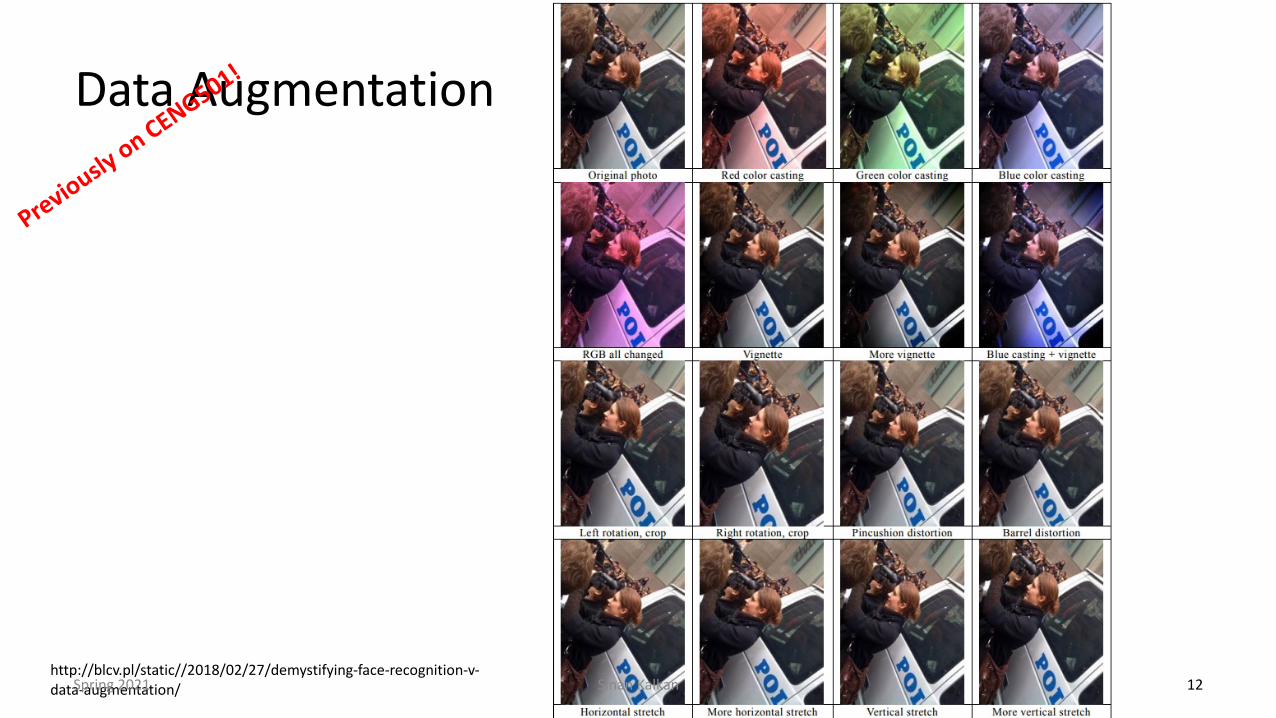
Data Augmentation
12http://blcv.pl/static//2018/02/27/demystifying-face-recognition-v-data-augmentation/
Previously on CENG501!
Spring 2021 Sinan Kalkan

When to stop training: Early stopping
Slide Credit: Michael Mozer13
Test Set
Training Set
Previously on CENG501!
Spring 2021 Sinan Kalkan

Data Preprocessing: Mean subtraction• Compute the mean of each dimension, 𝜇!, over the training set:
𝜇! =1𝑁&"
𝑥"!
• Subtract the mean for each dimension:𝑥′"! ← 𝑥"! − 𝜇!
• Effect: Move the data center (mean) to coordinate center
http://cs231n.github.io/neural-networks-2/14
Mean image of CIFAR10(from PA1)
Previously on CENG501!
Spring 2021 Sinan Kalkan

Data Preprocessing: Normalization (or conditioning)
• Necessary if you believe that your dimensions have different scales– Might need to reduce this to give equal importance to each dimension
• Normalize each dimension by its std. dev. after mean subtraction:𝑥"!# = 𝑥"! − 𝜇!𝑥"!## = 𝑥"!# /𝜎!
• Effect: Make the dimensions have the same scale
http://cs231n.github.io/neural-networks-2/15
Previously on CENG501!
Spring 2021 Sinan Kalkan

Initial Weight Normalization
• Problem: Variance of the output changes with the number of inputs
• If 𝑠 = ∑!𝑤!𝑥! (note that 𝑉𝑎𝑟(𝑋) = 𝐸 𝑋 − 𝜇 " ):
16Eqn: https://cs231n.github.io/neural-networks-2/#init
Previously on CENG501!
Spring 2021 Sinan Kalkan

Initial Weight Normalization
• Solution:– Getridof𝑛 in𝑉𝑎𝑟 𝑠 = (𝑛Var(w))Var(x)
• How?– Scale the initial weights by 𝑛– Why? Because: 𝑉𝑎𝑟 𝑎𝑋 =𝑎!𝑉𝑎𝑟 𝑋
• Standard Initialization (top plots in Figure 6 & 7):
𝑤" ∼ 𝑈 −1𝑛,1𝑛
which yields 𝑛 𝑉𝑎𝑟 𝑤 = #$
because variance of 𝑈[−𝑟, 𝑟] is %!
$.
17
Figures: Glorot & Bengio, “Understanding the difficulty of training deep feedforward neural networks”, 2010.
Xavier initialization for symmetric activation functions (Glorot & Bengio):
𝑤" ∼ 𝑁 0,2
𝑛"& + 𝑛'()
With Uniform distribution:
𝑤" ∼ 𝑈 −6
𝑛"& + 𝑛'(),
6𝑛"& + 𝑛'()Spring 2021 Sinan Kalkan
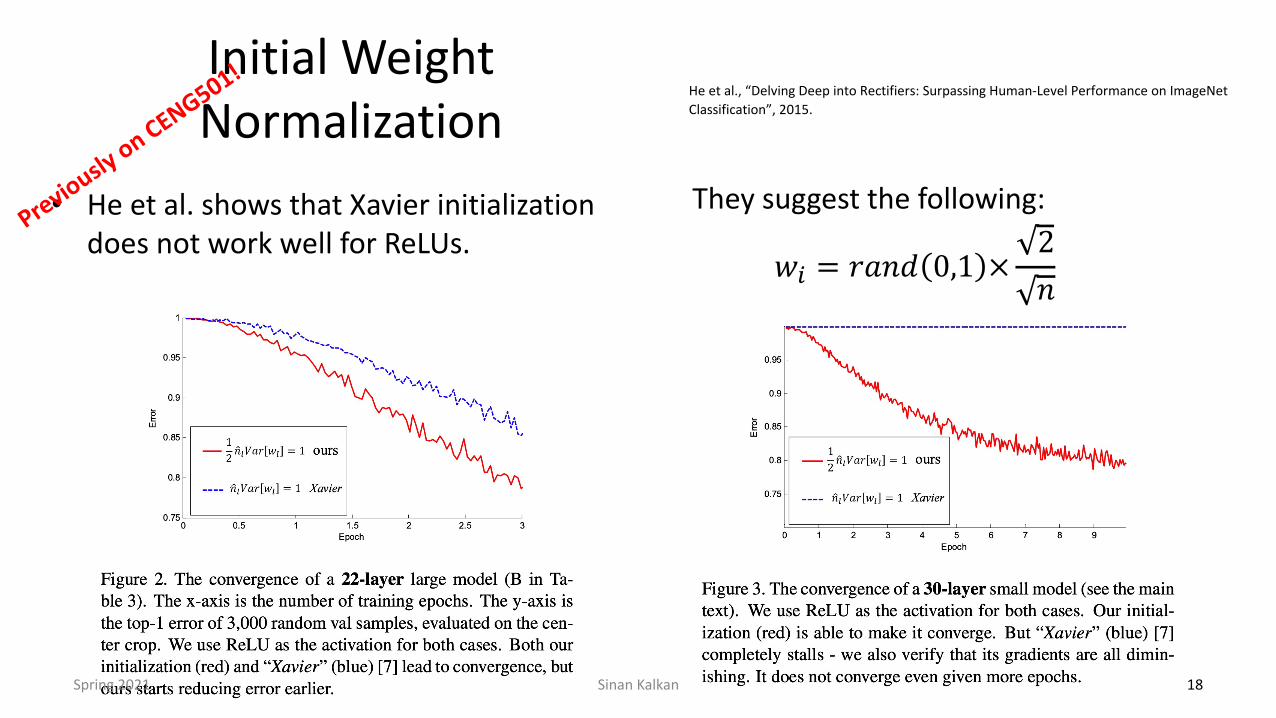
Initial Weight Normalization
• He et al. shows that Xavier initialization does not work well for ReLUs.
18
He et al., “Delving Deep into Rectifiers: Surpassing Human-Level Performance on ImageNet Classification”, 2015.
They suggest the following:
𝑤M = 𝑟𝑎𝑛𝑑 0,1 ×2𝑛
Previously on CENG501!
Spring 2021 Sinan Kalkan

More on Weight Initialization
Tutorial and Demo:https://www.deeplearning.ai/ai-notes/initialization/index.html
Tutorial:https://mmuratarat.github.io/2019-02-25/xavier-glorot-he-weight-init
Spring 2021 Sinan Kalkan 19

Alternative: Batch Normalization• Normalization is differentiable
– So, make it part of the model (not only at the beginning)
– I.e., perform normalization during every step of processing
• More robust to initialization• Shown to also regularize the network in
some cases (dropping the need for dropout)• Issue: How to normalize at test time?
1. Store means and variances during training, or
2. Calculate mean & variance over your test data
• PyTorch: use model.eval() in test time.Ioffe & Szegedy, “Batch Normalization: Accelerating Deep Network Training by Reducing Internal Covariate Shift”, 2015.
20
Previously on CENG501!
Spring 2021 Sinan Kalkan
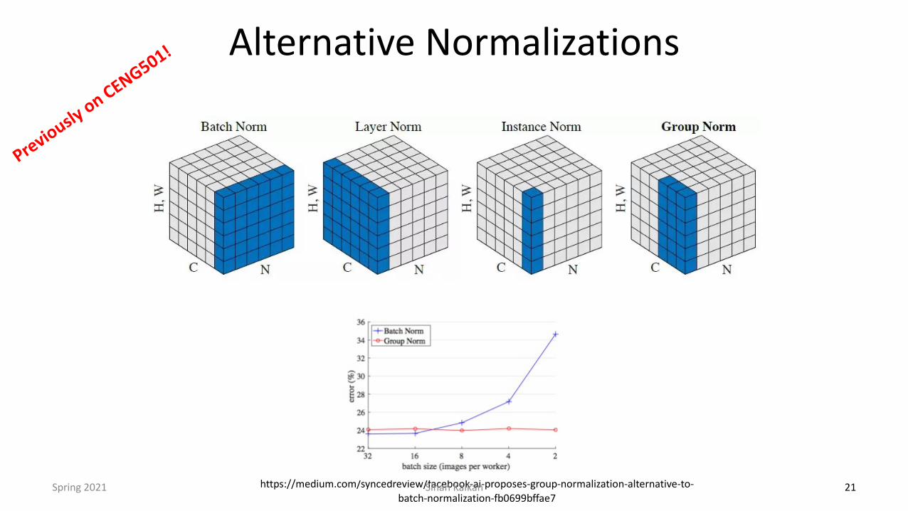
Alternative Normalizations
21https://medium.com/syncedreview/facebook-ai-proposes-group-normalization-alternative-to-batch-normalization-fb0699bffae7
Previously on CENG501!
Spring 2021 Sinan Kalkan

22
2018
Previously on CENG501!
Spring 2021 Sinan Kalkan

What if things are not working?
Learning rate might be too low; Batch size might be too small
23
Previously on CENG501!
Spring 2021 Sinan Kalkan
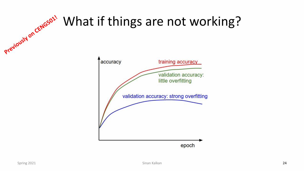
What if things are not working?
24
Previously on CENG501!
Spring 2021 Sinan Kalkan

Today• Convolutional Neural Networks
– Disadvantages of MLPs– Advantages of CNNs– CNN Operations: Convolution, pooling, nonlinearity, normalization, FC– CNN Architectures:
• Next week:– Backpropagation with a CNN– Transfer learning– Visualizing and understanding CNNs– Widely-used CNN architectures– CNN Applications
Spring 2021 Sinan Kalkan 25
These slides available at: http://kovan.ceng.metu.edu.tr/~sinan/DL/week_8.pdf

Administrative Issues
• Programming assignment 1
• Take-Home Exam 1:– Announced: 3rd of May– Deadline: 9th of May?
• Project paper selection– https://docs.google.com/spreadsheets/d/1tzPHq_Vgu6gCwNyXJHGvqeA6p
gU67H0nKYjqkisWfKc/edit?usp=sharing– Deadline: 19th of April
Spring 2021 Sinan Kalkan 26

CONVOLUTIONAL NEURAL NETWORKS: MOTIVATION
27Spring 2021 Sinan Kalkan

Disadvantages of MLPs: Curse of Dimensionality
• Number of required samples for obtaining small error increases exponentially with input dimensions
• Too many many parameters
Spring 2021 Sinan Kalkan 28
https://towardsdatascience.com/geometric-foundations-of-deep-learning-94cdd45b451d

Disadvantages of MLPs: Equivariance
• Vectorizing an image breaks patterns in consecutive pixels. – Shifting one pixel means a whole new vector– Makes learning more difficult – Requires more data to generalize
Spring 2021 Sinan Kalkan 29Figure: http://cs231n.github.io/linear-classify/

Equivariance vs. Invariance
• Equivariant problem: image segmentation. – f(g(x)) = g(f(x))
• Invariant problem: object recognition. – f(g(x)) = f(x)
• Pooling provides invariance, convolution provides equivariance.
Spring 2021 Sinan Kalkan 30
https://www.mathworks.com/discovery/image-segmentation.html
f(x): “cat” f(g(x)): “cat”
g(x)

An Alternative to MLPs
Solution (inspiration): • Hubel & Wiesel: Brain neurons are not fully connected. They have local receptive fields
Spring 2021 31http://fourier.eng.hmc.edu/e180/lectures/retina/node1.html
Sinan Kalkan

An Alternative to MLPsSolution: Neocognitron (Fukushima, 1979):
A neural network model unaffected by shift in position, applied to Japanese handwritten character recognition.
• S (simple) cells: local feature extraction.• C (complex) cells: provide tolerance to
deformation, e.g. shift.• Self-organized learning method.
Spring 2021 Sinan Kalkan 32
Figure: Fukushima (2019), Recent advances in the deep CNN neocognitron.

An Alternative to MLPs
Solution: Neocognitron’s self-organized learning method (Fukushima, 2019):
Spring 2021 Sinan Kalkan 33
“For training intermediate layers of the neocognitron, the learning rule called AiS (Add-if-Silent)is used. Under the AiS rule, a new cell is generated and added to the network if all postsynapticcells are silent in spite of non-silent presynaptic cells. The generated cell learns the activity of thepresynaptic cells in one-shot. Once a cell is generated, its input connections do not change any more.Thus the training process is very simple and does not require time-consuming repetitive calculation.”

An Alternative to MLPs
Solution: Convolutional Neural Networks (Lecun, 1998)– Gradient descent– Weights shared– Document recognition
Spring 2021 Sinan Kalkan 34

CNNs: Underlying Principle
Spring 2021 Sinan Kalkan 35
Figure: Goodfellow et al., “Deep Learning”, MIT Press, 2016.

CNNs vs. MLPs: Curse of Dimensionality
• A fully-connected network has too many parameters– On CIFAR-10:
• Images have size 32x32x3 è one neuron in hidden layer has 3072 weights!
– With images of size 512x512x3 è one neuron in hidden layer has 786,432 weights!
– This explodes quickly if you increase the number of neurons & layers.
• Alternative: enforce local connectivity!Figure: Goodfellow et al., “Deep Learning”, MIT Press, 2016.
Spring 2021 Sinan Kalkan 36

When things go deep, an output may depend on all or most of the input:
Figure: Goodfellow et al., “Deep Learning”, MIT Press, 2016.
CNNs vs. MLPs: Curse of Dimensionality
Spring 2021 Sinan Kalkan 37

Motivation
Spring 2021 Sinan Kalkan 38

• Parameter sharing– In regular ANN, each weight is independent
• In CNN, a layer might re-apply the same convolution and therefore, share the parameters of a convolution– Reduces storage and learning time
• For a neuron in the next layer:– With ANN: 320x280x320x280 multiplications– With CNN: 320x280x3x3 multiplications
320x280320x280
Figure: Goodfellow et al., “Deep Learning”, MIT Press, 2016.
CNNs vs. MLPs: Curse of Dimensionality
Spring 2021 Sinan Kalkan 39

• Equivariant to translation– The output will be the same, just translated, since the weights are shared.
• Not equivariant to scale or rotation.
Figure: https://towardsdatascience.com/translational-invariance-vs-translational-equivariance-f9fbc8fca63a
CNNs vs. MLPs: Equivariance
Spring 2021 Sinan Kalkan 40

A CRASH COURSE ON CONVOLUTION
Spring 2021 Sinan Kalkan 41

Spring 2021 Sinan Kalkan 42
Formulating Signals in Terms of Impulse Signal

Formulating Signals in Terms of Impulse Signal
Spring 2021 Sinan Kalkan 43

Unit Sample Response
Spring 2021 Sinan Kalkan 44

Conclusion
Spring 2021 Sinan Kalkan 45

Power of convolution
• Describe a “system” (or operation) with a very simple function (impulse response).
• Determine the output by convolving the input with the impulse response
Spring 2021 Sinan Kalkan 46
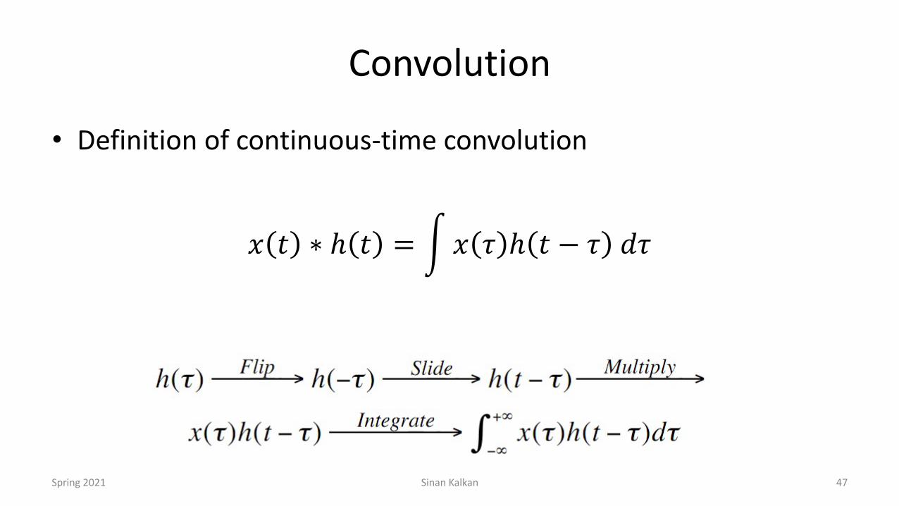
Convolution
• Definition of continuous-time convolution
𝑥 𝑡 ∗ ℎ 𝑡 = 2𝑥 𝜏 ℎ 𝑡 − 𝜏 𝑑𝜏
Spring 2021 Sinan Kalkan 47

Convolution• Definition of discrete-time convolution
𝑥[𝑛] ∗ ℎ[𝑛] =&𝑥 𝑘 ℎ[𝑛 − 𝑘]
Spring 2021 Sinan Kalkan 48

Discrete-time 2D Convolution
• For images, we need two-dimensional convolution:
• These multi-dimensional arrays are called tensors• We have commutative property:
• Instead of subtraction, we can also write (easy to drive by a change of variables). This is called cross-correlation:
Spring 2021 Sinan Kalkan 49

Example multi-dimensional convolution
Spring 2021 Sinan Kalkan 50
Figure: Goodfellow et al., “Deep Learning”, MIT Press, 2016.
https://github.com/vdumoulin/conv_arithmetic

What can filters do? Rectangular filter
Ä
g[m,n]
h[m,n]
=
f[m,n]
Slide: A. Torralba

What can filters do? Rectangular filter
Ä
g[m,n]
h[m,n]
=
f[m,n]
Slide: A. Torralba

What can filters do? Rectangular filter
Ä
g[m,n]
h[m,n]
=
f[m,n]
Slide: A. Torralba

What can filters do? Sharpening filter
coef
ficie
nt
-0.35original
8
Sharpened(differences are
accentuated; constantareas are left untouched).
1.7
filter
11.2
-0.25
8
result
Slide: A. Torralba

What can filters do? Sharpening filter
before after
Slide: A. Torralba

What can filters do? Gaussian filter
s=1
s=2
s=4
Slide: A. Torralba

Global to Local Analysis
Dali
Slide: A. Torralba

What can filters do?[-1 1]
Ä
g[m,n]
h[m,n]
=
f[m,n]
[-1, 1]
Slide: A. Torralba

What can filters do?[-1 1]T
Ä
g[m,n]
h[m,n]
=
f[m,n]
[-1, 1]T
Slide: A. Torralba

OVERVIEW OF CNN
Spring 2021 Sinan Kalkan 60

CNN layers
• Stages of CNN:– Convolution (in parallel) to produce pre-synaptic
activations– Detector: Non-linear function– Pooling: A summary of a neighborhood
• Pooling of a rectangular region:– Max– Average– L2 norm– Weighted average acc. to the distance to the
center– …
Figure: Goodfellow et al., “Deep Learning”, MIT Press, 2016.Spring 2021 Sinan Kalkan 61

An example architecture
http://cs231n.github.io/convolutional-networks/Spring 2021 Sinan Kalkan 62

Regular ANN
CNN
http://cs231n.github.io/convolutional-networks/Spring 2021 Sinan Kalkan 63

OPERATIONS IN A CNN: CONVOLUTION
Spring 2021 Sinan Kalkan 64

Convolution in CNN
• The weights correspond to the kernel
• The weights are shared in a channel (depth slice)
• We are effectively learning filters that respond to some part/entities/visual-cues etc.
Figure: Goodfellow et al., “Deep Learning”, MIT Press, 2016.Spring 2021 Sinan Kalkan 65

Local connectivity in CNN = Receptive fields
• Each neuron is connected to only a local neighborhood, i.e., receptive field• The size of the receptive field è another hyper-parameter.
Spring 2021 Sinan Kalkan 66

Connectivity in CNN
http://cs231n.github.io/convolutional-networks/
• Local: The behavior of a neuron does not change other than being restricted to a subspace of the input.
• Each neuron is connected to slice of the previous layer • A layer is actually a volume having a certain width x height and depth (or channel)• A neuron is connected to a subspace of width x height but to all channels (depth)• Example: CIFAR-10
– Input: 32 x 32 x 3 (3 for RGB channels)– A neuron in the next layer with receptive field size 5x5 has input from a volume of 5x5x3.
Spring 2021 Sinan Kalkan 68
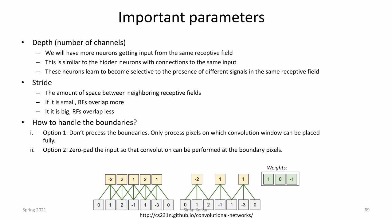
Important parameters• Depth (number of channels)
– We will have more neurons getting input from the same receptive field – This is similar to the hidden neurons with connections to the same input– These neurons learn to become selective to the presence of different signals in the same receptive field
• Stride– The amount of space between neighboring receptive fields– If it is small, RFs overlap more– It it is big, RFs overlap less
• How to handle the boundaries?i. Option 1: Don’t process the boundaries. Only process pixels on which convolution window can be placed
fully.ii. Option 2: Zero-pad the input so that convolution can be performed at the boundary pixels.
Weights:
http://cs231n.github.io/convolutional-networks/Spring 2021 Sinan Kalkan 69

Padding illustration
• Only convolution layers are shown.
• Top: no padding èlayers shrink in size.
• Bottom: zero padding è layers keep their size fixed.
Figure: Goodfellow et al., “Deep Learning”, MIT Press, 2016.Spring 2021 Sinan Kalkan 70

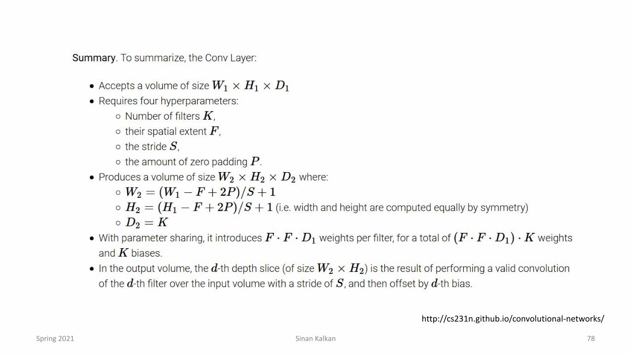
Size of the next layer• Along a dimension:
– 𝑊: Size of the input– 𝐹: Size of the receptive field– 𝑆: Stride– 𝑃: Amount of zero-padding
• Then: the number of neurons as the output of a convolution layer:𝑊 − 𝐹 + 2𝑃
𝑆+ 1
• If this number is not an integer, your strides are incorrect and your neurons cannot tile nicely to cover the input volume
http://cs231n.github.io/convolutional-networks/Zero padding
Weights:
Spring 2021 Sinan Kalkan 71

Size of the next layer
• Arranging these hyperparameters can be problematic• Example:• If W=10, P=0, and F=3, then
𝑊 − 𝐹 + 2𝑃𝑆
+ 1 =10 − 3 + 0
𝑆+ 1 =
7𝑆+ 1
i.e., 𝑆 cannot be an integer other than 1 or 7.
• Zero-padding is your friend here.
Spring 2021 Sinan Kalkan 72

Real example – AlexNet (Krizhevsky et al., 2012)
• Image size: 227×227×3
• W=227, F=11, S=4, P=0 è RRSTUUV
+ 1 = 55
(55 => the width of the convolution layer)• Convolution layer: 55×55×96 neurons
(96: the depth, the number of channels)• Therefore, the first layer has 55×55×96 = 290,400 neurons
– Each has 11×11×3 receptive field è 363 weights and 1 bias– Then, 290,400×364 = 105,705,600 parameters just for the first convolution layer (if there were
no weight sharing)– With weight sharing: 96 x 364 = 34,944
Spring 2021 Sinan Kalkan 73

• However, we can share the parameters– For each channel (slice of depth), have the same set of weights– If 96 channels, this means 96 different set of weights– Then, 96×364 = 34,944 parameters – 364 weights shared by 55×55 neurons in each channel
Real example –AlexNet (Krizhevsky et al., 2012)
http://cs231n.github.io/convolutional-networks/Spring 2021 Sinan Kalkan 74

More on connectivity
Small RF & Stacking• E.g., 3 CONV layers of 3x3 RFs• Pros:
– Same extent for these example figures– With non-linearity added with 2nd and 3rd
layers è More expressive! More representational capacity!
– Less parameters: 3 x [(3 x 3 x C) x C] = 27CxC
• Cons?
Large RF & Single Layer• 7x7 RFs of single CONV layer• Cons:
– Linear operation in one layer– More parameters: (7x7xC)xC = 49CxC
• Pros?
So, we prefer a stack of small filter sizes against big oneshttp://cs231n.github.io/convolutional-networks/Spring 2021 Sinan Kalkan 75

Implementation Details: NumPy example
• Suppose input is volume is X of shape (11,11,4)• Depth slice at depth d (i.e., channel d): X[:,:,d]• Depth column at position (x,y): X[x,y,:]• F: 5, P:0 (no padding), S=2
– Output volume (V) width, height = (11-5+0)/2+1 = 4• Example computation for some neurons in first channel:
• Note that this is just along one dimension http://cs231n.github.io/convolutional-networks/
Spring 2021 Sinan Kalkan 76

• A second activation map (channel):
Implementation Details: NumPy example
http://cs231n.github.io/convolutional-networks/Spring 2021 Sinan Kalkan 77
http://cs231n.github.io/convolutional-networks/
Spring 2021 Sinan Kalkan 78