ceng 5604 - ndl.ethernet.edu.et
TRANSCRIPT
i
CENG 5604 Hydropower Development
Lecture note
© March 2020
ii
Contents
Chapter 1 Introduction ................................................................................................................................. 1
1.1. Definition: .......................................................................................................................................... 1
1.2. History of Water Power ..................................................................................................................... 1
Water Wheels ........................................................................................................................................... 1
Pitch-back .............................................................................................................................................. 2
Over-shot .............................................................................................................................................. 2
Breast-shot ............................................................................................................................................ 2
Under-shot ............................................................................................................................................ 2
High-Speed Commercial Hydraulic Turbines ........................................................................................ 3
1.3. Types of developments ...................................................................................................................... 3
Operational features ............................................................................................................................. 4
Basis of operation ................................................................................................................................. 5
Purpose ................................................................................................................................................. 5
Basis of uses .......................................................................................................................................... 5
Hydraulic feature .................................................................................................................................. 6
Plant capacity and head ........................................................................................................................ 7
1.4. Hydropower Development Cycles .................................................................................................... 7
Reconnaissance studies ........................................................................................................................ 8
Pre-feasibility study (Preliminary Design) ............................................................................................. 9
Feasibility study................................................................................................................................... 10
Implementation Phase ........................................................................................................................ 11
1.5. Hydropower in Ethiopia ................................................................................................................... 12
Energy Policy of Ethiopia ..................................................................................................................... 14
Problems related to power production in Ethiopia ............................................................................ 15
Chapter 2: Hydraulics and Hydrology of Hydropower ................................................................................ 16
2.1. Hydraulic theory .............................................................................................................................. 16
2.2. Hydrology of hydropower ................................................................................................................ 18
Flow duration analysis ........................................................................................................................ 18
Discharge capacity of a plant .............................................................................................................. 21
Water Power Potential ........................................................................................................................ 21
iii
Other hydrologic considerations ......................................................................................................... 22
2.3. Energy and power analysis using FDC ............................................................................................ 23
Power duration curve .......................................................................................................................... 23
Load terminologies ............................................................................................................................. 28
Load Duration Curve .......................................................................................................................... 31
Chapter 3: Turbine selection and capacity determination ......................................................................... 41
3.1. Turbine types ................................................................................................................................... 41
Turbine types: Reaction ...................................................................................................................... 42
Turbine types: Impulse (or Velocity Turbines) ................................................................................... 45
3.2. Limits of use of turbine types .......................................................................................................... 48
3.3. Turbine selection criteria ................................................................................................................. 49
Rotational speed .................................................................................................................................. 49
Specific Speed ..................................................................................................................................... 50
Maximum Efficiency .......................................................................................................................... 52
3.4. Determination of number of units .................................................................................................... 53
3.5. Power House .................................................................................................................................... 55
Substructure ........................................................................................................................................ 56
Intermediate structure ......................................................................................................................... 56
Superstructure: .................................................................................................................................... 57
Power House Dimensions ................................................................................................................... 57
Underground power house .................................................................................................................. 57
Chapter 4: Water Passages ......................................................................................................................... 58
4.1. Power Canal/tunnel .......................................................................................................................... 58
Head Race: .......................................................................................................................................... 58
Tunnels ................................................................................................................................................ 62
4.2. Forebay ............................................................................................................................................ 65
4.3. Penstock ........................................................................................................................................... 66
Safe Penstock Thickness ..................................................................................................................... 67
Size Selection of Penstocks................................................................................................................. 67
Optimization of Penstock Diameter .................................................................................................... 68
Anchor blocks ..................................................................................................................................... 68
Number of penstocks .......................................................................................................................... 69

iv
4.4. Spiral casing ..................................................................................................................................... 69
4.5. Draft tubes ........................................................................................................................................ 72
Types of draft tubes ............................................................................................................................ 72
Turbine Setting .................................................................................................................................... 73
Draft tube and turbine setting.............................................................................................................. 74
Cavitation and turbine setting ............................................................................................................. 77
Chapter 5 Pressure Control and Speed Regulation..................................................................................... 79
5.1. Water hammer theory and analysis................................................................................................. 79
Elastic Water column (EWC) theory .................................................................................................... 81
Rigid water column (RWC) theory ...................................................................................................... 85
5.2. Pressure control systems ................................................................................................................. 86
Surge Tanks ......................................................................................................................................... 86
5.3. Speed terminology ........................................................................................................................... 90
5.4. Speed control and governors ........................................................................................................... 91
Exercises ...................................................................................................................................................... 92
Sample Exam ............................................................................................................................................... 97

1
Chapter 1 Introduction Contents
1. Definition
2. History of water power
3. Types of Developments:
Classification of hydro-electric
power plants
4. Hydropower development cycles
5. Hydropower in Ethiopia: Status,
Potential and Prospects
1.1. Definition:
Hydropower engineering refers to the technology involved in converting the potential energy
and kinetic energy of water into more easily used electrical energy.
The prime mover in the case of hydropower is a water wheel or hydraulic turbine which
transforms the energy of the water into mechanical energy.
Thought question: What are the Sources of water power?
1.2. History of Water Power
• Greek poet Antipater (400 B.C.) refers to energy of falling water
• ~200 B.C., Egyptians were grinding grain with horizontal water mills
• By the First Century, the wheels were turned to operate vertically (horizontal axis) at
much better efficiency
• About 1800, water mills were common in Europe
• In 1820s, Benoit Furneyron invented the turbine
• First electric power of 12 kW on Fox River, Appleton Wisconsin, 1882
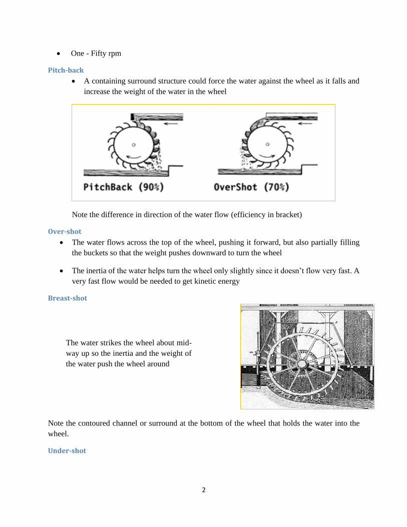
Water Wheels
Types of water wheels are based upon where the water strikes it
• Pitch-back – water drops from top and is deflected backwards to fall back towards the
dam/river
• Over-shot – shoots over the top onto the wheel; the usual kind
• Breast-shot – strikes about 50% to 80% of height of the near side of the wheel
• Under-shot – pushes underneath and need not be more than immersed in a stream
Waterwheels turn slowly compared with turbines
2
• One - Fifty rpm
Pitch-back
• A containing surround structure could force the water against the wheel as it falls and
increase the weight of the water in the wheel
Note the difference in direction of the water flow (efficiency in bracket)
Over-shot
• The water flows across the top of the wheel, pushing it forward, but also partially filling
the buckets so that the weight pushes downward to turn the wheel
• The inertia of the water helps turn the wheel only slightly since it doesn’t flow very fast. A
very fast flow would be needed to get kinetic energy
Breast-shot
The water strikes the wheel about mid-
way up so the inertia and the weight of
the water push the wheel around
Note the contoured channel or surround at the bottom of the wheel that holds the water into the
wheel.
Under-shot

3
• The undershot wheel is simply placed in
a stream with the bottom of the wheel
pushed by the current
• Works well where there is little depth and
no head
• Inefficient, but works where others won’t
• Can be on a small boat anchored in a
stream
High-Speed Commercial Hydraulic Turbines
The turbine is made to convert hydraulic
energy (potential and kinetic) into rotational
mechanical energy on the turbine shaft.
The flow discharge is controlled by an
aperture mechanism just in front of the
turbine runner.
The rotating part of the turbine or water
wheel is often referred to as the runner.
The shaft is directly connected to an electric
generator that further converts the
mechanical energy into electric energy.
The figure shows the Major Parts of a
Turbine
1.3. Types of developments
In studying the subject of hydropower engineering, it is important to understand the different
types of development. The following classification systems are commonly used:
• Operational feature (Regulation of
water flow)
• Basis of operation
• Purpose of development
• Uses to meet the demand for electrical
power
• Hydraulic feature
• Plant capacity
• Operational head
4
Operational features
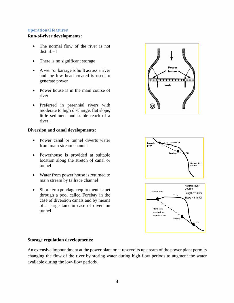
Run-of-river developments:
• The normal flow of the river is not
disturbed
• There is no significant storage
• A weir or barrage is built across a river
and the low head created is used to
generate power
• Power house is in the main course of
river
• Preferred in perennial rivers with
moderate to high discharge, flat slope,
little sediment and stable reach of a
river.
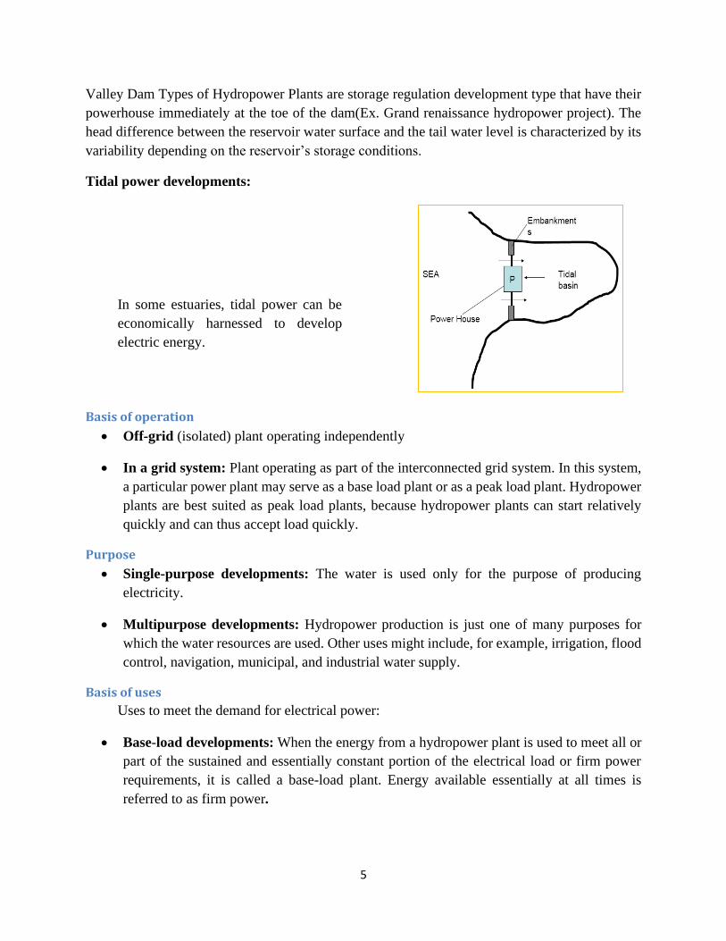
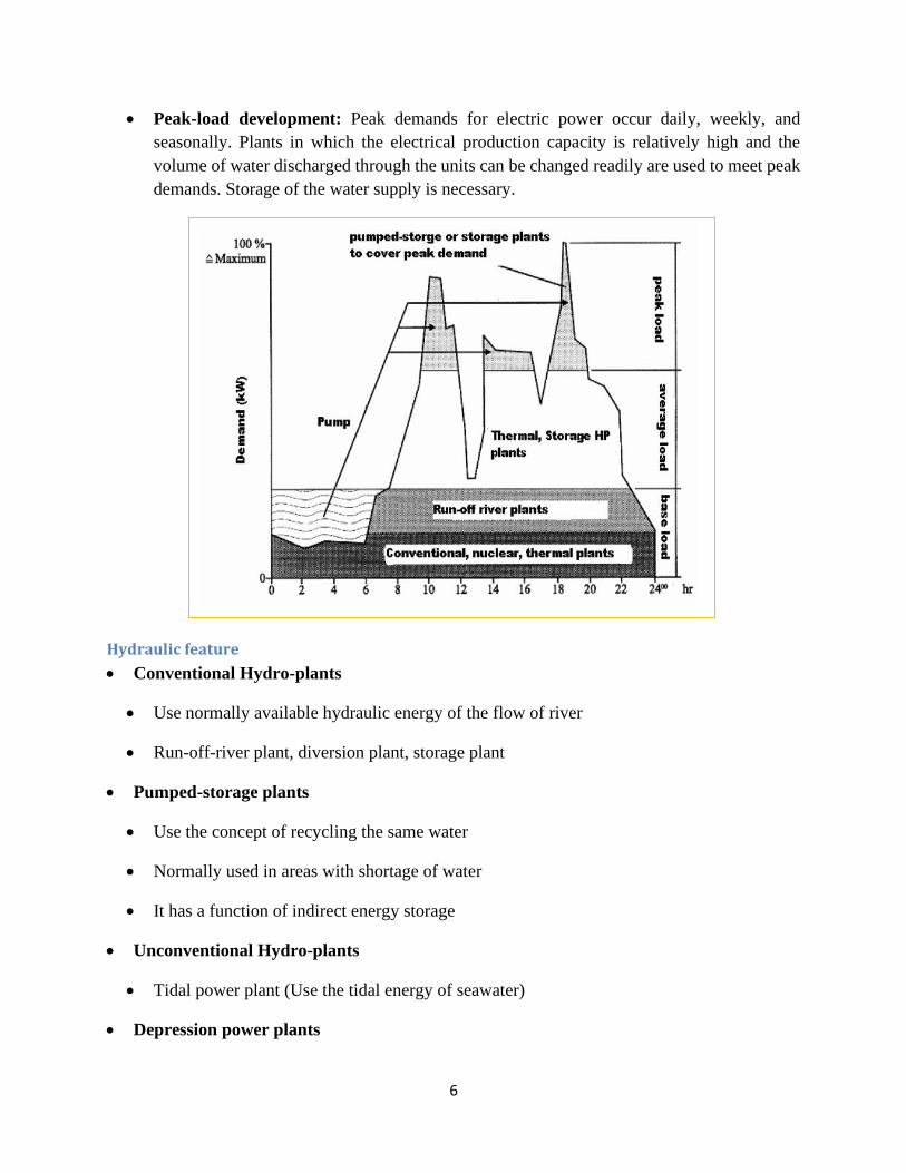
Diversion and canal developments:
• Power canal or tunnel diverts water
from main stream channel
• Powerhouse is provided at suitable
location along the stretch of canal or
tunnel
• Water from power house is returned to
main stream by tailrace channel
• Short term pondage requirement is met
through a pool called Forebay in the
case of diversion canals and by means
of a surge tank in case of diversion
tunnel
Storage regulation developments:
An extensive impoundment at the power plant or at reservoirs upstream of the power plant permits
changing the flow of the river by storing water during high-flow periods to augment the water
available during the low-flow periods.
5
Valley Dam Types of Hydropower Plants are storage regulation development type that have their
powerhouse immediately at the toe of the dam(Ex. Grand renaissance hydropower project). The
head difference between the reservoir water surface and the tail water level is characterized by its
variability depending on the reservoir’s storage conditions.
Tidal power developments:
In some estuaries, tidal power can be
economically harnessed to develop
electric energy.
Basis of operation
• Off-grid (isolated) plant operating independently
• In a grid system: Plant operating as part of the interconnected grid system. In this system,
a particular power plant may serve as a base load plant or as a peak load plant. Hydropower
plants are best suited as peak load plants, because hydropower plants can start relatively
quickly and can thus accept load quickly.
Purpose
• Single-purpose developments: The water is used only for the purpose of producing
electricity.
• Multipurpose developments: Hydropower production is just one of many purposes for
which the water resources are used. Other uses might include, for example, irrigation, flood
control, navigation, municipal, and industrial water supply.
Basis of uses
Uses to meet the demand for electrical power:
• Base-load developments: When the energy from a hydropower plant is used to meet all or
part of the sustained and essentially constant portion of the electrical load or firm power
requirements, it is called a base-load plant. Energy available essentially at all times is
referred to as firm power.
6
• Peak-load development: Peak demands for electric power occur daily, weekly, and
seasonally. Plants in which the electrical production capacity is relatively high and the
volume of water discharged through the units can be changed readily are used to meet peak
demands. Storage of the water supply is necessary.
Hydraulic feature
• Conventional Hydro-plants
• Use normally available hydraulic energy of the flow of river
• Run-off-river plant, diversion plant, storage plant
• Pumped-storage plants
• Use the concept of recycling the same water
• Normally used in areas with shortage of water
• It has a function of indirect energy storage
• Unconventional Hydro-plants
• Tidal power plant (Use the tidal energy of seawater)
• Depression power plants

7
• Energy generated by diverting water into a low lying depression
• Tailwater to be absorbed by evaporation
Plant capacity and head
• Plant capacity: Usually this type of classification is arbitrary: for example:
• Pico Hydro < 500 W
• Micro hydro < 100 kW
• Mini hydro < 1000 kW
• Small to Medium < 60 MW
• Large Hydro > 60 MW
• Classification based on head too arbitrary:
• Low head plants < 15 m
• Medium head plants 15 – 50 m
• High head plants 50-250 m
• Very high head plants > 250 m
1.4. Hydropower Development Cycles
Hydro power development involves a long process of assessing technical, commercial,
environmental and social aspects, including understanding risks and opportunities for sustainable
outcomes
• The studies to be carried out are:
• Resources studies
• Preparation/updating of resources inventories
• Preparation/updating of resources rankings
• Site specific studies
• Preliminary/reconnaissance studies
• Pre-feasibility studies
• Feasibility studies
• The main purpose of resource inventory investigation is to identify register and catalogue the
hydropower resource existing in a river basin; areas; districts and provinces.
• Flow data and data on topography is sufficient to establish the production and generating
capability of a site.

8
• The identified project sites are ranked according to size, cost, electric demand, etc.
• Preparation of resources inventories and their updating is a continuous process and should not
be stopped at any time.
Reconnaissance studies
• The details and data requirements of these studies are regional in nature.
• Accuracy of these data as a requirement is less.
• Carried out for specific purpose such as: to establish the available potential in a district.
• They are concerned with project selection from inventories of resources.
The main objectives may be such as:
• Assessment of demand or define electric power need
• Selection of candidate projects from the resources inventories which will meet the electric
power demand
• Investigation of candidate projects and project alternatives to the best technical level
• Technical ranking of candidate projects should be prepared and well recorded
• Selection of a suitable project from the list of investigated candidate projects.
• Estimation of preliminary cost and implementation schedule.
Main activities to be done in this stage:
• Data collection
• Office studies
• Field work and final reconnaissance report
Data Collection:
• Infrastructure information
• Power market and demand forecast
• Hydrology
• Topography
• Geology and geo technical
engineering
• Environmental studies
• Socio-economic set up
Office studies:

9
• Power demand forecast
• Flow regulation
• Head
• Environmental constraints
Field work: the following issues should be recorded properly
• Terrain features such as location and
placement of structures
• Infrastructures such as access to the
project, transmission lines,
• Settlement and resettlement issue
• Availability of construction material
• Environmental issues such as
diversion of flow from one catchment
to the other, deforestation, etc.
• Multipurpose uses
• Diversion of flow during construction
of Headwork and/or coffer dams
• In case of reservoir and tunnel projects
special attention shall be given to the
geological and geo technical
properties.
• Appraisal of discharge available
• Study of existing and future water uses
such as drinking, irrigation, etc.
• Verification of estimated head
• Powerhouse type, location and
equipment
Report: Any reconnaissance report must conclude with a statement on the viability and
sustainability of the project under consideration. Data requirement for feasibility study should be
indicated.
Pre-feasibility study (Preliminary Design)
In this study one or more project alternatives are proposed and studied before selection. The main
purpose of pre-feasibility is to:
• Establish demand for the project
• Formulate a plan for developing this project
• Assess if the project is technically, economically and environmentally acceptable
• Make recommendation for future action
The following aspects are to be investigated during pre-feasibility study:
1. Hydrologic study:
• Source extent amount, occurrence and variability of water.

10
• Present, past and future needs of water
• Include opportunities for control and development of water.
• Quality of water in terms of its physical and chemical properties
• Sediment quality and quantity
• Existing water rights should e recognized for each and every stakeholder.
2. Power studies: this considers a balance between power supply and demand.
3. Layout Planning: a comprehensive layout plan will be prepared and should be supplemented
with sufficient number of drawings, which will be used for preparation of the bill of quantities.
4. Geology and foundation engineering
5. Seismic studies
6. Environmental studies
7. Estimation of cost
8. Economic and financial studies
9. Future investigation plan
Pre-feasibility report: A clear statement should be made in respect of technical, economical and
environmental feasibility of the project. It should give clear indication whether or not to study the
project in more detail.
Feasibility study
Feasibility studies are carried out to determine the technical, economical and environmental
viability of a project. This phase of investigation consists of a detailed study which is directed
towards the ultimate permission, financing, final design and construction of the project under
investigation.
The main part of feasibility studies include:
1. Data Collection:
• Socioeconomic
data
• Population
• Income distribution
• Power market
• Tariffs
• Hydrology
• Topography
• Geology
• Seismic
• Environment
• Meteorology
• Infrastructure
2. Project parameter estimation
• Power and energy estimation • Power system studies

11
• Water resources studies
• Geology and foundation conditions
• Seismic studies
• Construction materials
• Existing infrastructure
3. Layout Optimization
• Project layout
• Sediment and control measures
• Number and size of units
• Auxiliary equipment
• Transmission planning
4. Environmental studies
• Assessment of environmental disturbance and their mitigation measures
5. Engineering design:
• Intake structure and sediment
excluder
• Headrace and tailrace
• Powerhouse
• Dimensioning and preparation of
specification for hydro turbine and
electromechanical equipment
• Construction facilities
6. Estimation of project cost
• Project cost
• Operation, maintenance and
replacement
• Environmental cost
• Construction planning and budgeting
• Contingencies and other costs
7. Economical and financial analysis
8. Future steps to be taken for the project implementation
Feasibility report: A clear statement should be made in respect of technical, economical and
environmental feasibility of a project. It should give clear indication whether or not to design and
implement the project.
Implementation Phase
Project implementation is a multidisciplinary job which includes:
• Approval and appropriation of funds
• Pre-qualification and hiring of
consultants
• Detailed design
• Preparation of tender/contract documents

12
• Pre-qualification of contractors
• Preparation of construction design and
engineering design
• Preparation of operation manual
• Construction supervision
• Construction of civil works
• Supply and erection of equipment
• Testing, commissioning and commercial
operation
• Preparation of completion report
1.5. Hydropower in Ethiopia
Presently there are two different power supply systems,
• The Interconnected System (ICS), which is mainly supplied from hydropower plants,
• The Self-Contained System (SCS), which consists of mini hydropower plants and a number
of isolated diesels generating units that are widely spread over the country.
• The ICS has a total installed generation capacity of about 3326.1 MW.
Storage regulated hydropower development status in Ethiopia (Source EEPCO, MoWIE, 2017).
1. Operational
No. Name River Basin Region UTME UTMN Installed
Capacity (MW)
1 Amerti Neshe Abay Oromia 309105.2 1078089.9 97
2 Fincha Abay Oromia 316215 1058323 134
3 Gibe-III O. Gibe Oromia/SNNR 312200 757200 1870
4 Gilgel Gibe I O. Gibe Oromia 319025.8 870669.51 183.9
5 Koka Awash Oromia 518144.6 936460.7 43.2
6 Melkawakena W. Shebele Oromia 547907.5 792277.08 153
7 Tana Beles Abay Amhara 284013.4 1313351.9 460
8 Tekeze-1 Tekaze Tigray/Amhara 472125 1475533 300
9 Tis-Abay-I Abay Amhara 338393.1 1272689 12
10 Tis-Abay-II Abay Amhara 345289 1270370 73
Total Functional 3326.1
2. Under Construction
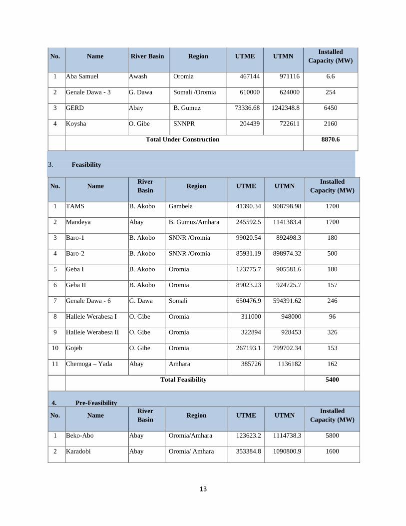
13
No. Name River Basin Region UTME UTMN Installed
Capacity (MW)
1 Aba Samuel Awash Oromia 467144 971116 6.6
2 Genale Dawa - 3 G. Dawa Somali /Oromia 610000 624000 254
3 GERD Abay B. Gumuz 73336.68 1242348.8 6450
4 Koysha O. Gibe SNNPR 204439 722611 2160
Total Under Construction 8870.6
3. Feasibility
No. Name River
Basin Region UTME UTMN
Installed
Capacity (MW)
1 TAMS B. Akobo Gambela 41390.34 908798.98 1700
2 Mandeya Abay B. Gumuz/Amhara 245592.5 1141383.4 1700
3 Baro-1 B. Akobo SNNR /Oromia 99020.54 892498.3 180
4 Baro-2 B. Akobo SNNR /Oromia 85931.19 898974.32 500
5 Geba I B. Akobo Oromia 123775.7 905581.6 180
6 Geba II B. Akobo Oromia 89023.23 924725.7 157
7 Genale Dawa - 6 G. Dawa Somali 650476.9 594391.62 246
8 Hallele Werabesa I O. Gibe Oromia 311000 948000 96
9 Hallele Werabesa II O. Gibe Oromia 322894 928453 326
10 Gojeb O. Gibe Oromia 267193.1 799702.34 153
11 Chemoga – Yada Abay Amhara 385726 1136182 162
Total Feasibility 5400
4. Pre-Feasibility
No. Name River
Basin Region UTME UTMN
Installed
Capacity (MW)
1 Beko-Abo Abay Oromia/Amhara 123623.2 1114738.3 5800
2 Karadobi Abay Oromia/ Amhara 353384.8 1090800.9 1600

14
No. Name River
Basin Region UTME UTMN
Installed
Capacity (MW)
3 Wabishebele (WS)-18 W. Shebele Somali/ Oromia 844070.2 824634.32 87.5
4 Mabil Abay Oromia/Amhara 315603 1109013 1650
5 Beshilo Abay Amhara 445441 1213597 700
6 Tekeze -2 Tekeze Tigray 381997.8 1533150.2 450
7 Gibe-4 O. Gibe SNNPR 230736.2 728351.61 1472
8 Gibe 5 O. Gibe SNNPR 173976.9 697557.96 436
9 Upper Dabus Abay B. Gumuz/Oromia 50206.29 1101645.3 326.28
10 Lower Dedessa Abay Oromia 167256.2 1049164.6 301
11 Lower Dabus Abay B. Gumuz/Oromia 50206.29 1101645.3 326.28
12 Birbir A B. Akobo Oromia 80961.22 946311.39 97.4
13 Birbir-R B. Akobo Oromia 79927.78 942897.9 467
Total Pre-Feasibility 13713.46
Energy Policy of Ethiopia
Ethiopia’s national energy policy identifies hydropower as the backbone of its sectoral
development strategy. In 2005, the Government of Ethiopia released an aggressive, 25-year
national energy master plan. The plan is updated annually and allows EEPCO great flexibility to
easily integrate new projects. Besides its 25-year master plan, EEPCO is also undertaking an
aggressive five-year plan called the Universal Rural Electrification Access Program (UREAP) to
expand the domestic grid. The UREAP’s goal is to increase access to electricity to 50% of the
population. The Energy policy that corresponds to demand and consumption envisages to meet the
following broad objectives:
• Giving high priority to Renewable Energy Development and follows climate resilient
green economy strategy
• Considers Hydropower as the backbone of the country’s energy generation and maximize
its utilization;
• Enhancing regional and global cooperation in the energy sector to ensure exchange of
know-how, information and transfer of technologies
• Strengthening cross boarder energy trade.
• Increasing access to affordable and adequate modern energy.

15
• Promoting efficient, clean, and appropriate energy technologies and conservation
measure.
• Improving the energy efficiency of systems and operations.
Problems related to power production in Ethiopia
• Lowest income (550 USD, in 2014?)
• High rate of population growth (2.8%)
• Scattered settlement pattern (>80% rural, 63 person/km2)
• High investment cost (800 to 3000 USD/KW)
o Too low domestic investors ability
o Low credit availability (most of the project construction materials could easily
be obtained in Ethiopia)
• Higher cost and time-consuming study and design phase.
• Higher risk (commercial, political, construction and hydrological risks)
• Lack of integrated water resources management
• Low domestic capacity building… etc.
16
Chapter 2: Hydraulics and Hydrology of Hydropower Contents
1. Hydraulic Theory
2. Hydrologic analysis for hydropower
1. Flow Duration Analysis
2. Other Hydrologic
Considerations
3. Energy and Power Analysis Using
Flow Duration Approach
1. Power duration curve
2. Load terminologies
3. Load duration curve
2.1. Hydraulic theory
Energy-work approach:
• Work (W) = Force x Distance in the direction of force
• Work = weight of water x the distance it falls ghVW ww=
Where: ρw is density of water; g- acceleration due to gravity; Vw- volume of water falling; h- the
vertical distance the water falls.
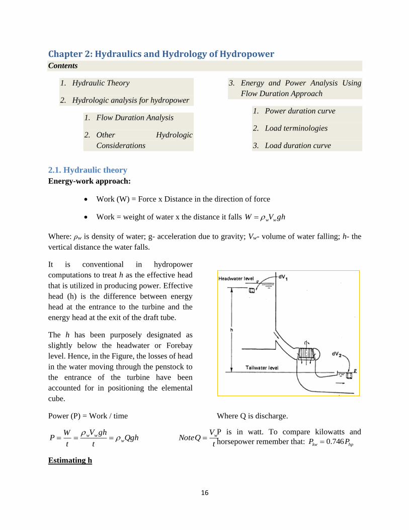
It is conventional in hydropower
computations to treat h as the effective head
that is utilized in producing power. Effective
head (h) is the difference between energy
head at the entrance to the turbine and the
energy head at the exit of the draft tube.
The h has been purposely designated as
slightly below the headwater or Forebay
level. Hence, in the Figure, the losses of head
in the water moving through the penstock to
the entrance of the turbine have been
accounted for in positioning the elemental
cube.
Power (P) = Work / time
t
VQNoteQgh
t
ghV
t
WP w
w
ww ====
Where Q is discharge.
P is in watt. To compare kilowatts and
horsepower remember that: hpkw PP 746.0=
Estimating h
17
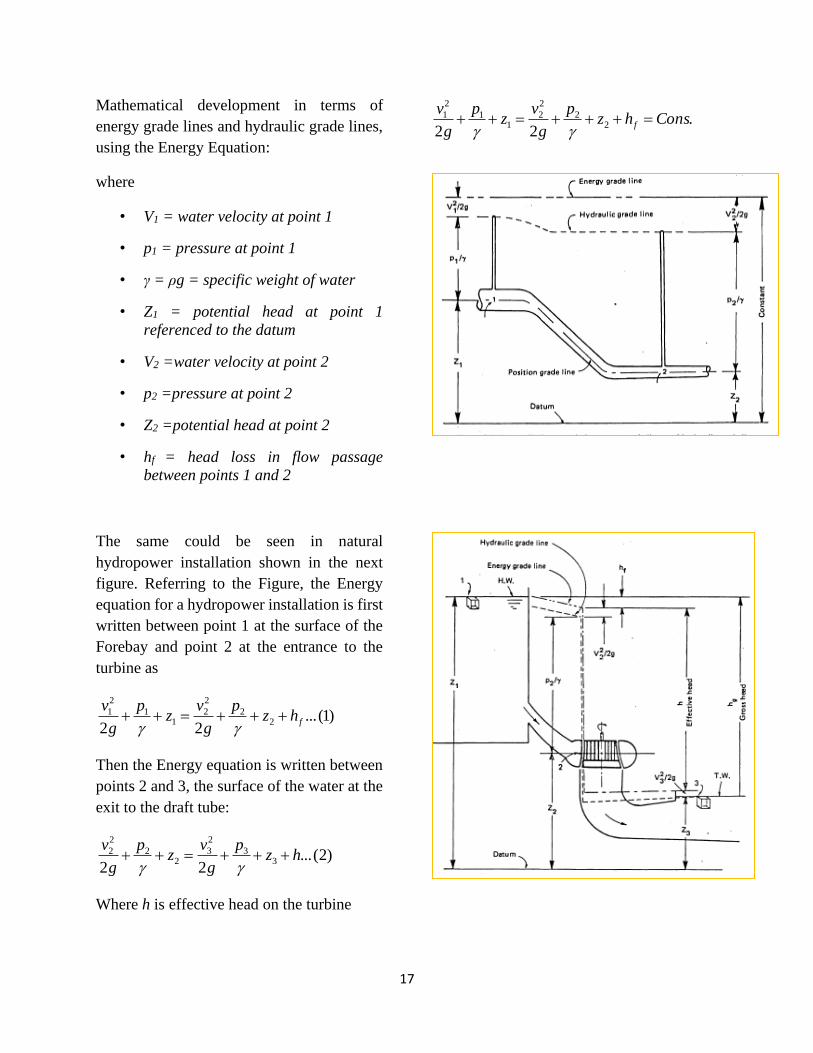
Mathematical development in terms of
energy grade lines and hydraulic grade lines,
using the Energy Equation:
.22
22
2
21
1
2
1 Conshzp
g
vz
p
g
vf =+++=++
where
• V1 = water velocity at point 1
• p1 = pressure at point 1
• γ = ρg = specific weight of water
• Z1 = potential head at point 1
referenced to the datum
• V2 =water velocity at point 2
• p2 =pressure at point 2
• Z2 =potential head at point 2
• hf = head loss in flow passage
between points 1 and 2
The same could be seen in natural
hydropower installation shown in the next
figure. Referring to the Figure, the Energy
equation for a hydropower installation is first
written between point 1 at the surface of the
Forebay and point 2 at the entrance to the
turbine as
)1(...22
22
2
21
1
2
1fhz
p
g
vz
p
g
v+++=++
Then the Energy equation is written between
points 2 and 3, the surface of the water at the
exit to the draft tube:
)2(...22
33
2
32
2
2
2 hzp
g
vz
p
g
v+++=++
Where h is effective head on the turbine
18
Recognizing that for practical purposes v1, p1, and p3 are equal to zero, then solving for p2/γ in Eq.
1, the result is:
)3(...2
2
2
21
2fhz
g
vz
p−−−=
)4...(2
22222
2
331
3
2
322
2
21
2
23
2
32
2
2
2
g
vhzzh
zg
vzhz
g
vz
g
vz
g
vz
p
g
vh
f
f
−−−=
−−+
−−−+=−−++=
Because the Energy equation defines terms in units of Kilogram –meter per Kilogram of water
flowing through the system, it should be recognized that the Kilograms of water flowing through
the turbine per unit of time by definition is ρgq.
Now recognizing that energy per unit of time is power, it is simple to calculate power by
multiplying Eq. (4) by ρgq or γq to obtain the theoretical power delivered by the water to the
turbine as γqh which is the theoretical power
2.2. Hydrology of hydropower
• Hydrology is the study of the occurrence, movement and distribution of water on, above,
and within the earth's surface.
• Parameters necessary in making hydropower studies are water discharge (Q) and hydraulic
head (h). The measurement and analyses of these parameters are primarily hydrologic
problems.
• Determination of the head for a proposed hydropower plant is a surveying problem that
identifies elevations of water surfaces as they are expected to exist during operation of the
hydropower plant.
• In some reconnaissance studies, good contour maps may be sufficient to determine the value
for the hydraulic head.
• Because the headwater elevation and tailwater elevations of the impoundment can vary with
stream flow, it is frequently necessary to develop headwater and tailwater curves that show
variation with time, river discharge, or operational features of the hydropower project.
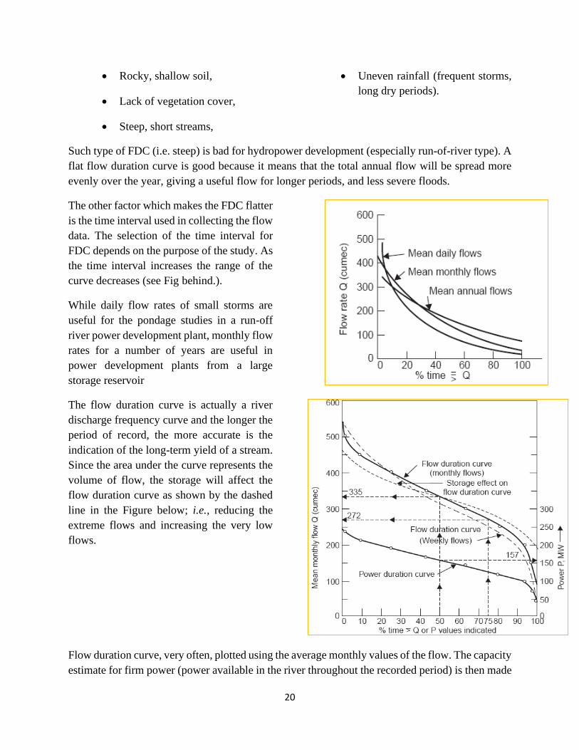
Flow duration analysis
Flow Duration Curves: is a plot of flow
versus the percent of time a particular flow
can be expected to be equaled or exceeded.
A flow duration curve merely reorders the
flows in order of magnitude instead of the
true time ordering of flows in a flow versus
time plot.
19
• Two methods
o The rank ordered technique and
o The class-interval technique.
The rank-ordered technique
Considers a total time series of flows that represent equal increments of time for each measurement
value, such as mean daily, weekly, or monthly flows, and ranks the flows according to magnitude.
The rank-ordered values are assigned individual order numbers, the largest beginning with order
1. The order numbers are then divided by the total number in the record and multiplied by 100 to
obtain the percent of time that the mean flow has been equaled or exceeded during the period of
record being considered.
The flow value is then plotted versus the respective computed exceedance percentage. Naturally,
the longer the record, the more statistically valuable the information that results.
The class-interval technique
It is slightly different in that the time series of flow values are categorized into class intervals. The
classes range from the highest flow value to the lowest value in the time series. A tally is made of
the number of flows in each, and by summation the number of values greater than a given upper
limit of the class can be determined.
• The number of flows greater than the upper limit of a class interval can be divided by the
total number of flow values in the data series to obtain the exceedance percentage.
• The value of the flow for the particular upper limit of the class interval is then plotted versus
the computed exceedance percent.
Characteristics of Flow Duration Curves
The flow duration curve (FDC) shows how flow is distributed over a period (usually a year). A
steep flow duration curve implies a flashy catchment – one which is subject to extreme floods and
droughts.
Factors which cause a catchment to be flashy are:
0
20
40
60
80
100
120
140
0 20 40 60 80 100
Dis
cha
rge
in m
3/s
Exceedence in %
20
• Rocky, shallow soil,
• Lack of vegetation cover,
• Steep, short streams,
• Uneven rainfall (frequent storms,
long dry periods).
Such type of FDC (i.e. steep) is bad for hydropower development (especially run-of-river type). A
flat flow duration curve is good because it means that the total annual flow will be spread more
evenly over the year, giving a useful flow for longer periods, and less severe floods.
The other factor which makes the FDC flatter
is the time interval used in collecting the flow
data. The selection of the time interval for
FDC depends on the purpose of the study. As
the time interval increases the range of the
curve decreases (see Fig behind.).
While daily flow rates of small storms are
useful for the pondage studies in a run-off
river power development plant, monthly flow
rates for a number of years are useful in
power development plants from a large
storage reservoir
The flow duration curve is actually a river
discharge frequency curve and the longer the
period of record, the more accurate is the
indication of the long-term yield of a stream.
Since the area under the curve represents the
volume of flow, the storage will affect the
flow duration curve as shown by the dashed
line in the Figure below; i.e., reducing the
extreme flows and increasing the very low
flows.
Flow duration curve, very often, plotted using the average monthly values of the flow. The capacity
estimate for firm power (power available in the river throughout the recorded period) is then made
21
by using the entire recorded flow data and plotting in a single flow duration curve. In such a case
two different methods are in use.
(i) The total period method, and
(ii) The calendar year method.
Both methods utilize the flow data available for the entire period for which records are available.
Total period method: the entire available record is used for drawing the FDC. Thus, ten years’
record would produce 120 values of monthly average flows.
▪ These are first tabulated in the ascending order starting from the driest month in the
entire period and ending with the wettest month of the ten-year duration.
▪ The FDC would then be drawn with the help of 120 values.
Calendar year method: each year’s average monthly values are first arranged in ascending order.
▪ Then the average flow values corresponding to the driest month, second driest month,
and so on up to the wettest month are found out by taking arithmetic mean of all values
of the same rank. These average values are then used for plotting flow duration curve.
▪ Such a curve would have only twelve points.
The total period method gives more correct results than the calendar year method which
averages out extreme events.
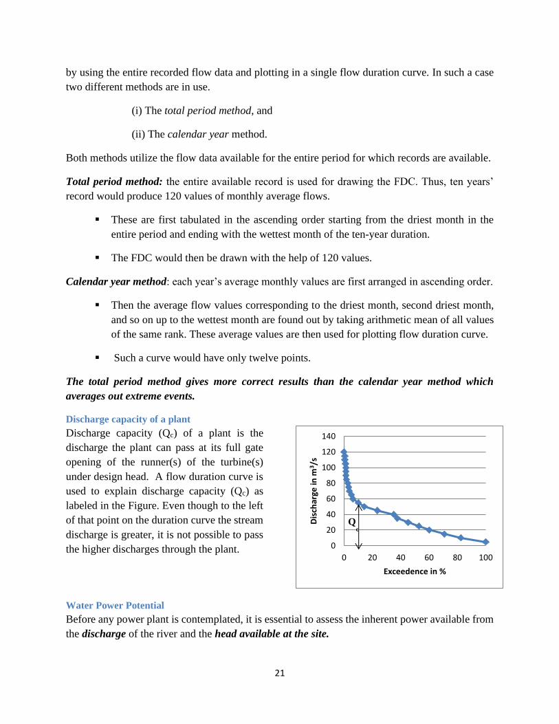
Discharge capacity of a plant
Discharge capacity (Qc) of a plant is the
discharge the plant can pass at its full gate
opening of the runner(s) of the turbine(s)
under design head. A flow duration curve is
used to explain discharge capacity (Qc) as
labeled in the Figure. Even though to the left
of that point on the duration curve the stream
discharge is greater, it is not possible to pass
the higher discharges through the plant.
Water Power Potential
Before any power plant is contemplated, it is essential to assess the inherent power available from
the discharge of the river and the head available at the site.
0
20
40
60
80
100
120
140
0 20 40 60 80 100
Dis
char
ge in
m3 /
s
Exceedence in %
Qc
22
• The gross head of any proposed scheme can be assessed by simple surveying techniques,
whereas
• Hydrological data on rainfall and runoff are essential in order to assess the quantity of
water available.
• The hydrological data necessary for potential assessment are:
▪ The daily, weekly, or monthly flow over a period of several years, to determine
the plant capacity and estimate output,
▪ Low flows, to assess the primary, firm or dependable power.
Other hydrologic considerations
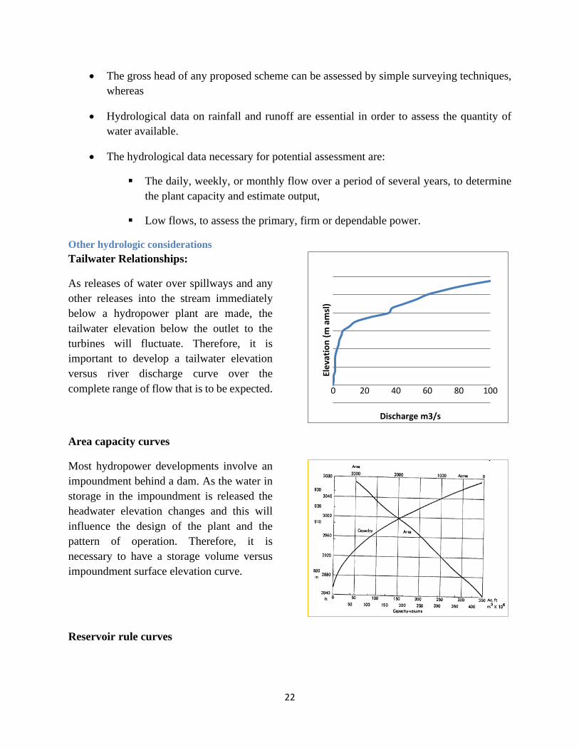
Tailwater Relationships:
As releases of water over spillways and any
other releases into the stream immediately
below a hydropower plant are made, the
tailwater elevation below the outlet to the
turbines will fluctuate. Therefore, it is
important to develop a tailwater elevation
versus river discharge curve over the
complete range of flow that is to be expected.
Area capacity curves
Most hydropower developments involve an
impoundment behind a dam. As the water in
storage in the impoundment is released the
headwater elevation changes and this will
influence the design of the plant and the
pattern of operation. Therefore, it is
necessary to have a storage volume versus
impoundment surface elevation curve.
Reservoir rule curves
0 20 40 60 80 100
Ele
vati
on
(m
am
sl)
Discharge m3/s
23
When releases from reservoirs are made, the schedule of releases is often dictated by
considerations other than just meeting the flow demands for power production. The needs for
municipal water supply, for flood control, and for downstream use dictate certain restraints. The
restraints are conventionally taken care of by developing reservoir operation rule curves that can
guide operating personnel in making necessary changes in reservoir water releases.
Evaporation Loss Evaluation: Where there is an impoundment involved in a hydropower
development there is need to assess the effect of evaporation loss from the reservoir surface.
Spillway Design Flood Analysis: Many hydropower developments require a dam or a diversion
that blocks the normal river flow. This then requires that provisions be made for passing flood
flows. Spillway design flood analysis treats a unique type of hydrology that concerns the
occurrence of rare events of extreme flooding. It is customary on larger dams and dams where
failure might cause a major disaster to design the spillway to pass the probable maximum flood.
For small dams, spillways are designed to pass a standard project flood.
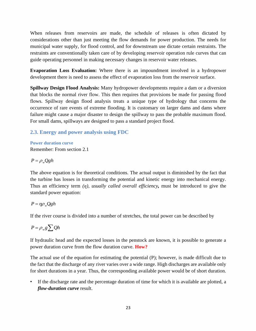
2.3. Energy and power analysis using FDC
Power duration curve
Remember: From section 2.1
QghP w=
The above equation is for theoretical conditions. The actual output is diminished by the fact that
the turbine has losses in transforming the potential and kinetic energy into mechanical energy.
Thus an efficiency term (ɳ), usually called overall efficiency, must be introduced to give the
standard power equation:
QghP w=
If the river course is divided into a number of stretches, the total power can be described by
= QhgP w
If hydraulic head and the expected losses in the penstock are known, it is possible to generate a
power duration curve from the flow duration curve. How?
The actual use of the equation for estimating the potential (P); however, is made difficult due to
the fact that the discharge of any river varies over a wide range. High discharges are available only
for short durations in a year. Thus, the corresponding available power would be of short duration.
• If the discharge rate and the percentage duration of time for which it is available are plotted, a
flow-duration curve result.
24
• Power duration curve can also be plotted since power is directly proportional to the discharge
and available head.
Discharge/Power duration curve indicates discharge or power available in the stream for the given
percentage of time. The available power from a run-of-river plant could be represented by a power
duration curve exactly on lines analogous to a FDC.
Generally, the head variation in a run-of-river plant is considerably less than the discharge
variation. If the head is presumed to be constant at an average value, power duration curve would
exactly correspond to FDC. This is very often the procedure in elementary rough calculations. If,
however, a precise power duration curve is desired, then the head corresponding to any discharge
is required to be known.
Some common terminologies
▪ Minimum potential (P100) power computed from the minimum flow available for 100 %
of the time (365 days or 8760 hours).
▪ Small potential (P95) power computed from the flow available for 95 % of time (flow
available for 8322 hours).
▪ Average potential power (P50) computed from the flow available for 50% of the time (flow
available for 6 months or 4380 hours).
▪ Mean potential power (Pm) computed from the average of mean yearly flows for a period
of 10 to 30 years, which is equal to the area of the flow-duration curve corresponding to
this mean year. This is known as ‘Gross river power potential’.
▪ It would be more significant to find out the technically available power from the potential
power; According to Mosonyi, the losses subtracted from the P values present an upper
limit of utilization;
Percentage of time equaled or exceeded
0 100
Pow
er
95 50
P50
Pm P
95 P
100
25
▪ Technically available power: With conveyance efficiency of 70% and overall efficiency
of the plant as 80%, a combined multiplying factor of 0.56 should be used with the average
potential power, P50; 5056.0 PPa =
The value of net water power capable of being developed technically is also computed from the
potential water power by certain reduction factors to account for losses of head in the conveyance
and losses associated with energy conversion. This factor is usually about 0.75 or 0.80, i.e.
( ) hQtoP mnetm 0.84.7= ; Where Qm = the arithmetic mean discharge
The maximum river energy potential is given by ( )KwhPE netmnet 8760max =
Energy production for a year or a time period is the product of the power ordinate and time and is
thus the area under the power duration curve multiplied by an appropriate conversion factor.
Example 1: What is wrong with the PDC?
0
20
40
60
80
100
120
140
0 20 40 60 80 100
Dis
char
ge in
m3
/s
Exceedence in %
FDC
0
20
40
60
80
100
120
0 20 40 60 80 100
Po
we
r in
MW
Exceedence in %
Qc
26
Example 2: The following is the record of average yearly flow in a river for 15 years. If the
available head is 15 m, construct the FDC and power duration curve for the river.
Year 1956 1957 1958 1959 1960 1961 1962 1963 1964
Flow (m3/s) 905 865 1050 1105 675 715 850 775 590
Year 1965 1966 1967 1968 1969 1970
Flow (m3/s) 625 810 885 1025 1150 925
Solution: The yearly flow values are arranged in ascending order (see table below). The power
corresponding to each flow values are calculated assuming the head (=15 m) to be constant. Then,
FDC and power duration curves are plotted on the same graph.
Row1: Rank; Raw 2: Flow in ascending order (m3/s); Raw 3: Power (=9.81 QH) [kW]; and
Raw 4: Percentage of time exceeded = ( 15 +1 – n )*100/15
R1 1 2 3 4 5 6 7
R2 590 625 675 715 775 810 850
R3 86819 91969 99326 105212 114041 119192 125078
R4 100 93.4 86.7 80 73.4 66.7 60
R1 8 9 10 11 12 13 14 15
R2 865 885 905 925 1025 1050 1105 1150
R3 127285 130228 133171 136114 150829 154508 162601 169223
R4 53.4 46.7 40 33.3 26.7 20 13.3 6.7
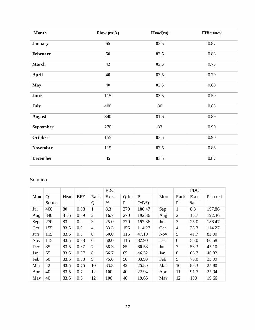
Example 3: Draw the flow and power duration curve if the discharge capacity Qc = 270 m3/s
80
100
120
140
160
180
500
600
700
800
900
1000
1100
1200
0.0 20.0 40.0 60.0 80.0 100.0
Po
we
r, k
W
Flo
w, m
3/s
% of time equalled or exceeded
Flow
27
Month Flow (m3/s) Head(m) Efficiency
January 65 83.5 0.87
February 50 83.5 0.83
March 42 83.5 0.75
April 40 83.5 0.70
May 40 83.5 0.60
June 115 83.5 0.50
July 400 80 0.88
August 340 81.6 0.89
September 270 83 0.90
October 155 83.5 0.90
November 115 83.5 0.88
December 85 83.5 0.87
Solution
FDC
PDC
Mon Q
Sorted
Head EFF Rank
Q
Exce.
%
Q for
P
P
(MW)
Mon Rank
P
Exce.
%
P sorted
Jul 400 80 0.88 1 8.3 270 186.47
Sep 1 8.3 197.86
Aug 340 81.6 0.89 2 16.7 270 192.36
Aug 2 16.7 192.36
Sep 270 83 0.9 3 25.0 270 197.86
Jul 3 25.0 186.47
Oct 155 83.5 0.9 4 33.3 155 114.27
Oct 4 33.3 114.27
Jun 115 83.5 0.5 6 50.0 115 47.10
Nov 5 41.7 82.90
Nov 115 83.5 0.88 6 50.0 115 82.90
Dec 6 50.0 60.58
Dec 85 83.5 0.87 7 58.3 85 60.58
Jun 7 58.3 47.10
Jan 65 83.5 0.87 8 66.7 65 46.32
Jan 8 66.7 46.32
Feb 50 83.5 0.83 9 75.0 50 33.99
Feb 9 75.0 33.99
Mar 42 83.5 0.75 10 83.3 42 25.80
Mar 10 83.3 25.80
Apr 40 83.5 0.7 12 100 40 22.94
Apr 11 91.7 22.94
May 40 83.5 0.6 12 100 40 19.66
May 12 100 19.66
28
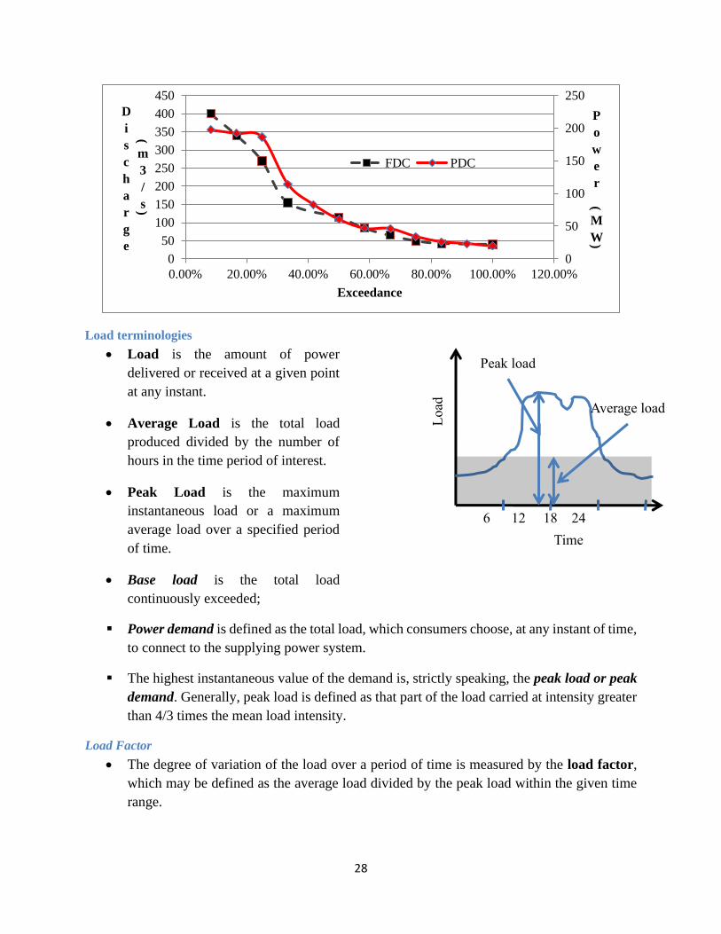
Load terminologies
• Load is the amount of power
delivered or received at a given point
at any instant.
• Average Load is the total load
produced divided by the number of
hours in the time period of interest.
• Peak Load is the maximum
instantaneous load or a maximum
average load over a specified period
of time.
• Base load is the total load
continuously exceeded;
▪ Power demand is defined as the total load, which consumers choose, at any instant of time,
to connect to the supplying power system.
▪ The highest instantaneous value of the demand is, strictly speaking, the peak load or peak
demand. Generally, peak load is defined as that part of the load carried at intensity greater
than 4/3 times the mean load intensity.
Load Factor
• The degree of variation of the load over a period of time is measured by the load factor,
which may be defined as the average load divided by the peak load within the given time
range.
0
50
100
150
200
250
0
50
100
150
200
250
300
350
400
450
0.00% 20.00% 40.00% 60.00% 80.00% 100.00% 120.00%
P
o
w
e
r
(
M
W)D
i
s
c
h
a
r
g
e
(
m
3
/
s)
Exceedance
FDC PDC
Time
Load
6 12 18 24
Average load
Peak load
29
• The load factor measures variation only and does not give any indication of the precise
shape of the load-duration curve.
• The area under the load curve represents the energy consumed in kWh; Thus, a daily load
factor may also be defined as the ratio of the actual energy consumed during 24 hours to
the peak demand assumed to continue for 24 hours.
• Load factor gives an idea of degree of utilization of capacity;
• Thus, an annual load factor of 0.4 indicates that the machines are producing only 40% of
their yearly production capacity.
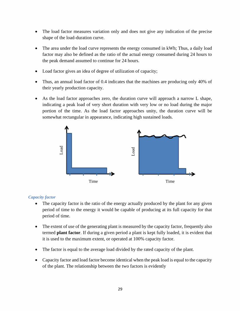
• As the load factor approaches zero, the duration curve will approach a narrow L shape,
indicating a peak load of very short duration with very low or no load during the major
portion of the time. As the load factor approaches unity, the duration curve will be
somewhat rectangular in appearance, indicating high sustained loads.
Capacity factor
• The capacity factor is the ratio of the energy actually produced by the plant for any given
period of time to the energy it would be capable of producing at its full capacity for that
period of time.
• The extent of use of the generating plant is measured by the capacity factor, frequently also
termed plant factor. If during a given period a plant is kept fully loaded, it is evident that
it is used to the maximum extent, or operated at 100% capacity factor.
• The factor is equal to the average load divided by the rated capacity of the plant.
• Capacity factor and load factor become identical when the peak load is equal to the capacity
of the plant. The relationship between the two factors is evidently
Time
Load
Time
Load
30
planttheofcapacityRated
factorLoadLoadPeakFactorCapacity
=
Plant use factor:
Capacity factor = (actual energy produced)/(energy which could have been produced had the
plant run at full rated output). Both numerator and denominator are taken over the same time.
Plant Use factor = (actual energy produced)/(energy which could have been produced had the
plant been run). Again both are taken over the same time. These are not the same because the
plant's capacity may have been reduced for many possible reasons (e.g. shortage of water) and if
it had run it would have been at below rated output. This makes the capacity factor normally a
lower number than the use factor.
periodsametheinproducedenergyMaximum
periodainusedenergyActualfactorUsePlant =
Utilization Factor
The utilization factor measures the use made of the total installed capacity of the plant. It is defined
as the ratio of the peak load and the rated capacity of the plant.
Utilization Factor: is the ratio of the quantity of water actually utilized for power production to
that available in the river. If the head is assumed to be constant, then the utilization factor would
be equal to the ratio of power utilized to that available.
The factor for a plant depends upon the type of system of which it is a part of. A low utilization
factor may mean that the plant is used only for stand-by purposes on a system comprised of several
stations or that capacity has been installed well in advance of need.
In the case of a plant in a large system, high utilization factor indicates that the plant is probably
the most efficient in the system. In the case of isolated plants a high value means the likelihood of
good design with some reserve-capacity allowance.
The value of utilization factor varies between 0.4 and 0.9 depending on the plant capacity, load
factor and storage.
Diversity factor
Diversity factor (DF) is the summation of the different types of load divided by the peak load. If
there be four different types of load L1, L2, L3 and L4 and the peak load from the combination of
these loads is LP, then the diversity factor is expressed as:
(L1 + L2 + L3 + L4)/LP
Note that the diversity factor has a value which is greater than unity. Its value could be 1 which
indicates the maximum demand of the individual sub-system occurs simultaneously.
31
For n load combination: p
ni
i
i LLDF =
=
=1
An area served by a power plant having different types of load, peaking at different times, the
installed capacity is determined by dividing the total of maximum peak load by diversity factor.
Load Duration Curve
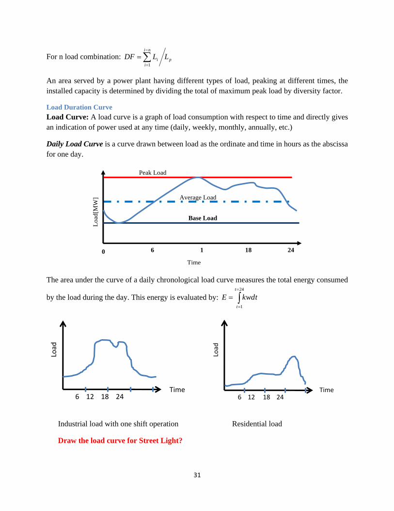
Load Curve: A load curve is a graph of load consumption with respect to time and directly gives
an indication of power used at any time (daily, weekly, monthly, annually, etc.)
Daily Load Curve is a curve drawn between load as the ordinate and time in hours as the abscissa
for one day.
The area under the curve of a daily chronological load curve measures the total energy consumed
by the load during the day. This energy is evaluated by: =
=
=
24
1
t
t
kwdtE
Industrial load with one shift operation Residential load
Draw the load curve for Street Light?
Lo
ad[M
W]
0 6 1
2
18 24
Time
Base Load
Average Load
Peak Load
Time
Load
6 12 18 24 Time
Load
6 12 18 24
32
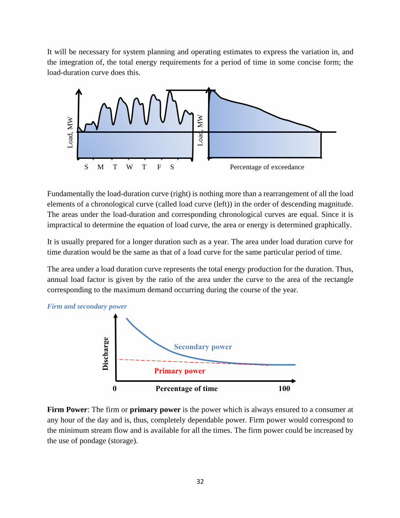
It will be necessary for system planning and operating estimates to express the variation in, and
the integration of, the total energy requirements for a period of time in some concise form; the
load-duration curve does this.
Fundamentally the load-duration curve (right) is nothing more than a rearrangement of all the load
elements of a chronological curve (called load curve (left)) in the order of descending magnitude.
The areas under the load-duration and corresponding chronological curves are equal. Since it is
impractical to determine the equation of load curve, the area or energy is determined graphically.
It is usually prepared for a longer duration such as a year. The area under load duration curve for
time duration would be the same as that of a load curve for the same particular period of time.
The area under a load duration curve represents the total energy production for the duration. Thus,
annual load factor is given by the ratio of the area under the curve to the area of the rectangle
corresponding to the maximum demand occurring during the course of the year.
Firm and secondary power
Firm Power: The firm or primary power is the power which is always ensured to a consumer at
any hour of the day and is, thus, completely dependable power. Firm power would correspond to
the minimum stream flow and is available for all the times. The firm power could be increased by
the use of pondage (storage).
Lo
ad,
MW
S M T W T F S Percentage of exceedance
Lo
ad,
MW
Percentage of time
Primary power Dis
cha
rge
0 100
Secondary power
33
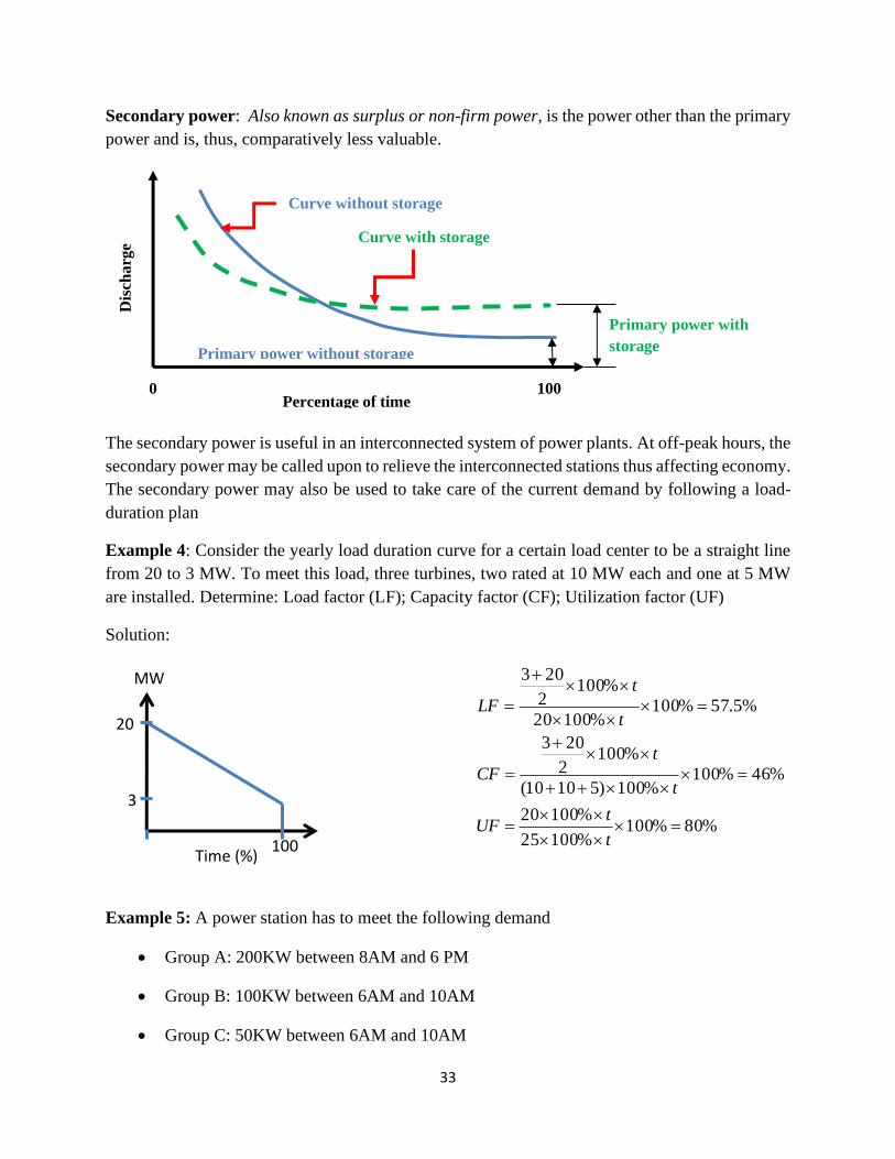
Secondary power: Also known as surplus or non-firm power, is the power other than the primary
power and is, thus, comparatively less valuable.
The secondary power is useful in an interconnected system of power plants. At off-peak hours, the
secondary power may be called upon to relieve the interconnected stations thus affecting economy.
The secondary power may also be used to take care of the current demand by following a load-
duration plan
Example 4: Consider the yearly load duration curve for a certain load center to be a straight line
from 20 to 3 MW. To meet this load, three turbines, two rated at 10 MW each and one at 5 MW
are installed. Determine: Load factor (LF); Capacity factor (CF); Utilization factor (UF)
Solution:
%80%100%10025
%10020
%46%100%100)51010(
%1002
203
%5.57%100%10020
%1002
203
=
=
=++
+
=
=
+
=
t
tUF
t
t
CF
t
t
LF
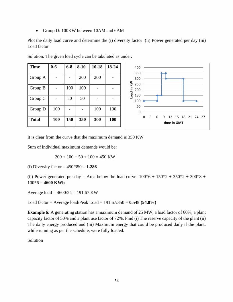
Example 5: A power station has to meet the following demand
• Group A: 200KW between 8AM and 6 PM
• Group B: 100KW between 6AM and 10AM
• Group C: 50KW between 6AM and 10AM
Percentage of time 0
Dis
ch
arg
e
100
Primary power without storage
Primary power with
storage
Curve with storage
Curve without storage
Time (%)
20
MW
3
100
34
• Group D: 100KW between 10AM and 6AM
Plot the daily load curve and determine the (i) diversity factor (ii) Power generated per day (iii)
Load factor
Solution: The given load cycle can be tabulated as under:
Time 0-6 6-8 8-10 10-18 18-24
Group A - - 200 200 -
Group B - 100 100 - -
Group C - 50 50 - -
Group D 100 - - 100 100
Total 100 150 350 300 100
It is clear from the curve that the maximum demand is 350 KW
Sum of individual maximum demands would be:
200 + 100 + 50 + 100 = 450 KW
(i) Diversity factor = 450/350 = 1.286
(ii) Power generated per day = Area below the load curve: 100*6 + 150*2 + 350*2 + 300*8 +
100*6 = 4600 KWh
Average load = 4600/24 = 191.67 KW
Load factor = Average load/Peak Load = 191.67/350 = 0.548 (54.8%)
Example 6: A generating station has a maximum demand of 25 MW, a load factor of 60%, a plant
capacity factor of 50% and a plant use factor of 72%. Find (i) The reserve capacity of the plant (ii)
The daily energy produced and (iii) Maximum energy that could be produced daily if the plant,
while running as per the schedule, were fully loaded.
Solution
0
50
100
150
200
250
300
350
400
0 3 6 9 12 15 18 21 24 27
Load
in K
W
time in GMT
35
MWDemandAverageDemandMaximum
DemandAverageFL 15256.06.0.. ====
MWdemandMaximumcapacityPlantcapacityserve
MWCapacityPlantCapacityPlant
DemandAverageFCPlant
52530Re
305.0
155.0..
=−=−=
====
Daily energy produced = Average demand * 24hr = 15 * 24 = 360MWh
Maximum energy that could be produced (MEP)
MWhfactorUsePlant
dayainproducedenergyActualMEP 500
72.0
360. ===
Example 7: A proposed station has the following daily load cycle
Time (hr) 6-8 8-11 11-16 16-19 19-22 22-24 24-6
Load (MW) 20 40 50 35 70 40 20
Draw the load curve and select suitable turbine units from the 8, 16, 20, and 24 MW. Prepare the
operation schedule for the turbines selected and determine the load factor from the curve.
Solution: The load curve of the power station
can be drawn to some suitable scale as shown
below.
Units generated per day = area (in KWh)
under the load curve.
KWh33 10925240370335
55034082010 =
++
+++=
KWh
KWhLoadAverage 7.38541
24
10925 3
=
=
L.F. = 38541.7/70000 = 0.55
The generating units available are 8, 16, 20, and 24 MW. There can be several possibilities.
However, while selecting the size and number of units, one has to (i) provide one set of highest
capacity as a stand by unit. (ii) make the units meet the maximum demand (70MW in this case).
(iii) see overall economy.
For example, if four set of 24MW each may be chosen. Three sets will serve to meet the maximum
demand 70 MW and one unit may serve as a standby.
Operational schedule:
0
20
40
60
80
0 3 6 9 12 15 18 21 24 27
Load
in M
W
time in GMT
36
• Set No. 1 will run for 24 hrs
• Set no. 2 will run from 8 to the mid night
• Set no. 3 will run from 11 to 16 and again from 19 to 22 hrs
Example 8: The following data are obtained from the records of the mean monthly flows of a river
for 10 years. The head available at the site of the power plant is 60 m and the plant efficiency is
80%.
Mean monthly flow
range (m3/s)
No. of occurrences
(in 10-yr period)
1. Plot the FDC and PDC
2. Determine the mean monthly flow that
can be expected and the average power
that can be developed.
3. Indicate the effect of storage on the FDC
obtained.
4. What would be the trend of the curve if
the mean weekly flow data are used
instead of monthly flows?
100-149 3
150-199 4
200-249 16
250-299 21
300-349 24
350-399 21
400-449 20
450-499 9
500-549 2
Solution
1. The mean monthly flow ranges are arranged in the ascending order as shown in Table below.
Table: Flow duration analysis of mean monthly flow data of a river in a 10 yr period
Mean monthly
flow C.I.
(m3/s)
No. of
occurrences
(in 10-yr period)
No. time the
lower CI is
equaled or
exceeded (m)
% of time lower value
of CI equaled or
exceeded
= (m/n) x 100%
Monthly P =
9.81x60x0.8xQ (MW);
Q is lower value of CI
100-149 3 120 100 47.2
150-199 4 117 97.5 70.8
200-249 16 113 94.2 94.4
250-299 21 97 80.8 118
300-349 24 76 63.3 142
350-399 21 52 43.3 165
37
400-449 20 31 25.8 189
450-499 9 11 9.2 212
500-549 2 2 1.7 236
Total n =120
The number of times that each mean monthly flow range (class interval, C.I.) has been equaled or
exceeded (m) is worked out as cumulative number of occurrences starting from the bottom of the
column of number of occurrences. Since the C.I. of the monthly flows, are arranged in the
ascending order of magnitude.
It should be noted that the flow values are arranged in the ascending order of magnitude in the
flow duration analysis, since the minimum continuous flow that can be expected almost throughout
the year (i.e., for a major percent of time) is required particularly in drought duration and power
duration studies, while in flood flow analysis the CI may be arranged in the descending order of
magnitude and m is worked out from the top as cumulative number of occurrences since the high
flows are of interest.
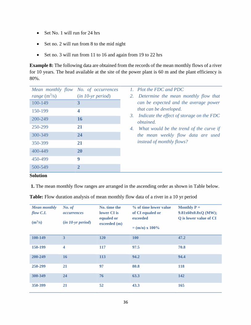
(i) The flow duration curve is obtained by plotting Q vs. percent of time in the Fig. (Q = lower
value of the CI.).
(ii) The power duration curve is obtained by plotting P vs. percent of time, see the Figure below.
2. The mean monthly flow that can be expected is the flow that is available for 50% of the time
i.e., 335 m3/s from the FDC drawn.
The average power that can be developed i.e., from the flow available for 50% of the time, is 157
MW, from the PDC drawn.
3. The effect of storage is to raise the flow duration curve on the dry weather portion and lower it
on the high flow portion and thus tends to equalize the flow at different times of the year, as
indicated in Fig. above.
4. If the mean weekly flow data are used instead of the monthly flow data, the flow duration curve
lies below the curve obtained from monthly flows for about 75% of the time towards the drier part
of the year and above it for the rest of the year as indicated in Figure above.
38
In fact the flow duration curve obtained from daily flow data gives the details more accurately
(particularly near the ends) than the curves obtained from weekly or monthly flow data but the
latter provide smooth curves because of their averaged out values.
Example 9: A run-of-river plant with an effective head of 22 m and plant efficiency of 80%
supplies power to a variable load as given below: Draw the load curve and determine
(i) The minimum average daily flow to supply the indicated load
(ii) Pondage required to produce the necessary power at the peak
(iii) The plant load factor
39
Solution
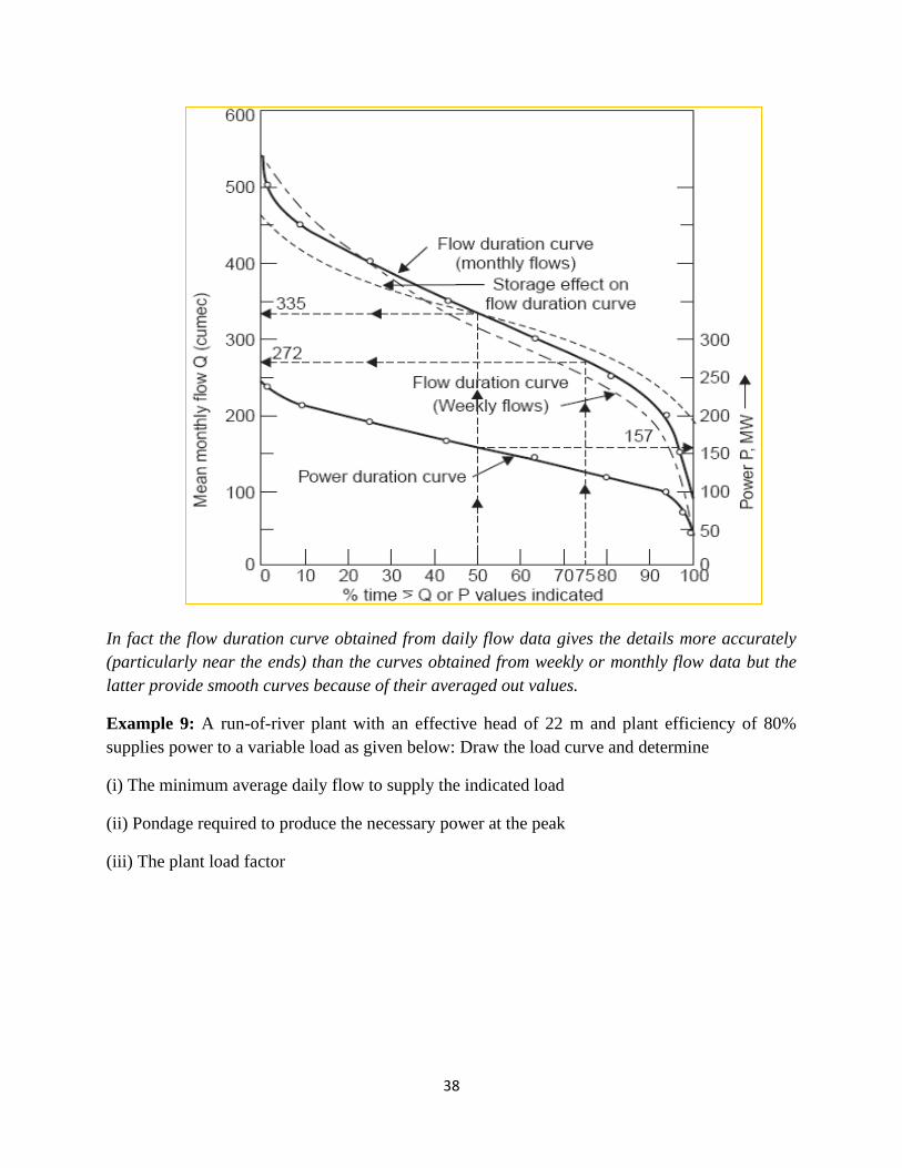
(i) The load curve is shown below.
• Total sum of loads at 2-hr intervals =
428.6 x 1000 kW
• Average load = (428.6 x 1000 kW x
2hr)/24hr = 35.72 MW
• Flow, Q, required to develop the
average load
→ Q = 35.72MW/(9.81x22x0.8) = 207 m3/s
(ii) Flow required to produce the required load/demand
Q = P in 1000 kW/(9.81x22x0.8) = 5.8 x Load in 1000 kW
To determine the pondage capacity the table below is prepared. From the table
Total deficiency = Total excess = 510 m3/s
Therefore, pondage capacity required = 510 m3/s for 2 hrs
= 510 x (2 x 60 x 60) = 3.67 x 10⁶ m3 or 3.67 Mm3
(iii) Plant load factor is the ratio of average load to peak load,
35.72/74.2 = 0.482
01020304050607080
0 2 4 6 8 10 12 14 16 18 20 22 24
Load
MW
Time (GMT)
Ave. Load = 35.72
Peak Load = 74.2Load Factor =
35.72/74.2 = 0.482
40
Time (hr) Load (MW) Required f
low (m3/s)
Deviation from the average flow of 207
m3/s
Deficiency Excess
0-2 11.4 66.1
140.90
2-4 5.6 32.46
174.54
4-6 25.6 148.4
58.60
6-8 53.2 308.2 101.2
8-10 44.8 260.0 53.0
10-12 39.4 228.5 21.5
12-14 44.2 256.0 49.0
14-16 44.4 257.4 50.4
16-18 74.2 430.0 223.0
18-20 37.8 219.4 12.4
20-22 30.0 174.0
33.0
22-24 18.0 104.3
102.7
Total 428.6
510.1 509.74
41
Chapter 3: Turbine selection and capacity determination Contents
1. Turbine types
2. Limits of Use of Turbine Types
3. Turbine selection criteria
1. Rotational speed
2. Specific speed
3. Maximum efficiency
4. Determination of Number of Units
5. Power house
3.1. Turbine types
Hydraulic Turbines transfer the energy from a flowing fluid to a rotating shaft. Turbine itself means
a thing which rotates or spins. Hydraulic Turbines have a row of blades fitted to the rotating shaft.
Flowing liquid, mostly water, when passes through the Turbine it strikes the blades of the turbine
and makes the shaft rotate.
For every specific use, a particular type of Hydraulic Turbine provides an optimum output. Thus
a hydro turbine is usually tailor made in order to fit a particular net hydraulic head and a design
flow discharge.
Turbines are classified based on Flow path or pressure change
Turbines types: Based on flow path
(i) Axial Flow Hydraulic Turbines: Hydraulic Turbines having the flow path of the water
mainly parallel to the axis of rotation.
(ii) Radial Flow Hydraulic Turbines: Hydraulic Turbines having the water flowing mainly
in a plane perpendicular to the axis of rotation.
(iii)Mixed Flow Hydraulic Turbines: Hydraulic Turbines having significant component of
both axial and radial flows. Francis Turbine is an example of mixed flow type, in Francis
Turbine water enters in radial direction and exits in axial direction.
None of the Hydraulic Turbines are purely axial flow or purely radial flow. There is always
a component of radial flow in axial flow turbines and of axial flow in radial flow turbines.
Turbine Types: Based on pressure change
One more important criterion for classification of Hydraulic Turbines is whether the pressure of
water changes or not while it flows through the runner of the Hydraulic Turbines. Based on the
pressure change Hydraulic Turbines can be classified as of two types.
42
(i) Impulse Turbine: The pressure of water does not change while flowing through the
runner. In Impulse Turbines pressure change occur only in the nozzles. One such
example of impulse turbine is Pelton Wheel.
(ii) Reaction Turbine: The pressure of water changes while it flows through the runner.
The change in water velocity and reduction in its pressure causes a reaction on the
turbine blades; this is where from the name Reaction Turbine may have been derived.
Francis and Propeller Turbines fall in the category of Reaction Turbines.
Turbine types: Reaction
In reaction turbines only a part of the inlet hydraulic energy is converted into velocity energy in
the stationary turbine parts. Thus, the conversion of hydraulic to mechanical energy in the runner
can be divided into two:
• The impulse action caused by the change of velocity direction from the runner inlet to the
outlet, and
• The reaction contribution caused by the pressure drop through the runner. The pressure
drop is obtained because the runner is completely filled with water. In the draft tube
(Connecting the outlet of the turbine runner to the tail race) some of the velocity energy at
the runner outlet is converted to potential energy.
Francis, Deriaz and propeller turbines belong to this group.
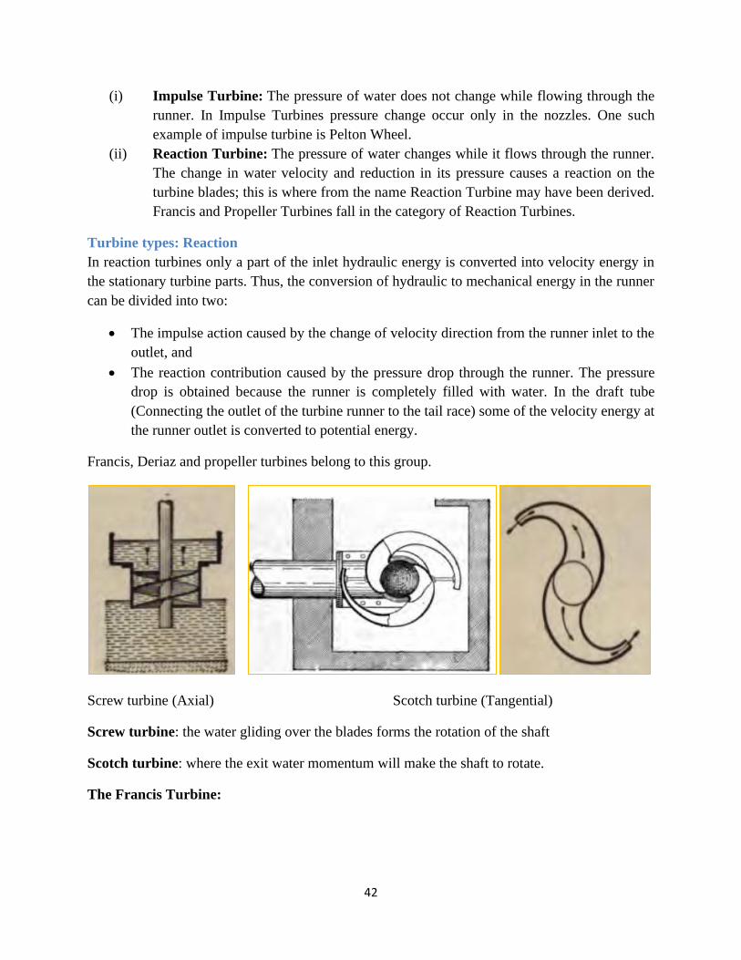
Screw turbine (Axial) Scotch turbine (Tangential)
Screw turbine: the water gliding over the blades forms the rotation of the shaft
Scotch turbine: where the exit water momentum will make the shaft to rotate.
The Francis Turbine:

43
• It is a reaction turbine developed by Sir J.B. Francis.
• The water enters the turbine through the outer periphery of the runner in the radial direction
and leaves the runner in the axial direction, and hence it is called ‘mixed flow turbine’.
• Only a part of the available hydraulic head is converted into the velocity head before water
enters the runner. The pressure head goes on decreasing as the water flows over the runner.
• The pressure at the runner exit may be less than the atmospheric pressure and thus water
fills all the passages of the runner.
• The change in pressure while water is gliding over the blades is called ‘reaction pressure’
and is partly responsible for the rotation of the runner.
• A Francis turbine is suitable for high heads (70 to 500 m) and requires a medium quantity
of water.
Propeller turbine
A propeller turbine generally has a runner with three to six blades in which the water contacts all
of the blades constantly. The pitch of the blades may be fixed or adjustable. The major components
besides the runner are a scroll case, wicket gates, and a draft tube. Types of propeller turbines:
• Bulb turbine: The turbine and generator are a sealed unit placed directly in the water
stream.
• Kaplan: Both the blades and the wicket gates are adjustable, allowing for a wider range of
operation.
• Other include Straflo and Tube turbines
Bulb Turbine

44
Used for very low head applications with a net head range from 0.5 to 30 m
The most important feature of a bulb turbine is the horizontal positioning of the shaft, which results
in a reduced size compared to a vertical shaft arrangement. After the intake, the water passes
through the moveable wicket gates, which are another device besides the runner for adjusting the
water discharge and, as a result, the turbine output. After passing the runner, the water exits from
the turbine through the draft tube. The generator is located in a watertight housing called the
“bulb”.
Small versions of the bulb turbine can be lowered into a stream by hand to power a remote home
Kaplan Turbine (Axial)
• It is a reaction turbine developed by Victor Kaplan ,1919
• The water enters the turbine through the outer periphery of the runner in the axial direction
and leaves the runner in the axial direction, and hence it is called ‘axial flow turbine’.
• Only a part of the available hydraulic head is converted into the velocity head before water
enters the runner. The pressure head goes on decreasing as the water flows over the runner
blades.
• The static pressure at the runner exit may be less than the atmospheric pressure and thus
water fills all the passages of the runner blades.
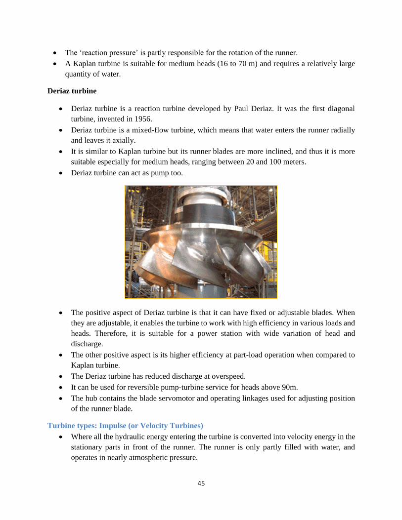
45
• The ‘reaction pressure’ is partly responsible for the rotation of the runner.
• A Kaplan turbine is suitable for medium heads (16 to 70 m) and requires a relatively large
quantity of water.
Deriaz turbine
• Deriaz turbine is a reaction turbine developed by Paul Deriaz. It was the first diagonal
turbine, invented in 1956.
• Deriaz turbine is a mixed-flow turbine, which means that water enters the runner radially
and leaves it axially.
• It is similar to Kaplan turbine but its runner blades are more inclined, and thus it is more
suitable especially for medium heads, ranging between 20 and 100 meters.
• Deriaz turbine can act as pump too.
• The positive aspect of Deriaz turbine is that it can have fixed or adjustable blades. When
they are adjustable, it enables the turbine to work with high efficiency in various loads and
heads. Therefore, it is suitable for a power station with wide variation of head and
discharge.
• The other positive aspect is its higher efficiency at part-load operation when compared to
Kaplan turbine.
• The Deriaz turbine has reduced discharge at overspeed.
• It can be used for reversible pump-turbine service for heads above 90m.
• The hub contains the blade servomotor and operating linkages used for adjusting position
of the runner blade.
Turbine types: Impulse (or Velocity Turbines)
• Where all the hydraulic energy entering the turbine is converted into velocity energy in the
stationary parts in front of the runner. The runner is only partly filled with water, and
operates in nearly atmospheric pressure.

46
• As the water enters/hits the turbine runner tangentially they are called Tangential flow
turbines
• All impulse turbines are tangential flow turbines
o The Pelton Turbine used for the highest heads
o Turgo impulse turbine
o Cross flow turbine (used in substitution of Francis turbine).
The Pelton Turbine: Patented by Lester Pelton 1880
Turgo Impulse turbine
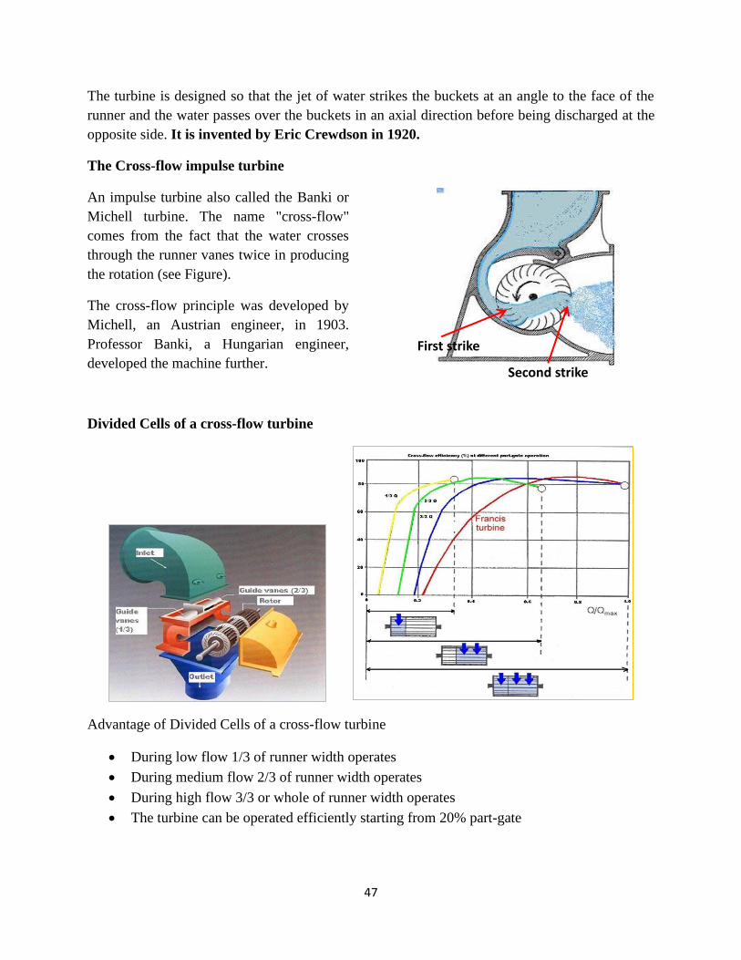
47
The turbine is designed so that the jet of water strikes the buckets at an angle to the face of the
runner and the water passes over the buckets in an axial direction before being discharged at the
opposite side. It is invented by Eric Crewdson in 1920.
The Cross-flow impulse turbine
An impulse turbine also called the Banki or
Michell turbine. The name "cross-flow"
comes from the fact that the water crosses
through the runner vanes twice in producing
the rotation (see Figure).
The cross-flow principle was developed by
Michell, an Austrian engineer, in 1903.
Professor Banki, a Hungarian engineer,
developed the machine further.
Divided Cells of a cross-flow turbine
Advantage of Divided Cells of a cross-flow turbine
• During low flow 1/3 of runner width operates
• During medium flow 2/3 of runner width operates
• During high flow 3/3 or whole of runner width operates
• The turbine can be operated efficiently starting from 20% part-gate
First strike
Second strike
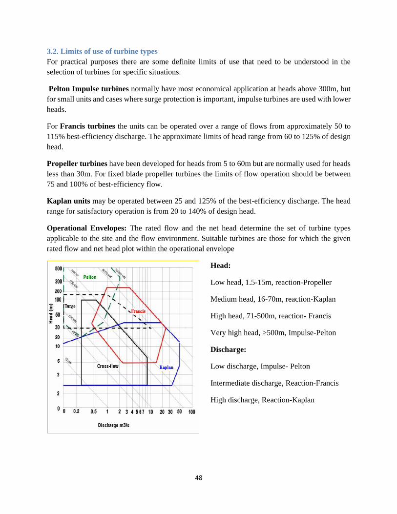
48
3.2. Limits of use of turbine types
For practical purposes there are some definite limits of use that need to be understood in the
selection of turbines for specific situations.
Pelton Impulse turbines normally have most economical application at heads above 300m, but
for small units and cases where surge protection is important, impulse turbines are used with lower
heads.
For Francis turbines the units can be operated over a range of flows from approximately 50 to
115% best-efficiency discharge. The approximate limits of head range from 60 to 125% of design
head.
Propeller turbines have been developed for heads from 5 to 60m but are normally used for heads
less than 30m. For fixed blade propeller turbines the limits of flow operation should be between
75 and 100% of best-efficiency flow.
Kaplan units may be operated between 25 and 125% of the best-efficiency discharge. The head
range for satisfactory operation is from 20 to 140% of design head.
Operational Envelopes: The rated flow and the net head determine the set of turbine types
applicable to the site and the flow environment. Suitable turbines are those for which the given
rated flow and net head plot within the operational envelope
Head:
Low head, 1.5-15m, reaction-Propeller
Medium head, 16-70m, reaction-Kaplan
High head, 71-500m, reaction- Francis
Very high head, >500m, Impulse-Pelton
Discharge:
Low discharge, Impulse- Pelton
Intermediate discharge, Reaction-Francis
High discharge, Reaction-Kaplan
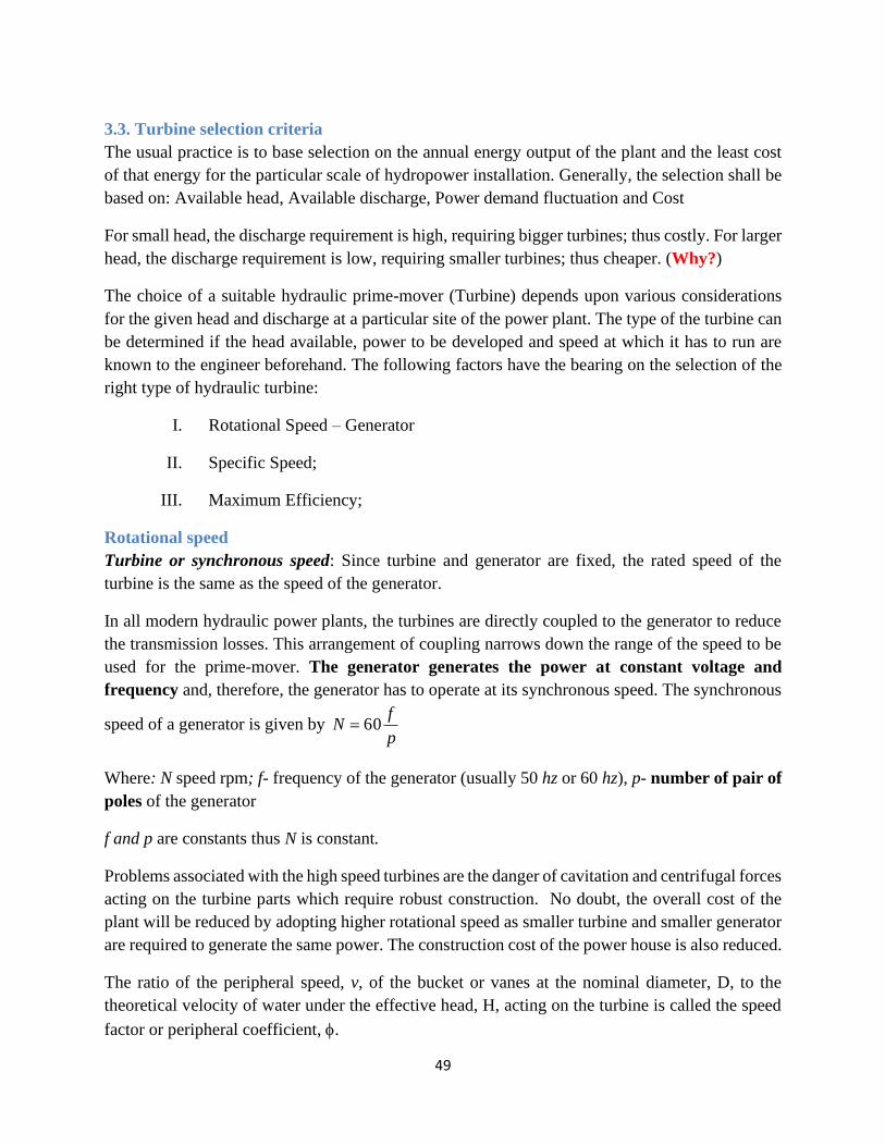
49
3.3. Turbine selection criteria
The usual practice is to base selection on the annual energy output of the plant and the least cost
of that energy for the particular scale of hydropower installation. Generally, the selection shall be
based on: Available head, Available discharge, Power demand fluctuation and Cost
For small head, the discharge requirement is high, requiring bigger turbines; thus costly. For larger
head, the discharge requirement is low, requiring smaller turbines; thus cheaper. (Why?)
The choice of a suitable hydraulic prime-mover (Turbine) depends upon various considerations
for the given head and discharge at a particular site of the power plant. The type of the turbine can
be determined if the head available, power to be developed and speed at which it has to run are
known to the engineer beforehand. The following factors have the bearing on the selection of the
right type of hydraulic turbine:
I. Rotational Speed – Generator
II. Specific Speed;
III. Maximum Efficiency;
Rotational speed
Turbine or synchronous speed: Since turbine and generator are fixed, the rated speed of the
turbine is the same as the speed of the generator.
In all modern hydraulic power plants, the turbines are directly coupled to the generator to reduce
the transmission losses. This arrangement of coupling narrows down the range of the speed to be
used for the prime-mover. The generator generates the power at constant voltage and
frequency and, therefore, the generator has to operate at its synchronous speed. The synchronous
speed of a generator is given by p
fN 60=
Where: N speed rpm; f- frequency of the generator (usually 50 hz or 60 hz), p- number of pair of
poles of the generator
f and p are constants thus N is constant.
Problems associated with the high speed turbines are the danger of cavitation and centrifugal forces
acting on the turbine parts which require robust construction. No doubt, the overall cost of the
plant will be reduced by adopting higher rotational speed as smaller turbine and smaller generator
are required to generate the same power. The construction cost of the power house is also reduced.
The ratio of the peripheral speed, v, of the bucket or vanes at the nominal diameter, D, to the
theoretical velocity of water under the effective head, H, acting on the turbine is called the speed
factor or peripheral coefficient, .
50
H
DN
gH
DN
gH
r
gH
v
6.8426022====
The following table suggests appropriate values of, which give the highest efficiencies for any
turbine, the head & specific speed ranges and the efficiencies of the three main types of turbine.
Type of runner Ns H (m) Efficiency (%)
Impulse 0.43 – 0.48 8-17
17
17-30
>250 85-90
90
90-82
Francis 0.6 – 0.9 40 – 130
130-350
350-452
25-450 90-94
94
94-93
Propeller 1.4 – 2.0 380-600
600-902
< 60 94
94-85
Cavitation
A reduced pressure under the blades (or buckets) of a turbine runner may lead to cavitation –
phenomenon detrimental to the turbine. The term cavitation basically refers to the ability of cold
water to boil under low pressure. Under a normal absolute barometric pressure of 1 bar water
starts to boil at 100 oC. However, when the pressure drops to 0.033 bar (which is called the critical
pressure, Pcr) it may begin to boil at 25 oC, that is, at normal river water temperature.
When the pressure under a runner approaches Pcr, the water in the stream starts boiling, giving rise
to cavities (known as cavitation bubbles) filled with water vapor.
The boundary between the low-pressure zone immediately under the blades (or buckets) and the
high-pressure zone in the stream above the runner follows an extremely unstable pattern. The
cavitation bubbles find themselves from time to time in the high-pressure zone. As a result, the
vapor instantly condenses and a cavitation bubble collapses. As this takes place, an enormous
pressure develops at the bubble center, which spreads quickly in an explosion-like manner.
A series of such micro-explosions following one another at very short intervals causes a good deal
of noise and vibration in the turbine and may provoke the runner blades into pitting.
Specific Speed
The turbine specific speed is a quantity derived from dimensional analysis. For a specific turbine
type (Francis, Kaplan, Pelton), the turbine efficiency will be primarily a function of specific speed.
Neglecting, the effect of hydraulic losses on the turbine power, the power will be given by:
QHP =
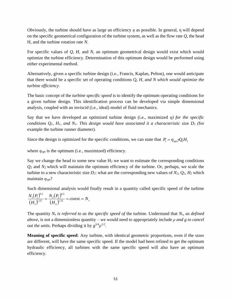
51
Obviously, the turbine should have as large an efficiency η as possible. In general, η will depend
on the specific geometrical configuration of the turbine system, as well as the flow rate Q, the head
H, and the turbine rotation rate N.
For specific values of Q, H, and N, an optimum geometrical design would exist which would
optimize the turbine efficiency. Determination of this optimum design would be performed using
either experimental method.
Alternatively, given a specific turbine design (i.e., Francis, Kaplan, Pelton), one would anticipate
that there would be a specific set of operating conditions Q, H, and N which would optimize the
turbine efficiency.
The basic concept of the turbine specific speed is to identify the optimum operating conditions for
a given turbine design. This identification process can be developed via simple dimensional
analysis, coupled with an inviscid (i.e., ideal) model of fluid mechanics.
Say that we have developed an optimized turbine design (i.e., maximized η) for the specific
conditions Q1, H1, and N1. This design would have associated it a characteristic size D1 (for
example the turbine runner diameter).
Since the design is optimized for the specific conditions, we can state that 111 HQP opt=
where ηopt is the optimum (i.e., maximized) efficiency.
Say we change the head to some new value H2 we want to estimate the corresponding conditions
Q2 and N2 which will maintain the optimum efficiency of the turbine. Or, perhaps, we scale the
turbine to a new characteristic size D2: what are the corresponding new values of N2, Q2, H2 which
maintain ηopt?
Such dimensional analysis would finally result in a quantity called specific speed of the turbine
( )( )
( )( ) sNconstH
PN
H
PN=== .
25.1
2
5.0
22
25.1
1
5.0
11
The quantity Ns is referred to as the specific speed of the turbine. Understand that Ns, as defined
above, is not a dimensionless quantity – we would need to appropriately include ρ and g to cancel
out the units. Perhaps dividing it by g5/4ρ1/2.
Meaning of specific speed: Any turbine, with identical geometric proportions, even if the sizes
are different, will have the same specific speed. If the model had been refined to get the optimum
hydraulic efficiency, all turbines with the same specific speed will also have an optimum
efficiency.
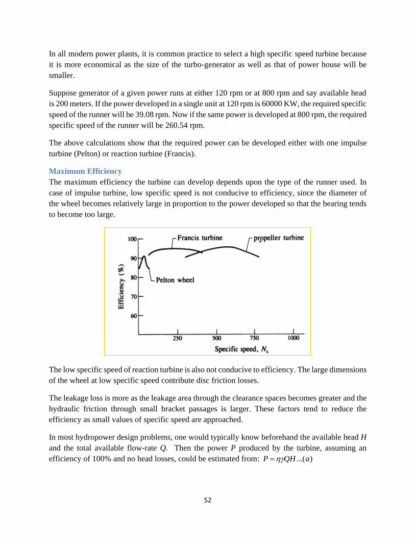
52
In all modern power plants, it is common practice to select a high specific speed turbine because
it is more economical as the size of the turbo-generator as well as that of power house will be
smaller.
Suppose generator of a given power runs at either 120 rpm or at 800 rpm and say available head
is 200 meters. If the power developed in a single unit at 120 rpm is 60000 KW, the required specific
speed of the runner will be 39.08 rpm. Now if the same power is developed at 800 rpm, the required
specific speed of the runner will be 260.54 rpm.
The above calculations show that the required power can be developed either with one impulse
turbine (Pelton) or reaction turbine (Francis).
Maximum Efficiency
The maximum efficiency the turbine can develop depends upon the type of the runner used. In
case of impulse turbine, low specific speed is not conducive to efficiency, since the diameter of
the wheel becomes relatively large in proportion to the power developed so that the bearing tends
to become too large.
The low specific speed of reaction turbine is also not conducive to efficiency. The large dimensions
of the wheel at low specific speed contribute disc friction losses.
The leakage loss is more as the leakage area through the clearance spaces becomes greater and the
hydraulic friction through small bracket passages is larger. These factors tend to reduce the
efficiency as small values of specific speed are approached.
In most hydropower design problems, one would typically know beforehand the available head H
and the total available flow-rate Q. Then the power P produced by the turbine, assuming an
efficiency of 100% and no head losses, could be estimated from: )...(aQHP =
53
The figure above could then be used, in conjunction with the head H and the estimated power P,
to determine the corresponding rotational speeds of Pelton, Francis, and Kaplan turbines operating
at their maximum efficiency, i.e., 5.0
25.1
P
HNN s=
An alternative approach is to specify beforehand the desired rotation rate N of the turbine. The
power produced by the three turbine types, operating at optimum efficiency, would then be
obtained by: 2
5.22
N
HNP s=
Q could then be calculated from Eq. (a), and the number of required turbine units would be
obtained from the total available flow rate divided by the flow through a single turbine.
3.4. Determination of number of units
It is cost effective to have a minimum number of units at a given installation; However, multiple
units may be necessary to make the most efficient use of water where flow variation is great.
Factors governing selection of number of units:
• Space limitations by geology or existing structure.
• Transportation facility
• Possibility of onsite fabrication
o Is costly and practical only for multiple units
o Runners may be split in two pieces, completely machined in the factory and bolted
together in the field. This is avoided as the integrity of the runner cannot be assured.
The current trend is to have small number of units having larger sizes, as larger sized units have a
better efficiency.
Example 1: Installed capacity needed: 1500 MW, set the number of turbine required.
Solution: This could have a number of alternatives on the number of units’ selection
• +1 units of 500 MW capacity
• +1 units of 300 MW capacity
• 8 +0 units of 200 MW capacity
• 1+1 unit of 1500 MW capacity
• Etc.
Example 2: A turbine is to operate under a head of 25 m at 200 rpm. The discharge is 9 m3/s. If
the efficiency is 90% determine the power generated; specific speed of the turbine and type of the
turbine.
Solution:

54
( )( )
( )( )
5.15925
523.1986200
523.198625981.99.0
25.1
5.0
25.1
5.0
===
===
H
PNN
KWQhP
s
As the specific speed lies between 60 and 400 Francis turbine is selected
Example 3: What type of turbine would be used if the discharge is of 0.283 m3/s with a head of
75m? Assume an efficiency of 80% and rotational speed of 600rpm.
Solution:
( )( )
( )( )
09.3575
6.166600
6.16675283.081.99.0
25.1
5.0
25.1
5.0
===
===
H
PNN
KWQhP
s
It would therefore be necessary to use a Fast Pelton Turbine. However, it might be possible to use
a Pelton Wheel with two jets.
Power per jet = 166.6/2 = 83.3KW. Therefore, Ns per Jet = 24.8 which is Medium speed Pelton
wheel.
If a Pelton Wheel with six jets is used:
Power per jet = 166.6/6 = 27.76KW. Therefore, Ns per Jet = 14.32 which is Slow speed Pelton
wheel. This would be a practical proposition but would result in some loss of efficiency due to
interference between the jets. Consequently, a better alternative would be to have two wheels on
the same shaft with two jets per wheel.
Example 4: In a hydropower station, water is available at a rate of 175 m3/s under a head of 18 m.
The turbines run at a speed of 150 rpm with overall efficiency of 82%. Find the number of turbines
required if they have the maximum specific speed of 460.
Solution
Specific speed of the turbine:
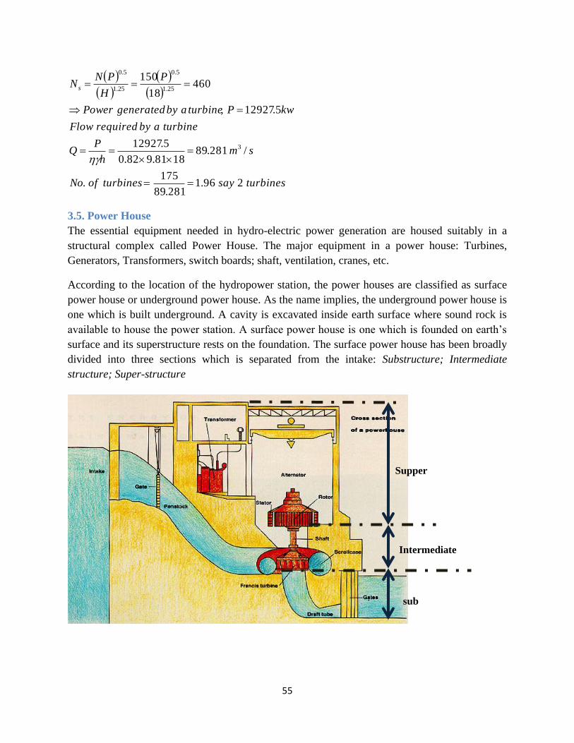
55
( )( )
( )( )
turbinessayturbinesofNo
smh
PQ
turbineabyrequiredFlow
kwPturbineabygeneratedPower
P
H
PNN s
296.1281.89
175.
/281.891881.982.0
5.12927
5.12927,
46018
150
3
25.1
5.0
25.1
5.0
==
=
==
=
===
3.5. Power House
The essential equipment needed in hydro-electric power generation are housed suitably in a
structural complex called Power House. The major equipment in a power house: Turbines,
Generators, Transformers, switch boards; shaft, ventilation, cranes, etc.
According to the location of the hydropower station, the power houses are classified as surface
power house or underground power house. As the name implies, the underground power house is
one which is built underground. A cavity is excavated inside earth surface where sound rock is
available to house the power station. A surface power house is one which is founded on earth’s
surface and its superstructure rests on the foundation. The surface power house has been broadly
divided into three sections which is separated from the intake: Substructure; Intermediate
structure; Super-structure
Intermediate
sub
Supper
56
Substructure
The substructure of a power-house is defined as that part which extends from the bottom of the
turbine to the soil or rock. Its purpose is to house the passage for the water coming out of the
turbine.
Hydraulic function
In case of reaction turbines the substructure is used to provide a diverging passage (draft tube)
where the velocity of the exit water is gradually reduced in order to reduce the loss in pushing out
the water. In case of impulse turbine, such a draft tube is not required and only an exit gallery
would serve the purpose.
Structural function is dual:
• To safely carry the superimposed loads of machines and other structures over the cavities.
• To act as transition foundation member that distributes heavy machine loads on the soil
such that the obtainable ground pressures are within safe limits.
Intermediate structure
The intermediate structure is part of the power house which extends from the top of the draft tube
to top of the generator foundation.
This structure contains two important elements of the power house, one is the scroll case which
feeds water to the turbine. The generator foundation rests on the scroll-case which is embedded in
the concrete. Other galleries and chambers also rest on the same foundation.
Scroll or spiral case (for reaction turbine only) is a part of the turbine that distributes water coming
from penstock uniformly and smoothly through guide vanes to the turbine. In case of impulse
turbine manifold supplying water to the nozzles will serve this purpose.
The structural function of the generator foundation in the intermediate structure is to support the
generator. Arrangements may be made either to transmit the load directly to the substructure
through steel barrel or through a column beam or slab.
The structural function of the concrete around scroll case would depend upon the type of scroll
case used:
If the scroll case is made of steel and strong enough to withstand internal loads including the water
hammer effects, the surrounding concrete acts more or less as a space fill and a medium to
distribute the generator loads to the substructure.
If it is a concrete scroll case then this concrete should be strong enough to withstand the internal
hydrostatic and water hammer head as well as the external superimposed loads on account of the
machine etc. Usually, a steel scroll case is used as water linear.
57
Superstructure:
The part of the power house above the generator floor right up to the roof is known as
superstructure. This part provides walls and roofs to power station and also provides an overhead
travelling crane for handling heavy machine parts.
Power House Dimensions
Length: depends on the number of units installed; the units shall be spaced at
• 5D + 2.5m where D is the turbine outer diameter
• 4D + 2.5m for high specific speed turbines
• Additional length is provided for loading/erection and control room is required
Width: equal to the center to center spacing of the units plus the clearance space from the wall
Height: fixed by the head room requirements of the crane operation.
Underground power house
Depending on the rock quality, tunneling ease, overall economics, and the power house may be
located:
• The plant totally underground
• In a pit: the PH is accessed from the surface
• Semi-underground: turbine in the ground while generator is on the surface
• In a rock cut
Advantages:
• Shorter underground conduit
• Cheaper penstock design
• Favorable construction conditions
• Preserve the landscape
Disadvantages
Higher construction cost
Higher operational cost
The lighting cost.
The running cost of air-conditioned plant.
The removal of water seeping
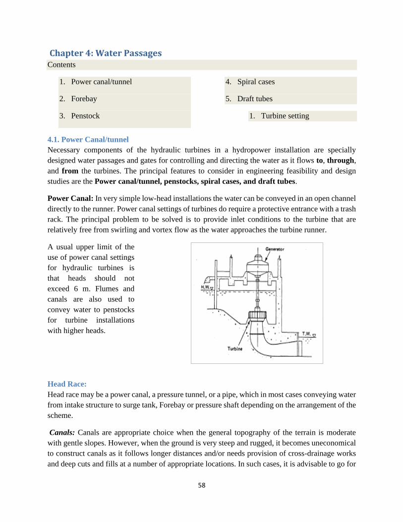
58
Chapter 4: Water Passages Contents
1. Power canal/tunnel
2. Forebay
3. Penstock
4. Spiral cases
5. Draft tubes
1. Turbine setting
4.1. Power Canal/tunnel
Necessary components of the hydraulic turbines in a hydropower installation are specially
designed water passages and gates for controlling and directing the water as it flows to, through,
and from the turbines. The principal features to consider in engineering feasibility and design
studies are the Power canal/tunnel, penstocks, spiral cases, and draft tubes.
Power Canal: In very simple low-head installations the water can be conveyed in an open channel
directly to the runner. Power canal settings of turbines do require a protective entrance with a trash
rack. The principal problem to be solved is to provide inlet conditions to the turbine that are
relatively free from swirling and vortex flow as the water approaches the turbine runner.
A usual upper limit of the
use of power canal settings
for hydraulic turbines is
that heads should not
exceed 6 m. Flumes and
canals are also used to
convey water to penstocks
for turbine installations
with higher heads.
Head Race:
Head race may be a power canal, a pressure tunnel, or a pipe, which in most cases conveying water
from intake structure to surge tank, Forebay or pressure shaft depending on the arrangement of the
scheme.
Canals: Canals are appropriate choice when the general topography of the terrain is moderate
with gentle slopes. However, when the ground is very steep and rugged, it becomes uneconomical
to construct canals as it follows longer distances and/or needs provision of cross-drainage works
and deep cuts and fills at a number of appropriate locations. In such cases, it is advisable to go for
59
tunnels or pipes. The choice, in fact, has to be made based on economic analysis. Where the
topography of the region presents special formations, the alternating use of open-canal and open-
surface tunnel sections may ensure the most economical development.
Canal Design: Involves determination of the following:
• Carrying capacity, velocity of water in the canal & roughness coefficient of the canal
surface
• Canal slopes
• Cross-sectional profile of the canal
i) Carrying Capacity and Velocity:
The discharge is computed from continuity equation as Q = VA
The roughness coefficient is specified from the bed material type.
Chezy's equation: RSCV =
To determine the value of C we can use.
• Manning's Formula 6/11R
nC =
o Where n is Manning's roughness coefficient
• The Chezy-Manning equation
• Kutter Formula 2/13/22/13/21SMRSR
nV ==
• The Agroskin formula
Apart from the hydraulic computations, the flow velocities in the canal or other water conduits in
general are determined according to economic point of views (investments, head losses, wear and
tear of material, danger of erosion and silting).
The velocity must be high enough to prevent sedimentation. It has to be low enough to prevent
bed erosion for unlined-canals and wear by abrasion for lined-canals.
Maximum velocity Maximum velocity Minimum velocity
Vmin (m/s) Bed Material Vmax (m/s) Bed Material Vmax (m/s)
Sand
Loam
Clayey loam
0.4
0.6
0.8
Gravel
Masonry
Asphalt
3.0
3.5
4.0
To keep any sediment
from settling out, the
minimum velocity in a
canal should not be less
than 0. 3 m/s.
60
Clay 2.0 Concrete 5.0
Lowering the velocity keeps the head loss over the length of the canal to a minimum; however, it
increases the cost necessary to construct the canal as the cross-sectional area increases when the
velocity lowers.
In unlined canals flow velocities are limited by the resistance of the bed material to erosion. In
lined canals flow velocities are limited by resistance against wear.
Maximum Velocities
Critical bottom velocity (w.r.t. erosion) is given by:
1. Strenberg: dVb 2= for d is particle size in meters, ζ = 4.43
2. Maximum permissible mean velocity according to Bogardi and Yen is given by:
19.22 9/4 −= sm SdV
o Where dm is mean particle size and Ss is specific gravity of particles.
Minimum Velocities
There are various recommendations for non silting velocity
1) According to Ludin
• If Vmin > 0.3 m/sec, there will be no silting (for silty sediments)
• Vmin > 0.3 to 0.5 m/sec, there will be no silting (for sandy sediments)
2) According to R.C. Kennedy
• Non-scouring and non silting velocity is given by:
• Where h is depth of water in meters and C is coefficient varying from 0.54 to 0.7,
depending on silt load.
ii) Roughness coefficient
As water flows in a canal, it loses its energy in the process of sliding past the walls and bed
material. The rougher the material, the more frictional loss and the greater the head drop or slope
needed for a given velocity. The roughness coefficient, n, for various canal materials can be found
in standard open channel books.
iii) Power Canal Slopes
In plain areas slope between 5 to 20 cm/km are in use. In mountainous areas slopes are as steep as
1 to 2 m/km. The canal bed slope can also be estimated using the Manning’s equation:
3/4
22
R
VnS =
61
The slope found from the above equation should nearly coincide with the available natural
topography. Otherwise, a different slope should be computed by choosing other values for the
velocity within the permissible limit until a satisfactory result is obtained.
iv) Cross-sectional Profile:
The material in which the canal is constructed generally dictates its cross-sectional profile. The
common cross-sections used for canals are described in the following paragraphs.
• A rectangular cross-section is often most appropriate when excavation is undertaken in firm
rock. It is also commonly used when the canal incorporates properly constructed masonry
walls. Use of a rectangular canal reduces the excavation required. For the most efficient
rectangular cross-section, the width of the canal is twice the depth of the wetted area and, like
a trapezoidal section, is a section in which a semi-circle can be inscribed.
• A semi-circular cross-section is the most efficient profile because, for a given canal slope and
cross-sectional area, it conveys the maximum flow. However, this form is impractical to
excavate. It is therefore used primarily with materials which lend themselves to this shape.
Examples are prefabricated concrete, sheet metal, and wood-stave sections.
• A trapezoidal cross-section is the most widely used profile for both lined and unlined canals
excavated in earth. If the canal is unlined, the maximum side slope is set by that slope at which
the material will permanently stand under water. The magnitude of the side slope of a lined
trapezoidal canal depends on the nature of the material on which the lining will rest, but
usually steeper than unlined canals. In general, it should be nearly equal to the angle of repose
of the natural soil so that no earth pressure is exerted on the back of the lining. The banks of
a lined canal, resting on almost any free-draining material requires slopes not steeper than 1:1.
For a trapezoidal canal with a given side slope, the most efficient cross-section is one in which
a semi-circle can be inscribed in the wetted area. For this section, it can be shown that the
length of either sloping side of the wetted area is half its top width.
Freeboard Allowance:
For earth canal the lower limit is 35 cm and the upper limit is 140 cm. Generally the free board =
[0.35+1/4h] m. Where h is depth of flow. Allowances should be made for bank settlements.
For lined canals, the top of the lining is not usually extended for the full height of the free board.
Usually it is extended to 15cm to 70cm above the design water level.
Water Loss in Power Canals
Water losses are due to
a) Seepage
b) Evaporation
c) Leakage at gates
Generally b) and c) are of minor importance.

62
Tunnels
Tunnels are underground conveyance structures. A name tunnel indicates a very small bottom
slope, i.e. tunnels are aligned nearly horizontal. Shaft is a tunnel with vertical alignment or inclined
shaft when it is steeply inclined to the horizontal.
Tunneling is popular in hydropower because:
• It provides a direct and short route for the water passage thus resulting in considerable
saving in cost
• Tunneling work can be started simultaneously at many points thus leading to quicker
completion
• Natural land scape is not disturbed
• Development of new techniques of drilling & blasting, rock mechanics and machines.
Tunnels of hydropower projects fall into two categories: service tunnels and water carrying
tunnels.
Service tunnels: These may be:
• Cable tunnels: to carry cables from underground power house to the switch yard
• Ventilation tunnels: fitted with fans at the open end to supply fresh air to the underground
• Access or approach tunnels: this is a passage tunnel from surface to underground power
house.
Water carrying tunnels: Flows in water tunnels are usually under pressure (pipe flow), but
sometimes free-flow (open channel flow) can be experienced, especially, in tailrace tunnels. The
design of free-flow tunnels follows the same principles as used in the design of open canals.
Water carrying tunnels include:
• Head race/power tunnels: are tunnels that convey water to the surge tank. These are pressure
tunnels
• Tail race tunnels: could be free flowing or pressure tunnels depending on the relative position
of turbine setting and tail water level.
• Diversion tunnels: are constructed for the purpose of diverting the stream flow during
construction period. Normally they are not of high pressure but should have sufficient flood
carrying capacity. Such tunnels either plugged with concrete or converted in to some use
such as spillway tunnel at the completion of the project.
Classification of Tunnels
In addition to the above classification tunnels may be classified on the basis of alignment, shape
and design aspects.
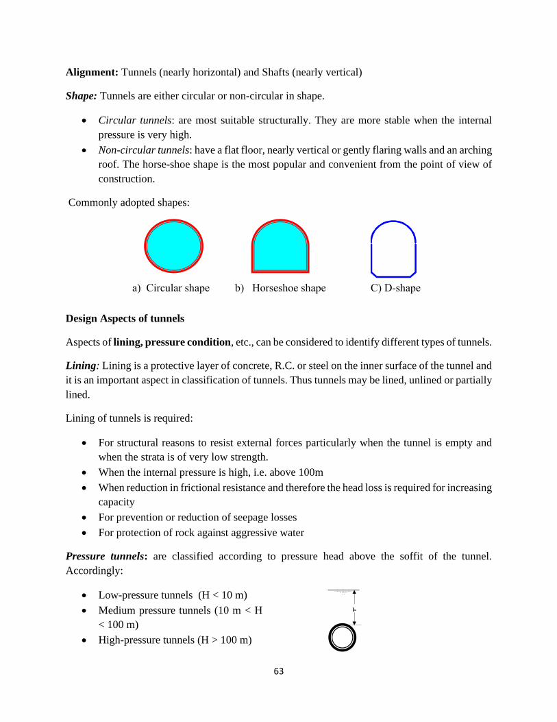
63
Alignment: Tunnels (nearly horizontal) and Shafts (nearly vertical)
Shape: Tunnels are either circular or non-circular in shape.
• Circular tunnels: are most suitable structurally. They are more stable when the internal
pressure is very high.
• Non-circular tunnels: have a flat floor, nearly vertical or gently flaring walls and an arching
roof. The horse-shoe shape is the most popular and convenient from the point of view of
construction.
Commonly adopted shapes:
Design Aspects of tunnels
Aspects of lining, pressure condition, etc., can be considered to identify different types of tunnels.
Lining: Lining is a protective layer of concrete, R.C. or steel on the inner surface of the tunnel and
it is an important aspect in classification of tunnels. Thus tunnels may be lined, unlined or partially
lined.
Lining of tunnels is required:
• For structural reasons to resist external forces particularly when the tunnel is empty and
when the strata is of very low strength.
• When the internal pressure is high, i.e. above 100m
• When reduction in frictional resistance and therefore the head loss is required for increasing
capacity
• For prevention or reduction of seepage losses
• For protection of rock against aggressive water
Pressure tunnels: are classified according to pressure head above the soffit of the tunnel.
Accordingly:
• Low-pressure tunnels (H < 10 m)
• Medium pressure tunnels (10 m < H
< 100 m)
• High-pressure tunnels (H > 100 m)
a) Circular shape b) Horseshoe shape C) D-shape
H
64
Low Head Tunnels
• The trimmed rock surface may be sufficient by only sealing visible fissure with concrete
or cement mortar or granite layer.
• Full lining may be warranted only if external rock load or aggressivity or water head loss
reduction justifies it.
Medium head Tunnels
• A water tight lining concrete is almost always needed since seepage is more likely to occur
under increasing head.
• If the lining is only for water sealing purposes, and no load is carried by it, the permissible
internal water pressure head is determined by the depth of overburden and the quality of
the rock.
• If depth of overburden rock is hr, Internal pressure head of water is H and r & w are
specific weight of the rock and water, then for equilibrium: w H r hr; With w = 1 ton/m3,
H r hr;
o Using a factor of safety of , ( )mh
H rr
=
o Where factor of safety = 4 to 6.
o With r = 2.4 t/m3 to 3.2 t /m3 and using lower values for good quality rock, one
gets H = (0.4 to 0.8) hr
High Head Pressure Tunnels
• Usually steel lining is used (R.C. Concrete lining not satisfactory)
• The steel lining is embedded in concrete filling the annular space b/n the steel lining & the
rock. In order to provide proper contact b/n rock and concrete and b/n steel lining &
concrete, all voids are filled by grouting with cement mortar.
• The profile of the Pressure tunnel should be such that the roof should always be at least 1
to 2m below the hydraulic grade line
In tunnel design:
• Saddles should be provided with dewatering provisions and summits should be provided
with outlets or shafts.
• To reduce construction costs, relatively high velocities (higher than in open channels) are
permitted in tunnels.
• The permissible velocity depends upon the sediment load carried by the water.
• Size of tunnels cannot be reduced arbitrarily. Requirements of passability limit the
maximum size.
o Minimum size of Tunnel: Circular, 1.8 m ; Rectangular, 2m x 1.6m.
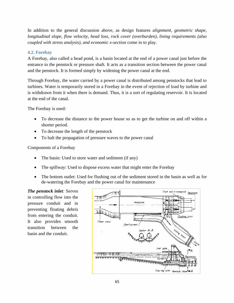
65
In addition to the general discussion above, as design features alignment, geometric shape,
longitudinal slope, flow velocity, head loss, rock cover (overburden), lining requirements (also
coupled with stress analysis), and economic x-section come in to play.
4.2. Forebay
A Forebay, also called a head pond, is a basin located at the end of a power canal just before the
entrance to the penstock or pressure shaft. It acts as a transition section between the power canal
and the penstock. It is formed simply by widening the power canal at the end.
Through Forebay, the water carried by a power canal is distributed among penstocks that lead to
turbines. Water is temporarily stored in a Forebay in the event of rejection of load by turbine and
is withdrawn from it when there is demand. Thus, it is a sort of regulating reservoir. It is located
at the end of the canal.
The Forebay is used:
• To decrease the distance to the power house so as to get the turbine on and off within a
shorter period.
• To decrease the length of the penstock
• To halt the propagation of pressure waves to the power canal
Components of a Forebay
• The basin: Used to store water and sediment (if any)
• The spillway: Used to dispose excess water that might enter the Forebay
• The bottom outlet: Used for flushing out of the sediment stored in the basin as well as for
de-watering the Forebay and the power canal for maintenance
The penstock inlet: Serves
in controlling flow into the
pressure conduit and in
preventing floating debris
from entering the conduit.
It also provides smooth
transition between the
basin and the conduit.
66
Design Guidelines for a Forebay
The location of the Forebay is primarily governed by topographic conditions and the geology of
the site. The site of both the Forebay and the powerhouse should be selected simultaneously with
a view of ensuring the shortest possible penstocks/pressure shafts.
The entire basin of the Forebay may be either excavated in rock or constructed above the terrain,
enclosed by embankments and retaining walls. The size of a Forebay varies depending on the
sediment content of the water conveyed in the power canal and whether it is to serve for storage.
It is not advisable to design the Forebay as a settling basin if the suspended sediment is fine to
cause no damage to the turbines. A gradual transition section should be provided between the
power canal and the Forebay basin. In the case of wide Forebay, baffle piers are usually
constructed at the basin inlet in order to ensure even distribution of flow to the basin.
The bottom of the Forebay basin should be provided with a proper slope to enable periodical
flushing of the silt deposited. A bottom lining of the Forebay basin is required in soils where large
seepage is expected. The smoothed bottom of the basin is covered with plastic clay having
thickness of 20 to 50 cm. The cover is compacted in several layers and is protected against
disturbance due to soaking and wave action by a layer of gravel or crushed stone.
The spillway is usually an ogee type with stilling basin. If the discharge to be taken care of is great
and if, at the same time, prevailing conditions do not permit the construction of a long overflow
weir, water surface regulation within narrow limits can be attained by constructing a siphon type
spillway. The spillway and the bottom outlet canal should be combined immediately at the foot of
the basin. Water spilling over the spillway crest and through the bottom outlet can be either
diverted into a suitable river bed (if any) in a nearby side valley or conveyed by a special chute.
In designing a Forebay tank, it is important to keep the entrance to the penstock fully submerged.
This is to prevent air being drawn in to the penstock because of a vortex which can be formed if
the penstock entrance is closer to the water surface in the basin.
The usual components of the intake such as trash racks, flow control devices (gates or valves), etc.
must be provided at the penstock inlet. It is necessary to install an air vent behind the gate to
prevent damage to the penstock if for some reason the penstock entrance is blocked or the gate is
suddenly closed causing a low pressure inside the conduit which can make it collapse inwards.
The air vent can also help remove air from inside the penstock during startup.
4.3. Penstock
A penstock is the conduit that is used to carry water from the supply sources to the turbine. This
conveyance is usually from a canal or reservoir. Penstocks classified based operation conditions:
• Pressure penstock: requires that the water discharging to the turbine always be under a
positive pressure (greater than atmospheric pressure).

67
• Siphon penstock: is constructed in such a way that at points in the penstock the pressure
may be less than atmospheric pressure and sections of the conduit act as a siphon. This
requires that a vacuum pump or some other means for initiating the siphon action must be
used to fill the conduit with water and to evacuate the air in the conduit.
Penstocks may be classified according to type of construction:
• Steel penstocks: the most common type of installation, due to simplicity in fabrication,
strength, and assurance that they will perform in a wide variety of circumstances. Normal
practice is to use welded steel pipe sections.
• Cast-in-place or precast reinforced concrete pipe: Very large diameters are somewhat
impractical. Cast-in-place concrete pipes are usually limited to heads of less than 35 m.
According to Creager and Justin (1950), these penstocks can be used up to 4m in diameter
and under heads up to 185 m by using a welded steel shell embedded in the reinforced
concrete.
• Fiberglass and polyvinyl chloride (PVC) plastic pipe: A penstock at the Niagara
Mohawk plant uses a fiberglass pipe 3 m in diameter.
• Wood stave pipes have been used in diameters ranging from 15 cm up to 6 m and utilized
at heads up to 185 m with proper design.
Safe Penstock Thickness
The thickness of the pipe shell (s) for penstocks should be determined by: s = PD/(2ησ); where s
= penstock shell thickness; P = internal pressure; D = pipe diameter; η = joint efficiency of welded
or riveted joint; σ = allowable unit stress of hoop tension. The allowable equivalent unit stress for
hoop tension will vary with the type of steel used in the penstock.
Minimum thickness (in inches), based on need for stiffness, corrosion protection, and strength
requirements, is indicated by the U.S. Department of the Interior (1967) to be:
smin= (D + 20)/400.
Size Selection of Penstocks
Various experience curves and empirical equations have been developed for determining the
economical size of penstocks. Some of these equations use very few parameters to make initial
size determinations for reconnaissance or feasibility studies. Other more sophisticated equations
use many variables to obtain more precise results which may be necessary for final design.
Economical size varies with type of installation and materials, as well as whether it is used above
ground or buried.
• Gordon and Penman (1979) give a very simple equation for determining steel penstock
diameter for small hydropower installations: Dp=0.72Q0.25
• Sarkaria (1979) developed an empirical approach for determining steel penstock diameter by
using data from large hydro projects with heads varying from 57 m to 313 m and power
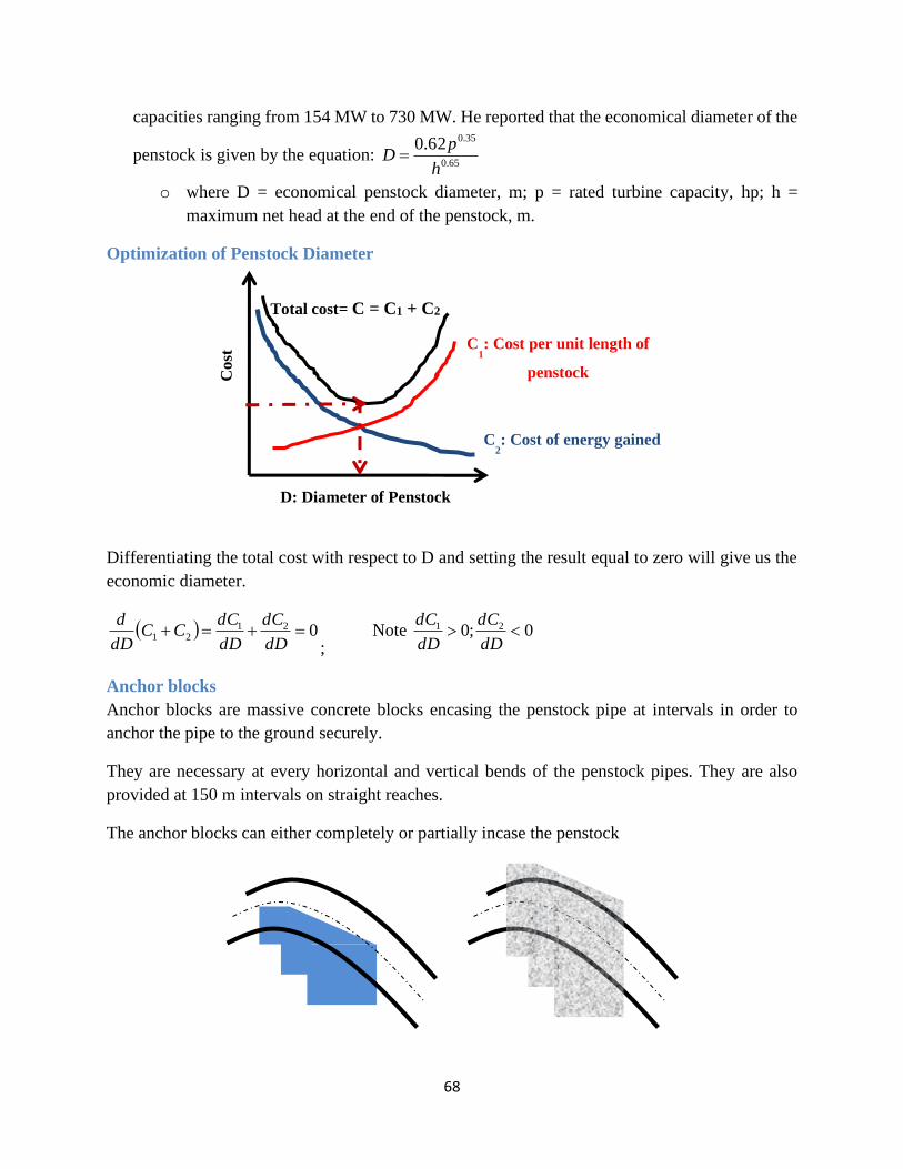
68
capacities ranging from 154 MW to 730 MW. He reported that the economical diameter of the
penstock is given by the equation: 65.0
35.062.0
h
pD =
o where D = economical penstock diameter, m; p = rated turbine capacity, hp; h =
maximum net head at the end of the penstock, m.
Optimization of Penstock Diameter
Differentiating the total cost with respect to D and setting the result equal to zero will give us the
economic diameter.
( ) 02121 =+=+
dD
dC
dD
dCCC
dD
d
; Note 0;0 21
dD
dC
dD
dC
Anchor blocks
Anchor blocks are massive concrete blocks encasing the penstock pipe at intervals in order to
anchor the pipe to the ground securely.
They are necessary at every horizontal and vertical bends of the penstock pipes. They are also
provided at 150 m intervals on straight reaches.
The anchor blocks can either completely or partially incase the penstock
D: Diameter of Penstock
Co
st
C2: Cost of energy gained
C1: Cost per unit length of
penstock
Total cost= C = C1 + C2
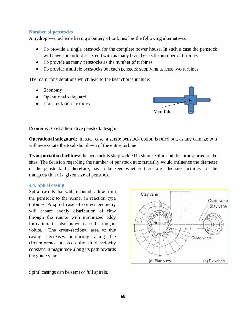
69
Number of penstocks
A hydropower scheme having a battery of turbines has the following alternatives:
• To provide a single penstock for the complete power house. In such a case the penstock
will have a manifold at its end with as many branches as the number of turbines.
• To provide as many penstocks as the number of turbines
• To provide multiple penstocks but each penstock supplying at least two turbines
The main considerations which lead to the best choice include:
• Economy
• Operational safeguard
• Transportation facilities
Economy: Cost /alternative penstock design/
Operational safeguard: in such case, a single penstock option is ruled out, as any damage to it
will necessitate the total shut down of the entire turbine
Transportation facilities: the penstock is shop welded in short section and then transported to the
sites. The decision regarding the number of penstock automatically would influence the diameter
of the penstock. It, therefore, has to be seen whether there are adequate facilities for the
transportation of a given size of penstock.
4.4. Spiral casing
Spiral case is that which conduits flow from
the penstock to the runner in reaction type
turbines. A spiral case of correct geometry
will ensure evenly distribution of flow
through the runner with minimized eddy
formation. It is also known as scroll casing or
volute. The cross-sectional area of this
casing decreases uniformly along the
circumference to keep the fluid velocity
constant in magnitude along its path towards
the guide vane.
Spiral casings can be semi or full spirals.
Manifold
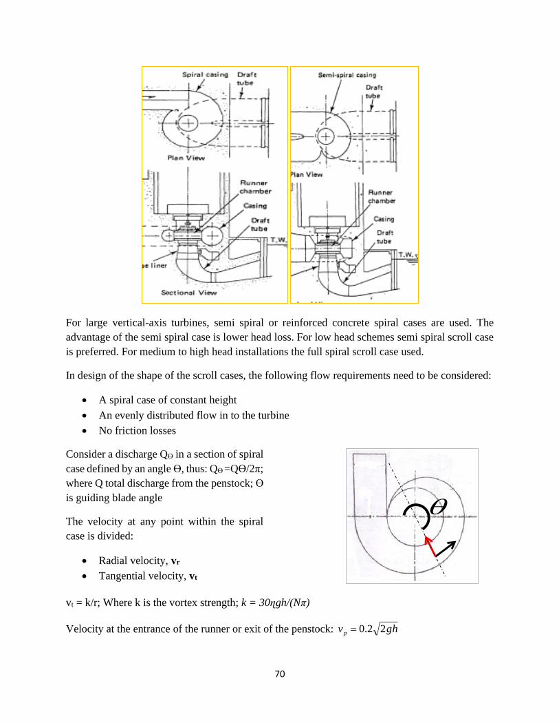
70
For large vertical-axis turbines, semi spiral or reinforced concrete spiral cases are used. The
advantage of the semi spiral case is lower head loss. For low head schemes semi spiral scroll case
is preferred. For medium to high head installations the full spiral scroll case used.
In design of the shape of the scroll cases, the following flow requirements need to be considered:
• A spiral case of constant height
• An evenly distributed flow in to the turbine
• No friction losses
Consider a discharge Qϴ in a section of spiral
case defined by an angle ϴ, thus: Qϴ =Qϴ/2π;
where Q total discharge from the penstock; ϴ
is guiding blade angle
The velocity at any point within the spiral
case is divided:
• Radial velocity, vr
• Tangential velocity, vt
vt = k/r; Where k is the vortex strength; k = 30ɳgh/(Nπ)
Velocity at the entrance of the runner or exit of the penstock: ghvp 22.0=
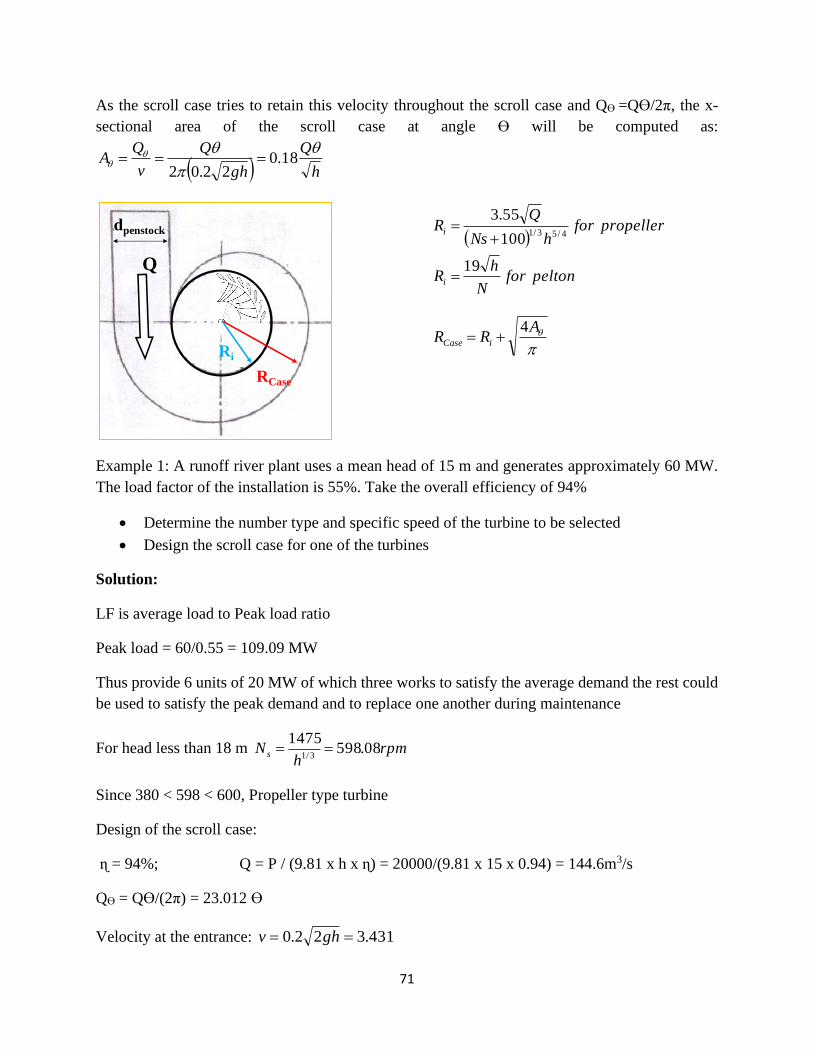
71
As the scroll case tries to retain this velocity throughout the scroll case and Qϴ =Qϴ/2π, the x-
sectional area of the scroll case at angle ϴ will be computed as:
( ) h
Q
gh
Q
v
QA
18.0
22.02===
( )
peltonforN
hR
propellerforhNs
QR
i
i
19
100
55.34/53/1
=
+=
A
RR iCase
4+=
Example 1: A runoff river plant uses a mean head of 15 m and generates approximately 60 MW.
The load factor of the installation is 55%. Take the overall efficiency of 94%
• Determine the number type and specific speed of the turbine to be selected
• Design the scroll case for one of the turbines
Solution:
LF is average load to Peak load ratio
Peak load = 60/0.55 = 109.09 MW
Thus provide 6 units of 20 MW of which three works to satisfy the average demand the rest could
be used to satisfy the peak demand and to replace one another during maintenance
For head less than 18 m rpmh
N s 08.5981475
3/1==
Since 380 < 598 < 600, Propeller type turbine
Design of the scroll case:
ɳ = 94%; Q = P / (9.81 x h x ɳ) = 20000/(9.81 x 15 x 0.94) = 144.6m3/s
Qϴ = Qϴ/(2π) = 23.012 ϴ
Velocity at the entrance: 431.322.0 == ghv
RCase
Ri
dpenstock
Q
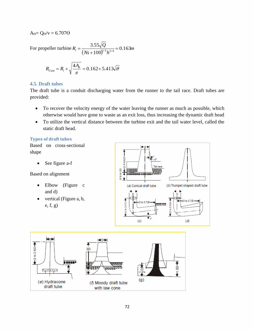
72
Aϴ= Qϴ/v = 6.707ϴ
For propeller turbine( )
mhNs
QRi 163.0
100
55.34/53/1=
+=
413.5162.04
+=+=A
RR iCase
4.5. Draft tubes
The draft tube is a conduit discharging water from the runner to the tail race. Draft tubes are
provided:
• To recover the velocity energy of the water leaving the runner as much as possible, which
otherwise would have gone to waste as an exit loss, thus increasing the dynamic draft head
• To utilize the vertical distance between the turbine exit and the tail water level, called the
static draft head.
Types of draft tubes
Based on cross-sectional
shape
• See figure a-f
Based on alignment
• Elbow (Figure c
and d)
• vertical (Figure a, b,
e, f, g)
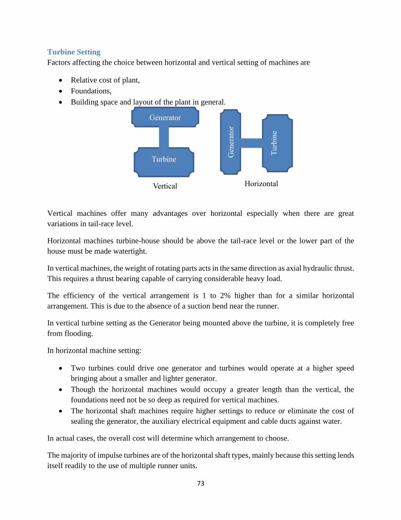
73
Turbine Setting
Factors affecting the choice between horizontal and vertical setting of machines are
• Relative cost of plant,
• Foundations,
• Building space and layout of the plant in general.
Vertical machines offer many advantages over horizontal especially when there are great
variations in tail-race level.
Horizontal machines turbine-house should be above the tail-race level or the lower part of the
house must be made watertight.
In vertical machines, the weight of rotating parts acts in the same direction as axial hydraulic thrust.
This requires a thrust bearing capable of carrying considerable heavy load.
The efficiency of the vertical arrangement is 1 to 2% higher than for a similar horizontal
arrangement. This is due to the absence of a suction bend near the runner.
In vertical turbine setting as the Generator being mounted above the turbine, it is completely free
from flooding.
In horizontal machine setting:
• Two turbines could drive one generator and turbines would operate at a higher speed
bringing about a smaller and lighter generator.
• Though the horizontal machines would occupy a greater length than the vertical, the
foundations need not be so deep as required for vertical machines.
• The horizontal shaft machines require higher settings to reduce or eliminate the cost of
sealing the generator, the auxiliary electrical equipment and cable ducts against water.
In actual cases, the overall cost will determine which arrangement to choose.
The majority of impulse turbines are of the horizontal shaft types, mainly because this setting lends
itself readily to the use of multiple runner units.
Generator
Turbine
Vertical
Gen
erat
or
Turb
ine
Horizontal
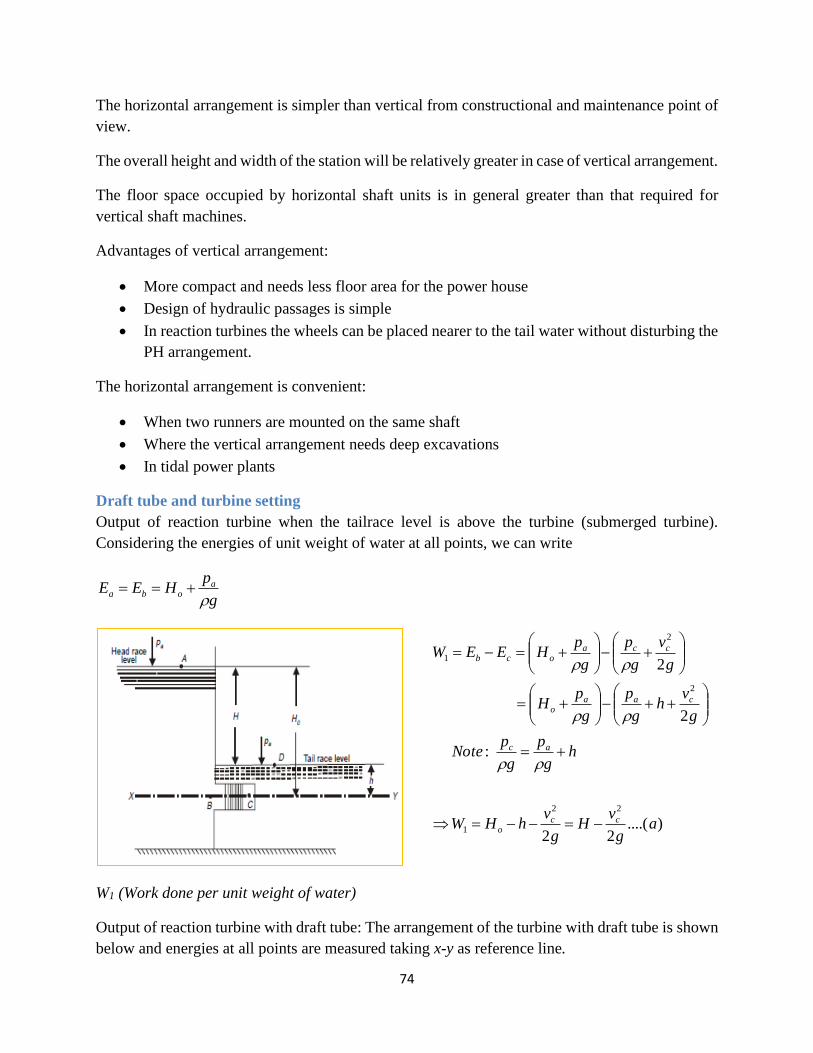
74
The horizontal arrangement is simpler than vertical from constructional and maintenance point of
view.
The overall height and width of the station will be relatively greater in case of vertical arrangement.
The floor space occupied by horizontal shaft units is in general greater than that required for
vertical shaft machines.
Advantages of vertical arrangement:
• More compact and needs less floor area for the power house
• Design of hydraulic passages is simple
• In reaction turbines the wheels can be placed nearer to the tail water without disturbing the
PH arrangement.
The horizontal arrangement is convenient:
• When two runners are mounted on the same shaft
• Where the vertical arrangement needs deep excavations
• In tidal power plants
Draft tube and turbine setting
Output of reaction turbine when the tailrace level is above the turbine (submerged turbine).
Considering the energies of unit weight of water at all points, we can write
g
pHEE a
oba
+==
)....(22
:
2
2
22
1
2
2
1
ag
vH
g
vhHW
hg
p
g
pNote
g
vh
g
p
g
pH
g
v
g
p
g
pHEEW
cco
ac
caao
ccaocb
−=−−=
+=
++−
+=
+−
+=−=
W1 (Work done per unit weight of water)
Output of reaction turbine with draft tube: The arrangement of the turbine with draft tube is shown
below and energies at all points are measured taking x-y as reference line.
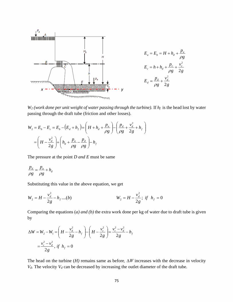
75
g
v
g
pE
g
v
g
phhE
g
phHEE
ddd
ccdc
adba
2
2
2
2
+=
+++=
++==
W2 (work done per unit weight of water passing through the turbine). If hf is the head lost by water
passing through the draft tube (friction and other losses).
( )
fda
dd
fdda
dfdbcb
hg
p
g
ph
g
vH
hg
v
g
p
g
phHhEEEEW
−
−++
−=
++−
++=+−=−=
2
2
2
2
2
The pressure at the point D and E must be same
dad hg
p
g
p+=
Substituting this value in the above equation, we get
0;2
)....(2
2
2
2
2 =−=−−= f
d
f
d hifg
vHWbh
g
vHW
Comparing the equations (a) and (b) the extra work done per kg of water due to draft tube is given
by
0,2
222
22
2222
12
=−
=
−−
=
−−
−−=−=
fdc
fdcc
fd
hifg
vv
hg
vv
g
vHh
g
vHWWW
The head on the turbine (H) remains same as before, ∆W increases with the decrease in velocity
Vd. The velocity Vd can be decreased by increasing the outlet diameter of the draft tube.
x y
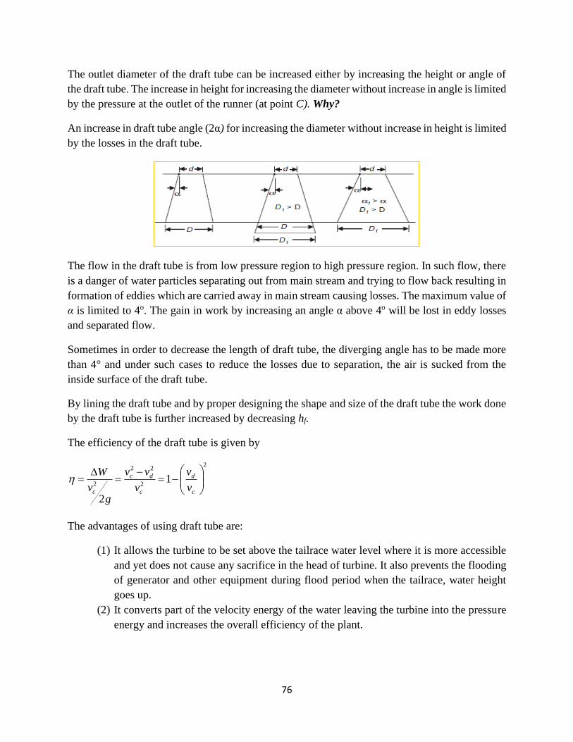
76
The outlet diameter of the draft tube can be increased either by increasing the height or angle of
the draft tube. The increase in height for increasing the diameter without increase in angle is limited
by the pressure at the outlet of the runner (at point C). Why?
An increase in draft tube angle (2α) for increasing the diameter without increase in height is limited
by the losses in the draft tube.
The flow in the draft tube is from low pressure region to high pressure region. In such flow, there
is a danger of water particles separating out from main stream and trying to flow back resulting in
formation of eddies which are carried away in main stream causing losses. The maximum value of
α is limited to 4o. The gain in work by increasing an angle α above 4o will be lost in eddy losses
and separated flow.
Sometimes in order to decrease the length of draft tube, the diverging angle has to be made more
than 4° and under such cases to reduce the losses due to separation, the air is sucked from the
inside surface of the draft tube.
By lining the draft tube and by proper designing the shape and size of the draft tube the work done
by the draft tube is further increased by decreasing hf.
The efficiency of the draft tube is given by
2
2
22
21
2
−=
−=
=
c
d
c
dc
c v
v
v
vv
gv
W
The advantages of using draft tube are:
(1) It allows the turbine to be set above the tailrace water level where it is more accessible
and yet does not cause any sacrifice in the head of turbine. It also prevents the flooding
of generator and other equipment during flood period when the tailrace, water height
goes up.
(2) It converts part of the velocity energy of the water leaving the turbine into the pressure
energy and increases the overall efficiency of the plant.
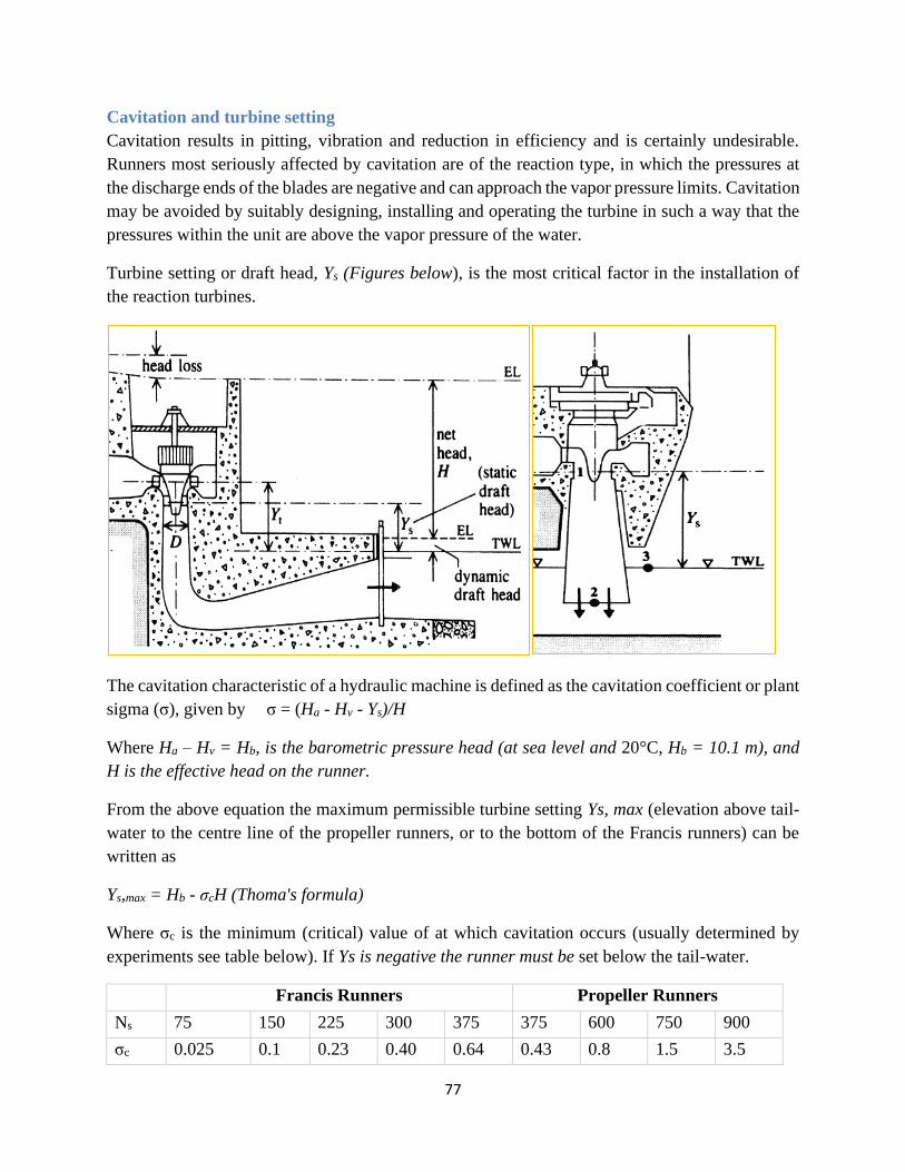
77
Cavitation and turbine setting
Cavitation results in pitting, vibration and reduction in efficiency and is certainly undesirable.
Runners most seriously affected by cavitation are of the reaction type, in which the pressures at
the discharge ends of the blades are negative and can approach the vapor pressure limits. Cavitation
may be avoided by suitably designing, installing and operating the turbine in such a way that the
pressures within the unit are above the vapor pressure of the water.
Turbine setting or draft head, Ys (Figures below), is the most critical factor in the installation of
the reaction turbines.
The cavitation characteristic of a hydraulic machine is defined as the cavitation coefficient or plant
sigma (σ), given by σ = (Ha - Hv - Ys)/H
Where Ha – Hv = Hb, is the barometric pressure head (at sea level and 20°C, Hb = 10.1 m), and
H is the effective head on the runner.
From the above equation the maximum permissible turbine setting Ys, max (elevation above tail-
water to the centre line of the propeller runners, or to the bottom of the Francis runners) can be
written as
Ys,max = Hb - σcH (Thoma's formula)
Where σc is the minimum (critical) value of at which cavitation occurs (usually determined by
experiments see table below). If Ys is negative the runner must be set below the tail-water.
Francis Runners Propeller Runners
Ns 75 150 225 300 375 375 600 750 900
σc 0.025 0.1 0.23 0.40 0.64 0.43 0.8 1.5 3.5

78
The above recommended limiting values of plant sigma (σc) may also be approximated by
• σc = 0.0432(Ns/100)2 for Francis runners
• σc = 0.28 + 0.0024(Ns/100)3 for propeller runners
• With an increase of σc by 10% for Kaplan turbines (Mosonyi, 1987).
The preliminary calculations of the elevation of the distributor above the tail water level (Yt, Fig.
above) suggest the following empirical relationships (Doland, 1957):
• Yt = Ys + 0.025DNs0.34 for Francis runners
• Yt = Ys + 0.41D for propeller runners
• Where D is the nominal diameter of the runner.
79
Chapter 5 Pressure Control and Speed Regulation Contents
1. Water Hammer theory and Analysis
2. Pressure Control Systems
3. Speed Terminology
4. Speed Control and Governors
5.1. Water hammer theory and analysis
Sudden shutdowns of hydroelectric plants or changes in water flow through hydraulic turbines
may cause problems ranging from rupture of penstocks due to water hammer to runner speed
changes that cause the line current of the generators to vary from the desired frequency.
Regulating the water flow and coping with sudden closure of gates and valves require special
equipment such as governors, pressure relief valves, and surge tanks. Solving the problems of
pressure control and speed regulation requires a thorough understanding of the basic theory of
water hammer.
Let us consider a simple case of fluid flowing with a certain velocity and brought to rest by closing
a valve at the downstream end. If the fluid is entirely incompressible and the wall of the pipe is
perfectly rigid, then all the fluid particles would have come to rest instantaneously. However, fluids
are compressible to a certain extent, thus particles will not decelerate uniformly. Only those
particles adjacent to the valve would stop instantaneously; other particles will come to rest later.
Recall Newton's second law: F = m (dv/dt); the more rapid the deceleration the greater would be
the force.
Water hammer is a phenomenon of pressure change in closed pipes caused when flowing water in
a pipeline is decelerated or accelerated by closing or opening a valve or changing the velocity of
the water rapidly in some other manner. The phenomenon is accompanied by a series of positive
and negative pressure waves which travel back and forth in the pipe system until they are damped
out by friction.
When a valve in a pipe or penstock carrying water is closed, the pressure head immediately
upstream of the valve is increased, and a pulse of high pressure is propagated upstream to the
nearest open water surface. On the downstream side of the valve a lowered pressure moves in a
downstream direction to the nearest open water surface. Flow is changing from one steady-state
to another over a very, very short time.
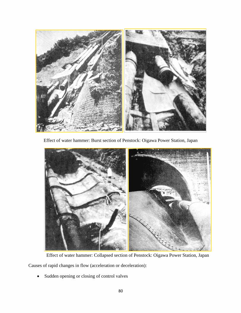
80
Effect of water hammer: Burst section of Penstock: Oigawa Power Station, Japan
Effect of water hammer: Collapsed section of Penstock: Oigawa Power Station, Japan
Causes of rapid changes in flow (acceleration or deceleration):
• Sudden opening or closing of control valves
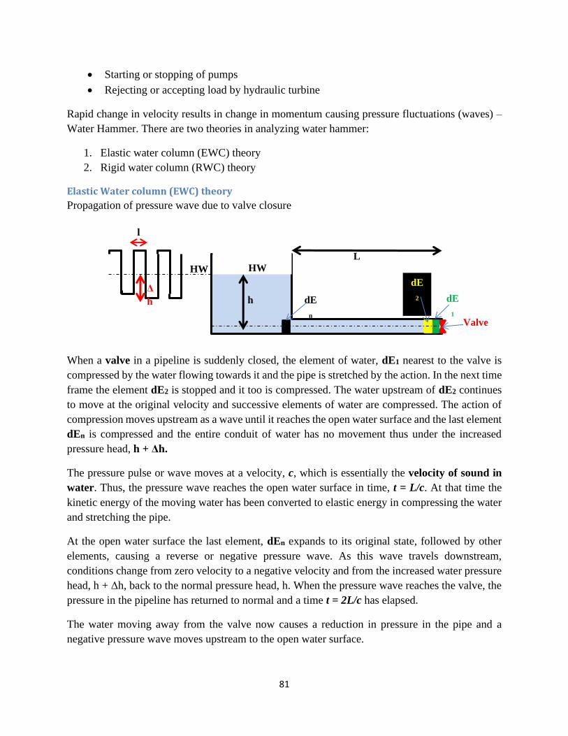
81
• Starting or stopping of pumps
• Rejecting or accepting load by hydraulic turbine
Rapid change in velocity results in change in momentum causing pressure fluctuations (waves) –
Water Hammer. There are two theories in analyzing water hammer:
1. Elastic water column (EWC) theory
2. Rigid water column (RWC) theory
Elastic Water column (EWC) theory
Propagation of pressure wave due to valve closure
When a valve in a pipeline is suddenly closed, the element of water, dE1 nearest to the valve is
compressed by the water flowing towards it and the pipe is stretched by the action. In the next time
frame the element dE2 is stopped and it too is compressed. The water upstream of dE2 continues
to move at the original velocity and successive elements of water are compressed. The action of
compression moves upstream as a wave until it reaches the open water surface and the last element
dEn is compressed and the entire conduit of water has no movement thus under the increased
pressure head, h + Δh.
The pressure pulse or wave moves at a velocity, c, which is essentially the velocity of sound in
water. Thus, the pressure wave reaches the open water surface in time, t = L/c. At that time the
kinetic energy of the moving water has been converted to elastic energy in compressing the water
and stretching the pipe.
At the open water surface the last element, dEn expands to its original state, followed by other
elements, causing a reverse or negative pressure wave. As this wave travels downstream,
conditions change from zero velocity to a negative velocity and from the increased water pressure
head, h + Δh, back to the normal pressure head, h. When the pressure wave reaches the valve, the
pressure in the pipeline has returned to normal and a time t = 2L/c has elapsed.
The water moving away from the valve now causes a reduction in pressure in the pipe and a
negative pressure wave moves upstream to the open water surface.
dE
1
dE
n
dE
2
Valve
L
h
HW
Δ
h
l
HW
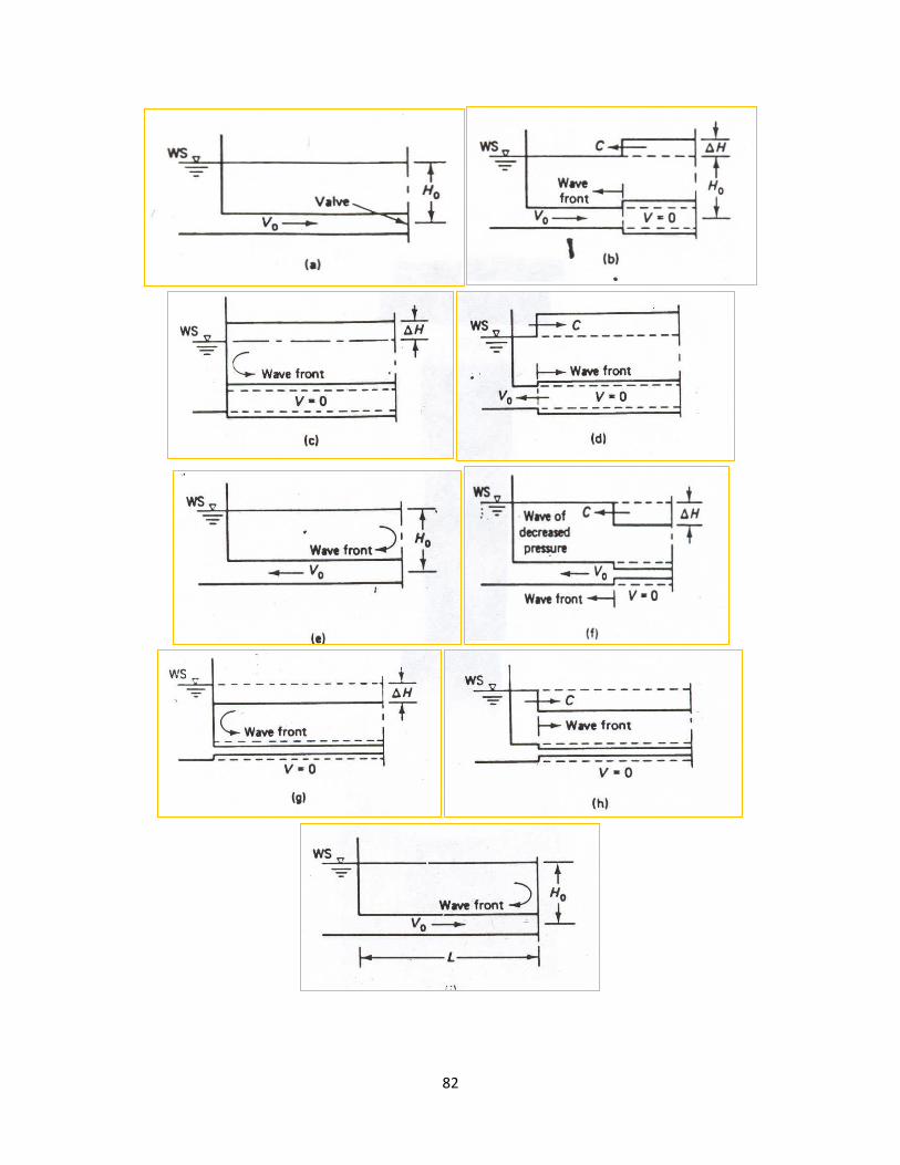
82
83
a. Steady state prior to valve closure
b. Rapid valve closure – pressure increase, pipe walls expand, liquid compression; transient
conditions propagate upstream
c. End of step 1 transient process @ L/c time
d. Pipe pressure > tank pressure water flows from pipe to tank relieving pressure in pipe
e. Process starts at tank and continues to valve; time L/c, [total time 2L/c → water hammer
period]
f. Wave of backwater cannot go past the valve, starts wave of negative pressure toward tank
g & h. Pressure difference causes water to flow toward valve
i. One full cycle, 4L/c (the original steady state condition fig a)
Pressure variation at the valve: velocity head and friction loss neglected would look like:
This periodic fluctuation at the reservoir
water level look like figure A, if the water did
not have friction acting. In reality, friction
does act within the water and at the
boundaries so that the pulses of pressure
change have decreasing amplitude as shown
in Figure B.
Water hammer pressure is a function of
… ?
Dh
Pre
ssure
hea
d
Time
Reservoir level
c
L4
c
L8
c
L12
84
Process Considerations
• Pressure wave, resulting from compression of water, travels at speed of sound (sonic) in
water
• Pressure change due to change in velocity
• Pressure increase moderated by expansion of the pipe wall due to increase in pressure
Pipe Support Conditions
1. Pipe supported at one end, pipe is allowed to move and pressure increase generates both
axial and lateral stresses
2. Pipe anchored against axial movement throughout, no axial movement but axial stress still
generated
3. No axial movement plus expansion joints at regular intervals, axial stress is taken up by
play in joints
Theory & terms
Δh = increase in head relative to original head (assume frictionless flow)
Assume vo is actual velocity in pipe based on friction, steady state prior to valve closure. Increase
in pressure due to water hammer must be added to the steady-state pressure prevailing just before
valve closure.
To find c (speed of pressure wave) we need to relate the volume of water entering the pipe to the
increased pipe volume due to pipe expansion and the reduced volume of water because of
compression. This approach needs the following parameters
• E = modulus of elasticity of pipe material
• K = bulk modulus of elasticity of fluid
• c = speed of pressure wave, celerity
• Δh = increase in pressure head above initial conditions
According to Parmakian (1955), the velocity of the pressure wave, c, in a pipe is given by the
following formula:
5.0
11−
+=
tE
dC
Kc
Where ρ = density of the water; K =volume modulus of water; d = diameter of pipe; t = thickness
of pipe; E = pipe’s Young's modulus of elasticity; C1 = factor for anchorage and support of pipe
• C1 = 0.95 for pipe anchored at upper end and without expansion joints
• C1 = 0.91 for pipe anchored against longitudinal movement
• C1 = 0.85 for pipe with expansion joints.
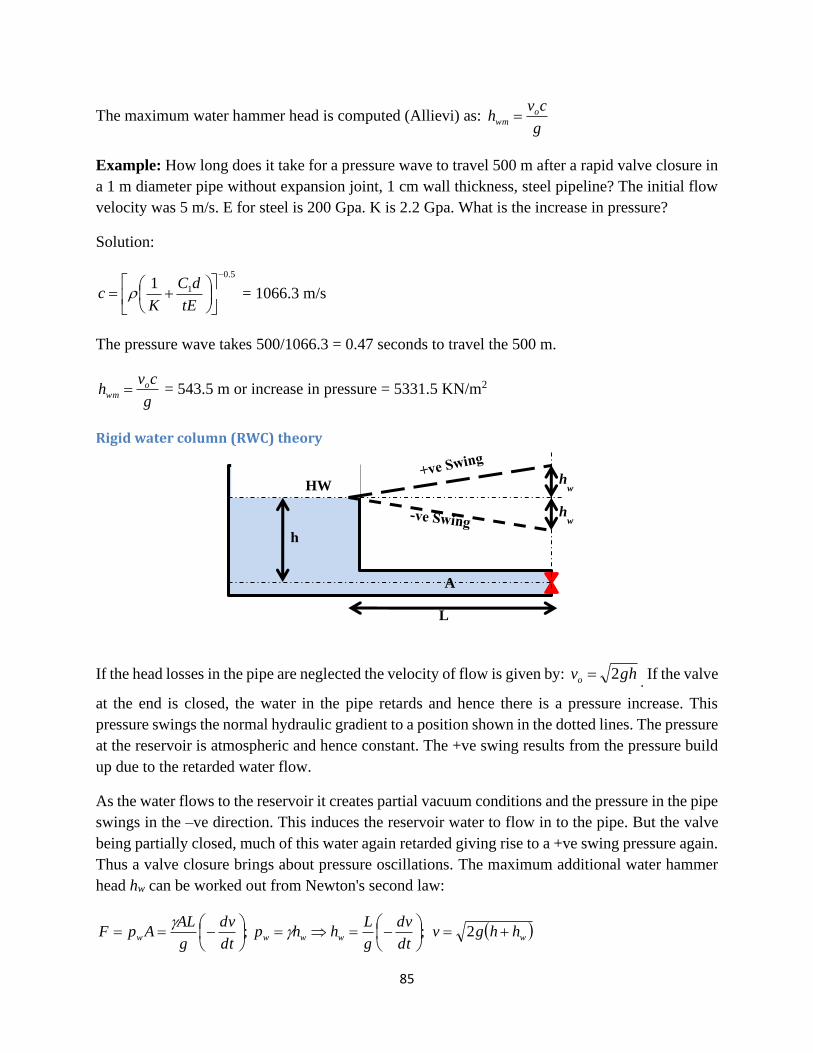
85
The maximum water hammer head is computed (Allievi) as: g
cvh o
wm =
Example: How long does it take for a pressure wave to travel 500 m after a rapid valve closure in
a 1 m diameter pipe without expansion joint, 1 cm wall thickness, steel pipeline? The initial flow
velocity was 5 m/s. E for steel is 200 Gpa. K is 2.2 Gpa. What is the increase in pressure?
Solution:
5.0
11−
+=
tE
dC
Kc = 1066.3 m/s
The pressure wave takes 500/1066.3 = 0.47 seconds to travel the 500 m.
g
cvh o
wm = = 543.5 m or increase in pressure = 5331.5 KN/m2
Rigid water column (RWC) theory
If the head losses in the pipe are neglected the velocity of flow is given by: ghvo 2=. If the valve
at the end is closed, the water in the pipe retards and hence there is a pressure increase. This
pressure swings the normal hydraulic gradient to a position shown in the dotted lines. The pressure
at the reservoir is atmospheric and hence constant. The +ve swing results from the pressure build
up due to the retarded water flow.
As the water flows to the reservoir it creates partial vacuum conditions and the pressure in the pipe
swings in the –ve direction. This induces the reservoir water to flow in to the pipe. But the valve
being partially closed, much of this water again retarded giving rise to a +ve swing pressure again.
Thus a valve closure brings about pressure oscillations. The maximum additional water hammer
head hw can be worked out from Newton's second law:
( )wwwww hhgvdt
dv
g
Lhhp
dt
dv
g
ALApF +=
−==
−== 2;;
L
h
HW hw
hw
A
86
5.2. Pressure control systems
Hydraulic transients and pressure changes such as water hammer can be controlled in several ways.
Gate controls and governor regulation can limit the gate or valve closure time so that there is no
damaging pressure head rise. Pressure regulator valves located near the turbine can be used. The
relief valve can be connected to the turbine spiral case and controlled by the turbine gate
mechanism to prevent excessive pressure by maintaining a nearly constant water velocity in the
penstock. The relief valve may be designed to close at a rate which limits pressure rise to an
acceptable value.
Design considerations
• Specify a slow closure time
• Safety factor by doubling the minimum closure time
• Automatic valves programmed to prevent rapid closure
• Surge tanks
Valve Closure rate
Rapid Valve Closure means the time of closure c
Ltc
2 and full water hammer pressure is
developed. o
o cvporg
cvh == ,
Full pressure wave will not develop, if c
Lt
c
Lc
202 and the estimated water hammer head would
be c
o
estt
cL
g
cvh
2
=
Slow Closure after Lorenzo & Allievi will develop a pressure:
( )
=++=co
oo tp
LvNwhereNNNpp
,25.05.0 2
Surge Tanks
Another way of pressure control can be accomplished with surge tanks. Surge tanks are vertical
standpipes that act as a Forebay and shorten the distance for relief from the pressure wave of water
hammer. A surge tank serves a threefold purpose:
1. Flow stabilization to the turbine,
2. Water hammer relief or pressure regulation, and
3. Improvement of speed control.
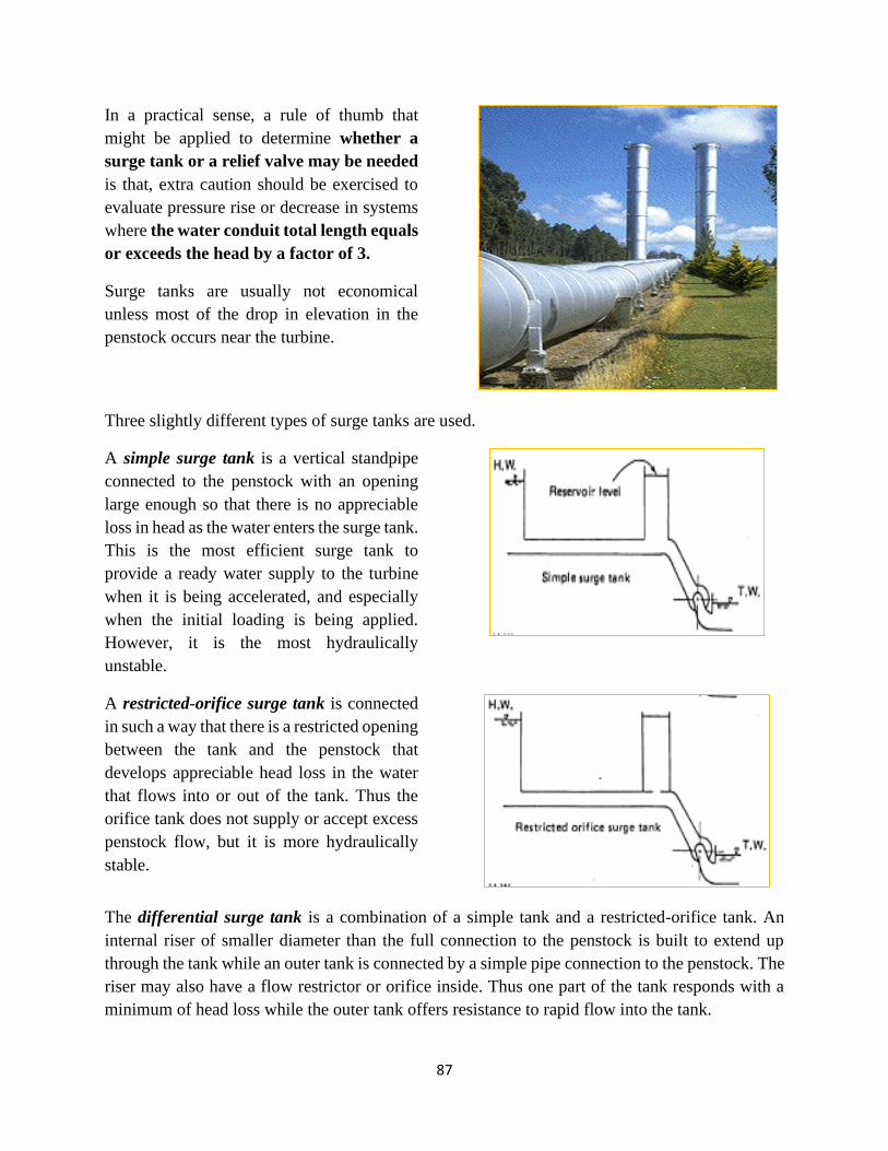
87
In a practical sense, a rule of thumb that
might be applied to determine whether a
surge tank or a relief valve may be needed
is that, extra caution should be exercised to
evaluate pressure rise or decrease in systems
where the water conduit total length equals
or exceeds the head by a factor of 3.
Surge tanks are usually not economical
unless most of the drop in elevation in the
penstock occurs near the turbine.
Three slightly different types of surge tanks are used.
A simple surge tank is a vertical standpipe
connected to the penstock with an opening
large enough so that there is no appreciable
loss in head as the water enters the surge tank.
This is the most efficient surge tank to
provide a ready water supply to the turbine
when it is being accelerated, and especially
when the initial loading is being applied.
However, it is the most hydraulically
unstable.
A restricted-orifice surge tank is connected
in such a way that there is a restricted opening
between the tank and the penstock that
develops appreciable head loss in the water
that flows into or out of the tank. Thus the
orifice tank does not supply or accept excess
penstock flow, but it is more hydraulically
stable.
The differential surge tank is a combination of a simple tank and a restricted-orifice tank. An
internal riser of smaller diameter than the full connection to the penstock is built to extend up
through the tank while an outer tank is connected by a simple pipe connection to the penstock. The
riser may also have a flow restrictor or orifice inside. Thus one part of the tank responds with a
minimum of head loss while the outer tank offers resistance to rapid flow into the tank.
88
Hydraulic design of simple surge tank
Applying continuity equation: Q = As x (dz/dt) + Q1; Q = vtAt
dz/dt = (vtAt – Q1)/As … (Eq. 1)
Where At and As are the x-sectional area of the tunnel and surge tank
At steady state the water level in the surge tank will be at –z = zo
Applying Energy Equation: g
v
D
Lfz t
o2
2
=
2.....2
;0
2
2Eq
gD
LfFWhere
A
A
dt
dv
g
LzvF t
s
tt
tt ==
++−
If throated head loss in the throat is also considered:
0
2
22=
++−−
s
tsStt
A
A
dt
dv
g
LzvFvF
Q
Q1
zo
L
+z
D = diameter
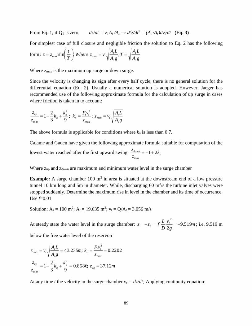
89
From Eq. 1, if Q1 is zero, dz/dt = vt At /As → d2z/dt2 = (At /As)dvt/dt (Eq. 3)
For simplest case of full closure and negligible friction the solution to Eq. 2 has the following
form: gA
LAT
gA
LAvzWhere
T
tzz
s
t
s
tt ==
= ;;sin maxmax
Where zmax is the maximum up surge or down surge.
Since the velocity is changing its sign after every half cycle, there is no general solution for the
differential equation (Eq. 2). Usually a numerical solution is adopted. However; Jaeger has
recommended use of the following approximate formula for the calculation of up surge in cases
where friction is taken in to account:
gA
LAvz
z
vFk
kk
z
z
s
tt
tto
oo
up==+−= max
max
22
max
;;93
21
The above formula is applicable for conditions where ko is less than 0.7.
Calame and Gaden have given the following approximate formula suitable for computation of the
lowest water reached after the first upward swing: odown k
z
z21
max
+−=
Where zup and zdown are maximum and minimum water level in the surge chamber
Example: A surge chamber 100 m2 in area is situated at the downstream end of a low pressure
tunnel 10 km long and 5m in diameter. While, discharging 60 m3/s the turbine inlet valves were
stopped suddenly. Determine the maximum rise in level in the chamber and its time of occurrence.
Use f=0.01
Solution: As = 100 m2; At = 19.635 m2; vt = Q/At = 3.056 m/s
At steady state the water level in the surge chamber: mg
v
D
Lfzz t
o 519.92
2
−==−= ; i.e. 9.519 m
below the free water level of the reservoir
mzk
kz
z
z
vFkm
gA
LAvz
upo
o
up
tto
s
tt
12.37;8586.093
21
2202.0;235.43
2
max
max
2
max
==+−=
====
At any time t the velocity in the surge chamber vs = dz/dt; Applying continuity equation:
90
sec732.7712.37;519.96.0
519.9519.90;6.06.0
6.0;0; 11
==−=
−=−==+===
===+=
tmzforthustz
mcmztatctzdt
dzv
vQButQQvAAv
s
ssstt
5.3. Speed terminology
A speed term that is important in the safety of hydropower plants is the runaway speed. It is the
speed attained by turbine and generator (if directly connected)
• After a load rejection,
• If for some reason the shutdown mechanism fails to shut down the unit or
• If the rate of shutdown is not fast enough.
Runaway speed may reach 170 to 300% of normal operating speed. The magnitude of runaway
speed is related to turbine design, operation, and setting of the turbine and will vary with the
windage and friction that the runner and generator rotor offer as a revolving mass.
For some adjustable blade propeller turbines, the maximum runaway speed may be as high as
300% of normal operating speed.
Accurate numbers for defining runaway speed values must be based on model tests conducted by
the turbine manufacturers.
Type of runner Runaway speed (% of normal
speed)
Acceptable head Variation
Minimum Maximum
Impulse 170-190 65 125
Francis 200-220 50 150
Propeller 250-300 50 150
The U.S. Department of the Interior (1976) gives empirical equations for estimating runaway speed
based on several model tests of units installed by the Bureau of Reclamation. The equations are:
dr
sssr
hh
nn
unitsmetricinnNnnnn
maxmax
2.02.0 63.0;85.0
=
==
Where
• nr = runaway speed at best
efficiency head and full gate, rpm;
• n = normal rotational speed, rpm;
• nmax= runaway speed at maximum
head;
• ns = specific speed based on full
gate output at best efficiency head;
• hd = design head;
• hmax = maximum head.

91
Another term is over-speed. It is the speed attained under transient conditions by a turbine after
load rejection, while the governing and gate closure mechanisms are going into action. The rapidity
with which the shutoff operates controls how much the over-speed will be? In very slow moving
gate mechanisms over-speed can approach runaway speed.
5.4. Speed control and governors
Regulating the quantity of water admitted to the turbine runner is the usual means of regulating
and maintaining a constant speed to drive the generator and to regulate the power output. This is
done by operating wicket gates or valves. Such action requires a mechanism to control the wicket
gates, which is the governor or governor system.
The function of the governor is to detect any error in speed between actual and desired values and
to effect a change in the turbine output. This is done so that the system load is in equilibrium with
the generating unit output at the desired speed.
The function of the governor is to keep the speed of the prime mover constant irrespective of load
variation. The governor is then controls the amount of water flowing through the turbine. Since
the governor has to deal with water coming at very large force and in huge quantity, it should be
very strong. To achieve this all types of turbines, use oil pressure governor.
Speed droop
If two or more generating units are operating to govern a system, it is impossible for them to
maintain exactly the same speed. The governor with the higher speed will try to bring the system
up to its speed, and take on load until it either achieves this or the turbine reaches full-gate position.
If it is able to raise the system frequency, the other governor will sense too high speed and begin
to drop load. The governors will therefore oppose each other. To avoid this situation, governors
are built with a feature called speed droop.
Speed droop reduces the governor sensing speed as the gate opening or load increases. It is defined
as the difference in speed (in percent) permitted when the units are operating between zero gate
opening and 100% gate opening.
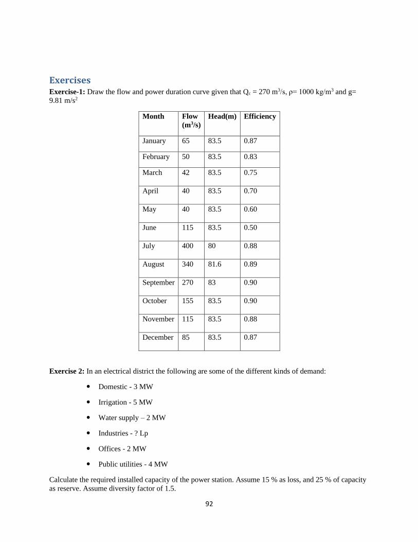
92
Exercises Exercise-1: Draw the flow and power duration curve given that Qc = 270 m3/s, ρ= 1000 kg/m3 and g=
9.81 m/s2
Month Flow
(m3/s)
Head(m) Efficiency
January 65 83.5 0.87
February 50 83.5 0.83
March 42 83.5 0.75
April 40 83.5 0.70
May 40 83.5 0.60
June 115 83.5 0.50
July 400 80 0.88
August 340 81.6 0.89
September 270 83 0.90
October 155 83.5 0.90
November 115 83.5 0.88
December 85 83.5 0.87
Exercise 2: In an electrical district the following are some of the different kinds of demand:
Domestic - 3 MW
Irrigation - 5 MW
Water supply – 2 MW
Industries - ? Lp
Offices - 2 MW
Public utilities - 4 MW
Calculate the required installed capacity of the power station. Assume 15 % as loss, and 25 % of capacity
as reserve. Assume diversity factor of 1.5.

93
Exercise 3: When a run-of-river plant operates as a peak load station with a weekly load factor of 20%,
all its capacity is firm capacity. What will be the minimum flow in the river so that the station may serve
as the base load station? It is given that
Rated installed capacity of generator = 10 MW
Operating head = 15 m
Plant efficiency = 80%
Estimate the daily load factor of the plant if the stream flow is 15 m3/s.
Exercise 4: A common load is shared by two stations, one being a base load plant with 25 MW installed
capacity and other being a standby station with 30 MW capacity. The yearly output of the standby station
is 10.5 x 10⁶ kWh and that of the base load plant is 125 x 106 kWh. The peak load taken by the standby
station is 15 MW and this station works for 2500 hours during the year. The base load station takes a peak
of 22.5 MW. Find out:
(i) Annual load factor for both stations;
(ii) Capacity factor for both stations.
Exercise 5: The available flow for 97% of the time (i.e., in a year) in a river is 30 m3/s. A run-of-river
plant is proposed on this river to operate for 6 days in a week round the clock. The plant supplies power to
a variable load whose variation is given below:
(v) Pondage required
Exercise 6: The average weekly discharge as measured at a given site is as follows:

94
(a) Plot
(i) The hydrograph of weekly flow.
(ii) The flow-duration curve.
(iii) The power-duration curve if the head available is 50 m and the efficiency of the plant set is
85%.
(b) Determine the power that can be developed per m3, the maximum power, average power, and total
energy produced during 26 weeks.
Exercise 6: Average daily flows in a river in a typical low water week are given below. A run-of-river
hydropower plant is proposed on this river to operate 6 days in a week round the clock. The full pond
effective head on turbines is 20 m and the plant efficiency is 80%. Maximum allowable fluctuation of
pond level is 1 m.
Determine:
(i) the capacity of the pond required to give a maximum uniform output;
(ii) the weekly energy output (kWh) from the plant.
Day Su Mo Tu We Th Fr Sa
Flow (m3/s) 26 35 40 50 45 40 30
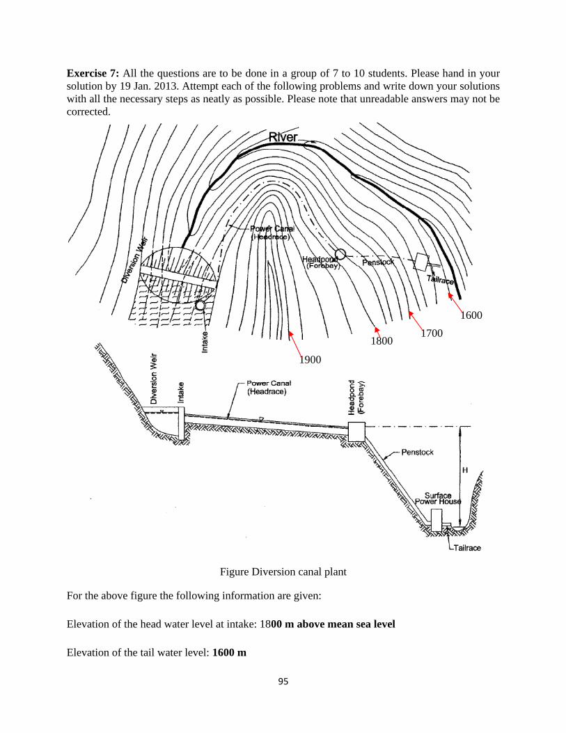
95
Exercise 7: All the questions are to be done in a group of 7 to 10 students. Please hand in your
solution by 19 Jan. 2013. Attempt each of the following problems and write down your solutions
with all the necessary steps as neatly as possible. Please note that unreadable answers may not be
corrected.
Figure Diversion canal plant
For the above figure the following information are given:
Elevation of the head water level at intake: 1800 m above mean sea level
Elevation of the tail water level: 1600 m
1800 1700
1600
1900
96
Length of the power canal: 5000 m
The power canal traverses in high seepage geological setting.
Steel Penstock Length = 200 m;
Coefficient of friction f for the penstock = 0.02.
The maximum discharge to be diverted from the head water for 14 hour power production is 30
m3/s.
Overall efficiency (ɳt): 80%
Generator: frequency = 60 Hz; Number of poles = 24.
Turbine type to be used: reaction turbine.
Unit weight of water = 9.81 KN/m3
Barometric head = 10.3 m
Assume any other value if necessary.
1. Design the power canal
2. The Forebay storage capacity (if needed)
3. Decide on the number of Penstocks, diameter and thickness
4. Determine the maximum power output from the installation
5. Decide on the type of reaction turbine.
6. Decide on the number and capacity of reaction turbines for the installation.
7. Design a scroll casing for the turbine.
8. Determine the safe turbine setting relative to the tail water level
9. If a simple surge chamber 5 m in diameter is provided at 50 m from the Forebay determine
the maximum up surge and down surge in the surge chamber for sudden rejection by the
turbine.
10. Comment on using the Forebay as a surge chamber or vice versa
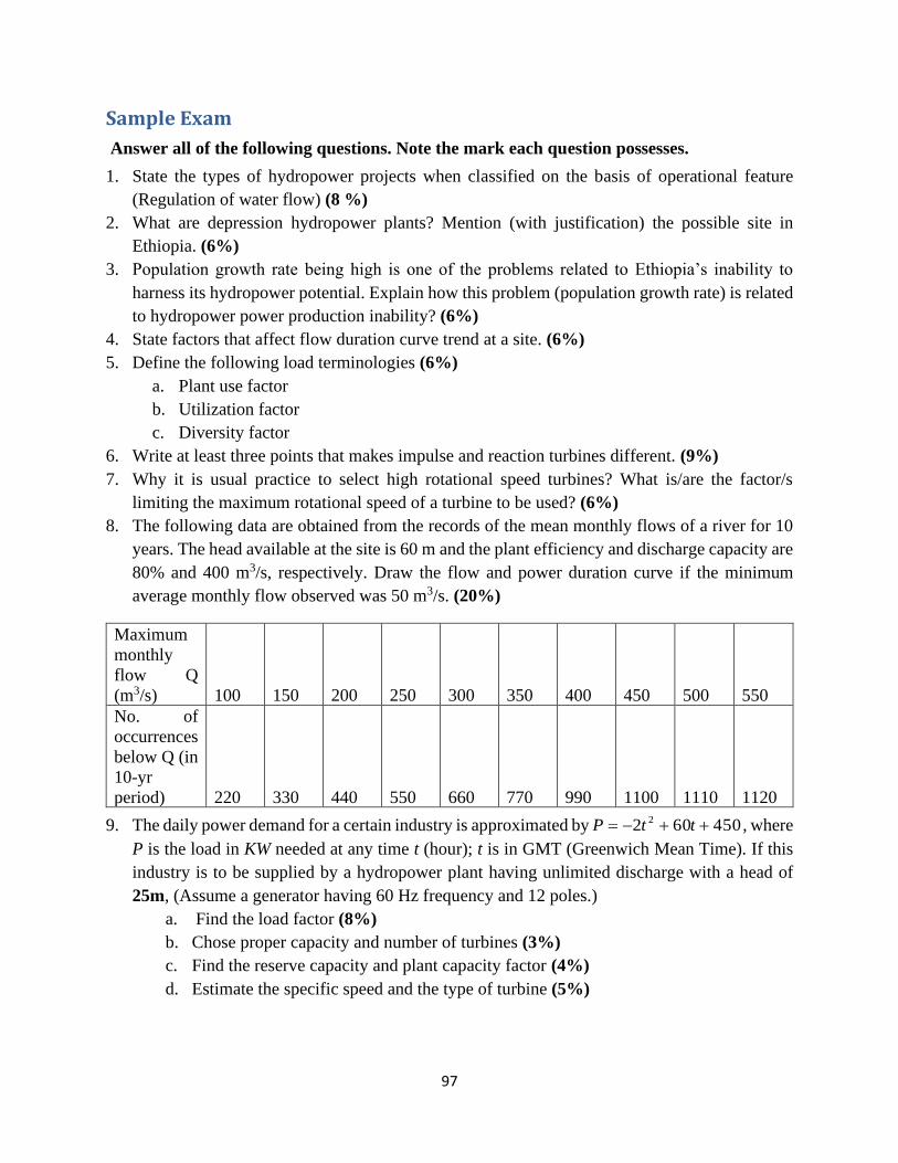
97
Sample Exam
Answer all of the following questions. Note the mark each question possesses.
1. State the types of hydropower projects when classified on the basis of operational feature
(Regulation of water flow) (8 %)
2. What are depression hydropower plants? Mention (with justification) the possible site in
Ethiopia. (6%)
3. Population growth rate being high is one of the problems related to Ethiopia’s inability to
harness its hydropower potential. Explain how this problem (population growth rate) is related
to hydropower power production inability? (6%)
4. State factors that affect flow duration curve trend at a site. (6%)
5. Define the following load terminologies (6%)
a. Plant use factor
b. Utilization factor
c. Diversity factor
6. Write at least three points that makes impulse and reaction turbines different. (9%)
7. Why it is usual practice to select high rotational speed turbines? What is/are the factor/s
limiting the maximum rotational speed of a turbine to be used? (6%)
8. The following data are obtained from the records of the mean monthly flows of a river for 10
years. The head available at the site is 60 m and the plant efficiency and discharge capacity are
80% and 400 m3/s, respectively. Draw the flow and power duration curve if the minimum
average monthly flow observed was 50 m3/s. (20%)
Maximum
monthly
flow Q
(m3/s) 100 150 200 250 300 350 400 450 500 550
No. of
occurrences
below Q (in
10-yr
period) 220 330 440 550 660 770 990 1100 1110 1120
9. The daily power demand for a certain industry is approximated by 450602 2 ++−= ttP , where
P is the load in KW needed at any time t (hour); t is in GMT (Greenwich Mean Time). If this
industry is to be supplied by a hydropower plant having unlimited discharge with a head of
25m, (Assume a generator having 60 Hz frequency and 12 poles.)
a. Find the load factor (8%)
b. Chose proper capacity and number of turbines (3%)
c. Find the reserve capacity and plant capacity factor (4%)
d. Estimate the specific speed and the type of turbine (5%)
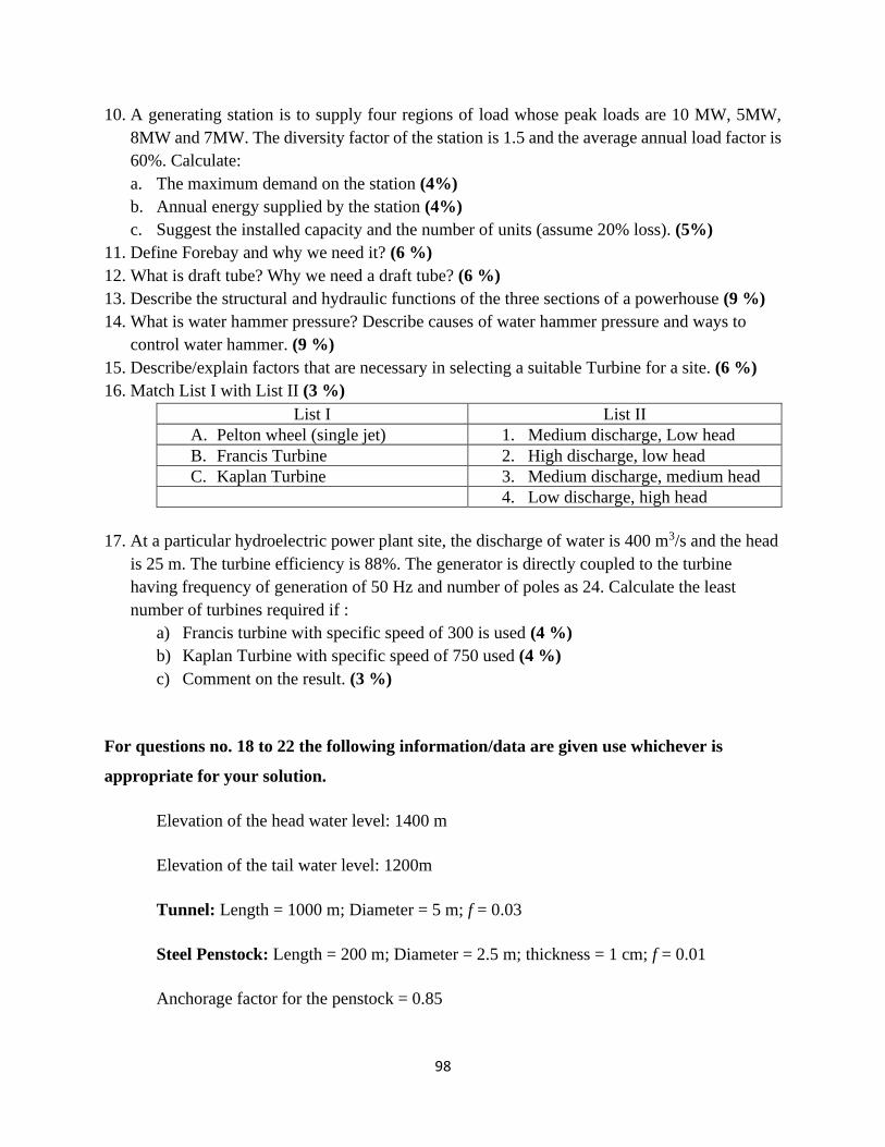
98
10. A generating station is to supply four regions of load whose peak loads are 10 MW, 5MW,
8MW and 7MW. The diversity factor of the station is 1.5 and the average annual load factor is
60%. Calculate:
a. The maximum demand on the station (4%)
b. Annual energy supplied by the station (4%)
c. Suggest the installed capacity and the number of units (assume 20% loss). (5%)
11. Define Forebay and why we need it? (6 %)
12. What is draft tube? Why we need a draft tube? (6 %)
13. Describe the structural and hydraulic functions of the three sections of a powerhouse (9 %)
14. What is water hammer pressure? Describe causes of water hammer pressure and ways to
control water hammer. (9 %)
15. Describe/explain factors that are necessary in selecting a suitable Turbine for a site. (6 %)
16. Match List I with List II (3 %)
List I List II
A. Pelton wheel (single jet) 1. Medium discharge, Low head
B. Francis Turbine 2. High discharge, low head
C. Kaplan Turbine 3. Medium discharge, medium head
4. Low discharge, high head
17. At a particular hydroelectric power plant site, the discharge of water is 400 m3/s and the head
is 25 m. The turbine efficiency is 88%. The generator is directly coupled to the turbine
having frequency of generation of 50 Hz and number of poles as 24. Calculate the least
number of turbines required if :
a) Francis turbine with specific speed of 300 is used (4 %)
b) Kaplan Turbine with specific speed of 750 used (4 %)
c) Comment on the result. (3 %)
For questions no. 18 to 22 the following information/data are given use whichever is
appropriate for your solution.
Elevation of the head water level: 1400 m
Elevation of the tail water level: 1200m
Tunnel: Length = 1000 m; Diameter = 5 m; f = 0.03
Steel Penstock: Length = 200 m; Diameter = 2.5 m; thickness = 1 cm; f = 0.01
Anchorage factor for the penstock = 0.85
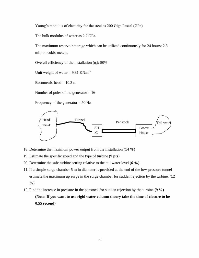
99
Young’s modulus of elasticity for the steel as 200 Giga Pascal (GPa)
The bulk modulus of water as 2.2 GPa.
The maximum reservoir storage which can be utilized continuously for 24 hours: 2.5
million cubic meters.
Overall efficiency of the installation (ɳt): 80%
Unit weight of water = 9.81 KN/m3
Borometric head = 10.3 m
Number of poles of the generator = 16
Frequency of the generator = 50 Hz
18. Determine the maximum power output from the installation (14 %)
19. Estimate the specific speed and the type of turbine (9 pts)
20. Determine the safe turbine setting relative to the tail water level (6 %)
11. If a simple surge chamber 5 m in diameter is provided at the end of the low-pressure tunnel
estimate the maximum up surge in the surge chamber for sudden rejection by the turbine. (12
%)
12. Find the increase in pressure in the penstock for sudden rejection by the turbine (9 %)
(Note: If you want to use rigid water column theory take the time of closure to be
0.55 second)
Tail water
SU
.C
H.
Power
House
Head
water
Tunnel Penstock