wireless sensor networks: communication mechanisms for power-aware
TRANSCRIPT

Wireless Sensor Networks: Communication Mechanisms for
Power-Aware Data Dissemination
Mario CagaljSwiss Federal Institute of Technology at Lausanne
EPFLSwitzerland
June, 2001

Abstract
A wireless sensor network is an ad hoc network consisting of numerous sensor devices (nodes).These nodes are linked via short-range ad hoc radio connections. Each node in such a networkhas a limited energy resource (battery), and each node operates unattended. Consequently,energy efficiency is an important design consideration for these networks. Inspired by thefact that in complex systems in nature each element follows simple rules in order to attain acommon goal, we design energy efficient routing mechanisms that mimic this concept. Theproposed unicast routing mechanism requires only local coordination of nodes to build aminimum cost topology (tree) on a network. Each node then uses power-aware selection toroute data along a minimum cost route towards the target node. The proposed broadcastmechanism minimizes the number of rebroadcasting nodes by exploiting the broadcast natureof the wireless channel. We show that a simple local scheme executed at each node sufficesto keep the number of retransmitting nodes close to a minimum number. Both communica-tion mechanisms take into account the nodes’ limited energy resources, and thus extend thelifetimes of the sensor nodes.
We evaluate the broadcast mechanism using simulation. We find that it exhibits goodscalability and power-aware characteristics.

Contents
Introduction 21.1 A General Operational Scenario . . . . . . . . . . . . . . . . . . . . . . . . . . 3
Models 52.1 Power Consumption Model . . . . . . . . . . . . . . . . . . . . . . . . . . . . 52.2 Network Model . . . . . . . . . . . . . . . . . . . . . . . . . . . . . . . . . . . 6
Power-aware Unicast Communication 83.1 Metric for Power-Aware Unicast Communication . . . . . . . . . . . . . . . . 83.2 Minimum Cost Topology . . . . . . . . . . . . . . . . . . . . . . . . . . . . . . 9
Power-aware Broadcast Communication 144.1 Broadcast Covering Problem (BCP) . . . . . . . . . . . . . . . . . . . . . . . 144.2 Metric for Power-Aware Broadcast Communication . . . . . . . . . . . . . . . 154.3 Distributed Heuristic Solution for the BCP . . . . . . . . . . . . . . . . . . . 164.4 Broadcast Simulations . . . . . . . . . . . . . . . . . . . . . . . . . . . . . . . 18
Conclusion 21
APPENDIX A . . . . . . . . . . . . . . . . . . . . . . . . . . . . . . . . . . . . . . 22APPENDIX B . . . . . . . . . . . . . . . . . . . . . . . . . . . . . . . . . . . . . . 23
1

Introduction
Recent advances in IC technology make it possible to produce inexpensive micro-sensingdevices that are equipped with processing, memory and wireless communication capabilities[1, 2]. Such sophisticated devices allow for the production of systems (networks) that linkthe physical world to cyberspace and thus introduce a new information flow: person toenvironment. The size and cost of the sensors enable applications to network thousands ofthese sensors in order to achieve high quality sensing of the environment. Such networkscan be rapidly deployed over any given area. Once the network is deployed, the sensornodes coordinate their activities to support all the sensing tasks required. Environmentalinformation gathered could be processed locally, or sent to data collection points. Wirelesssensor networks are likely to be widely used for environmental information gathering andprocessing.
Applications of wireless sensor networks include monitoring of inhospitable physical en-vironments (industrial zones, disaster zones, battlefields), environmental control in offices(smart offices), interactive environments (kindergartens, museums), and remote health care(BodyLAN, interfaces for disabled).
Application diversity can be greatly extended by providing a convenient way to remotelyaccess sensor data. One way to meet this goal is to achieve inter-operability between sen-sor networks and existing communication infrastructures (Internet, LAN, cellular networks,etc.). Such inter-operability between sensor networks and conventional networks demandsemployment of gateway or sink1 nodes. The sink nodes represent interfaces through whichmessages are exchanged between two networks. Information gathered from the environmentis available to a remote user at these sink nodes. A remote user sends its queries into thesensor network through the sink nodes.
The sensor nodes have limited energy resources that will be consumed for processingenvironmental information or for transmitting the information. Sending information, in thesekind of networks, with a single hop over a long distance, is characterized by high powertransmission. By contrast, use of multiple hops to reach a destination can result in lowerenergy consumption. Furthermore, using multiple hops, a sending node can also reach nodesthat are out of the transmission range of the sending node.
Our approach to energy efficient unicast communication is based on building a minimumcost topology (tree) on the multi-hop sensor networks. The sink node initiates tree building,that is it initiates routes from the sensor nodes in the network to itself. Each node choosesa minimum cost route to send data towards the sink node. For this purpose, we adaptedand used the concept of minimum power topology. In [3] the authors developed a generalmathematical theory for building a minimum power topology on a stationary network. Thekey idea behind their work is that energy efficient transmission can be achieved by eachnode when it considers only its immediate locality, that is, its closest neighbors. This result
1Throughout this report we also use the term sink to denote every node that initiates local coordination
2

obviously implies that the overall power consumption of such a network will be close tominimum one.
With regard to broadcast communication, our focus is on source-initiated broadcasting ofinformation. Information is distributed from the source node towards each node in a whole orpart of the sensor network. The main objective is to minimize the number of rebroadcastingnodes and still ensure that each node in the network is reached. In order to achieve this goalwe use the node-based multicast model, which was introduced by the authors in [4]. In thenode-base model there is a trade-off between reaching more nodes in a single hop by usinghigher power versus reaching fewer nodes using lower power. This trade-off is possible dueto the broadcast nature of wireless channel.
Our communication mechanisms put emphasis on the remaining battery capacity of thenodes. This is a crucial issue in the unattended wireless sensor networks. Taking into accountthe nodes’ remaining power we are able to evenly distribute the energy load among the sensorsin the network. The idea behind this approach is that all nodes in the network are equallyimportant, and that the nodes in the network remain up and running together for as long aspossible. In order to achieve this goal we use power-aware metrics.
Another crucial issue in these kind of networks is scalability, that is the influence of thenumber of nodes on the communication performance. Our approach to coping with thisproblem is based on the behavior of complex systems in nature, where each element followssimple rules in order to achieve a common goal. We design the communication mechanismsthat mimic this concept: each node in the network follows simple rules in order to disseminatedata throughout the network. With this approach our communication mechanisms exhibitgood scalability characteristic.
The key features of our communication mechanisms are:
• Localized coordination of the sensor nodes (scalability)
• Evenly distributed energy load
• Increased fault tolerance (multiple points of failure)
1.1 A General Operational Scenario
A typical application of the wireless sensor network includes numerous sensor nodes thatare scattered randomly over any given area. Each node is assumed to be equipped withprocessing, memory and wireless communication capabilities. Limited energy resources (bat-teries) allow each node to operate for some finite period (this period depends on employedcommunication protocols).
Once the sensor nodes have woken up, they begin to establish a wireless, multi-hopcommunication network. The sensor nodes begin to establish routes by which gatheredinformation is passed to one or more sink nodes. The sink node may have the same capabilitiesas other network nodes, or it may be equipped with long-range radio, with more memoryand processing power. However, the sink nodes have to enable the connection between thesensor network and existing communication infrastructure (Internet, cellular networks, etc.).
From our point of view there are three typical operational modes for accessing sensors’data.
On Demand Reply (ODR) - In the ODR mode the sensor nodes send information to thesink node in reply to a sink node query. Thus, the sensor nodes reply on demand. In this mode,
3

once a sensor node has replied to a query, it will not send further until a new query comes.From the moment the node has replied to the sink node, it keeps to collect an environmentalinformation and shares it with its neighbors to perform a distributed processing, increasingaccuracy of sensed data. This communication model is known as local cooperation. The datawhose quality exceeds some predefined threshold will be eventually aggregated at multiplenodes. With the same data stored at multiple nodes, the degree of protection against failureof nodes is increased.
The sink node interrogates the network for information by broadcasting queries of a ODRtype, which are flooded throughout the network in search of nodes that have a relevant in-formation. As the query propagates to the network nodes, one or more routes to the sinknode are created at each node that participates in flooding. Each node that is part of theparticular route to the sink node, is weighed with an estimate of the distance to the the sinknode. Thus, each node that has an information to send back to the sink, will eventually havefew known routes to the destination.
Continuous ODR (CODR) - This mode differs form the ODR mode in one respect:
• the number of replies, one node can send to the sink node, is not limited
Since, in respect to the consumed energy and information latency, it can be very costly tocontinuously send queries to the sensor network in order to achieve a continuous flow ofinformation from the network, a new mode is introduced to limit the number of inevitablequeries from the sink node. Thus, by lowering the number of inevitable queries, the degreeof efficiency of environmental information retrieval is increased.
Similar to the ODR mode, the sink node broadcasts queries of a CODR type, which areflooded throughout the network. Again, routes to the sink node are built concurrently withthe execution of flooding algorithms. Once a sensor node has received this type of queryand found that information it has matches the received query, the sensor node starts to sendits information continuously to the sink node. Thus, a continuous flow of information, fromthe sensor network to data collection points (sink nodes), is set up. Once the sink node hasenough environmental information, it broadcasts a dictation to the network to enter anotheroperational mode.
Programmed Reply (PR) - In demand driven modes, like ODR and FDR, the sink nodeplays a role of initiator of data flows. However, there are numerous applications where theemployment of sensor nodes, as data flow initiators, gives an advantage in respect to modelswhere the sink node is an initiator.
Wireless sensor network based security systems are a kind of application that is likely toemploy the sensor nodes as data flow initiators. In this kind of application, each sensor nodecan eventually initiate the data flow to the sink node. A sensor node will initiate a data flowif a critical environmental event is detected. However, prior to eventually playing a role ofinitiator, the sensor nodes have to know how to decide if a detected event is the critical one.A way to meet this requirement is to allow the sink node to programm the sensor network,that is, the sink node informs the sensor nodes about what critical information is.
The sink node broadcasts queries of a PR type, which are flooded throughout the network.These queries carry information about the critical data. Once the sensor node receives thesequeries, it learns about the critical data. From this moment on, the node is programmed toreply to the sink node at each occurrence of critical events.
4

Models
In this section we describe a wireless sensor’s power consumption model and we give a formalsensor network model. Those models are foundation, later on, for building the energy efficientcommunication mechanisms.
2.1 Power Consumption Model
In the sensor networks, communication is the major consumer of energy. Thus, as stated in[1], for ground-to-ground transmission, it costs 3 J of energy to transmit 1 kb of data overa distance of 100 m. A common processor with the small-scale specification of 100 millioninstructions per second (MIPS/W) processing capability, executes 300 million instructionsfor the same amount of energy. This is due to the logarithmic attenuation properties oftransmitted signals.
Attenuation properties of transmitted signals are described by propagation models. Thepropagation models predict the average received signal strength at given distances from trans-mitters as well as the signal variation at particular location. Our propagation model is derivedfrom performed measurements, and is shown to be equal to the most common radio propa-gation model for RF systems - log-distance path loss model:
AdB(r) = AdB(1m) + 10n log r + adB
AdB(1m) = 20 log4πλ0
λ0 =c0f
p(adB) =1
σ√2π
e−a2
dB2σ2
where AdB stands for attenuation (in dB). Values of n and σ are determined from measure-ments for the particular environment.
The path loss equation shows that at any distance of value r, the path loss A(r) israndom and distributed log-normally (normally in dB) about the mean A(1m) + 10n log r(distance dependent value). This statistical dependent is refereed to as log-normal shadowing[5]. Signal strength received at receiver can be found according to the following equation:
Pr(d)[dBm] = Pt[dBm]−AdB(r)
where Pt[dBm] stands for transmitted power. However, since attenuation is a random vari-able, so is Pr(d), and we can just determine the probability that the received signal level willbe above (or below) a particular level. As stated in [5], the Q-function my be used for thispurpose.
5

2.2 Network Model
We model a multi-hop sensor network by an undirected graphG = (N,L), whereN representsthe finite set of nodes and L the set of communication links. Each node i ∈ N has a uniqueidentifier and each link (i, j) ∈ L is weighed by a link cost cij defined according to a link costfunction.
The link cost function describes the cost of a link between every two nodes in the network.The link cost represents resistance to data flow along that link. Thus, for every two nodes inthe network that are not within transmission range of each other, the cost of the link betweenthem is infinite. Because it is similar to the model used in wired networks, we call this modela link-based model. We use the link-based model for designing the unicast communicationmechanism.
0 1 2 3
45 6 7
89
10
11
1213
14 15
16
1718
1920
21
22
23
24 25
26
27
28
29
30
31
32
33
34 35
36
37
38 39
40 4142 43
44 45
46
47
48
49 (a)
0 1 2 3
4
5 6 7
89
10
11
12
13
14 15
16
17
18
19
20
21
22
23
24 25
26
27
28
29
30
31
32
33
34 35
36
37
38 39
40 4142 43
44 45
46
47
48
49 (b)
Figure 2.1: Sensor network with 50 nodes: (a) connected and (b) partitioned
By the single transmission of a sending node, due to the broadcast nature of wirelesschannels, all nodes that fall in the transmission range2 of the sending node can receive atransmitted message. If a sending node is not an initiator of a transmitted message we callit a forwarding node. A set of nodes that can hear the transmission of sending node k iscalled a neighborhood Nk of node k. The number of nodes that can be reached by the singletransmission of the forwarding node k depends on the cardinality of set Nk . We assign eachnode in the network with a broadcast cost cb
j , which represents resistance to the assigned nodeto forward a received broadcast message. We call this model a node-based model, and we useit for designing the broadcast communication mechanism.
In our model of the sensor network, the nodes are stationary. Also, we assume the networkgraph G to be connected, that is in the graph G there is a route between every two nodes. Toformalize this, we introduce a concept of a critical transmission power P c
t for each node inthe network. Let’s with Si denote a non-empty set consisting all possible transmission powersPi that guarantee connectivity in the network when node i transmits at those transmissionpowers. Now, the critical transmission power for node i is defined to be:
P ci = inf Si
Thus, if each node i in the network transmits at not less then P ci , the network will be
2By transmission range we mean the communication range. Usually, interfering and sensing ranges arelarger than the communication range
6

connected. As an example, the topology of connected and partitioned networks are shown inFigure 2.1. Finally, in our model the nodes are not aware of their geographical positions.
7

Power-aware UnicastCommunication
In this section, we describe a distributed algorithm that builds a minimum cost topology ona wireless sensor network. The minimum cost topology is an optimal spanning tree, on thenetwork graph, rooted at one hop neighbors of the sink node. The main idea is to ensuremultiple alternative paths to the sink node, and thus increase fault tolerance (see Figure 3.1).In order to build the optimal spanning tree each node considers only its closest neighbors,which we call a minimum neighborhood. The nodes in our model are not aware of theirgeographical positions so we introduce the concept of cost space. The cost space is a setconsisting of all link costs cij . Consequently, the term closest neighbors has a meaning ofclosest in the cost space, and the objective of the optimal spanning tree is to build optimalroutes in the cost space.
source
sink
source
1 hop neighbor
Figure 3.1: Multiple routes between sources and the sink node
In what follows, we elaborate the minimum cost topology. First, we describe the costfunction (metric) for the network graph G.
3.1 Metric for Power-Aware Unicast Communication
The most common metric used in existing routing protocols for ad hoc networks, is shortest-path routing, that is, shortest-hop routing [6]. This metric may have a negative impact onnodes lifetime in wireless sensor networks. For instance in Figure 3.2, the shortest hop routingwill route packet between A and D, through node E, causing node E to die relatively early.Thus, node E battery resources will be depleted much earlier then batteries of the other nodesin the network. This imposes dynamic and frequent changes of network resources, which in
8

turn causes communication protocols to frequently recalculate new routes and thus increaseprotocols overhead.
cAB
A
CB
cAE
DE
Figure 3.2: Energy metrics
Our objective is to maximize the lifetime of all nodes in the network and to minimizevariance in node battery power level. The key idea of our objective is to ensure that all nodesin the network remain up and running together for as long as possible. There are only a fewworks whose primary goal is to maximize network nodes lifetime [7, 8]. In [7] the authorspropose few metrics for power-aware routing. We found that two of these are appropriatefor our goal, but, as noticed by the authors in [8], these two metrics should be consideredtogether, as one metric. Thus, in [8] the authors propose a new link cost metric that weinherit and extend for our needs. Our link cost function is as follows:
cij = (eij + r0)x1
(Ej
Ej
)x2
(3.1)
where cij is the link cost between nodes i and j, eij is the consumed energy for unit informationtransmission from node i to node j, r0 is the consumed energy for unit information reception(we assume this value to be the same for each node), Ej is the initial energy at the receivingnode j , Ej is the residual energy at the receiving node j , and x1 and x2 are nonnegativeweighting factors.
The ratio Ej
Ejin (3.1) is normalized residual energy, and is used due to the difference in
initial energy levels of sensor nodes. The key idea behind this cost function is that it accountsfor the battery level of relaying nodes and thus avoid the nodes with small residual energy.The information flow is redirected in order to go through nodes with plenty of energy.
Another important implication of our link cost function is that of the impossibility, atthe same time, to minimize the total transmission power and avoid nodes with small residualenergy. This observation leads to a necessity for a trade-off between the two. Weighing factorsx1 and x2 are used for trade-off purposes. Thus for {x1, x2} = {1, 0} the cost function 3.1is equivalent to the energy expenditure for unit information transmission and reception.Consequently, a minimum cost path would be equivalent to minimum transmitted energypath.
3.2 Minimum Cost Topology
Now we have defined the cost function for the graph G, we begin to build the minimum costtopology on it. Let’s define a relay space (this is similar to the concept of the relay regiondefined by authors in [3]), and a cost space.
Definition 1 (Cost Space). The cost space Cs of the network G = (N,L) is defined to be:
9

Cs ≡ {cij | (i, j) ∈ L,∀i, j ∈ N}where cij denotes the cost of link (i, j) ∈ L.
Definition 2 (Relay Space). The relay space R(sr) of the transmit-relay node pair (s, r)is defined to be
Rsr ≡ {csi ∈ Cs | csr + cri < csi}where csr denotes the cost of link between node s and relay node r, cri denotes the cost oflink between relay node r and node i, and finally, csi denotes the cost of link between nodes and node i.
The key idea behind concept of the relay space of transmit-relay pair (s, j), is that therelay space specifies a portion of the cost space around node s, beyond which it is not costefficient for node s to directly transmit messages.
c25
1
2
3
4
5c45 c34
c13
c23c12
c15
c14
c24
Figure 3.3: Node neighborhood graph
We next consider node s and all nodes that fall in the transmission range of node s. Nodes is a node for which we want to find the minimum neighborhood.
Definition 3 (Minimum Neighborhood). The minimum neighborhood of node s is de-fined as the minimum number of nodes, enough for node s to ensure connectivity with therest of the network. In addition, no node, in the minimum neighborhood of node s, falls intothe relay space of any other node belonging to the minimum neighborhood of node s.
The key idea behind the minimum neighborhood is that a node does not need to considerall the nodes in the network to find the global minimum cost path to the sink node.
To better grasp the idea about a minimum neighborhood, let’s consider the network asin Figure 3.3. Let’s assume that node 1 knows costs of all links between node 1 and everynode that fall in the transmission range of node 1. In order to store those link costs, node 1maintains the following cost matrix :
1 c12 c13 c14 c15c21 1 c23 c24 c25c31 c32 1 c34 c35c41 c42 c43 1 c45c51 c52 c53 c54 1
The cost matrix is appropriate for the storage of mutual costs among neighboring nodes. We
10

c25
1
2
3
4
5c45 c34
c13
c23c12
c15
c14
c24
1
2
4
5
c12
c15
c14
a) Initial graph b) Final iteration of shortest path algorithm
c) Minimum cost graph d) Minimum neighborhood of node 1
c25
1
2
3
4
5c45 c34
c13
c23c12
c15
c14
c24
1
2
3
4
5
c12
c15
c14
Figure 3.4: Finding minimum neighborhood
interpret the content of the cost matrix as follows: at the intersection of jth row and kthcolumn the cost of link (j, k) ∈ L is located. Diagonal elements of the matrix are all 1s, andrepresent normalized costs of links (i, i) ∈ L. If there is no link between two nodes the thecost is set to infinite (cij = ∞). In Appendix A we presented two methods for building thecost matrix.
With the cost matrix, node 1 can compute the relay space for each node j ∈ {2, 3, 4, 5}and accordingly find the minimum neighborhood of node 1. The cost matrix can be thoughtof as a weight matrix of graph H, where graph H is a neighborhood subgraph of graph G.Consequently, each edge(link) between two nodes (i, j) in the graph H, is weighed with thelink cost cij between them.
Now, applying any shortest path algorithm to find the shortest path (that is, minimumcost path) from node 1 to each of the nodes of the graph H, the minimum cost tree rootedat node 1 is built. Then, the node 1 minimum neighborhood is included in that minimumcost tree. Figure 3.4 shows the sequence of finding the minimum neighborhood for node 1 inthe network depicted in Figure 3.3. The following theorem confirms the correctness of suchan approach.
Theorem 1. The nodes that immediately follow the root node s in the minimum cost tree( child nodes), constitute the minimum neighborhood of node s.
Proof. We assume node s transmits at the critical transmission power P cs (one which guar-
antee the connectivity). The cost matrix of node s contains mutual costs of links for all pairsof nodes that are within the node s transmission range. Let’s define the neighborhood graphH as graph containing all the nodes within node s transmission range. Let’s also define theset S0 as one containing all the nodes that immediately follow the root node s.
By the property of the shortest path algorithm, node s can reach each node in graph Hthrough the nodes contained in the set S0. Hence, it is clear that the set S0 represents theminimum neighborhood of node s, that is it contains the minimum number of nodes enoughto ensure connectivity.
Still we have to prove that the second property of the minimum neighborhood is satisfied,that is, no node from S0 falls in the relay space of any other node from the S0.
Let’s assume that node i ∈ S0 falls in the relay space of node r ∈ S0, that is, csi ∈ Rsr.Then, by the definition of the relay space we have the following inequalities:
csi > csr + cri
11

and consequently i /∈ S0, which contradicts the preceding assumption i ∈ S0.
In order to find the minimum cost route to the sink node, a node can consider only itsminimum neighborhood. This is possible due to the fact that the minimum cost route iscontained in the minimum neighborhood, as the next theorem shows.
Theorem 2. The minimum cost routes, between the nodes and the sink node, are all con-tained in the minimum neighborhoods of the nodes.
Proof. Let’s observe node i and assume it has the minimum cost route to the sink node.Let’s denote two neighbors of node i with j and k, respectively. We assume node j is in theminimum neighborhood of node i while node k is not. Furthermore, we assume node k fallsin the relay space of node j. Finally, we assume that route i-k is part of the minimum costroute between node i and the sink node, that is the minimum cost route is not contained inthe minimum neighborhood of node i.
By the property of the minimum neighborhood, there is a cheaper route between nodei and node k than direct route i-k. This is the route over node j, that is i-j-k. For thisreason the route between node i and the sink node, which contains route i-k, cannot be theminimum cost route. This contradicts the preceding assumption.
Next, we describe a distributed algorithm that builds the minimum cost topology on thesensor network, that is the algorithm build multiple minimum spanning trees rooted at onehop neighbors of the sink node. Each node in the network execute a simple local optimizationscheme, which eventually attain a global optimal solution for the network. Besides, each nodemaintains a simple forwarding table. The forwarding table entry has the following form:
[ originator |next hop | cost | distance ]
where originator is the address of a root node of the spanning tree, next hop is the address ofthe first node to whom we send a message when the target address equals originator, cost isthe cost of the route between the sending node and the target node (originator), and distanceis the distance to the sink node in terms of number of hops. As an example, see Figure 3.5.
0 1 2 3
45 6 7
89
10
11
1213
14 15
16
1718
1920
21
22
23
24 25
26
27
28
29
30
31
32
33
34 35
36
37
38 39
40 4142 43
44 45
46
47
48
49
Figure 3.5: Minimum cost topology and forwarding table
The distributed algorithm executes in two phases. In the first phase, each node finds itsminimum neighborhood along the lines shown before. (Let’s denote the minimum neighbor-hood of node i with Nm
i ).
12

In the second phase the distributed algorithm finds the optimal routes by considering justthe nodes from its minimum neighborhood (this is due to the Theorem 2). Each node keepsthe minimum costs to the one-hop neighbors of the sink node in their forwarding tables, andeach node broadcasts those costs to its neighbors. When node i receives the informationabout the cost, it first checks if a sending node is contained in Nm
i . If the sending node is inNm
i , node i further checks whether the costs that it received are lower then existing costs forthe corresponding target nodes. The entries in the forwarding table, whose costs are greaterthen newly received, are replaced.
This computation is repeated at each node in the network, and eventually each node willhave multiple minimum cost routes to the sink node. The the minimum cost topology will bebuilt on the network. This can be seen as an aggregation of information about the costs tothe sink node at every node in the network, or the concept of distance vectors. It is importantto notice that the information about costs are distributed from the sink node to every nodein the network. The sink node broadcasts a message to its one-hop neighbors, which in turnexecutes the above distributed algorithm and rebroadcasts the message to their neighborsand so on. Thus, building the minimum cost topology can be seen as a wave propagation.
Once the nodes have built the forwarding tables, their messages flow towards the nodeswith smaller costs. The messages eventually reach the sink node. Because each node hasmultiple routes to the sink node, it can employ different policies to route the messages. Thus,messages with higher priority may be routed along routes that are closer to the sink node(in terms of number of hops) although these routes are more costly. The concept of virtualcurrency, proposed by the authors in [9], seems to be appropriate for the implementation ofthese kinds of policies.
13

Power-aware BroadcastCommunication
In this section, we present a distributed broadcast algorithm that can efficiently reduce energyconsumption in the sensor networks. To meet this goal, we exploited the fact that the wirelesschannel has a broadcast nature when an omnidirectional antenna is used. With a singletransmission of a sending node, every node that lies within the transmission range of thesending node can receive a sending node’s message. This property is called wireless multicastadvantage [4].
The objective of our approach is to minimize the number of forwarding nodes. Conse-quently, the energy consumed for broadcasting information throughout the network will beminimized.
In what follows, we elaborate our approach to solving the broadcast problem, First, weformalize the broadcast problem.
4.1 Broadcast Covering Problem (BCP)
We found set covering problem, well known problem in combinatorics, effective and powerfulfor solving the broadcast problem. Consequently, we introduced a term broadcast coveringproblem (BCP) that denote the broadcast problem in the sensor networks.
As already shown, we model the sensor network by undirected graph G = (N,L), whereN = {1, 2, . . . , n} represents the finite set of nodes, and L the set of communication linksbetween the nodes.
Let’s F = {S1, S2 . . . , Sm} denotes a family of subsets of the set N , that is, Si ⊆ N , ∀i.Set Si is a set consisting all the nodes that are in the transmission range of node i.
Definition 4 (Cover). A cover C ⊆ F of N such that each element of N belongs at leastto one of subsets in C, that is, N = ∪j:Sj⊆C Sj .
Simply speaking, cover set C covers all the nodes in the network. Each subset Sj ⊆ Chas a cost cost(Sj) associated with it. Then the cost of the cover C is defined to be:
cost(C) =∑
j:Sj⊆C
cost(Sj)
For example, the cost of the set Si can be defined as an energy consumed, by node i, onsending a message to nodes from set Si. Next we define the broadcast covering problem:
Definition 5 (Broadcast Covering Problem). Find a cover C∗ with the minimum cost,that is:
C∗ ≡ [Ck | cost(Ck) ≤ cost(Ci),∀i]
14
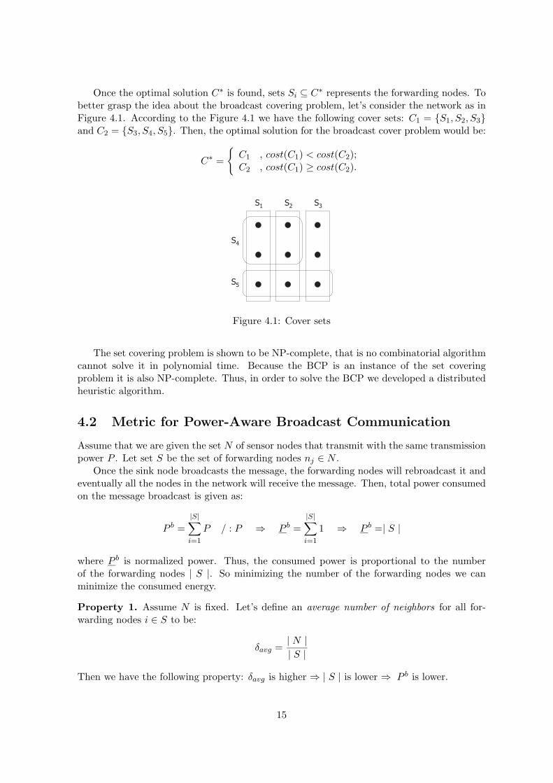
Once the optimal solution C∗ is found, sets Si ⊆ C∗ represents the forwarding nodes. Tobetter grasp the idea about the broadcast covering problem, let’s consider the network as inFigure 4.1. According to the Figure 4.1 we have the following cover sets: C1 = {S1, S2, S3}and C2 = {S3, S4, S5}. Then, the optimal solution for the broadcast cover problem would be:
C∗ ={
C1 , cost(C1) < cost(C2);C2 , cost(C1) ≥ cost(C2).
S1
S2
S3
S4
S5
Figure 4.1: Cover sets
The set covering problem is shown to be NP-complete, that is no combinatorial algorithmcannot solve it in polynomial time. Because the BCP is an instance of the set coveringproblem it is also NP-complete. Thus, in order to solve the BCP we developed a distributedheuristic algorithm.
4.2 Metric for Power-Aware Broadcast Communication
Assume that we are given the set N of sensor nodes that transmit with the same transmissionpower P . Let set S be the set of forwarding nodes nj ∈ N .
Once the sink node broadcasts the message, the forwarding nodes will rebroadcast it andeventually all the nodes in the network will receive the message. Then, total power consumedon the message broadcast is given as:
P b =|S|∑i=1
P / : P ⇒ P b =|S|∑i=1
1 ⇒ P b =| S |
where P b is normalized power. Thus, the consumed power is proportional to the numberof the forwarding nodes | S |. So minimizing the number of the forwarding nodes we canminimize the consumed energy.
Property 1. Assume N is fixed. Let’s define an average number of neighbors for all for-warding nodes i ∈ S to be:
δavg =| N || S |
Then we have the following property: δavg is higher ⇒ | S | is lower ⇒ P b is lower.
15

Property 1 implies that a good choice for the forwarding nodes would be nodes that caninclude in a covered set, by rebroadcasting, the higher number of new nodes (those whichhave not yet received a broadcast message). Besides, our objective is to maximize the lifetimeof each node in the network. Hence, we also include and remain battery capacity of a nodeinto account when deciding on whether the node should be the forwarding one.
With the above properties, we define the broadcast cost function as follows. We observenode j. Let’s C be a set of nodes which are already covered, that is, they have received abroadcast message. Consequently, Cc would be the set containing the nodes which have notyet received a broadcast message. Let Nj be a set of neighboring nodes of node j.
If node j would rebroadcasts, the number of nodes δ(j) that would be newly included inset C, is:
Sj = Nj ∩ Cc
δ(j) =| Sj |Finally, the broadcast cost function if defined to be:
cbj =
ejx1(Ej
Ej)x2
[δ(j)]x3(4.1)
where cbj is the broadcast cost of node j (cost(Sj)), ej is the consumed energy on rebroad-
casting a message, Ej is the initial energy at the receiving node j, Ej is the residual energyat the receiving node j, and x1, x2, x3 are nonnegative weighting factors.
The broadcast cost function 4.1 shows that the desirability of using the node j as theforwarding node increases if its energy spent per newly included node decreases.
4.3 Distributed Heuristic Solution for the BCP
As stated in Section 4.1, the BCP is a NP-complete problem and hence a heuristic is used tosolve it. Our heuristic uses the wireless multicast advantage property of the wireless channel.In order to elaborate our approach, let’s observe a set of nodes as shown in Figure 4.2.
i j
Oij
Ni
Rj
Nj
Uj = Nj - Oij
Figure 4.2: An overlapping set of two nodes
For nodes i and j we denote their neighbor sets as Ni and Nj , respectively. We defineoverlapping set Oij as a set that contains the nodes that fall into both node i’s and node j’sneighbor sets (transmission ranges). The main idea of the defined sets is that node j, once
16

it has received a broadcast message form node i, can learn which of the nodes from itsneighbor set Nj have also received the message sent by node i. Apparently, the nodes thatare contained in overlapping set Oij are those that have also received the message. We definethe neighbors of node j, which have received the message, as covered. The neighbors of nodej that have not yet received the message are said to be uncovered, and we denote this set asUj . Apparently, Uj = Nj −Oij .
The basic idea behind such an approach is that node j need not rebroadcast the messageif all of its neighbors have been covered by the previous transmissions, that is if Uj =ø.
We now describe our algorithm, shown in Figure 4.3. The algorithm is divided into twophases. In the first phases, each node in the network calculates overlapping sets for all itsneighbors. For this purpose each node transmits HELLO packets to its neighbors. Insidethe HELLO packets each node puts all its current neighbors. Upon receiving the HELLOpacket, a node calculates the overlapping sets by comparing the nodes contained in the packetwith its neighbors. This phase can called an initialization phase, the one in which the nodeslearn their neighborhoods.
In the second phase each node, upon receiving a broadcast message, uses its overlappingsets to make a decision whether to rebroadcast the message. Apparently, if a node finds themessage’s uncovered set empty, it will not rebroadcast that particular message. If, on theother hand, the node’s uncovered set is not empty the node will wait for some random timeperiod before it rebroadcasts the message. If during that period the node receives a duplicatemessage, but from a different neighbor, it will recalculate the uncovered set for the message.Then, if the uncovered set is not empty, the node will again wait for the random time periodbefore it rebroadcasts the message.
Figure 4.3: Distributed algorithm for the BCP
A crucial issue in our algorithm is an appropriate choice for the random time period anode has to wait before if retransmits. In order to manage this, we used the broadcast cost(defined in the previous section) that is assigned to each node in the network. Thus, as canbe seen in Figure 4.3, the upper bound for the random time period depends on the broadcastcost of a node. The ratio � cb
i
cb0� represents a normalized broadcast cost, while ∆ is a constant
17

time period. Now, the random time period is found by means of the function that returns arandom number distributed uniformly between 0 and � cb
i
cb0� ×∆. Consequently, the expected
duration of the waiting period, for the nodes with lower broadcast costs, will be shorter thenfor those nodes with higher broadcast costs. This mean that the nodes with the smallerbroadcast costs are given a probability advance to rebroadcast before the nodes with higherbroadcast costs.
One important problem we have to cope with is a problem of ensuring reliability. We wantto ensure that each node receives all broadcast messages sent by the source node. As our mainconcern is a power-aware broadcast protocol, we assume that the lower-layer communicationprotocols (MAC etc.) ensure reliability.
Our algorithm has an interesting property: it implicitly avoids collisions. This is due tothe fact that each node in the network waits for some random period before it transmits abroadcast message, which in turn results in a low probability of the collision occurrence (thisis similar to 802.11 MAC protocol).
Another important advantage of our approach to the broadcast problem is that it considerstransmission powers of the nodes. In order to explain this, let’s observe node i, and let’s defineits transmission power Pi as:
Pi ≡ {Pij | Pik ≤ Pij ,∀k ∈ Ui}
where Pij is the transmission power at which node i has to transmit in order to reach node j.The main idea behind the above definition is that the node i, when it receives a broadcast
message, adapts its transmission power according to the uncovered set. Thus, the requiredtransmission power of node i may be lower because its most distant neighbor may be alreadycovered.
4.4 Broadcast Simulations
Our goal was to evaluate the power-awareness and scalability characteristics of the proposeddistributed broadcast algorithm. We performed the simulations in GloMoSim [10]. GloMoSimis a scalable simulation environment for wireless and wired network systems.
The MAC layer protocol used in the simulations is IEEE standard 802.11 DistributedCoordination Function (DFC). In all simulations, radio range is the same for every sensornode, and is equal to 300 meters. The channel capacity is 19.2 kbits/sec. This is taken fromthe common specification for the sensor networks. The propagation model used is known asfree space [5].
During a simulation one node acts as the source of broadcast messages. As can be seenin Figure 4.3, each node maintains a queue of messages that the node receives during waitingto retransmit. In order to avoid the implementation of the queue, we simply delay thebroadcast messages and thus avoid the aggregation of the messages on a node. In this waywe also refrained a possible negative impact of the 802.11 MAC layer on the simulation results[11].
Because we used the same radio range for every node, the cost function 4.1 was slightlymodified. Thus we implemented the cost function of the following form:
cbj =
(Ej
Ej)1
[δ(j)]1
18

Node costs are updated constantly and when a broadcast message is transmitted. Wemodelled the battery consumption of the nodes in the following way. Initially, every nodehave the same battery capacity. When node i transmits a message its battery capacity BCi
is reduced by an amount that is proportional with the duration of the transmission ∆i, thatis, BCi = BCi − ∆i × PT , where PT is a constant that represents power consumption intransmit.
In order to learn their neighbors and to calculate their overlapping sets, in our implemen-tation, every node sends a HELLO message every 4 seconds.
The simulations were performed using networks of four different sizes: 50, 100, 200, and400 nodes, respectively. For each network we used 9 different deployment regions for thenodes in order to build networks with the different node densities. The nodes were deployedusing uniform random distribution. In each simulation 100 broadcast messages are sent bythe source node. The mean number of forwarding nodes is calculated for each simulation.
Figure 4.4 shows the achieved ratio of non-rebroadcasting nodes for each of different-sizedand different dense networks.
4 5 6 7 8 9 10 11 12 130
10
20
30
40
50
60
70
80
90
100
average node degree
ratio
of t
he n
on−
rebr
oadc
astin
g no
des
[%]
50 nodes 100 nodes 200 nodes 400 nodes analytical bound (50 nodes)
Figure 4.4: The ratio of non-rebroadcasting nodes
We can see that if each node in the network executes our simple broadcast mechanismthe ratio of the forwarding nodes will be sufficiently small. Thus, for example if the averagenode degree (average number of neighbors) is 8, our algorithm achieves that more then 60%of the nodes do not participate in the re-broadcasting of a particular broadcast message.Figure 4.4 reveal that our distributed algorithm also has good scalability properties. Thus,if the average node degree is 8, the difference of ratios of the non-rebroadcasting nodes, fordifferent network sizes, is between 4 and 10%.
As we expected, the ratio of the non-rebroadcasting nodes rises with the density of anetwork. Figure 4.4 also shows an analytically obtained bound for different network config-urations. In APPENDIX B we explained an approach to obtain the bound.
19

We also simulated the impact of the broadcast algorithm to the remaining battery capacityof nodes. For this purpose, we choose one node and vary its initial battery capacity. We areinterested in the number of messages for which this particular node acted as a forwardingnode. Figure 4.5. shows us that the ratio of messages, relayed by this particular node,decreases as the node’s battery capacity decreases, which is desirable behavior. However,it is important to notice that this property has a negative impact on the total number offorwarding nodes. Thus the trade-off between minimizing the number of forwarding nodesand evenly distributing energy load is necessary.
4 5 6 7 8 9 10 11 12 130
10
20
30
40
50
60
70
80
90
100
average node degree
ratio
of t
he r
elay
ed m
sgs
[%]
initially full battery initially 50% discharged battery initially 80% discharged ba ttery
Figure 4.5: The ratio of relayed messages
20

Conclusion
We have presented two distributed algorithms for power-aware dissemination of data in wire-less sensor networks. The proposed algorithms use metrics that take into account remainingbattery capacities of the sensor nodes and thus evenly distribute the energy load among thenodes. We have shown that a simple localized algorithm executed at each node suffices toachieve an energy efficient dissemination of data in this networks. In addition this guaranteesgood scalability characteristics of our dissemination mechanisms.
For unicast routing, we have shown how the minimum cost topology (multiple spanningtree rooted at one hop neighbors of the sink node) can be built on a wireless network. Forthis purpose, we have used the link base model. With our algorithm, a node will eventuallyhave multiple paths to the sink node. Consequently, the fault tolerance is increased. With amultiple path to the sink node, the nodes can employ different policies for the route selection.
In respect to the broadcast issue, we have defined the broadcast covering problem, whosemain concern is to minimize total broadcast costs of covering a sensor network. We haveshown how a simple concept of overlapping sets can be used to solve the broadcast prob-lem, or to make the total number of the forwarding nodes sufficiently small. Moreover, ourbroadcast algorithm evenly distributes the energy load among the nodes in the network. Oursimulation demonstrated that a simply randomized heuristic, used by our algorithms, resultsin satisfactory scalability and energy efficient characteristics.
21

APPENDIX A
In this appendix we propose two methods for building the link cost matrix. As shownin Section 3.1, a cost of link between two neighboring nodes is given by equation 3.1. Thusa node, in order to build its link cost matrix, needs the following information for each ofits neighbors: the consumed energy for unit information transmission between the node andnode’s neighbor, the neighbor initial and residual energy.
Method 1 As shown in Section 2.1, the wireless sensor’s propagation model is found to bethe long-distance path loss model, that is:
AdB(r) = AdB(1m) + 10n log r + adB (6.1)
Attenuation AdB(r) in equation 6.1 represents the power that a transmitter must radiatein order to reach distance r.
Let’s now consider node s and all the nodes that fall into the transmission range of nodes. Once node s boots up, it will broadcast HELLO messages to its neighbors. All thenodes within the transmission range of node s will eventually receive a HELLO message andmeasure the received signal level.
Let’s denote the received signal level at some node i with PRi, and the transmission powerof node s with PTs . Node i will reply to node s measured signal level PRi and its normalizedresidual energy Ei
Ei. Hence node s can compute a value of attenuation along the path to
receiving node i, that is,
AdB(ri) = PTs(d)[dBm]− PRi [dBm] (6.2)
With AdB(ri) and normalized residual energy EiEi
of node i, node s can compute the costcsi of the link between nodes s and i.
Method 2 In this method node s scans its neighborhood by sending HELLO messages atdifferent transmission power levels PTs . The transmission power level is changed in smallsteps. Within each HELLO message, node s sends information of transmission power levelat which the message was sent.
After receive a HELLO message, node i will reply to node s its normalized residual energyand transmission power level it finds in the HELLO message. Thus node s can learn the powerat which it must transmit in order to reach node i, and it can learn the residual energy ofnode i. Consequently, node s can compute the cost csi of the link between nodes s and i.
22

APPENDIX B
In this appendix we explain our approach to getting the analytical bound for the results ofthe simulations in Figure 4.4.
Let’s observe a network shown in Figure 6.1. We assume node i forwards a broadcastmessage that is received by node j. It is clear that the number of newly included nodes, byretransmission of node j, will be maximized if the distance between nodes i and j, which wedenote dij , is equal to the transmission range of these nodes. Assuming that each forwardingnode includes maximum number of new nodes in the cover set, a strong upper bound on thenumber of the forwarding nodes can be obtained as follows:
Nf =N
Nmax
where Nf is the number of the forwarding nodes, N is the total number of nodes in thenetwork, and Nmax is the number of nodes that a forwarding node can include in the coverset by single retransmission when the distance dij is equal to the transmission range of nodes.
It is easy to see that this strong bound on the number of the forwarding nodes is notachievable in the networks in our simulations. For this reason we take the average distancebetween nodes and its neighbors, which we denote davg, as a distance between two forwardingnodes that are in the transmission range of each other. Then, the bound to the number of theforwarding nodes, for a network of size N , is calculated according to the following expression:
Nf =N
Navg
where Navg is the number of nodes that would be newly included in the cover set by singleretransmission of a forwarding node when the distance dij = davg.
i j
dij
i j
dij
Figure 6.1: Size of the uncovered set for a different distance between the forwarding nodes
23

Bibliography
[1] G.J. Pottie and W.J. Kaiser. Wireless integrated network sensors. Communication ofthe ACM, 43(5):51–58, May 2000.
[2] G. Asada, M. Dong, T.S. Lin, F. Newberg, G. Pottie, and W.J. Kaiser. Wireless in-tegrated network sensors: Low power systems on a chip. Technical report, RockwellScience Center, 1999.
[3] Volkan Rodoplu and Teresa H. Meng. Minimum energy mobile wireless networks. IEEEjournal on selected areas in communications, 17(8), August 1999.
[4] J. E. Wieselthier, G. D. Nguyen, and A. Ephremides. On the construction of energy-efficient broadcast and multicast trees in wireless networks. In IEEE, 2000.
[5] Theodore S. Rappaport. Wireless communication: Principles and Practice. PrenticeHall, 1996.
[6] Elizabeth M. Royer and Chai-Keong Toh. A review of current routing protocols for adhoc mobile wireless networks. IEEE Personal Communications, 6(2):46–55, April 1999.
[7] Suresh Singh, Mike Woo, and C. S. Raghavendra. Power-aware routing in mobile adhoc networks. In The fourth annual ACM/IEEE international conference on Mobilecomputing and networking, pages 181–190. ACM, 1998.
[8] J.H. Chang and L. Tassiulas. Energy conserving routing in wireless ad-hoc networks. InProceedings of IEEE INFOCOM00. ACM, 2000.
[9] Levente Buttyan and Jean-Pierre Hubaux. Nuglets: a virtual currency to stimulatecooperation in self-organized mobile ad hoc networks. Technical report, Swiss FederalInstitute of Technology, Lausanne, January 2001.
[10] L. Bajaj, M. Takai, R. Ahuja, K. Tang, R. Bagrodia, and M. Gerla. Glomosim: Ascalable netwrork simulation environment. Technical report, University of California atLos Angeles, 1999.
[11] Shugong Xu and Tarek Saadawi. Does the ieee 802.11 mac protocol work well in multihopwireless ad hoc networks? IEEE Communications Magazine, 36(6), June 2001.
24