adaptive energy-aware transmission scheme for wireless sensor
TRANSCRIPT
Adaptive Energy-Aware Transmission Scheme forWireless Sensor Networks
Abdullahi Ibrahim Abdu
Submitted to theInstitute of Graduate Studies and Research
in partial fulfillment of the requirements for the Degree of
Master of Sciencein
Computer Engineering
Eastern Mediterranean UniversityMay 2011
Gazimağusa, North Cyprus

Approval of the Institute of Graduate Studies and Research
Prof. Dr. Elvan YılmazDirector
I certify that this thesis satisfies the requirements as a thesis for the degree of Masterof Science in Computer Engineering.
Assoc. Prof. Dr. Muhammed SalamahChair, Department of Computer Engineering
We certify that we have read this thesis and that in our opinion it is fully adequate inscope and quality as a thesis for the degree of Master of Science in ComputerEngineering.
Asst. Prof. Dr. Muhammed SalamahSupervisor
Examining Committee
1. Assoc. Prof. Dr. Hasan Demirel
2. Assoc. Prof. Dr. Isik Aybay
2. Assoc. Prof. Dr. Muhammed Salamah
3. Asst. Prof. Dr. Gurcu Oz
iii
ABSTRACT
A Wireless Sensor Network is composed of a large number of sensor nodes that are
densely deployed either inside a phenomenon or very close to it [1]. A WSN enables
wide range of applications; as a result it is receiving increasing research interest. The
main challenge to researchers in the field of WSNs is to maintain a useful network
lifetime under constrains imposed on the limited energy reserves that are inherent in
the small, locally-powered sensor nodes. This research addresses this challenge
through the development and evaluation of an information control, energy
management and, transmission range adaptation algorithm which leads to an
increased network lifetime.
The contribution of this research is the development of an AIRT (Adaptive
Information managed energy-aware algorithm for sensor networks with Rule
managed reporting and Transmission Range Adjustments) or AIRT. The AIRT
scheme increases the network lifetime at the possible sacrifices of often trivial data
and further increase network lifetime through adapting transmission ranges based on
nodes energy reserve level and message importance. The wireless sensor network
environment was simulated using C Programming Language, where several runs of
the simulation were performed in other to get reliable performance results. The
performance results showed the advantage of the proposed AIRT scheme. Two
different set of network statistics were measured; nodes energy resource depletion
time and network connectivity. The results of each statistics of our technique were
compared to the results of the statistics of similar works of recent researchers and our

iv
results show a significant improvement in network lifetime and connectivity (though
not the focus of this research)
Keywords: Energy-aware; wireless sensor networks; adaptive transmission
ranges; priority balancing.
v
ÖZ
Kablosuz sensör ağı çok sayıda bağlantı noktasının bir olgu içinde bir araya
gelmesinden oluşur. Bu ağların uygulama alanları çok geniştir ve halen büyüyen bir
araştırma alanıdır. Kablosuz sensör ağlarını araştıran araştırmacıların üzerinde
yoğunlaştıkları bir konu, kullanılabilir ağ yaşam süresini belli kısıtlamalarla
düzenleyip (limitli enerji kaynakları gibi) küçük bölgesel olarak güçlendiren sensör
bağlantı noktalarıyla çalışmasını sağlamaktır.
Bu araştırmanın katkısı uyan IRT algoritmasını geliştirmek ve AIRT algoritmasını
bulmaktır. AIRT, ağ yaşam süresini arttırır, paketin önemlilik derecesine ve bağlantı
noktasının enerji kaynağına göre transfer alanını ayarlar. Çalışmada, kablosuz sensör
ağının simulasyonu C programlama dili kullanılarak yapıldı. Program, daha gerçekçi
sonuçlar vermesi için birkaç kez çalıştırıldı. Üç değişik ağ istatistiği ölçüldü. Bunlar,
bağlantı noktasının enerji kaynaklarını tüketme zamanı, ağ bağlantısı ve paket
başarısıdır. Elde edilen sonuçlar diğer çalışmalarla karşılaştırıldı ve bu çalışmanın
sonuçlarının ağ yaşam süresi, bağlantı ve kaybolan paketlerde önemli bir gelişme
gözlendi.
Anahtar kelimeler: Enerji-koruması, kablosuz ağ bağlantısı, adaptif tarnsfer
alanları, öncelikli dengeleme.

vi
DEDICATION
To My Parents

vii
ACKNOWLEDGMENTS
This thesis would not have been possible without the infinite mercy of Almighty
Allah (Subhanahu Wa Ta'ala) He says; “Be! And it is” (Baqarah, 117).
I am heartily thankful to my supervisor, Dr. Muhammed Salamah, for his
encouragement, guidance, patience and support during my bachelor degree and
especially during my master’s degree thesis.
I would like to thank my brother and colleague Mr. Zhavat Sherinov for his advices
and ideas. I’m also thankful to my friend Miss Gozde Sarisin for doing my Ozet.
I owe my deepest gratitude to my Mum Mrs. Fatima Shehu who undoubtedly has
given me the support no human can ever give me. I remember you always tell me
that “I should hold on, it will be over soon” and indeed you are right. May Allah
reward you with Jannatul Firdaus, ameen. And also my Dad Mr. Ibrahim Abdu, who
has done all what a Dad needs to do for his child and more, you are the best Dad
anybody can ever have. I remember you always tell me “I’m the first born and I
should site a good example for my siblings”, I will inshaAllah always make you
proud. May Allah reward you with Jannatul Firdaus, ameen.
I would like to show my gratitude to my siblings; Yusuf Abdu (Babalayyo), Ibrahim
Abdu (Kapa Appa), and Aisha Abdu (Hajja Addare) for their concern and moral
support throughout my life and during my thesis. BarakAllahufeekum.

viii
TABLE OF CONTENTS
ABSTRACT................................................................................................................. iii
ÖZ................................................................................................................................. v
DEDICATION ............................................................................................................. vi
ACKNOWLEDGMENT.............................................................................................. vii
LIST OF TABLES........................................................................................................ xi
LIST OF FIGURES ..................................................................................................... xii
ABBREVIATIONS .................................................................................................... xiv
1 INTRODUCTION ...................................................................................................... 1
1.1 Research aims ...................................................................................................... 2
1.1.1 Major Research Contributions ....................................................................... 3
2 CRITICS OF WSN STATE-OF-THE-ART ................................................................ 5
2.1 Introduction to WSNs .......................................................................................... 5
2.2 Research Facts ..................................................................................................... 9
2.3 Energy Management .......................................................................................... 10
2.3.1 Energy Harvesting....................................................................................... 11
2.3.2 Energy-Aware Algorithms........................................................................... 13
2.3.3 Discussion................................................................................................... 15
2.4 Information Management ................................................................................... 15
2.4.1 Information Propagation.............................................................................. 15
2.4.1.1 Continuous/Periodic Propagation.......................................................... 16
2.4.1.2 Query Driven Propagation .................................................................... 16
2.4.1.3 Event Driven Propagation ..................................................................... 17
2.4.2 Discussion................................................................................................... 18
ix
2.5 Transmission Range Adjustments ...................................................................... 19
2.5.1 Discussion................................................................................................... 20
2.6 COMMUNICATION AND NETWORKING FOR WSNS ................................ 20
2.6.1 Communication Architecture of a WSN ...................................................... 21
2.6.2 Introduction to Networking Protocol and Stacks .......................................... 21
2.6.3 Medium Access Control Layer .................................................................... 25
2.6.4 Networking Layer ....................................................................................... 26
2.6.4.1 Geographic Routing Algorithms ............................................................ 28
2.6.4.2 Energy-Aware Routing Algorithms........................................................ 28
2.6.4.3 Flooding-Based Routing algorithms....................................................... 28
2.6.5 Discussion................................................................................................... 30
2.7 WSNs SIMULATOR AND ENERGY MODELS .............................................. 31
2.8 SUMMERY....................................................................................................... 32
3 AIRT ........................................................................................................................ 34
3.1 Overview of AIRT ............................................................................................. 35
3.2 RMR.................................................................................................................. 37
3.3 IDEALS............................................................................................................. 38
3.4 TRA................................................................................................................... 39
3.5 Discussion and Summery ................................................................................... 44
4 PERFORMANCE MEASUREMENT....................................................................... 45
4.1 Simulation Setup................................................................................................ 45
4.2 Simulation of AIRT Algorithm .......................................................................... 47
4.3 Simulation Results ............................................................................................. 50
4.4 Discussion ......................................................................................................... 56
5 CONCLUSIONS ...................................................................................................... 57
x
REFERENCES............................................................................................................ 60
APPENDIX ................................................................................................................. 67
Appendix A Performance Measurement Raw Data ...................................................... 68
A.1 Energy depletion times of the four Simulations ................................................. 68
A.2 Network connectivity for Traditional simulation ............................................... 70
A.3 Network connectivity for IDEALS/RMR simulation ......................................... 71
A.4 Network connectivity for IRT simulation .......................................................... 72
A.5 Network connectivity for AIRT simulation........................................................ 73
Appendix B Performance Measurement Source Codes................................................. 76

xi
LIST OF TABLES
Table 2.1: Devices with fixed amount of energy stores…………………………..12
Table 2.2: Devices with fixed amount of power generation……………………...13
Table 3.1: Intuitionally determined transmission ranges………………………….42
Table 4.1: Simulation parameters………...………………………………………..47
Table 4.2: Percentage improvement of AIRT scheme in terms of connectivity…..53
xii
LIST OF FIGURES
Figure 2.1: Architecture of a typical wireless sensor nod……………………………6
Figure 2.2: Sensor Network Structure….………………………………………….....7
Figure 2.3: Outline of sensor network applications………………………………......8
Figure 2.4: Randomly deployed sensor nodes……………………………………....21
Figure 2.5: Computer Network Layering Architectures…………………………….22
Figure 2.6: A Three-dimensional stack…...……………………...………………….25
Figure 2.7: Various routing communication topologies…………………………….27
Figure 2.8: Flooding-based algorithm example……………………………………..29
Figure 3.1: Overview of AIRT System Diagram……………………………………35
Figure 3.2: RMR Operation…………………………………...…………………….36
Figure 3.3: IDEALS Operation……………………………………………………...38
Figure 3.4: Priority Allocation and Balancing Process……………………………...39
Figure 3.5: Transmission Range Adjustment Operation…………………………….40
Figure 3.6: Proposed AIRT system diagram………………………………………...41
Figure 3.7: Proposed AIRT Flowchart………………………………………………43
Figure 4.1 A snap shot of randomly distributed nodes used in the simulation……...46
Figure 4.2 Flowchart of AIRT simulation…………………………………………..49
Figure 4.3 Node energy depletion times…………………………………….............51
Figure 4.4 Traditional………….……………………………………………………53
Figure 4.5 IDEALS|RMR…..……………………………………………………….54
Figure 4.6 IRT…..…………………………………………………….......................54

xiii
Figure 4.7 AIRT…..…………………………………………………………………55

xiv
ABBREVIATIONS
WSN: Wireless Sensor Network
AIRT: Adaptive Information managed energy-aware algorithm for sensor networks
with Rule managed reporting and Transmission range adjustments
RMR: Rule Managed Reporting
IDEALS: Information manageD Energy-Aware aLgorithm for Sensor networks
TRA: Transmission Range Adjustments
MP: Message Priority
PP: Power Priority
DB: Data Base
T: Threshold
P: Periodic
D: Differential
MAC: Medium Access Control
OSI-BRM: OSI Basic Reference Model
Sim: Simulator
1
Chapter 1
INTRODUCTION
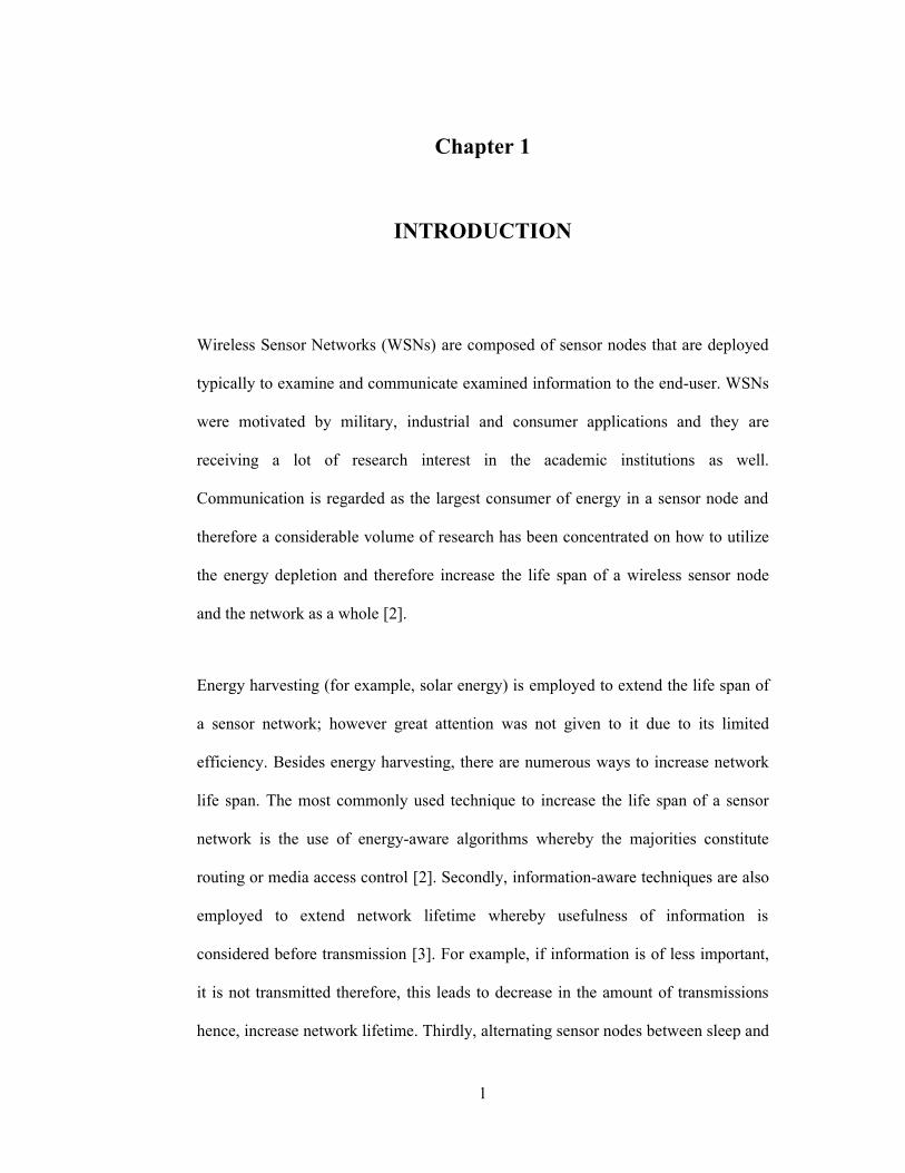
Wireless Sensor Networks (WSNs) are composed of sensor nodes that are deployed
typically to examine and communicate examined information to the end-user. WSNs
were motivated by military, industrial and consumer applications and they are
receiving a lot of research interest in the academic institutions as well.
Communication is regarded as the largest consumer of energy in a sensor node and
therefore a considerable volume of research has been concentrated on how to utilize
the energy depletion and therefore increase the life span of a wireless sensor node
and the network as a whole [2].
Energy harvesting (for example, solar energy) is employed to extend the life span of
a sensor network; however great attention was not given to it due to its limited
efficiency. Besides energy harvesting, there are numerous ways to increase network
life span. The most commonly used technique to increase the life span of a sensor
network is the use of energy-aware algorithms whereby the majorities constitute
routing or media access control [2]. Secondly, information-aware techniques are also
employed to extend network lifetime whereby usefulness of information is
considered before transmission [3]. For example, if information is of less important,
it is not transmitted therefore, this leads to decrease in the amount of transmissions
hence, increase network lifetime. Thirdly, alternating sensor nodes between sleep and
2
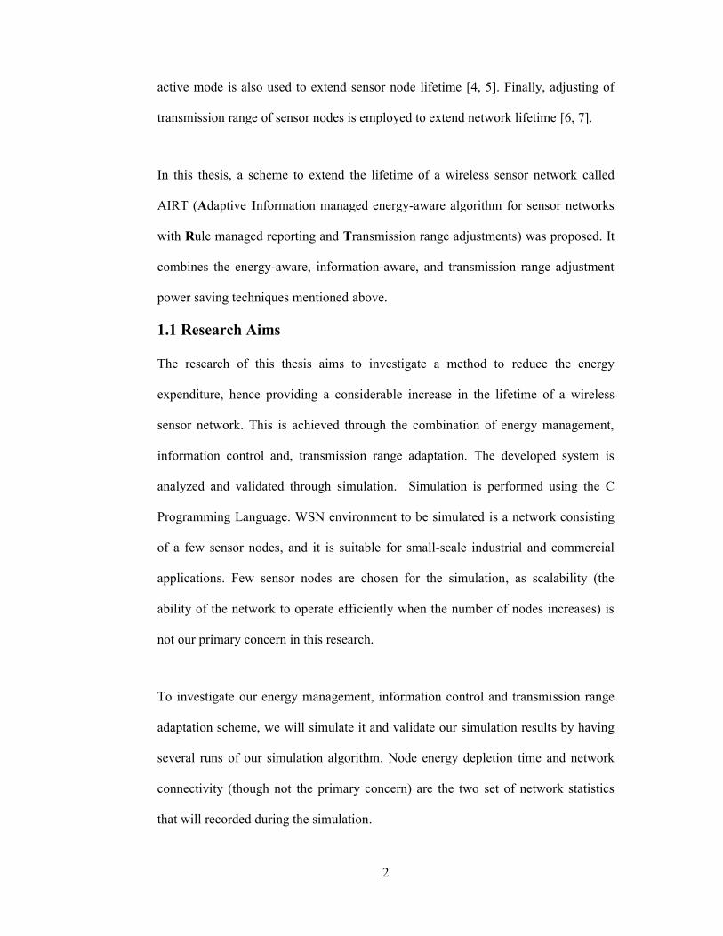
active mode is also used to extend sensor node lifetime [4, 5]. Finally, adjusting of
transmission range of sensor nodes is employed to extend network lifetime [6, 7].
In this thesis, a scheme to extend the lifetime of a wireless sensor network called
AIRT (Adaptive Information managed energy-aware algorithm for sensor networks
with Rule managed reporting and Transmission range adjustments) was proposed. It
combines the energy-aware, information-aware, and transmission range adjustment
power saving techniques mentioned above.
1.1 Research Aims
The research of this thesis aims to investigate a method to reduce the energy
expenditure, hence providing a considerable increase in the lifetime of a wireless
sensor network. This is achieved through the combination of energy management,
information control and, transmission range adaptation. The developed system is
analyzed and validated through simulation. Simulation is performed using the C
Programming Language. WSN environment to be simulated is a network consisting
of a few sensor nodes, and it is suitable for small-scale industrial and commercial
applications. Few sensor nodes are chosen for the simulation, as scalability (the
ability of the network to operate efficiently when the number of nodes increases) is
not our primary concern in this research.
To investigate our energy management, information control and transmission range
adaptation scheme, we will simulate it and validate our simulation results by having
several runs of our simulation algorithm. Node energy depletion time and network
connectivity (though not the primary concern) are the two set of network statistics
that will recorded during the simulation.
3
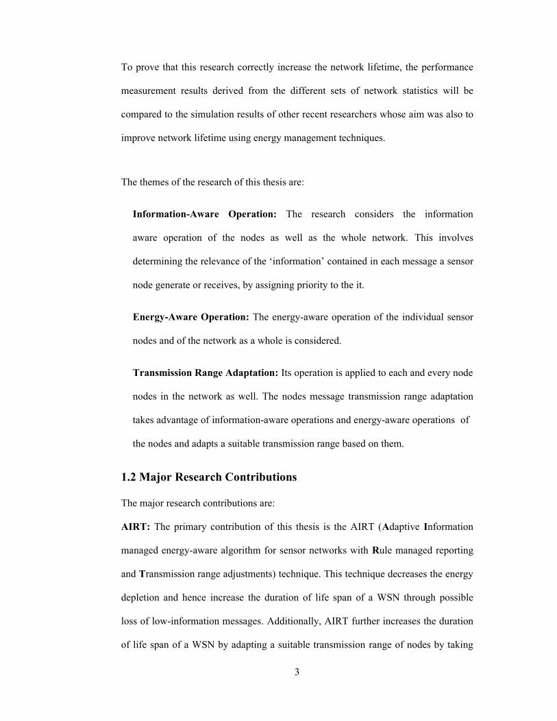
To prove that this research correctly increase the network lifetime, the performance
measurement results derived from the different sets of network statistics will be
compared to the simulation results of other recent researchers whose aim was also to
improve network lifetime using energy management techniques.
The themes of the research of this thesis are:
Information-Aware Operation: The research considers the information
aware operation of the nodes as well as the whole network. This involves
determining the relevance of the ‘information’ contained in each message a sensor
node generate or receives, by assigning priority to the it.
Energy-Aware Operation: The energy-aware operation of the individual sensor
nodes and of the network as a whole is considered.
Transmission Range Adaptation: Its operation is applied to each and every node
nodes in the network as well. The nodes message transmission range adaptation
takes advantage of information-aware operations and energy-aware operations of
the nodes and adapts a suitable transmission range based on them.
1.2 Major Research Contributions
The major research contributions are:
AIRT: The primary contribution of this thesis is the AIRT (Adaptive Information
managed energy-aware algorithm for sensor networks with Rule managed reporting
and Transmission range adjustments) technique. This technique decreases the energy
depletion and hence increase the duration of life span of a WSN through possible
loss of low-information messages. Additionally, AIRT further increases the duration
of life span of a WSN by adapting a suitable transmission range of nodes by taking

4
into consideration message importance and level of nodes energy resource. RMR
(Rule Managed Reporting) is an operation in AIRT that uses some defined system of
rules to check if the information contained in a message warrants it to be transmitted
and then give priority to the message. IDEALS (Information manageD Energy aware
ALgorithm for Sensor networks) is also an operation in AIRT that compared its
nodes residual energy level to the importance of message from RMR, then
determined if the message should be transmitted or not. Finally, TRA (Transmission
Range Adjustment) in AIRT determines a suitable transmission range for a node
based on the message priority from RMR and nodes residual energy level from
IDEALS and finally the message is transmitted with a suitable range.
The remaining part of the thesis research is organized as follows:
Chapter 2 presents some critiques of the state-of-the-art in the field of WSNs with
respect to energy management, information control, and transmission range
adaptation. Chapter 3 introduces the details of our AIRT algorithm developed in this
research. Chapter 4 provides the result obtained from the simulation of a WSN using
our developed AIRT algorithm. Chapter 5 concludes the report and outlines possible
future research.
5
Chapter2
CRITICS OF WIRELESS SENSOR NETWORKS STATE-
OF-THE-ART
In is important to note that WSNs are continuously receiving research interests in
academic as well as in many industrial and consumer applications till date. This
chapter provides an overview of some background information in the field of WSNs
with respect to energy management, information control, transmission range
adjustment, communication protocol, and simulation and energy modeling.
2.1 Introduction to Wireless Sensor Networks (WSNs)
Networks of wireless sensors are advantageous for both application and economical
reasons. They are beneficial for application reasons because they made possible the
applications that were previously not possible to achieve with wired sensors, some of
such application are monitoring environments under harsh weather conditions, and
monitoring hostile enemy territory. Additionally, the economic benefit of WSNs is
the lack of cabling between sensors. The cost of installing wiring for a single sensor
in a building is estimated to average $200 [8], or as much as $150 per meter for
critical applications in risky industrial environments [9]. It is suggested that a typical
industrial scenario can see a reduction of over 80% in the total system cost (for both
materials and installation labor) by using commercially available WSNs [10]. Hence,
introduction of wireless communication in sensor networks show a considerable cost
savings.
6
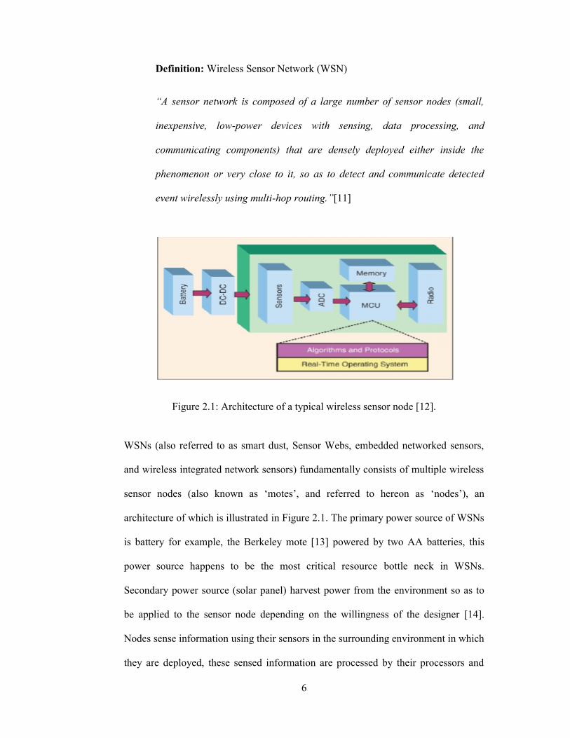
Definition: Wireless Sensor Network (WSN)
“A sensor network is composed of a large number of sensor nodes (small,
inexpensive, low-power devices with sensing, data processing, and
communicating components) that are densely deployed either inside the
phenomenon or very close to it, so as to detect and communicate detected
event wirelessly using multi-hop routing.”[11]
Figure 2.1: Architecture of a typical wireless sensor node [12].
WSNs (also referred to as smart dust, Sensor Webs, embedded networked sensors,
and wireless integrated network sensors) fundamentally consists of multiple wireless
sensor nodes (also known as ‘motes’, and referred to hereon as ‘nodes’), an
architecture of which is illustrated in Figure 2.1. The primary power source of WSNs
is battery for example, the Berkeley mote [13] powered by two AA batteries, this
power source happens to be the most critical resource bottle neck in WSNs.
Secondary power source (solar panel) harvest power from the environment so as to
be applied to the sensor node depending on the willingness of the designer [14].
Nodes sense information using their sensors in the surrounding environment in which
they are deployed, these sensed information are processed by their processors and
7
because sensor nodes have limited memory size and are naturally deployed in harsh
locations, a radio transceiver is implemented for wireless communication to transfer
the data to a base station (which could be a laptop) in accordance to a communication
protocol [15]. Wireless sensor nodes in the network forward and receive packets
among themselves so as to perform packet routing (deciding the path that a packet
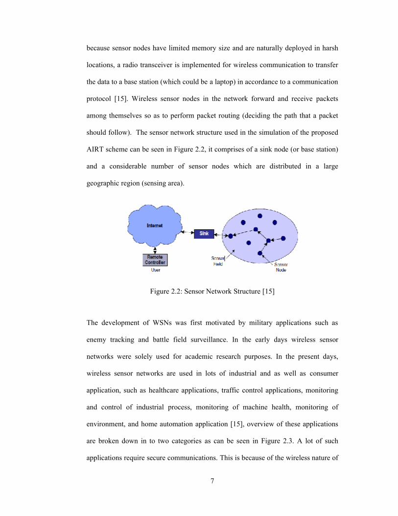
should follow). The sensor network structure used in the simulation of the proposed
AIRT scheme can be seen in Figure 2.2, it comprises of a sink node (or base station)
and a considerable number of sensor nodes which are distributed in a large
geographic region (sensing area).
Figure 2.2: Sensor Network Structure [15]
The development of WSNs was first motivated by military applications such as
enemy tracking and battle field surveillance. In the early days wireless sensor
networks were solely used for academic research purposes. In the present days,
wireless sensor networks are used in lots of industrial and as well as consumer
application, such as healthcare applications, traffic control applications, monitoring
and control of industrial process, monitoring of machine health, monitoring of
environment, and home automation application [15], overview of these applications
are broken down in to two categories as can be seen in Figure 2.3. A lot of such
applications require secure communications. This is because of the wireless nature of
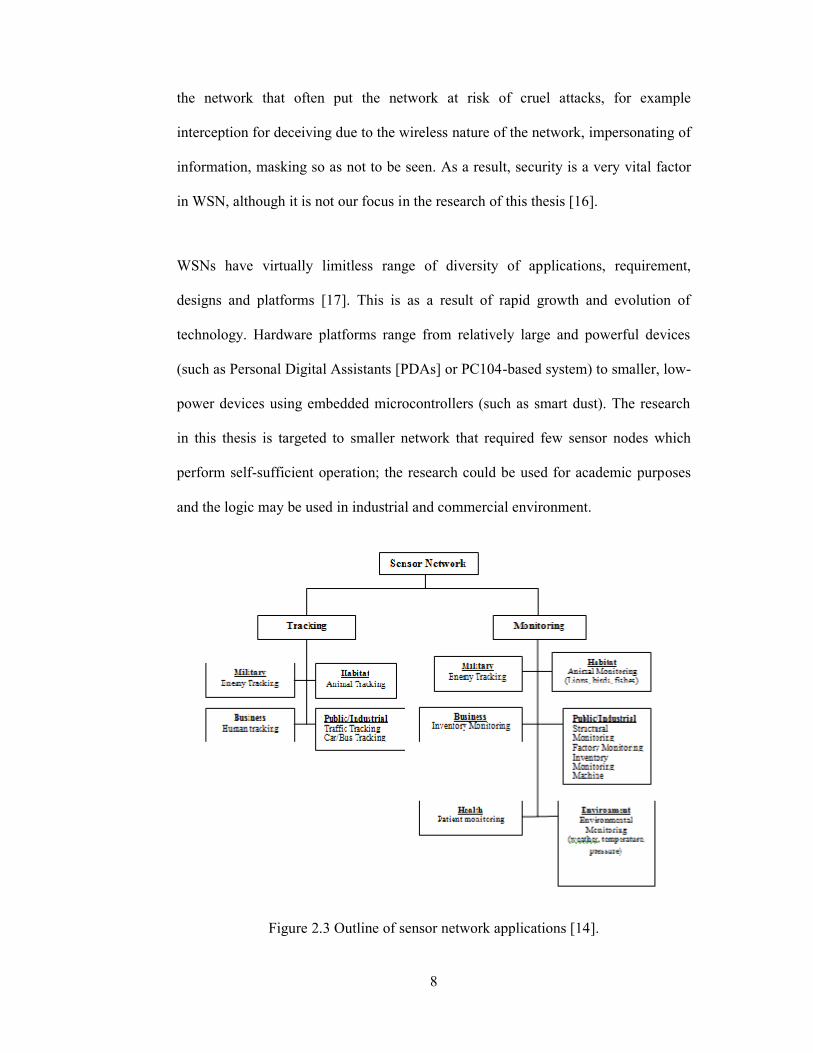
8
the network that often put the network at risk of cruel attacks, for example
interception for deceiving due to the wireless nature of the network, impersonating of
information, masking so as not to be seen. As a result, security is a very vital factor
in WSN, although it is not our focus in the research of this thesis [16].
WSNs have virtually limitless range of diversity of applications, requirement,
designs and platforms [17]. This is as a result of rapid growth and evolution of
technology. Hardware platforms range from relatively large and powerful devices
(such as Personal Digital Assistants [PDAs] or PC104-based system) to smaller, low-
power devices using embedded microcontrollers (such as smart dust). The research
in this thesis is targeted to smaller network that required few sensor nodes which
perform self-sufficient operation; the research could be used for academic purposes
and the logic may be used in industrial and commercial environment.
Figure 2.3 Outline of sensor network applications [14].

9
2.2 Research facts
Radio communication is regarded as the most power demanding operation in a
sensor node [11]. Wireless communication strength is reliant on how the sensor
nodes are organized. As we might guess, sparsely organized sensor nodes may lead
to long-range transmission and higher energy usage whereas densely organized
sensor nodes may lead to short-range transmission and less energy expenditure [14].
There are always tradeoffs in wireless sensor networks depending on the application.
However, power consumption still remains one the most important constraints in
WSNs. For that reason:
“Protocols must focus primarily on power conservation. They must have inbuilt
trade-off mechanisms that give the end user the option of prolonging network lifetime
at the cost of lower throughput or higher transmission delay.” [11]
Therefore in order to increase network lifetime of a wireless sensor network, energy
harvesting (e.g. solar energy) is an attractive option. Conversely, energy harvesting
management for WSNs has not received research interest comparable to that of other
related field; as it was disregarded as a research and development priority for the
Office of the Communications (OFCOM) in 2007 [18]. For this reason, it is not used
in this thesis as a mechanism to extend the network lifetime.
In this thesis, usefulness of data is a priority as oppose to treating all data as having
equal or homogeneous usefulness. “Transmitted information would have different
levels of usefulness/importance to the end user. For example, the information of a car
10
tire pressure sensor detecting a fast puncture requiring urgent action is more
important than knowing that everything okay” [19] .
2.3 Energy Management
Based on the numerous experimental studies in the field of wireless sensor networks
where low-power radio transceiver communication is in use, wireless radio
communication is often the most power-demanding operation in a sensor device [20].
This radio communication leads to rapid consumption of energy resource in each and
every sensor node and the network as a whole. For this reason, a considerable
volume of research has been reported investigating a wide range of methods for
reducing and controlling energy consumption [11, 20, 22]; some of which are
discussed in this section.
Techniques for dropping the energy depletion of a sensor node may include Dynamic
Voltage Scaling (DVS) and Dynamic Frequency Scaling (DFS). The former
decreases the voltage to conserve power, while the later decreases the frequency to
conserve power [21, 22]. As a result of this decrease, performance in traded;
however this trade is acceptable in many WSNs.
In a duty cycle operation, the majority of the cycle is spent in the low-power sleep
state following this cycle; sleep-wakeup-sample-compute-communicate [23]. For the
duration of the sleep period of a duty cycle operation in a WSN, vital events can be
missed, and also some applications and sensors require continuous sampling (for
example accelerometers) which restricts duty-cycle operation from being easily
achievable [24]. For these reasons, careful thought is given to duty-cycle-operation.

11
Authors in [25] proposed a technique to increase the time it takes for a sensor node to
completely deplete its network lifetime by scheduling between sleep and active mode
and adjusting node transmission range. And their simulation results show a
considerable increase in network lifetime compared to techniques that used either
duty-cycle or transmission range adjustments only.
Energy harvesting although it is not used in this thesis, we felt it is important to
mention that, as harvesting is continuously receiving research interest because it
helps to increase the energy source from zero energy to low energy. In the
subsections below, energy harvesting and energy-aware operations for WSNs will be
investigated.
2.3.1 Energy Harvesting
Energy harvesting can be defined as a process of obtaining energy from an external
source (e.g., solar power) to power small devices like sensor nodes. The motivating
factor behind using energy harvesting is to address the issue of limited energy store
inherent in small locally powered sensor nodes. Energy harvesting enables
applications that might not to possible achieve, for example in WSNs systems such
as Zigbee’s, when the battery of wireless node is deployed at a remote site is
unreliable or unavailable, energy harvesting can supply power. Additionally, locally
powered nodes that are sustainable through energy harvesting are useful in
applications where no wired infrastructure exists (for example, environmental
monitoring applications).
There are a wide variety of different energy sources appropriate for powering
wireless sensor nodes [8]. Table 2.1 and 2.2 shows a comparison of the typical
energy obtainable from a variety of different energy stores and sources considering

12
the energy that they could provide over a period of 10 years [8, 26]. Furthermore,
there is a large possibility for wearable applications of WSNs harvesting energy from
the human body from sources such as blood pressure, body heat, walking or
breathing [26].
To maximize the benefits obtained through energy harvesting, understanding and
management is required in a node’s embedded software; as will be discussed in the
next section.
Table 2.1: Devices with fixed amount of energy stores
Energy Source/Store Power / EnergyDensity
Energy Obtainedover Ten Years
Solar (Outdoors :Direct Sun) 15.0 mW/cm2 4.73 MJ/cm2
Solar (Outdoors: Cloudy) 0.15 mW/cm2 47.3 kJ/cm2
Solar (Indoors: Office Desk) 6.00 μW/cm2 1.89 kJ/cm2
Solar (Indoors: <60W Desk Lamp) 570 μW/cm2 180 kJ/cm2
Vibrations 10.0 - 250 μW/cm3 3.15 - 78.8 kJ/cm3
Acoustic Noise (75 - 100dB) 3.00 - 960 nW/cm3 0.0946 - 303 J/cm3
Air Flow (5% Efficient at 5m/s) 0.38 mW/cm3 120 kJ/cm3
Temperature (10C Differential) 15.0 μW/cm3 4.73 kJ/cm3
Human-Powered Systems (Shoe Inserts) 330 μW/cm3 104 kJ/cm3

13
Table 2.2: Devices with fixed amount of power generation (renewable energy
sources)
Energy Source/Store Energy Obtainedover Ten Years
Primary Batteries (Zinc-Air) 3.78 kJ/cm3
Primary Batteries (Lithium) 2.88 kJ/cm3
Primary Batteries (Alkaline) 1.20 kJ/cm3
Secondary Batteries (Li-ion) 1.08 kJ/cm3
Secondary Batteries (Ni-MH) 960 J/cm3
Secondary Batteries (Ni-Cad) 650 J/cm3
Micro-Fuel Cell 3.50 kJ/cm3
Heat Engine 3.35 kJ/cm3
Radioactive (63Ni) 1.64 kJ/cm3
2.3.2 Energy – Aware Algorithms
Energy aware algorithms for WSNs comprise of energy harvesting management,
topology control, duty cycle control and data processing, but the majority of the
algorithms constitute routing and media access control which will be discussed later
in this section.
In order to provide energy-aware operation, it is necessary to know that the general
definition of the lifetime of a WSN; it is the time between the deployed sensor nodes
start collecting data to the instance where the monitoring quality drops below an
acceptable threshold level [27]. The definition of the terms monitoring quality and
acceptable threshold level vary depending on the application the sensor nodes are

14
used for. For example, in an application that monitors the pressure of an agricultural
area, regular processing of 80% of the crops might be acceptable, however in a
military video surveillance application, a delay of 2s during surveillance might
trigger the threshold. As it was presented in Delin et al. [28] and Cianci et al. [29], if
a node’s energy store depletes past a preset threshold, the node enters a sleep state to
allow the energy store to be charged back to a sufficient level using energy
harvesting. The result of these controls the node’s sleeping behavior in the sense that,
nodes that have their residual energy levels below the threshold will sleep more
often. However, this will lead to data-forwarding-interruption problem.
Topology control algorithms (ASCENT [30] and Energy Conservation in WSN and
connectivity and graphs [31]) extend the lifetime of WSNs by taking advantage of
the redundancy of the network. If more than one node is sensing the same data, the
redundant nodes are selected and put in to sleep. When the energy of the sensing
nodes drops below an acceptable threshold, the sleeping nodes start sensing so that
the overall consumption is spread across the sensor node.
Occasionally in a WSN, in order to extend the network lifetime, we have to trade
computation processing accuracy. An example is a Finite Impulse Response (FIR)
filter or Fast Fourier Transform (FFT) [21], which is a common technique of
implementation that uses iterative algorithms which provide accurate results with
increased operational time. Consequently, by tolerating a less accurate result, the
operational time is reduced.
Up to this point, it is clear that radio transceiver in a sensor node, which is
responsible for radio communication is often the major consumer of energy in a

15
WSN, however, reducing the number of packets communicated results in a dramatic
energy reduction. Techniques and algorithms for Energy-aware information
extraction will be discussed in section 2.4.
2.3.3 Discussion
In Section 2.3, we tried to provide an overview of some relevant researches to the
energy management theme of this thesis. We discussed some techniques (such as,
energy harvesting management, topology control, and data processing) that are use to
extend the lifetime of a WSN and we discussed some energy sources (among which
are blood pressure, body heat, breathing, solar and vibration harvesting). This thesis
suggests that these low-power techniques and energy sources should be considered
carefully in all stages of design process of a sensor node.
2.4 Information Management
So far in our discussion, we made known that the major consumer of energy in a
sensor node is communication. We also observed that considering all data to be of
equal usefulness by communicating all data (redundant or trivial data) will be waste
of resource. That brings this thesis to the definition of information management,
which is a process of distinguishing useful data from redundant data so as to reduce
the rate of energy consumption in a sensor node and the sensor network at large. This
section will try to provide overview of research on information management for
WSNs, for the most part, information propagation will be explored.
2.4.1 Information propagation
Information propagation algorithm (or reporting technique) is defined as a process of
determining how data (which is sampled by a sensor node from its sensing
environment) should be made available to other nodes, sink node or the end-user.

16
Information propagation algorithms are in general more related to packet routing.
Below are the lists of four information propagation techniques [32, 33]:
1. Continuous/Periodic Propagation (data ‘pushing’)
2. Query-Driven Propagation (data ‘pulling’)
3. Even-Driven Propagation (data ‘pulling’)
4. Hybrid Propagation
2.4.1.1 Continuous/Periodic Propagation
In continuous propagation, deciding on the periodic duration has a significant effect
on the network performance. When a short periodic duration is chosen, packets will
be often propagated; this will lead a large portion of redundant or trivial data being
transmitted, hence consuming considerable amount of energy [34]. When a long
periodic duration is chosen, packets will be rarely propagated; the network suffers
from long delay and missing of events. While the missing of events may be avoided
by locally aggregating the average-max-min sensed values, this does not avoid the
issues of delay that aggregation introduces. Advantage of continuous propagation is
that it is suitable for applications with random or uncharacterized signal. Its
disadvantage is that does not minimize energy consumption or information
throughput. Query-driven and event driven propagation approaches provide more
suitable techniques, and will be discussed in the section below.
2.4.1.2 Query-Driven Propagation
In Query-driven approach to information propagation in WSNs, the user or
application initializes data transfer by querying data from the network [35]; for
example a query is propagated into the network requesting: “where in the building do
we have temperature about 35 degrees?” and appropriate nodes respond with packet
17
similar: “in x we have temperature above 35 degrees”. Additionally, query-driven
approach pulls data from a passive network to respond to query.
In [36], the authors Y. Yao and J. Gehrke, developed a Cougar approach which uses
a query-based propagation, the approach supports historic queries (for example,
“what is the average snow in 2003?”). Advantage of the approach is that it provides
the ability to store historic data; however it has a number of disadvantages. Firstly, in
order to respond to queries that require history, each node most have a database to
store the required information. Secondly, when any node is lost, it loses its entire set
of historical data.
Event-driven propagation is suitable for applications where users rarely or
infrequently draw information from the network (for example, users wish to know
about the temperature of a node only when they wish to know).
2.4.1.3 Event-Driven Propagation
In event-driven propagation, the sensor nodes are intelligent in the sense that they
decide for their selves when data should be reported to the sink node; for example a
packet is transmitted containing: “the temperature is too hot at location x”. Such
propagation systems can be classified into two categories:
a) The ones that report only the digital occurrence of an event (such as motion, and
smoke), and
b) The ones that report the occurrence and magnitude of an event (magnitude of
vibrations over a certain threshold) [24].
A. Manjeshwar and D.P. Agrawal in [37] proposed an event-base propagation
technique for WSN called TEEN. The technique is based upon the concept of two
18
thresholds: Ht (Hard Threshold) and St (Soft Threshold). When the sampled data
crosses the Ht or changes in the sensed data is more than St, data is then sent from the
sensor node. However, if neither of these two thresholds occurs, communication will
never take place meaning that data will never be sent to the user or sink node.
In Merrett et. al [38], the authors improved [37] even further by introducing IDEALS
(Information manageD Energy aware ALgorithm for Sensor networks). In IDEALS
technique, a node senses information and based on some user defined rules, priority
is given to this sensed information. Afterwards based on an energy-aware algorithm,
the packet is transmitted or not.
Aside from the information propagation techniques that use information to control
reporting discussed in the section above, there are other possible uses of information
control; such as: sample rate adjustment, packet reliability and bandwidth
management.
2.4.2 Discussion
Section 2.4 has outlined information management techniques in WSNs, focusing
more on information propagation. The disadvantage of periodic propagation was
discussed. Better propagation techniques (query-driven and event-driven) were also
investigated. Query–driven or data pulling (data pulled from the network in response
to queries sent by users or applications) technique. It has the advantage that it is
suitable for applications where users infrequently draw information from the
network. One of its disadvantages is that when a node containing history of event is
lost, all the history set of data in the node is also lost. In Event-driven or data pushing
(sensor node decides for itself when data should be reported to the sink, and pushes
data to the sink when required). Its advantage is that it does not transmit packet that

19
are trivial or redundant, hence decrease energy consumption. These event-based
detection algorithms are divided into two categories: rule-based approaches, and
predictive approaches. In the rule-based approach, the user defines what is important
to the application. In the predictive approach, nodes report quite a large amount of
data to enable the sampled environment to be reconstructed at the sink node.
Additionally, in rule-based approach, while requiring end-user input to define events
of importance, often provides the best method for event detection [39].
2.5 Transmission Range Adjustments
Based on our previous discussions, we have made known that the paramount concern
in WSNs is power scarcity, driven partially by energy resource (battery). In the
previous sections, we have investigated the researches done on energy management
and information control theme of this thesis. In this section, our aim is to give an
overview of a few researches done using transmission range adjustment to minimize
the energy consumption and hence, extend the network lifetime. Power saving
techniques can generally be classified into the following four categories: 1) Schedule
the wireless sensor node to swap between active and sleep mode. 2) Control power
by adjusting transmission range of wireless sensor node. 3) Energy efficient routing
and data gathering. 4) To reduce the amount of data transmitted and avoid useless
activity. In this section, we consider only power control by adjusting transmission
range of sensor node.
Cardei et al. in [40] presents an efficient method to lower the energy consumption by
organizing the sensors into a maximal number of disjoint sets that are activated
successively. Each disjoint set can monitor the entire target area and at the same time
propagate information to the sink node or end-user. Only one set at a time is put into

20
active mode (to monitor and propagate data), while other sets are put into low power
sleep mode.
Authors in [41] extend the work of [40] by considering a large number of sensors
with adjustable sensing range that are randomly deployed to monitor a number of
targets areas. Since the number of sensors is large and therefore they can redundantly
cover target areas, in order to conserve energy, sensors were organized in sets and
activated successively. A sensor can adjust its communication range by partaking in
multiple set covers, such that its total energy spent is constraint by the initial energy
resource of the sensor node.
2.5.1 Discussion
This section has outlined some works that applied transmission range adjustment and
significant amount of energy was incurred. It has also mentioned the four categories
of power saving techniques. Transmission range can be adjusted based on many
factors such as energy resource, message importance and redundancy of node
coverage. In this thesis, transmission range adjustment was based on a function or
two parameters (energy resource and message importance), details will come later in
subsequent sections.
2.6 Communication and Networking for WSNs
Wireless communication and networking in is a huge requirement in research,
design, implementation and operation of WSNs and computer network as a whole.
We will provide an overview of communication architecture and wireless networking
protocols applied to WSNs. In addition, MAC protocols in WSN and routing
algorithms will be discussed.
21
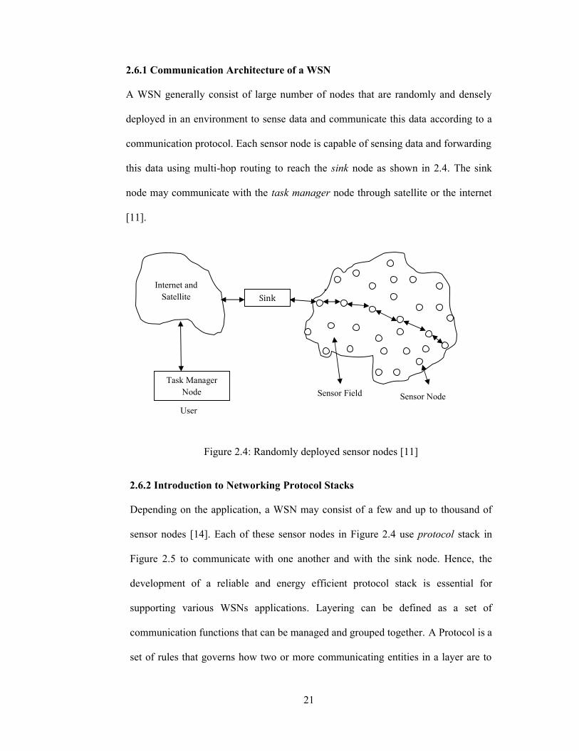
2.6.1 Communication Architecture of a WSN
A WSN generally consist of large number of nodes that are randomly and densely
deployed in an environment to sense data and communicate this data according to a
communication protocol. Each sensor node is capable of sensing data and forwarding
this data using multi-hop routing to reach the sink node as shown in 2.4. The sink
node may communicate with the task manager node through satellite or the internet
[11].
Figure 2.4: Randomly deployed sensor nodes [11]
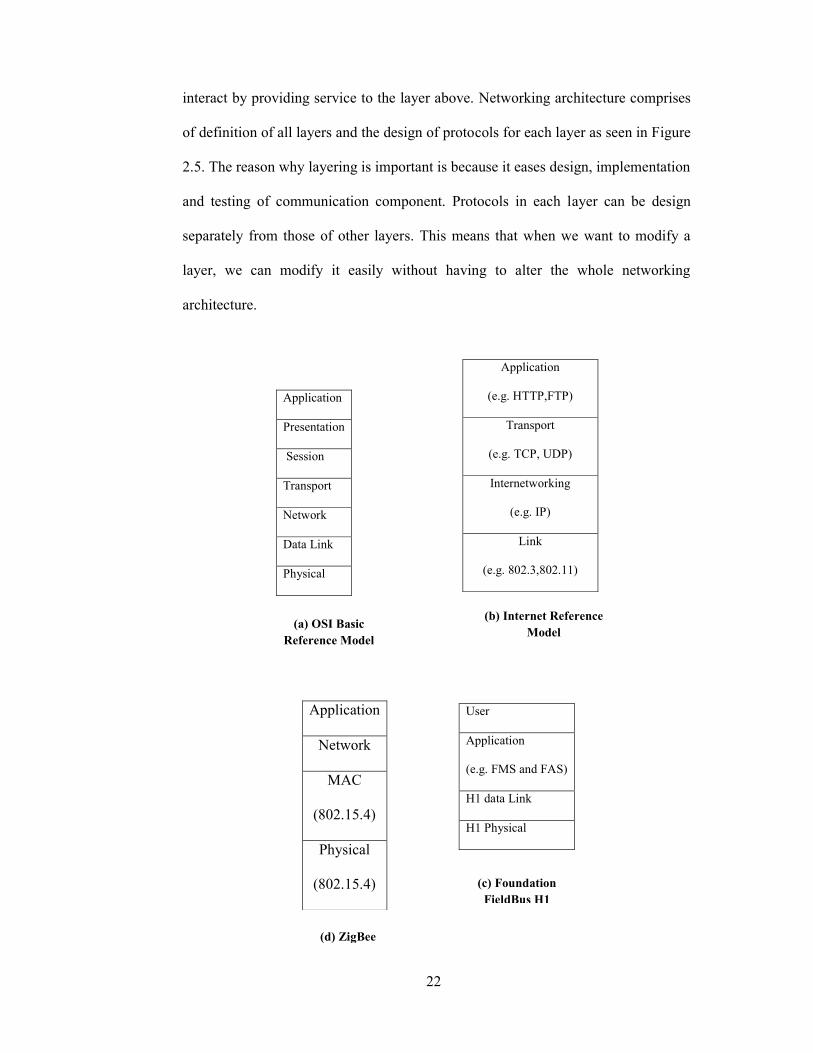
2.6.2 Introduction to Networking Protocol Stacks
Depending on the application, a WSN may consist of a few and up to thousand of
sensor nodes [14]. Each of these sensor nodes in Figure 2.4 use protocol stack in
Figure 2.5 to communicate with one another and with the sink node. Hence, the
development of a reliable and energy efficient protocol stack is essential for
supporting various WSNs applications. Layering can be defined as a set of
communication functions that can be managed and grouped together. A Protocol is a
set of rules that governs how two or more communicating entities in a layer are to
Sink
Task ManagerNode
Internet andSatellite
User
Sensor Field Sensor Node
22
interact by providing service to the layer above. Networking architecture comprises
of definition of all layers and the design of protocols for each layer as seen in Figure
2.5. The reason why layering is important is because it eases design, implementation
and testing of communication component. Protocols in each layer can be design
separately from those of other layers. This means that when we want to modify a
layer, we can modify it easily without having to alter the whole networking
architecture.
Application
Presentation
Session
Transport
Network
Data Link
Physical
Application
(e.g. HTTP,FTP)
Transport
(e.g. TCP, UDP)
Internetworking
(e.g. IP)
Link
(e.g. 802.3,802.11)
Application
Network
MAC
(802.15.4)
Physical
(802.15.4)
User
Application
(e.g. FMS and FAS)
H1 data Link
H1 Physical
(a) OSI BasicReference Model
(c) FoundationFieldBus H1
(b) Internet ReferenceModel
(d) ZigBee
23
Figure 2.5: (a) OSI Basic Reference Model (OSI-BRM) [42], (b) Internet Reference
Model [43], (c) Foundation Fieldbus H1 Stack [44], and (d) ZigBee Stack [45].
By the mid-1970s every computer vendor had developed its own proprietary layered
architecture. Problem arose when computers of different vendors try to network
together for communication. For that reason, OSI (Open standard interconnection –
Basic Reference Model) [42] which was an effort of ISO (International Organization
for Standards) enabled multivendor communication by proposing a basic layered
structure for communication shown in Figure 2.5. Many of the modern
communication protocols and models (such as the Internet Reference Model [45]
shown in Fig. 2.5) have modified OSI-BSM to suit their model requirements.
Furthermore, most if not all protocols for WSNs are also modified OSI-BSM. We
will evaluate the various energy-efficient protocols proposed for the transport layer,
network layer, and data-link layer, and their crosslayer interactions.
Transport Layer: The main goal of a transport layer protocol in a WSN is to
guarantee the reliability and quality of data in the sensor nodes (source and sink
nodes). Transport layer protocols in WSNs ought to support multiple applications,
variable reliability, packet-loss recovery, and congestion control mechanism [14].
Energy-efficient protocols proposed for transport layer are: Sensor Transmission
Control Protocol (STCP), Delay Sensitive Transport (DST), Event-to-Sink Reliable
Transport (ESRT), Price-Oriented Reliable Transport Protocol (PORT), Pump
slowly, fetch quickly (PSFQ) and GARUDA. Some of the characteristics of these
protocols are: DST, STCP, ESRT and PORT tackle the problem of congestion
control and reliability guarantee from the sensors to the sink whereas PSFQ and
GARUDA examine only the problem of reliability from the sink to the sensors.
24
Even though quite a large number of transport layer protocols have been proposed
for WSNs, there is still numerous open research problems, one of them is cross-layer
optimization. Crosslayer can be employed to improve the performance of transport
layer protocol by for example, selecting better path for retransmission.
Network Layer: The main aim of this layer is to manage the operation of the
network and route packet across the network from the source node to the sink node.
Details will be explored in later sections.
DataLink Layer: Datalink layer is concern by means of data transfer among two
nodes that share the same link. Given that the underlying network is wireless, there is
need for medium access control (MAC) and management for effective data transfer
[14]. More details on MAC protocol will we presented in the coming sections.
As was explained earlier that modern communication network architectures have
modified layers from the OSI-BRM to tailor the model to their specific requirements.
For example, Fieldbus H1 (which is one of the Foundation Fieldbus protocol
versions) [44] was designed as a network architecture for process control
applications, such as sensor networks. As can be seen from Figure 2.5, most of the
higher layers of the OSI-BRM are omitted because their functionality is not required
in Foundation Fieldbus H1. Additionally, Fieldbus H1 adds a user layer to the top
most part of the stack. The ZigBee specification [45] defines a low-cost, low-power
wireless communication standard that is mainly appropriate for WSNs. As can be
seen from Figure 2.5, many of the upper part of the OSI-BRM is discarded and even
the transport layer too, this is also because it is not needed in the ZigBee protocol
stack. MAC and Physical layer uses the IEEE 802.15.4.
A number of variations on the basic communication stack have been proposed in the
literature. One of them is the ‘three-dimensional’ stack for use with sensor networks

25
proposed by Akyildiz et at. [4]. As illustrated in Figure 2.6, besides having five
tradition layer from the OSI-BRM, three ‘management planes’ are added. These
management planes are added in order that sensor nodes can work together in a more
efficient way in term of power.
Figure 2.6: a ‘Three-dimensional’ stack [11].
2.6.3 Medium Access Control (MAC) Layer
MAC is traditionally a sub-layer of the data link layer, in traditional wireless
networks, it manages the usage of radio interface to ensure efficient utilization of
shared bandwidth and it balances throughput, delay and fairness. However in WSNs,
MAC protocol manages radio activity to conserve energy and it balance energy
efficiency as well. In WSNs, the primary performance metrics is usually energy
efficiency, while metrics such as scalability, adaptability to changes, latency,
throughput, fairness, and bandwidth utilization are of secondary importance. To
design an Energy-efficient MAC protocol, the following reasons for energy wastage
must be addressed [46].
Collision: When collisions occur at a node, the collided packets will be discarded
and retransmitted. Retransmission incurs huge energy consumption.

26
Idle Listening: Radio transceivers typically have four duty cycle states: transmitting,
receiving, listening (waiting to receive possible packet) and sleeping. Idle listening
waste significant amount of energy as it consumes the same energy as receiving.
Overhearing: Usually in sensor networks, packets are propagated over the network
using multi-hop routing (dissemination of packets from source to destination node,
whereby packets pass through intermediate nodes). Overhearing is when
intermediate nodes receive packet that they always have to retransmit.
Over Emitting: This involves transmitting packets to a destination that is not ready
to receive packets (either destination node is sleeping or some other reason), thus
causing retransmission which incurs huge energy wastage.
Below is a list of some MAC protocols used in the datalink layer of a WSNs. Details
can be found in [20, 46]:
- The B-MAC (Berkeley Berkeley Media Access Control) protocol
- The S-MAC (Sensor Media Access Control) protocol
- Wise MAC protocol
- The D-MAC (Data-gathering Media Access Control) protocol
- The Z-MAC protocol
2.6.4 Network Layer
The main function of network layer is to route packets from source to destination.
Routing protocols in WSNs differs from that of traditional routing protocols in
numerous ways [14]. Such that in traditional routing, internet Protocol (IP) based
routing is used to forward packets across the network, whereas in a WSN, sensor
nodes do not use IP addresses and therefore IP based routing protocols are not used
in them. Attention is given to lifetime of WSN for that reason; protocols ought to
meet network resource constraints for example limited energy, communication
27
bandwidth, memory, and computation capabilities so as to extend the network
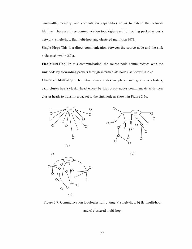
lifetime. There are three communication topologies used for routing packet across a
network: single-hop, flat multi-hop, and clustered multi-hop [47].
Single-Hop: This is a direct communication between the source node and the sink
node as shown in 2.7 a.
Flat Multi-Hop: In this communication, the source node communicates with the
sink node by forwarding packets through intermediate nodes, as shown in 2.7b.
Clustered Multi-hop: The entire sensor nodes are placed into groups or clusters,
each cluster has a cluster head where by the source nodes communicate with their
cluster heads to transmit a packet to the sink node as shown in Figure 2.7c.
(a)
(b)
(c)
Figure 2.7: Communication topologies for routing: a) single-hop, b) flat multi-hop,
and c) clustered multi-hop.
Sink
Sink
Sink
28
Many routing algorithms are constantly being proposed in the literature in other to
extend the network lifetime. In the section below, some of the proposed routing
algorithm in the literature such as flooding-based and energy-aware routing
algorithms will be investigated, moreover emphasis will be put on flooding-based
routing algorithm because it is assumed that the AIRT scheme in this thesis uses it to
route packets to the sink.
2.6.4.1 Geographic Routing Algorithms
Geographic (or location-aware) routing algorithms are algorithms that are suitable
for multi-hop routing in a dense network. Each node is assumed to know its location
and the location of its neighbors. The algorithm forwards packets by choosing
neighbors which are closest to the destination [14].
2.6.4.2 Energy-Aware Routing Algorithms
Authors in [38] introduced an energy-aware algorithm called IDEAL/RMR which
improves the lifetime of information with high priority. This increase in network
lifetime is achieved by considering the information contents of a packet and nodes
level of energy resource. IDEALS/RMR was further improved by our IRT scheme in
[48], whereby a sensor node adjusts its transmission range based on its level of
energy reserve. We improved our IRT scheme even better by introducing a new
scheme called AIRT, which improves the network lifetime of a sensor network by
adjusting nodes transmission range based on both level of energy reserve and
usefulness of information contents of the node.
2.6.4.3 Flooding-Based Routing algorithms
In this algorithm, nodes broadcast their packets to all of their neighboring nodes
except if they already forwarded the same kind of packet or if a maximum number of
hops have be reached or if the node is the packet’s destination.
29
Advantages: Among the many advantages are: simplicity in implementation,
scalability in the sense if more packets are added to the network the algorithm will
still remain efficient and robustness.
Disadvantages: Some of them are: implosion (copies of the same packets sent to the
neighboring nodes will be forwarded back to the sending node), and overlapping and
resource blindness.
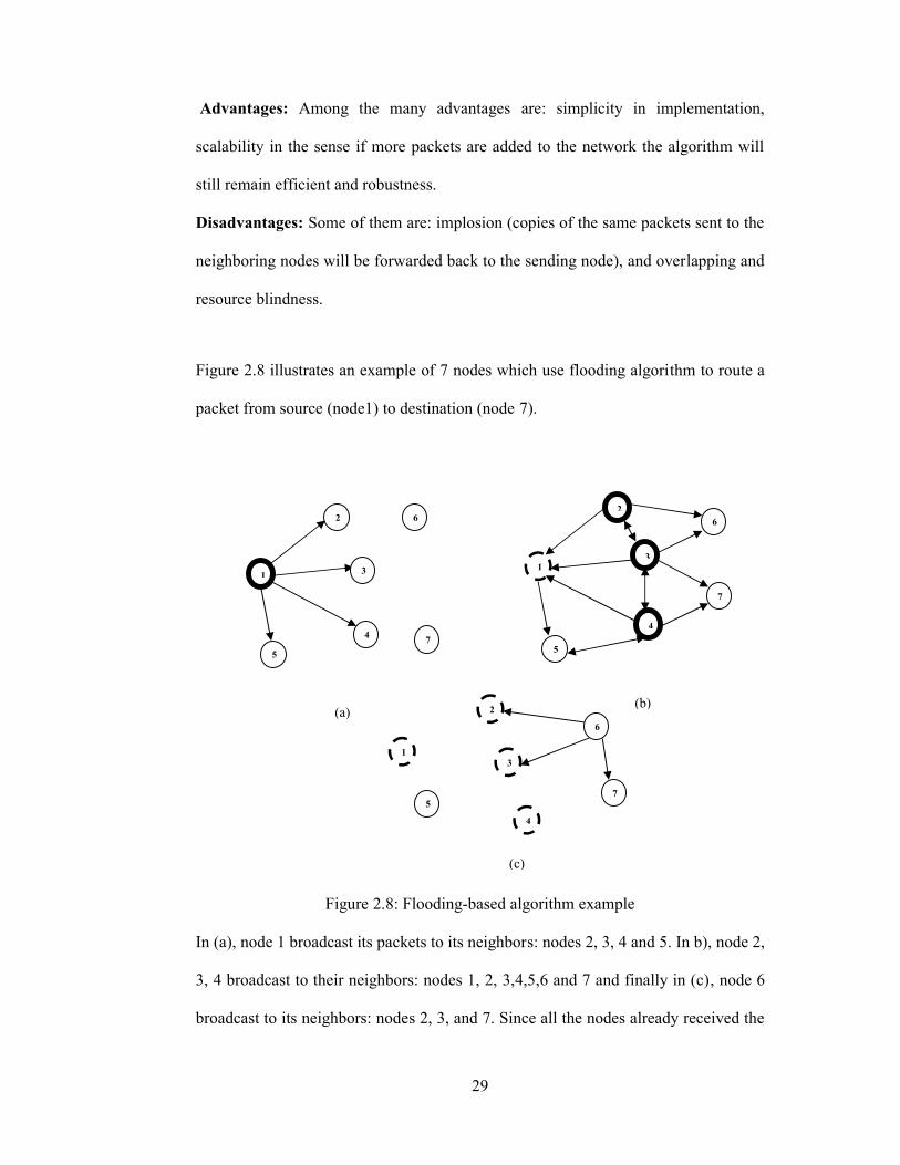
Figure 2.8 illustrates an example of 7 nodes which use flooding algorithm to route a
packet from source (node1) to destination (node 7).
Figure 2.8: Flooding-based algorithm example
In (a), node 1 broadcast its packets to its neighbors: nodes 2, 3, 4 and 5. In b), node 2,
3, 4 broadcast to their neighbors: nodes 1, 2, 3,4,5,6 and 7 and finally in (c), node 6
broadcast to its neighbors: nodes 2, 3, and 7. Since all the nodes already received the
2
3
45
1
6
7
1
2
3
4
5
6
7
1
5
2
3
6
4
7
(a)(b)
(c)

30
same packet and they don’t need it, they discard the packet except the destination
node 7 which process its received packet.
2.6.5 Discussion
In this section, we provided an overview of communication architecture and protocol
stacks in WSN. We proceeded further by briefly discussing MAC protocols and
routing algorithms though focusing on more relevant ideas to this thesis. We used a
clearly illustrated Figure to describe the communication architecture of a typical in
subsection 2.6.1. Designers of new and evolving applications and technologies use
the OSI model as their base for designing suitable communication architectures for
their applications. It was described that protocols in a layer can only communicate
with protocols in the layer directly above them however, with cross layering which is
a current research interest, protocols in a layer can communicate with non adjacent
layers, this is providing benefits to WSNs.
A MAC protocol which is part of datalink layer is for direct communication between
sensor nodes. Some factors are considered in the design of an energy efficient MAC
protocol such as idle listening, overhearing, collision and over emitting.
Finally, network protocols are mainly for end-to-end communication between source
and sink nodes. Many routing algorithms are proposed all the time in other to
minimize the energy consumption in WSNs. Among them is the energy-aware
algorithms have been considered, where a node decides on which route it should
follow based on its energy resource level. Lastly, flooding algorithm which due to its
simplicity it is usually adopted in WSNs, although it is highly inefficient in networks
that support only unicast communication.

31
2.7 WSN Simulators and Energy Model
A WSN can be analyzed by either practical implementation, analytical or simulation
programming. The most widely used method for analysis is simulation; this is mainly
because it is simple in modeling real WSN operations and easy to modify algorithms
and protocols. It can however be unrealistic because of assumptions that are made
during simulation; thus the realism of simulation depends on model it is based upon.
There are numerous WSN simulators developed, some of them are developed
particularly for a sensor network (such WSNsim [38]), while others are developed as
a simulation tool for WSN simulations (such as ns-2 [50]). In this thesis research we
analyzed a WSN and developed our AIRT algorithm by simulation using C
Programming Language.
Energy models means to model the energy resource (such as battery and energy
harvesting), and energy consumers (such as radio communication). There are many
energy models developed in the literature. In this thesis, the energy model proposed
by authors in [51] is considered; whereby the length of the packet in bits is
considered as a direction function of energy incurred through transmitting a packet.
The model provides equation for the energy needed by a sensor node to transmit
(2.2) and receive (2.3) a single packet in bits, where Eelec in Joules is the energy need
for the circuitry to transmit or receive a single bit, Eamp in Joules is the energy needed
for the transmit amplifier to transmit a single bit a distance of one meter.
Etx(l,d) = Eelecl + Eampld2 . (2.1)d = (x − x ) + (y − y ) . (2.2)
32
2.8 Summery
This section had investigated some of the background information in WSNs. Energy-
aware, information-aware, and transmission range adaptation themes of this thesis
were also explored. The chapter was then concluded by briefly discussing
networking protocols, simulators and energy models.
Many of the research in WSN is about how to lower the energy consumption, so as to
improve the network lifetime, this is mainly because WSNs are used in many
attractive applications and their batteries are difficult to replace. Therefore energy-
aware algorithms developed should carefully consider the nodes life time in all
operations.
Communication of sensed data across the network and to the sink node or end-user is
of paramount importance; therefore limiting the number of communicating
information can considerably increase the network lifetime. Most of researchers
consider information to be of equal importance in a WSN, thus they transmit this
information irrespective of whether it is important or not. However in this thesis, by
prioritizing nodes information a considerable increase in the network lifetime was
achieved. A number of information-aware algorithms were discussed and rule-base
which is the most efficient is used in this thesis.
Adjusting transmission range so as not to transmit information with the same single
transmission range is considered. Based on researches, it is observed that a great deal
of increase in network lifetime is achieved. It will be a good idea to consider it in
minimizing network consumption.

33
Network and datalink layer were also considered, where the focus was MAC
protocols for WSNs. The two categories of network simulators for evaluating WSNs
where discussed and examples of them were given. The energy model used in this
thesis was also mentioned in this chapter.
34
Chapter 3
AIRT: ADAPTIVE INFORMATION MANAGED
ENERGY-AWARE ALGORITHM FOR SENSOR
NETWORKS WITH RULE MANAGED REPORTING
AND TRANSMISSION RANGE ADJUSTMENTS
In chapter 2, some background information on wireless sensor networks focusing on
energy awareness was explored and most importantly, significance of power saving
techniques such as energy-aware, information-aware, and transmission range
adjustment were presented. This chapter presents AIRT (Adaptive Information
managed energy-aware algorithm for sensor networks with Rule managed reporting
and Transmission range adjustments) which extends the network lifetime based on
combination of energy-aware, information-aware, and transmission range operations.
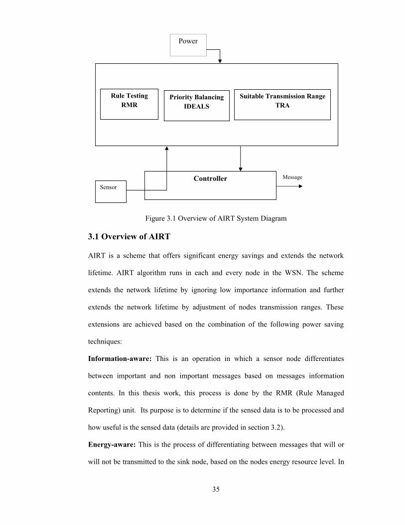
Section 3.1 presents an overview of the whole AIRT scheme; sections 3.2, 3.3, 3.4
present RMR, IDEALS, TRA operation units respectively. Figure 3.1 shows an
overview of the entire AIRT system. The overview of the system is shown so as to
give the reader an insight of the overall system which will be shown in details later in
the coming sections.
35
Figure 3.1 Overview of AIRT System Diagram
3.1 Overview of AIRT
AIRT is a scheme that offers significant energy savings and extends the network
lifetime. AIRT algorithm runs in each and every node in the WSN. The scheme
extends the network lifetime by ignoring low importance information and further
extends the network lifetime by adjustment of nodes transmission ranges. These
extensions are achieved based on the combination of the following power saving
techniques:
Information-aware: This is an operation in which a sensor node differentiates
between important and non important messages based on messages information
contents. In this thesis work, this process is done by the RMR (Rule Managed
Reporting) unit. Its purpose is to determine if the sensed data is to be processed and
how useful is the sensed data (details are provided in section 3.2).
Energy-aware: This is the process of differentiating between messages that will or
will not be transmitted to the sink node, based on the nodes energy resource level. In
Power
Rule TestingRMR
Priority BalancingIDEALS
Suitable Transmission RangeTRA
ControllerSensor
Message
36
this work, the operation is performed by the IDEALS (Information manageD Energy
Aware Algorithm for Sensor networks) unit (details are provided in section 3.3).
Transmission range adjustment: This is the process of adjusting of node’s
transmission range based on its energy resource level and importance of sensed data.
The TRA (Transmission Range Adjustment) unit is responsible for the operation
(details are provided in section 3.4).
The result of the union of information-aware, energy-aware and transmission range
adjustment mainly depends on the importance of sensed data and level of node’s
energy resource which we believe have never been considered by other researchers.
The key concept of the AIRT scheme is that a node which has high battery life
benefits the whole network by generating and forwarding messages and the node
does that with different node transmission ranges (based on importance of message
and energy resource level). However, a node with low battery life forwards only
messages which have high information contents and it does that with different
transmission ranges (based on message importance and energy resource level). By
performing these operations, AIRT extend the lifetime of important messages via
transmission range adjustment and the possible loss of messages of less important.
Figure 3.2 RMR Operation
37
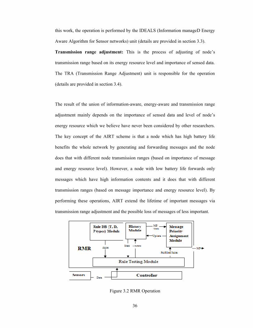
3.2 RMR
The operation of RMR unit depends on the set of rules defined by the designer to
decide on which data could be sensed and the level of importance of this sensed data
(some examples of user possible user defined rules are mentioned below). The
system diagram of RMR is given in Figure 3.2. Firstly, when the sensor node senses
data, the node passes the data to the controller, the controller then sends a value (e.g.
temperature) to the RMR (Rule Management Reporting) unit. The data is then
received by the Rule Testing Module, whose responsibility is to determine if the
event should be reported or not. It does that by checking the sensed data against the
rules in the Rule Database Module (getting history information about the previously
sensed values), simultaneously updates the history by adding the current information
of data and the sensed data to it. Rules may be triggered or not. Those rules which
are triggered are forwarded to the Message Priority Assignment module to determine
how important the content of the message is. It does that by assigning message
priorities (MP) to the triggered rules. This research uses five different MPs which are
(MP1-MP5). MP1 relates to the most important message which might represent
drastic change in the sensed data value. Conversely, MP4 - MP5 relates to the least
important packets which might represents slight or no change in the sensed value.
MP2 - MP3 relates to intermediate priorities packets which might represent moderate
change in the sensed value. The designer can enter any number of user defined rules;
these rules express different kind of events that the user is willing to detect in the
sensed region.
Examples of possible rules:
38
- Threshold rule [31]: This rule is applied when the current and last sensed
values (data such as pressure) are in opposite sides of the threshold value. For
example, “if the pressure rises above or falls below 70 Pascal”.
- Differential Rule [31]: This rule is applied when the dissimilarity among the
current and last sampled values is greater than some certain amount. For
example, “If the pressure of the current and last sensed value changes more
than 7 Pascal”.
- Periodic Rule [31]: This rule is applied when a specific defined rule has been
idle for a certain time duration, may be, “every 240 seconds”.
Figure 3.3 IDEALS Operation
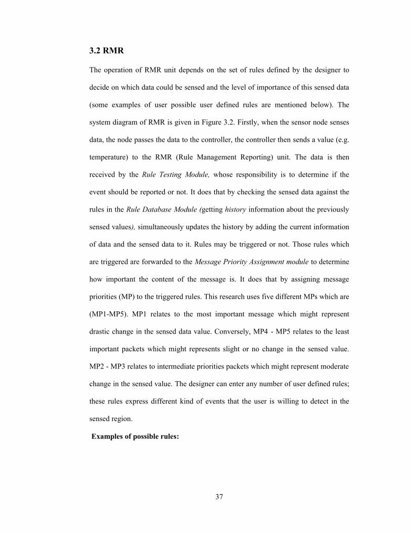
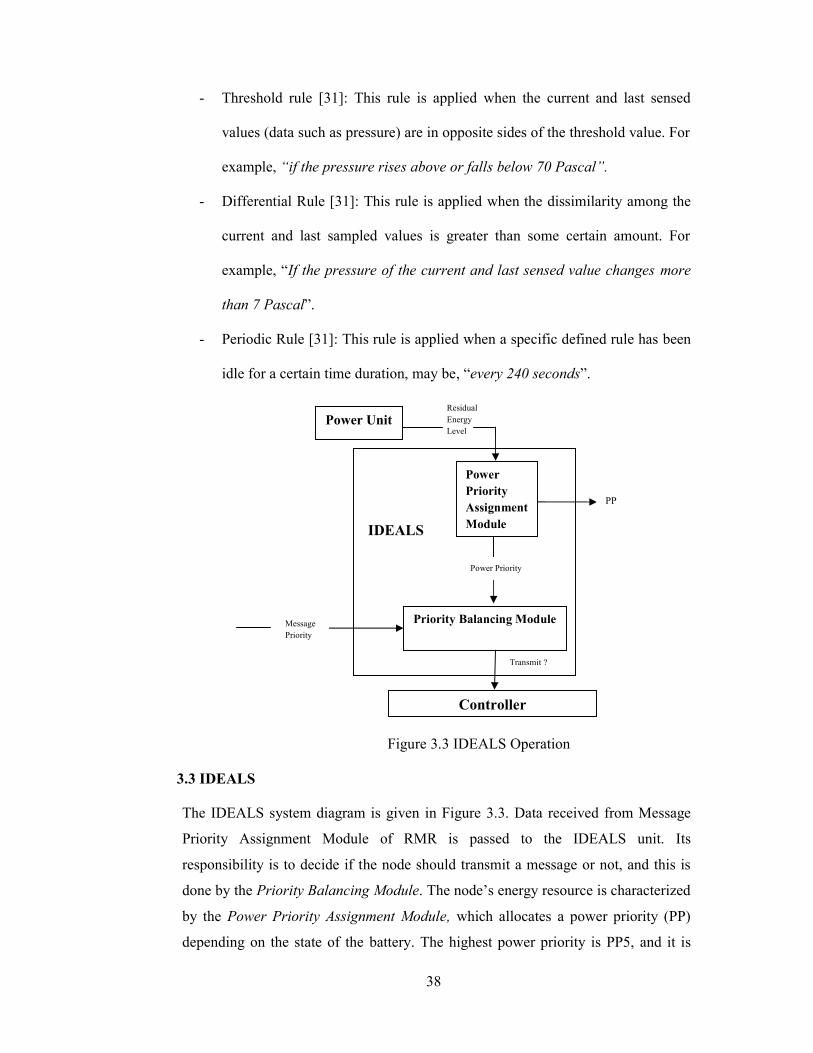
3.3 IDEALS
The IDEALS system diagram is given in Figure 3.3. Data received from Message
Priority Assignment Module of RMR is passed to the IDEALS unit. Its
responsibility is to decide if the node should transmit a message or not, and this is
done by the Priority Balancing Module. The node’s energy resource is characterized
by the Power Priority Assignment Module, which allocates a power priority (PP)
depending on the state of the battery. The highest power priority is PP5, and it is
Power UnitResidualEnergyLevel
PowerPriorityAssignmentModule
Power Priority
Priority Balancing Module
Transmit ?
MessagePriority
Controller
IDEALS
PP
39
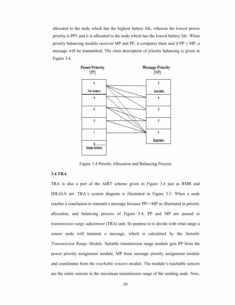
allocated to the node which has the highest battery life, whereas the lowest power
priority is PP1 and it is allocated to the node which has the lowest battery life. When
priority balancing module receives MP and PP, it compares them and if PP ≥ MP, a
message will be transmitted. The clear description of priority balancing is given in
Figure 3.4.
Figure 3.4 Priority Allocation and Balancing Process
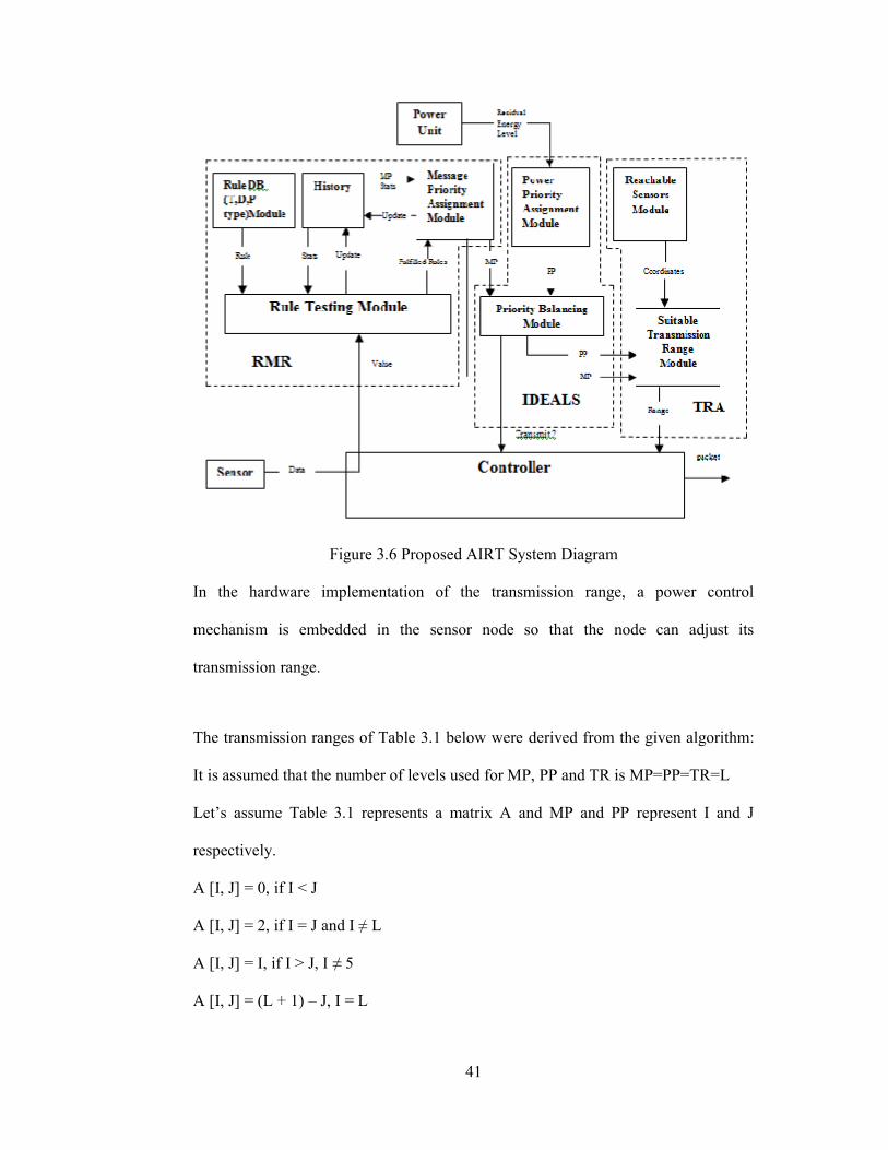
3.4 TRA
TRA is also a part of the AIRT scheme given in Figure 3.6 just as RMR and
IDEALS are. TRA’s system diagram is illustrated in Figure 3.5. When a node
reaches a conclusion to transmit a message because PP>=MP as illustrated in priority
allocation, and balancing process of Figure 3.4, PP and MP are passed to
transmission range adjustment (TRA) unit. Its purpose is to decide with what range a
sensor node will transmit a message, which is calculated by the Suitable
Transmission Range Module. Suitable transmission range module gets PP from the
power priority assignment module, MP from message priority assignment module
and coordinates from the reachable sensors module. The module’s reachable sensors
are the entire sensors in the maximum transmission range of the sending node. Now,
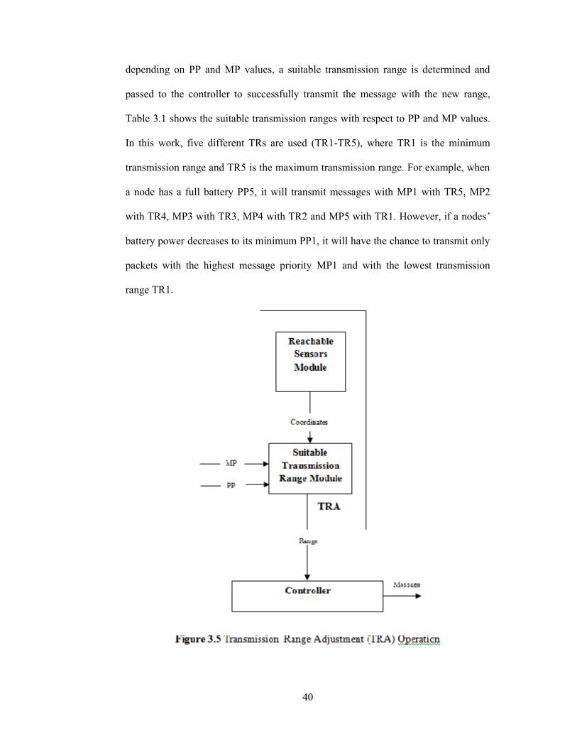
40
depending on PP and MP values, a suitable transmission range is determined and
passed to the controller to successfully transmit the message with the new range,
Table 3.1 shows the suitable transmission ranges with respect to PP and MP values.
In this work, five different TRs are used (TR1-TR5), where TR1 is the minimum
transmission range and TR5 is the maximum transmission range. For example, when
a node has a full battery PP5, it will transmit messages with MP1 with TR5, MP2
with TR4, MP3 with TR3, MP4 with TR2 and MP5 with TR1. However, if a nodes’
battery power decreases to its minimum PP1, it will have the chance to transmit only
packets with the highest message priority MP1 and with the lowest transmission
range TR1.
41
Figure 3.6 Proposed AIRT System Diagram
In the hardware implementation of the transmission range, a power control
mechanism is embedded in the sensor node so that the node can adjust its
transmission range.
The transmission ranges of Table 3.1 below were derived from the given algorithm:
It is assumed that the number of levels used for MP, PP and TR is MP=PP=TR=L
Let’s assume Table 3.1 represents a matrix A and MP and PP represent I and J
respectively.
A [I, J] = 0, if I < J
A [I, J] = 2, if I = J and I ≠ L
A [I, J] = I, if I > J, I ≠ 5
A [I, J] = (L + 1) – J, I = L

42
Table 3.1 Intuitionally determined transmission ranges
5 (Highest) 4 3 2 1 (Lowest)
5 (Lowest) 1(Min. TR) 0 0 0 0
4 2 2 0 0 0
3 3 4 2 0 0
2 4 4 3 2 0
1 (Highest) 5(Max. TR) 4 3 2 2
It should be noted that in AIRT scheme, a message may be dropped because of any
of the following scenarios: no message generation (that is a change in the sensed data
does not activate a rule), local priority unbalancing (meaning that if PP<MP, a
message will not be transmitted after it has been generated by a node), and routing
failure (that is to say there is no route for the packet to be propagated through the
network where PP≥MP due to loops, the packet will not be able to reach its
destination and therefore will be dropped).
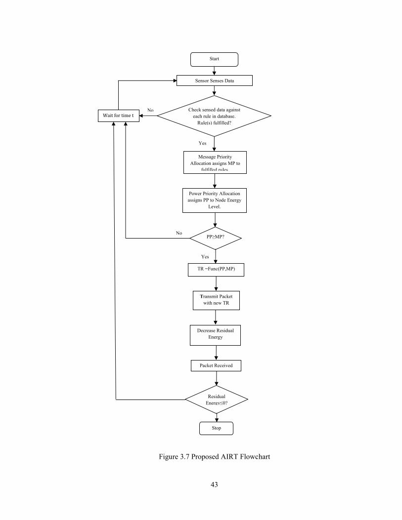
So far in this section, we discussed the overall AIRT system diagram operation and
the operations of information-aware, energy-aware and transmission range-aware
sub-systems. Figure 3.7 below illustrates the flow chart of the AIRT algorithm
developed in the thesis research.
MPPP
43
Sensor Senses Data
Check sensed data againsteach rule in database.
Rule(s) fulfilled?
PP≥MP?
ResidualEnergy≤0?
Stop
Figure 3.7 Proposed AIRT Flowchart
Start
Wait for time t
Message PriorityAllocation assigns MP to
fulfilled rules.
Power Priority Allocationassigns PP to Node Energy
Level.
TR =Func(PP,MP)
Transmit Packetwith new TR
Decrease ResidualEnergy
Packet Received
No
Yes
No
Yes
44
3.5 Discussion and Summery
This chapter has managed to describe the energy-aware, information-aware and
transmission range-aware theme of this thesis research via the introduction of AIRT
technique. AIRT technique is broken in to three parts (RMR, IDEALS, and TRA)
that perform separate operations, each of them could be modified or used as a whole
for further research on this topic. AIRT is a technique that extends the lifetime of a
WSN by ignoring low important packets and adjusting of nodes communication
range, which it is believed that based on this thesis research has never been
considered before. This is achieved through the union on information control (by
RMR), energy management (by IDEALS) and transmission range control (by TRA).
Considering the fact that no realistic scenario can be 100% efficient, the AIRT
scheme proposed in the thesis has quite a number of packet loss (sensed data not
matching any of the defined rules may be dropped, battery life less than packet
priority and during the propagation of packet in the network). Since a WSN is
application dependant, the AIRT technique proposed in this thesis research is
suitable for applications wherein events must be of different importance (it is not
suitable for applications that all events are of equal importance). So it is suggested
that AIRT or the operations (RMR, IDEALS and TRA) inside it should be modified
to suit a given application.
AIRT has the advantage of low complexity and low cost because complex
mathematical operations are not performed; it performs only comparisons and
increment operations which are known to be of low cost. Chapter 4 presents the
evaluation of AIRT through simulation.
45
Chapter 4
PERFORMANCE STUDY
Chapter 3 presented a discussion of the AIRT scheme, which is an energy-aware,
information-aware and transmission range algorithm for WSNs. This chapter
presents the evaluation of the AIRT scheme by simulation using the C Programming
Language to show its advantages. The AIRT technique is evaluated based on two
performance measures (network lifetime and connectivity) and it is compared with
other related energy saving techniques. The simulation results show a considerable
advantage of AIRT over other related energy saving schemes.
4.1 Simulation Setup
The simulation was performed using 20 sensor nodes in a network size of 70*70
meters. Each of the sensor nodes has the same maximum communication range of 20
meters. A predefined node placement topology has been considered in this
implementation. A snap shot of the network under simulation is shown in Figure 4.1.
The round dark dots correspond to sensor nodes and the links amongst them
correspond to the distance of communication (less than equal to 20meters) [31]. At
the beginning of the simulation, all sensor nodes have identical initial energy of 100
Joules [31], the equation for energy required to transmit a packet is shown in (1). The
simulation parameters are given in Table 4.1.
Etx(l,d) = Eelecl + Eampld2 [31]. (1)
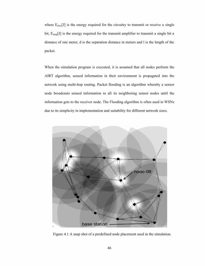
46
where Eelec[J] is the energy required for the circuitry to transmit or receive a single
bit, Eamp[J] is the energy required for the transmit amplifier to transmit a single bit a
distance of one meter, d is the separation distance in meters and l is the length of the
packet.
When the simulation program is executed, it is assumed that all nodes perform the
AIRT algorithm, sensed information in their environment is propagated into the
network using multi-hop routing. Packet flooding is an algorithm whereby a sensor
node broadcasts sensed information to all its neighboring sensor nodes until the
information gets to the receiver node. The Flooding algorithm is often used in WSNs
due to its simplicity in implementation and suitability for different network sizes.
Figure 4.1 A snap shot of a predefined node placement used in the simulation.
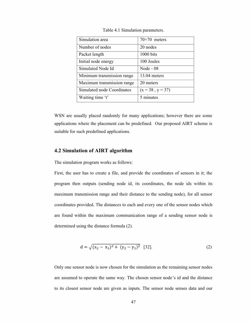
47
Table 4.1 Simulation parameters.
Simulation area 70×70 metersNumber of nodes 20 nodesPacket length 1000 bitsInitial node energy 100 JoulesSimulated Node Id Node - 08Minimum transmission range 13.04 metersMaximum transmission range 20 metersSimulated node Coordinates (x = 38 , y = 37)Waiting time ‘t’ 5 minutes
WSN are usually placed randomly for many applications; however there are some
applications where the placement can be predefined. Our proposed AIRT scheme is
suitable for such predefined applications.
4.2 Simulation of AIRT algorithm
The simulation program works as follows:
First, the user has to create a file, and provide the coordinates of sensors in it; the
program then outputs (sending node id, its coordinates, the node ids within its
maximum transmission range and their distance to the sending node), for all sensor
coordinates provided. The distances to each and every one of the sensor nodes which
are found within the maximum communication range of a sending sensor node is
determined using the distance formula (2).
d = (x − x ) + (y − y ) [32]. (2)
Only one sensor node is now chosen for the simulation as the remaining sensor nodes
are assumed to operate the same way. The chosen sensor node’s id and the distance
to its closest sensor node are given as inputs. The sensor node senses data and our
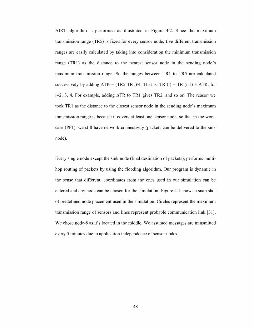
48
AIRT algorithm is performed as illustrated in Figure 4.2. Since the maximum
transmission range (TR5) is fixed for every sensor node, five different transmission
ranges are easily calculated by taking into consideration the minimum transmission
range (TR1) as the distance to the nearest sensor node in the sending node’s
maximum transmission range. So the ranges between TR1 to TR5 are calculated
successively by adding ΔTR = (TR5-TR1)/4. That is, TR (i) = TR (i-1) + ΔTR, for
i=2, 3, 4. For example, adding ΔTR to TR1 gives TR2, and so on. The reason we
took TR1 as the distance to the closest sensor node in the sending node’s maximum
transmission range is because it covers at least one sensor node, so that in the worst
case (PP1), we still have network connectivity (packets can be delivered to the sink
node).
Every single node except the sink node (final destination of packets), performs multi-
hop routing of packets by using the flooding algorithm. Our program is dynamic in
the sense that different, coordinates from the ones used in our simulation can be
entered and any node can be chosen for the simulation. Figure 4.1 shows a snap shot
of predefined node placement used in the simulation. Circles represent the maximum
transmission range of sensors and lines represent probable communication link [31].
We chose node-8 as it’s located in the middle. We assumed messages are transmitted
every 5 minutes due to application independence of sensor nodes.
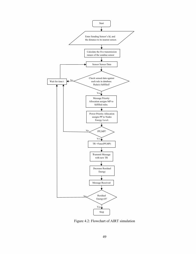
49
Enter Sending Sensor’s Id, andthe distance to its nearest sensor.
Calculate the five transmissionranges of the sending sensor
Sensor Senses Data
Check sensed data againsteach rule in database.
Rule(s) fulfilled?
PP≥MP?
ResidualEnergy≤0?
Stop
Figure 4.2: Flowchart of AIRT simulation
Start
Wait for time tmin.
Message PriorityAllocation assigns MP to
fulfilled rules.
Power Priority Allocationassigns PP to Nodes
Energy Level.
TR =Func(PP,MP)
Transmit Messagewith new TR
Decrease ResidualEnergy
Message Received
No
Yes
No
Yes
No
Yes

50
4.3 Simulation results
The simulation results show the magnitude of the extension of network life time that
is made possible through the use of our proposed AIRT system. Four different
simulations were conducted and for each simulation, two performance metrics (nodes
energy depletion times and network connectivity) are recorded and compared to
show the advantage of AIRT over other schemes which are:
(a) Traditional [31]
(b) IDEALS/RMR [31]
(c) IRT [41]
(d) AIRT
(1) Node Energy Depletion Times: Figure 4.3 shows graphs of node-8 energy
depletion times for all the four simulations. Appendix A.1 contains the numerical
simulation results. In the figure, ‘100’ corresponds to a sensor node with full node
battery life, while ‘0’ corresponds to a sensor node with completely exhausted
battery life. . For the traditional scheme, node-8 depleted its energy reserve after
around 9h, this is because it is transmitting messages regularly every 5 minutes, and
it does not take into account the its energy reserve level and message importance.
For the IDEALS|RMR scheme, it can be seen that the nodes energy level drops
suddenly, this is because the node has high energy reserve and it is transmitting
every message that comes to it. The energy level then remains constant for a while
because of less importance messages which are not transmitted. For the IRT
scheme, the energy level drops and then remains constant because the
IDEALS|RMR scheme is embedded inside IRT. However, the network lifetime
increased almost twice that of the IDEALS|RMR due to the adjustment of
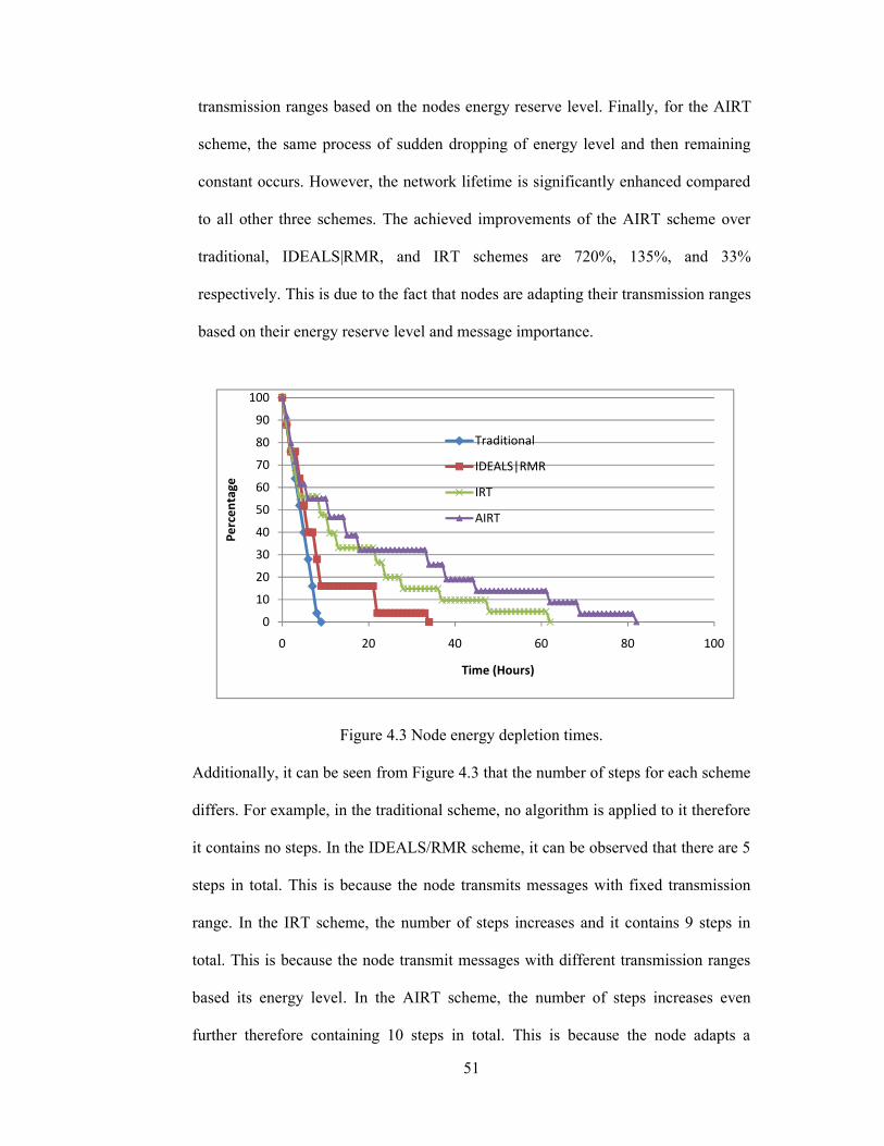
51
transmission ranges based on the nodes energy reserve level. Finally, for the AIRT
scheme, the same process of sudden dropping of energy level and then remaining
constant occurs. However, the network lifetime is significantly enhanced compared
to all other three schemes. The achieved improvements of the AIRT scheme over
traditional, IDEALS|RMR, and IRT schemes are 720%, 135%, and 33%
respectively. This is due to the fact that nodes are adapting their transmission ranges
based on their energy reserve level and message importance.
Figure 4.3 Node energy depletion times.
Additionally, it can be seen from Figure 4.3 that the number of steps for each scheme
differs. For example, in the traditional scheme, no algorithm is applied to it therefore
it contains no steps. In the IDEALS/RMR scheme, it can be observed that there are 5
steps in total. This is because the node transmits messages with fixed transmission
range. In the IRT scheme, the number of steps increases and it contains 9 steps in
total. This is because the node transmit messages with different transmission ranges
based its energy level. In the AIRT scheme, the number of steps increases even
further therefore containing 10 steps in total. This is because the node adapts a
0
10
20
30
40
50
60
70
80
90
100
0 20 40 60 80 100
Perc
enta
ge
Time (Hours)
Traditional
IDEALS|RMR
IRT
AIRT

52
suitable transmission range based on both the importance of the message and its
energy reserve level. We can say for a fact that the number of steps increased with
increase in the lifetime of the sensor nodes.
(2) Network connectivity: Network connectivity is defined as the measure of the
capability of any sensor node in the network to transmit message to the sink node
successfully. When all sensor nodes successfully transmit message to the sink node,
then the network is 100% connected. However if the network is 50% connected, then
only half of the nodes can successfully transmit a message to the sink node [31].
Figure 4.4 shows that the connectivity of the Traditional scheme is completely lost
after around 9 hrs. Figure 4.5 shows the connectivity of the IDEALS|RMR scheme. It
is clear from the figure that this scheme extends the network lifetime and hence
improves the network connectivity. The network lifetime for the most trivial message
(MP5) is lost after around 4hrs (therefore no message of MP5 importance can reach
the sink node after 4hrs) while it is connected for about 76%. However the network
is still around 80% connected for the most important message (MP1) for 34 hrs. This
is because the messages are not transmitted every 5 minutes as in the traditional
scheme. Figure 4.6 shows the performance of the IRT scheme. As it can be seen
from the figure, IRT manages to extend the network lifetime almost twice that of the
IDEALS/RMR scheme. This is because of the adjustment of transmission range
based on nodes energy level. Additionally, network lifetime for the most trivial
message is lost after around 13hrs while it is connected for about 76%. However the
network is 79.6% connected for the most important message for 63hrs. Finally,
Figure 4.7 shows the connectivity of the proposed AIRT scheme. It is obvious that
AIRT scheme outperforms all other schemes as it has the longest network lifetime
and maximum connectivity. It is interesting to note that AIRT extends the network
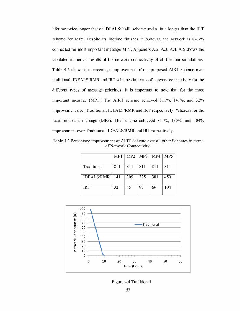
53
lifetime twice longer that of IDEALS/RMR scheme and a little longer than the IRT
scheme for MP5. Despite its lifetime finishes in 83hours, the network is 84.7%
connected for most important message MP1. Appendix A.2, A.3, A.4, A.5 shows the
tabulated numerical results of the network connectivity of all the four simulations.
Table 4.2 shows the percentage improvement of our proposed AIRT scheme over
traditional, IDEALS/RMR and IRT schemes in terms of network connectivity for the
different types of message priorities. It is important to note that for the most
important message (MP1). The AIRT scheme achieved 811%, 141%, and 32%
improvement over Traditional, IDEALS/RMR and IRT respectively. Whereas for the
least important message (MP5). The scheme achieved 811%, 450%, and 104%
improvement over Traditional, IDEALS/RMR and IRT respectively.
Table 4.2 Percentage improvement of AIRT Scheme over all other Schemes in termsof Network Connectivity.
MP1 MP2 MP3 MP4 MP5
Traditional 811 811 811 811 811
IDEALS/RMR 141 209 375 381 450
IRT 32 45 97 69 104
Figure 4.4 Traditional
0102030405060708090
100
0 10 20 30 40 50 60
Net
wor
k Co
nnec
tivity
(%)
Time (Hours)
Traditional
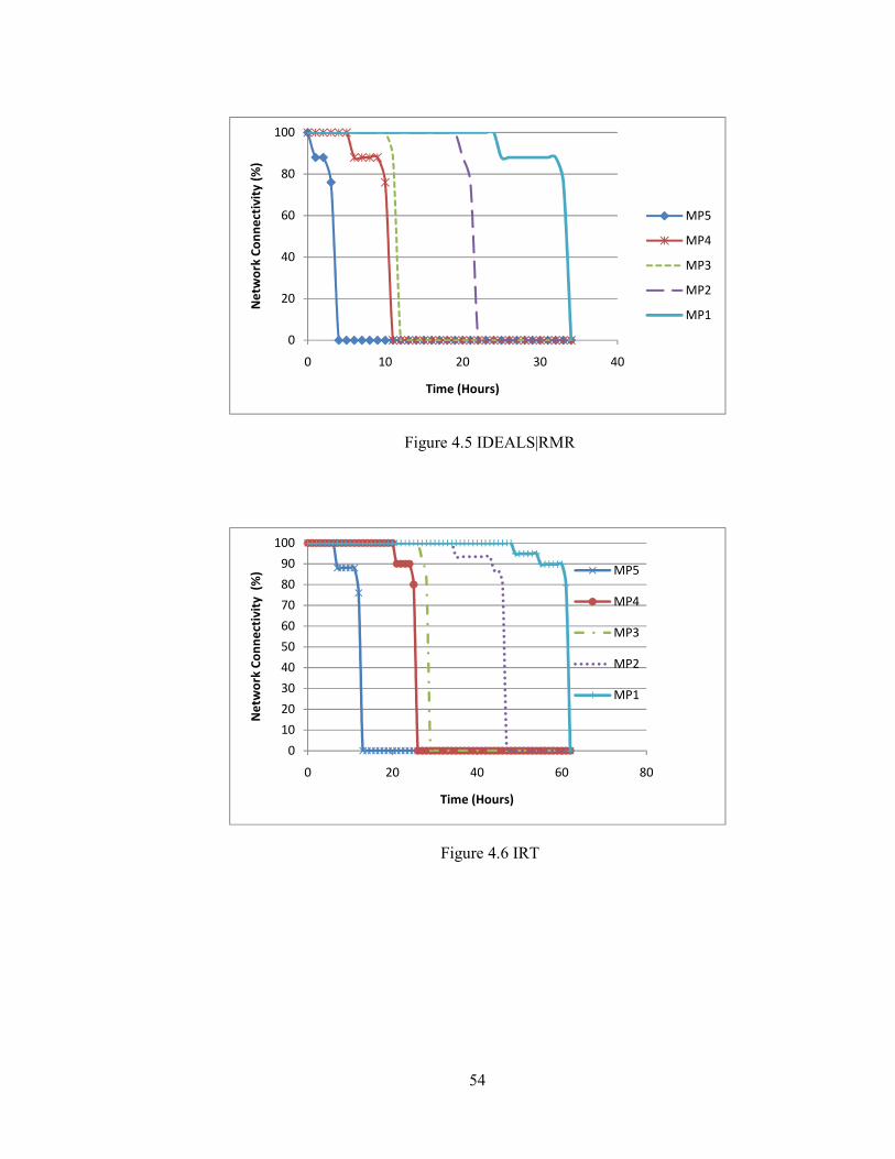
54
Figure 4.5 IDEALS|RMR
Figure 4.6 IRT
0
20
40
60
80
100
0 10 20 30 40
Net
wor
k Co
nnec
tivity
(%)
Time (Hours)
MP5
MP4
MP3
MP2
MP1
0102030405060708090
100
0 20 40 60 80
Net
wor
k Co
nnec
tivity
(%
)
Time (Hours)
MP5
MP4
MP3
MP2
MP1
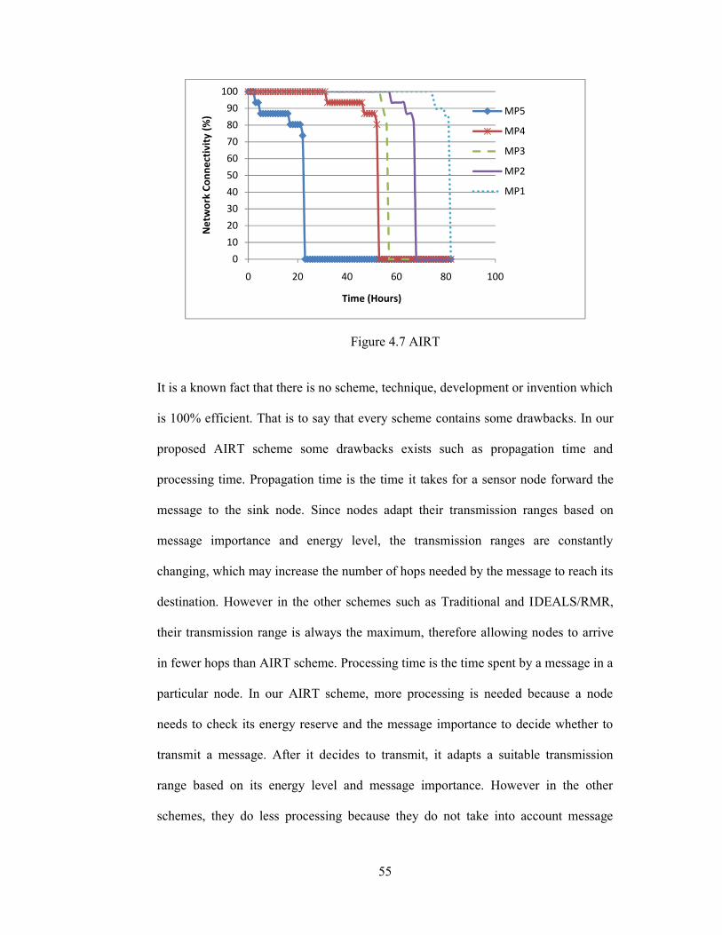
55
Figure 4.7 AIRT
It is a known fact that there is no scheme, technique, development or invention which
is 100% efficient. That is to say that every scheme contains some drawbacks. In our
proposed AIRT scheme some drawbacks exists such as propagation time and
processing time. Propagation time is the time it takes for a sensor node forward the
message to the sink node. Since nodes adapt their transmission ranges based on
message importance and energy level, the transmission ranges are constantly
changing, which may increase the number of hops needed by the message to reach its
destination. However in the other schemes such as Traditional and IDEALS/RMR,
their transmission range is always the maximum, therefore allowing nodes to arrive
in fewer hops than AIRT scheme. Processing time is the time spent by a message in a
particular node. In our AIRT scheme, more processing is needed because a node
needs to check its energy reserve and the message importance to decide whether to
transmit a message. After it decides to transmit, it adapts a suitable transmission
range based on its energy level and message importance. However in the other
schemes, they do less processing because they do not take into account message
0102030405060708090
100
0 20 40 60 80 100
Net
wor
k Co
nnec
tivity
(%)
Time (Hours)
MP5
MP4
MP3
MP2
MP1

56
importance and energy level to decide whether to transmit a message and the range
to transmit the message with.
4.4 Discussion
This chapter has presented the simulation algorithm for the AIRT scheme proposed
in this thesis. It provides the simulation results of a WSN environment using the
AIRT scheme and compares these results to other similar energy saving schemes. It
is seen that traditional case which did not use any power saving method, had the
shortest lifetime. When the IDEALS/RMR scheme was simulated, it showed a
considerable extension in network lifetime by extending the lifetime of high priority
messages and ignoring low priority messages. Similarly, IRT and AIRT which show
a considerable increase in network lifetime compared to IDEALDS/RMR extend
their lifetime by dropping low priority messages and extending lifetime of high
priority messages. The difference between IRT and AIRT is that the former adjusts it
transmission range based on nodes energy resource only, while the later extends it
based on energy resource and message importance. For that reason, AIRT is seen as
the best power saving technique compared to other three techniques as was
illustrated in the simulation results. The complete source codes of all the four energy
management schemes were provided in appendix B.
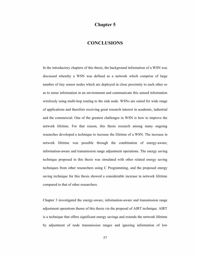
57
Chapter 5
CONCLUSIONS
In the introductory chapters of this thesis, the background information of a WSN was
discussed whereby a WSN was defined as a network which comprise of large
number of tiny sensor nodes which are deployed in close proximity to each other so
as to sense information in an environment and communicate this sensed information
wirelessly using multi-hop routing to the sink node. WSNs are suited for wide range
of applications and therefore receiving great research interest in academic, industrial
and the commercial. One of the greatest challenges in WSN is how to improve the
network lifetime. For that reason, this thesis research among many ongoing
researches developed a technique to increase the lifetime of a WSN. The increase in
network lifetime was possible through the combination of energy-aware,
information-aware and transmission range adjustment operations. The energy saving
technique proposed in this thesis was simulated with other related energy saving
techniques from other researchers using C Programming, and the proposed energy
saving technique for this thesis showed a considerable increase in network lifetime
compared to that of other researchers.
Chapter 3 investigated the energy-aware, information-aware and transmission range
adjustment operations theme of this thesis via the proposal of AIRT technique. AIRT
is a technique that offers significant energy savings and extends the network lifetime
by adjustment of node transmission ranges and ignoring information of low
58
importance. The extension in network life was possible through the combination of
RMR (for controlling information sensing), IDEAL (for controlling information
propagation) and TRA (adjusting of communication range).
Chapter 4 presents the simulation results obtained using C Programming Language to
evaluate the proposed AIRT algorithm of this thesis. The results show a considerable
increase in network lifetime of high importance messages compared to similar
researches of other researchers. Besides extending the network lifetime which was
the primary goal of this thesis, network connectivity was also enhanced compared to
that of other researchers.
This thesis has highlighted the benefit of combining various power saving techniques
(such as information control, energy control and transmission range control) to
improve network lifetime.
The most important finding in this thesis is the development of the AIRT scheme. It
is important to note that for the node energy depletion time performance metric. The
achieved improvements of the AIRT scheme over traditional, IDEALS|RMR, and
IRT schemes are 720%, 135%, and 33% respectively. Additionally, for the network
connectivity performance metric. The AIRT scheme achieved 811%, 141%, and 32%
improvement over Traditional, IDEALS/RMR, and IRT schemes respectively for the
most important message (MP1). Whereas the scheme achieved 811%, 450%, and
104% improvement over Traditional, IDEALS/RMR and IRT respectively for the
least important message (MP5). This advantage of the AIRT scheme over other
related energy saving schemes is due to the fact that nodes are adapting their
transmission ranges based on their energy reserve level and message importance.
59
Despite the achieved improvements of our proposed AIRT scheme, the scheme does
not escape from some drawbacks such as propagation time, and processing time.
The drawbacks mentioned do not have much effect on our scheme. This is because
our scheme is intended for networks with few number of sensor nodes, as wireless
sensor networks are application dependant.
Using the AIRT scheme proposed and simulated in this thesis a considerable increase
in network lifetime and connectivity is achieved. For that reason, the research aims
mentioned in section 1.1 were successfully fulfilled.
Future works
As WSNs are continuously been popular, the need for further research is to extend
the network lifetime is required. Example of possible further research could be:
- To use RMR, IDEALS and TRA operations separately in other researches in
other to improve the network lifetime.
- The AIRT could be employed to use the forth power saving technique which
is the duty cycle operation (alternating between sleep and active mode) to
extend the network lifetime.
- Fuzzy logic may be added to the RMR operation of AIRT in deciding the
importance of a message.
- Weights can be given to message types and
- Studying of more than five levels may be considered.
60
REFERENCES
[1] Akyildiz I.F., Su W., Sankarasubramaniam Y., and Cayirci E., "A survey on
sensor networks," Communications Magazine, vol. 40, pp. 102-114, Aug. 2002.
[2] Merrett, G. V. “Energy- and Information- Managed Wireless Sensor Networks:
Modelling and Simulation”. PhD thesis, University of Southampton, (2009).
[3] [Merrett, G.V., B.M. A`l-Hashimi, N.M., White, N.R. Harris, “Information
managed wireless sensor networks with energy aware nodes,” in: Proceedings of the
2005 NSTI Nanotechnology Conference and Trade Show (Nano Tech’05), Anaheim,
CA, pp. 367-370, (2005).
[4] Cardei, M.; Du, D.Z. “Improving wireless sensor network lifetime through power
aware organization,” Wirel. Netw. , 11, 333-340, (2005).
[5] Carle, J.; Simplot, D. “Energy-efficient area monitoring by sensor networks,”
IEEE Comput. 37, 40 - 46, (2004).
[6] Cardei, M.; Wu, J.; Lu, M. “Improving network lifetime using sensors with
adjustable sensing ranges,” Int. J. Sensor Networks, 1, 41-49, (2006).
[7] Wu, J.; Dai, F. “Virtual backbone construction in MANETs using adjustable
transmission ranges,” IEEE Trans. Mob. Comput., 5, 1188-1200, (2006).
61
[8] Rabaey J.M., Ammer M.J., Da Silva J.L., Jr. et al., "PicoRadio supports ad hoc
ultra-low power wireless networking," Computer, vol. 33, pp. 42-48, Jul. 2000.
[9] Dierdonck N.V., "Wireless Standards Demystified," GreenPeak Technologies,
20080114 Standards overview.doc, Feb. 2008.
[10] Towson, "Ubiquitous Wireless Sensor Networks: An Introduction," presented at
WSN Training: Intro to Wireless Sensor Networks, Nov. 2005.
[11] Akyildiz I.F., Su W., Sankarasubramaniam Y., and Cayirci E., "A survey on
sensor networks," Communications Magazine, vol. 40, pp. 102-114, Aug. 2002.
[12] V. Raghunathan, C. Schurgers, S. Park, and M.B. Srivastava, "Energy-aware
wireless microsensor networks," Signal Processing Magazine, vol. 19, pp. 40-50,
Mar. 2002.
[13] Giuseppe A., Marco C., Mario D.F., Andrea P.,” Energy conservation in
wireless sensor networks: A survey,” Ad Hoc Networks vol. 7, pp. 537–568, (2009).
[14] Jennifer Y., Biswanath M., Dipak G., “Wireless sensor network survey,”
Computer Networks vol. 52, pp. 2292–2330, (2008).
[15] http://en.wikipedia.org/wiki/Wireless_sensor_network#cite_note-Tiwari-3; last
accessed March 15, 2011.
62
[16] Junqi Z., Vijay V., “Wireless sensor network key management survey and
taxonomy,” Journal of Network and Computer Applications vol. 33, pp. 63–75
(2010).
[17] Arampatzis T., Lygeros J., and Manesis S., "A survey of applications of wireless
sensors and wireless sensor networks," in Proc. Mediterranean Conf. Control and
Automation, Limassol, Cyprus, pp. 719-724, Jun. 2005.
[18] OFCOM, "Technology Trends Workshop Report," London, Dec. 2007.
[19] Deb B., Bhatnagar S., and B. Nath, "Information Assurance in Sensor
Networks," in Proc. 2ndACM Int'l Workshop Wireless Sensor networks and
Applications (WSNA'03), San Diego, CA, United States, pp. 160-168, Sep 2003.
[20] Jennifer Y., Biswanath M., Dipak G., “Wireless sensor network survey,”
Computer Networks vol. 52, pp. 2292–2330, (2008).
[21] Min R., Bhardwaj M., S.H., C. et al., "Low-power wireless sensor networks," in
Proc. 14th Int'l Conf. VLSI Design, pp. 205-210, Jan. 2001.
[22] Chandrakasan A., Min R., Bhardwaj M. et al., "Power Aware Wireless
Microsensor Systems," in Proc. Solid-State Device Research Conference, 2002.
Proceeding of the 32nd European, pp. 37-44, Sep. 2002.
63
[23] Dutta P.K. and Culler D.E., "System software techniques for low-power
operation in wirelesssensor networks," in Proc. Int'l Conf. Computer Aided Design
(ICCAD'05), San Jose, CA, USA, pp. 925-32, Nov. 2005.
[24] P.H. Chou and C. Park, "Energy-efficient platform designs for real-world
wireless sensing applications," in Proc. Int'l Conf. Computer Aided Design
(ICCAD'05), San Jose, CA, USA, pp. 913-20, Nov. 2005.
[25] Mingming, L., Jie, W., Mihaela, C., Minglu, L., “Energy-Efficient Connected
Coverage of Discrete Targets in Wireless Sensor Networks,” International Journal of
Ad Hoc and Ubiquitous Computing, vol. 4, pp. 137 - 147, (2009).
[26] Starner T., and Paradiso J.A., "Human Generated Power for Mobile
Electronics," in Low Power Electronics Design, vol. Chapter 35, C. Piguet, Ed.: CRC
Press, pp. 1-35, (2004).
[27] Atay O., Cem E.,” WCOT: A utility based lifetime metric for wireless sensor
networks,” Computer Communications, vol. 32, pp. 409–418, (2009).
[28] Delin K., and Jackson S., "The Sensor Web: A New Instrument Concept," in
Proc. SPIE Symp. Integrated Optics, San Jose, CA, Jan. 2001.
[29] Cianci C.M., Trifa V., and Martinoli A., "Threshold-based algorithms for
power-aware load balancing in sensor networks," in Proc. Swarm Intelligence
Symposium, Pasadena, CA, pp. 349-56, Jun. 2005.
64
[30] Cerpa A., and Estrin D., "ASCENT: Adaptive Self-Configuring sEnsor
Networks Topologies," in Proc. 21st Conf. IEEE Computer and Communications
Societies (INFOCOM'02), vol. 3, pp. 1278-1287, Jun. 2002.
[31] Hao L., Huifang M., Li L., Lian L., Heping Z., “Energy conservation in
wireless sensor networks and connectivity of graphs,” Theoretical Computer Science,
Volume 393 Issue 1-3, Mar. 2008.
[32] Chen D., and Varshney P., K., "QoS support in wireless sensor networks: A
survey," in Proc. Int'l Conf. Wireless Networks, Las Vegas, NV, vol. 1, pp. 227-233.
[33] Durresi A., "Architectures for Heterogeneous Wireless Sensor Networks Invited
Paper," inProc. 16th IEEE Int'l Symp Personal, Indoor and Mobile Radio
Communications (PIMRC'05), vol. 2, pp. 1289-1296, Sep. 2005.
[34] Bonnet P., Gehrke J., and Seshadri P., "Querying the physical world," IEEE
Personal Communications, vol. 7, pp. 10-15, Oct. 2000.
[35] Bonnet P., Gehrke J., and Seshadri P., "Querying the physical world," IEEE
PersonalCommunications, vol. 7, pp. 10-15, Oct. 2000.
[36] Yao Y., and Gehrke J., "The Cougar approach to in-network query processing in
sensor networks," SIGMOD Record, vol. 31, pp. 9-18, Sep. 2002.
65
[37] Manjeshwar A., and Agrawal D., P., "TEEN: a routing protocol for enhanced
efficiency in wireless sensor networks," in Proc. 15th Int'l Parallel and Distributed
Processing Symp. (IPDPS'01), pp. 2009-2015, Apr. 2001.
[38] Merrett G., V., Harris N., R., Al-Hashimi B., M., and White N., M., “Energy
Managed Reporting for Wireless Sensor Networks,” in Sensors and Actuators A:
Physical, vol. 142, pp. 379-389, 2008.
[39] The Distance Formula, http://www.purplemath.com/modules/distform.htm.
[40] Wenz M., and Worn H., "Event-based Production Rules for Data Aggregation in
Wireless Sensor Networks," in Proc. IEEE Int'l Conf. Multisensor Fusion and
Integration for Intelligent Systems, pp. 59-64, Sep. 2006.
[41] Cardei M., Thai M., Li Y., and Wu W., “Energy-Efficient Target Coverage in
Wireless Sensor Networks,” IEEE INFOCOM 2005, Mar. 2005.
[42] Cardei M., Wu J., Lu M., and Pervaiz M., “Maximum Network Lifetime in
Wireless Sensor Networks with Adjustable Sensing Ranges,” IEEE WiMob2005,
Aug. 2005.
[43] "Information technology - Open Systems Interconnection - Basic Reference
Model: The Basic Model", 1994.
[44] Meyer D., and Zobrist G., "TCP/IP versus OSI," IEEE Potentials, vol. 9, pp. 16-
19, Feb. 1990.
66
[45] Kolla S., Border D., and Mayer E., "Fieldbus networks for control system
implementations," in Proc. Electrical Insulation Conf. & Electrical Manufacturing &
Coil Winding Technology Conf., pp. 493-498, Sep. 2003.
[46] ZigBee Alliance, "ZigBee Specification Document 053474r17", 2007.
[47] Demirkol I., Ersoy C., and Alagoz F., "MAC protocols for wireless sensor
networks: a survey," IEEE Communications Magazine, vol. 44, pp. 115-121, Apr.
2006.
[48] Al-Karaki J., N., and Kamal A., E., "Routing techniques in wireless sensor
networks: a survey," Wireless Communications, vol. 11, pp. 6-28, Dec. 2004.
[49] Abdullahi, A.I., Muhammed, S., “Energy-Aware Transmission Scheme for
Wireless Sensor Networks,” WiMo, Ankara, Turkey, Mar. 2011.
[50] The Network Simulator - ns2, www.isi.edu/nsnam/ns; last accessed Mar. 2011.
[51] Heinzelman W.R., Chandrakasan A., and Balakrishnan H., "Energy-efficient
communication protocol for wireless microsensor networks," in Proc. 33rd Int'l
Conf. System Sciences, Hawaii, Jan. 2000.

67
APPENDIX

68
Appendix A: Simulation Raw Data
Table A.1 Energy depletion times of Traditional, IDEALS/RMR, IRT and AIRT
simulations
Time Traditional IDEALS/RMR IRT AIRT(Hours) (Joules) (Joules) (Joules) (Joules)
0 100 100 100 1001 88 87.999702 87.999702 91.8131792 76 75.999405 75.999405 79.8128813 64 75.999405 65.996712 71.626064 52 63.999104 55.994019 61.6233675 39.99 51.998802 55.994019 61.6233676 27.99 39.998501 55.994019 55.0706757 15.99 39.998501 55.994019 55.0706758 3.99 27.998201 55.994019 55.0706759 0 15.997901 47.807198 55.070374
10 15.997901 47.807198 55.07037411 15.997901 39.620377 46.88355312 15.997901 39.620377 46.88325113 15.997901 33.067684 46.8829514 15.997901 33.067684 46.88264815 15.997901 33.067684 38.69582716 15.997901 33.067684 38.69582717 15.997901 33.067684 38.69582718 15.997901 33.067684 32.14313519 15.997901 33.067684 32.14313520 15.997901 33.067684 32.14313521 15.997901 33.067684 32.14313522 3.997601 26.514994 32.14313523 3.997601 26.514994 32.14313524 3.997601 19.962303 32.14313525 3.997601 19.962303 32.14313526 3.997601 19.962303 32.14313527 3.997601 19.962303 32.14313528 3.997601 14.862002 32.14313529 3.997601 14.862002 32.14313530 3.997601 14.862002 32.14313531 3.997601 14.862002 32.14313532 3.997601 14.862002 32.14313533 3.997601 14.862002 32.143135

69
Table A.1 (continued) Energy depletion times of Traditional, IDEALS/RMR, IRT
and AIRT simulations
34 0 14.862002 25.59044535 14.862002 25.59044536 14.862002 25.59044537 9.761702 25.59044538 9.761702 19.03775439 9.761702 19.03775440 9.761702 19.03775441 9.761702 19.03775442 9.761702 19.03775443 9.761702 19.03775444 9.761702 19.03775445 9.761702 13.93745346 9.761702 13.93745347 9.761702 13.93745348 4.661401 13.93745349 4.661401 13.93745350 4.661401 13.93745351 4.661401 13.93745352 4.661401 13.93745353 4.661401 13.93745354 4.661401 13.93745355 4.661401 13.93745356 4.661401 13.93745357 4.661401 13.93745358 4.661401 13.93745359 4.661401 13.93745360 4.661401 13.93745361 4.661401 13.93745362 0 8.83715263 8.83715264 8.83715265 8.83715266 8.83715267 8.83715268 8.837152

70
Table A.1 (continued) Energy depletion times of Traditional, IDEALS/RMR, IRT
and AIRT simulations
69 3.73685270 3.73685271 3.73685272 3.73685273 3.73685274 3.73685275 3.73685276 3.73685277 3.73685278 3.73685279 3.73685280 3.73685281 3.73685282 0
Table A.2 Network connectivity for Traditional simulation
Time Traditional(Hours) (Joules)
0 1001 882 763 644 525 39.996 27.997 15.998 3.999 0

71
Table A.3 Network connectivity for IDEALS/RMR simulation
Time(Hour) MP5 MP4 MP3 MP2 MP1
0 100 100 100 100 1001 87.999702 100 100 100 1002 87.999702 100 100 100 1003 75.999405 100 100 100 1004 0 100 100 100 1005 0 100 100 100 1006 0 87.999702 100 100 1007 0 87.999702 100 100 1008 0 87.999702 100 100 1009 0 87.999702 100 100 100
10 0 75.999405 100 100 10011 0 0 87.999702 100 10012 0 0 0 100 10013 0 0 0 100 10014 0 0 0 100 10015 0 0 0 100 10016 0 0 0 100 10017 0 0 0 100 10018 0 0 0 100 10019 0 0 0 100 10020 0 0 0 87.999702 10021 0 0 0 75.999405 10022 0 0 0 0 10023 0 0 0 0 10024 0 0 0 0 10025 0 0 0 0 87.99970226 0 0 0 0 87.99970227 0 0 0 0 87.99970228 0 0 0 0 87.99970229 0 0 0 0 87.99970230 0 0 0 0 87.99970231 0 0 0 0 87.99970232 0 0 0 0 87.99970233 0 0 0 0 75.99940534 0 0 0 0 0

72
Table A.4 Network connectivity for IRT simulation
Time(Hour) MP5 MP4 MP3 MP2 MP1
0 100 100 100 100 1001 100 100 100 100 1002 100 100 100 100 1003 100 100 100 100 1004 100 100 100 100 1005 100 100 100 100 1006 100 100 100 100 1007 87.999702 100 100 100 1008 87.999702 100 100 100 1009 87.999702 100 100 100 100
10 87.999702 100 100 100 10011 87.999702 100 100 100 10012 75.999405 100 100 100 10013 0 100 100 100 10014 0 100 100 100 10015 0 100 100 100 10016 0 100 100 100 10017 0 100 100 100 10018 0 100 100 100 10019 0 100 100 100 10020 0 100 100 100 10021 0 89.997307 100 100 10022 0 89.997307 100 100 10023 0 89.997307 100 100 10024 0 89.997307 100 100 10025 0 79.994614 100 100 10026 0 0 100 100 10027 0 0 91.813179 100 10028 0 0 83.626358 100 10029 0 0 0 100 10030 0 0 0 100 10031 0 0 0 100 10032 0 0 0 100 10033 0 0 0 100 10034 0 0 0 100 10035 0 0 0 93.447311 100
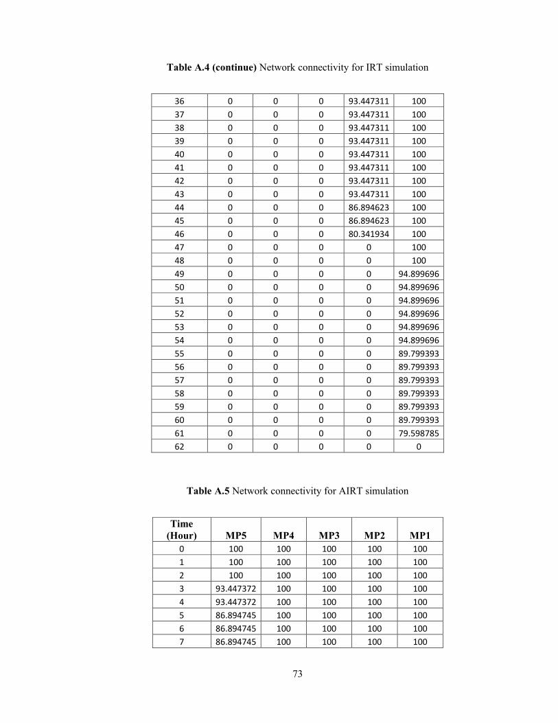
73
Table A.4 (continue) Network connectivity for IRT simulation
36 0 0 0 93.447311 10037 0 0 0 93.447311 10038 0 0 0 93.447311 10039 0 0 0 93.447311 10040 0 0 0 93.447311 10041 0 0 0 93.447311 10042 0 0 0 93.447311 10043 0 0 0 93.447311 10044 0 0 0 86.894623 10045 0 0 0 86.894623 10046 0 0 0 80.341934 10047 0 0 0 0 10048 0 0 0 0 10049 0 0 0 0 94.89969650 0 0 0 0 94.89969651 0 0 0 0 94.89969652 0 0 0 0 94.89969653 0 0 0 0 94.89969654 0 0 0 0 94.89969655 0 0 0 0 89.79939356 0 0 0 0 89.79939357 0 0 0 0 89.79939358 0 0 0 0 89.79939359 0 0 0 0 89.79939360 0 0 0 0 89.79939361 0 0 0 0 79.59878562 0 0 0 0 0
Table A.5 Network connectivity for AIRT simulation
Time(Hour) MP5 MP4 MP3 MP2 MP1
0 100 100 100 100 1001 100 100 100 100 1002 100 100 100 100 1003 93.447372 100 100 100 1004 93.447372 100 100 100 1005 86.894745 100 100 100 1006 86.894745 100 100 100 1007 86.894745 100 100 100 100

74
Table A.5 (continue) Network connectivity for AIRT simulation
8 86.894745 100 100 100 1009 86.894745 100 100 100 100
10 86.894745 100 100 100 10011 86.894745 100 100 100 10012 86.894745 100 100 100 10013 86.894745 100 100 100 10014 86.894745 100 100 100 10015 86.894745 100 100 100 10016 86.894745 100 100 100 10017 80.342117 100 100 100 10018 80.342117 100 100 100 10019 80.342117 100 100 100 10020 80.342117 100 100 100 10021 80.342117 100 100 100 10022 73.78949 100 100 100 10023 0 100 100 100 10024 0 100 100 100 10025 0 100 100 100 10026 0 100 100 100 10027 0 100 100 100 10028 0 100 100 100 10029 0 100 100 100 10030 0 100 100 100 10031 0 100 100 100 10032 0 93.447372 100 100 10033 0 93.447372 100 100 10034 0 93.447372 100 100 10035 0 93.447372 100 100 10036 0 93.447372 100 100 10037 0 93.447372 100 100 10038 0 93.447372 100 100 10039 0 93.447372 100 100 10040 0 93.447372 100 100 10041 0 93.447372 100 100 10042 0 93.447372 100 100 10043 0 93.447372 100 100 10044 0 93.447372 100 100 10045 0 93.447372 100 100 10046 0 93.447372 100 100 10047 0 86.894745 100 100 100

75
Table A.5 (continue) Network connectivity for AIRT simulation
48 0 86.894745 100 100 10049 0 86.894745 100 100 10050 0 86.894745 100 100 10051 0 86.894745 100 100 10052 0 80.342117 100 100 10053 0 0 100 100 10054 0 0 93.447372 100 10055 0 0 86.894745 100 10056 0 0 80.342117 100 10057 0 0 0 100 10058 0 0 0 93.447372 10059 0 0 0 93.447372 10060 0 0 0 93.447372 10061 0 0 0 93.447372 10062 0 0 0 93.447372 10063 0 0 0 93.447372 10064 0 0 0 86.894745 10065 0 0 0 86.894745 10066 0 0 0 86.894745 10067 0 0 0 80.342117 10068 0 0 0 0 10069 0 0 0 0 10070 0 0 0 0 10071 0 0 0 0 10072 0 0 0 0 10073 0 0 0 0 10074 0 0 0 0 10075 0 0 0 0 94.8997876 0 0 0 0 89.79956177 0 0 0 0 89.79956178 0 0 0 0 89.79956179 0 0 0 0 89.79956180 0 0 0 0 84.69934181 0 0 0 0 84.69934182 0 0 0 0 0

76
Appendix B: Source Codes which are used in the performance measurement
Source Code for Energy Depletion Times simulation of Traditional algorithm
Abdullahi Ibrahim ABDU
Department of Computer Engineering
Eastern Mediterranean University
/* The coordinates of all the sensor nodes must be saved in a file*/
#include<stdio.h>
#include<stdlib.h>
#include<time.h>
#define SENS 20 /* the number of nodes */
#define RADIUS 20 /* radius of each node */
#define GEN 9 /* number of generations */
struct Sensor{
int id; /* identity of this sensor */
double battery; /* the energy of this sensor, i.e. 100 J*/
int x_coord,y_coord; /* x and y coordinates of this sensor */
int reachable_sensors[SENS - 1]; /* the maximum number of nodes that arein radius of this sensor */
int data; /* information that is sensed by this sensor */
int sent; /* whether information was sent by this sensor */
double transmission_range[SENS - 1];
};
#include "init.h" /* containing functions for initializing the sensors nodes with *//* coordinates and finding sensor nodes in the 20meters radius */
#include "send_data.h" /* contains a function for sending sensed data */
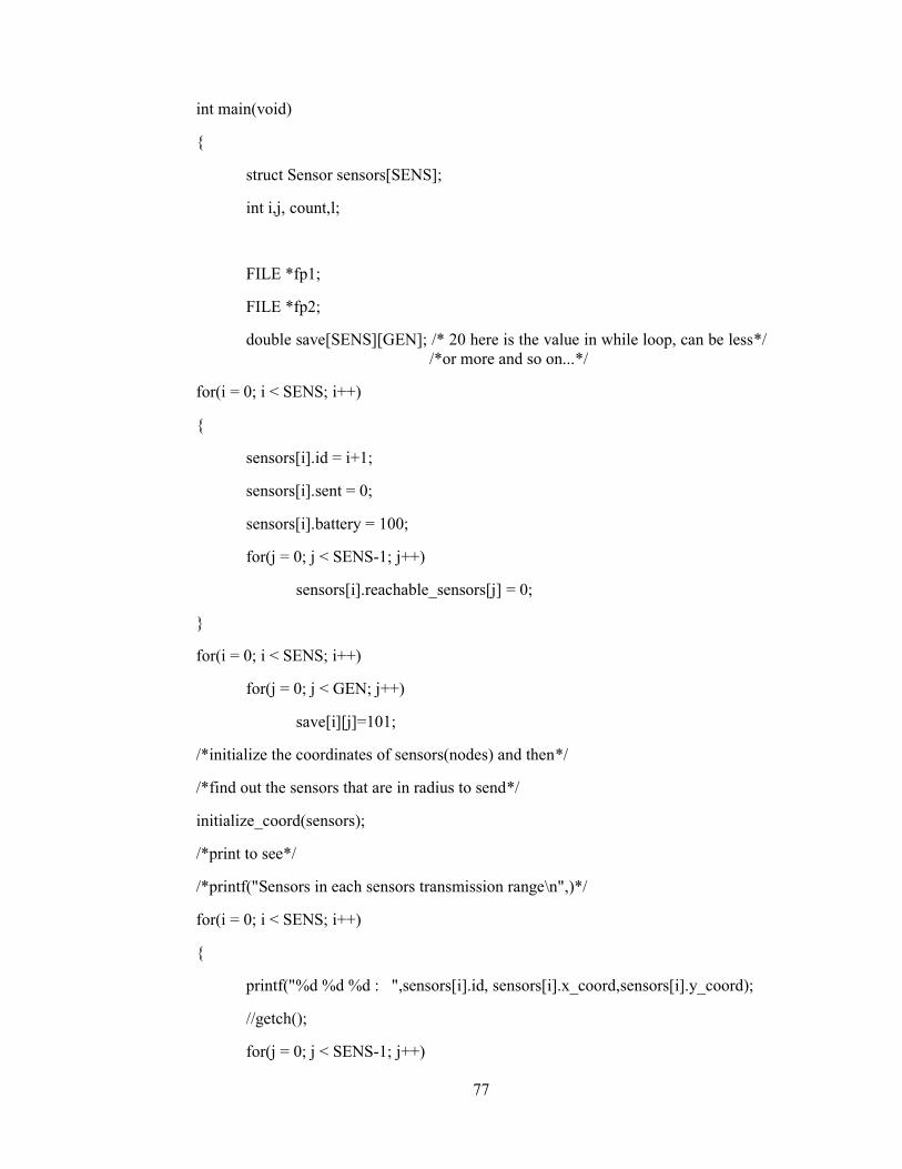
77
int main(void)
{
struct Sensor sensors[SENS];
int i,j, count,l;
FILE *fp1;
FILE *fp2;
double save[SENS][GEN]; /* 20 here is the value in while loop, can be less*//*or more and so on...*/
for(i = 0; i < SENS; i++)
{
sensors[i].id = i+1;
sensors[i].sent = 0;
sensors[i].battery = 100;
for(j = 0; j < SENS-1; j++)
sensors[i].reachable_sensors[j] = 0;
}
for(i = 0; i < SENS; i++)
for(j = 0; j < GEN; j++)
save[i][j]=101;
/*initialize the coordinates of sensors(nodes) and then*/
/*find out the sensors that are in radius to send*/
initialize_coord(sensors);
/*print to see*/
/*printf("Sensors in each sensors transmission range\n",)*/
for(i = 0; i < SENS; i++)
{
printf("%d %d %d : ",sensors[i].id, sensors[i].x_coord,sensors[i].y_coord);
//getch();
for(j = 0; j < SENS-1; j++)
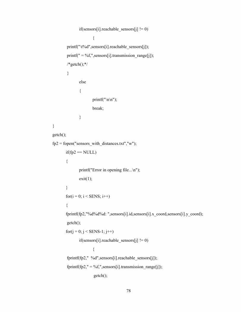
78
if(sensors[i].reachable_sensors[j] != 0)
{
printf("\t%d",sensors[i].reachable_sensors[j]);
printf(" = %f,",sensors[i].transmission_range[j]);
/*getch();*/
}
else
{
printf("\n\n");
break;
}
}
getch();
fp2 = fopen("sensors_with_distances.txt","w");
if(fp2 == NULL)
{
printf("Error in opening file...\n");
exit(1);
}
for(i = 0; i < SENS; i++)
{
fprintf(fp2,"%d%d%d: ",sensors[i].id,sensors[i].x_coord,sensors[i].y_coord);
getch();
for(j = 0; j < SENS-1; j++)
if(sensors[i].reachable_sensors[j] != 0)
{
fprintf(fp2," %d",sensors[i].reachable_sensors[j]);
fprintf(fp2," = %f,",sensors[i].transmission_range[j]);
getch();
79
}
else
{
fprintf(fp2,"\n\n");
break;
}
}
fclose(fp2);
/*generate random data*/
fp1 = fopen("TRADITIONAL-CASE-RESULTS.txt","w");
if(fp1 == NULL)
{
printf("Error in opening file...\n");
exit(1);
}
count = 0;
srand(time(NULL));
while (count<GEN)
{
for(i=0;i<SENS;i++)
{
if(sensors[i].battery>0)
{
sensors[i].data = 25+rand()%50;
send_data(sensors,sensors[i].id,sensors[i].data);
}
for(l=0;l<SENS;l++)
sensors[l].sent = 0;
for(l=0;l<SENS;l++)
80
save[l][count] = sensors[l].battery;
}
count++;
}
for(i=0;i<SENS;i++)
{
if(save[i][0] != 101.0)
{
fprintf(fp1,"100\t");
for(j=0;j<GEN;j++)
fprintf(fp1,"%.2lf\t",save[i][j]);
fprintf(fp1,"\n");
}
}
fclose(fp1);
for(i=0;i<SENS;i++)
{
{
printf("100\t");
for(j=0;j<GEN;j++)
printf("%.2lf\t",save[i][j]);
printf("\n");
}
}
getch();
return 0;
}
/****************************Init.h header file*************************/
81
#include<math.h>
void find_in_radius(struct Sensor ss[SENS]);
void initialize_coord(struct Sensor s[SENS]) /*creating a structure of 20 sensors*/
{
char c,c1;
int i;
FILE *fp;
fp = fopen("coordinates.txt","r");
if(fp == NULL)
{
printf("Error in opening file...\n");
exit(1);
}
for(i=0;i<SENS;i++)
{
fscanf(fp,"%d%c%d%c",&s[i].x_coord,&c,&s[i].y_coord,&c1 );/*intializing each of the sensors with the values in*/
}
fclose(fp);
find_in_radius(s);
}
void find_in_radius(struct Sensor ss[SENS])
{ int i,j,k,p;
int x1,y1,x2,y2,d;
double distance;
for(i = 0; i < SENS; i++)
{
k = 0;
p = 0;
x1 = ss[i].x_coord;
82
y1 = ss[i].y_coord;
for(j = 0; j < SENS; j++)
{
if(j==i) continue;
x2 = ss[j].x_coord;
y2 = ss[j].y_coord;
d = (x2-x1)*(x2-x1) + (y2-y1)*(y2-y1);
distance = sqrt(d);
if( distance <= RADIUS )
{
ss[i].reachable_sensors[k++] = ss[j].id;
ss[i].transmission_range[p++] = distance;
}
}
}
}
/*************************send_data.h header file**********************/
83
#include<math.h>
int Received = 0;
void send_data(struct Sensor s[SENS],int id, int data)
{
static int value = 0;
int j;
if(s[id-1].battery>0)
{
s[id-1].battery -= 0.0000003*1000 + 0.00003*1000*pow(RADIUS,2);
s[id-1].sent = 1;
for(j=0;j<SENS-1;j++)
{
if(s[id-1].reachable_sensors[j]!=0)
{
s[s[id-1].reachable_sensors[j]-1].battery -= 0.0000003*1000;
s[s[id-1].reachable_sensors[j]-1].data = data;
if(s[s[id-1].reachable_sensors[j]-1].id == 20)//if sink node received//the data...
{
Received = 1;
break;
}
}
}
}
if(Received == 0)
for(j=0;j<SENS-1;j++)
{
if(s[id-1].reachable_sensors[j]!=0 && s[id-1].sent != 1)
send_data(s, s[id-1].reachable_sensors[j], s[s[id-1].reachable_sensors[j]-1].data);

84
}
else
Received = 0;
}
//Source Codes for IREALS/RMR algorithm

85
//By, Abdullahi Ibrahim Abdu
/*****Energy depletion time source code for IDEALS/RMR algorithm******/
#include<stdio.h>
#include<stdlib.h>
#include<conio.h>
#include<time.h>
#include<math.h>
#define SENS 1
#define RADIUS 20
#define MAX 5
#define GEN 288
int main(void)
{
int node_id,PP,MP,TR;
int cnt = 0,i=0;
float min_dist,range_interval,tr[MAX];
float battery = 100.0;
float battery_buffer[GEN];
int mp5_sent=0,mp4_sent=0,mp3_sent=0,mp2_sent=0,mp1_sent=0;
int mp5_lost=0,mp4_lost=0,mp3_lost=0,mp2_lost=0,mp1_lost=0;
FILE *fp;
printf("ENTER SENSOR NODE ID: ");
scanf("%d",&node_id);
printf("\n");
for(int w=0;w<GEN;w++)
battery_buffer[w]=0;
srand(time(NULL));
86
while(battery>=0.0)
{
MP = 1+rand()%5;
if((battery<=100.0)&&(battery>=80.0))
{
PP=5;
if(MP==5) mp5_sent++;
if(MP==4) mp4_sent++;
if(MP==3) mp3_sent++;
if(MP==2) mp2_sent++;
if(MP==1) mp1_sent++;
if(PP>=MP)
{
battery-= 0.0000003*1000 + 0.00003*1000*pow(RADIUS,2);
battery_buffer[i] = battery;
cnt++;
i++;
continue;
}
}
if((battery<=80.0)&&(battery>=60.0))
{
PP=4;
if(MP==5) mp5_lost++;
if(MP==4) mp4_sent++;
if(MP==3) mp3_sent++;
if(MP==2) mp2_sent++;
if(MP==1) mp1_sent++;
if(PP>=MP)
87
{
battery-= 0.0000003*1000 + 0.00003*1000*pow(RADIUS,2);
battery_buffer[i] = battery;
cnt++;
i++;
continue;
}
battery_buffer[i] = battery;
cnt++;
i++;
continue;
}
if((battery<=60.0)&&(battery>=40.0))
{
PP=3;
if(MP==5) mp5_lost++;
if(MP==4) mp4_lost++;
if(MP==3) mp3_sent++;
if(MP==2) mp2_sent++;
if(MP==1) mp1_sent++;
if(PP>=MP)
{
battery-= 0.0000003*1000 + 0.00003*1000*pow(RADIUS,2);
battery_buffer[i] = battery;
cnt++;
i++;
continue;
}
battery_buffer[i] = battery;
88
cnt++;
i++;
continue;
}
if((battery<=40.0)&&(battery>=20.0))
{
PP=2;
if(MP==5) mp5_lost++;
if(MP==4) mp4_lost++;
if(MP==3) mp3_lost++;
if(MP==2) mp2_sent++;
if(MP==1) mp1_sent++;
if(PP>=MP)
{
battery-= 0.0000003*1000 + 0.00003*1000*pow(RADIUS,2);
battery_buffer[i] = battery;
cnt++;
i++;
continue;
}
battery_buffer[i] = battery;
cnt++;
i++;
continue;
}
if((battery<=20.0)&&(battery>=1.0))
{
PP=1;
if(MP==5) mp5_lost++;
89
if(MP==4) mp4_lost++;
if(MP==3) mp3_lost++;
if(MP==2) mp2_lost++;
if(MP==1) mp1_sent++;
if(PP>=MP)
{
battery-= 0.0000003*1000 + 0.00003*1000*pow(RADIUS,2);
battery_buffer[i] = battery;
cnt++;
i++;
continue;
}
battery_buffer[i] = battery;
cnt++;
i++;
continue;
}
}
printf("\n\n");
for(int p=0;p<cnt;p++)
printf("battery_buffer %d : %f\n",p+1,battery_buffer[p]);
printf("%d%d%d%d%d\n",mp5_sent,mp4_sent,mp3_sent,mp2_sent,mp1_sent);
printf("%d%d%d%d %d\n",mp5_lost,mp4_lost,mp3_lost,mp2_lost,mp1_lost);
printf("\n");
getch();
fp = fopen("IDEAL-RMR-lifetime.txt","w");
if(fp == NULL)
{
printf("Error in opening file...\n");

90
exit(1);
}
for(int p=0;p<cnt;p++)
fprintf(fp,"battery_buffer %d : %f\n",p+1,battery_buffer[p]);
fprintf(fp,"%d%d%d%d%d\n",mp5_sent,mp4_sent,mp3_sent,mp2_sent,mp1_sent);
fprintf(fp,"%d %d %d %d %d\n",mp5_lost,mp4_lost,mp3_lost,mp2_lost,mp1_lost);
fprintf(fp,"\n");
getch();
return 0;
}
/*******Network connectivity source code for IDEALS/RMR algorithm******/

91
#include<stdio.h>
#include<stdlib.h>
#include<conio.h>
#include<time.h>
#include<math.h>
#define SENS 1
#define RADIUS 20
#define MAX 5
#define GEN 288
int main(void)
{
int node_id,PP,MP;
int cnt = 0,i=0;
float min_dist,range_interval,tr[MAX];
float;battery=100.0,MP_conn=100.0,MP_conn1=100.0,MP_conn2=100.0,MP_conn3=100.0;
float TR=0.0;
floatMP5_conn[GEN],MP4_conn[GEN],MP3_conn[GEN],MP2_conn[GEN],MP1_conn[GEN];
FILE *fp;
printf("ENTER SENSOR ID: ");
scanf("%d",&node_id);
printf("\n");
printf("ENTER THE DISTANCE TO THE CLOSEST REACHABLE SENSOR:");
scanf("%f",&min_dist);
printf("\n");
range_interval=(RADIUS-min_dist)/4.0;
printf("Range interval = %f\n",range_interval);
92
tr[0]=min_dist;
for(int i=0; i < MAX-1; i++)
tr[i+1]=tr[i]+range_interval;
for(int j=0;j<MAX;j++)
printf("\t%f",tr[j]);
getch();
srand(time(NULL));
while(battery>=0.0)
{
MP = 1+rand()%5;
if((battery<=100.0)&&(battery>=80.0))
{
PP=5;
TR=tr[4];
if((PP>=MP)&&(MP==5))
{
battery -= 0.0000003*1000 + 0.00003*1000*pow(TR,2);
MP5_conn[i]=battery;
MP4_conn[i]=100.0;
MP3_conn[i]=100.0;
MP2_conn[i]=100.0;
MP1_conn[i]=100.0;
cnt++;
i++;
continue;
}
MP5_conn[i]=battery;
MP4_conn[i]=100.0;
MP3_conn[i]=100.0;
93
MP2_conn[i]=100.0;
MP1_conn[i]=100.0;
cnt++;
i++;
continue;
}
if((battery<=80.0)&&(battery>=60.0))
{
PP=4;
TR=tr[3];
if((PP>=MP)&&(MP==4))
{
battery -= 0.0000003*1000 + 0.00003*1000*pow(TR,2);
MP_conn -= 0.0000003*1000 + 0.00003*1000*pow(TR,2);
MP5_conn[i]=0.0;
MP4_conn[i]=MP_conn;
MP3_conn[i]=100.0;
MP2_conn[i]=100.0;
MP1_conn[i]=100.0;
cnt++;
i++;
continue;
}
MP5_conn[i]=0.0;
MP4_conn[i]=MP_conn;
MP3_conn[i]=100.0;
MP2_conn[i]=100.0;
MP1_conn[i]=100.0;
cnt++;
94
i++;
continue;
}
if((battery<=60.0)&&(battery>=40.0))
{
PP=3;
TR=tr[2];
if((PP>=MP)&&(MP=3))
{
battery -= 0.0000003*1000 + 0.00003*1000*pow(TR,2);
MP_conn1 -= 0.0000003*1000 + 0.00003*1000*pow(TR,2);
MP5_conn[i]=0.0;
MP4_conn[i]=0.0;
MP3_conn[i]=MP_conn1;
MP2_conn[i]=100.0;
MP1_conn[i]=100.0;
cnt++;
i++;
continue;
}
MP5_conn[i]=0.0;
MP4_conn[i]=0.0;
MP3_conn[i]=MP_conn1;
MP2_conn[i]=100.0;
MP1_conn[i]=100.0;
cnt++;
i++;
continue;
95
}
if((battery<=40.0)&&(battery>=20.0))
{
PP=2;
TR=tr[1];
if((PP>=MP)&&(MP==2))
{
battery -= 0.0000003*1000 + 0.00003*1000*pow(TR,2);
MP_conn2 -= 0.0000003*1000 + 0.00003*1000*pow(TR,2);
MP5_conn[i]=0.0;
MP4_conn[i]=0.0;
MP3_conn[i]=0.0;
MP2_conn[i]=MP_conn2;
MP1_conn[i]=100.0;
cnt++;
i++;
continue;
}
MP5_conn[i]=0.0;
MP4_conn[i]=0.0;
MP3_conn[i]=0.0;
MP2_conn[i]=MP_conn2;
MP1_conn[i]=100.0;
cnt++;
i++;
continue;
}
96
if((battery<=20.0)&&(battery>=1.0))
{
PP=1;
TR=tr[0];
if((PP>=MP)&&(MP==1))
{
battery -= 0.0000003*1000 + 0.00003*1000*pow(TR,2);
MP_conn3 -= 0.0000003*1000 + 0.00003*1000*pow(TR,2);
MP5_conn[i]=0.0;
MP4_conn[i]=0.0;
MP3_conn[i]=0.0;
MP2_conn[i]=0.0;
MP1_conn[i]=MP_conn3;
cnt++;
i++;
continue;
}
MP5_conn[i]=0.0;
MP4_conn[i]=0.0;
MP3_conn[i]=0.0;
MP2_conn[i]=0.0;
MP1_conn[i]=MP_conn3;
cnt++;
i++;
continue;
}
break;
}
MP1_conn[i]=0.0;
97
printf("\n\n");
printf(" MP5 MP4 MP3 MP2 MP1\n");
for(int p=0;p<cnt;p++)
printf("%d:%f\t%f\t%f\t%f\t%f\t\n",p+1,MP5_conn[p],MP4_conn[p],MP3_conn[p],MP2_conn[p],MP1_conn[p]);
printf("\n");
getch();
fp = fopen("IRT-connectivity.txt","w");
if(fp == NULL)
{
printf("Error in opening file...\n");
exit(1);
}
fprintf(fp," MP5 MP4 MP3 MP2 MP1\n");
for(int p=0;p<cnt;p++)
fprintf(fp,"%d:%f\t%f\t%f\t%f\t%f\t\n",p+1,MP5_conn[p],MP4_conn[p],MP3_conn[p],MP2_conn[p],MP1_conn[p]);
fprintf(fp,"\n");
getch();
return 0;
}
//Source Codes for IRT algorithm

98
//By, Abdullahi Ibrahim Abdu
/*****Energy depletion time source code for IRT algorithm******/
#include<stdio.h>
#include<stdlib.h>
#include<conio.h>
#include<time.h>
#include<math.h>
#define SENS 1
#define RADIUS 20
#define MAX 5
#define GEN 288
int main(void)
{
int node_id,PP,MP;
int cnt = 0,i=0;
float min_dist=0.0,range_interval,tr[MAX];
float battery = 100.0,TR=0.0;
float battery_buffer[GEN];
int mp5_sent=0,mp4_sent=0,mp3_sent=0,mp2_sent=0,mp1_sent=0;
int mp5_lost=0,mp4_lost=0,mp3_lost=0,mp2_lost=0,mp1_lost=0;
FILE *fp;
printf("ENTER SENSOR ID: ");
scanf("%d",&node_id);
printf("\n");
printf("ENTER THE DISTANCE TO THE CLOSEST REACHABLE SENSOR:");
scanf("%f",&min_dist);
printf("\n");
range_interval=(RADIUS-min_dist)/4.0;
printf("Range interval = %f\n",range_interval);
99
tr[0]=min_dist;
for(int i=0; i < MAX-1; i++)
tr[i+1]=tr[i]+range_interval;
for(int j=0;j<MAX;j++)
printf("\t%f",tr[j]);
getch();
for(int w=0;w<GEN;w++)
battery_buffer[w]=0;
srand(time(NULL));
while(battery>=0.0)
{
MP = 1+rand()%5;
if((battery<=100.0)&&(battery>=80.0))
{
PP=5;
if(MP==5) mp5_sent++;
if(MP==4) mp4_sent++;
if(MP==3) mp3_sent++;
if(MP==2) mp2_sent++;
if(MP==1) mp1_sent++;
TR=tr[4];
if(PP>=MP)
{
battery -= 0.0000003*1000 + 0.00003*1000*pow(TR,2);
battery_buffer[i] = battery;
cnt++;
i++;
continue;
}
100
battery_buffer[i] = battery;
cnt++;
i++;
continue;
}
if((battery<=80.0)&&(battery>=60.0))
{
PP=4;
if(MP==5) mp5_lost++;
if(MP==4) mp4_sent++;
if(MP==3) mp3_sent++;
if(MP==2) mp2_sent++;
if(MP==1) mp1_sent++;
TR=tr[3];
if(PP>=MP)
{
battery -= 0.0000003*1000 + 0.00003*1000*pow(TR,2);
battery_buffer[i] = battery;
cnt++;
i++;
continue;
}
battery_buffer[i] = battery;
cnt++;
i++;
continue;
}
if((battery<=60.0)&&(battery>=40.0))
{

101
PP=3;
if(MP==5) mp5_lost++;
if(MP==4) mp4_lost++;
if(MP==3) mp3_sent++;
if(MP==2) mp2_sent++;
if(MP==1) mp1_sent++;
TR=tr[2];
if(PP>=MP)
{
battery -= 0.0000003*1000 + 0.00003*1000*pow(TR,2);
battery_buffer[i] = battery;
cnt++;
i++;
continue;
}
battery_buffer[i] = battery;
cnt++;
i++;
continue;
}
if((battery<=40.0)&&(battery>=20.0))
{
PP=2;
if(MP==5) mp5_lost++;
if(MP==4) mp4_lost++;
if(MP==3) mp3_lost++;
if(MP==2) mp2_sent++;
if(MP==1) mp1_sent++;
TR=tr[1];
102
if(PP>=MP)
{
battery -= 0.0000003*1000 + 0.00003*1000*pow(TR,2);
battery_buffer[i] = battery;
cnt++;
i++;
continue;
}
battery_buffer[i] = battery;
cnt++;
i++;
continue;
}
if((battery<=20.0)&&(battery>=1.0))
{
PP=1;
if(MP==5) mp5_lost++;
if(MP==4) mp4_lost++;
if(MP==3) mp3_lost++;
if(MP==2) mp2_lost++;
if(MP==1) mp1_sent++;
TR=tr[0];
if(PP>=MP)
{
battery -= 0.0000003*1000 + 0.00003*1000*pow(TR,2);
battery_buffer[i] = battery;
cnt++;
i++;
continue;
103
}
battery_buffer[i] = battery;
cnt++;
i++;
continue;
}
break;
}
for(int p=0;p<cnt;p++)
printf("battery_buffer %d : %f\n",p+1,battery_buffer[p]);
printf("%d %d %d %d%d\n",mp5_sent,mp4_sent,mp3_sent,mp2_sent,mp1_sent);
printf("%d %d %d %d%d\n",mp5_lost,mp4_lost,mp3_lost,mp2_lost,mp1_lost);
printf("\n");
getch();
fp = fopen("IRT-lifetime.txt","w");
if(fp == NULL)
{
printf("Error in opening file...\n");
exit(1);
}
for(int p=0;p<cnt;p++)
fprintf(fp,"battery_buffer %d : %f\n",p+1,battery_buffer[p]);
fprintf(fp,"%d %d %d %d%d\n",mp5_sent,mp4_sent,mp3_sent,mp2_sent,mp1_sent);
fprintf(fp,"%d %d %d %d%d\n",mp5_lost,mp4_lost,mp3_lost,mp2_lost,mp1_lost);
fprintf(fp,"\n");
return 0; }
/**********Network Connectivity source code for IRT algorithm**********/
104
#include<stdio.h>
#include<stdlib.h>
#include<conio.h>
#include<time.h>
#include<math.h>
#define SENS 1
#define RADIUS 20
#define MAX 5
#define GEN 288
int main(void)
{
int node_id,PP,MP;
int cnt = 0,i=0;
float min_dist,range_interval,tr[MAX];
floatbattery=100.0,MP_conn=100.0,MP_conn1=100.0,MP_conn2=100.0,MP_conn3=100.0;
float TR=0.0;
floatMP5_conn[GEN],MP4_conn[GEN],MP3_conn[GEN],MP2_conn[GEN],MP1_conn[GEN];
FILE *fp;
printf("ENTER SENSOR ID: ");
scanf("%d",&node_id);
printf("\n");
printf("ENTER THE DISTANCE TO THE CLOSEST REACHABLE SENSOR:");
scanf("%f",&min_dist);
printf("\n");
range_interval=(RADIUS-min_dist)/4.0;
printf("Range interval = %f\n",range_interval);
105
tr[0]=min_dist;
for(int i=0; i < MAX-1; i++)
tr[i+1]=tr[i]+range_interval;
for(int j=0;j<MAX;j++)
printf("\t%f",tr[j]);
getch();
srand(time(NULL));
while(battery>=0.0)
{
MP = 1+rand()%5;
if((battery<=100.0)&&(battery>=80.0))
{
PP=5;
TR=tr[4];
if((PP>=MP)&&(MP==5))
{
battery -= 0.0000003*1000 + 0.00003*1000*pow(TR,2);
MP5_conn[i]=battery;
MP4_conn[i]=100.0;
MP3_conn[i]=100.0;
MP2_conn[i]=100.0;
MP1_conn[i]=100.0;
cnt++;
i++;
continue;
}
MP5_conn[i]=battery;
MP4_conn[i]=100.0;
MP3_conn[i]=100.0;

106
MP2_conn[i]=100.0;
MP1_conn[i]=100.0;
cnt++;
i++;
continue;
}
if((battery<=80.0)&&(battery>=60.0))
{
PP=4;
TR=tr[3];
if((PP>=MP)&&(MP==4))
{
battery -= 0.0000003*1000 + 0.00003*1000*pow(TR,2);
MP_conn -= 0.0000003*1000 + 0.00003*1000*pow(TR,2);
MP5_conn[i]=0.0;
MP4_conn[i]=MP_conn;
MP3_conn[i]=100.0;
MP2_conn[i]=100.0;
MP1_conn[i]=100.0;
cnt++;
i++;
continue;
}
MP5_conn[i]=0.0;
MP4_conn[i]=MP_conn;
MP3_conn[i]=100.0;
MP2_conn[i]=100.0;
MP1_conn[i]=100.0;
cnt++;
107
i++;
continue;
}
if((battery<=60.0)&&(battery>=40.0))
{
PP=3;
TR=tr[2];
if((PP>=MP)&&(MP=3))
{
battery -= 0.0000003*1000 + 0.00003*1000*pow(TR,2);
MP_conn1 -= 0.0000003*1000 + 0.00003*1000*pow(TR,2);
MP5_conn[i]=0.0;
MP4_conn[i]=0.0;
MP3_conn[i]=MP_conn1;
MP2_conn[i]=100.0;
MP1_conn[i]=100.0;
cnt++;
i++;
continue;
}
MP5_conn[i]=0.0;
MP4_conn[i]=0.0;
MP3_conn[i]=MP_conn1;
MP2_conn[i]=100.0;
MP1_conn[i]=100.0;
cnt++;
i++;
continue;
}

108
if((battery<=40.0)&&(battery>=20.0))
{
PP=2;
TR=tr[1];
if((PP>=MP)&&(MP==2))
{
battery -= 0.0000003*1000 + 0.00003*1000*pow(TR,2);
MP_conn2 -= 0.0000003*1000 + 0.00003*1000*pow(TR,2);
MP5_conn[i]=0.0;
MP4_conn[i]=0.0;
MP3_conn[i]=0.0;
MP2_conn[i]=MP_conn2;
MP1_conn[i]=100.0;
cnt++;
i++;
continue;
}
MP5_conn[i]=0.0;
MP4_conn[i]=0.0;
MP3_conn[i]=0.0;
MP2_conn[i]=MP_conn2;
MP1_conn[i]=100.0;
cnt++;
i++;
continue;
}
if((battery<=20.0)&&(battery>=1.0))
{
109
PP=1;
TR=tr[0];
if((PP>=MP)&&(MP==1))
{
battery -= 0.0000003*1000 + 0.00003*1000*pow(TR,2);
MP_conn3 -= 0.0000003*1000 + 0.00003*1000*pow(TR,2);
MP5_conn[i]=0.0;
MP4_conn[i]=0.0;
MP3_conn[i]=0.0;
MP2_conn[i]=0.0;
MP1_conn[i]=MP_conn3;
cnt++;
i++;
continue;
}
MP5_conn[i]=0.0;
MP4_conn[i]=0.0;
MP3_conn[i]=0.0;
MP2_conn[i]=0.0;
MP1_conn[i]=MP_conn3;
cnt++;
i++;
continue;
}
break;
}
MP1_conn[i]=0.0;
printf("\n\n");
printf(" MP5 MP4 MP3 MP2 MP1\n");
110
for(int p=0;p<cnt;p++)
printf("%d:%f\t%f\t%f\t%f\t%f\t\n",p+1,MP5_conn[p],MP4_conn[p],MP3_conn[p],MP2_conn[p],MP1_conn[p]);
printf("\n");
getch();
fp = fopen("IRT-connectivity.txt","w");
if(fp == NULL)
{
printf("Error in opening file...\n");
exit(1);
}
fprintf(fp," MP5 MP4 MP3 MP2 MP1\n");
for(int p=0;p<cnt;p++)
fprintf(fp,"%d%f\t%f\t%f\t%f\t%f\t\n",p+1,MP5_conn[p],MP4_conn[p],MP3_connp],MP2_conn[p],MP1_conn[p]);
fprintf(fp,"\n");
getch();
return 0;
}
//Source Codes for AIRT algorithm proposed in this Thesis

111
//By, Abdullahi Ibrahim Abdu
/*****Energy depletion time source code for AIRT algorithm******/
#include<stdio.h>
#include<stdlib.h>
#include<conio.h>
#include<time.h>
#include<math.h>
#define SENS 1
#define RADIUS 20
#define MAX 5
#define GEN 300
#define MIN_DIST 13.038405
int main(void)
{
int node_id,PP,MP;
int cnt = 0,i=0,k=0;
float battery = 100.0,sum_gen=0.0,sum_gen1=0.0,sum_gen2=0.0;
float battery_buffer[GEN],range_interval;
int mp5_sent=0,mp4_sent=0,mp3_sent=0,mp2_sent=0,mp1_sent=0;
int mp5_lost=0,mp4_lost=0,mp3_lost=0,mp2_lost=0,mp1_lost=0;
double sum_lost=0.0,sum_lostt=0.0,sum_losttt=0.0,a=0.0,b=0.0,c=0.0;
float sum_MP5_MP4=0.0,sum_MP3=0.0,sum_MP2_MP1=0.0;
float tr[MAX],TR=0.0;
FILE *fp;
srand(time(NULL));
range_interval=(RADIUS-MIN_DIST)/4.0;
tr[0]=MIN_DIST;

112
for(int i=0; i < MAX-1; i++)
tr[i+1]=tr[i]+range_interval;
fp = fopen("AIRT-lifetime.txt","w");
if(fp == NULL)
{
printf("Error in opening file...\n");
exit(1);
}
for(int w=0;w<GEN;w++)
battery_buffer[w]=0.0;
for(int x=0;x<40;x++)
{
fprintf(fp,"RUN %d\n",x+1);
while(battery>=0.0)
{
MP = 1+rand()%5;
if((battery<=100.0)&&(battery>=80.0))
{
PP=5;
if(MP==5) mp5_sent++;
if(MP==4) mp4_sent++;
if(MP==3) mp3_sent++;
if(MP==2) mp2_sent++;
if(MP==1) mp1_sent++;
if(PP>=MP)
{
if(MP==5)TR=tr[0];
else
if(MP==4)TR=tr[1];
113
else
if(MP==3)TR=tr[2];
else
if(MP==2)TR=tr[3];
else
if(MP==1)TR=tr[4];
else
break;
battery -= 0.0000003*1000 + 0.00003*1000*pow(TR,2);
battery_buffer[i] = battery;
cnt++;
i++;
continue;
}
cnt++;
i++;
battery_buffer[i] = battery;
continue;
}
if((battery<=80.0)&&(battery>=60.0))
{
PP=4;
if(MP==5) mp5_lost++;
if(MP==4) mp4_sent++;
if(MP==3) mp3_sent++;
if(MP==2) mp2_sent++;
if(MP==1) mp1_sent++;
if(PP>=MP)
{

114
if(MP==4)TR=tr[1];
else
if(MP==3)TR=tr[2];
else
if(MP==2)TR=tr[3];
else
if(MP==1)TR=tr[3];
else
break;
battery -= 0.0000003*1000 + 0.00003*1000*pow(TR,2);
battery_buffer[i] = battery;
cnt++;
i++;
continue;
}
battery_buffer[i] = battery;
cnt++;
i++;
continue;
}
if((battery<=60.0)&&(battery>=40.0))
{
PP=3;
if(MP==5) mp5_lost++;
if(MP==4) mp4_lost++;
if(MP==3) mp3_sent++;
if(MP==2) mp2_sent++;
if(MP==1) mp1_sent++;
if(PP>=MP)

115
{
if(MP==3)TR=tr[1];
else
if(MP==2)TR=tr[2];
else
if(MP==1)TR=tr[2];
else
break;
battery -= 0.0000003*1000 + 0.00003*1000*pow(TR,2);
battery_buffer[i] = battery;
cnt++;
i++;
continue;
}
battery_buffer[i] = battery;
cnt++;
i++;
continue;
}
if((battery<=40.0)&&(battery>=20.0))
{
PP=2;
if(MP==5) mp5_lost++;
if(MP==4) mp4_lost++;
if(MP==3) mp3_lost++;
if(MP==2) mp2_sent++;
if(MP==1) mp1_sent++;
TR=tr[1];
if(PP>=MP)
116
{
battery -= 0.0000003*1000 + 0.00003*1000*pow(TR,2);
battery_buffer[i] = battery;
cnt++;
i++;
continue;
}
battery_buffer[i] = battery;
cnt++;
i++;
continue;
}
if((battery<=20.0)&&(battery>=1.0))
{
PP=1;
if(MP==5) mp5_lost++;
if(MP==4) mp4_lost++;
if(MP==3) mp3_lost++;
if(MP==2) mp2_lost++;
if(MP==1) mp1_sent++;
TR=tr[0];
if(PP>=MP)
{
battery -= 0.0000003*1000 + 0.00003*1000*pow(TR,2);
battery_buffer[i] = battery;
cnt++;
i++;
continue;
}

117
battery_buffer[i] = battery;
cnt++;
i++;
continue;
}
break;
}
for(int p=0;p<cnt;p++)
fprintf(fp,"battery_buffer %d : %f\n",p+1,battery_buffer[p]);
fprintf(fp,"RECEIVED PACKETS %d %d %d %d%d\n",mp5_sent,mp4_sent,mp3_sent,mp2_sent,mp1_sent);
fprintf(fp,"LOST PACKETS %d %d %d %d%d\n",mp5_lost,mp4_lost,mp3_lost,mp2_lost,mp1_lost);
sum_gen=mp5_lost+mp4_lost+mp5_sent+mp4_sent;
sum_lost=mp5_lost+mp4_lost;
a=(sum_lost/sum_gen)*100;
fprintf(fp,"MP5 + MP4 PACKETS LOST(%): %f\n",a);
fprintf(fp,"AVERAGING MP5 + MP4 PACKETS LOSTPERCENTAGE: %f\n",sum_MP5_MP4+=a);
sum_gen1=mp3_lost+mp3_sent;
b=(mp3_lost/sum_gen1)*100;
fprintf(fp,"MP3 PACKETS LOST(%): %f\n",b);
fprintf(fp,"AVERAGING MP3 PACKETS LOST PERCENTAGE:%f\n", sum_MP3+=b);
sum_gen2=mp2_lost+mp1_lost+mp2_sent+mp1_sent;
sum_lostt+=mp2_lost+mp1_lost;
c=(sum_lostt/sum_gen2)*100;
fprintf(fp,"MP2 + MP1 PACKETS LOST(%): %f\n",c);
fprintf(fp,"AVERAGING MP2 + MP1 PACKETS LOSTPERCENTAGE: %f\n",sum_MP2_MP1+=c);
fprintf(fp,"\n");

118
range_interval=(RADIUS-MIN_DIST)/4.0;
tr[0]=MIN_DIST;
for(int g=0; g < MAX-1; g++)
tr[g+1]=tr[g]+range_interval;
TR=0.0;
cnt=0,i=0,MP=0,PP=0;
battery=100.0;
mp5_sent=0,mp4_sent=0,mp3_sent=0,mp2_sent=0,mp1_sent=0;
mp5_lost=0,mp4_lost=0,mp3_lost=0,mp2_lost=0,mp1_lost=0;
sum_lost=0,sum_lostt=0,sum_losttt=0,a=0.0,b=0.0,c=0.0;
for(int f=0;f<GEN;f++)
battery_buffer[f]=0;
}
return 0;
}
/**********Network Connectivity source code for AIRT algorithm**********/
119
#include<stdio.h>
#include<stdlib.h>
#include<conio.h>
#include<time.h>
#include<math.h>
#define SENS 1
#define RADIUS 20
#define MAX 5
#define GEN 288
int main(void)
{
int node_id,PP,MP;
int cnt = 0,i=0;
float min_dist=0.0,range_interval,tr[MAX];
float battery = 100.0,TR=0.0;
float MP_conn=100.0,MP_conn1=100.0,MP_conn2=100.0,MP_conn3=100.0;
floatMP5_conn[GEN],MP4_conn[GEN],MP3_conn[GEN],MP2_conn[GEN],MP1_conn[GEN];
FILE *fp;
printf("ENTER SENSOR ID: ");
scanf("%d",&node_id);
printf("\n");
printf("ENTER THE DISTANCE TO THE CLOSEST REACHABLE SENSOR:");
scanf("%f",&min_dist);
printf("\n");
range_interval=(RADIUS-min_dist)/4.0;
printf("Range interval = %f\n",range_interval);
tr[0]=min_dist;
120
for(int i=0; i < MAX-1; i++)
tr[i+1]=tr[i]+range_interval;
for(int j=0;j<MAX;j++)
printf("\t%f",tr[j]);
getch();
srand(time(NULL));
while(battery>=0.0)
{
MP = 1+rand()%5;
if((battery<=100.0)&&(battery>=80.0))
{
PP=5;
if((PP>=MP)&&(MP==5))
{
TR=tr[1];
battery -= 0.0000003*1000 + 0.00003*1000*pow(TR,2);
MP5_conn[i]=battery;
MP4_conn[i]=100.0;
MP3_conn[i]=100.0;
MP2_conn[i]=100.0;
MP1_conn[i]=100.0;
cnt++;
i++;
continue;
}
MP5_conn[i]=battery;
MP4_conn[i]=100.0;
MP3_conn[i]=100.0;
MP2_conn[i]=100.0;
121
MP1_conn[i]=100.0;
cnt++;
i++;
continue;
}
if((battery<=80.0)&&(battery>=60.0))
{
PP=4;
if((PP>=MP)&&(MP==4))
{
TR=tr[1];
battery -= 0.0000003*1000 + 0.00003*1000*pow(TR,2);
MP_conn -= 0.0000003*1000 + 0.00003*1000*pow(TR,2);
MP5_conn[i]=0.0;
MP4_conn[i]=MP_conn;
MP3_conn[i]=100.0;
MP2_conn[i]=100.0;
MP1_conn[i]=100.0;
cnt++;
i++;
continue;
}
MP5_conn[i]=0.0;
MP4_conn[i]=MP_conn;
MP3_conn[i]=100.0;
MP2_conn[i]=100.0;
MP1_conn[i]=100.0;
cnt++;
i++;
122
continue;
}
if((battery<=60.0)&&(battery>=40.0))
{
PP=3;
if((PP>=MP)&&(MP=3))
{
TR=tr[1];
battery -= 0.0000003*1000 + 0.00003*1000*pow(TR,2);
MP_conn1 -= 0.0000003*1000 + 0.00003*1000*pow(TR,2);
MP5_conn[i]=0.0;
MP4_conn[i]=0.0;
MP3_conn[i]=MP_conn1;
MP2_conn[i]=100.0;
MP1_conn[i]=100.0;
cnt++;
i++;
continue;
}
MP5_conn[i]=0.0;
MP4_conn[i]=0.0;
MP3_conn[i]=MP_conn1;
MP2_conn[i]=100.0;
MP1_conn[i]=100.0;
cnt++;
i++;
continue;
}
if((battery<=40.0)&&(battery>=20.0))

123
{
PP=2;
TR=tr[1];
if((PP>=MP)&&(MP==2))
{
battery -= 0.0000003*1000 + 0.00003*1000*pow(TR,2);
MP_conn2 -= 0.0000003*1000 + 0.00003*1000*pow(TR,2);
MP5_conn[i]=0.0;
MP4_conn[i]=0.0;
MP3_conn[i]=0.0;
MP2_conn[i]=MP_conn2;
MP1_conn[i]=100.0;
cnt++;
i++;
continue;
}
MP5_conn[i]=0.0;
MP4_conn[i]=0.0;
MP3_conn[i]=0.0;
MP2_conn[i]=MP_conn2;
MP1_conn[i]=100.0;
cnt++;
i++;
continue;
}
if((battery<=20.0)&&(battery>=1.0))
{
PP=1;
TR=tr[0];
124
if((PP>=MP)&&(MP==1))
{
battery -= 0.0000003*1000 + 0.00003*1000*pow(TR,2);
MP_conn3 -= 0.0000003*1000 + 0.00003*1000*pow(TR,2);
MP5_conn[i]=0.0;
MP4_conn[i]=0.0;
MP3_conn[i]=0.0;
MP2_conn[i]=0.0;
MP1_conn[i]=MP_conn3;
cnt++;
i++;
continue;
}
MP5_conn[i]=0.0;
MP4_conn[i]=0.0;
MP3_conn[i]=0.0;
MP2_conn[i]=0.0;
MP1_conn[i]=MP_conn3;
cnt++;
i++;
continue;
}
break;
}
MP1_conn[i]=0.0;
printf("\n\n");
printf(" MP5 MP4 MP3 MP2 MP1\n");
for(int p=0;p<cnt;p++)
printf("%d:%f\t%f\t%f\t%f\t%f\t\n",p+1,MP5_conn[p],MP4_conn[p],MP3_conn[p],MP2_conn[p],MP1_conn[p]);
125
printf("\n");
getch();
fp = fopen("NEW-IRT-connectivity.txt","w");
if(fp == NULL)
{
printf("Error in opening file...\n");
exit(1);
}
fprintf(fp," MP5 MP4 MP3 MP2MP1\n");
for(int p=0;p<cnt;p++)
fprintf(fp,"%d:%f\t%f\t%f\t%f\t%f\t\n",p+1,MP5_conn[p],MP4_conn[p],MP3_conn[p],MP2_conn[p],MP1_conn[p]);
fprintf(fp,"\n");
getch();
return 0;
}