sla aware green routing mechanisms for wdm gmpls networks
TRANSCRIPT

SLA Aware Green Routing Mechanisms
for WDM GMPLS Networks
By
Yashar Fazili
Submitted in partial fulfillment of the requirements
for the degree of Doctor of Philosophy
at
Dalhousie University
Halifax, Nova Scotia
March 2017
© Copyright by Yashar Fazili, 2017

ii
I dedicate my dissertation work to my loving parents, Morteza Fazili and Simin Dokht Mirkhani for their endless support and unconditional love. Their words of encouragement and push for tenacity gave me the strength to carry on during this chapter of my life. I dedicate this work and give special thanks to my brother Mehran Fazili and my sister Mehrnaz Fazili for being there for me and their never-ending support throughout the entire doctorate program.
iii
Table of Contents List of Tables ..................................................................................................................... vi
List of Figures ................................................................................................................... vii
ABSTRACT .........................................................................................................................x
LIST OF ABBREVIATIONS USED ................................................................................ xi
ACKNOWLEDGEMENTS .............................................................................................. xii
Chapter 1 INTRODUCTION ...............................................................................................1
1.1. Energy, Emission, and the Global Warming ......................................................................... 1
1.2. Energy and Emission ............................................................................................................ 2
1.3. Network Control ................................................................................................................... 3
1.4. Testbed for Simulation .......................................................................................................... 4
1.5. Software Used for Analysis .................................................................................................. 4
1.6. Organization of Thesis .......................................................................................................... 5
Chapter 2 A REVIEW OF RELATED WORK IN THE FIELD OF GREEN ROUTING
AND RESOURCE ASSIGNMENT MECHANISMS ........................................................7
2.1. Service Level Agreements used in Green Networks............................................................. 7
2.1.1. Availability ................................................................................................................................... 7
2.1.2. Delay ............................................................................................................................................. 8
2.1.3. Greenness...................................................................................................................................... 9
2.2. Routing Mechanisms ............................................................................................................ 9
2.2.1. Emission as a Route Cost and Traffic Engineering Extensions for OSPF .................................... 9
2.2.2. Hybrid Cost of a Route ............................................................................................................... 10
2.3. Emission Topology Change and Adaptive Re provisioning ............................................... 13
2.4. Resource Assignment Methods ........................................................................................... 15
2.4.1. Random ....................................................................................................................................... 15
2.4.2. First Fit ....................................................................................................................................... 15
2.4.3. Continuity Constraint.................................................................................................................. 15
2.5. Optical Forwarding Element and Their Operational States ................................................ 16
2.6. Power Consumption Specification of Optical Elements ..................................................... 17
2.7. Integer and Mixed Integer Programming Formulation of Optical and Optical/Electrical
Networks .................................................................................................................................... 18
Chapter 3 DYNAMIC STATELESS SLA AWARE ROUTING MECHANISM ............21
3.1. Introduction ......................................................................................................................... 21
3.2. Stateless Routing and Assignment Operation ..................................................................... 22
3.3. Analysis .............................................................................................................................. 25
iv
3.3.1. The Simulation Network ............................................................................................................. 25
3.3.2. Performance Metrics Used in This Work ................................................................................... 26
3.4. Results ................................................................................................................................. 27
3.4.1. Performance Benchmark ............................................................................................................ 27
3.4.2. Control Plane Throughput .......................................................................................................... 28
3.5. Summary ............................................................................................................................. 29
Chapter 4 GREEN SLA AUGMENTED EMISSION AWARE AND SLA-BASED
ROUTING MECHANISM ................................................................................................30
4.1. Introduction ......................................................................................................................... 30
4.2. Related Work ...................................................................................................................... 32
4.3. Green SLA for Routing Mechanism in Optical Networks .................................................. 34
4.3.1. Green SLA Awareness for Hybrid and Traditional Routing Mechanisms ................................. 34
4.3.2. Effect of Adopting Green SLA in “Greener Networks” on the Value of Key Performance
Metrics of WDM Networks .................................................................................................................. 37
4.3.3. The Effect of Re-Provisioning on Green SLA Satisfaction ........................................................ 38
4.4. Analysis .............................................................................................................................. 40
4.4.1. Simulations Network .................................................................................................................. 40
4.4.2. Variables and Performance Metrics ............................................................................................ 41
4.4.3. Analysis on the Effect of Adopting GSLA ................................................................................. 42
4.4.4. Effect of GSLA in “Greener” Network ...................................................................................... 42
4.4.5. Analysis on the Effect of Re-provisioning on GSLA ................................................................. 42
4.5. Results of Analysis ............................................................................................................. 42
4.5.1. Effect of Adopting Green SLA ................................................................................................... 42
4.5.2. Effect of Adopting GSLA in Greener Networks on Optical Network Parameters ..................... 47
4.5.3. Results of Analysis on The Effect of Re-provisioning on GSLA Satisfaction ........................... 51
4.6. Conclusion and Future Work .............................................................................................. 52
Chapter 5 MULTI-SLA AWARE CONSTRAINED LOWEST EMISSION FIRST .......53
5.1. Introduction ......................................................................................................................... 53
5.2. Related Work ...................................................................................................................... 53
5.3. Multi-SLA Aware Constrained Least Emission First (CLE) .............................................. 54
5.3.1. Energy and Emission Data .......................................................................................................... 54
5.3.2. Realization of Delay SLA ........................................................................................................... 56
5.3.3. Formulation of Constrained Least Emission First (CLE) ........................................................... 57
5.4. Multi-Constrained Shortest Path (MCSP) ........................................................................... 61
5.5. Analysis and Simulation Environment ............................................................................... 62
5.5.1. The Network ............................................................................................................................... 62
v
5.5.2. Performance Metrics Used in This Chapter ................................................................................ 62
5.6. Results ................................................................................................................................. 65
5.6.1. Graphical Presentation of the Obtained Results for Performance Metrics ................................. 65
5.6.2. Confidence Interval Analysis...................................................................................................... 69
5.7. Summary and Future Work ................................................................................................. 72
Chapter 6 NHOPAKIND RESOURCE ASSIGNMENT METHOD ................................73
6.1. Introduction ......................................................................................................................... 73
6.2. NHopAKind Resource Assignment .................................................................................... 73
6.3. Analysis .............................................................................................................................. 80
6.3.1. Testbed Network ......................................................................................................................... 80
6.3.2. Performance Metrics ................................................................................................................... 80
6.4. Results ................................................................................................................................. 80
6.4.1. Analysis for Scenario 1: The Light Traffic ................................................................................. 80
6.4.2. Analysis for Scenario 2: The Moderate to Heavy Traffic ........................................................... 82
6.4.3. Analysis for Scenario 3: Heavy Traffic ...................................................................................... 84
6.4.4. Confidence Interval Analysis...................................................................................................... 85
6.5. Summary and Future Work ................................................................................................. 87
Chapter 7 SUMMARY AND FUTURE WORK ...............................................................89
Appendix A. Total Generation Capacity in the US in 2011 ..............................................91
Appendix B. Licenses ........................................................................................................92
REFERENCES ..................................................................................................................99
vi
List of Tables Table 2-1. Energy parameters at each node and link ..................................................................... 17
Table 3-1: Creation and Population of table R .............................................................................. 23
Table 4-1. GSLA added to EASB: GSEASB ................................................................................ 36
Table 4-2. GSLA added to KSB: GSKSB ..................................................................................... 37
Table 4-3. Re-Provisioning with A-EASB .................................................................................... 39
Table 5-1. 95% Confidence interval over mean of success rate .................................................... 70
Table 5-2. 95% Confidence interval over mean of Success Satisfaction ....................................... 70
Table 5-3. 95% Confidence interval over mean of DSLS ............................................................. 70
Table 5-4. 95% Confidence interval over mean of ASLS ............................................................. 71
Table 5-5. 95% Confidence interval over mean of emission per Lambda ..................................... 71
Table 5-6. 95% Confidence interval over mean of Lambda Conversion count ............................. 71
Table 6-1. NHopAkind Algorithm ................................................................................................. 76
Table 6-2. 95% Confidence interval over mean of success rate .................................................... 87
Table 6-3. 95% Confidence interval over mean of route length .................................................... 87
Table 6-4. 95% Confidence interval over mean of node power (kW) ........................................... 87
Table 6-5. 95% Confidence interval over mean of number of Lambda conversions ..................... 87
Table A-1. Total generation capacity in the US in 2011................................................................ 91
vii
List of Figures Figure 1-1. NSFnet network ............................................................................................................ 4
Figure 2-1. Hybrid cost vs value of 𝛼 ............................................................................................ 11
Figure 2-2. Routing with hybrid cost ............................................................................................. 12
Figure 2-3. Flowchart of the Adaptive EASB................................................................................ 14
Figure 2-4. Separated Control and forwarding layer of each node ................................................ 17
Figure 3-1. n by n routing table R .................................................................................................. 22
Figure 3-2. Handling a connection request .................................................................................... 24
Figure 3-3. NSFnet network .......................................................................................................... 25
Figure 3-4. Co2 emission per Lambda ........................................................................................... 28
Figure 3-5. Average Lambda per Connection ................................................................................ 28
Figure 3-6. Availability SLA Satisfaction ..................................................................................... 28
Figure 3-7. Success rate ................................................................................................................. 28
Figure 3-8. Units of time to fetch a range of 100 to 1000 connection requests in 6 hours, after
populating the table R in T-EASB ................................................................................................. 29
Figure 3-9. Total units of time required to process 100 to 1000 connection requests per 6 hours
including time required to populate the table R in T-EASB for each scenario .............................. 29
Figure 4-1. Two states of the link energy ...................................................................................... 38
Figure 4-2. NSFNet Network ......................................................................................................... 41
Figure 4-3. Average emission per Lambda analysis (Scene 1) ...................................................... 45
Figure 4-4. Average emission per Lambda analysis (Scene 2) ...................................................... 45
Figure 4-5. Average connection length analysis (Scene 1) ............................................................ 46
Figure 4-6. Average connection length analysis (Scene 2) ............................................................ 46
Figure 4-7. GSLA satisfaction analysis (Scene 1) ......................................................................... 46
Figure 4-8. GSLA satisfaction analysis (Scene 2) ......................................................................... 46
Figure 4-9. Success rate analysis (Scene 1) ................................................................................... 46
Figure 4-10. Success rate analysis (Scene 2) ................................................................................. 46
Figure 4-11. Success rate in scenario 1 with up 80% GSLA value analysis (Scene 1) ................. 47
Figure 4-12. Average emission per Lambda analysis (Scene 1, max GSLA of 80%) ................... 49
Figure 4-13. Average emission per Lambda analysis (Scene 2, max GSLA of 80%) ................... 49
Figure 4-14. Average connection length analysis (Scene 1, max GSLA of 80%) ......................... 50
Figure 4-15. Average connection length analysis (Scene 2, max GSLA of 80%) ......................... 50
Figure 4-16. GSLA satisfaction analysis (Scene 1, max GSLA of 80%) ...................................... 50
Figure 4-17. GSLA satisfaction analysis (Scene 2, max GSLA of 80%) ...................................... 50

viii
Figure 4-18. Success rate analysis (Scene 1, max GSLA of 80%) ................................................ 50
Figure 4-19. Success rate analysis (Scene 2, max GSLA of 80%) ................................................ 50
Figure 4-20. GSLA satisfaction analysis (Scene 2) with adaptive method .................................... 51
Figure 4-21. Success rate analysis (Scene 2) with adaptive method .............................................. 51
Figure 5-1. Different source of energy in province of Ontario ...................................................... 54
Figure 5-2. U.S. time zones; ......................................................................................................... 57
Figure 5-3. Geographic location of nodes ...................................................................................... 57
Figure 5-4. Serving a connection request....................................................................................... 59
Figure 5-5. Terminating an established lightpath .......................................................................... 61
Figure 5-6. Success rate ................................................................................................................. 68
Figure 5-7. ASLS ........................................................................................................................... 68
Figure 5-8. DSLS ........................................................................................................................... 68
Figure 5-9. Lambda per connection ............................................................................................... 68
Figure 5-10. Total link power ........................................................................................................ 68
Figure 5-11. Total node power ....................................................................................................... 68
Figure 5-12. Total Lambda conversions ........................................................................................ 69
Figure 5-13. Emission per Lambda ................................................................................................ 69
Figure 5-14. Success Satisfaction .................................................................................................. 69
Figure 6-1. Advancing step ............................................................................................................ 75
Figure 6-2. Sorting and Purging step ............................................................................................. 75
Figure 6-3. 1 conversion in last IN ................................................................................................ 76
Figure 6-4. Equivalent alternate lightpath with 1 conversion ........................................................ 76
Figure 6-5. Advancing step in Round 3 ......................................................................................... 76
Figure 6-6. Serving connection request ......................................................................................... 79
Figure 6-7. Success rate ................................................................................................................. 81
Figure 6-8. Lambda per edge ......................................................................................................... 81
Figure 6-9. Lambda per connection ............................................................................................... 81
Figure 6-10. Lambda conversions count ........................................................................................ 81
Figure 6-11. Total node power ....................................................................................................... 82
Figure 6-12. Success rate ............................................................................................................... 83
Figure 6-13. Lambda per edge ....................................................................................................... 83
Figure 6-14. Lambda per connection ............................................................................................. 83
Figure 6-15. Lambda conversion count ......................................................................................... 83
Figure 6-16. Node power ............................................................................................................... 83

ix
Figure 6-17. Success rate ............................................................................................................... 85
Figure 6-18. Lambda per edge ....................................................................................................... 85
Figure 6-19. Lambda per connection ............................................................................................. 85
Figure 6-20. Lambda conversion count ......................................................................................... 85
Figure 6-21. Node power ............................................................................................................... 85
Figure B-1. License to use EASB flowchart .................................................................................. 92
Figure B-2. License to use EASB flowchart .................................................................................. 93
Figure B-3. License to use A-EASB flowchart .............................................................................. 94
Figure B-4. License to use NSFnet diagram .................................................................................. 95
Figure B-5. License to use T-EASB time performance graphs ..................................................... 96
Figure B-6. License to use full text of Chapter 4 ........................................................................... 97
Figure B-7. License to use Figure 1 of EASB paper in [13] .......................................................... 98
x
ABSTRACT
This thesis proposes new routing and assignment mechanisms that aim at reducing the
energy usage and the resulting Greenhouse Gas emission of WDM GMPLS networks. The
thesis compiles information about the energy generation capacity of each state of the U.S
from different resources to come up with a set of realistic energy and emission parameters
while benchmarking the newly proposed routing mechanism. The compiled information
on energy is realistic, as energy powering up a section of the network is neither 100% green
nor 100% non-green as opposed to assumptions in the literature. This thesis introduces a
novel Binary Integer Linear Programming method that provides a simple yet effective
method of incorporating various Service Level Agreements, while “Greening” the optical
network. The two new stateless routing mechanisms introduced in this thesis increase the
throughput of the control plane of the WDM GMPLS network in serving connection
requests by 6-fold, when compared to the capability of traditional routing mechanisms. In
this thesis, a new resource assignment for WDM networks is also proposed that provides
up to 8 percent increase in the success rate, and up to 35 percent energy usage reduction,
when compared to First Fit resource assignment with the continuity constraint and the First
Fit without the continuity constraint, respectively. The routing methods introduced in this
work are intended for the control plane of GMPLS networks; however, their application
could be extended to the control plane of Software Defined Networks as well.

xi
LIST OF ABBREVIATIONS USED
A-EASB Adaptive Emission Aware SLA Based
ASLA Availability Service Level Agreement
ASLS Availability SLA Satisfaction
BIP Binary Integer Programming
CI Confidence interval
CLE Constrained Least Emission
CLE-C CLE with the Continuity Constraint in resource assignment
CSPF Constrained Shortest Path First
D Destination
DSLA Delay Service Level Agreement
DSLS Delay SLA Satisfaction
EASB Emission Aware SLA Based
EE Energy Efficient
EIGRP Enhanced Interior Gateway Routing Protocol
FF First Fit
FL-EASB Forward Looking EASB
GMPLS Generalized Multiprotocol Label Switching
GSEASB Green SLA Aware EASB
GSKSB Green SLA Aware k Shortest Path
GSLA Greenness Service Level Agreement
ILP Integer Linear Programming
IN Intermediate Node
KSB k-SLA Based
LSA Link State Advertisement / Area
MATLAB Matrix Lab
MCSP Multi Constrained Shortest Path
MPLS Multiprotocol Label Switching
MTBF Mean Time Between Failure
MTTR Mean Time to Repair
NHK N Hop a Kind
OSPF Open Shortest Path First
RFC Request For Comment
RSVP Resource Reservation Protocol
S Source
SDN Software Defined Network
SLA Service Level Agreement
SLS SLA Satisfaction
SP Shortest Path
SPCont Shortest Path with Continuity Constraint in Resource Assignment
SPNHK Shortest Path with N Hop A Kind Resource Assignment
TCO Total Cost of Ownership
TE Traffic Engineering
T-EASB Table Driven EASB

xii
ACKNOWLEDGEMENTS
There are a number of people without whom this thesis might not have been written, and
to whom I am greatly indebted.
I am very grateful to Dr. Bill Robertson for accepting me as a Ph.D. student and funding
my research. I also would like to thank Dr. Alireza Nafarieh for his great support and
cooperation during my studies. Without his help, the completion of this work could not be
possible. I would like to thank the members of my committee for reading this thesis and
providing expert advise on the improvement of this thesis.
I would like to thank Mrs. Shelley Caines and the other staff of Internetworking department
of Dalhousie University who insured I had the required resources and supported me to
maintain my focus on my work.
Last but not least, I would like to thank my dear friends, Faezeh Kharazyan, Mehdi
Ghasemi, Alirea Karami, Mehran Zamani, and Saied Nikbakht for energizing and
motivating me in hard times of my studies.

1
Chapter 1 INTRODUCTION
In a nutshell, green networks use the energy-related information in conjunction with other
metrics to route the traffic from a source to a destination automatically, without human
intervention. The concept of green networking is an analogy to all attempts in other
industries to reduce the energy consumption and emission production. This thesis
accomplishes the tasks below:
• Increase the throughput of the control plane of the GMPLS governed WDM
network while reducing the emissions
• Analyse the effect of adopting green Service Level Agreement on the value of the
performance metrics of the WDM Network
• Formulate an energy efficient Multi-SLA-Aware routing mechanism for processing
real-time connection request of the WDM network
• Considering energy greenness ratio as opposed to considering 100% green or 100%
non-green energy source type
• Introduce a new resource (Wavelength) assignment method for WDM network to
increase the success rate of the network while reducing the energy consumption
This chapter will explain the issue that motivates this work in Section 1.1, followed by the
energy and emission related information in Section 1.2. Subsection 1.3 defines the type of
the networks that benefit from new methods of this thesis, and Section 1.4 details the
testbed used for the analysis performed in this thesis. Section 1.5 introduces the software
used in this thesis to performe the analysis, followed by Section 1.6 that details the
organization of this thesis. Explanation of the motivation behind the work done in this
thesis comes next.
1.1. Energy, Emission, and the Global Warming
By increasing the capacity and speed of today’s networks, the energy needed to power the
networks has also increased. Per articles in [1,2] the backbone network Internet, is using
84 to 143 gigawatt hour of electricity per year which is between 3.6 to 6.2 % of the global
energy produced. On the other hand, monitoring the emitted Greenhouse Gasses (GHGs)

2
to the atmosphere is becoming more important because of the global warming crisis. The
Co2 content of the air as one of the most important GHGs is increasing rapidly per a report
in [3] therefore IT and the communication industry has also stepped towards greener
approaches with the concept of “Green Networks” to reduce the Co2 emission. A few of
the most relevant and recent agreements among the industrial countries such as the U.S.
and China to lessen the amount of emissions (GHGs) is detailed in [4-6]. These
agreements set goals for GHG emission reduction by industrial countries. The set goals
will push governments to mandate industries to adhere some guidelines in their operation
to reduce the amount of GHGs emitted. There are two general methods to reduce the
amount of GHGs: one is to use energy efficient devices and equipment, and the other (not
surprisingly) is to use the green sources of energy. The second method has more
importance, as lowering the energy used in operation, beyond some point, will reduce the
amount and scope of the operation. Therefore, we need more green energy and better
methods to be able to use green energy. There are two main methods to regulate the
emission reduction that are financial incentives for the emission reduction. The first
method is Caps Trading discussed in [7] and [8] and the second method is the Carbon Tax
presented in [9]. The first method is the fixed Cap for the GHG emissions of an
organization, meaning that an organization which needs to emit more GHG, must
purchase the right to produce and emit more from another organization that will produce
less GHGs. By employing this method, greener organizations can have more income by
selling a part of their Cap. The second method is to set higher taxes on Carbon based
sources of energy. With the later approach, greener organizations pay less tax for using
energy produced using green sources of energy.
This thesis has introduced different methods for reducing the GHG emission and saving
the energy which are detailed in subsequent chapters. Introductory information on the type
of energy and emission comes in the next section.
1.2. Energy and Emission
The emission of a source of energy for electricity generation such as Coal, Hydro or the
wind is given in two forms per reports in [10]. The first form is the lifecycle amount of
emission, and the second is the direct emission of a source. The life-cycle emission value

3
gives the amount of possible emission in a unit of [g Co2 / kWh] for the life span of a power
plant that uses this source of energy. The direct emission gives the immediate value of
emission with the same unit in electricity generation using that power source. The proposed
methods of this thesis use the direct emission values in this analysis as the simulated time
in the analysis are shorter than a lifetime of a power plant.
Many papers such as [11-14] have considered the source of energy to be either green or
non-green which is not the case in reality. Electricity generated in an area is a mixture of
different sources of energy which is neither 100% green nor 100% non-green. Chapter 5
of this thesis, which is the extended results of the paper in [15], addresses this issue by
computing an energy dirtiness for each section of the network.
The energy saving and energy reduction methods can be used in different types of network.
A primary classification of networks can be done by the way that network control-operation
is performed. Network control methods are detailed in the upcoming section.
1.3. Network Control
Controlling a network in the “Control Plane” includes but is not limited to:
• Calculating a route from a source node to a destination node
• Assigning the resources of a route for Traffic Engineering tunnels or lightpaths
• Handling the failures (node and link) and topology changes in general
• Pulling the status of the network: e.g. energy used, the level of congestion in links
• Managing and setting the security policies
• Managing the configuration of elements
Networks have two major classifications with the introduction of Software Defined
Networks (SDN):
• Control is performed centrally such as SDNs
• Control is done in a distributed fashion and in collaboration with all control
elements of the network such as MPLS and GMPLS networks
The proposed routing methods of this thesis can operate in both types of control (Central
or Distributed) environment and can be used either in SDNs or GMPLS networks. The
4
resource assignment mechanisms in this thesis are intended for the “Forwarding Plane” of
the GMPLS network but can be used in any similar Forwarding Planes. The testbed of this
thesis has two layers of Control and Forwarding governed by GMPLS, detailed in next
Subsection.
1.4. Testbed for Simulation
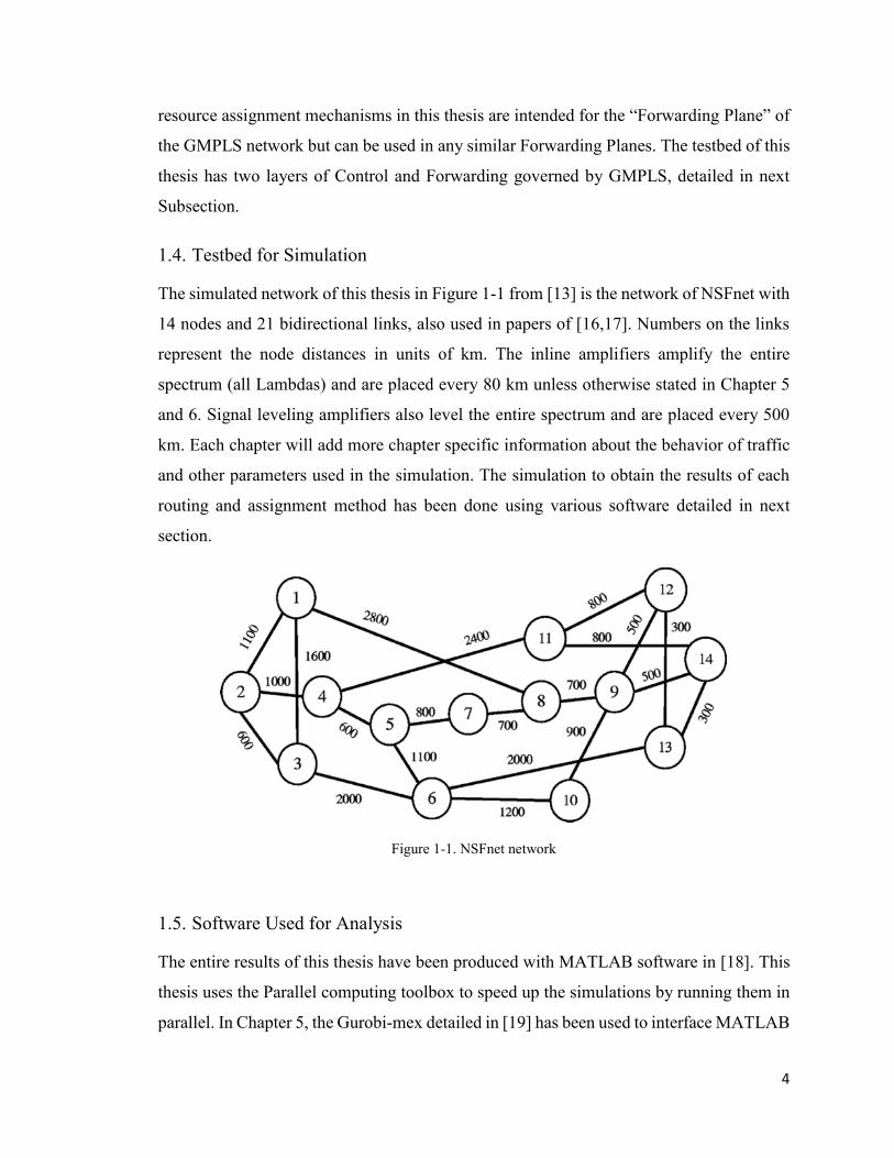
The simulated network of this thesis in Figure 1-1 from [13] is the network of NSFnet with
14 nodes and 21 bidirectional links, also used in papers of [16,17]. Numbers on the links
represent the node distances in units of km. The inline amplifiers amplify the entire
spectrum (all Lambdas) and are placed every 80 km unless otherwise stated in Chapter 5
and 6. Signal leveling amplifiers also level the entire spectrum and are placed every 500
km. Each chapter will add more chapter specific information about the behavior of traffic
and other parameters used in the simulation. The simulation to obtain the results of each
routing and assignment method has been done using various software detailed in next
section.
Figure 1-1. NSFnet network
1.5. Software Used for Analysis
The entire results of this thesis have been produced with MATLAB software in [18]. This
thesis uses the Parallel computing toolbox to speed up the simulations by running them in
parallel. In Chapter 5, the Gurobi-mex detailed in [19] has been used to interface MATLAB

5
with the Gurobi optimization solver in [20] to solve the Linear Programming problem for
routing. Chapters 5 and 6 have use the Minitab in [21] to calculate the Confidence
Intervals (CIs) for the performance metrics. The next section details the organization of
this thesis and upcoming chapters.
1.6. Organization of Thesis
This thesis has six more chapters as follows:
Chapter 2: reviews the related works in the literature and explains their link to new topics
introduced in this thesis.
Chapter 3: introduces two new stateless routing and assignment mechanism for the GMPLS
network that can increase the throughput of the control plane in serving connection requests
by up to 6-fold, published in papers of [22,23].
Chapter 4: studies the effect of adopting Green SLA (GSLA) on the behavior of key
performance metrics of the GMPLS networks. The Chapter 4 published in [24], suggest
more investment on green energy infrastructure. This chapter also defines and considers
Green Service Level Agreement (GSLA detailed later) for routing mechanisms by
proposing a mathematical model for route greenness and proposing two algorithms for the
adoption of GSLA. The results of this paper show that adoption of the GSLA by routing
mechanisms decrease the resource efficiency in return for a smaller reduction in emission
as compared to the other Green routing mechanisms. This Journal paper also emphasizes
the importance of developing better “green-aware” mechanisms. Chapter 4 is provided as
it published, due to license limitations.
Chapter 5: is the extended version of the paper published in [15] which introduces a multi-
SLA aware routing mechanism that considers multiple constraints in forwarding traffic and
uses a set of practical energy information. The routing method introduced by this chapter
is more SLA compliant and emission efficient compared to other methods reviewed in the
chapter. The method introduced in this chapter provides up to 35% % emission reduction
while maintaining 100 % SLA satisfaction.

6
Chapter 6: introduces a new resource assignment mechanism that improves the success rate
of the network when compared to the traditional resource assignment of First Fit with the
continuity constraint in resource assignment. The assignment method of this chapter
provides to 36% less energy when compared to the usage of First Fit without the continuity
constraint.
Chapter 7: draws the conclusion and states the future work.
7
Chapter 2 A REVIEW OF RELATED WORK IN THE FIELD OF
GREEN ROUTING AND RESOURCE ASSIGNMENT
MECHANISMS
This chapter provides the reader with some insight into the technical background on the
foundation work of this thesis. This chapter is segmented as follows: Section 2.1 reviews
the Service Level Agreements used in this thesis. Section 2.2 reviews the energy and
emission efficient routing mechanisms that form the foundation of the new methods
introduced in this thesis. Introduction to Emission Topology Database is also visited in
Section 2.2. Section 2.3 reviews the concept of Emission Topology Change and explains a
routing method that initiates the reprovisoning of established connections due to a change
in emission topology database. Section 2.4 reviews the resource allocation mechanism used
in the reconstructed or new methods of this thesis. Section 2.5 reviews the power state of
elements of the forwarding layer, followed by Section 2.6 that reviews a few Integer Linear
Programming methods intended for routing and assignment in optical networks.
2.1. Service Level Agreements used in Green Networks
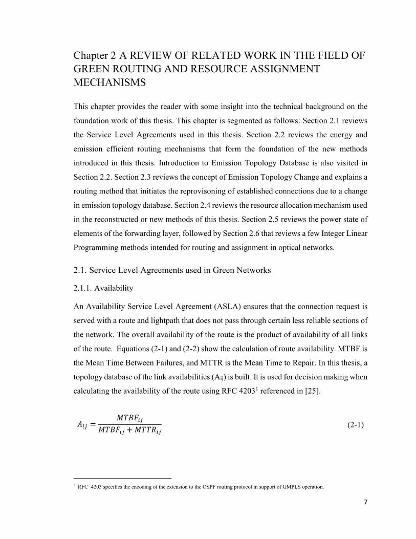
2.1.1. Availability
An Availability Service Level Agreement (ASLA) ensures that the connection request is
served with a route and lightpath that does not pass through certain less reliable sections of
the network. The overall availability of the route is the product of availability of all links
of the route. Equations (2-1) and (2-2) show the calculation of route availability. MTBF is
the Mean Time Between Failures, and MTTR is the Mean Time to Repair. In this thesis, a
topology database of the link availabilities (Aij) is built. It is used for decision making when
calculating the availability of the route using RFC 42031 referenced in [25].
𝐴𝑖𝑗 =𝑀𝑇𝐵𝐹𝑖𝑗
𝑀𝑇𝐵𝐹𝑖𝑗 + 𝑀𝑇𝑇𝑅𝑖𝑗 (2-1)
1 RFC 4203 specifies the encoding of the extension to the OSPF routing protocol in support of GMPLS operation.

8
𝐴𝑅 = ∏ 𝐴𝑖𝑗(𝑖,𝑗)∈𝑅
(2-2)
The papers in [26-28] have proposed, and used, a topology database for maximum route
availabilities (AR) using the same extended link availability attributes. In this thesis,
although the requested Availability of the connection requests is considered when fining a
route (also in [29]) with all proposed routing methods of this thesis, the route availability
topology database is not populated. The first reason is that more than one route is found in
the initial route calculation of the routing methods of Chapters 3 and 4, similar to the
method in [13,30]. Therefore, more than one route availability is needed. The second
reason is, there may be no resources left (Lambda) to forward a new lightpath through the
route whose availability is given by the route availability table, and therefore a new route
and a route availability calculation may be needed.
A route R, with lower availability may be assigned to a connection by paying penalties to
the requester of a connection, or by an accompanying backup route (To improve the overall
Availability) to be used in the event of failure of the primary path.
2.1.2. Delay
A Delay Service Level Agreement (DSLA) specifies the total end-to-end delay for the
lightpath or route R. The end-to-end delay of the route serving a connection request must
be less than the value specified in DSLA. The end-to-end delay of the lightpath from source
node S to destination node D comes in Equation (2-3):
𝑇𝑅 = ∑ 𝑇𝑖𝑗(𝑖,𝑗)∈𝑅
+ ∑ 𝛿𝑗𝑗∈𝑅 ,𝑗≠𝑆 𝑗≠𝐷
(2-3)
In which Tij is the time delay for the light to traverse each link (i,j) of the route R, and 𝛿𝑗
is the amount of delay in Lambda or resource conversion. DSLA in this thesis is concerned
with establishing the lightpath in core nodes and delays in access and aggregate nodes are
not considered. The DSLA as a constraint for finding a route is studied in Chapter 5.

9
2.1.3. Greenness
A Green Service Level Agreement (GSLA) as defined in [31,32] specifies the minimum
percentage of green energy to be used while serving a customer. The reason for the
introduction of this SLA as mentioned in Section 1.3, is to reduce the emission and promote
the usage of green energy. With considering GSLA, the amount of reduction in emission
can be quantified and measured for compliance. It is possible that companies that provide
service to government organizations may be asked to use a minimum percentage of green
energy for their continued contract with governments. On the other hand, government
organizations and the bigger segment of the private sector may refuse to do business (due
to government penalties, higher taxes, etc.) with organizations that do not conform with
green policies of the Provincial or Federal government. However, as with other SLAs,
GSLA also faces an interesting challenge. Per framework introduced in [33], GSLA also
needs a trusted third party Moderator for monitoring the compliance and logging the
violations. It is also very cumbersome to monitor the GSLA violation from the technical
point of view. On the other hand, the type and value of the penalties must be negotiated for
a different amount of violations.
Chapter 4 defines the ratio of a total number of “Green Powered” inline amplifiers over
the total number of amplifiers of a lightpath, as a basic definition for GSLA in GMPLS
networks.
In Chapter 5 a new definition for greenness is considered as explained in Chapter 5.
2.2. Routing Mechanisms
2.2.1. Emission as a Route Cost and Traffic Engineering Extensions for OSPF
Authors of the paper in [34] have introduced a new opaque LSA to propagate the link
energy type (e.g. coal, wind, etc.) and build an emission topology database table knowing
the link energy usage. This thesis uses the same LSA to build the same emission topology
database conceptually shown in Equation (2-4) for a network with n nodes.

10
𝑀𝑛×𝑛 = [
∞ ⋯ 𝑚1𝑛
⋮ ⋱ ⋮𝑚𝑛1 ⋯ ∞
] (2-4)
In Equation (2-4) mij is the emission of the link connecting node i to node j. The member
of the main diagonal of the Mnxn matrix, as well as the value for non-existent links(when
there is no link between node i and j), are considered infinity. The same emission topology
database is used in Chapters 3 and 4. This topology database is similar to other Traffic
Engineering (TE) topology databases created in the control plane and is used for finding a
route, or calculating the emission of a network. Chapters 5 and 6 use a different type of
LSA as detailed later in Chapter 5.
The authors in [11,35] have introduced a routing mechanism that finds the least or shortest
emission first route for connecting a source node to a destination node. The method in these
papers considers emission topology database in Equation (2-4) for finding the lowest
emission route as also detailed in [34]. The shortest emission method is called Energy
Efficient method (EE) in corresponding papers. EE is not an SLA-aware mechanism and
uses more resources compared to traditional shortest path method (per corresponding
papers), to serve an equal number of connection requests, as elaborated in [11,13,35].
However, it performs very well regarding emission reduction when compared to the
shortest path method, again, based on corresponding papers. The EE has been reconstructed
in the analysis sections of upcoming chapters for comparison against other proposed
methods. The next section introduces a green routing mechanism that considers the
resource utilization factor in serving a connection request, by using a hybrid cost.
2.2.2. Hybrid Cost of a Route
The concept of Hybrid green cost is introduced in the paper of [13]. The hybrid green cost
which can be considered as a TE cost, pursues two goals: Minimizing the length of the
route, and reducing the emission of the route, while being ASLA compliant. The routing
mechanism that uses this hybrid cost as defined in the paper of [13] is called the Emission
Aware and SLA Based routing mechanism or EASB. EASB first calculates the k most-
available routes from a source node to a destination node using Equation (2-5). Equation

11
(2-5) gives the logarithmic value of the Availability of route R, as the cost of the route CR,
given the link availability of Aij as explained in Section 2.1.1.
𝐶𝑅 = ∑ − ln(𝐴𝑖𝑗)
(𝑖,𝑗)∈𝑅
(2-5)
EASB then calculates the Emission Factor of each route (EFR) for each of the k routes
using Equations (2-6). EASB then calculates the hybrid cost of each of the k routes using
Equation (2-7). Finally, EASB serves the connection request with a route that has the
minimum of the hybrid cost and complies with the ASLA of the connection request.
𝐸𝐹𝑅 = ∑ 𝑙𝑖𝑛𝑘_𝐶𝑜2𝑖,𝑗
(𝑖,𝑗)∈𝑅
(2-6)
𝐶𝑜𝑠𝑡𝑃 = 𝛼×𝜆𝑅 + (1 − 𝛼)×𝐸𝐹𝑅 (2-7)
In Equation (2-7), 𝜆𝑅 is the length of the route in units of hops and 𝛼 = 0.35 is a balancing
factor as explained in the paper of EASB in [13] that provides the lowest normalized hybrid
cost for the combination of emission factor (EFR) and 𝜆𝑅 as we can see in Figure 2-1 for
the testbed network of this thesis.
Figure 2-1. Hybrid cost vs value of 𝛼

12
EASB is not aware of GSLA or DSLA however it has an acceptable resource utilization
when compared to EE and traditional non-green routing method, detailed in the
corresponding paper for EASB. Figure 2-2, directly from the corresponding paper details
the operation of EASB.
Get next connection
request
Get source, destination, and the requested availability of the
connection
Calculate k most available paths between source and destination
using Yen’s k-shortest path algorithm
Calculate the Co2 emission factor of
all k possible paths based on Co2 emission factor table using (2-6)
Path available?Block the
connection
Establish the
connection
NO YES
Calculate the hybrid cost for each path based on the path length
and the Co2 emission factor using (2-7)
Update network graph, network resources, and Co2 factor table
Find the path with the minimum hybrid cost which meets
requested path availability constraint among k calculated paths
Modify links cost based on the availability of links using (2-5)
Figure 2-2. Routing with hybrid cost

13
EASB as an intuitive method with acceptable resource utilization as per [13,23] has also
been added to the simulation and analysis sections of upcoming Chapters 3, 4 and 5. New
routing mechanisms introduced in this thesis will be compared against EASB for resource
utilization and other performance metrics detailed in corresponding chapters. Chapter 3 of
the thesis builds a routing table for serving the connections using EASB method and shows
that by using a routing table the throughput of the control plane (ability to serve connection
requests) can be increased by 6-fold. EASB uses the same emission topology database of
EE. Chapter 4 adds the GSLA awareness to EASB and analyse the effect of adopting this
SLA on the behaviour of key performance metrics. Next section is reviewing the concept
of emission topology change and modified EASB to reprovision the established
connections.
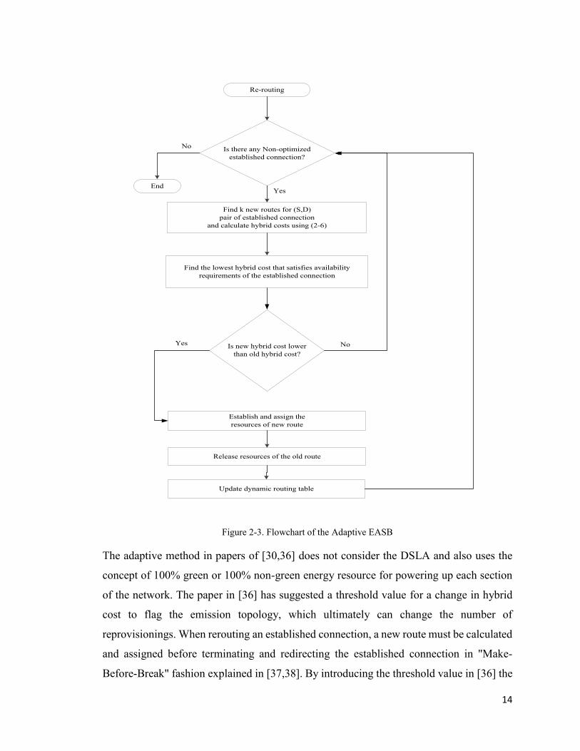
2.3. Emission Topology Change and Adaptive Re provisioning
The papers in [30,36] have explained the situation in which the source of energy powering
up each section of the network is changed. The emission of energy powering up each
section of the network can change as green energies such as solar and the wind are available
on limited bases and can change in hours. When the type of energy (or greenness of the
energy) powering up each section of the network is changed, the emission topology
database of the Equation (2-4) has to be updated with new link emission before serving the
new connection requests. After updating or repopulating the emission topology database,
the new connection requests can be served with new emission information. Similar to other
types of topology change (e.g. link failure), a reprovisioning mechanism is triggered in the
papers of [30,36] to re-optimize the currently established lightpaths to reduce the emission.
The reoptimization is done because the established lightpaths might not be in an optimized
emission state as the emission of a route can change when an emission topology change
happens. The detail of the reprovisioning operation is shown in the flowchart of Figure 2-3.
14
Re-routing
Is there any Non-optimized
established connection?
Find k new routes for (S,D)
pair of established connection
and calculate hybrid costs using (2-6)
Update dynamic routing table
Find the lowest hybrid cost that satisfies availability
requirements of the established connection
Establish and assign the
resources of new route
Release resources of the old route
Is new hybrid cost lower
than old hybrid cost?
End
NoYes
No
Yes
Figure 2-3. Flowchart of the Adaptive EASB
The adaptive method in papers of [30,36] does not consider the DSLA and also uses the
concept of 100% green or 100% non-green energy resource for powering up each section
of the network. The paper in [36] has suggested a threshold value for a change in hybrid
cost to flag the emission topology, which ultimately can change the number of
reprovisionings. When rerouting an established connection, a new route must be calculated
and assigned before terminating and redirecting the established connection in "Make-
Before-Break" fashion explained in [37,38]. By introducing the threshold value in [36] the

15
established route is not altered, and the assignment phase of Make-Before-Brake is
avoided, when there is not a significant (more than the threshold) change in the hybrid cost
of the route. Effect of re provisioning with A-EASB on Green SLA compliance has been
studied in Chapter 4. The next section reviews the Lambda assignment methods used in
this thesis.
2.4. Resource Assignment Methods
This section lists a few important resource assignment methods from the report in [39] and
the paper in [40]. First Fit (FF) and FF with the continuity constraint in assignment as
detailed below are used in upcoming chapters of this thesis. More detail on the setup and
pairing with routing method is given in each subsequent chapter.
2.4.1. Random
This method assigns a random Lambda number to each hop of a lightpath passing through
the optical links. This method is a very easy and intuitive way of assigning the Lambda
(Resource) however since it does not consider the Continuity Constraint (explained later)
it may need more “Lambda Conversion” which adds to the energy consumption, and
increases the end-to-end delay of the lightpath.
2.4.2. First Fit
The First Fit (FF) method assigns the first available Lambda number to the lightpath
passing through each optical link. For simplicity and to be consistent with other related
work FF method has been used in the proposed routing methods of this thesis. Chapters 5
and 6 use FF with continuity constraint. Furthermore, Chapter 6 benchmarks the
performance of a new assignment mechanism against FF and FF with the continuity
constraint which is discussed next.
2.4.3. Continuity Constraint
The continuity constraint, continuous, or CNT as explained in [39] is a situation in which
the same Lambda number is assigned to a lightpath for all links of the route. Considering
the continuity constraint adds to the complexity of assigning a Lambda for a lightpath,
however it has the advantage of saving energy (since no Lambda conversion is performed),
16
and decreasing the end-to-end delay of the lightpath. The percentage of energy saving and
decrease in the delay has been studied and simulated in Chapter 5 of this thesis with the
newly proposed routing mechanism of Chapter 5.
To be able to save energy, the energy state of the optical elements must be known to the
assignment method. Depending on the number and type of power states of optical elements,
different routing and assignment methods can be chosen to serve a connection request. The
next section details the power state of the elements used in the simulation and analysis
section of each chapter.
2.5. Optical Forwarding Element and Their Operational States
In this thesis, the forwarding elements of the network that have no role in directing any
lightpath may be placed in the OFF state and unlike the paper in [41-44] no sleeping mode
or state is considered. Sleeping mode reduces the life time of equipment and is
economically infeasible as discussed in [45]. In this thesis, the elements of the control plane
or the electrical control and decision-making plane are considered ON at all times as they
perform the routing and re-provisioning task for the lightpaths. When performing Make-
before-Break re-provisioning for lightpaths or Traffic Engineering tunnels of MPLS, the
control plane may wait for the period of the “wake up duration” or boot duration of a router
(when the control plane is turned ON) and then switch over to the newly provisioned route.
However, in the event of failure, the already calculated backup path must be used right
away in similar fashion to the Fast Reroute mechanism in [46] to mitigate the effect of
failures, such as SLA violation and data loss. Therefore, wake up time may cause an ASLA
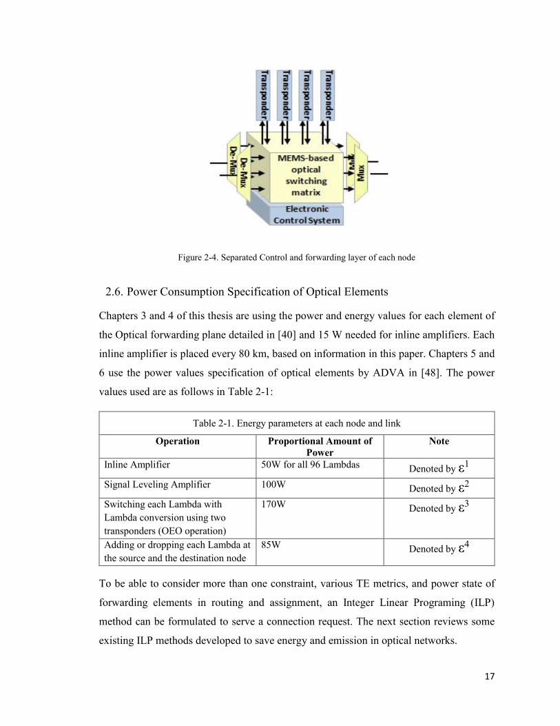
and DSLA violation and penalties to the Service Providers. Figure 2-4 from [40] shows the
separated electronic control plane of a node. In this thesis power reduction and optimization
is performed for the optical or forwarding plane only, since the increase in power
consumption of the control plane is increased by 3% only, per work in [45,47] and may be
considered constant. The specification and power rating of each forwarding element is
gathered in the upcoming section.
17
Figure 2-4. Separated Control and forwarding layer of each node
2.6. Power Consumption Specification of Optical Elements
Chapters 3 and 4 of this thesis are using the power and energy values for each element of
the Optical forwarding plane detailed in [40] and 15 W needed for inline amplifiers. Each
inline amplifier is placed every 80 km, based on information in this paper. Chapters 5 and
6 use the power values specification of optical elements by ADVA in [48]. The power
values used are as follows in Table 2-1:
Table 2-1. Energy parameters at each node and link
Operation Proportional Amount of
Power
Note
Inline Amplifier 50W for all 96 Lambdas Denoted by ε1
Signal Leveling Amplifier 100W Denoted by ε2
Switching each Lambda with
Lambda conversion using two
transponders (OEO operation)
170W Denoted by ε3
Adding or dropping each Lambda at
the source and the destination node
85W Denoted by ε4
To be able to consider more than one constraint, various TE metrics, and power state of
forwarding elements in routing and assignment, an Integer Linear Programing (ILP)
method can be formulated to serve a connection request. The next section reviews some
existing ILP methods developed to save energy and emission in optical networks.
18
2.7. Integer and Mixed Integer Programming Formulation of Optical and
Optical/Electrical Networks
The entire section here details the papers with Integer Linear Programing (ILP) or Mixed
Integer Programming (MIP) for optimizing power and emission in optical networks. These
methods are the “Power Models” that are formulated depending on the type of the network
and type of the optical equipment used in the network. The work in [14,42,49] have
proposed the three State of ON, OFF and SLEEP for network elements and tried to
maximise the amount to “sleeping” elements when possible. Paper in [49] attempts to
optimize the optical network so that all 1:1 protection paths are placed in sleep mode, and
it is called “Minimum Power with Devices in Sleep Mode Strategy.” The work in [14] tries
to maximize the elements that are supporting 1:1 backup protection role to maximize the
number of sleeping devices. As mentioned before, no sleeping mode or state is considered
in this thesis. The paper in [49] also attempts to minimize the power with or without sleep
mode, however, does not consider the type of energy or percentage of the greenness of
energy powering ON the networking elements. The work in [50] also explains the
complexity of the Mixed Integer Linear Programming (MILP) approach in detail. The
proposed approach in Chapter 5 tries to minimize the complexity of the ILP and keep it in
order of O2. The new routing mechanism introduced in Chapter 5 of this thesis uses a simple
yet effective ILP formulation for fast resolution time (less than a second).
Reference [51] has formulated a very detailed model for reducing the energy in optical
elements of the network which consists considering the node energies as well as link
energies. Although the model is very comprehensive, it fails to return a result after a full
day of intensive computation as stated in the paper. The result of computation in this case
means having a route that complies with all constraints, or determination of the situation
in which the model is infeasible, and quitting the computation. One attempt in this thesis
and Chapter 5 to simplify the ILP method is to eliminate the constraint number 6 of the “E-
TESP” model in this paper which is a constraint about availability of the resource in the
optical links of the route to be used for serving the connection request. In this thesis, a
dynamic network is used for calculating the route in all chapters of the thesis. The dynamic
network means that when the last resource of a link is assigned, the link is taken out from
the network topology and is not used for routing the later connection requests.

19
The work in [45] has proposed a very detailed model for energy when combining optical
and non-optical networking elements for assigning the resources and has come up with
three comprehensive formulations for energy consumption and emission. The paper in [45]
work has proposed a formulation for maximizing the energy difference between non-green
and green energy to maximize the use of green energy. In another approach, it also has
proposed a formulation to minimized the total energy used in the network, minimizing the
cost of Routing and Wavelength Assignment (RWA) formulation and minimizing total
GHG emitted. The paper in [45] also suggests some key information about the amount of
energy used for transporting a single Lambda for transparently passing, converting to other
Lambda number, and when performing optical to electrical conversion (OEO). The
formulation of ILP method of Chapter 5 is inspired by the detailed information about
Lambda conversion mechanism proposed in the paper of [45], with dropping a Lambda at
the intermediate node and adding it back to perform the Lambda conversion. Based on the
paper of [45] this thesis also assumes that the lightpath is not splitable : “the traffic is
unsplittable in the optical domain: i.e. a traffic demand is routed over a single lightpath;
(in theory, in the electronic domain a demand may be splitted into n flows, but in the optical
domain these will appear as an unsplittable optical flows)“.
The work in [52] has performed a detailed analysis on the power consumption of IP over
WDM network and has formulated an objective function to minimize the number of
required Lambdas or resources between any given nodes when the traffic pattern is known.
This work also provides some power values for elements that were used in the initial
simulations of the proposed work until the detailed specification of modern equipment
were gathered. The paper in [52] also compares the various architectures for the optical
network including the forwarding method used in Chapter 6.
The paper in [53] proposes energy aware resource allocation for a scheduled demand.
Although this paper introduces a simple and effective model for reducing the energy, it
does not consider the various SLAs such as Availability and Delay in finding a route before
assigning the resources. Without considering the availability SLA, it is not possible to
prioritise the requests that have higher importance and priority with the higher Availability
needed. When the ASLA of the request is recognized, the lightpath of the connection can

20
be routed though links that have higher Availability and resource of links with a higher
Availability can be used with higher priority connection requests.
Reference [54] defines the QoS as the maximum capacity of the link and no other SLAs or
other QoS parameters are considered as a constraint in finding a route. Later in the paper
an ILP method only uses the flow conservation constraint in finding a route. The proposed
method of Chapter 5 considers ASLA, DSLA Flow conservation constraints, and subtour
elimination constraints as constraints to be met when finding a route.
None of the papers in this section considers the energy greenness and formulating a model
for reducing the emission as opposed to the energy of the network. The method of Chapter
5 ensures that links with higher greenness are used first before using the less green links of
the network.
21
Chapter 3 DYNAMIC STATELESS SLA AWARE ROUTING
MECHANISM
This chapter details the proposed routing methods of Table Driven EASB (T-EASB) and
Forward Looking EASB (FL-EASB), published in [22,23]. These papers elaborate two
Table Driven routing and wavelength assignment mechanisms which are intended to
increase the throughput of the control plane of the GMPLS networks. T-EASB and FL-
EASB methods are based on Table Driven Design of Chapter 2 of the book in [55] and the
Hybrid Emission Aware and SLA Based (EASB) routing mechanism detailed in Section
2.2.2. The application of the table in this chapter is to transform the given information:
source node and a destination node, to a set of routes between the source node and the
destination node. These routing methods intend to reduce the time needed for finding a
route for connection request before being assigned.
3.1. Introduction
Both Table Driven Emission Aware and SLA Based (T-EASB), and Forward Looking
Emission Aware and SLA Based (FL-EASB) perform a “Route Lookup” from a routing
table which is populated beforehand as opposed to calculating a route for each connection
request. Since a route is looked up for a connection and checked for availability of the
resources to establish the lightpath, these routing methods are stateless routing
mechanisms. Stateless in the sense that the routing mechanism does not need to be aware
of the availability of the resources for the route when serving the connection request. The
assignment method (which is the First Fit without the continuity constraint as explained in
[39] and 2.4.2) tries to assign the resources of the given route. If the assignment is
successful, the connection is established. If the assignment is not successful, the route that
was looked up is marked as unavailable, and next best route to destination is considered
for assignment. This process continues up to k-times (as k routes are stored for each source-
destination pair) to find and assign a route for the connection request. Although this
operation may seem lengthy, the results of analysis in the paper of T-EASB shows that in
the worst-case scenario (assigning the resources for the last route in the table) the
throughput of the control plane is increased by 6-fold when compared to the EASB. FL-

22
EASB in [22] was introduced to deal with a situation with T-EASB in which some requests
may be blocked as the routing table is being populated and is not ready. FL-EASB
populates the routing table, beforehand, forecasting the energy and emission status of the
links for the upcoming 3 to 6 hours. In this thesis 3 to 6 hour is the time for emission
topology change and updating the energy state of each element in the simulation part of
the analysis. FL-EASB can consider the upcoming scheduled maintenance windows for
each link (if needed) to avoid using a link in populating the routing table which is used 3
to 6 hours later.
3.2. Stateless Routing and Assignment Operation
Each cell of the routing table R denoted by rsd is populated first with a stack of k-most-
available routes between each source-destination (sd) pair of nodes. Since lightpaths in
GMPLS networks are established in a bidirectional fashion based on RFC in [56], the return
path is also needed for a connection request which the same “reversed” route in this thesis.
Therefore, there is no need to calculate the return route for destination-source pairs. This
means that only half of the routing table must be populated and the return paths are the
transpose of “reversed routes” in all stacks as can be seen in Figure 3-1. In other words,
(n)*(n-1)/2 k-most-available route operations must be performed. While populating each
rsd, the hybrid cost introduced in Section 2.2.2 using Equation (2-7), is also calculated and
saved in a separate table of Hcost. Each route in the stack of rsd is marked as “accessible”
denoted by rsd_access, which means that route is available to be assigned and used. After this
step, the control plane is ready to serve the connection requests.
Figure 3-1. n by n routing table R

23
The R table is repopulated when emission topology change happens as mentioned in
Section 2.3, since the emission value and the Hcostsd for affected routes by emission
topology change are different. T-EASB is highly efficient if the total number of connection
requests per each topology change interval (e.g. 3 hours) is more than a total number of
calculated routes of the R table. When a connection request is received, the routes from rsd
cell of the R table, and the list of Hcost are fetched. After this step, the control plane chooses
the route with minimum Hcostsd that meets the ASLA of the connection request. If there is
such a route (it is accessible), the control plane tries to assign the resource (Lambdas) of
the chosen route using the FF method. If the assignment is successful, the request is served
and the dynamic resource table that keeps track of available to assign Lambdas of each link
is updated. If the assignment is not successful (because no Lambdas are available to assign
in a link of the route), the route is marked as “inaccessible” in the stack, and the next route
with the lowest hybrid cost that meets the ASLA is chosen, and the process of resource
assignment is repeated. If no route is “accessible”, the connection request is blocked. When
a lightpath is terminated, the Lambdas of the route are released, and the route is flagged as
accessible in the stack. Table 3-1 shows the pseudocode of process of populating the R
table.
Table 3-1: Creation and Population of table R
FOR (s=1: n)
FOR ( d=s+1: n )
rsd = k_shortestpath(s,d);
FOR (i=1:k)
Hcostsdi = Calculate the hybrid cost for rsdi using (2-7); rsdi_access=True;
rdsi = Reversed (rsdi); Hcostdsi = Hcostsdi ; rdsi_access=true;
END
END
END
Figure 3-2 shows how a connection request is handled. FL-EASB is the same as T-EASB
except for the fact that it populates the R table 3 to 6 hours ahead of the time using the
predicted information about the sources of energy for each link.

24
Figure 3-2. Handling a connection request
With 100% accuracy in predicting energy source of each link T-EASB and FL-EASB
become the same. The prediction for the source or type of energy producing the electricity
is done by power generation companies as they need to manage the demand for the
upcoming hours. Power generation companies monitor the reports from weather
forecasting agencies about the availability of sun and the wind to predict the production of
green energy for the upcoming hours. When not enough green energy is “forecasted” to be
available, power generation companies increase the usage of non-green energies to cope
with the demand for electricity. On the other hand, when green energies are available the
power companies can reduce the usage of non-green energies to reduce the emissions. A
wrong prediction in this chapter means observing another unexpected outcome about the
source of energy and ultimately different outcome for the greenness of energy of a link.
Handling request
Fetch the rsd stack of routes for
source-destination pair of
connection request
Find the route in R_Hcost that has
lowest hybrid cost, is accessible, and
meets the SLA requirements of the
connection request
Can route of tunnel be
signaled?
Reserve the
resources(lambdas) of
the route
Update the dynamic
resource table
Wait for next
request
Mark the route as
“inaccessible” in the
stack of routes
YES
Is there any route?
NOBlock the
request
YES
NO

25
For example, having a cloudy day despite the forecasts for having a sunny day and being
forced to compensate the missing portion of the energy needed in a section of the network
that otherwise could be generated by solar panels and other solar technologies on a sunny
day.
3.3. Analysis
3.3.1. The Simulation Network
The simulation network topology is the NSFnet network presented in Figure 1-1 and
repeated here as Figure 3-3. Each inline amplifier is placed at every 80 km of optical links.
Any type of energy sources can power nodes and links in the network, and the information
about the type of energy of each link is disseminated through the network using the
extended Link State Advertisements for energy as proposed in [34,35]. To deal with
dynamic routing requests, it is assumed the routing and signaling information is propagated
using the Resource Reservation Protocol or RSVP in [57] The duration of the connections
follows an exponential distribution with a mean of 6 hours. The Co2 emission for each
source of energy powering nodes and optical links of the network has been adopted from
the greenhouse gas emissions values provided in work [10]. Availability SLA (ASLA)
requested by connection requests ranges between 0.999 to 0.99999. The availability of the
links is assigned a random number between 0.9999 to 1 and does not change for the period
of simulated time, 30 days.
Figure 3-3. NSFnet network

26
3.3.2. Performance Metrics Used in This Work
EASB, T-EASB, FL-EASB, EE and a modified non-green routing method called k SLA
Based (KSB) in [58] are benchmarked in this chapter. KSB first computes the k-most-
available routes from a source node to a destination node and then serves the connection
request with the shortest (units of hop) computed route that meets the ASLA of the
connection request. The accuracy of the predictions for the energy source is kept at 95%
when using FL-EASB routing mechanism.
ASLS
ASLS is the Satisfaction rate of the ASLA. This is a ratio of the number of connections
that were served with a route that met their ASLA to the total number of the servered
connections. FL-EASB, T-EASB, KSB and EASB that consider ASLA in finding a route
for a connection request, result in 100% ASLA satisfaction.
Success Rate
The success rate is the ratio of the number of served connection requests over a total
number of connection requests.
Lambda per Connection
This is the average length of the lightpath of the served connections in units of hops. A
lower number is preferred for this metric. The lower the number, the more resource
efficient is the routing mechanism.
Emission per Lambda
This metric is the amount of emission emitted to the atmosphere to establish a unit resource
Lambda. A lower number is preferred for this metric. This metric shows the emission
reduction capability of a routing mechanism. The value of the emission per Lambda will
be lower for the routing mechanisms that have a higher success rate as the total emission
is divided by more number of resources in operation, resulting a lower average emission.
Because of this reason emission reduction must be evaluated and analysed among routing
methods that have about the same success rate.
27
3.4. Results
3.4.1. Performance Benchmark
As we can see in Figure 3-4, overlapping EASB and T-EASB reduce the emission of the
network by 21% compared to the non-green method of KSB. FL-EASB performs
marginally the same with prediction up to an average of 95% accurate. The difference in
emission reduction is only 2 g Co2 per Lambda. The pure green method of EE, not
surprisingly, provides the lowest emission per unit resource Lambda. The result of analysis
for average connection length in Figure 3-5 shows that EASB, T-EASB, and FL-EASB
have almost identical resource efficiency and consume only about 10% more resources
compared to the non-green method of KSB. The reason is, the EASB family of routes find
a route with minimum hybrid cost that satisfies the ASLA of the connection request. The
route with the lowest hybrid cost that satisfies the ASLA may be longer trying to bypass
the non-green sections of the network, therefore, is not the shortest route that complies with
the ASLA of the connection request. As we can see in Figure 3-5, EE increase the average
route length by about 57% when compared to KSB. This is because EE tries to find the
greenest route and bypass the most of non-green sections of the network and uses longer
routes. For the percentage of ASLS shown in Figure 3-6 we can see that all routing
mechanism that consider ASLA constraint in finding a route for the connection request,
give 100% satisfaction for the connections they serve. Without considering the ASLA for
finding a route, ASLS can drop by more than 20% with EE. This may or may not be
acceptable since the resources for the lightpaths have been assigned, and the lightpath has
been established, since as we will see in Figure 3-7, EE has 100% success rate, and no
connection request has been blocked. In Figure 3-7 we can see that EASB, T-EASB and
FL-EASB perform the same regarding the number of the connection they serve. This is
very important as T-EASB and FL-EASB did the routing by lookup and not the actual “per
connection requests calculation.” As we can see almost 10% of connection request were
blocked since there was no route to satisfy their ASLA.
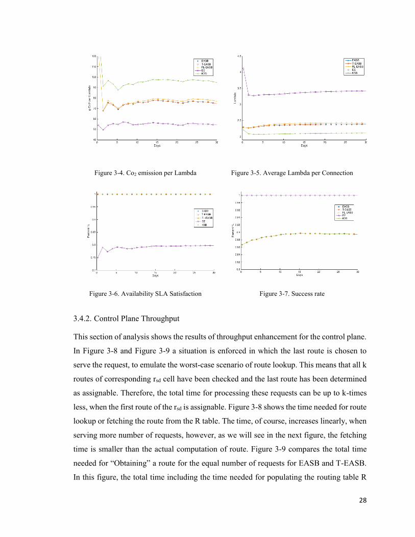
28
Figure 3-4. Co2 emission per Lambda Figure 3-5. Average Lambda per Connection
Figure 3-6. Availability SLA Satisfaction Figure 3-7. Success rate
3.4.2. Control Plane Throughput
This section of analysis shows the results of throughput enhancement for the control plane.
In Figure 3-8 and Figure 3-9 a situation is enforced in which the last route is chosen to
serve the request, to emulate the worst-case scenario of route lookup. This means that all k
routes of corresponding rsd cell have been checked and the last route has been determined
as assignable. Therefore, the total time for processing these requests can be up to k-times
less, when the first route of the rsd is assignable. Figure 3-8 shows the time needed for route
lookup or fetching the route from the R table. The time, of course, increases linearly, when
serving more number of requests, however, as we will see in the next figure, the fetching
time is smaller than the actual computation of route. Figure 3-9 compares the total time
needed for “Obtaining” a route for the equal number of requests for EASB and T-EASB.
In this figure, the total time including the time needed for populating the routing table R
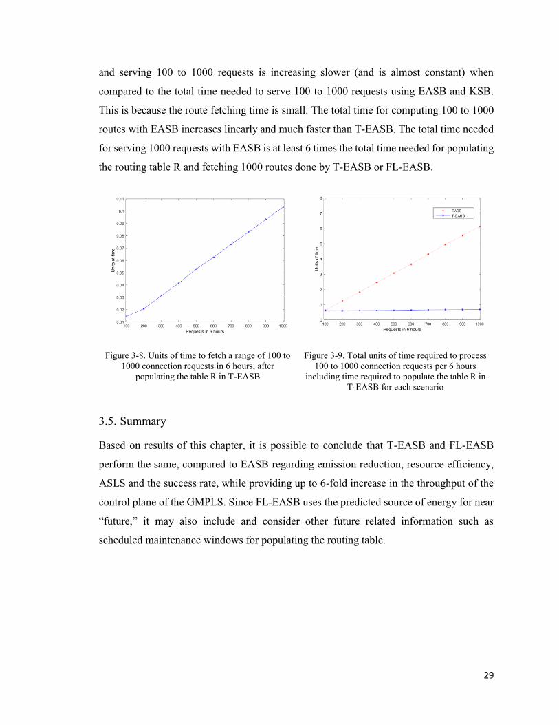
29
and serving 100 to 1000 requests is increasing slower (and is almost constant) when
compared to the total time needed to serve 100 to 1000 requests using EASB and KSB.
This is because the route fetching time is small. The total time for computing 100 to 1000
routes with EASB increases linearly and much faster than T-EASB. The total time needed
for serving 1000 requests with EASB is at least 6 times the total time needed for populating
the routing table R and fetching 1000 routes done by T-EASB or FL-EASB.
Figure 3-8. Units of time to fetch a range of 100 to
1000 connection requests in 6 hours, after
populating the table R in T-EASB
Figure 3-9. Total units of time required to process
100 to 1000 connection requests per 6 hours
including time required to populate the table R in
T-EASB for each scenario
3.5. Summary
Based on results of this chapter, it is possible to conclude that T-EASB and FL-EASB
perform the same, compared to EASB regarding emission reduction, resource efficiency,
ASLS and the success rate, while providing up to 6-fold increase in the throughput of the
control plane of the GMPLS. Since FL-EASB uses the predicted source of energy for near
“future,” it may also include and consider other future related information such as
scheduled maintenance windows for populating the routing table.

30
Chapter 4 GREEN SLA AUGMENTED EMISSION AWARE
AND SLA-BASED ROUTING MECHANISM
This chapter consists of the journal paper published in [24]. Due to license restrictions for
reusing the paper without modifications, the content of this chapter comes as published.
The numbering style for figures, tables, equations and references has been updated to match
the style of the thesis. The term “this paper” has changed to “this chapter” and text has
been augmented with clarifying statements provided by the committee; however, figures,
analysis, and other results are intact. This chapter analyses the effect of adopting Green
Service Level Agreement (GSLA) on the value of the key performance metrics of the
WDM networks, as briefly mentioned in Section 2.1.3. As we will see in this chapter, 20%
increase in the chance of powering up links of the network by green energy leads to up to
90% success rate for serving connection requests that may ask for up to 80% greenness of
energy powering up the route (GSLA up to 80%). The chapter is sectioned as follows:
introduction section gives the background on the issue also explained in Chapter 1. Section
4.2 adds the chapter specific related work. The introduction to the method of adding the
Green SLA awareness comes in Section 4.3 followed by analysis section 4.4 that introduces
the setup for testing the GSLA aware mechanisms. At the end, the A-EASB introduced in
Section 2.3 is also added to analysis for testing the effect of reprovisioning on GSLA
Satisfaction. The chapter is concluded with a summary and future work. This chapter is the
only chapter that considers the GSLA. Adopting GSLA increases the resource utilization
without a justifiable amount of reduction in emission. As concluded in this chapter it is
important to invest in greener infrastructure and green routing mechanisms.
4.1. Introduction
The effect of Greenhouse Gases (GHGs) such as Co2 on global warming and formation of
the acidic rain has been at the center of attention for two decades now. According to the
study in [1] the energy needed to operate the datacenters of world’s largest network, the
Internet, is more than 2 % of the global energy produced. This numbers excludes the
energy needed to power up all the underlying optical networks and networking equipment.
This means at least 2 % of the global GHG emission is due to electricity generation needed

31
to power ON networks, if no green source of energy is used. Various methods in different
industries have been proposed to reduce the amount of energy emissions and to have
greener operations. Among other industries, IT and communication industry has also
proposed many ideas to reduce the amount of GHGs to develop greener methods and
protocols. A few of the most important and recent agreements among the industrial
countries such as the U.S. and China to reduce the amount of emissions (GHGs) is detailed
in [4,6]. The agreement between the U.S. and China in [4] sets goals on GHG emission
reduction in these two counties. The set goals will push governments to mandate industries
to adhere to some guidelines in their operation to reduce the amount of GHGs. There are
two general methods to reduce the amount of GHGs: one is to use more energy efficient
devices and equipment, and the other (not surprisingly) is to use green sources of energy.
The second method has more importance, as lowering the energy used in operation,
beyond some point, will reduce the amount of operation. Therefore, we need more green
energy and better methods to be able to use the green energy. There are two main methods
to regulate the reduction of emission adopted by some countries that are financial
incentives for the reduction of emission by an organization that participates in the emission
reduction program. The first method is Caps Trading discussed in [7] and the second is
Carbon Tax presented in [9]. The first method is the fixed cap for the GHG emissions of
an organization, meaning that an organization which needs to emit more GHG must
purchase the right to produce and emit more GHGs from another organization that will
produce less GHGs emissions. By employing this method, greener organizations can have
more income by selling a part of their cap. The second method is to set higher taxes on
carbon based sources of energy. With this approach, greener organizations pay less tax on
energy produced by using green sources of energy. In this chapter, organizations are
customers of Internet and Infrastructure Providers (Service Providers) who want to
outsource the communication infrastructure and possibly require a dedicated resource
from Service Providers based on information in [38]. These organizations require a certain
percentage of greenness for routes connecting different sections of the organization, to
reduce the amount of emission. This means customers will set Green Service Level
Agreements (GSLA) value on their requests to Service Provider to request a greener
resource up to a percentage indicated in a GSLA. One challenge in using the green energy

32
in IT industry and networking is to know which segments of a network are powered ON
by green sources of energy. The other challenge is how to use information about green
sources of energy powering up each section of a network, to steer the data flows from a
given source to any destination using green sections of the network. By doing so, non-
green sections of a network stay in hibernation or power OFF state. These challenges have
been addressed by introducing green and hybrid routing mechanisms in [13] and [34,35]
at the cost of having higher resource utilization compared to non-green methods
(explained in more details in next sections). To provide a customer with a route that meets
the requirements of the GSLA, Service Providers may choose to use the traditional non-
green routing mechanisms to compute a set of routes and then select a route that meets the
GSLA set by the customer, hoping to avoid the higher resource utilization (higher average
length of routes). However, as illustrated in this work, the usage of non-green mechanisms
may increase the resource utilization and also result in an unacceptable amount of
reduction in emission. Increased resource utilization level may not be troublesome when
traffic is light in the network, but it decreases the success rate of the network as we will
see in next sections. This chapter is organized as follows: Section 2 details the related
work in the field of green networking; Section 3 introduces the GSLA for green optical
networks and discusses a model used in this work to increase the chance of having green
sources of energy in a “Greener Network”. Section 3 also details the effect of re-
provisioning on GSLA satisfaction. Section 4 defines the variables, simulation setup, and
important metrics. Section 5 discusses the obtained results followed by Section 6 that
draws the conclusion and states the future work.
4.2. Related Work
This section briefly introduces some related work which forms the foundation of this paper.
These concepts have either been reconstructed or directly used in conjunction with analysis
for this chapter. The Emission Aware SLA Based routing mechanism (EASB) introduced
in [13] uses a hybrid metric in finding the best route for connection requests. This method
reduces the amount of emission while maintaining an acceptable amount of resource
utilization. Resource utilization in this work and in [35], is a measure of how lengthy
(average in hops) are the routes in a Service Provider network. A lower average result in

33
better or less resource utilization. This method has been reconstructed in the simulation
part of this chapter for comparison. The papers discussed in [34,35], have proposed a new
type of Opaque Link State Advertisement (LSA), originally defined in [59], to disseminate
the information about the type of energy (given by smart grid) powering up each link across
a link state area. The new LSAs are then used with a routing mechanism, which finds the
most Energy Efficient (EE) route between a given source-destination pair of nodes, (S, D).
The LSAs proposed by these papers have been used in this work to form a database of
energy types for links of the simulated network. Energy topology databases based
information from the smart grid, are the decision support table for routing and energy
management in this chapter, and are gathered in a similar manner presented in [60]. This
information is used by Service Providers to determine the greenest route among all
calculated routes when no green routing mechanism is used. The reconstructed routing
mechanism of (EE) has also been used in the simulation part of this work as the baseline
for emission reduction and as the lower bound of the emission of optical networks. Since
EE considers the energy parameters only when computing a route, it has the lowest
emission among the other routing mechanisms of this chapter.
The paper presented in [13] has proposed the logarithmic form of the link Availabilities
(e.g. 0.999 or 0.9999) as the link cost and has suggested a routing mechanism that finds the
shortest route among a set of most available route between a source and destination pair
(S,D). This routing mechanism (k SLA Based or KSB) has also been reconstructed in the
simulation of this chapter with k most available routes. This method is a traditional and
non-green routing mechanism, and it is used to set the upper bound of the amount of
emission of optical network detailed in the analysis section.
The authors in [40] use an optical regenerator every 80 km in the optical link of the GMPLS
networks, connecting two adjacent nodes, which is used in the simulation part of our
analysis. The Adaptive Emission Aware and SLA Based routing mechanism (A-EASB) in
[30] introduces a re-provisioning mechanism that will be used in the analysis part of this
chapter to study its effect on GSLA satisfaction. This chapter uses an optical shared mesh
concept further presented in [58]. Due to intensive amount of simulations for analysis in

34
this paper, the computation power was securely outsourced, similar to work detailed in [61]
for a preliminary set of test and analysis, detailed later.
In short, the reconstructed, KSB, EASB and EE will be used for the comparison in the
analysis section, and the parameters for optical links and regenerators are used as the
foundation of the simulation section. The next section introduces the GSLA for the optical
network and details the method of the adoption of GSLA.
4.3. Green SLA for Routing Mechanism in Optical Networks
This section introduces the route greenness factor ρ for an optical lightpath and the new
Green SLA (GSLA) that requires a minimum value of ρ for a route to be accepted. This
section also introduces the method used in this chapter to simulate a network with more
availability of green energy. The section is concluded with the explanation of a re-
provisioning method used in this chapter and its effect on GSLA satisfaction.
4.3.1. Green SLA Awareness for Hybrid and Traditional Routing Mechanisms
SLAs are agreements between customers and Service Providers to communicate the
requirements of customers. Based on the general definition of GSLA in [31], the GSLA for
optical networks would mean that customers demand the Service Provider to provide a
route that uses more than a certain percentage of green energy in total. The amount of route
greenness is presented as follows:
𝑀𝑖𝑗 = ⌊ℓ𝑖𝑗
∧⌋ . 𝑃3𝑅 . 𝑚𝑖𝑗
(𝛩,𝛹) ,⩝ 𝑖, 𝑗 ∈ 𝑅
(4-1)
Θ = {1 𝑖𝑓 𝑙𝑖𝑛𝑘 𝑝𝑜𝑤𝑒𝑟𝑒𝑑 𝑏𝑦 𝑔𝑟𝑒𝑒𝑛 𝑒𝑛𝑒𝑟𝑔𝑦
0 𝑖𝑓 𝑙𝑖𝑛𝑘 𝑝𝑜𝑤𝑒𝑟𝑒𝑑 𝑏𝑦 𝑛𝑜𝑛−𝑔𝑟𝑒𝑒𝑛 𝑒𝑛𝑒𝑟𝑔𝑦 Ψ= {
𝑒1 𝑖𝑓 𝑙𝑖𝑛𝑘 𝑝𝑜𝑤𝑒𝑟𝑒𝑑 𝑏𝑦 𝑔𝑟𝑒𝑒𝑛 𝑒𝑛𝑒𝑟𝑔𝑦
𝑒2 𝑖𝑓 𝑙𝑖𝑛𝑘 𝑝𝑜𝑤𝑒𝑟𝑒𝑑 𝑏𝑦 𝑛𝑜𝑛−𝑔𝑟𝑒𝑒𝑛 𝑒𝑛𝑒𝑟𝑔𝑦
𝑀𝑆𝐷 = ∑ 𝑀𝑖𝑗
𝑖,𝑗 ∈𝑅
(4-2)
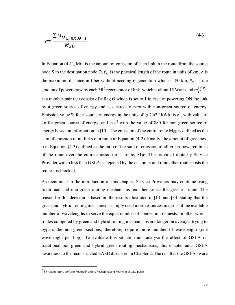
35
ρ=∑ 𝑀𝑖𝑗𝑖,𝑗 ∈𝑅 ,Θ=1
𝑀𝑆𝐷
(4-3)
In Equation (4-1), Mij is the amount of emission of each link in the route from the source
node S to the destination node D, ℓ𝑖𝑗 is the physical length of the route in units of km, ∧ is
the maximum distance in fiber without needing regeneration which is 80 km, 𝑃𝑅3 is the
amount of power draw by each 3R2 regenerator of link, which is about 15 Watts and 𝑚𝑖𝑗(𝛩,𝛹)
is a number-pair that consist of a flag Θ which is set to 1 in case of powering ON the link
by a green source of energy and is cleared to zero with non-green source of energy.
Emission value Ψ for a source of energy in the units of [g Co2 / kWh] is e1, with value of
26 for green source of energy, and is e2 with the value of 880 for non-green source of
energy based on information in [10]. The emission of the entire route MSD is defined as the
sum of emission of all links of a route in Equation (4-2). Finally, the amount of greenness
ρ in Equation (4-3) defined as the ratio of the sum of emission of all green-powered links
of the route over the entire emission of a route, MSD. The provided route by Service
Provider with ρ less than GSLA, is rejected by the customer and if no other route exists the
request is blocked.
As mentioned in the introduction of this chapter, Service Providers may continue using
traditional and non-green routing mechanisms and then select the greenest route. The
reason for this decision is based on the results illustrated in [13] and [34] stating that the
green and hybrid routing mechanisms simply need more resources in terms of the available
number of wavelengths to serve the equal number of connection requests. In other words,
routes computed by green and hybrid routing mechanisms are longer on average, trying to
bypass the non-green sections, therefore, require more number of wavelength (one
wavelength per hop). To evaluate this situation and analyse the effect of GSLA on
traditional non-green and hybrid green routing mechanisms, this chapter adds GSLA
awareness to the reconstructed EASB discussed in Chapter 2. The result is the GSLA aware
2 3R regenerators perform Reamplification, Reshaping and Retiming of data pulse.
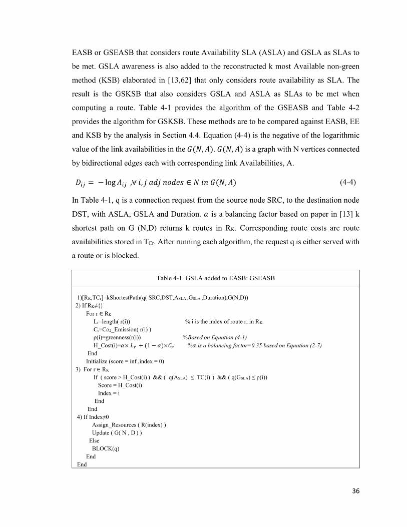
36
EASB or GSEASB that considers route Availability SLA (ASLA) and GSLA as SLAs to
be met. GSLA awareness is also added to the reconstructed k most Available non-green
method (KSB) elaborated in [13,62] that only considers route availability as SLA. The
result is the GSKSB that also considers GSLA and ASLA as SLAs to be met when
computing a route. Table 4-1 provides the algorithm of the GSEASB and Table 4-2
provides the algorithm for GSKSB. These methods are to be compared against EASB, EE
and KSB by the analysis in Section 4.4. Equation (4-4) is the negative of the logarithmic
value of the link availabilities in the 𝐺(𝑁, 𝐴). 𝐺(𝑁, 𝐴) is a graph with N vertices connected
by bidirectional edges each with corresponding link Availabilities, A.
𝐷𝑖𝑗 = − log 𝐴𝑖𝑗 ,⩝ 𝑖, 𝑗 𝑎𝑑𝑗 𝑛𝑜𝑑𝑒𝑠 ∈ 𝑁 𝑖𝑛 𝐺(𝑁, 𝐴) (4-4)
In Table 4-1, q is a connection request from the source node SRC, to the destination node
DST, with ASLA, GSLA and Duration. 𝛼 is a balancing factor based on paper in [13] k
shortest path on G (N,D) returns k routes in RK. Corresponding route costs are route
availabilities stored in TCr. After running each algorithm, the request q is either served with
a route or is blocked.
Table 4-1. GSLA added to EASB: GSEASB
1)[RK,TCr]=kShortestPath(q( SRC,DST,ASLA ,GSLA ,Duration),G(N,D))
2) If RK≠{}
For r ∈ RK
Lr=length( r(i)) % i is the index of route r, in RK
Cr=Co2_Emission( r(i) )
ρ(i)=greenness(r(i)) %Based on Equation (4-1)
H_Cost(i)=𝛼× 𝐿𝑟 + (1 − 𝛼)×𝐶𝑟 %𝛼 is a balancing factor=0.35 based on Equation (2-7)
End
Initialize (score = inf ,index = 0)
3) For r ∈ RK
If ( score > H_Cost(i) ) && ( q(ASLA) ≤ TC(i) ) && ( q(GSLA) ≤ ρ(i))
Score = H_Cost(i)
Index = i
End
End
4) If Index≠0
Assign_Resources ( R(index) )
Update ( G( N , D ) )
Else
BLOCK(q)
End
End

37
Table 4-2. GSLA added to KSB: GSKSB
1) [RK,TCr]=kMostAvailablePath (q(SRC , DST, ASLA , GSLA , Duration),G(N,D))
2) If RK≠{}
For r ∈ RK
ρ(i)=greenness(r); %Based on Equation (4-1)
End
Initialize (score = inf ,index = 0)
3) For r ∈ RK
If ( q(ASLA) ≤ TCr(i) ) && ( q(GSLA) ≤ ρ(i))
Score = GNr
Index = ri
End
End
4) If Index≠0
Assign_Resources ( R(index) )
Update ( G( N , D ) )
Else
BLOCK(q)
End
End
4.3.2. Effect of Adopting Green SLA in “Greener Networks” on the Value of Key
Performance Metrics of WDM Networks
This section of the analysis studies the effect of adopting GSLA on a network that on
average has more available green energy. This means that the links of a network will be
powered ON by green energy for longer duration. The analysis in Section 4.3.1 of this
chapter is based on the network that has a random and equal chance of selecting the energy
sources for links in the simulation part of the analysis. We define a new system with two
states for each link of the network. Two states are 1, a link is using the green source of
energy, and 2, link is using the non-green source of energy. By defining a one-step two-
by-two Markov matrix S(i,j) for this system in Figure 4-1, we determine the chance of
being in each state in the next step of time. The next step of time in our analysis is the 6
hours emission topology change interval in which another source of energy is randomly
assigned to all links of a network. In this matrix, P11 is probability of staying in state 1
(using green energy again) and P12, is probability of going from state 1 to 2 (using non-
green energy when currently using green energy). P21 is probability of going from state 2
to 1 (using green energy next when currently using non-green energy), and P22 is remaining
in state 2 or using non-green energy for the next 6 hours when currently using non-green
energy. If P11 > P12 then there is a higher chance of having green energy or staying in state
38
1, (again) for the next 6 hours. Similarly, if P21 > P22 then there is a higher chance of going
from non-green energy to green energy in the next step. For simplicity, we will equate P11
and P21. Therefore, P12 and P22 will be the same as well. Each link has a corresponding
matrix, and all P values are zero when there is no connectivity between nodes, as shown in
Equation (4-5). For the sake of consistency, we will consider the same probability values
for all the links of a network. With this setup, we can say that all the links of a network
have the same chance of having green energy with P11 and P21. The next section details the
condition in which re-provisioning may affect the GSLA Satisfaction, (GSLS).
Figure 4-1. Two states of the link energy
𝑠(𝑖,𝑗)={[𝑃11 𝑃12
𝑃21 𝑃22]
⩝ 𝑖, 𝑗 𝑎𝑑𝑗 𝑛𝑜𝑑𝑒𝑠 ∈ 𝐺(𝑁, 𝐸))
[0 00 0
] ⩝ 𝑖, 𝑗 𝑛𝑜𝑛 − 𝑎𝑑𝑗 𝑛𝑜𝑑𝑒𝑠 ∈ 𝐺(𝑁, 𝐸) 𝑜𝑟 𝑖 = 𝑗
(4-5) Two-by-two Markov matrix for each link
4.3.3. The Effect of Re-Provisioning on Green SLA Satisfaction
In this chapter, we also analyse the effect of re-provisioning of the established lightpaths
in the case of a change in the topology of a network. The type of topology change
considered in this chapter is the energy and emission topology change for links of the

39
network. The type of energy (green or non-green) is changed every topology change
interval (6 hours in this chapter). Re-provisioning tries to reroute and re-provision the
established lightpaths that may not be optimized and emit more emission. This is because
with emission topology change, established routes may be passing through links that are
not green energy powered anymore and emit more GHGs. With emission topology change
a new route may be computed for the already established route that may not meet the
GSLA. For this analysis the adaptive routing mechanism in [30]is considered. Adaptive
EASB (A-EASB) re-provisions the established route by replacing the route with one that
has lower hybrid cost. We will show that re-provisioning does not change GSLA
satisfaction by a considerable amount. Table 4-3 presents the reconstructed re-provisioning
algorithm of the Adaptive EASB (A-EASB) in the form of a pseudocode.
Table 4-3. Re-Provisioning with A-EASB
If Topology_change_Flag=1
For e=1 to #Established_connections
S= Established_connections (e )
[SRC, DST, ASLA ,H_CostS]=get_Characteristic( S ) %S, D, Availability of route, Hybrid cost, current route
[R,TCr]=kShortestPath(S( SRC,DST,ASLA ),G(N,D)) %Array of routes R, and Array of associated total costs
(or route availabilities), TC
If R≠{}
For r∈ R
Lr=length( r( i )) % i is the index of route r, in R
Cr=Co2_Emission( r(i) ) %With new emission topology info after emission
topology change
GNr=greenness( r(i) ) %Based on Equation (4 1)
H_Cost( i ) =𝛼× 𝐿𝑟 + (1 − 𝛼)×𝐶𝑟 %𝛼 is a balancing factor=0.35 based on Equation (2-7)
End
Initialize (score = inf ,index = 0)
For r ∈ R
If ( score > H_Cost( i )) && ( S(ASLA) ≤ TC( i ) ) )
Score = H_Cost( i ))
Index = i
End
End
IF ( ( (H_CostS– H_Cost(i) / H_CostS) ≥ 0) )
Assign_Resources ( R(i) )
Release ( SP )
Update ( G( N , D ) )
End
End
End
End
40
4.4. Analysis
4.4.1. Simulations Network
The network used for the analysis section of this chapter is the network of NSFNet shown
in Figure 4-2 with 14 nodes and 21 bidirectional links. The numbers on the links represent
the actual physical distance between nodes in km. The network consists of the two layers
of data and control planes of GMPLS networks. The regenerators of the optical links
amplify the entire “band” based on [11] and therefore are considered either ON or OFF
with no intermediate value for the energy used. The data plane has 96 available to assign
wavelengths or Lambdas in WDM fashion without the continuity constraint based on the
analysis in [39]. The availability of the optical links is randomly assigned a number from
0.999 to 0.99995 and is assumed constant for the entire duration of simulations. The two
types of the energy sources can randomly turn ON the links of the network, and every 6
hours of the simulated time the type of energy is randomly reassigned again for all links,
which is the emission topology change interval in this chapter. The two types of energy are
a green source of energy with an average of 26 gCo2/ kWh for the green source of energy
and 880 gCo2/kWh for a non-green source of energy according to the document in [10].
The arrival of the connection requests is a Poisson process and follows an exponential
distribution with the arrival rate of 10 connections per hour for the first scenario and 100
connections per hour for the second scenario. Duration or hold time of the connections also
follows the exponential distribution with a mean value of 10 hours. The amount of load is
defined as the product of connection arrival rate and connection duration in units of Erlang
as illustrated in [63]. Therefore, scenario 1 is rated as 100 Erlang and Scenario 2 as 1000
Erlang. The requested route availability (ASLA) by connection requests ranges from 0.99
to 0.9995 for all sections of the analysis. The network model has been built in MATLAB
programming language. All simulations take advantage of parallel computing toolbox of
MATLAB which can use compute clusters.

41
Figure 4-2. NSFNet Network
4.4.2. Variables and Performance Metrics
This section details the important variables and defines various performance metrics for
each section of the analysis. The first metric is the resource efficiency, which is the average
number of Lambdas (hops) per lightpath, for each route. Depending on the routing
mechanism used, this value may be different. The lower value for this metric is preferable
for Service Providers. Higher average for this metric means that more Lambdas must be
provisioned on average to establish the equal number of connection requests. The second
metric is the reduction in emission in terms of average gram Co2 per unit resource Lambda.
This metric is the emission in power generation to turn ON regenerators of a link. This
parameter determines how well green sections are used. The lower the average emission,
the more green-sections used in the optical networks. The third parameter is the success
rate in serving connection requests, which is the ratio of the number of served connections
over a total number of connection requests. Since SLAs must be met to assign a route for
a connection request, some requests may be blocked because there may not be any route
that satisfies the SLA(s) of the connection request. The other reason to decrease the success
rate (or increase the blocking rate) is the fact that an optical network may be overwhelmed
by a huge number of requests and run out of resources or available-to-assign wavelengths
(Lambdas), as we will see in scenario 2. The fourth parameter is the GSLA satisfaction
which is the ratio of the connection requests that were served with a route that met or
exceeded their GSLA value to the total number of the server connection. Route Availability

42
SLA satisfaction resulted in 100 % for both scenarios in this work and was not graphed.
Section of 4.2 will detail the levels of variables used for analysis.
4.4.3. Analysis on the Effect of Adopting GSLA
In this section EE, EASB, GSEASB, KSB and GSKSB are analysed and benchmarked
against the four performance metrics detailed in Section 4.2. This section of analysis
considers Scenario 1 and Scenario 2. EASB and KSB only consider ASLA, and GSEASB
and GSKSB consider ASLA and GSLA. EE is an exception with no SLA requirement.
GSLA required by connection request ranges from 10 to 20 %. In this section P11 =P21=
50.
4.4.4. Effect of GSLA in “Greener” Network
For this part of the analysis P11 =70 % or 0.7 is used to increase the chance of having green
energy in an optical network. As mentioned in section 3.2, P11 = P21 and P12 = P22. For this
section, GSLA of 10 to 80 % (heavier GSLA) is proposed to see the effect of a greener
network. Both Scenario 1 and Scenario 2 are considered in this section. It is expected that
GSLA satisfaction and success rate will increase even with the higher maximum GSLA
value. (compared to maximum 20 % GSLA of Section 4.2.1.)
4.4.5. Analysis on the Effect of Re-provisioning on GSLA
For this section, Adaptive EASB (A-EASB) is considered with all other routing mechanism
in the previous sections of analysis. The amount of greenness or GSLA is also considered
from 10 to 20 % as maximum possible GSLA values. For this section, the Scenario 2 is
analysed only, as there is a higher chance of GSLA satisfaction violation and variation with
heavy traffic. In this section only the success rate and GSLA satisfaction are analysed. This
section uses the network of Section 4.2.1 with P11 = 50 %.
4.5. Results of Analysis
4.5.1. Effect of Adopting Green SLA
For emission reduction with light traffic intensity of scenario 1 in Figure 4a, as expected
EE has the lowest average emission per unit resource lambda and forms the lower bound

43
of Figure 4-3. KSB as the non-green method has the highest average emission and is the
upper bound. The adoption of GSLA by KSB and EASB reduced the average emission per
unit resource Lambda as seen in Figure 4-3. GSKSB has about 10 to 15 % lower emission
as compared to KSB and GSEASB has close to 5 % less emission compared to EASB.
Figure 4a indicates that selecting the greener route (not surprisingly) lowers the emission
However, as we will see in later figures this comes at a cost. Figure 4-4 shows the situation
for the emission reduction with the Scenario 2 when traffic is heavy. As seen in Figure 4-4,
with the heavy traffic there is no significant reduction in emission and all the routing
mechanisms perform almost the same. The difference between the worst and the best is
scatted over only 5 %. This is because all the links of the network will be turned ON to
accommodate the heavy traffic and no link even turned ON by a non-green source of energy
will be turned OFF. For resource efficiency and scenario 1 in Figure 4-5, as expected, EE
has the highest average resource utilization (Lambda per connection or lightpath) and KSB
has the lowest average resource per connection. This means connections or lightpaths
established by EE are longer (in unit of hops) on average and require more Lambda or
resources. Based on Figure 4-5, the price to pay for having lower emission with GSKSB
and GSEASB is the significant increase in resource utilization level. GSKSB is 0.5 hops
longer on average compared to KSB which is more than 20 %. So, to decrease the emission
by 10 to 15 %, GSKSB increased the resource utilization by more than 20 %. This behavior
is repeated for EASB. GSEASB has more than 10 % higher resource utilization and longer
connections to reduce the emission by 5 %. The hybrid method EASB averages at more
reasonable value and has lower resource utilization for connections compared to GSEASB
and GSKSB. The resource efficacy is even worse for GSEASB and GSKSB when traffic
is heavy (in Scenario 2) as seen in Figure 4-6. Figure 4-6 shows that GSKSB and GSEASB
have even higher resource utilization than EE and consume the most of the resources. This
situation with GSKSB and GSEASB is highly unwanted, because as we saw in Figure 4-4
all routing mechanism performed almost the same in terms of the emission reduction. As
seen in Figure 4-6 there is an increase on average resource utilization of all routing
mechanisms that consider the route availability ASLA (EASB, KSB, GSEASB and
GSKSB). This is due to the fact that with high traffic and utilization of all optical links of
a network, some connections may need to travel longer (and less reliable) routes to be able

44
to accommodate the availability requested by a connection. GSKSB and GSEASB will
need to satisfy the GSLA with longer routes as well, that may be less green (ρ is small).
EE does not consider any SLA and therefore does not behave in similar fashion. For GSLS
in Figure 4-7 and Figure 4-8, GSKSB and GSEASB provided 100 % satisfaction for the
requests that they “served” as they considered the GSLA in finding the route for a
connection request. In Figure 4-7, the routing based on energy parameters with EE resulted
in about 95 % GSLA satisfaction which is very interesting to note. The interesting fact
about this observation is that, even with the EE method and routing solely based on energy
and emission parameters, there is no way to provide 100 % GSLA satisfaction even for a
very low maximum of 20 % GSLA value. This obesevation suggests increasing investment
on green energy infrastructure for optical networks. EASB provides about 10 % more
satisfaction as compared to the non-green routing mechanism KSB. In Figure 4-8 for the
Scenario 2, the GSLA satisfaction becomes almost the same for all non-GSLA aware
routing mechanisms again due to the high volume of traffic higher utilization of all links
with higher ρ. It is interesting to note that EE and EASB have a significant drop in GSLA
satisfaction. With the higher value of utilization of links, using non-green links and not
considering GSLA, there is a higher chance of violating a GSLA, as seen in Figure 4-8.
Figure 4-9 presents the network blocking rate or connection success rate in the Scenario 1.
As seen in this figure, with low to moderate traffic and the maximum requested GSLA of
20 %, the adoption of GSLA did not decrease the success rate. Based on Figure 4-9 all
routing mechanism provide almost equal success rate for connection requests even by
having higher or lower resource efficiency as seen in Figure 4-5. However different results
are seen for scenario 2 in Figure 4-10. As expected, adding GSLA decreased the success
rate of the network not just because GSEASB and GSKSB have higher average resource
utilization as seen in Figure 4-6, but also because they have to consider GSLA as well.
When there is a contention for resources with heavy traffic of scenario 2, the addition of
GSLA adds another constraint in finding a route for GSEASB and GSKSB, which translate
into even more “failure” (or blocking connection request). In Figure 4-10 EASB and KSB
perform better than GSLA aware mechanisms. EE also has a lower success rate when
compared to EASB and KSB, again because of the higher resource utilization. Figure 4-11
in analysis of this section is a figure for scenario 1 when the maximum GSLA value is 80

45
%. As we can see in Figure 4-11, the success rate for GSEASB and GSKSB is dropped by
15 %, even for the light traffic, which is not acceptable. In this figure GSKSB and GSEASB
overlap, clearly indicating that the decrease in success rate is due to the adoption of GSLA.
Based on our analysis in this section, the addition of GSLA to routing mechanisms
increases the resource utilization for both scenarios, while there is no similar or better
reduction in emission. In the case of light traffic, there may be no problem (although highly
undesired) with an increase in resource utilization because the blocking rate of the network
remains about 1 %. However, the blocking rate of the network is increased significantly
with GSEASB and GSKSB in scenario 2. It is fair to assume that the usage of green and
hybrid routing mechanisms (EE and EASB) may be more preferred by Service Providers
because of the lower resource utilization and higher success rate when maximum greenness
required (GSLA value) is about 20 %. The links of the current network in this section are
turned ON by random sources of energy with equal probabilities. In the next section, we
will consider the same 80 % maximum GSLA analysis for a network that on average is
about 20 % greener compared to the simulated network of this section.
Figure 4-3. Average emission per Lambda
analysis (Scene 1)
Figure 4-4. Average emission per Lambda analysis
(Scene 2)

46
Figure 4-5. Average connection length analysis
(Scene 1)
Figure 4-6. Average connection length analysis
(Scene 2)
Figure 4-7. GSLA satisfaction analysis (Scene 1)
Figure 4-8. GSLA satisfaction analysis (Scene 2)
Figure 4-9. Success rate analysis (Scene 1) Figure 4-10. Success rate analysis (Scene 2)

47
Figure 4-11. Success rate in scenario 1 with up 80% GSLA value analysis (Scene 1)
4.5.2. Effect of Adopting GSLA in Greener Networks on Optical Network Parameters
This section of analysis shows the results for performance metrics when the green source
of energy has 20 % more chance (P11 =70) of turning ON the links of the network for both
Scenarios 1 and Scenario 2. The maximum GSLA value for this section is 80 %.
As we can see from Figure 4-12 for Scenario 1, KSB and EE have the maximum and
minimum emission respectively similar to Figure 4-3 However, not surprisingly the
emission has been dropped by 30 units (gram Co2 per Lambda), for almost all routing
mechanisms in Figure 4-12. GSKSB has reduced the emission of KSB by about 25 %. This
is a significant drop in emission by GSKSB and it is possible because GSKSB has more
chance of finding a greener route on average since the network itself is greener. GSEASB
also reduced the emission of EASB by about 12 %. This reduction is less than that of
GSKSB because EASB itself is already a green aware and hybrid routing mechanism
giving already lower emissions per unit resource. Results of the analysis for Scenario 2 in
Figure 4-13 reveals that in heavy traffic conditions, the best and worst routing mechanisms
are separated by12 %. This difference as mentioned in the last section, is because all
sections of the network are turned ON. The surprising fact about Figure 4-13 is that
GSEASB and GSKSB have lowest average emission per unit resource, however, the reason
for this behavior is determined by considering Figure 4-19. When the amount of resources
is limited, the success rate of GSEASB and GSKSB is close to only 57 %, therefore, they
Days
0 5 10 15 20 25 30 35 40
Su
scess R
ate
in %
0.7
0.75
0.8
0.85
0.9
0.95
1
EASBEEGSEASBKSBGSKSB

48
“fail” or block more connection requests and use more resources to find the greener paths
for the requests they serve.
Resource efficiency of Figure 4-14 for the Scenario 1 almost repeats the results of Figure
4-5 with EE having the highest and KSB having the lowest average resource utilization.
As we can see in Figure 4-14, even with greener network GSKSB and GSEASB increase
the average resource usage. In this figure GSKSB with 14 % increase in average hop length
compared to KSB becomes almost similar to the performance of EASB with greener
network. However again EASB has lower emission as seen in Figure 4-12. GSEASB
increases the resource utilization of EASB by 8 %. In Figure 4-15 and with heavy traffic
of scenario2, the same overall increase in average resource utilization is observed again
but as expected this increase is smaller compared to results of Figure 4-6. GSEASB has the
most resource utilization, increasing the average connection length of EASB by 13 %. This
is close to half of the 24 % increase in Figure 4-6 due to increase in existence of green
links. GSKSB performed almost the same as EE in long run which questions the usage of
GSKSB again considering the fact that GSKSB has lower success rate again as we will see
in Figure 4-19.
GSLA satisfaction in Figure 4-16 for scenario 1 has an overall increase compared to Figure
4-7 especially for EE which gets close to 100 %. For EE this is about 98 % for GSLA of
up to 80 % (as opposed to 95 % with 20 % GSLA value). As expected, GSKSB and
GSEASB have 100 % satisfaction, because they consider the GSLA in finding the route
for connection requests. EASB also has about 5 % increase from the one in Figure 4-7 and
is close to 90 % for 80 % maximum GSLA, which is a considerable improvement. KSB as
the non-green method has no increase in GSLA satisfaction. Increased chance of having
green sources of energy in this analysis did not increase the overall GSLA satisfaction of
EE, EASB and KSB as seen in Figure 4-17 for scenario 2. Except for GSKSB and
GSEASB, all routing mechanisms provided the same GSLA satisfaction of close to 75 %
which is close to GSLA satisfaction of KSB as a non-green method. This is no surprise
because again with the limited number of resources and trying to serve as many connection
requests as possible. EE and EASB tend to behave like KSB by using all the remaining,
perhaps non-green links and therefore decreasing the GSLA satisfaction.

49
The Result of our analysis for the success rate of routing mechanisms is reflected in Figure
4-18 and Figure 4-19. Figure 4-18 repeats the results of Figure 4-9 with almost 100 %
success rate for EE, EASB, and KSB for Scenario 1 in Figure 4-18. We observe about 10
% increase in the success rate of GSKSB and GSEASB compared to Figure 4-11. By
increasing the probability of using the green energy by 20 % the success rate of GSEASB
and GSKSB increase by 10 % to about 97 % which may be acceptable for GSLA values of
up to 80 %. For Scenario 2, the overall success rate shows about 2 % increase for GSKSAB
and GSEASB. Although no significant change is observed for success rate of the routing
mechanisms when compared to Figure 4-10, but we have to be reminded again that Figure
4-19 shows the same results as compared to Figure 4-10, but for GSLA of up to 80 % as
opposed to the 20 % maximum GSLA value of the Figure 4-10. Figure 4-19 shows that
GSEASB and GSKSB increase the blocking rate of the EASB and KSB by 10 %
respectively.
Based on our analysis in this section, it is possible to conclude that adoption of GSLA by
traditional non-green routing mechanism and hybrid routing mechanism increases the
average resource utilization and the blocking rate of a network. The amount of reduction
in the average emission per unit resource does not justify the amount of increase resource
utilization. A 10 % decrease in the success rate of a network when traffic is heavy translated
in net 10 % loss of income for Service Providers. The next section will consider the effect
of “adaptivity” in case of emission topology change in a network that has an equal chance
of having a green or non-green source of energy for optical links.
Figure 4-12. Average emission per Lambda
analysis (Scene 1, max GSLA of 80%)
Figure 4-13. Average emission per Lambda
analysis (Scene 2, max GSLA of 80%)

50
Figure 4-14. Average connection length analysis
(Scene 1, max GSLA of 80%)
Figure 4-15. Average connection length analysis
(Scene 2, max GSLA of 80%)
Figure 4-16. GSLA satisfaction analysis (Scene 1,
max GSLA of 80%)
Figure 4-17. GSLA satisfaction analysis (Scene 2,
max GSLA of 80%)
Figure 4-18. Success rate analysis (Scene 1, max
GSLA of 80%)
Figure 4-19. Success rate analysis (Scene 2, max
GSLA of 80%)

51
4.5.3. Results of Analysis on The Effect of Re-provisioning on GSLA Satisfaction
In this section, we analyse the effect of re-provisioning or rerouting the established
lightpaths in case of emission topology change with Scenario 2 on GSLA satisfaction rate.
lower GSLAS is anticipated, because, as mentioned in Section 3.3, rerouting the routes
without considering the GSLA may replace a currently established route that satisfies the
GSLA of a request with a new route that does not satisfy the GSLA of the request. If a
lightpath is marked for reprovisioning as a result of emission topology change, it may also
be in violation of the GSLA after the emission topology change. We are interested to know
the percentage drop in satisfaction. The average emission per unit resource for Adaptive-
EASB (A-EASB) was slightly less as compared to EASB in Figure 4-4. The average
resource utilization resulted the same outcome as Figure 4-6 with slightly less resource
utilization for A-EASB when compared to EASB and they were not graphed.
As we can see in Figure 4-20, the A-EASB reduced the GSLA satisfaction rate. However
the difference between the EE and A-EASB is about 5 %. This is very important, because
a significant drop in GSLA satisfaction could have happened because of high intensity of
the traffic in Scenario 2 when compared to other non-GSLA aware routing mechanisms.
Therefore, we can conclude that emission topology change drops the GSLA satisfaction
only up to 5 %. Obviously, GSEASB and GSKSB have the 100 % satisfaction here again.
The drop in GSLA satisfaction is only 5 %, but by looking at Figure 4-21 we realize that
A-EASB provides more than 10 % increase in success rate or lower blocking rate as
compared to EE and 15 % or more success rate as compared to GSEASB.
Figure 4-20. GSLA satisfaction analysis (Scene 2)
with adaptive method
Figure 4-21. Success rate analysis (Scene 2) with
adaptive method

52
4.6. Conclusion and Future Work
This chapter presented GSLA awareness for the hybrid and traditional routing mechanisms
and the effect of the adoption of GSLA on a network through proposed mathematical
models and algorithms. The discussion on the results of the analysis in this chapter had
successfully showed that adopting GSLA by routing mechanisms decreased the resource
efficiency with both light and heavy traffic in return for less reduction in emission as
compared to green and hybrid routing mechanisms. It was also obvious that in the case of
light traffic, there may be no problem with this increase in resource utilization, because the
success rate of the network remains high. The success rate of network was decreased with
GSEASB and GSKSB methods due to higher resource usage and utilization. It was
reasonable to assume that the usage of green and hybrid routing mechanisms such as EE
and EASB may be more preferred by Service Providers because of a lower resource
utilization and a higher success rate. The drop in Green SLA Satisfaction is only 5 % for
Adaptive-EASB compared to other non-GSLA aware routing mechanisms in return for 5
to 15 % success rate compared to GSEASB. Adaptive EASB was a reasonable choice for
Service Providers to increase the success rate of networks without sacrificing the GSLA
satisfaction by a considerable amount. In a nutshell. The results revealed that adopting the
GSLA by routing mechanisms decreased the resource efficiency with both light and heavy
traffic in return for less reduction in emission as compared to green and hybrid routing
mechanisms.
The future work will study the effect of different values for GSLA violation that may
change the decision of Service Providers. The amount of extra energy used by GSEASB
and GSKSB will also be determined in the case of light and intensive traffic loads on optical
networks. Although the green parameters used in this chapter are specific to Link State
Routing mechanisms, but they very well can be disseminated as Path Attributes using
Border Gateway Protocol (BGP) just like the papers in [64,65]. A part of future work will
also study the effect of greening the autonomous systems and the effect of GSLA adoption
on path selections.
53
Chapter 5 MULTI-SLA AWARE CONSTRAINED LOWEST
EMISSION FIRST
5.1. Introduction
This chapter presents the extended version of the paper published in [15]. This chapter
presents a Multi-SLA aware routing mechanism which considers ASLA and DSLA of the
connection request. The new routing mechanism of this chapter as well as the other routing
mechanisms introduced in Chapter 2 as foundation work have been reconstructed and
tested with a set of realistic energy and emission information. This chapter is organized as
follows: Section 5.2 gives the chapter specific related work. Section 5.3 introduces the new
routing mechanism as well as introducing the realization of DSLA and the method to
generate the realist energy and emission data. Section 5.4 formulates a non-green routing
mechanism to be tested along with other routing methods in the analysis section. Section
5.5 reviews the testbed environment and reviews the performance metrics used in this
chapter. Section 5.6 presents the results of two types of analysis performed to ensure the
performance of the proposed routing method followed by Section 5.7 that concludes the
chapter and states the future work. chapter specific related work comes next
5.2. Related Work
Unfortunately, when it comes to developing a new routing method for Green networks, the
role of many service parameters such as Service Level Agreements (SLAs) is ignored.
Green routing mechanisms in [11,12,14,34,45,51,66,67] have not considered any SLAs in
the operation of the proposed Green routing methods. Not considering the SLAs makes the
green mechanisms less favorable and less practical. The other major issue in the
development of green routing mechanism is the inaccuracy of the testing environment for
Green networks as also mentioned in Section 1.2. Benchmarking the new Green methods
is not performed using accurate energy and emission information. Many papers such as
[11-14,23,68] have considered the source of energy to be either 100% green or 100% non-
green which is not the case in practice.
The routing method on this chapter relies on the propagation of the energy greenness
parameters with a new Link State Advertisement (LSA) introduced in [69] for Link-State

54
type Routing and Traffic Engineering (TE) mechanisms. In this chapter, a lightpath transits
each node either transparently (with no extra energy) or by Lambda conversion using two
transponders, similar to the setup in [15,70]. Power draw by two transponders is 170 Watts
as explained in Table 2-1 from [48]. In this chapter, the inline amplifiers and signal leveling
amplifiers are considered either ON or OFF and regenerate the entire spectrum (lightpaths)
with no intermediate value as also explained in [11].
5.3. Multi-SLA Aware Constrained Least Emission First (CLE)
Before introducing the routing mechanism, it is beneficial to introduce the energy and
emission related information used with the new method.
5.3.1. Energy and Emission Data
As mentioned earlier, the energy powering each section of the network is composed of
different sources as shown in Figure 5-1, from the webpage in [71] for the province of
Ontario in Canada. Each source of energy has a different value of emission as detailed in
[10]. In general, coal and petroleum have the highest amount of emission e.g. 880 to 980
[g Co2 per kWh]. The amount of emission for green sources of energy such as the wind
and hydro is considered zero.
Figure 5-1. Different source of energy in province of Ontario
When performing the analysis, no single source would provide the information about the
generation capacity for each section of the simulated testbed, which spans the United
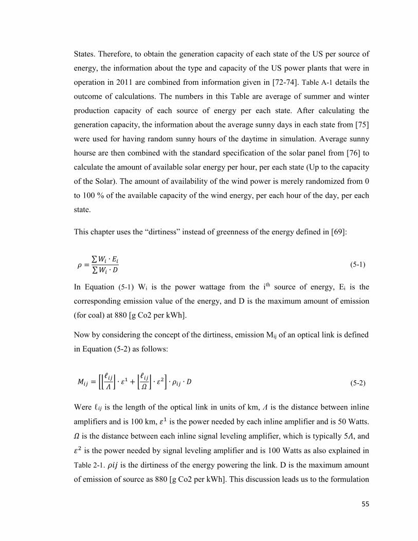
55
States. Therefore, to obtain the generation capacity of each state of the US per source of
energy, the information about the type and capacity of the US power plants that were in
operation in 2011 are combined from information given in [72-74]. Table A-1 details the
outcome of calculations. The numbers in this Table are average of summer and winter
production capacity of each source of energy per each state. After calculating the
generation capacity, the information about the average sunny days in each state from [75]
were used for having random sunny hours of the daytime in simulation. Average sunny
hourse are then combined with the standard specification of the solar panel from [76] to
calculate the amount of available solar energy per hour, per each state (Up to the capacity
of the Solar). The amount of availability of the wind power is merely randomized from 0
to 100 % of the available capacity of the wind energy, per each hour of the day, per each
state.
This chapter uses the “dirtiness” instead of greenness of the energy defined in [69]:
𝜌 =∑ 𝑊𝑖 ∙ 𝐸𝑖
∑ 𝑊𝑖 ∙ 𝐷 (5-1)
In Equation (5-1) Wi is the power wattage from the ith source of energy, Ei is the
corresponding emission value of the energy, and D is the maximum amount of emission
(for coal) at 880 [g Co2 per kWh].
Now by considering the concept of the dirtiness, emission Mij of an optical link is defined
in Equation (5-2) as follows:
𝑀𝑖𝑗 = [⌊ℓ𝑖𝑗
𝛬⌋ ∙ 휀1 + ⌊
ℓ𝑖𝑗
𝛺⌋ ∙ 휀2] ∙ 𝜌𝑖𝑗 ∙ 𝐷 (5-2)
Were ℓ𝑖𝑗 is the length of the optical link in units of km, Λ is the distance between inline
amplifiers and is 100 km, 휀1 is the power needed by each inline amplifier and is 50 Watts.
𝛺 is the distance between each inline signal leveling amplifier, which is typically 5𝛬, and
휀2 is the power needed by signal leveling amplifier and is 100 Watts as also explained in
Table 2-1. 𝜌𝑖𝑗 is the dirtiness of the energy powering the link. D is the maximum amount
of emission of source as 880 [g Co2 per kWh]. This discussion leads us to the formulation

56
of emission of a route Msd, connecting source node s to destination node d in Equation
(5-3):
𝑀𝑠𝑑 = ∑ 𝑀𝑖𝑗
∀ 𝑖,𝑗∈𝑅
+ {휀𝑠4 ∙ 𝜌𝑠 + 휀𝑑
4 ∙ 𝜌𝑑 + 휀𝑗∉(𝑠,𝑑)3 ∙ 𝜌𝑗} ∙ 𝐷 (5-3)
In which 휀𝑠4 is the power needed to add a Lambda in source node s, 𝜌𝑠 is the dirtiness of
energy turning ON the node s, 휀𝑑4 is the energy needed for dropping a Lambda at destination
node d, multiplied by 𝜌𝑑which is the dirtiness of energy at destination node d. 휀𝑗∉(𝑠,𝑑)3 is
the energy needed for Lambda conversion, (if needed) in a transit node which is multiplied
by corresponding dirtiness 𝜌𝑗. Energy for adding and dropping of the Lambda at source
and destination nodes are the constant part of the energy needed to establish a lightpath.
The strategy for minimizing the emission in this chapter is to reduce the variable energy
usage in nodes by minimizing the Lambda conversions, and by using greener links for
establishing the lightpaths. In this chapter as explained in Section 2.5, power reduction and
optimization is performed for the optical layer only.
5.3.2. Realization of Delay SLA
Per information in [77], the maximum end-to-end delay of the North American network of
NTT DATA Service Provider is 50 ms. The 50 ms is divided over four time zones,
representing the distances between nodes, similar to the approach in [14]. Therefore,
traversing through each zone should add a maximum of 12.5 ms to the overall end-to-end
delay of the route. The information about the time zones is depicted in Figure 5-2. from
World Atlas website in [78]. The zone information is overlaid with the node and link
locations shown in Figure 5-3. from [79]. Based on the combined view of Figure 5-2. and
Figure 5-3 the Delay SLA (DSLA) of any connection or lightpath from node 1 to node 3
(entirely in zone 1) and node 1 to node 7 (through 3 zones) could not be more than 12.5 ms
and 37.5 ms, respectively. This chapter uses non-coherent transponders with no Forward
Error Correction (FEC) based on information in [80] which have a delay in units of Nano
seconds, therefore delay at each node is about 10 ms if Lambda conversion is performed
based on information in [80]. The link delay Tij is simply a division of physical length of
the link by the speed of the light in a vacuum.
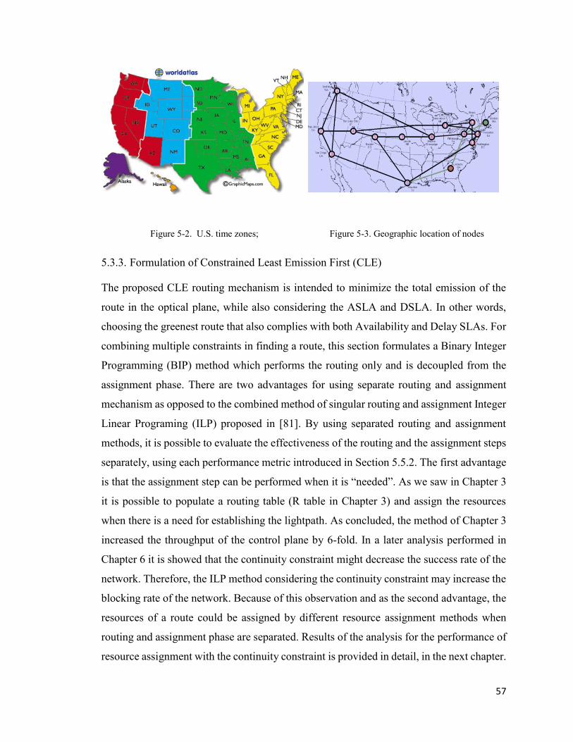
57
Figure 5-2. U.S. time zones; Figure 5-3. Geographic location of nodes
5.3.3. Formulation of Constrained Least Emission First (CLE)
The proposed CLE routing mechanism is intended to minimize the total emission of the
route in the optical plane, while also considering the ASLA and DSLA. In other words,
choosing the greenest route that also complies with both Availability and Delay SLAs. For
combining multiple constraints in finding a route, this section formulates a Binary Integer
Programming (BIP) method which performs the routing only and is decoupled from the
assignment phase. There are two advantages for using separate routing and assignment
mechanism as opposed to the combined method of singular routing and assignment Integer
Linear Programing (ILP) proposed in [81]. By using separated routing and assignment
methods, it is possible to evaluate the effectiveness of the routing and the assignment steps
separately, using each performance metric introduced in Section 5.5.2. The first advantage
is that the assignment step can be performed when it is “needed”. As we saw in Chapter 3
it is possible to populate a routing table (R table in Chapter 3) and assign the resources
when there is a need for establishing the lightpath. As concluded, the method of Chapter 3
increased the throughput of the control plane by 6-fold. In a later analysis performed in
Chapter 6 it is showed that the continuity constraint might decrease the success rate of the
network. Therefore, the ILP method considering the continuity constraint may increase the
blocking rate of the network. Because of this observation and as the second advantage, the
resources of a route could be assigned by different resource assignment methods when
routing and assignment phase are separated. Results of the analysis for the performance of
resource assignment with the continuity constraint is provided in detail, in the next chapter.

58
The BIP formulation of the CLE for minimizing the emission of the route while being SLA
compliant is presented in Equation (5-4) as follows:
𝑚𝑖𝑛 𝑀𝑅 = ∑ ∑ 𝑀𝑖𝑗 ∙ 𝑥𝑖𝑗
𝑗𝑖
(5-4)
Subject to:
− ∑ ∑(ln 𝐴𝑖𝑗 ∙ 𝑥𝑖𝑗)
𝑗𝑖
≥ −ln (𝐴𝑆𝐿𝐴) (5-5)
∑ ∑ 𝑇𝑖𝑗 ∙ 𝑥𝑖𝑗 ≤
𝑗𝑖
𝐷𝑆𝐿𝐴 (5-6)
All classical flow conservation shortest path problem constraints (5-7)
𝑥𝑖𝑗 = {1 𝑖𝑓 𝑙𝑖𝑛𝑘𝑠 𝑖𝑠 𝑢𝑠𝑒𝑑 0 𝑖𝑓 𝑙𝑖𝑛𝑘 𝑖𝑠 𝑛𝑜𝑡 𝑢𝑠𝑒𝑑
(5-8)
𝑥𝑖𝑗 + 𝑥𝑗𝑖 ≤ 1 ,⩝ i,j (5-9)
Equation (5-4) is the objective function to minimize the link emission of route R. Reduction
of emission in nodes can be achieved when assigning the resources of the router with
minimum Lambda conversion as elaborated in the analysis section. Equation (5-5) is the
first constraint that enforces the ASLA. Equation (5-6) is the second constraint that
enforces the DSLA. To save space, Equation (5-7) combines all (14 in this case) classical
flow conservation constraints of the Shortest Path problem. Equation (5-8) forces the
variable xij to be binary therefore if the link between node i and j is used, the xij is 1.
Otherwise, it is 0. Equation (5-9) is a simple sub-tour elimination constraint that makes
sure there is no loop or backtracking in the route. In this chapter, CLE is paired with two
different Lambda assignment methods. The CLE ‘without the continuity’ constraint using
the First Fit (FF) method for Lambdas assignment detailed in [39] is denoted as CLE. To
minimize the number of the Lambda conversions, and observe its effect of minimizing total
energy, CLE is also paired with FF with the continuity constraint (CNT) in assigning
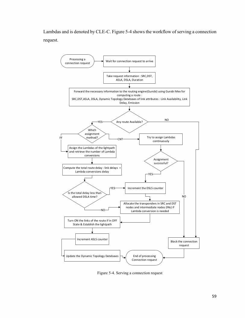
59
Lambdas and is denoted by CLE-C. Figure 5-4 shows the workflow of serving a connection
request.
Figure 5-4. Serving a connection request
Processing a connection request
Wait for connection request to arrive
Take request information : SRC,DST, ASLA, DSLA, Duration
Forward the necessary information to the routing engine(Gurobi) using Gurobi Mex for computing a route :
SRC,DST,ASLA, DSLA, Dynamic Topology Databases of link attributes : Link Availability, Link Delay, Emission
Update the Dynamic Topology Databases End of processing Connection request
Allocate the transponders in SRC and DST nodes and intermediate nodes (INs) if
Lambda conversion is needed
Turn ON the links of the route if in OFF State & Establish the lightpath
Compute the total route delay : link delays + Lambda conversions delay
Is the total delay less than allowed DSLA time?
Any route Available?
Block the connection request
Assign the Lambdas of the lightpath and retrieve the number of Lambda
conversions
Which assignment
method? Try to assign Lambdas continuously
Assignment successful?
CNT
YES
NO
FF
YESNO
Increment the DSLS counter YES
NO
Increment ASLS counter

60
After the route is computed, the route is given to the corresponding assignment method to
assign the Lambdas of the lightpath of the route. For CLE-C, the assignment is done with
the continuity constraint, and when it is successful, the Delay Satisfaction (DSLS) counters
are incremented as the route complies with the constraint of equation (5-6), and the
lightpath is established. As the next step, the ASLS counter is incremented. If any link of
the lightpath is in the OFF state, it is turned ON. Updating the dynamic topology
(accounting for the Lambdas that were assigned and marking them as occupied) concludes
the serving of the connection request with CLE-C. For CLE, the assignment method gives
the Lambdas of the route and the number of the Lambda conversions needed to establish
the lightpath. There is no chance of failure in the assignment with FF without the continuity
constraint as opposed to assignment with continuity constraint. This is because, if no
resources were available on the links, the route itself could not have been calculated using
the dynamic topology. After assigning the Lambdas for the lightpath, the total route delay
is calculated using Equation (2-3). If the total delay is less than the DSLA of the request,
the DSLA counter is incremented. To complete serving the request, “Lambda conversion
transponders” are assigned, and the lightpath is established. Notice that if the total delay is
higher than the DSLA value of the connection request, the route is still established but, the
Delay SLA satisfaction counter in not incremented. In this chapter no connection request
is blocked due to DSLA violation since other routing methods in the analysis section of
this chapter do not consider the DSLA at all. Not blocking the connection request due to
DSLA helps keeping the success rate of the CLE and CLE-C comparable to other
regenerated routing methods from Section 2.2.1 and 2.2.2. We will see that considering
DSLA in finding a route, increases the DSLA Satisfaction (DSLS) by about 15%. As the
last step of serving a connection request, the ASLA counter is incremented since the route
complies with the constraint of Equation (5-5). This ends the serving connection request
with CLE. Figure 5-5 shows the workflow of releasing a connection. When disconnecting
a lightpath, Lambdas of the route are released, and the transponders for adding and
dropping the Lambda as well as the transponders for Lambda conversion(s) are deallocated.
If a link is now accessible because it received back a resource from the lightpath, it is added
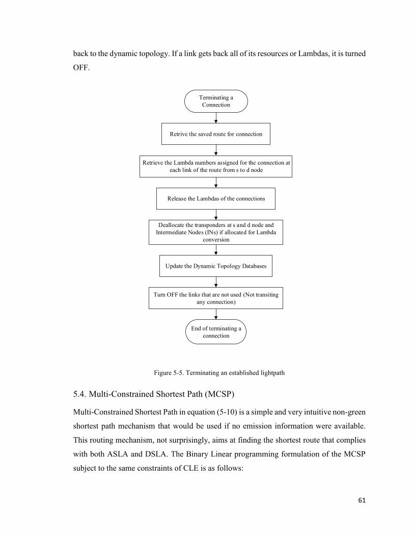
61
back to the dynamic topology. If a link gets back all of its resources or Lambdas, it is turned
OFF.
Figure 5-5. Terminating an established lightpath
5.4. Multi-Constrained Shortest Path (MCSP)
Multi-Constrained Shortest Path in equation (5-10) is a simple and very intuitive non-green
shortest path mechanism that would be used if no emission information were available.
This routing mechanism, not surprisingly, aims at finding the shortest route that complies
with both ASLA and DSLA. The Binary Linear programming formulation of the MCSP
subject to the same constraints of CLE is as follows:
Terminating a
Connection
Retrive the saved route for connection
Retrieve the Lambda numbers assigned for the connection at
each link of the route from s to d node
Release the Lambdas of the connections
Deallocate the transponders at s and d node and
Intermediate Nodes (INs) if allocated for Lambda
conversion
Update the Dynamic Topology Databases
Turn OFF the links that are not used (Not transiting
any connection)
End of terminating a
connection
62
𝑚𝑖𝑛 𝑧 = ∑ ∑ 𝐶𝑖𝑗 ∙ 𝑥𝑖𝑗
𝑗𝑖
(5-10)
In which Cij is the administrative or Link-State cost of each optical link. In this chapter by
considering Cij=1, MCSP performs the “Shortest Hop Count” operation.
CLE is compared against the EE, EASB, and MCSP with various performance metrics of
upcoming sections. CLE, CLE-C, and MCSP are constrained shortest path routing
methods. Therefore, their level of complexity is in order of O2.
The next section details the testbed information and the performance metrics for the
analysis of this chapter.
5.5. Analysis and Simulation Environment
5.5.1. The Network
The same network of Figure 1-1 is used in this chapter and each link has 96 numbered
Lambdas to assign without the continuity constraint, using First Fit (except for CLE-C), to
be consistent with regenerated routing mechanisms of EE and EASB. The availability of
optical links is randomly assigned a number from 0.9999 to 1 and is assumed to be constant
for the entire duration of simulations. Request for route or connection is simulated with a
Poisson process and is exponentially distributed with an arrival rate of 20 connections per
hour and mean duration of 10 hours. The ASLA for connection requests ranges from 0.999
to 0.99999, and DSLA is a multiple of 12.5 ms per time zone difference as illustrated in
Section 5.3.2. The optical links and elements of the forwarding plane may be placed in the
OFF state if they have no established lightpath. Each link and node is turned ON by a
mixture of green and non-green sources of energy resulting in overall energy dirtiness as
mentioned in Section 5.3.1.
5.5.2. Performance Metrics Used in This Chapter
Although some of these performance metrics have already been defined, they are revisited
here for sake of completeness.

63
ASLS
ASLS is the satisfaction rate of the ASLA. This metric is a ratio of the number of
connections that were served with a route that met their ASLA to the total number of the
served connections. CLE, CLE-C, MCSP and EASB that consider ASLA in finding a route
for a connection request, result in 100% ASLA satisfaction.
DSLS
DSLS is the satisfaction rate of the DSLA. This metric is a ratio of the number of
connections that were served with a route that met their DSLA, to the total number of the
served connections. CLE, CLE-C, and MCSP that consider DSLA in finding a route for
the connection request are expected to have higher satisfaction compared to other routing
mechanisms. Unlike ASLS, DSLS may or may not be 100% since the route which is not
complying with DSLA is not blocked.
Success Rate
The success rate is a ratio of the number of served requests over the total number of
requests.
Success Satisfaction
Success Satisfaction is the product of Success Rate, ASLS, and DSLS of a routing method.
This metric helps to analyse the overall satisfaction rate. Routing mechanisms such as CLE,
CLE-C, and MCSP that consider ASLA and DSLA in finding a route are expected to have
higher Success Satisfaction.
Lambda per Connection
This metric is the average length of the lightpath of the served connections in units of hops.
A lower number is preferred for this metric. A lower number indicates better resource
efficiency. Since the Traffic Engineering in GMPLS is in bidirectional fashion, the return
path is also considered in this graph. Therefore, the actual average length of the TE
lightpath in units of hops is the half of the number presented by this metric.
64
Emission per Lambda
This metric is the amount of emission emitted to the atmosphere to establish a unit resource,
Lambda. A lower number is preferred for this metric, and this metric shows the emission
reduction capability of a routing mechanism. The value of the emission per Lambda will
be lower for the routing mechanisms that have a higher success rate as the emission is
divided by more number of resources in operation. Because of this reason, emission
reduction must be evaluated and analysed for routing methods that have about the same
success rate.
Node Power
In this chapter, the node power is the power drawn by the optical forwarding layer of the
network. For each node, this power is the sum of energy used by transponders to add or
drop a Lambda as well as the energy used by transponders that perform the Lambda
conversion operation. Since adding and dropping a Lambda in a source node and a
destination node is the fixed part of the energy used by a node, the change in the value of
the energy usage for each node depends on the number of Lambda conversions. The value
of node power will be higher for the routing mechanisms that have higher success rate, and
therefore this metric must be evaluated for routing mechanisms that have the same success
rate.
Conversion Count
This metric is the total number of Lambda conversions in the network. In other words, the
sum of all Lambda conversions in every node of the network. With this metric, we can
observe the effect of using the combination of different routing and assignment methods.
Link Power
This metric is the power drawn by all turned ON links of the network. Since the power
drawn by the link does not change after being turned ON (since inline amplifiers and signal
leveling amplifiers amplify the entire spectrum or Lambdas), a lower value for this means
a lower number of links (inline amplifiers) are in operation.

65
The next section details the results of the analysis for CLE, CLE-C, MCSP, EASB and EE
using the introduced performance metrics.
5.6. Results
5.6.1. Graphical Presentation of the Obtained Results for Performance Metrics
As we can see in Figure 5-6, the success rate of EE is 100% since it does not consider any
SLA in serving a request and no blocking occurs due to SLA violation. 100% success rate
for this routing mechanism also means that there were enough resources to handle the given
traffic intensity and no connection request is blocked due to lack of resources. As we can
see in Figure 5-6, adding the delay constraint in finding a route reduces the success rate by
only 2% compared to EASB. In this figure CLE, CLE-C and MCSP are overlapping point
by point. With the same success rate for CLE, CLE-C, and MCSP and only 2% difference
compared to EASB, it is fair to compare these routing mechanisms against each other using
the remaining performance metrics. Figure 5-7, shows the ASLS percentage. As we can
see in this graph, without considering the ASLA in finding a route by EE, the ASLS drops
to 65% which may not be acceptable. As mentioned earlier the routing mechanisms that
serve the connection requests by considering the ASLA have a 100% ASLS which is the
case here for CLE, CLE-C, MCSP, and EASB. Figure 5-8, shows the results of analysis
for DSLS. As we can see in Figure 5-8, without considering the DSLA in finding a route,
DSLS can drop by more than 15% among routing methods that have about the same success
rate. As we can see in Figure 5-8, CLE is about 17% and 23% more DSLA compliant
compared to EASB and EE respectively. The non-green method of MCSP is about 2%
more DSLA compliant compared to CLE, because as we will see in later graphs, it has a
lower average hop length for the lightpaths. Therefore, MCSP has a lower chance of
Lambda conversion which may incur node delays. CLE-C is 100% DSLA compliant since
there is no Lambda conversion delay in the transit nodes of the lightpaths. Therefore, CLE
and CLE-C are better options compared to the hybrid green method of EASB and pure
green method of EE, regarding DSLA compliance. The results in Figure 5-9 for Lambda
per connection shows that the entire difference in resource efficiency of the green-aware
mechanism of CLE, CLE-C, EE and EASB is about 0.15 hops or 3%. Therefore, regarding
resource efficiency, these mechanisms are comparable and are about the same. Not
66
surprisingly, MCSP that aims at reducing the number of hops by performing constrained
shortest path has lower average Lambda per Connection and is about 10% or 0.4 hops more
resource efficient. In Figure 5-10 interesting results are obtained for link power that
represents the number of links in use. As we can see in this Figure, CLE, CLE-C, and EE
that performs constrained or direct shortest emission first routing, use fewer links and have
lower energy consumption in the links compared to EASB and MCSP. The reason is, CLE,
CLE-C and EE try to use most of the greener links and form a “Highway” across the
greener links, leaving the less green links in OFF state. On the other hand, MCSP performs
constrained shortest path, and EASB just chooses a route that has the lowest hybrid cost.
Therefore, they use more links. About 3 kW less power with the same SLA Satisfaction on
the network that has a total of 21 bidirectional links is desirable. Based on this graphs CLE
and CLE-C use less energy in the links compared to EASB and MCSP. Results of power
consumption of nodes in Figure 5-11 show that EE has the highest power consumption in
nodes. However, this is because EE has 100% success rate and establishes more
connections. Among CLE, MCSP and EASB that have about the same success rate and use
FF in Lambda assignment, MCSP uses about 4 kW less power because MCSP has lower
average route length as shown in Figure 5-9, and therefore, routes in MCSP transit less
number of nodes on an average. CLE-C with continuity constraint draws about 55% less
energy compared to MCSP because no Lambda conversion is performed in nodes as we
will see in the upcoming figure. With these observations, it is possible to conclude that
CLE-C is more energy efficient among other routing mechanisms compared in this Figure.
Figure 5-12 shows the results for the number of Lambda Conversion. As we can see in this
figure, CLE-C has zero number of Lambda conversions since it assigns the Lambdas with
a continuity constraint. MCSP, CLE, and EASB almost repeat the results of Figure 5-11,
and as we can see MCSP has a lower number of the Lambda conversions since again, the
average route length in MCSP is about 10% shorter and therefore less number of Lambda
conversions can happen. Therefore, CLE-C with the continuity constraint in the assignment
of Lambdas, and zero conversion, is more energy efficient than MCSP, EASB, CLE and
EE. The results for emission reduction in Figure 5-13 show that CLE is about 6% more
emission efficient than MCSP and about 3% more efficient than EASB. Not surprisingly
EE has a lower average because the total amount of emission is divided by more number

67
of established lightpaths and Lambdas as EE has 100% success rate. In this Figure, CLE-
C has about 37% less emission per unit resource Lambda compared to the non-green
MCSP, because as we saw, it a has a lower link and node power consumption and it chooses
the greener routes. The last graph in this section of analysis is the percentage of the Success
Satisfaction in Figure 5-14. As we can see in this Figure, although EE has 100% success
rate, because in has a poor ASLS and DSLS, it shows the lowest of the Success Satisfaction
percentage compared to other routing methods in this chapter. Among EASB, CLE, CLE-
C, and MCSP that have about 80% success rate CLE-C has the highest Success Satisfaction
rate as it has 100% ASLA satisfaction and 100% DSLA satisfaction. After CLE-C, MCSP
and CLE show about the same (1% difference) in success satisfaction since they have
acceptable DSLS and ASLS satisfaction. EASB although has 100% ASLS but because of
poor DSLS value, sits at 12% less Success Satisfaction compared to CLE.
Based on obtained results we can say that Constrained Shortest Path MCSP and
Constrained Least Emission CLE improve the DSLS by at least 15% compared to EASB,
using the constraint in Equation (5-6). The continuity constraint added to CLE (to come up
with CLE-C) provides the full 100% DSLS. Routing based on emission information
lowered the link energy usage and overall emissions. Routing based on shortest path
lowered the total node energy. However, the saving in energy and emission is much more
significant using continuity constraint. The difference of less than 10% in emission per unit
resource Lambda among CLE, EASB and MCSP is due to the fact that there is no 100%
pure green or non-green link. This result is in a big contrast to results of the paper in
[11,12,34,45,51] that use the concept of 100% green or 100% non-green energy for the
links.
In summary, the proposed CLE method with continuity constraint (CLE-C) has the best
emission reduction, highest Success Satisfaction rate, an acceptable resource usage, and
provides 100% Satisfaction for both ASLA and DSLA compared to other routing
mechanisms of this chapter. With continuity constraint and lower number of conversions
in CLE-C, a Service Provider can operate with a lower number of transponders used in
operation and have a more economical operation or lower Total Cost of Ownership (TCO).

68
This is added to the 55% less energy usage in nodes compared to the traditional non-green
routing mechanism of MCSP.
Figure 5-6. Success rate Figure 5-7. ASLS
Figure 5-8. DSLS Figure 5-9. Lambda per connection
Figure 5-10. Total link power Figure 5-11. Total node power

69
Figure 5-12. Total Lambda conversions Figure 5-13. Emission per Lambda
Figure 5-14. Success Satisfaction
5.6.2. Confidence Interval Analysis
Although the previous section provided a comprehensive analysis on the performance of
the CLE-C, this section is added to the study of the performance of CLE-C, to eliminate
any randomness. Since the availability of the links, availability of the green energy and
arrival of connection requests and their characteristics are random and simulated, the
simulation is repeated 100 times, processing 2 million connection request and building a
95% confidence interval over the mean of the average of some key performance metrics.
Based on results of Table 5-1, the success rate is about the same (1% difference) for EASB,
CLE, CLE-C and MCSP and their 95 % confidence interval has an overlapping section
which is desired.
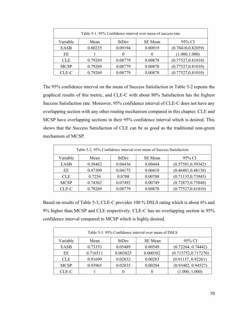
70
Table 5-1. 95% Confidence interval over mean of success rate
Variable Mean StDev SE Mean 95% CI
EASB 0.80235 0.09194 0.00919 (0.78410,0.82059)
EE 1 0 0 (1.000,1.000)
CLE 0.79269 0.08779 0.00878 (0.77527,0.81010)
MCSP 0.79269 0.08779 0.00878 (0.77527,0.81010)
CLE-C 0.79269 0.08779 0.00878 (0.77527,0.81010)
The 95% confidence interval on the mean of Success Satisfaction in Table 5-2 repeats the
graphical results of this metric, and CLE-C with about 80% Satisfaction has the highest
Success Satisfaction rate. Moreover, 95% confidence interval of CLE-C does not have any
overlapping section with any other routing mechanism compared in this chapter. CLE and
MCSP have overlapping sections in their 95% confidence interval which is desired. This
shows that the Success Satisfaction of CLE can be as good as the traditional non-green
mechanism of MCSP.
Table 5-2. 95% Confidence interval over mean of Success Satisfaction
Variable Mean StDev SE Mean 95% CI
EASB 0.58462 0.04436 0.00444 (0.57581,0.59342)
EE 0.47309 0.04175 0.00418 (0.46481,0.48138)
CLE 0.7254 0.0708 0.00708 (0.71135,0.73945)
MCSP 0.74362 0.07492 0.00749 (0.72875,0.75848)
CLE-C 0.79269 0.08779 0.00878 (0.77527,0.81010)
Based on results of Table 5-3, CLE-C provides 100 % DSLS rating which is about 6% and
9% higher than MCSP and CLE respectively. CLE-C has no overlapping section in 95%
confidence interval compared to MCSP which is highly desired.
Table 5-3. 95% Confidence interval over mean of DSLS
Variable Mean StDev SE Mean 95% CI
EASB 0.73353 0.05489 0.00549 (0.72264, 0.74442)
EE 0.716511 0.003825 0.000382 (0.715752,0.717270)
CLE 0.91699 0.02832 0.00283 (0.91137, 0.92261)
MCSP 0.93965 0.02835 0.00284 (0.93402, 0.94527)
CLE-C 1 0 0 (1.000, 1.000)
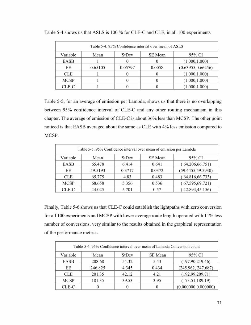
71
Table 5-4 shows us that ASLS is 100 % for CLE-C and CLE, in all 100 experiments
Table 5-4. 95% Confidence interval over mean of ASLS
Variable Mean StDev SE Mean 95% CI
EASB 1 0 0 (1.000,1.000)
EE 0.65105 0.05797 0.0058 (0.63955,0.66256)
CLE 1 0 0 (1.000,1.000)
MCSP 1 0 0 (1.000,1.000)
CLE-C 1 0 0 (1.000,1.000)
Table 5-5, for an average of emission per Lambda, shows us that there is no overlapping
between 95% confidence interval of CLE-C and any other routing mechanism in this
chapter. The average of emission of CLE-C is about 36% less than MCSP. The other point
noticed is that EASB averaged about the same as CLE with 4% less emission compared to
MCSP.
Table 5-5. 95% Confidence interval over mean of emission per Lambda
Variable Mean StDev SE Mean 95% CI
EASB 65.478 6.414 0.641 ( 64.206,66.751)
EE 59.5193 0.3717 0.0372 (59.4455,59.5930)
CLE 65.775 4.83 0.483 ( 64.816,66.733)
MCSP 68.658 5.356 0.536 ( 67.595,69.721)
CLE-C 44.025 5.701 0.57 ( 42.894,45.156)
Finally, Table 5-6 shows us that CLE-C could establish the lightpaths with zero conversion
for all 100 experiments and MCSP with lower average route length operated with 11% less
number of conversions, very similar to the results obtained in the graphical representation
of the performance metrics.
Table 5-6. 95% Confidence interval over mean of Lambda Conversion count
Variable Mean StDev SE Mean 95% CI
EASB 208.68 54.32 5.43 (197.90,219.46)
EE 246.825 4.345 0.434 (245.962, 247.687)
CLE 201.35 42.12 4.21 (192.99,209.71)
MCSP 181.35 39.53 3.95 (173.51,189.19)
CLE-C 0 0 0 (0.000000,0.000000)

72
This section confirmed the validity of graphical results obtained in the last section.
5.7. Summary and Future Work
This chapter introduced a multi-SLA aware routing mechanism that could provide 100%
DSLS and ASLS while operating at 55 % less node energy and 36% less emission
compared to tradition non-green mechanism. In this chapter, it was observed that
minimizing the emission of the route is as effective as (4 to 6) % in reducing the total
emission of the network when realistic emission values are used in the simulation and
analysis. The better and significantly more reduction of around 36% in emission emitted
by the network resulted by using continuity constraint that consumes 55% less energy. The
next chapter studies the performance of the continuity constraint on blocking rate of the
network.
73
Chapter 6 NHOPAKIND RESOURCE ASSIGNMENT METHOD
6.1. Introduction
The last chapter stated that continuity constraint might increase the blocking rate of the
network and it separated the routing step from the assignment step. This chapter introduces
a new energy efficient resource assignment method and compares it against FF and FF with
continuity constraint with five performance metrics. The introduced method aims at
reducing the energy usage at the forwarding layer of the nodes by reducing the number of
Lambda conversions. The assignment method introduced in this chapter can be an “add-
on” to any routing mechanism. For the analysis section of this chapter, The new assignment
method will be added to the process of serving a connection requests using Shortest Path
Routing mechanism. The testbed and the way that lightpaths are established are the same
as last chapter, except for the fact that each link is limited to have 16 available to assign
Lambdas to be able to simulate the congestion condition of the network easier. The
organization of this chapter is as follows: Section 6.1 introduces the new method. Section
6.2 provides a review of the performance metrics, details the test environment and explains
the traffic intensity scenarios. Section 6.3 elaborates the results with graphs and building
the Confidence Intervals. Section 6.4 provides the summary and states the future work.
Introduction to the assignment method comes next.
6.2. NHopAKind Resource Assignment
This section introduces the new proposed method for resource assignment called “N Hop
A Kind”, after a winning combination in the game of Poker. This method tries to find a
lightpath that has a zero or minimum Lambda conversion when no continuous lightpath to
the destination (assignment with continuity constraint) is available. When establishing a
lightpath with Lambda conversion, each group of Lambdas of the route are “N Hop A
Kind” before (each) conversion. The upcoming figures explain the process with an
example. In Figure 6-1, S is the source node, and D is the destination node. Each
Intermediate Node or (IN) is followed by a number that shows the place of the IN in the
route. Therefore, the first intermediate node in the path from S to D is IN1. The next hop
is IN2 in the route and so on. NHopAKind assignment method consists of two major steps.
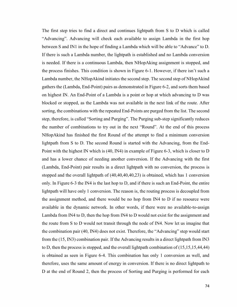
74
The first step tries to find a direct and continues lightpath from S to D which is called
“Advancing”. Advancing will check each available to assign Lambda in the first hop
between S and IN1 in the hope of finding a Lambda which will be able to “Advance” to D.
If there is such a Lambda number, the lightpath is established and no Lambda conversion
is needed. If there is a continuous Lambda, then NHopAking assignment is stopped, and
the process finishes. This condition is shown in Figure 6-1. However, if there isn’t such a
Lambda number, the NHopAkind initiates the second step. The second step of NHopAkind
gathers the (Lambda, End-Point) pairs as demonstrated in Figure 6-2, and sorts them based
on highest IN. An End-Point of a Lambda is a point or hop at which advancing to D was
blocked or stopped, as the Lambda was not available in the next link of the route. After
sorting, the combinations with the repeated End-Points are purged from the list. The second
step, therefore, is called “Sorting and Purging”. The Purging sub-step significantly reduces
the number of combinations to try out in the next “Round”. At the end of this process
NHopAkind has finished the first Round of the attempt to find a minimum conversion
lightpath from S to D. The second Round is started with the Advancing, from the End-
Point with the highest IN which is (40, IN4) in example of Figure 6-3, which is closer to D
and has a lower chance of needing another conversion. If the Advancing with the first
(Lambda, End-Point) pair results in a direct lightpath with no conversion, the process is
stopped and the overall lightpath of (40,40,40,40,23) is obtained, which has 1 conversion
only. In Figure 6-3 the IN4 is the last hop to D, and if there is such an End-Point, the entire
lightpath will have only 1 conversion. The reason is, the routing process is decoupled from
the assignment method, and there would be no hop from IN4 to D if no resource were
available in the dynamic network. In other words, if there were no available-to-assign
Lambda from IN4 to D, then the hop from IN4 to D would not exist for the assignment and
the route from S to D would not transit through the node of IN4. Now let us imagine that
the combination pair (40, IN4) does not exist. Therefore, the “Advancing” step would start
from the (15, IN3) combination pair. If the Advancing results in a direct lightpath from IN3
to D, then the process is stopped, and the overall lightpath combination of (15,15,15,44,44)
is obtained as seen in Figure 6-4. This combination has only 1 conversion as well, and
therefore, uses the same amount of energy in conversion. If there is no direct lightpath to
D at the end of Round 2, then the process of Sorting and Purging is performed for each

75
End-Point of Round 2 and the NHopAkind method enters the Round 3. In Round 3 at each
End-Point of Round 2, the highest (or the nearest to D) End-Point or IN is selected for
Advancing to D and finding a direct lightpath. Advancing continues to find a direct
lightpath as we will see in Figure 6-5. To explain the process in Round 3 and later Rounds,
let us number each End-Point. For example, Lambda 20 from S is stopped at IN3 and gets
R1E1 denoting Round 1 End-Point 1. R2E3, therefore, is the 3rd End-Point in Round 2. As
we can see in Figure 6-5, Advancing is started from End-Points of the last Round to find a
continuous lightpath. When a continuous lightpath is found, the Lambda numbers of the
entire route can be found by “Reversing” to S by knowing the “Parent” of the End-Point
that resulted in the continuous lightpath. For example, in Figure 6-5 Lambda number 3
with End-Point of R3E2 reached to D and to find the Lambdas for the entire route we need
to “Reverse” back to S. The Parent of the End-Point R3E2 is R2E2, whose parent is R1E1.
By knowing the Parents of the Endpoints Lambdas of the path can “Compiled”, as we can
see in Figure 6-5. As soon as finding a direct lightpath in Round 3 or any Round, in general,
the process is stopped, and there is no need to check the other combinations. This
significantly improves the resolution time of NHopAkind method. It can be concluded that
at the end of each round R, a lightpath with R-1 conversions may be found. The network
testbed in this chapter has an average route length of around 2.5 hops (as we will see in the
results section). Therefore, NHopAkind may do up to 3 Rounds on an average.
Figure 6-1. Advancing step Figure 6-2. Sorting and Purging step

76
Figure 6-3. 1 conversion in last IN Figure 6-4. Equivalent alternate lightpath with 1
conversion
Fot this chapter SP routing method is paired with the First Fit, First Fit with continuity
constraint and the NHopAkind and calls the combinations SP, SPCont and SPNHK
respectively.
Figure 6-5. Advancing step in Round 3
Table 6-1. shows the algorithm of the NHopAking in form of pseudocode.
Table 6-1. NHopAkind Algorithm
INPUT : Route; Lambda : Resource matrix; LAM_NUM : Max available Lambda per link;
Flag : Resource availability flag;
OUTPUT : RET_Flag: Updated resource availability flag;
RT : Route Lambdas; Connum : Number of Lambda conversions;
Function [RET_Flag,RT,Connum] =AssignNHopAkind(Route,Lambda,LAM_NUM,Flag)
MAX_COL=2;SORT_COL=2; NODENUM=14; RTlambda=[]; %the lambda assignment to return
R_len=length(Route)-1;
Continuous=0; End_Point2_NUM(1:NODENUM)=0;
offset=1; %the reference point for howmany hops to go to get blocked

77
Initialize(End_Points,0)
End_Point=[];
[l,Continuous,Flag,End]= Advance(Lambda,Route,Flag,End,LAM_NUM);
%this is the location of Lambdas crossed or stopped and need conversion if Continuous
RT(1:r_len)=l;
Connum=0; else
End_Point=Sort(End,Route,LAM_NUM,MAX_COL,SORT_COL,Lambda);
End_point2=purgeRepeatedEnd(End_Point); End_point2_set{1,1}=End_point2;
End_Point2_NUM(1)=1;
i=1;Round=2; while i<NODENUM && ~Continuous
s=1;j=1;
while (j<=End_Point2_NUM(Round-1) && ~Continuous) End_Point2_NUM(Round-1);
pretempcrosspoint2=End_point2_set{Round-1,j};
Sizepretemp=size(pretempcrosspoint2);
k=1;
while (k<=Sizepretemp(1) && ~Continuous)
temproute=Route(pretempcrosspoint2(k,2):length(Route)); offset=pretempcrosspoint2(k,2);
[l,Continuous,Flag,End]= Advance(Lambda,temproute,Flag,End,LAM_NUM);
End_Point=[]; if ~Continuous
End_Point=cross2point(End,temproute,LAM_NUM,MAX_COL, SORT_COL,Lambda);
End_point2=purgeRepeatedEnd(End_Point); cross_point3=addOfsetNode(End_point2,offset);
End_point2_set{Round,s}=cross_point3;
Crosspoint2_parent{Round,s}=[Round-1,j,k]; End_Point2_NUM(Round)=End_Point2_NUM(Round)+1; % number of cross points existing
end
s=s+1; k=k+1; end
j=j+1;
end
Round=Round+1; i=i+1;
end
RTlambda=[RTlambda,ones(1,length(pretempcrosspoint2(k-1,2):length(Route)))*l]; tempC=[];tempC(1)= Round-2 ;tempC(2)= j-1; tempC(3)=k-1; Finalpoints=[];
%Since with lower rounds Crosspoint2_parent is not defined then we will
%make a dummy one here so loop does not break if (Round<=3)
Crosspoint2_parent{tempC(1),tempC(2)}=[];
end while (Round-2)>=1
temp=End_point2_set{tempC(1),tempC(2)}(tempC(3),:);
Finalpoints=[Finalpoints;temp]; tempC=Crosspoint2_parent{tempC(1),tempC(2)};
Round=Round-1; end
RT=[];
Finalpointslen=size(Finalpoints); Startnode=1;
if Finalpointslen(1)>1
Finalpoints=flip(Finalpoints); end
start=1; temp=[];
for i=1:Finalpointslen(1) temp(start:Finalpoints(i,2)-1)=Finalpoints(i,1);
start=Finalpoints(i,2);
end RT=[temp,RTlambda(1:length(RTlambda)-1)];
Connum=Finalpointslen(1)+1;
End for k=1:( R_len)
RET_flag=UpdateFlag(Route,Flag,Lambda)
end end

78
Figure 6-6 demonstrate the process of serving a connection request which is similar to the
workflow of the last chapter. When a connection request arrives, first a route using SP
method is computed. With SPCont the assignment process attempts to assign the resource
of Route continuously, and if it succeeds, the lightpath is established in the next upcoming
step. If the assignment is not successful, the connection request is blocked. With SP and
SPNHK the resources of the route are assigned by corresponding assignment methods
which give the Lambdas of the route and the number and place (INs) of the Lambda
conversions. Regardless of the assignment method, after assigning the resource, the
dynamic topology table is updated, and if a link is in the OFF state, it is turned ON. If a
link just assigned its last resource and can not take any more lightpaths, it is removed from
the dynamic topology, so no new route is computed using that link. As the last step the
transponders of S, D, and INs (if Lambda conversion is needed) are allocated, and the
lightpath is established. This concludes the serving a connection request. The process of
releasing a lightpath is the same as in the last chapter and is not repeated here.
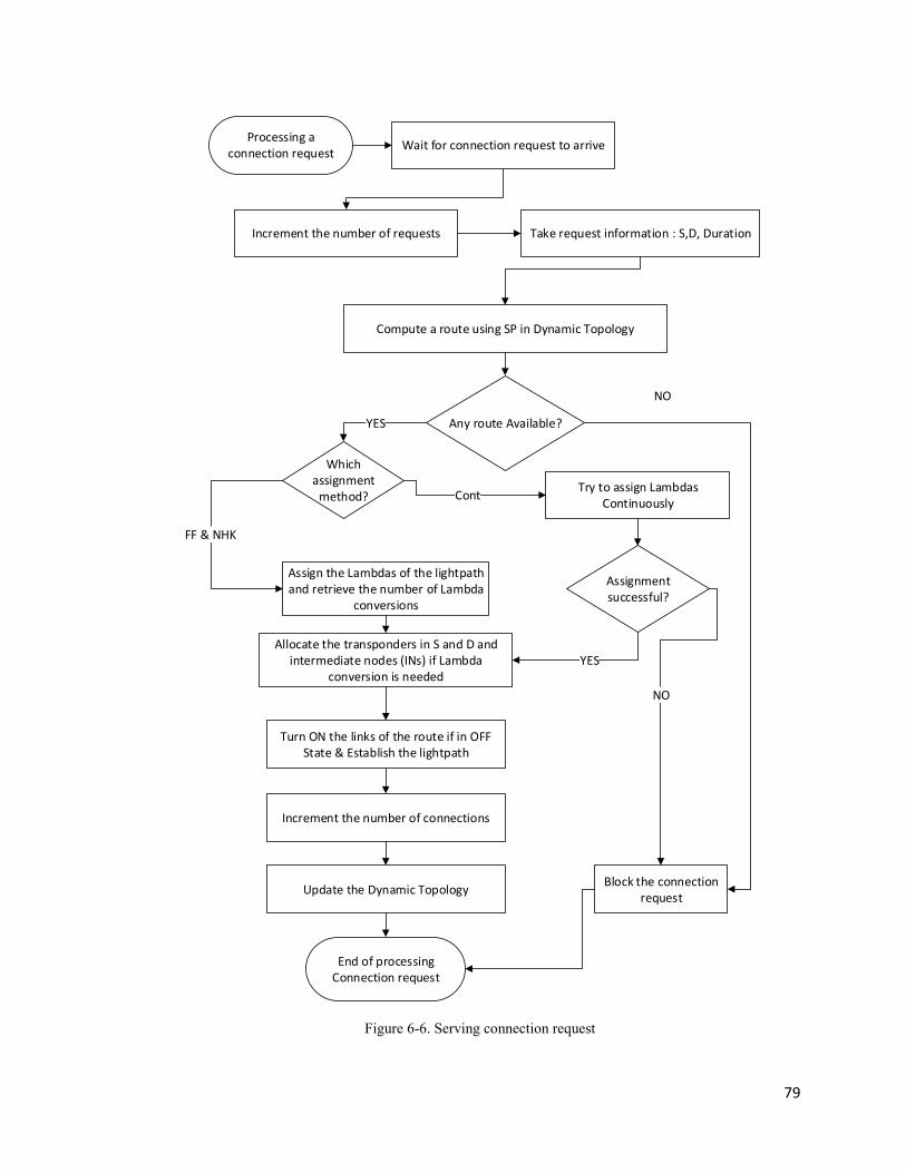
79
Processing a connection request
Wait for connection request to arrive
Take request information : S,D, Duration
Compute a route using SP in Dynamic Topology
Update the Dynamic Topology
End of processing Connection request
Allocate the transponders in S and D and intermediate nodes (INs) if Lambda
conversion is needed
Turn ON the links of the route if in OFF State & Establish the lightpath
Any route Available?
Block the connection request
Assign the Lambdas of the lightpath and retrieve the number of Lambda
conversions
Which assignment
method?Try to assign Lambdas
Continuously
Assignment successful?
Cont
YES
NO
FF & NHK
YES
NO
Increment the number of requests
Increment the number of connections
Figure 6-6. Serving connection request
80
6.3. Analysis
6.3.1. Testbed Network
The network of the last chapter is used in this chapter with the same optical elements. The
behaviour of the traffic is simulated with a Poisson process with an arrival rate of 20, 80
and 125 connection requests per hour, for scenario 1 scenario 2 and scenario 3,
respectively. The duration of the connections or lightpaths also follows an exponential
distribution with a mean duration of 30 mins. Each link has 16 available to assign Lambdas.
The simulation to obtain the results of each routing and assignment pair is performed in
parallel and independently using MATLAB Parallel Toolbox [18]. Introduction to the
performance metrics used in this comes next.
6.3.2. Performance Metrics
Number of Conversions
This metric simply shows the total number of current Lambda conversions at each time of
the day. Depending on the traffic scenario and the assignment method used, this number
can be different for each routing-assignment pair. Obviously, a lower value is preferred for
this metric. It is expected that continuous and NHopAkind methods have zero Lambda
conversion in scenario 1, since there are enough resources to establish the lightpaths
“continuously.”
Lambda per Edge
This metric is the average number of the connections per each link of the network. This
metric shows how congested the network links are on an average.
6.4. Results
6.4.1. Analysis for Scenario 1: The Light Traffic
As we can see in Figure 6-7, The success rate of the network for all routing mechanism of
SP, SPCont and SPNHK is the same. The reason is that there are enough resources to
establish the lightpaths regardless of assignment mechanism used. As we can see in Figure
6-8, the average utilization of the links of the network is 2.5 out of 16 available-to-assign
Lambdas and the network is not congested at all with the light traffic of scenario 1. As we

81
can see in Figure 6-9, since there is no congestion on the links due to the light traffic, SP,
SPNHK and SPCont give the same route length on an average. Figure 6-10, for this
scenario, shows that the Continuous and NhopAkind become the same, as NHopAkind
assigns the resources with minimum Lambda conversion, which is zero for this scenario.
This fact is shown with overlapping SPCont and SPNHK in Figure 6-10. SP with FF in this
case assigns the resources of the lightpaths with a total of 16 Lambda conversions. With a
lower number of conversions, the total node energy is about 50% less for SPNHK and
SPCont compared to SP as we can see in Figure 6-11. The results of analysis for scenario
1 concludes that continuous assignment and NHopAkind assignment are the same when
the traffic intensity and utilization of the links are low. The same analysis is performed for
scenario 2 and 3.
Figure 6-7. Success rate Figure 6-8. Lambda per edge
Figure 6-9. Lambda per connection Figure 6-10. Lambda conversions count

82
Figure 6-11. Total node power
6.4.2. Analysis for Scenario 2: The Moderate to Heavy Traffic
As we can see in Figure 6-12, the success rate of SPCont drops by 6%. SPNHK and SP
still provide almost 100% success rate and are overlapping in this figure. Therefore, the
6% drop in the success rate of SPCont is due to lack of continuous lightpaths and not lack
of available resources. Results of Figure 6-13, shows that the average congestion of the
links of the network is around 50% of the 16 available to assign Lambdas per each link or
edge. In Figure 6-13 SPNHK and SP have higher link utilization, first, because they have
a higher success rate, and because they assign the resources to the routes that bypass the
congested links and are longer on an average. The fact that the routes assigned by SP and
SPNHK are longer than SPCont is clearly shown in Figure 6-14. As we can see in Figure
6-14, the overlapping value of average route length for SP and SPNHK is about 8% higher
compared to SPCont. Therefore, routes are 8% longer on an average trying to establish the
lightpath through the links that still have the resources (Lambdas to assign). With the
results of Figure 6-15 for Lambda conversion count, we can see that SPNHK is minimizing
the Lambda conversion by 72%. Therefore, SPNHK performs 72% less Lambda
conversions and gives the same route length to provide 100% success rate compared to SP.
SPCont (not surprisingly) gives zero Lambda conversion count. The lower Lambda
conversion number with SPNHK compared to SP is also reflected in results of Figure 6-16
for node power consumption, and SPNHK consumes about 44% % less energy compared
to SP.

83
Figure 6-12. Success rate Figure 6-13. Lambda per edge
Figure 6-14. Lambda per connection Figure 6-15. Lambda conversion count
Figure 6-16. Node power

84
6.4.3. Analysis for Scenario 3: Heavy Traffic
As we can see in Figure 6-17, the success rate of the network drops quite a bit by about
20%. However, the overlapping success rate of SP and SPNHK is about 3% higher
compared to the SPCont. SPNHK and SP try to use any possible route and resource to
establish the lightpath. The level of congestion in Figure 6-18, shows that the network is
almost completely congested as the average of 13 out of 16 available to assign Lambdas of
the links are already established and taken. As mentioned earlier this situation happens
when SP and SPNHK assign the resources for the routes that are longer on an average
trying to bypass the congested links and establish the lightpath. As we can see in Figure
6-19, SP and SPNHK chose any remaining route and available resources to establish the
lightpaths and therefore, the average route length is about 38% longer compared to SPCont.
By increasing the route length, the probability of having more Lambda conversion is
increased and therefore SPNHK behaves almost the same as SP with only 14% less
conversion as we can see in Figure 6-20. However, SPNHK consumes about 26% less
energy to give the same success rate of SP which is about 2.5% to 3% higher than SPCont
as shown in Figure 6-21. Depending on the value of the connections requests, 3% more
success rate may or may not be reasonable to spend 38% more resources and 47% more
energy compared to SPCont. However, since the assignment process is separated from the
routing process, depending on the congestion condition of the network different assignment
mechanisms can be used that are more energy and resource efficient than FF. We can
conclude that it is reasonable to use NHopAking when the traffic intensity of the network
is low to moderately high, to gain more success rate and save energy. However, it may be
reasonable to switch to the continuous assignment of resources when traffic intensity is
higher, and the network is congested. The average number of assigned Lambdas for a link
is a good indication of the congestion level of the network.
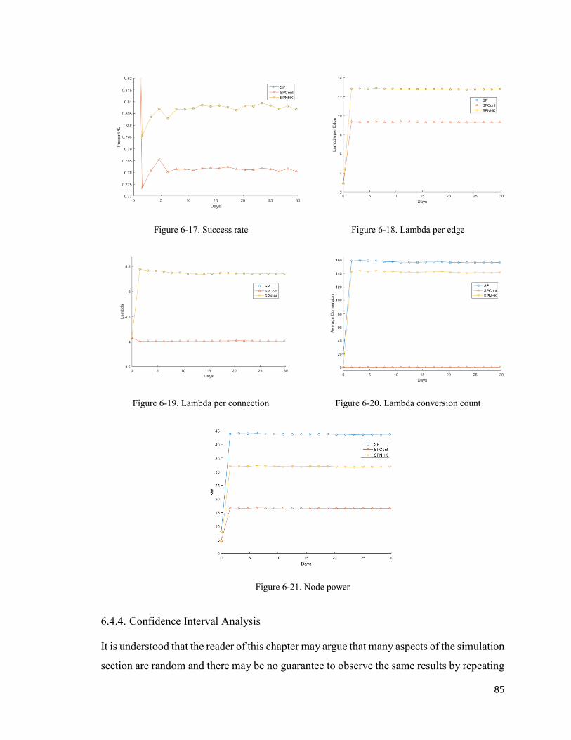
85
Figure 6-17. Success rate Figure 6-18. Lambda per edge
Figure 6-19. Lambda per connection Figure 6-20. Lambda conversion count
Figure 6-21. Node power
6.4.4. Confidence Interval Analysis
It is understood that the reader of this chapter may argue that many aspects of the simulation
section are random and there may be no guarantee to observe the same results by repeating

86
the simulation. Therefore, this text-based section presents the analysis on Confidence
Intervals (CIs) of the performance metric. Using Minitab in [21], the mean and the 95% CI
over the average of the mean is computed for four important performance metrics with 70
independent and parallel runs of the simulation, equivalent to processing and analyzing 5.6
million connection requests. The traffic intensity chosen for this analysis is the arrival rate
of 100 connections per hour with the same 30-minute average duration. 100 connections
per hour was chosen to push the network to even more congestion level of scenario 2 but
avoiding almost the complete congestion of scenario 3 with more than 20% drop in success
rate. The analysis for an average of mean success rate in Table 6-2 shows about 8% more
success rate for SPNHK compared to SPCont in the “busy time”. It is also important to
notice that the 95% CIs of SPNHK and SPCont do not overlap at all which means SPNHK
will have a higher success rate at 100 connections per hour. The analysis for route length
average in Table 6-3 shows that SPNHK will increase the length of the routes on an average
to use all available resources and ensure higher success rate of the network. The CI of the
SPNHK for average route length confirms that resources of longer routes will be assigned.
The results of CI analysis for node power in Table 6-4 shows that SPNNHK is about 35%
more energy efficient compared to SP. There is no overlapping between CIs of the SP and
SPNHK. Finally, for the number of Lambda Conversion in Table 6-5, we can see that
SPNHK has about 33% less number of conversions compared to SP. The CIs of SPNHK
and SP do not overlap.

87
Table 6-2. 95% Confidence interval over mean of success rate
Variable Mean StDev SE Mean 95% CI
SP 0.938834 0.002763 0.00033 (0.938175, 0.939492)
SPCont 0.864415 0.002121 0.000254 (0.863909, 0.864921)
SPNHK 0.938834 0.002763 0.00033 (0.938175, 0.939492)
Table 6-3. 95% Confidence interval over mean of route length
Variable Mean StDev Mean 95% CI
SP 4.98931 0.02615 0.00313 (4.98308, 4.99554)
SPCont 4.13763 0.00996 0.00119 (4.13526, 4.14001)
SPNHK 4.98931 0.02615 0.00313 (4.98308, 4.99554)
Table 6-4. 95% Confidence interval over mean of node power (kW)
Variable Mean StDev Mean 95% CI
SP 37.6009 0.2301 0.0275 (37.5460, 37.6557)
SPCont 14.533 0.0527 0.0063 (14.5205, 14.5456)
SPNHK 24.2334 0.2444 0.0292 (24.1751, 24.2917)
Table 6-5. 95% Confidence interval over mean of number of Lambda conversions
Variable Mean StDev Mean 95% CI
SP 128.494 1.186 0.142 (128.211,128.776)
SPCont 0 0 0 (0.000000, 0.000000)
SPNHK 86.678 2.067 0.247 (86.185, 87.171)
6.5. Summary and Future Work
Based on results obtained in this chapter, it can be concluded that NHopAking is as good
as a Continuous method regarding the success rate and resource utilization when traffic
intensity is light. With higher traffic intensity NHopAking uses more resources to keep the
success rate higher, compared to the continuous method. Although NHopAkind is using
longer routes to establish the lightpaths, it uses (35-50)% less energy to give the same
success rate of the First Fit method. In any case, the number of Lambda conversions
performed by NHopAkind is lower than the First Fit for the same success rate. In the busy
times of the network, NHopAKind gives up to 8% more success rate compared to the
continuous method which can be considered as 8% more income for the service provider.

88
NHopAkind method will be tested with different average durations of the lightpaths and a
higher number of the available resources per link, in future.
"MINITAB® and all other trademarks and logos for the Company's products and services are the exclusive property of Minitab Inc.
All other marks referenced remain the property of their respective owners. See minitab.com for more information."

89
Chapter 7 SUMMARY AND FUTURE WORK
This chapter summarizes the contributions of this thesis. With the stateless routing
mechanisms of Chapter 3, the throughput of the control plane of the GMPLS network can
be increased by 6-fold when compared to traditional routing mechanisms that perform the
routing operation on arrival of the connection request. The FL-EASB introduced in Chapter
3 can use the futuristic information to handle the maintenance windows (Not using a link
in maintenance window). Furthermore, T-EASB and FL-EASB are examples of the routing
mechanisms to be used with a stateless mechanism. Any other routing such as the routing
mechanism introduced in Chapter 5 can be used to populate the routing table on the fly or
use the predicted information. As the resource assignment is done separately, any resource
assignment such as the one introduced in Chapter 6 can perform the resource assignment
with the stateless approach. As future work, the success rate of T-EASB and FL-EASB
will be tested with the newly proposed resource assignment of Chapter 6. The Table Driven
Constrained Least Emission T-CLE routing mechanism will also be developed to improve
the throughput of the control plane that is using CLE-C mechanism.
Chapter 4 showed the importance of developing effective green routing mechanisms as
they perform better than traditional routing mechanisms that adopt the GSLA for reducing
the emission of the network. Chapter 4 also showed that by adopting GSLA by traditional
non-green mechanism would not give the accepted resource efficiency and will have
increased resource utilization, again, in return for an unacceptable reduction in emission.
It was shown that by as low as 20% increase in the amount of available green energy in the
network connection requests with much higher GSLA requests of up to 80% can be
accommodated with 90% success rate. The effect of adding Green SLA (using the realistic
energy and emission information of Chapter 5) on the behavior of key performance metrics
of the optical network will be evaluated.
Chapter 5 introduced a Multi-SLA aware routing mechanism which is more practical to be
implemented in the control plane of the GMPLS network. The CLE and EE outing
mechanism form a highway over greener links. CLE-C provides 100% Satisfaction for
ASLA and DSLA and emits the least emissions compared to other routing mechanisms.
By analyzing the outcome of simulation for 2 million connection requests and performing

90
the CI analysis it can be confirmed that the obtained results are acceptable. Chapter 5 also
computed the realistic information for the testbed. Table A-1 is the result of gathering more
that 50,000 records and it is expected that this energy table will be used by other papers
that need the set of realistic information for energy and emission in any networking field.
The results of Chapter 5 have been obtained by interfacing MATLAB with a state of the
art optimization solver, Gurobi. For connecting these two softwares, Chapter 5 used a
newly developed code in MATLAB that is going to be shared in “MATLAB Central” for
public use. Future work will add a set of new device and energy specific constraints to the
formulation of CLE to make it even more practical and usable. For example, the constraint
of the maximum energy draw possible per node will be added. The performance of CLE
with NHopAkind resource assignment method for the higher intensity of the traffic will
also be evaluated.
Chapter 6 developed and tested a new assignment mechanism that can increase the success
rate of the network when traffic intensity is higher than normal. The NHopAKind resource
assignment provided up to 8% more success rate compared to FF with continuity constraint
while using 37% less energy compared to FF that provides the same success rate. Chapter
6 suggested switching between resource assignment mechanisms depending on the
congestion level of the network. Similar to Chapter 5 for performing the CI analysis
Chapter 6 combined and used the data resulting from processing 5.6 Million connection
requests. With this analysis, it was confirmed that results obtained for the performance of
NHopAKind are comparable or better than FF with the continuity constraint. The success
rate of the network when pairing NHopAkind with different routing mechanisms will be
studied in future work.
The routing and assignment mechanism provided in the thesis can be used with any Link-
State environment and can be ported to other controller based systems such as SDN
controllers.

91
Appendix A. Total Generation Capacity in the US in 2011
Numbers in units of MW.
Table A-1. Total generation capacity in the US in 2011
States\Source Pumed Wind Hydro Solar Nuclear Geo Thermal Coal Natural Gas Other Gas Bio Mass Wood petroleum
AK 0 0 0 0 0 7.4 413.95 0 0 881.25 698.95 110.95
AL 0 0 0 593.15 0 0 3221.8 5089.25 82.8 12609.55 45.05 11478.65
AR 28 21.1 0 311.2 0 0 1336.2 1844 0 8038 22 4535
AZ 216.3 6.8 0 28 128.55 138.1 2720.4 3937 0 14017.55 100.7 6227.5
CA 3839.45 407.15 2055.95 640.5 589.25 3768.4 10123.95 4390 212.6 41775.9 527.45 411.7
CO 562.5 13.6 0 0 85.5 1792.9 657 0 0 5510.1 188.5 5605.2
CT 29.2 174.6 0 0 0 0 123.6 2109.5 0 3083 3278.55 566.45
DC 0 0 0 0 0 0 0 0 0 10 790 0
DE 0 8 0 0 12.5 2 0 0 135 2286 116.8 794
FL 0 666.85 0 359 64.6 0 54.5 3970.5 0 34962.8 10970.75 10253.5
GA 1861.5 24.2 0 623.9 0 0 2046.25 4061 0 15009.45 1390.1 13007.75
HI 0 222.25 31 0 2.2 91.6 23.55 0 12.2 0 2001.4 180
IA 0 14.6 0 0 0 4206.55 141.5 611.75 0 2501.05 1071.1 6947.9
ID 0 12.3 11.1 75.8 0 611.3 2654.2 0 0 879.25 5.4 17.2
IL 0 127.8 0 0 9 2737.3 34.1 11560.5 117.7 14562.8 943.4 14956.05
IN 0 53.75 0 0 0 1339.7 60.1 0 535.3 5993.85 472.05 19013.4
KS 0 7.1 0 0 0 1271.8 2.65 1190 0 4661.2 550.9 5188.2
KY 0 16.8 0 57.85 0 0 792.9 0 0 5327.85 73.4 15395.85
LA 0 13.9 0 311.35 0 0 192 2145 33.3 19390.65 997.9 3419
MA 1680 270.85 0 25.7 11.3 29.65 263.25 684.7 0 6430.65 3230.6 1579.55
MD 0 137.9 0 2.1 4.4 120 590 1719.5 152.35 2106.95 2998.45 4890
ME 0 91.15 0 609.85 0 322.5 743.8 0 0 1725.2 1016.1 90
MI 1851.3 184.55 0 263.8 0 374.6 235.35 4044.1 0 11687.15 707.3 11514.15
MN 0 210.9 0 162.15 0 2576.6 197.45 1633.5 0 5188.25 852.3 4713.1
MO 667 7.7 0 0 0 458.5 567.65 1215 0 5811.3 1316.7 12486.1
MS 0 0 0 228.6 0 0 0 1195.5 4 11979.55 37.5 2546
MT 0 0 0 0 0 378.2 2742.3 0 1.5 390.5 55.5 2442.3
NC 76.75 43.1 0 480 39.1 0 1956.9 5073 0 8492.95 596 12370.95
ND 0 9.8 0 0 0 1422.9 508 0 8.4 10.1 72.05 4151.3
NE 0 10.9 0 0 0 332.5 278.2 1244.5 0 1776.3 363.2 4108.3
NH 0 29.8 0 128.85 0 24 495.2 1246.45 0 1284.9 508.9 549.95
NJ 400 213.75 0 0 145.65 7.5 5.25 4192.6 0 10618.15 1472.75 1992.85
NM 0 6.5 0 0 129.5 750.2 82.9 0 0 3365.55 4.4 3990
NV 0 0 358.8 0 125 0 1051 0 0 7511.7 11.4 2873.8
NY 1400 363.9 0 86.1 31.5 1398.9 4334.95 5253.75 0 19618.1 5390.5 2815.55
OH 0 58.3 0 63.65 22.4 159.7 104.65 2155 116.2 8747.55 1095.15 21300.4
OK 260 15.7 0 57.8 0 1810.8 858.2 0 0 13607.8 69.3 5312
OR 0 35.9 0 243.35 2.6 2208 8426.35 0 0 3151.65 0 585
PA 1521 433 0 107.2 17.95 789.3 772.6 9784 105.2 10308.05 4473.7 18181.1
RI 0 23.7 0 0 0 1.5 2.7 0 0 1836.8 17.4 0
SC 2716 33.7 0 257 0 0 1337.6 6572.5 0 5698.85 736.5 7284.25
SD 0 0 0 0 0 780 1594 0 0 730.6 247.25 496.6
TN 1616.3 6.8 0 185.25 0 29.1 2525.75 3456.1 0 5042.5 39.6 8657.1
TX 0 127.2 0 215.15 43.5 10361.75 689.3 4990 310.9 70802.35 208.85 23258.4
UT 0 9 45.5 0 0 324.4 251.8 0 0 2061.35 27.8 4903
VA 3241 295.1 0 363.65 0 0 892.05 3596.5 0 8666.05 2448.65 5905.95
VT 0 3.2 0 76.75 2.2 45.1 324.65 624.15 0 0 116.55 0
WA 314 64.6 0 319.7 0.5 2453.5 20969.9 1117.5 0 4026.1 15.2 1340
WI 0 88.1 0 236.1 0 615.45 383.95 1756 0 6416.9 800.7 8440.1
WV 0 2.2 0 0 0 528.1 289.2 0 0 1098.9 13 15527.1
WY 0 0 0 0 0 1412.4 305.65 0 99.15 130.7 5.8 6499.4

92
Appendix B. Licenses
Figure B-1. License to use EASB flowchart
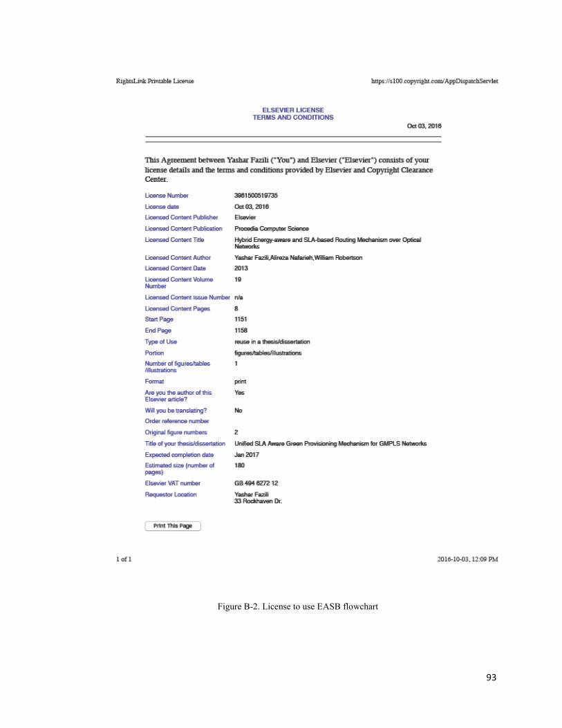
93
Figure B-2. License to use EASB flowchart

94
Figure B-3. License to use A-EASB flowchart

95
Figure B-4. License to use NSFnet diagram
96
Figure B-5. License to use T-EASB time performance graphs

97
Figure B-6. License to use full text of Chapter 4
98
Figure B-7. License to use Figure 1 of EASB paper in [13]

99
REFERENCES
[1] Renzenbrink T. How Much Electricity Does the Internet Use? 2013; Available at:
http://www.techthefuture.com/technology/how-much-electricity-does-the-internet-use/, Accessed,
2015.
[2] Strickland J. How much energy does the Internet use?. 2012; Available at:
http://computer.howstuffworks.com/internet/basics/how-much-energy-does-internet-use2.htm.
Accessed September, 8, 2016.
[3] T. J. Blasing. 2015, Investigation Report, 10.3334/CDIAC/atg.032.
[4] CBC. U.S., China agree to cut greenhouse gases in bid to spur others to join. 2014; Available
at: http://www.cbc.ca/news/politics/u-s-china-agree-to-cut-greenhouse-gases-in-bid-to-spur-
others-to-join-1.2832053;. Accessed Feb 3, 2015.
[5] McCarthy S. Trudeau, Obama and Pena Nieto agree to emission-reduction goals at summit.
2016; Available at: http://www.theglobeandmail.com/report-on-business/industry-news/energy-
and-resources/three-amigos-agree-to-clean-energy-partnership/article30674952/. Accessed
Oct/23, 2016.
[6] Chris Mooney SM. In a major moment for climate policy, China, Brazil, and the U.S. all
announce new commitments. 2015; Available at: https://www.washingtonpost.com/news/energy-
environment/wp/2015/06/30/china-brazil-and-the-u-s-all-announce-new-climate-and-clean-
energy-goals/;. Accessed Jun 30, 2015.
[7] EPA. Cap and Trade. 2012; Available at: http://www3.epa.gov/captrade/. Accessed May 10,
2015.
[8] Ontario G. Cap and Trade. October, 2016; Available at: https://www.ontario.ca/page/cap-
and-trade. Accessed October, 2016, 2016.
[9] Kanter J. Europe Considers New Taxes to Promote 'Clean' Energy. 2010; Available at:
http://www.nytimes.com/2010/06/23/business/energy-
environment/23carbon.html?_r=5&ref=cap_and_trade&. Accessed Jan 15, 2015.
[10] Thomas Bruckner and et. all. 2014; Mitigation of Climate Change, Annex III: Technology -
specific cost and performance parameters. Available at: http://www.ipcc.ch/pdf/assessment-
report/ar5/wg3/ipcc_wg3_ar5_annex-iii.pdf.
[11] Jiayuan Wang, S. Ricciardi, A. M. Fagertun, S. Ruepp, D. Careglio and L. Dittmann.
Energy-aware routing optimization in dynamic GMPLS controlled optical networks. Transparent
Optical Networks (ICTON), 2012 14th International Conference on; 2012.
[12] Ricciardi S, Wang J, Palmieri F, Careglio D, Dittman L. An energy-aware engineered
control plane for wavelength-routed networks. Transactions on Emerging Telecommunications
Technologies 2015;26(2):231-249.
[13] Fazili Y, Nafarieh A, Robertson W. Hybrid Energy-aware and SLA-based Routing
Mechanism over Optical Networks. Procedia Computer Science; The 4th International
Conference on Ambient Systems, Networks and Technologies (ANT 2013) 2013;19:1151-1158.
[14] X. Dong, T. El-Gorashi, J. M. H. Elmirghani. IP Over WDM Networks Employing
Renewable Energy Sources. Journal of Lightwave Technology 2011;29(1):3-14.

100
[15] Fazili Y, Nafarieh A, Robertson B. Multi SLA Aware Green Provisioning Mechanism for
\WDM\ Networks. Procedia Computer Science 2016;94:129.
[16] Song Yang and F. Kuipers. Energy-aware path selection for scheduled lightpaths in IP-
over-WDM networks. 2011 18th IEEE Symposium on Communications and Vehicular
Technology in the Benelux (SCVT); 2011.
[17] Charbonneau N, Vokkarane VM. Performance modeling of HS-RR-TCP over load-
balanced optical burst-switched (OBS) networks. Optical Switching and Networking 2011
4;8(2):116-128.
[18] The MathWorks. MATLAB and Parallel Computing Toolbox Release 2015b. 2015.
[19] Yin W. Gurobi Mex: A MATLAB interface for Gurobi. 2012; Available at:
http://www.convexoptimization.com/wikimization/index.php/Gurobi_Mex:_A_MATLAB_interf
ace_for_Gurobi. Accessed Oct, 6, 2015.
[20] Gurobi. Gurobi Optimizer 6.5. 2016; Available at: http://www.gurobi.com/. Accessed Feb,
14, 2016.
[21] Mintab. Minitab® Statistical Software. 2015.
[22] Fazili Y, Nafarieh A, Robertson W. Forward Looking Emission Aware and SLA based
Routing Mechanism. Procedia Computer Science; The 5th International Conference on Emerging
Ubiquitous Systems and Pervasive Networks (EUSPN-2014) 2014;37:80-84.
[23] Fazili Y, Nafarieh A, Robertson W. Table Driven Hybrid Energy-aware and SLA-based
Routing Mechanism over Optical Networks. Procedia Computer Science; The 5th International
Conference on Ambient Systems, Networks and Technologies (ANT-2014) 2014;32:1037-1043.
[24] Fazili Y, Nafarieh A, Raza MH, Robertson B, Philips W. The effect of adopting green SLA
on key parameters of optical WDM networks. Journal of Ambient Intelligence and Humanized
Computing 2016;7(3):371-384.
[25] Ed K. Kompella and T. Ed Rekhter. 2005, 4203, PROPOSED STANDARD,
10.17487/RFC4203.
[26] Nafarieh A, Sivakumar S, Robertson W, Phillips W. Enhanced Adaptive SLA-aware
Algorithms for Provisioning Shared Mesh Optical Networks. Procedia Computer Science
2013;19:494-502.
[27] Nafarieh A, Sivakumar S, Phillips W, Robertson W. Dynamically Provisioned Priority-
Aware Algorithms in Shared Mesh Optical Networks. In: Zhang X, Qiao D, editors. Quality,
Reliability, Security and Robustness in Heterogeneous Networks: 7th International Conference on
Heterogeneous Networking for Quality, Reliability, Security and Robustness, QShine 2010, and
Dedicated Short Range Communications Workshop, DSRC 2010, Houston, TX, USA, November
17-19, 2010, Revised Selected Papers Berlin, Heidelberg: Springer Berlin Heidelberg; 2012. p.
290-306.
[28] Nafarieh A, Sivakumar S, Robertson W, Phillips W. Scalable Approach to Dynamic SLA
Negotiation Mechanism in Protected Shared Mesh Optical Networks. Procedia Computer Science
2013;19:1143-1150.
[29] O. Gerstel and G. Sasaki. Meeting SLAs by Design: a Protection Scheme with Memory.
OFC/NFOEC 2007 - 2007 Conference on Optical Fiber Communication and the National Fiber
Optic Engineers Conference; 2007.

101
[30] Fazili Y, Nafarieh A, Robertson W. Adaptive Green Routing Mechanism over Optical
Networks. Procedia Computer Science; The 4th International Conference on Emerging
Ubiquitous Systems and Pervasive Networks (EUSPN-2013) 2013;21:9-17.
[31] M. E. Haque, Kien Le, I. Goiri, R. Bianchini and T. D. Nguyen. Providing green SLAs in
High Performance Computing clouds. Green Computing Conference (IGCC), 2013 International;
2013.
[32] Laszewski GV, Wang L. Green IT Service Level Agreements. Grids and Service-Oriented
Architectures for Service Level Agreements: Springer US; 2010. p. 77.
[33] Rana OF, Warnier M, Quillinan TB, Frances B, Dana C. Managing Violations in Service
Level Agreements. Grid Middleware and Services: Springer; 2008. p. 349.
[34] J. Wang, S. Ricciardi, A. V. Manolova, S. Ruepp, D. Careglio and L. Dittmann. OSPF-TE
extensions for green routing in optical networks. Opto-Electronics and Communications
Conference (OECC), 2012 17th; 2012.
[35] J. Wang, S. Ruepp, A. V. Manolova, L. Dittmann, S. Ricciardi and D. Careglio. Green-
aware routing in GMPLS networks. Computing, Networking and Communications (ICNC), 2012
International Conference on; 2012.
[36] Nafarieh A, Fazili Y, Robertson W. Analysis of Lightpath Re-provisioning in Green
Optical Networks. Procedia Computer Science; The 4th International Conference on Emerging
Ubiquitous Systems and Pervasive Networks (EUSPN-2013) 2013;21:33-39.
[37] D. Awduche, L. Berger, D. Gan, T. Li, V. Srinivasan and G. Swallow. 2001, RFC3209,
PROPOSED STANDARD, 10.17487/RFC3209.
[38] Minei I, Lucek J. MPLS-enabled applications : emerging developments and new
technologies. Chichester, West Sussex, England ; Hoboken, N.J.: Wiley; 2011.
[39] Zang H, et. all. A review of routing and wavelength assignment approaches for wavelength-
routed optical WDM networks. Optical Networks Magazine 2000;1:47-60.
[40] A. Coiro, M. Listanti and A. Valenti. Dynamic Power-Aware Routing and Wavelength
Assignment for Green WDM Optical Networks. Communications (ICC), 2011 IEEE International
Conference on; 2011;1-6.
[41] Musumeci F, Tornatore M, Lopez Vizcaino J, Ye Y, Pattavina A. Energy-efficiency of
Protected IP-over-WDM Networks with Sleep-mode Devices. J.High Speed Netw. 2013
jan;19(1):19-32.
[42] A. Muhammad, P. Monti, I. Cerutti, L. Wosinska, P. Castoldi and A. Tzanakaki. Energy-
Efficient WDM Network Planning with Dedicated Protection Resources in Sleep Mode. Global
Telecommunications Conference (GLOBECOM 2010), 2010 IEEE; 2010.
[43] A. Cianfrani, V. Eramo, M. Listanti and M. Polverini. An OSPF enhancement for energy
saving in IP networks. Computer Communications Workshops (INFOCOM WKSHPS), 2011
IEEE Conference on; 2011.
[44] C. Cavdar, F. Buzluca and L. Wosinska. Energy-Efficient Design of Survivable WDM
Networks with Shared Backup. Global Telecommunications Conference (GLOBECOM 2010),
2010 IEEE; 2010.

102
[45] S. Ricciardi, D. Careglio, F. Palmieri, U. Fiore, G. Santos-Boada and J. Sole-Pareta.
Energy-Aware RWA for WDM Networks with Dual Power Sources. 2011 IEEE International
Conference on Communications (ICC); 2011.
[46] Ed P. Pan, Ed G. Swallow and Ed A. Atlas. 2005, RFC 4090, Standards Track,
10.17487/RFC4090.
[47] S. Aleksić. Analysis of Power Consumption in Future High-Capacity Network Nodes.
IEEE/OSA Journal of Optical Communications and Networking 2009;1(3):245-258.
[48] ADVA. Scalable Optical Transport. 2016; Available at:
http://www.advaoptical.com/en/products/scalable-optical-transport.aspx. Accessed Apr, 10, 2016.
[49] P. Monti, A. Muhammad, I. Cerutti, et al. Energy-efficient lightpath provisioning in a static
WDM network with dedicated path protection. 2011 13th International Conference on
Transparent Optical Networks; 2011.
[50] G. Shen, R. S. Tucker. Energy-Minimized Design for IP Over WDM Networks. IEEE/OSA
Journal of Optical Communications and Networking 2009;1(1):176-186.
[51] Amaldi E, Capone A, Gianoli LG. Energy-aware \IP\ traffic engineering with shortest path
routing. Computer Networks 2013;57(6):1503.
[52] F. Musumeci, M. Tornatore, A. Pattavina. A Power Consumption Analysis for IP-Over-
WDM Core Network Architectures. IEEE/OSA Journal of Optical Communications and
Networking 2012;4(2):108-117.
[53] Chen Y, Jaekel A. Energy Aware Resource Allocation Based on Demand Bandwidth and
Duration. Procedia Computer Science 2012;10:998-1003.
[54] L. Chiaraviglio, M. Mellia and F. Neri. Reducing Power Consumption in Backbone
Networks. 2009 IEEE International Conference on Communications; 2009.
[55] Cunneyworth W. Introduction to Table Driven Design. Table Driven Design Ottawa: Data
Kinetics Ltd; 1994. p. 12.
[56] Ed E. Mannie. 2004, RFC 3945, PROPOSED STANDARD, 10.17487/RFC3945.
[57] A. Farrel, A. Ayyangar and JP Vasseur. 2008, RFC5151, RFC - Status: PROPOSED
STANDARD, 10.17487/RFC5151.
[58] Nafarieh A, Raza M, Robertson W. A comprehensive analysis of QoS-based routing
mechanisms over shared mesh protected optical infrastructures. Journal of Ambient Intelligence
and Humanized Computing 2015;6(4):463-472.
[59] L. Berger, I. Bryskin, A. Zinin and R. Coltun. 2008, 5250, PROPOSED STANDARD,
10.17487/RFC5250.
[60] Siano P, Graditi G, Atrigna M, Piccolo A. Designing and testing decision support and
energy management systems for smart homes. Journal of Ambient Intelligence and Humanized
Computing 2013;4(6):651-661.
[61] Yu J, Wang X, Gao W. Improvement and applications of secure outsourcing of scientific
computations. Journal of Ambient Intelligence and Humanized Computing 2015;6(6):763-772.

103
[62] Nafarieh A, Sivakumar S, Robertson W, Phillips W. Scalable Approach to Dynamic \SLA\
Negotiation Mechanism in Protected Shared Mesh Optical Networks. Procedia Computer Science
2013;19:1143.
[63] Leon-Garcia A, Widjaja I. Communication networks : fundamental concepts and key
architectures. Boston: McGraw-Hill; 2000.
[64] Nafarieh A, Fazili Y, Raza MH, Robertson W. Inter-domain Hybrid Metric as SLS
Dissemination Mechanism in Green Optical Networks. Procedia Computer Science; The 5th
International Conference on Emerging Ubiquitous Systems and Pervasive Networks (EUSPN-
2014) 2014;37:176-180.
[65] Nafarieh A, Fazili Y, Robertson W. Dynamic Inter-domain Negotiation for Green
Algorithms in Optical Networks. Procedia Computer Science; The 4th International Conference
on Emerging Ubiquitous Systems and Pervasive Networks (EUSPN-2013) 2013;21:25-32.
[66] Lin G, Soh S, Chin K, Lazarescu M. Efficient heuristics for energy-aware routing in
networks with bundled links. Computer Networks 2013 6/4;57(8):1774-1788.
[67] Hou W, Guo L, Wang X, Wei X. Joint port-cost and power-consumption savings in hybrid
hierarchical optical networks. Optical Switching and Networking 2011 7;8(3):214-224.
[68] Fazili Y, Nafarieh A, Raza MH, Robertson B, Philips W. Analysis on the Effect of
Adopting Green SLA on Optical WDM Networks. Procedia Computer Science; The 6th
International Conference on Ambient Systems, Networks and Technologies (ANT-2015)
2015;52:523-529.
[69] Nafarieh A, Fazili Y, Raza M, Robertson W. Greenness Link State Advertisement
Extension for \WDM\ Networks. Procedia Computer Science 2016;94:310.
[70] S. Ricciardi, D. Careglio, F. Palmieri, U. Fiore, G. Santos-Boada and J. Sole-Pareta.
Energy-Aware RWA for WDM Networks with Dual Power Sources. 2011 IEEE International
Conference on Communications (ICC); 2011.
[71] IESO. Electricity Generated in Ontario. 2016; Available at: https://www.cns-
snc.ca/media/ontarioelectricity/ontarioelectricity.html. Accessed Apr, 10, 2016.
[72] EIA. U.S. Overview. 2016; Available at: http://www.eia.gov/state/. Accessed Nov, 5, 2015.
[73] EIA. Electricity. 2016; Available at: http://www.eia.gov/electricity/annual/. Accessed Oct,
10, 2015.
[74] U.S. Energy Information Administration. Electricity. 2013; Available at:
https://www.eia.gov/electricity/capacity/. Accessed Feb/14, 2016.
[75] Results C. Average sunny days. 2016; Available at:
https://www.currentresults.com/Weather/US/average-annual-state-sunshine.php. Accessed
June/14, 2016.
[76] Boreham R. Do Solar Panels Work When It's Cloudy?. 2010; Available at:
http://www.sunfarmers.com/do-solar-panels-work-when-its-cloudy. Accessed Feb/10, 2016.
[77] NTT. Global IP Network SLA. 2016; Available at:
http://www.us.ntt.net/support/sla/network.cfm. Accessed Nov, 5, 2015.

104
[78] WorldAtlas. United States Of America Time. 2016; Available at:
http://www.worldatlas.com/webimage/countrys/namerica/usstates/timezone.htm. Accessed Nov,
5, 2016.
[79] Braun H. Some NSFNET reflections. 2007; Available at:
http://hpwren.ucsd.edu/~hwb/NSFNET/NSFNET-200711Summary/. Accessed September/20,
2016.
[80] Khan F. What your DWDM vendor did not tell you about latency for your Data Center
Interconnect. 2013; Available at: http://www.telecomlighthouse.com/what-your-dwdm-vendor-
did-not-tell-you-about-latency-for-data-center-interconnect/. Accessed Nov, 5, 2015.
[81] Rami D, Mamoori SA, Jaekel A. Energy Aware Scheduling and Routing of Periodic
Lightpath Demands in Optical Grid Networks. Procedia Computer Science 2016;94:256.
"MINITAB® and all other trademarks and logos for the Company's products and services are the exclusive property of Minitab Inc.
All other marks referenced remain the property of their respective owners. See minitab.com for more information."