who, where, why and when? using smart card and social
TRANSCRIPT
International Journal of
Geo-Information
Article
Who, Where, Why and When? Using Smart Card andSocial Media Data to Understand Urban Mobility
Yuanxuan Yang *, Alison Heppenstall , Andy Turner and Alexis Comber
Centre for Spatial Analysis and Policy, School of Geography, University of Leeds, Leeds LS2 9JT, UK;[email protected] (A.H.); [email protected] (A.T.); [email protected] (A.C.)* Correspondence: [email protected]
Received: 7 May 2019; Accepted: 9 June 2019; Published: 11 June 2019�����������������
Abstract: This study describes the integration and analysis of travel smart card data (SCD) withpoints of interest (POIs) from social media for a case study in Shenzhen, China. SCD ticket price withtap-in and tap-out times was used to identify different groups of travellers. The study examinesthe temporal variations in mobility, identifies different groups of users and characterises their trippurpose and identifies sub-groups of users with different travel patterns. Different groups wereidentified based on their travel times and trip costs. The trip purpose associated with different groupswas evaluated by constructing zones around metro station locations and identifying the POIs in eachzone. Each POI was allocated to one of six land use types, and each zone was allocated a set of landuse weights based on the number of POI check-ins for the POIs in that zone. Trip purpose was theninferred from trip time linked to the land use at the origin and destination zones using a novel “landuse change rate” measure. A cluster analysis was used to identify sub-groups of users based onindividual temporal travel patterns, which were used to generate a novel “boarding time profile”.The results show how different groups of users can be identified and the differences in trip times andtrip purpose quantified between and within groups. Limitations of the study are discussed and anumber of areas for further work identified, including linking to socioeconomic data and a deeperconsideration of the timestamps of POI check-ins to support the inference of dynamic and multipleland uses at one location. The methods and metrics developed by this research use social media POIdata to semantically contextualise information derived from the SCD and to overcome the drawbacksand limitations of traditional travel survey data. They are novel and generalizable to other studies.They quantify spatiotemporal mobility patterns for different groups of travellers and infer how theirpurposes of their journeys change through the day. In so doing, they support a more nuanced anddetailed view of who, where, when and why people use city spaces.
Keywords: smart card data; individual mobility; urban analytics; big data; social media
1. Introduction
Understanding urban flows and dynamics is important for uncovering hidden knowledge inspatial and social systems. For example, Batty [1] argues that cities are built around flows of money,information, resources, etc. as well as people across urban spaces. Exploring how individual citizensmove around urban spaces can potentially shed new light on both urban space characteristics and,critically, their dynamics and complexities [1,2].
Knowing how, where, when and why people travel in cities, particularly on a large andcomprehensive scale, remains a challenge for researchers. Traditional travel surveys [3–6] are simplynot responsive enough to capture the dynamics of population flows within cities and critically howpatterns of movement change temporally as well as spatially. Transport system smart card data (SCD)are passively collected by automated fare collection systems in stations or on vehicles. They record
ISPRS Int. J. Geo-Inf. 2019, 8, 271; doi:10.3390/ijgi8060271 www.mdpi.com/journal/ijgi

ISPRS Int. J. Geo-Inf. 2019, 8, 271 2 of 18
individual-level details of where and when travellers enter (tap-in) and leave (tap-out) the transitsystem. They capture the dynamics of individual mobility within the city and provide opportunitiesto generate new insights into travel flows and mobility behaviours. However, such data contain noinformation on traveller socioeconomic status or trip purpose [7]. New forms of micro-level (big) data,such as from social media, have been found to contain rich information about place semantics andindividual interactions with the physical world [8]. Combining such information with SCD presents anopportunity to generate a more holistic picture of urban flows through inference of where, when andwhy individuals move through cities. These understandings can also benefit the related urban andinfrastructure planning, for example, contributing to the development of “liveable city” [9].
In this context, the aims of this paper were (i) to link metro SCD with land use inferred fromsocial media check-ins at points of interest (POIs), thereby (ii) to generate travel profiles from theirorigin and destination and from the time and day of travel, and to infer trip purpose, and finally (iii) toanalyse travel flows of different groups and sub-groups of travellers to generate new insights into howindividuals interact with and use urban space. The paper is organised as follows: Section 2 presentsan overview of the issues around understanding urban mobility, with Section 3 presenting the data.The methods are presented in Section 4, analysis and results are in Section 5, with a critical discussionon limitations and areas for further work given in Sections 6 and 7.
2. Behaviour from Smart Card Data
The analysis of mobility patterns within public transit systems can reveal new insights into thespatiotemporal features of daily urban life. An improved understanding of the mobility patternsof transit riders from different socio-economic backgrounds can support the evaluation of differentaspects of current public transit services by authorities and policy makers. This allows, for example,targeted marketing strategies, decision making to improve services and explorations of the resilienceand efficiency of transport infrastructures.
Historically, such activities have been informed by travel behaviours research based on questionnairesand travel surveys [3–6]. Whilst survey data commonly contain personal demographic and socioeconomicdetails of survey subjects, they have a number of drawbacks. First, the representativeness andgeneralizability of the information from surveys may be limited, with a small number of respondentstypically sampled. They may not be conducted at the same places and can have short temporal currency,particularly in cities that have been subject to rapid urbanisation over recent decades [10]. Travel surveysmay fail to adequately represent these situations. For these reasons, there has been an upsurge in researchinterest exploring the opportunities afforded by the many new forms of big data, including social mediatravel card data and social media.
Smart card data (SCD) are event-triggered. Transactions are recorded only when the travellerswipes their card to board a vehicle or access a station. SCD have been used by researchers to investigatepatterns of urban flows, including commuting, mobility and travel areas [11–15]. These studies havefocussed on identifying the spatiotemporal patterns within the SCD in order to inform and supporttransportation planning. Such studies are plentiful, and typically they evaluate the spatiotemporalpatterns of trips through the transit system [14] to quantify and predict individual mobility [14] toexamine route choices [14], the scales of regular and explicable travel behaviours [16] and temporalchanges in the spatial structure of urban movement [12]. Comprehensive reviews of the technologies,applications and methodologies of SCD analyses and the evolution of thinking in this area are providedby Bagchi and White [17], Pelletier et al. [7] and by Li et al. [18].
One of the main difficulties experienced in research and analyses of SCD is how to link theobserved variations in urban flows and spatiotemporal dynamics with individual socioeconomicattributes and thereby infer the purpose of trips. Some studies have been able to classify travellersinto different groups and have analysed these separately in order to gain a better understanding ofcardholders’ travel behaviour. For example, Huang [19] studied the diversity of spatial and temporalmobility patterns of different age groups (child/student, adult and senior citizen). Wang et al. [20] and

ISPRS Int. J. Geo-Inf. 2019, 8, 271 3 of 18
Long et al. [6] analysed university students and those making unusually long, early, late or daily trips(“extreme transit commuters”). Other research has identified peak travel times for specific groups,such as students [19]. Although these studies included demographic dimensions and have advancedunderstanding, they all concluded that a lack of socioeconomic and demographic details, and inparticular an absence of data on the purpose of journeys, presented a major barrier to more in-depth anduseful studies. Others have sought to infer such characteristics from the time, origin and destinationof trips, but inferring trip purpose presents a challenge. In many cases some kind of service area orcatchment has been used, defined as either a buffer (fixed distance or isochrone) around metro stationsor administrative polygons [21]. Such areas have also been used to characterise the origin or destinationareas, frequently through land use designations. For example, Wolf [22] suggested that matching landuse information with trip origin and destination could give greater insight into individual motivations,providing context for specific trips and thereby potentially supporting inferences of trip. Lee andHickman [23] and Devillaine et al. [24] used a combination of decision tree and heuristic rules to infertrip purpose from trip temporal characteristics, socioeconomic and land use information. Their methodis highly dependent on the duration of activity, which is based on the assumption that users do notuse any other transit modes in their trips. This assumption is not likely to be true for all travellers,especially occasional travellers. The work of Medina [25] combined household travel surveys andhigh quality public transport data for inferring bus and metro trip purpose of going home, to work orstudy. Despite its effectiveness, it may have a shortcoming in applicability for other places. Not manycities in developing countries (e.g., China) conducted household travel surveys regularly, and theirbuses do not often contain both boarding and alighting information to construct a bus and metrotravel chain, as proposed in [25]. Liu et al. [26] studied the dynamics of the inhabitants’ daily mobilitypatterns using smart card data in Shenzhen. They identified morning metro tap-in as being close tospecific residential areas and afternoon tap-in close to large working areas using detailed examples.However, this research only analysed specific locations, provided no system-wide analysis and ignoredother potential land use types.
Another study in Shenzhen [27] sought to link bus, metro and taxi trips using a spectral clusteringapproach to analyse transit mode. This was used to delineate five urban space categories, for whichthe urban function was manually inferred, and to suggest mass transit patterns from the categorysocioeconomic characteristics.
A number of similar or improved methods (e.g., probabilistic model [28]) have been proposed [29,30],combining detailed GPS tracking data with land use information to detect both transportation mode andtrip purposes. Whilst providing a richer overview of movements, this approach is limited by the numberof individual study participants. Nonetheless, land use describes socioeconomic activities and provides aprism by which to infer trip purpose.
The problem encountered by previous research is that land use at any given origin or destinationis unlikely to be unique—multiple land uses co-exist in space and time (see Fisher et al. [31] for a fulltreatment of this issue). Thus, although a number of methods have been developed for inferring trippurpose from land use [22,23,29,30], they all face the same problem of how to identify the importantland use entities in different parts of the transportation system. Analysis of social media check-in datacan provide an indication of this.
Social media data analysis can be used to provide an understanding of local sentiment, as well aswhere individuals go and why [8]. Much land use-related information is also recorded both directlyand indirectly in social media. Indirect information may be through the description of activities thatare being undertaken, and direct land use information is available through point of interest (POI)check-ins. These record the presence of social media users at specific labelled locations. POI data havebeen found to enrich spatiotemporal semantic information in analyses of urban space [8,32,33] bysupporting inference of people’s activity in physical space. POI or parcel level land use data have beenused to enrich information around origins or destinations [22–24,30]. In previous research, POIs orland use have been assumed to have the same potential to originate or attract trips, a simplification

ISPRS Int. J. Geo-Inf. 2019, 8, 271 4 of 18
which leads to a bias in representing trip purpose inference [22]. For example, a large residential POImay be more important than a small shopping mall in originating trips, and this should be reflected indifferent weights within a trip purpose inference model.
In summary, socioeconomic information can support deeper understandings about trip purpose,thereby providing richer analyses of urban flows and dynamics. Some research has shown it is possiblethat trip purpose can be inferred from trip pattern and regularity [34]. Land uses at trip origins anddestinations allow a degree of socioeconomic and purpose characterisation. Where lacking or wherethe land use is uncertain, it can be inferred from POI check-ins in social media data. Current studiesusing SCD normally focus on general mobility behaviours, such as travel frequency, travel distance andregular origin-destination (OD) pairs. The potential for contextual information derived from low-costsocial media has not been fully exploited. Similarly, much of the literature focuses on methods to inferan individual trip’s purpose and fails to shed light on the overall trip purpose pattern in the wholetransit system. The research presented in this paper addresses these and a number of other gaps: Socialmedia POI check-in data are used to quantify POI weights, allowing a more accurate description ofland use information to be derived, and changes in trip purpose patterns for individuals are evaluatedto shed light on when and why different people travel within the city.
3. Study Area and Materials
3.1. Study Area
Shenzhen is a city region with a resident population of around 12 million. It lies just to the northof Hong Kong, covers an area of around 2000km2 and is part of a broader region with significantemployment in financial services and high-tech industries. Rapid urbanisation and urban transportdevelopment resulted in a metro system with five lines and 118 stations by 2014. The metro lines connectwith the Hong Kong metro system at Futian Checkpoint Station and Luohu Station. Figure 1a,b showsa map of the Shenzhen metro system with community administrative zones and the population densityof each zone. The community boundaries were provided by the Future Transport Lab (Shenzhen).The main urban area is in the mid-southwest, with higher population densities, and the northern andeastern part of Shenzhen are suburban with low densities.
3.2. Data
3.2.1. Shenzhen Public Transport
Metro smart card trip data for Shenzhen were obtained for the period 9 June 2014 to 13 June2014 (Monday to Friday) from the Transport Commission of Shenzhen Municipality and the Asiaand Pacific Mathematical Contest in Modelling Committee. A total of around 8 million metro tripswere analysed in this study, recording the movement of around 2 million individually registeredsmart card users. The trip data included attributes describing the user ID, trip time (tap-in andtap-out timestamps), price (full or discounted according to different card type), the tap-in and tap-outstation names, the metro train ID and the metro line name. The category of travellers (e.g., student,elderly or disabled) can be identified through the different discounted ratio of travel price. Morningcommuters were distinguished from other adult travellers if they repeatedly travelled in the morning(between 6:00–11:00 a.m.) for at least four days in the five weekdays in this study. The number ofcommuters making metro trips in the study period was 443,650, and they made a total of 3.45 millionmetro trips in the study period.
Other data detailed the location (latitude and longitude) of the metro stations, which enabledorigin and destination locations to be determined.

ISPRS Int. J. Geo-Inf. 2019, 8, 271 5 of 18ISPRS Int. J. Geo-Inf. 2019, 8, x FOR PEER REVIEW 5 of 18
Figure 1. (a) The Shenzhen metro system with community level administrative zones and (b) population density.
3.2.2. Social Media Data
Social media captures an unprecedented level of detail on human activity. The biggest micro-blogging platform in China is Weibo. It encourages users to check in to local POIs when they are at those locations. Weibo provides aggregated check-in data, which contain attributes describing the POI ID, its name, address, latitude, longitude, category name and the total number of check-ins. The aggregated data record only the total number of check-ins rather than individual check-ins. It should be noted that the data do not include any check-in timestamp information. The POI category allows the POI-related activities to be inferred and classified. For example, theatres can be classified into “leisure” activities. The total number of check-ins at each POI can be used to provide a weight to the activities therein and their relative importance, for example in analyses seeking to model local spatial characteristics.
The Weibo check-in data used in this research were made available to this research, covering the period June 2011 to November 2014. The number of POIs in Shenzhen reached around 70,000, labelled with 221 categories, and the total number of check-ins was around 1.5 million. The 221 categories were reclassified into six land use types, as shown in Table 1. Some POIs could not be classified, for example landmarks, and these were reclassified into the class of “other” and were not used in the analysis. A point-in-polygon operation was used to determine the proportion of each POI type in
(a)
(b)
Figure 1. (a) The Shenzhen metro system with community level administrative zones and (b)population density.
3.2.2. Social Media Data
Social media captures an unprecedented level of detail on human activity. The biggestmicro-blogging platform in China is Weibo. It encourages users to check in to local POIs whenthey are at those locations. Weibo provides aggregated check-in data, which contain attributesdescribing the POI ID, its name, address, latitude, longitude, category name and the total numberof check-ins. The aggregated data record only the total number of check-ins rather than individualcheck-ins. It should be noted that the data do not include any check-in timestamp information. The POIcategory allows the POI-related activities to be inferred and classified. For example, theatres can beclassified into “leisure” activities. The total number of check-ins at each POI can be used to provide aweight to the activities therein and their relative importance, for example in analyses seeking to modellocal spatial characteristics.
The Weibo check-in data used in this research were made available to this research, coveringthe period June 2011 to November 2014. The number of POIs in Shenzhen reached around 70,000,labelled with 221 categories, and the total number of check-ins was around 1.5 million. The 221categories were reclassified into six land use types, as shown in Table 1. Some POIs could not beclassified, for example landmarks, and these were reclassified into the class of “other” and were not
ISPRS Int. J. Geo-Inf. 2019, 8, 271 6 of 18
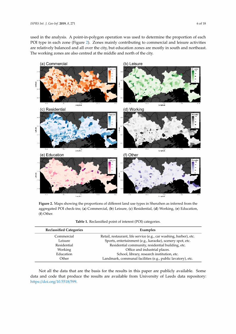
used in the analysis. A point-in-polygon operation was used to determine the proportion of eachPOI type in each zone (Figure 2). Zones mainly contributing to commercial and leisure activitiesare relatively balanced and all over the city, but education zones are mostly in south and northeast.The working zones are also centred at the middle and north of the city.
ISPRS Int. J. Geo-Inf. 2019, 8, x FOR PEER REVIEW 6 of 18
each zone (Figure 2). Zones mainly contributing to commercial and leisure activities are relatively balanced and all over the city, but education zones are mostly in south and northeast. The working zones are also centred at the middle and north of the city.
Not all the data that are the basis for the results in this paper are publicly available. Some data and code that produce the results are available from University of Leeds data repository: https://doi.org/10.5518/599.
Table 1. Reclassified point of interest (POI) categories.
Reclassified Categories Examples Commercial Retail, restaurant, life service (e.g., car washing, barber), etc.
Leisure Sports, entertainment (e.g., karaoke), scenery spot, etc. Residential Residential community, residential building, etc.
Working Office and industrial places. Education School, library, research institution, etc.
Other Landmark, communal facilities (e.g., public lavatory), etc.
Figure 2. Maps showing the proportions of different land use types in Shenzhen as inferred from the aggregated POI check-ins; (a) Commercial, (b) Leisure, (c) Residential, (d) Working, (e) Education, (f) Other.
4. Method
4.1. Temporal Trip Purpose Inference
Figure 2. Maps showing the proportions of different land use types in Shenzhen as inferred from theaggregated POI check-ins; (a) Commercial, (b) Leisure, (c) Residential, (d) Working, (e) Education,(f) Other.
Table 1. Reclassified point of interest (POI) categories.
Reclassified Categories Examples
Commercial Retail, restaurant, life service (e.g., car washing, barber), etc.Leisure Sports, entertainment (e.g., karaoke), scenery spot, etc.
Residential Residential community, residential building, etc.Working Office and industrial places.
Education School, library, research institution, etc.Other Landmark, communal facilities (e.g., public lavatory), etc.
Not all the data that are the basis for the results in this paper are publicly available. Somedata and code that produce the results are available from University of Leeds data repository:https://doi.org/10.5518/599.

ISPRS Int. J. Geo-Inf. 2019, 8, 271 7 of 18
4. Method
4.1. Temporal Trip Purpose Inference
The travel flows between metro stations from tap-ins and tap-outs provide limited informationabout how people interact with urban spaces—it is difficult to infer spatiotemporal patterns in trippurpose directly from travel records. This is an inherent shortcoming of anonymised SCD generatedfrom automated fare collection systems, which lack information about individual socioeconomicactivity that may be used to support inference about trip purpose. To overcome this, aggregated Weibocheck-in data were used to infer and weight potential land uses and activities in the areas aroundeach metro station. For each metro station, a service catchment area was defined by a 2500m buffer.This distance was used to represent a walking time of less than 30 minutes and a cycling time of around10 minutes. Please also note that the check-ins do not contain individual timestamp information—onlythe aggregated number is used.
For each catchment area, the number and type of different POI check-ins (residential, working,commercial, leisure, education) were determined. Figure 3a shows the proportion of different typeof check-ins using boxplot, and the correlations between different type of POI check-ins number andmetro trip amount are illustrated in Figure 3b. Overall, residential POIs contributed to most of thecheck-ins, followed by retail and working. Education has the lowest proportion on average (Figure 3a).All types of check-ins are found to have positive correlations with metro trip amount (Figure 3b),working presents the highest correlation, followed by commercial and residential.
ISPRS Int. J. Geo-Inf. 2019, 8, x FOR PEER REVIEW 7 of 18
The travel flows between metro stations from tap-ins and tap-outs provide limited information about how people interact with urban spaces—it is difficult to infer spatiotemporal patterns in trip purpose directly from travel records. This is an inherent shortcoming of anonymised SCD generated from automated fare collection systems, which lack information about individual socioeconomic activity that may be used to support inference about trip purpose. To overcome this, aggregated Weibo check-in data were used to infer and weight potential land uses and activities in the areas around each metro station. For each metro station, a service catchment area was defined by a 2500m buffer. This distance was used to represent a walking time of less than 30 minutes and a cycling time of around 10 minutes. Please also note that the check-ins do not contain individual timestamp information—only the aggregated number is used.
For each catchment area, the number and type of different POI check-ins (residential, working, commercial, leisure, education) were determined. Figure 3a shows the proportion of different type of check-ins using boxplot, and the correlations between different type of POI check-ins number and metro trip amount are illustrated in Figure 3b. Overall, residential POIs contributed to most of the check-ins, followed by retail and working. Education has the lowest proportion on average (Figure 3a). All types of check-ins are found to have positive correlations with metro trip amount (Figure 3b), working presents the highest correlation, followed by commercial and residential.
The trip purpose was then inferred by comparing the proportion of different kinds of POI check-in at traveller origin and destination catchment areas. For example, a trip from an area with predominantly residential POI check-ins to a one dominated by leisure POIs check-ins (e.g., an area with lots of check-ins at parks) is indicative of a passenger travelling from home to take part in leisure activities. Other trip purposes can be inferred from the change in POI check-in types between OD (Origin and Destination) metro station service catchments in a similar way.
Figure 3. (a) Distribution of the proportions of check-ins at different categories of POIs in metro service catchment; (b) correlation between POI check-ins and metro station trip amount.
People use the transit system to reach different places, for different purposes at different times of the day. In order to examine temporal variations in trip purpose, the operational metro service hours (6:00–23:00) were sliced into hourly intervals, and the aggregated total numbers of different categories of POI check-ins for each trip’s origin and destination metro station service catchment could be accumulated and compared.
To examine the differences between the land use groups further, a change rate was defined (Equation 1) to support a clear and deeper analysis of the temporal changes in trip origin and destination, R = 𝑂 𝐷max 𝑂 , 𝐷 100% (1)
where 𝑅 represents the change rate of land use category I, 𝑂 is the ratio of land use category i at the origin, and 𝐷 is the ratio of land use category i at the destination. The change rates provide an
Figure 3. (a) Distribution of the proportions of check-ins at different categories of POIs in metro servicecatchment; (b) correlation between POI check-ins and metro station trip amount.
The trip purpose was then inferred by comparing the proportion of different kinds of POI check-inat traveller origin and destination catchment areas. For example, a trip from an area with predominantlyresidential POI check-ins to a one dominated by leisure POIs check-ins (e.g., an area with lots ofcheck-ins at parks) is indicative of a passenger travelling from home to take part in leisure activities.Other trip purposes can be inferred from the change in POI check-in types between OD (Origin andDestination) metro station service catchments in a similar way.
People use the transit system to reach different places, for different purposes at different timesof the day. In order to examine temporal variations in trip purpose, the operational metro servicehours (6:00–23:00) were sliced into hourly intervals, and the aggregated total numbers of differentcategories of POI check-ins for each trip’s origin and destination metro station service catchment couldbe accumulated and compared.

ISPRS Int. J. Geo-Inf. 2019, 8, 271 8 of 18
To examine the differences between the land use groups further, a change rate was defined(Equation (1)) to support a clear and deeper analysis of the temporal changes in trip originand destination,
Ri =Oi −Di
max(Oi, Di)× 100% (1)
where Ri represents the change rate of land use category I, Oi is the ratio of land use category i atthe origin, and Di is the ratio of land use category i at the destination. The change rates provide anaggregate measure of how people travel from between land use areas in each time period. For example,if the rate for residential is positive, and the rate for working is negative, then this suggests thattravellers are leaving work and going home.
4.2. Traveler Division Based on Boarding Profile
Understanding the travel flows of different types (e.g., students, elderly) of travellers helpsuncover new insights into how individuals interact with and use urban space. However, sub-groupsof behaviours exist within the broad-scale groups that exhibit more nuanced spatio-temporalcharacteristics. The sub-groups are worthy of exploring because different travel behaviours areconsidered to be associated with travellers’ socioeconomic background [6] (e.g., income and educationlevel). Dividing transit users into detailed categories and understanding their travel patterns may helpto improve transport services. Rule-based approaches have been used within the literature [6,23,24] toextract certain travel behaviours (e.g., travel in early morning), but this relies heavily on formulatedand arbitrary rules. To overcome it, unsupervised learning can be applied to categorise travellersbased on their travel behaviour and help to uncover the sub-groups and their behaviour in transitsystems. To do this, boarding time profiles were created for each card holder, in which the hourly tripswere counted. For example, Figure 4 shows a hypothetical boarding time profile. This passenger madethree trips between 6:00–7:00 on Thursday with only two trips made in the other days. The profile is,in essence, a matrix of 5×24, with each number representing the count of tap-ins in 1-hour intervals.
ISPRS Int. J. Geo-Inf. 2019, 8, x FOR PEER REVIEW 8 of 18
aggregate measure of how people travel from between land use areas in each time period. For example, if the rate for residential is positive, and the rate for working is negative, then this suggests that travellers are leaving work and going home.
4.2. Traveler Division Based on Boarding Profile
Understanding the travel flows of different types (e.g., students, elderly) of travellers helps uncover new insights into how individuals interact with and use urban space. However, sub-groups of behaviours exist within the broad-scale groups that exhibit more nuanced spatio-temporal characteristics. The sub-groups are worthy of exploring because different travel behaviours are considered to be associated with travellers’ socioeconomic background [6] (e.g., income and education level). Dividing transit users into detailed categories and understanding their travel patterns may help to improve transport services. Rule-based approaches have been used within the literature [6,23,24] to extract certain travel behaviours (e.g., travel in early morning), but this relies heavily on formulated and arbitrary rules. To overcome it, unsupervised learning can be applied to categorise travellers based on their travel behaviour and help to uncover the sub-groups and their behaviour in transit systems. To do this, boarding time profiles were created for each card holder, in which the hourly trips were counted. For example, Figure 4 shows a hypothetical boarding time profile. This passenger made three trips between 6:00–7:00 on Thursday with only two trips made in the other days. The profile is, in essence, a matrix of 5×24, with each number representing the count of tap-ins in 1-hour intervals.
Figure 4. An example boarding time profile.
To evaluate the similarity between individual boarding time profiles, the average (mean) and variance value of boarding numbers for each time slot, were calculated for each user. This generates a total of 48 daily measures, which were used to characterise the temporal travel pattern of each individual i and to calculate a boarding time profile, 𝐶 , denoted as 𝐶 = [𝐴 , , 𝐴 , , ⋯ , 𝐴 , , 𝑉 , , 𝑉 , , ⋯ , 𝑉 , ] (2) where 𝐴 is the mean at the first-time slice and 𝑉 is the variance at the first-time slice. After extracting the 𝐶 , unsupervised learning (e.g., k-mean clustering) can be applied based the feature collection, thus dividing travellers into sub-groups.
5. Analysis and Results
The analysis sought to explore the temporality of trip patterns for different groups of users, comparing students against all travellers (Section 5.1), to infer trip purpose from the land uses associated with trip origins and destinations, comparing commuters, students and all travellers (Section 5.2) and to create profiles of the spatio-temporal behaviours of different sub-groups (Section 5.2.3).
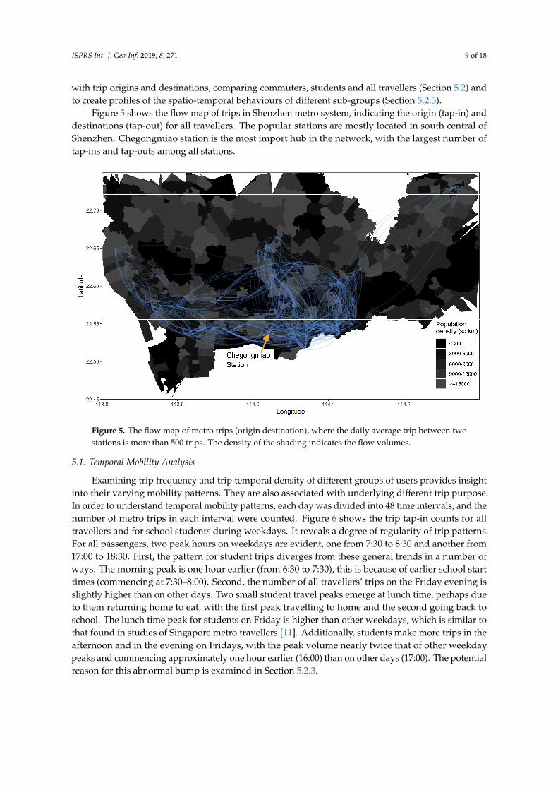
Figure 5 shows the flow map of trips in Shenzhen metro system, indicating the origin (tap-in) and destinations (tap-out) for all travellers. The popular stations are mostly located in south central of Shenzhen. Chegongmiao station is the most import hub in the network, with the largest number of tap-ins and tap-outs among all stations.
0
0
0
0
0
0
0
0
0
0
0
0
0
0
0
0
0
0
0
0
0
0
0
0
0
0
0
0
0
0
2
2
2
3
2
1
1
1
1
1
0
0
0
0
0
0
0
0
0
0
0
0
0
0
0
2
2
2
0
3
0
0
0
0
1
0
0
0
0
0
0
0
0
0
0
0
0
0
0
0
0
0
0
0
0
2
2
2
2
1
0
0
0
0
1
0
0
0
0
0
0
0
1
0
0
0
0
1
0
1
0
0
0
0
0
0
0
0
0
0
Monday
Tuesday
Wednesday
Thursday
Friday
0 5 10 15 20Hour
Day
0
1
2
3
TransactionAmount
Figure 4. An example boarding time profile.
To evaluate the similarity between individual boarding time profiles, the average (mean) andvariance value of boarding numbers for each time slot, were calculated for each user. This generatesa total of 48 daily measures, which were used to characterise the temporal travel pattern of eachindividual i and to calculate a boarding time profile, Ci, denoted as
Ci = [Ai,1, Ai,2, · · · , Ai,24, Vi,1, Vi,2, · · · , Vi,24] (2)
where Ai1 is the mean at the first-time slice and Vi1 is the variance at the first-time slice. After extractingthe Ci, unsupervised learning (e.g., k-mean clustering) can be applied based the feature collection, thusdividing travellers into sub-groups.
5. Analysis and Results
The analysis sought to explore the temporality of trip patterns for different groups of users,comparing students against all travellers (Section 5.1), to infer trip purpose from the land uses associated
ISPRS Int. J. Geo-Inf. 2019, 8, 271 9 of 18
with trip origins and destinations, comparing commuters, students and all travellers (Section 5.2) andto create profiles of the spatio-temporal behaviours of different sub-groups (Section 5.2.3).
Figure 5 shows the flow map of trips in Shenzhen metro system, indicating the origin (tap-in) anddestinations (tap-out) for all travellers. The popular stations are mostly located in south central ofShenzhen. Chegongmiao station is the most import hub in the network, with the largest number oftap-ins and tap-outs among all stations.ISPRS Int. J. Geo-Inf. 2019, 8, x FOR PEER REVIEW 9 of 18
Figure 5. The flow map of metro trips (origin destination), where the daily average trip between two stations is more than 500 trips. The density of the shading indicates the flow volumes.
5.1. Temporal Mobility Analysis
Examining trip frequency and trip temporal density of different groups of users provides insight into their varying mobility patterns. They are also associated with underlying different trip purpose. In order to understand temporal mobility patterns, each day was divided into 48 time intervals, and the number of metro trips in each interval were counted. Figure 6 shows the trip tap-in counts for all travellers and for school students during weekdays. It reveals a degree of regularity of trip patterns. For all passengers, two peak hours on weekdays are evident, one from 7:30 to 8:30 and another from 17:00 to 18:30. First, the pattern for student trips diverges from these general trends in a number of ways. The morning peak is one hour earlier (from 6:30 to 7:30), this is because of earlier school start times (commencing at 7:30–8:00). Second, the number of all travellers’ trips on the Friday evening is slightly higher than on other days. Two small student travel peaks emerge at lunch time, perhaps due to them returning home to eat, with the first peak travelling to home and the second going back to school. The lunch time peak for students on Friday is higher than other weekdays, which is similar to that found in studies of Singapore metro travellers [11]. Additionally, students make more trips in the afternoon and in the evening on Fridays, with the peak volume nearly twice that of other weekday peaks and commencing approximately one hour earlier (16:00) than on other days (17:00). The potential reason for this abnormal bump is examined in Section 5.2.3.
Figure 5. The flow map of metro trips (origin destination), where the daily average trip between twostations is more than 500 trips. The density of the shading indicates the flow volumes.
5.1. Temporal Mobility Analysis
Examining trip frequency and trip temporal density of different groups of users provides insightinto their varying mobility patterns. They are also associated with underlying different trip purpose.In order to understand temporal mobility patterns, each day was divided into 48 time intervals, and thenumber of metro trips in each interval were counted. Figure 6 shows the trip tap-in counts for alltravellers and for school students during weekdays. It reveals a degree of regularity of trip patterns.For all passengers, two peak hours on weekdays are evident, one from 7:30 to 8:30 and another from17:00 to 18:30. First, the pattern for student trips diverges from these general trends in a number ofways. The morning peak is one hour earlier (from 6:30 to 7:30), this is because of earlier school starttimes (commencing at 7:30–8:00). Second, the number of all travellers’ trips on the Friday evening isslightly higher than on other days. Two small student travel peaks emerge at lunch time, perhaps dueto them returning home to eat, with the first peak travelling to home and the second going back toschool. The lunch time peak for students on Friday is higher than other weekdays, which is similar tothat found in studies of Singapore metro travellers [11]. Additionally, students make more trips in theafternoon and in the evening on Fridays, with the peak volume nearly twice that of other weekdaypeaks and commencing approximately one hour earlier (16:00) than on other days (17:00). The potentialreason for this abnormal bump is examined in Section 5.2.3.

ISPRS Int. J. Geo-Inf. 2019, 8, 271 10 of 18ISPRS Int. J. Geo-Inf. 2019, 8, x FOR PEER REVIEW 10 of 18
Figure 6. The counts of trips for all travellers (a) and students (b) over five weekdays. The x-axis indicates half hour intervals, and the y-axis indicates the number of trips per 30 minutes.
5.2. Trip Purpose Pattern Analysis
5.2.1. Temporal Trip Purpose of Adult Travellers
Supplemental contextual information for travel flows can contribute to an understanding of trip purpose [8,32,33]. The analysis of temporal trip purpose utilised the methods described above. Recall that commuters were defined as those transport system users who travelled in the morning (6:00–11:00) for at least four out of the five weekdays. Their trips were compared with trips by all travellers, as shown in Figure 7. This indicates that the main changes in origin and destination proportions are driven by working and residential land uses during normal rush hour periods for both traveller groups, with similar relative increases in education, and that the volumes of trips from and to commercial land use remain constant through the day. However, it is difficult to infer important differences between these groups. To better interpret the temporal variation in travel purpose, the change rate R is calculated for the two broad-scale groups at each time interval.
Figure 7. The proportions of origin and destination associated with different land uses during weekdays for (a) all travellers and (b) commuters.
Figure 6. The counts of trips for all travellers (a) and students (b) over five weekdays. The x-axisindicates half hour intervals, and the y-axis indicates the number of trips per 30 minutes.
5.2. Trip Purpose Pattern Analysis
5.2.1. Temporal Trip Purpose of Adult Travellers
Supplemental contextual information for travel flows can contribute to an understanding oftrip purpose [8,32,33]. The analysis of temporal trip purpose utilised the methods described above.Recall that commuters were defined as those transport system users who travelled in the morning(6:00–11:00) for at least four out of the five weekdays. Their trips were compared with trips by alltravellers, as shown in Figure 7. This indicates that the main changes in origin and destinationproportions are driven by working and residential land uses during normal rush hour periods forboth traveller groups, with similar relative increases in education, and that the volumes of tripsfrom and to commercial land use remain constant through the day. However, it is difficult to inferimportant differences between these groups. To better interpret the temporal variation in travelpurpose, the change rate Ri is calculated for the two broad-scale groups at each time interval.
Figure 8 shows the change rate for different kinds of land use inferred from POI check-ins inorigins and destinations. Figure 8a allows the overall trip purposes for travellers to be inferred.People leave residential areas and to go to working and education areas in the morning rush hour,between 7:00–12:00, with the greatest value at 7:00. The trends decrease and converge at 11:00. Between12:00 and 14:00, the overall changes of trips between different land use areas are near to 0, withthe rate for working showing a small peak and the rate for residential a small trough, indicatingthat some travellers return home to eat and then go back for work. Then, from 14:00, the morningpattern is reversed, and the values for residential areas become positive while the values for workingand education areas change to negative as travellers begin to leave work and school to return home.There are some increases for commercial areas from 17:00 to 20:00. The change rate of leisure wasnegative (−12%) in the early morning, it increased and stayed steady around 0 at noon, and finallyreached around 10% after 17:00. Unlike the curve of commercial, change rate of leisure stayed around10% after 21:00, which implies that a certain number of metro travellers made their trip for leisureactivities at late night, while trips with commercial purpose are approaching zero (21:00), probably dueto the closing time of stores and malls (after 21:00).
For commuters (Figure 8b), the pattern is similar, but some subtle differences related to workingpatterns are observable. The flows from residential to working and to education are before 10:00.

ISPRS Int. J. Geo-Inf. 2019, 8, 271 11 of 18
They have a much sharper drop from their peaks to 0 before the midday. This indicates that the shiftsfrom residential to working are concentrated from 6:00 to 10:00 compared to similar changes for alltravellers (06:00–12:00). Travellers labelled as commuters are more likely to have a regular scheduledjob starting before 10:00.
ISPRS Int. J. Geo-Inf. 2019, 8, x FOR PEER REVIEW 10 of 18
Figure 6. The counts of trips for all travellers (a) and students (b) over five weekdays. The x-axis indicates half hour intervals, and the y-axis indicates the number of trips per 30 minutes.
5.2. Trip Purpose Pattern Analysis
5.2.1. Temporal Trip Purpose of Adult Travellers
Supplemental contextual information for travel flows can contribute to an understanding of trip purpose [8,32,33]. The analysis of temporal trip purpose utilised the methods described above. Recall that commuters were defined as those transport system users who travelled in the morning (6:00–11:00) for at least four out of the five weekdays. Their trips were compared with trips by all travellers, as shown in Figure 7. This indicates that the main changes in origin and destination proportions are driven by working and residential land uses during normal rush hour periods for both traveller groups, with similar relative increases in education, and that the volumes of trips from and to commercial land use remain constant through the day. However, it is difficult to infer important differences between these groups. To better interpret the temporal variation in travel purpose, the change rate R is calculated for the two broad-scale groups at each time interval.
Figure 7. The proportions of origin and destination associated with different land uses during weekdays for (a) all travellers and (b) commuters.
Figure 7. The proportions of origin and destination associated with different land uses during weekdaysfor (a) all travellers and (b) commuters.
ISPRS Int. J. Geo-Inf. 2019, 8, x FOR PEER REVIEW 11 of 18
Figure 8 shows the change rate for different kinds of land use inferred from POI check-ins in origins and destinations. Figure 8a allows the overall trip purposes for travellers to be inferred. People leave residential areas and to go to working and education areas in the morning rush hour, between 7:00–12:00, with the greatest value at 7:00. The trends decrease and converge at 11:00. Between 12:00 and 14:00, the overall changes of trips between different land use areas are near to 0, with the rate for working showing a small peak and the rate for residential a small trough, indicating that some travellers return home to eat and then go back for work. Then, from 14:00, the morning pattern is reversed, and the values for residential areas become positive while the values for working and education areas change to negative as travellers begin to leave work and school to return home. There are some increases for commercial areas from 17:00 to 20:00. The change rate of leisure was negative (−12%) in the early morning, it increased and stayed steady around 0 at noon, and finally reached around 10% after 17:00. Unlike the curve of commercial, change rate of leisure stayed around 10% after 21:00, which implies that a certain number of metro travellers made their trip for leisure activities at late night, while trips with commercial purpose are approaching zero (21:00), probably due to the closing time of stores and malls (after 21:00).
For commuters (Figure 8b), the pattern is similar, but some subtle differences related to working patterns are observable. The flows from residential to working and to education are before 10:00. They have a much sharper drop from their peaks to 0 before the midday. This indicates that the shifts from residential to working are concentrated from 6:00 to 10:00 compared to similar changes for all travellers (06:00–12:00). Travellers labelled as commuters are more likely to have a regular scheduled job starting before 10:00.
Different trip purpose can be interpreted from the temporal variation in change rates of different land use types. The most significant observations are working and residential. This is due to the higher degree of work-home spatial separation than other land use types in the city. Figure 2d also indicates that working-related POI check-ins are more spatially heterogenous and mainly clustered in several zones in the south.
Figure 8. Change rate for different categories of land use for (a) all travellers and (b) commuters.
5.2.2 Temporal Trip Purpose of Students
Figure 8. Change rate for different categories of land use for (a) all travellers and (b) commuters.
Different trip purpose can be interpreted from the temporal variation in change rates of differentland use types. The most significant observations are working and residential. This is due to the higherdegree of work-home spatial separation than other land use types in the city. Figure 2d also indicates

ISPRS Int. J. Geo-Inf. 2019, 8, 271 12 of 18
that working-related POI check-ins are more spatially heterogenous and mainly clustered in severalzones in the south.
5.2.2. Temporal Trip Purpose of Students
Trips undertaken by students were analysed to compare trips made on Monday to Thursdaywith those made on Fridays. Figure 6b highlights dramatic differences in afternoon trips on Fridays.The change rate (Equation (1)) was used to unpick variations in student trip purpose on Fridayafternoons and evenings. Because student trips are not related to work activities, work-related POIcheck-ins were excluded from the analysis. The results are shown in Figures 9 and 10. These indicatethat on Monday to Thursday, the change for residential dominates. Figures 9 and 10 indicate that themain trip purpose is returning home from school, but during Friday’s afternoon peak hour (from 16:00to 18:00) there is a dramatic decrease in the change rate for residential, which is negative around 16:00(Figure 10b). In contrast, change rate for commercial becomes the highest around 16:00. The switch ofposition of commercial and residential indicates that the main trip purpose for students during theFriday afternoon peak hour is “consuming in commercial areas” rather than returning home as onother weekdays. The rate for leisure also increases to positive from 16:00 to 18:00, suggesting that moretrips were made for the purposes of leisure activities compared to other weekdays.
ISPRS Int. J. Geo-Inf. 2019, 8, x FOR PEER REVIEW 12 of 18
Trips undertaken by students were analysed to compare trips made on Monday to Thursday with those made on Fridays. Figure 6b highlights dramatic differences in afternoon trips on Fridays. The change rate (Equation 1) was used to unpick variations in student trip purpose on Friday afternoons and evenings. Because student trips are not related to work activities, work-related POI check-ins were excluded from the analysis. The results are shown in Figures 9 and 10. These indicate that on Monday to Thursday, the change for residential dominates. Figures 9 and 10 indicate that the main trip purpose is returning home from school, but during Friday’s afternoon peak hour (from 16:00 to 18:00) there is a dramatic decrease in the change rate for residential, which is negative around 16:00 (Figure 10b). In contrast, change rate for commercial becomes the highest around 16:00. The switch of position of commercial and residential indicates that the main trip purpose for students during the Friday afternoon peak hour is “consuming in commercial areas” rather than returning home as on other weekdays. The rate for leisure also increases to positive from 16:00 to 18:00, suggesting that more trips were made for the purposes of leisure activities compared to other weekdays.
Figure 9. The proportions of origins and destinations associated with different land uses during weekdays for students on (a) Mondays to Thursdays, and (b) Fridays.
Figure 10. The change rates for different categories of land use for (a) Mondays to Thursdays, and (b) Fridays, for Student travellers.
5.2.3. Traveller Division and Detailed Temporal Trip Purpose
Figure 9. The proportions of origins and destinations associated with different land uses duringweekdays for students on (a) Mondays to Thursdays, and (b) Fridays.
ISPRS Int. J. Geo-Inf. 2019, 8, x FOR PEER REVIEW 12 of 18
Trips undertaken by students were analysed to compare trips made on Monday to Thursday with those made on Fridays. Figure 6b highlights dramatic differences in afternoon trips on Fridays. The change rate (Equation 1) was used to unpick variations in student trip purpose on Friday afternoons and evenings. Because student trips are not related to work activities, work-related POI check-ins were excluded from the analysis. The results are shown in Figures 9 and 10. These indicate that on Monday to Thursday, the change for residential dominates. Figures 9 and 10 indicate that the main trip purpose is returning home from school, but during Friday’s afternoon peak hour (from 16:00 to 18:00) there is a dramatic decrease in the change rate for residential, which is negative around 16:00 (Figure 10b). In contrast, change rate for commercial becomes the highest around 16:00. The switch of position of commercial and residential indicates that the main trip purpose for students during the Friday afternoon peak hour is “consuming in commercial areas” rather than returning home as on other weekdays. The rate for leisure also increases to positive from 16:00 to 18:00, suggesting that more trips were made for the purposes of leisure activities compared to other weekdays.
Figure 9. The proportions of origins and destinations associated with different land uses during weekdays for students on (a) Mondays to Thursdays, and (b) Fridays.
Figure 10. The change rates for different categories of land use for (a) Mondays to Thursdays, and (b) Fridays, for Student travellers.
5.2.3. Traveller Division and Detailed Temporal Trip Purpose
Figure 10. The change rates for different categories of land use for (a) Mondays to Thursdays, and (b)Fridays, for Student travellers.
ISPRS Int. J. Geo-Inf. 2019, 8, 271 13 of 18
5.2.3. Traveller Division and Detailed Temporal Trip Purpose
The final analysis sought to identify and compare behaviours sub-groups in terms of their patternsof travel using an example of student travellers. Student sub-groups (clusters) were identified fromsimilar temporal travel behaviour patterns.
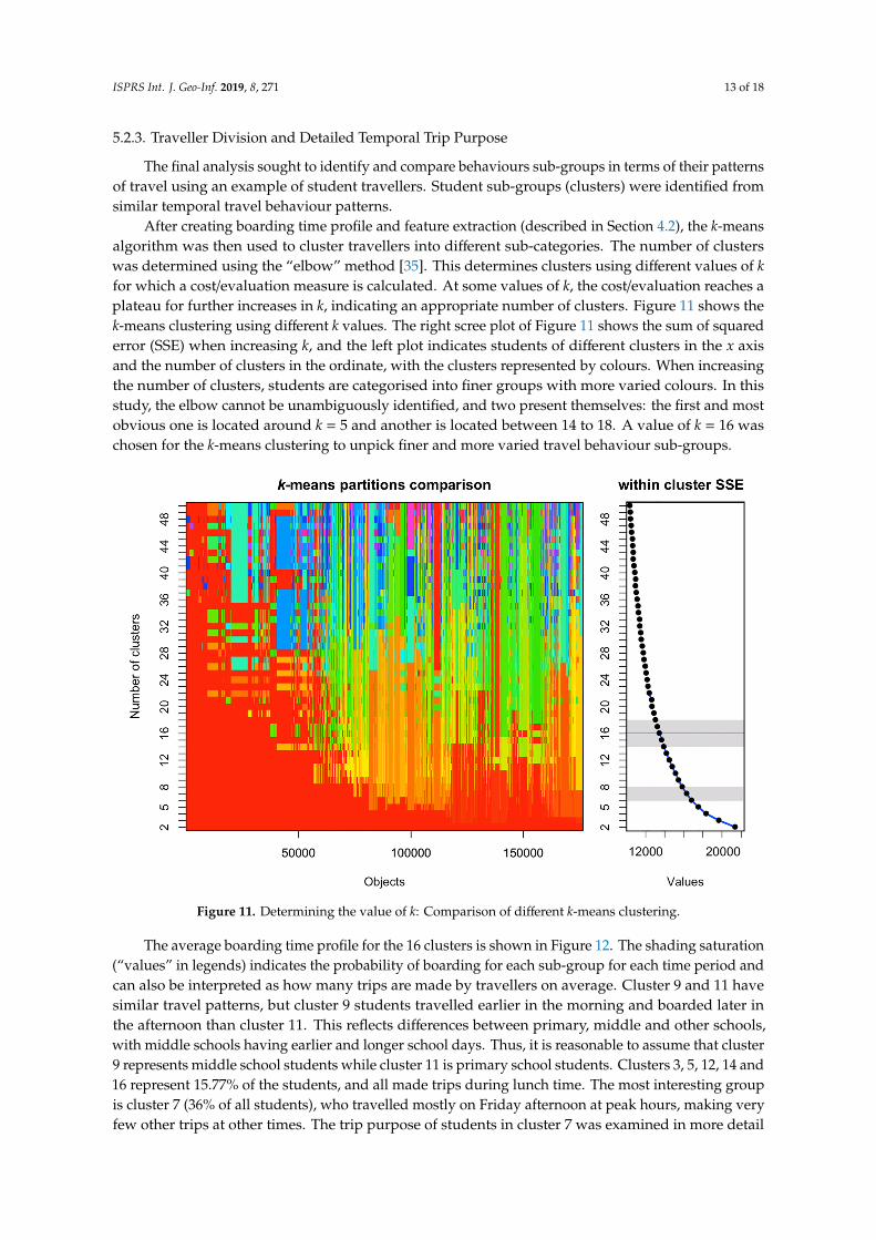
After creating boarding time profile and feature extraction (described in Section 4.2), the k-meansalgorithm was then used to cluster travellers into different sub-categories. The number of clusterswas determined using the “elbow” method [35]. This determines clusters using different values of kfor which a cost/evaluation measure is calculated. At some values of k, the cost/evaluation reaches aplateau for further increases in k, indicating an appropriate number of clusters. Figure 11 shows thek-means clustering using different k values. The right scree plot of Figure 11 shows the sum of squarederror (SSE) when increasing k, and the left plot indicates students of different clusters in the x axisand the number of clusters in the ordinate, with the clusters represented by colours. When increasingthe number of clusters, students are categorised into finer groups with more varied colours. In thisstudy, the elbow cannot be unambiguously identified, and two present themselves: the first and mostobvious one is located around k = 5 and another is located between 14 to 18. A value of k = 16 waschosen for the k-means clustering to unpick finer and more varied travel behaviour sub-groups.
ISPRS Int. J. Geo-Inf. 2019, 8, x FOR PEER REVIEW 13 of 18
The final analysis sought to identify and compare behaviours sub-groups in terms of their patterns of travel using an example of student travellers. Student sub-groups (clusters) were identified from similar temporal travel behaviour patterns.
After creating boarding time profile and feature extraction (described in Section 4.2), the k-means algorithm was then used to cluster travellers into different sub-categories. The number of clusters was determined using the “elbow” method [35]. This determines clusters using different values of k for which a cost/evaluation measure is calculated. At some values of k, the cost/evaluation reaches a plateau for further increases in k, indicating an appropriate number of clusters. Figure 11 shows the k-means clustering using different k values. The right scree plot of Figure 11 shows the sum of squared error (SSE) when increasing k, and the left plot indicates students of different clusters in the x axis and the number of clusters in the ordinate, with the clusters represented by colours. When increasing the number of clusters, students are categorised into finer groups with more varied colours. In this study, the elbow cannot be unambiguously identified, and two present themselves: the first and most obvious one is located around k = 5 and another is located between 14 to 18. A value of k = 16 was chosen for the k-means clustering to unpick finer and more varied travel behaviour sub-groups.
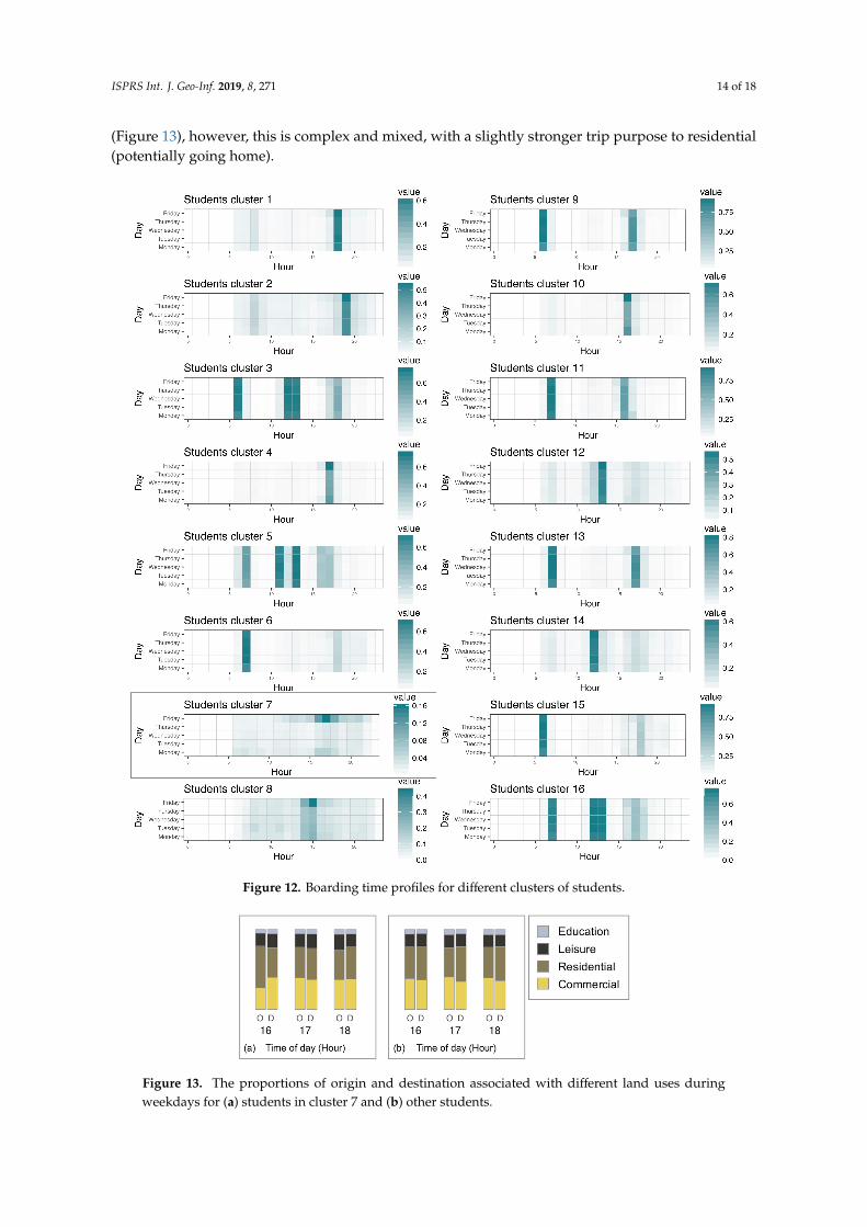
The average boarding time profile for the 16 clusters is shown in Figure 12. The shading saturation (“values” in legends) indicates the probability of boarding for each sub-group for each time period and can also be interpreted as how many trips are made by travellers on average. Cluster 9 and 11 have similar travel patterns, but cluster 9 students travelled earlier in the morning and boarded later in the afternoon than cluster 11. This reflects differences between primary, middle and other schools, with middle schools having earlier and longer school days. Thus, it is reasonable to assume that cluster 9 represents middle school students while cluster 11 is primary school students. Clusters 3, 5, 12, 14 and 16 represent 15.77% of the students, and all made trips during lunch time. The most interesting group is cluster 7 (36% of all students), who travelled mostly on Friday afternoon at peak hours, making very few other trips at other times. The trip purpose of students in cluster 7 was examined in more detail (Figure 13), however, this is complex and mixed, with a slightly stronger trip purpose to residential (potentially going home).
Figure 11. Determining the value of k: Comparison of different k-means clustering. Figure 11. Determining the value of k: Comparison of different k-means clustering.
The average boarding time profile for the 16 clusters is shown in Figure 12. The shading saturation(“values” in legends) indicates the probability of boarding for each sub-group for each time period andcan also be interpreted as how many trips are made by travellers on average. Cluster 9 and 11 havesimilar travel patterns, but cluster 9 students travelled earlier in the morning and boarded later inthe afternoon than cluster 11. This reflects differences between primary, middle and other schools,with middle schools having earlier and longer school days. Thus, it is reasonable to assume that cluster9 represents middle school students while cluster 11 is primary school students. Clusters 3, 5, 12, 14 and16 represent 15.77% of the students, and all made trips during lunch time. The most interesting groupis cluster 7 (36% of all students), who travelled mostly on Friday afternoon at peak hours, making veryfew other trips at other times. The trip purpose of students in cluster 7 was examined in more detail
ISPRS Int. J. Geo-Inf. 2019, 8, 271 14 of 18
(Figure 13), however, this is complex and mixed, with a slightly stronger trip purpose to residential(potentially going home).
ISPRS Int. J. Geo-Inf. 2019, 8, x FOR PEER REVIEW 14 of 18
The ratio associated with commercial for cluster 7 students rises significantly from 26.99% to 40.60% during 16:00–17:00 and is then steady during 17:00–19:00 compared to a drop from 40.75% to 35.21% during 17:00–18:00 and a drop throughout the whole period for other students (Figure 13b). In addition, the ratio associated with leisure for cluster 7 students increases during 16:00–18:00 then shows a decrease after 18:00 compared to a steady decrease for other students. The results indicate that many of those in cluster 7 take trips for commercial and leisure-related activities, which is different from other students who are mainly going to residential places.
Figure 12. Boarding time profiles for different clusters of students. Figure 12. Boarding time profiles for different clusters of students.ISPRS Int. J. Geo-Inf. 2019, 8, x FOR PEER REVIEW 15 of 18
Figure 13. The proportions of origin and destination associated with different land uses during weekdays for (a) students in cluster 7 and (b) other students.
6. Discussion
The results of this analysis infer travel behaviours for different groups of metro system users based on the temporal and spatial patterns of their trips, as recorded in smart card data (SCD) and linked to social media data. Land use at origin and destination locations were used to infer trip purpose, providing details and explanations of trips for different users at different times. The SCD allowed different groups of users to be identified based on their fare reductions (students), travel times (commuters) along with the land use derived from social media point of interest (POI) check-ins. These groups were further explored to identify different clusters of student travellers based on the temporal profile of their metro use.
This analysis of new sources of big data to examine travel behaviour addresses the obvious drawbacks and limitations of traditional travel survey data. The work generates similarity metrics for individual traveller profiles based on average trip times and their variance and is generalizable to other studies for user classification based on usage/interaction pattern. These may benefit from applying the per land use change rate approach and from transforming the travel data into “traveller profiles” to determine clusters of users. These could also be applied on repetitive timescales, for example. Moreover, this work used POI data to infer land use-related contextual information around metro stations. Potential land use activities were weighted by quantifying the number of POI check-ins at each POI to eliminate potential bias of treating all POIs equally. The proposed “change rate” measure is capable of supporting related visualisation analysis by providing clear trip purpose interpretation from flow-associated POIs.
Both the smart card data and social media check-in data may be subject to sampling bias, with the impacts of biases in the POI data potentially more serious. Here, only 70,000 POIs were used, a very limited proportion of the total number of POIs in Shenzhen, and their time stamps were between 2011 to 2014 and potentially subject to land use changes in that time. Therefore, a post-hoc validation exercise was undertaken to quantify the potential for bias in the Weibo check-in data. A sample of 1000 Weibo POIs were overlaid with reclassified Baidu map data. Here, the Baidu API was used to extract Baidu POI information in June 2018. The overall correspondence was 0.87, and the Type I errors rates for commercial, education, leisure, working and residential were 0.19, 0.14, 0.17, 0.04 and 0.17, respectively. These indicate the proportion of times a POI land use label used in this study was incorrect (false positives). These error rates suggest that the broad findings about trip destination and purpose are reliable but with varying degrees of uncertainty. The rapid development of Shenzhen may contribute to a high-speed change in urban land use of different areas, resulting in more uncertainty of using aggregated POI check-in data over long period. Ideally, using temporal matched contextual information can lead to a more accurate interpretation of local land use and trip purpose inference.
There are a number of limitations to this study and areas for further work. First, the analysis and identification of traveller segments, temporal variation in mobility patterns and trip purpose evaluated commuters and students against all travellers. These groups could be expanded, for example by examining the socioeconomic properties of the areas from which travellers originate (in the manner of geo-demographic classifications). This would support probabilistic inferences of more
Figure 13. The proportions of origin and destination associated with different land uses duringweekdays for (a) students in cluster 7 and (b) other students.

ISPRS Int. J. Geo-Inf. 2019, 8, 271 15 of 18
The ratio associated with commercial for cluster 7 students rises significantly from 26.99% to40.60% during 16:00–17:00 and is then steady during 17:00–19:00 compared to a drop from 40.75% to35.21% during 17:00–18:00 and a drop throughout the whole period for other students (Figure 13b).In addition, the ratio associated with leisure for cluster 7 students increases during 16:00–18:00 thenshows a decrease after 18:00 compared to a steady decrease for other students. The results indicate thatmany of those in cluster 7 take trips for commercial and leisure-related activities, which is differentfrom other students who are mainly going to residential places.
6. Discussion
The results of this analysis infer travel behaviours for different groups of metro system usersbased on the temporal and spatial patterns of their trips, as recorded in smart card data (SCD) andlinked to social media data. Land use at origin and destination locations were used to infer trippurpose, providing details and explanations of trips for different users at different times. The SCDallowed different groups of users to be identified based on their fare reductions (students), traveltimes (commuters) along with the land use derived from social media point of interest (POI) check-ins.These groups were further explored to identify different clusters of student travellers based on thetemporal profile of their metro use.
This analysis of new sources of big data to examine travel behaviour addresses the obviousdrawbacks and limitations of traditional travel survey data. The work generates similarity metrics forindividual traveller profiles based on average trip times and their variance and is generalizable to otherstudies for user classification based on usage/interaction pattern. These may benefit from applyingthe per land use change rate approach and from transforming the travel data into “traveller profiles”to determine clusters of users. These could also be applied on repetitive timescales, for example.Moreover, this work used POI data to infer land use-related contextual information around metrostations. Potential land use activities were weighted by quantifying the number of POI check-ins ateach POI to eliminate potential bias of treating all POIs equally. The proposed “change rate” measureis capable of supporting related visualisation analysis by providing clear trip purpose interpretationfrom flow-associated POIs.
Both the smart card data and social media check-in data may be subject to sampling bias, with theimpacts of biases in the POI data potentially more serious. Here, only 70,000 POIs were used, a verylimited proportion of the total number of POIs in Shenzhen, and their time stamps were between2011 to 2014 and potentially subject to land use changes in that time. Therefore, a post-hoc validationexercise was undertaken to quantify the potential for bias in the Weibo check-in data. A sample of1000 Weibo POIs were overlaid with reclassified Baidu map data. Here, the Baidu API was used toextract Baidu POI information in June 2018. The overall correspondence was 0.87, and the Type Ierrors rates for commercial, education, leisure, working and residential were 0.19, 0.14, 0.17, 0.04 and0.17, respectively. These indicate the proportion of times a POI land use label used in this study wasincorrect (false positives). These error rates suggest that the broad findings about trip destination andpurpose are reliable but with varying degrees of uncertainty. The rapid development of Shenzhen maycontribute to a high-speed change in urban land use of different areas, resulting in more uncertainty ofusing aggregated POI check-in data over long period. Ideally, using temporal matched contextualinformation can lead to a more accurate interpretation of local land use and trip purpose inference.
There are a number of limitations to this study and areas for further work. First, the analysis andidentification of traveller segments, temporal variation in mobility patterns and trip purpose evaluatedcommuters and students against all travellers. These groups could be expanded, for example byexamining the socioeconomic properties of the areas from which travellers originate (in the mannerof geo-demographic classifications). This would support probabilistic inferences of more nuancedand detailed trip purposes for a wider number of traveller groups and potentially would allowmore precise and explanatory analyses of travel behaviours, expanding the results presented here.Such analyses would also allow the potential biases in the representativeness of SCD to be quantified,

ISPRS Int. J. Geo-Inf. 2019, 8, 271 16 of 18
as travel smart cards may not be used equally by all social groups and offer a potential avenue tounderstand the sample biases associated with POI check-ins, which may over-represent particulartypes of activities, with, for example, people more likely to post micro-blogs while undertaking leisureactivities, compared to domestic ones. Second, land use is not static, rather multiple, alternate anddynamic land use attributes may be present [31] as the socioeconomic activities associated with anygiven location (origins and destinations in this study) may change over the course of a day. There isa need for studies of urban flows and dynamics to accommodate the dynamic nature of the conceptof land use, which may have specific functions at different times during the day. Here, the landuse from the POI data was inferred by the weighted aggregate check-ins to each POI in each zone.The timestamp of individual check-ins was not considered, which would allow the land use associatedwith each zone to be inferred dynamically. Such temporal refinements would extend and improveanalysis of trip purpose.
Smart card data in the metro system are only one kind of mobility big data that contain travelinformation of urban inhabitants. Other similar data include bike-sharing transactions and taxi triprecord. Smart card data of the bus and metro can generally capture flows and dynamics in mid- tolong-distance trips but may not be suitable for describing more localised travel and activities comparedto bike-sharing data. It should be noted that some other kinds of consumer data [36] can also be used toderive mobility-related information, some examples include cell phone tracking records, social mediadata (e.g., geo-tagged Twitter) and retail transaction records. The enumerated data all contain theirown set of shortcomings, for example, sampling bias, due to their varied attractiveness to differentkinds of urban inhabitants. Cell phone tracking records are considered to have high representativenessof users and may suffer least of all from the bias problem, but they have another shortcoming—thedata may fail to record every OD pair to represent travel flow because the location of the user is onlytracked when the phone is being used. These data can, to some extent, reveal urban dynamics andhow people interact and utilise urban space, but combining data from different sources may contributeto a more comprehensive picture of urban flows. Although varied in structure and spatiotemporalgranularity, such data and derived travel flows always benefit from external contextual information.Incorporating contextual data (e.g., land use) can lead to deeper understanding of the flows andactivities. The obtained insight on flows of individuals and groups of people at different time periodsalso reveals the complexity and diversity within city life.
7. Conclusions
New forms of smart card data present opportunities to generate new insights into the dynamics andpatterns of flows within cities. This study demonstrates how combining SCD with other context-richdata, such as social media data, are able to reveal the dynamics of mobility patterns associated withurban transit systems, and these vary amongst different social groups, supporting changes in urbanplanning. The study has demonstrated how linking such data can be analysed to infer: (a) Thebehaviours of different groups of travellers, (b) the socioeconomic activities that people undertakeand (c) how different groups (and sub-groups) identified in these ways are associated with differenttravel behaviours, trip purposes and socioeconomic activities. In so doing, this research addresses thedrawbacks and limitations associated with traditional travel survey data. It develops methods that aregeneralizable to other studies, supporting a more nuanced and detailed view of who, where, when andwhy people use city spaces. The approach uses social media POI data to semantically contextualiseinformation derived from the SCD to allow trip purpose to be inferred, to quantify spatiotemporalmobility patterns for different groups of travellers and to infer how their purposes of their journeyschange through the day. Future work will extend this research to explore the links between integratedtransportation trips, for example, via metro and bus, linked to use of new dockless bike schemes.Data from dockless bike sharing systems support spatiotemporal analyses of urban dynamics at a finergranularity than is possible through analysis of travel card or dock-based bike scheme. The increased

ISPRS Int. J. Geo-Inf. 2019, 8, 271 17 of 18
uptake of station-free travel data supports enhanced understandings of urban dynamics and travelpatterns over the “last mile” at much finer resolutions than has hitherto been possible.
Author Contributions: Conceptualization, Yuanxuan Yang and Alexis Comber; Methodology, Yuanxuan Yang,Andy Turner and Alexis Comber; Software, Yuanxuan Yang and Alexis Comber; Validation, Yuanxuan Yang andAlexis Comber; Formal Analysis, Yuanxuan Yang, Alison Heppenstall, Alexis Comber; Resources, YuanxuanYang; Writing-Original Draft Preparation, Yuanxuan Yang; Writing-Review & Editing, Alexis Comber, AlisonHeppenstall and Andy Turner; Visualization, Yuanxuan Yang; Supervision, Alexis Comber, Alison Heppenstalland Andy Turner.
Funding: This study is supported and funded by University of Leeds and Chinese Scholarship Council(201606420071), the Natural Environment Research Council (NE/S009124/1) and the Economic and Social ResearchCouncil Alan Turing research fellowship (ES/R007918/1).
Acknowledgments: The authors thank Transport Commission of Shenzhen Municipality, Future Transport Lab(Shenzhen) and Asia and Pacific Mathematical Contest in Modelling Committee for providing the smart carddataset and community boundary data. The authors thank the three reviewers whose comments and suggestionshelped improve and clarity this manuscript.
Conflicts of Interest: The authors declare no conflict of interest.
References
1. Batty, M. The New Science of Cities; MIT Press: Cambridge, UK, 2013.2. Pan, G.; Qi, G.; Wu, Z.; Zhang, D.; Li, S. Land-Use Classification Using Taxi GPS Traces. IEEE Trans. Intell.
Transp. Syst. 2013, 14, 113–123. [CrossRef]3. Collia, D.V.; Sharp, J.; Giesbrecht, L. The 2001 National Household Travel Survey: A look into the travel
patterns of older Americans. J. Saf. Res. 2003, 34, 461–470. [CrossRef]4. Brownstone, D.; Golob, T.F. The impact of residential density on vehicle usage and energy consumption.
J. Urban Econ. 2009, 65, 91–98. [CrossRef]5. Zhang, Z.; Mao, B.; Liu, M.; Chen, J.; Guo, J. Analysis of Travel Characteristics of Elders in Beijing. J. Transp.
Syst. Eng. Inf. Technol. 2007, 7, 11–20. [CrossRef]6. Long, Y.; Liu, X.; Zhou, J.; Chai, Y. Early birds, night owls, and tireless/recurring itinerants: An exploratory
analysis of extreme transit behaviors in Beijing, China. Habitat Int. 2016, 57, 223–232. [CrossRef]7. Pelletier, M.-P.; Trépanier, M.; Morency, C. Smart card data use in public transit: A literature review.
Transp. Res. Part C Emerg. Technol. 2011, 19, 557–568. [CrossRef]8. Liu, Y.; Liu, X.; Gao, S.; Gong, L.; Kang, C.; Zhi, Y.; Chi, G.; Shi, L. Social Sensing: A New Approach to
Understanding Our Socioeconomic Environments. Ann. Assoc. Am. Geogr. 2015, 105, 512–530. [CrossRef]9. Schmitt, G.; Klein, B.; König, R.; Schlaepfer, M.; Tunçer, B.; Buš, P. Big Data-Informed Urban Design, in Future
Cities Laboratory: Indicia 01; Cairns, S., Devisari, T., Eds.; Lars Müller Publishers: Zürich, Switzerland, 2017;pp. 103–113.
10. Bai, X.; Shi, P.; Liu, Y. Society: Realizing China’s urban dream. Nature 2014, 509, 158–160. [CrossRef][PubMed]
11. Zhong, C.; Manley, E.; Arisona, S.M.; Batty, M.; Schmitt, G. Measuring variability of mobility patterns frommultiday smart-card data. J. Comput. Sci. 2015, 9, 125–130. [CrossRef]
12. Ma, X.; Liu, C.; Wen, H.; Wang, Y.; Wu, Y.J. Understanding commuting patterns using transit smart card data.J. Transp. Geogr. 2017, 58, 135–145. [CrossRef]
13. Kim, J.; Corcoran, J.; Papamanolis, M. Route choice stickiness of public transport passengers: Measuringhabitual bus ridership behaviour using smart card data. Transp. Res. Part C Emerg. Technol. 2017, 83, 146–164.[CrossRef]
14. Zhou, J.; Sipe, N.; Ma, Z.; Mateo-Babiano, D.; Darchen, S. Monitoring transit-served areas with smartcarddata: A Brisbane case study. J. Transp. Geogr. 2017, 83, 1–11. [CrossRef]
15. Zhao, Z.; Koutsopoulos, H.N.; Zhao, J. Individual mobility prediction using transit smart card data.Transp. Res. Part C Emerg. Technol. 2018, 89, 19–34. [CrossRef]
16. Zhong, C.; Batty, M.; Manley, E.; Wang, J.; Wang, Z.; Chen, F.; Schmitt, G. Variability in Regularity: Mining TemporalMobility Patterns in London, Singapore and Beijing Using Smart-Card Data. PLoS ONE 2016, 11, e0149222. [CrossRef][PubMed]

ISPRS Int. J. Geo-Inf. 2019, 8, 271 18 of 18
17. Bagchi, M.; White, P.R. The potential of public transport smart card data. Transp. Policy 2005, 12, 464–474.[CrossRef]
18. Li, T.; Sun, D.; Jing, P.; Yang, K. Smart Card Data Mining of Public Transport Destination: A LiteratureReview. Information 2018, 9, 18–21. [CrossRef]
19. Huang, X.; Tan, J. Understanding spatio-temporal mobility patterns for seniors, child/student and adultusing smart card data. Int. Arch. Photogramm. Remote Sens. Spat. Inf. Sci. 2014, XL-1, 167–172.
20. Wang, M.; Zhou, J.; Long, Y.; Chen, F. Outside the ivory tower: Visualizing university students’ top transit-tripdestinations and popular corridors. Reg. Stud. Reg. Sci. 2016, 3, 202–206. [CrossRef]
21. Liu, Y.; Kang, C.; Gao, S.; Xiao, Y.; Tian, Y. Understanding intra-urban trip patterns from taxi trajectory data.J. Geogr. Syst. 2012, 14, 463–483. [CrossRef]
22. Wolf, J.; Guensler, R.; Bachman, W. Elimination of the Travel Diary: Experiment to Derive Trip Purpose fromGlobal Positioning System Travel Data. Transp. Res. Rec. J. Transp. Res. Board 2001, 1768, 125–134. [CrossRef]
23. Lee, S.G.; Hickman, M. Trip purpose inference using automated fare collection data. Public Transp. 2014, 6, 1–20.[CrossRef]
24. Devillaine, F.; Munizaga, M.; Trépanier, M. Detection of Activities of Public Transport Users by AnalyzingSmart Card Data. J. Transp. Res. Board 2012, 2276, 48–55. [CrossRef]
25. Medina, S.A.O. Inferring weekly primary activity patterns using public transport smart card data and ahousehold travel survey. Travel Behav. Soc. 2018, 12, 93–101. [CrossRef]
26. Liu, L.; Hou, A.; Biderman, A.; Ratti, C.; Chen, J. Understanding individual and collective mobility patternsfrom smart card records: A case study in Shenzhen. In Proceedings of the 12th International IEEE Conferenceon Intelligent Transportation Systems (ITSC), St. Louis, MO, USA, 4–7 October 2009; pp. 1–6.
27. Yue, M.; Kang, C.; Andris, C.; Qin, K.; Liu, Y.; Meng, Q. Understanding the interplay between bus, metro,and cab ridership dynamics in Shenzhen, China. Trans. GIS 2018, 22, 855–871. [CrossRef]
28. Chen, C.; Gong, H.; Lawson, C.; Bialostozky, E. Evaluating the feasibility of a passive travel survey collectionin a complex urban environment: Lessons learned from the New York City case study. Transp. Res. Part APolicy Pract. 2010, 44, 830–840. [CrossRef]
29. Chung, E.-H.; Shalaby, A. A trip reconstruction tool for GPS-based personal travel surveys. Transp. Plan.Technol. 2005, 28, 381–401. [CrossRef]
30. Bohte, W.; Maat, K. Deriving and validating trip purposes and travel modes for multi-day GPS-based travelsurveys: A large-scale application in the Netherlands. Transp. Res. Part C Emerg. Technol. 2009, 17, 285–297.[CrossRef]
31. Fisher, P.; Comber, A.J.; Wadsworth, R.A.R. Land use and land cover: Contradiction or complement.In Re-Presenting GIS; Fisher, P., Unwin, D., Eds.; Wiley: Chichester, UK, 2005; pp. 85–98.
32. Rashidi, T.H.; Abbasi, A.; Maghrebi, M.; Hasan, S.; Waller, T.S. Exploring the capacity of social media data formodelling travel behaviour: Opportunities and challenges. Transp. Res. Part C Emerg. Technol. 2017, 75, 197–211.[CrossRef]
33. Liu, Y.; Wang, F.; Xiao, Y.; Gao, S. Urban land uses and traffic ‘source-sink areas’: Evidence from GPS-enabledtaxi data in Shanghai. Landsc. Urban Plan. 2012, 106, 73–87. [CrossRef]
34. Zhao, J.; Qu, Q.; Zhang, F.; Xu, C.; Liu, S. Spatio-Temporal Analysis of Passenger Travel Patterns in MassiveSmart Card Data. IEEE Trans. Intell. Transp. Syst. 2017, 18, 3135–3146. [CrossRef]
35. Tibshirani, R.; Walther, G.; Hastie, T. Estimating the number of clusters in a data set via the gap statistic. J. R.Stat. Soc. B 2001, 63, 411–423. [CrossRef]
36. Birkin, M. Spatial data analytics of mobility with consumer data. J. Transp. Geogr. 2019, 76, 245–253.[CrossRef]
© 2019 by the authors. Licensee MDPI, Basel, Switzerland. This article is an open accessarticle distributed under the terms and conditions of the Creative Commons Attribution(CC BY) license (http://creativecommons.org/licenses/by/4.0/).