welcome to the united states: self-selection of … · welcome to the united states: self-selection...

Welcome to the United States: Self-selection of Puerto Rican Migrants

Kathryn Haiying Li

Dr. Seth Sanders, Faculty Advisor

Dr. Marjorie McElroy, Honors Workshop Professor

Honors Thesis submitted in partial fulfillment of the requirements for Graduation with Distinction in Economics in Trinity College of Duke University.

Duke University

Durham, North Carolina 2011

2

Acknowledgement

I am grateful to Dr. Marjorie McElroy and Dr. Seth Sanders for their continuous guidance and

support throughout the year. I would also like to thank Bicheng Yang and Songman Kang for

their help with Stata; my classmates Becky Agostino, Steven Seidel, and Josh Silverman in the

Honors Workshop; and my friends Linda Li, Robert Won, and Yiwen Zhu for their invaluable

peer reviews.

3

Abstract

I analyze the characteristics of Puerto Rican migrants and non-migrants to make two

contributions to existing literature: (1) The empirical analysis demonstrates that contrary to

previous studies done on only working men, the 1990 data inclusive of women and non-working

individuals actually support a positive self-selection in which highly skilled Puerto Ricans

migrate to the U.S. The 2000 results, however, do provide strong support for negative self-

selection in which the less skilled migrate. (2) The predicted, counterfactual wages for migrant

and non-migrant counterparts reveal that wage differentials are not the only consideration in their

decision to migrate.

JEL classification: J10, J11

Keywords: Self-selection, Roy Model, Migrant, Puerto Rico

4

Table of Contents

Page

Sections

I. Introduction 5

II. Literature Review 6

III. Roy Model and Self-selection Theory 7

IV. Decennial Census Data 10

V. Empirical Methodology 11

VI. Results and Discussion 22

VII. Conclusion 32

Appendices

A. Figure 33

B. Additional Stata Output Tables 34

Bibliography 39

5

I. Introduction

The United States constitutes the single largest recipient of immigrants,1with a total of

approximately 35 million immigrants residing in the U.S. in 2000 (Francis, 2007). Consequently,

the demographic composition of the U.S. is projected to become increasingly diverse, in which

population growth will be driven predominantly by the growth of the Hispanic population.2

To gain a better understanding of the impending demographic shift, it is particularly

interesting to analyze the attributes of Puerto Rican migrants because their skill structures are

well documented. Furthermore, the fact that Puerto Ricans hold U.S. citizenship makes them one

of the most mobile migrant populations with a high percentage of returnees. The size and

composition of migration inflow and outflow can be attributed to social and economic disparities

between the U.S. and Puerto Rico (referred to as PR from hereon after) (Ramos, 1992).

It is instructive to analyze the characteristics of both Puerto Rican migrants and non-

migrants to determine self-selection. In essence, positive self-selection occurs when highly

skilled workers from the sending country migrate to the receiving country and negative self-

selection occurs when low skilled workers migrate.

In this paper, I examine the self-selection of Puerto Rican migrants and predict potential

wages for their migrant or non-migrant counterparts had their decisions been reversed.3It

1 Back in 1940, one million legal immigrants entered the U.S. every ten years; by 2002, the same number of immigrants was being admitted every year (Borjas, 2008). 2 See Figure 8 in Appendix A on page 33 for the Hispanic population growth in the U.S. from 1994 to 2008. The National Center for Health Statistics reported that while the fertility rate of non-Hispanic white women has fallen to 1.847, that of Hispanic women has remained at 2.824 (Preston & Hartnett, 2008). If the current trend of fertility and migration continues, the Hispanic-origin population would contribute to approximately 45% of the population growth from 2010 to 2030 and 60% from 2030 to 2050; by 2050, the proportional shares of the population is projected to shift to less than 50.1% non-Hispanic White, 24.4% of Hispanic origin, 14.6% Black, 8% Asian and Pacific Islander, and 5% all other races (Projected Population of the United States, by Race and Hispanic Origin: 2000 to 2050, 2004). 3 Wages are predicted for stayers had they returned to PR, for returnees had they stayed in the U.S., for recent migrant had they remained in PR, and for non-migrants had they migrated.

6

proceeds as follows: Section II provides an overview of current literature on Puerto Rican

migration; Section III explains the Roy model and self-selection theory which are fundamental to

the theoretical framework; Section IV delineates the decennial census data used for analysis;

Section V presents the empirical methodology using data drawn from the 1990 and 2000 U.S.

and PR Censuses, and provides an overview of Heckman’s Two-stage Estimation Method;

Section VI discusses the empirical findings, in which 1990 data corroborate with positive self-

selection while 2000 data support negative self-selection; finally, Section VII concludes with the

implications of the results.

II. Literature Review

George Borjas (1987), a leading economist and professor at Harvard Kennedy School,

predicted positive self-selection for migrants from relatively rich and developed countries and

negative self-selection for those from relatively poor and less developed countries. Borjas and

Bratsberg (1996) used administrative data from the Immigration and Naturalization Service (INS)

and the 1980 U.S. Census to motivate the self-selection theory. The conclusions derived from the

INS may have been incomprehensive because INS includes statistics on only permanent

residents, excluding data on migrants who entered via student visa, business visa, or visitor visa.

Borjas (2007) provided substantiation for negative self-selection of Puerto Rican migrants

by demonstrating that the least educated were motivated to migrate to the U.S. because they

could earn higher wages in the U.S. than in PR. However, the empirical analysis was restricted to

only men who reported wages, which did not account for sample selection bias.

Fernando A. Ramos (1992) used data from the 1980 U.S. and PR Censuses to present

results reflecting Borjas’s conclusions, reinforcing the view that Puerto Ricans were negatively

7

self-selected. Ramos concluded that Puerto Rican migrants were less educated than non-migrants

and that returnees were more educated than those who stayed in the U.S. He found that average

returnees earned 13.3% less than non-migrants and that average recent migrants earned 18% less

than older migrants. His findings further supported the migration pattern proposed by Borjas,

that returnees intensified the negative self-selection characterized by recent migrants.

Nevertheless, Ramos also restricted empirical analysis to only male workers aged 20-64. Once

again, such analysis did not account for sample selection bias that arises from leaving out women

and non-working individuals.

At present, the existing literature on Puerto Rican migration is incomprehensive. It

primarily covers migration prior to 1990 and includes empirical analysis done on employed men.

This paper not only provides an extension of past studies by looking at 1990 and 2000 Heckit

regression results for all working and non-working individuals but also predicts counterfactual

wages for their migrant or non-migrant counterparts.

III. Roy Model and Self-selection Theory

The theory regarding the skills of migrants assumes that individuals who find it

worthwhile to migrate are not randomly selected. Rather, the decision to migrate depends on the

income distribution in both the sending and receiving countries. The relationship of the two

motivates individuals with particular demographic and socioeconomic characteristics to leave

their home.

The empirical analysis of self-selection theory for migrants is motivated by Borjas’s

modification of the Roy model. The Roy model of self-selection is a framework for analyzing

comparative advantage and was originally used to examine the occupational choice between

8

hunter and fisherman. Borjas first adapted the two-sector Roy model into the self-selection

theory of migration to the U.S. He proposed that individuals compare expected wages in the U.S.

with their wages at home. Having made such appraisals, individuals who anticipate higher

earnings in the U.S. than at home choose to migrate. The theoretical implications indicate that

self-selection depends on the relative income inequality4of the sending and receiving countries,

or in this situation, the sending territory PR and receiving mainland, the U.S.

Recall that self-selection is traditionally categorized into either positive or negative self-

selection in which positive self-selection occurs when highly skilled workers migrate and

negative self-selection occurs when low skilled workers migrate. In both cases, variance of

wages in the sending and receiving countries plays a critical role in determining the type of self-

selection. To analyze the role of variance, assume that the probability density functions of

ln(wage) for both sending and receiving countries are symmetric with the same means.

Also assume that there exists a positive correlation between skill and wage in both

countries. For ease of argument, assume that a worker in top decile of the skill distribution would

be in the top decile of the ln(wage) distribution. Likewise, assume that a worker in the bottom

decile of the skill distrubition would be in the bottom decile of the ln(wage) distribution. In

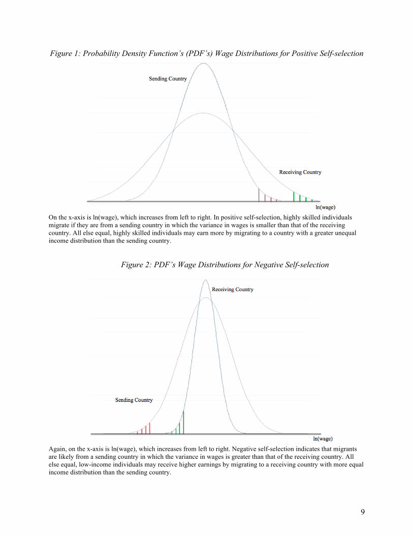
Figures 1 and 2, the shaded segments cut off an area of 0.10 (10%). The role of variance can be

seen as follows:

4 Income inequality is generally measured by the Gini coefficient, which is named after the Italian economist Corrado Gini. The Gini coefficient is derived from a statistical formula and describes the income inequality of a country, where 0 indicates absolute equality (everyone in the country has equal income) and 1 represents absolute inequality (one person has all the income in the country). For more information, visit http://web.worldbank.org/WBSITE/EXTERNAL/TOPICS/EXTPOVERTY/EXTPA/0,,contentMDK:20238991~menuPK:492138~pagePK:148956~piPK:216618~theSitePK:430367,00.html

9

Figure 1: Probability Density Function’s (PDF’s) Wage Distributions for Positive Self-selection

On the x-axis is ln(wage), which increases from left to right. In positive self-selection, highly skilled individuals migrate if they are from a sending country in which the variance in wages is smaller than that of the receiving country. All else equal, highly skilled individuals may earn more by migrating to a country with a greater unequal income distribution than the sending country.

Figure 2: PDF’s Wage Distributions for Negative Self-selection

Again, on the x-axis is ln(wage), which increases from left to right. Negative self-selection indicates that migrants are likely from a sending country in which the variance in wages is greater than that of the receiving country. All else equal, low-income individuals may receive higher earnings by migrating to a receiving country with more equal income distribution than the sending country.

10

Given the flexibility of the decision for migrants to return to their home countries after a

temporary stay in the U.S., an interesting pattern of self-selection may arise. The pattern predicts

that the return migration process intensifies the self-selection that characterizes the migrants in

the U.S. Returnees are classified as marginal migrants such that those who remain in the U.S. are

“the best of the best” if positively selected or “the worst of the worst” if negatively selected

(Borjas and Bratsberg, 1996).

IV. Decennial Census Data

Data used in this paper come from the Integrated Public Use Micro-data Series (IPUMS),

which collects and distributes U.S. Census data from 1850 to 2009 and PR Census data from

1910 to 2009.

The main advantage of using decennial censuses is the ease of selecting mutually

exclusive and exhaustive population groups from nationally representative samples. Because the

censuses ask individuals to list their place of residence five years ago, the destination country

and previous place of residence are known. Thus individuals can be categorized as stayers, recent

migrants, returnees, and non-migrants. Furthermore, the U.S. and PR Censuses are especially

useful for comparison given that the majority of the questions asked are identical.

The primary disadvantage from using census data is the limited choice of variables; that

certain questions are omitted limits variable selection for more comprehensive regressions. For

instance, experience is a variable left out of census data, so education is used instead as a proxy

to measure skill.

11

V. Empirical Methodology

In order to compare the population samples from censuses, I include both working and

non-working men and women. Moreover, I restrict the age group to 21-55 based on the range of

prime working age: individuals under 21 may still be in school while those over 55 are

approaching retirement and thus, less likely to work because of other age-related circumstances

than younger individuals.

Unlike previous studies, this paper stratifies the migrant and non-migrant groups into four

mutually exclusive and exhaustive groups. Figures 3, 4, and 5 on the following pages illustrate

the case for the 2000 Puerto Rican migrant and non-migrant population samples. Figure 3 shows

the year of migration and Figure 4 depicts the place of residence for the respective migrant and

non-migrant groups in the ten-year span, 1990-2000. Because the U.S. and PR Censuses do not

track the number of entries for individuals who migrate back and forth between the U.S. and PR,

the last year of entry is taken as the year of migration. Furthermore, the place of residence is

known only five years prior to the census year, which restricts the scope of this study to that

point in time for reference.

Using data extracted from the 2000 U.S. Census and the corresponding 2000 PR Census, I

have partitioned Puerto Ricans into migrants and non-migrants. Migrants in turn, are partitioned

into stayers, returnees, and recent migrants. I compare two groups of Puerto Ricans who were

either in the U.S. or PR in 1995. For example, Figure 6 on page 14 shows that recent migrants

from the U.S. Census are compared to non-migrants from the PR Census, stayers from the U.S.

Census are compared to returnees from the PR Census, and finally, stayers are compared to

recent migrants (both are from the U.S. Census).

12

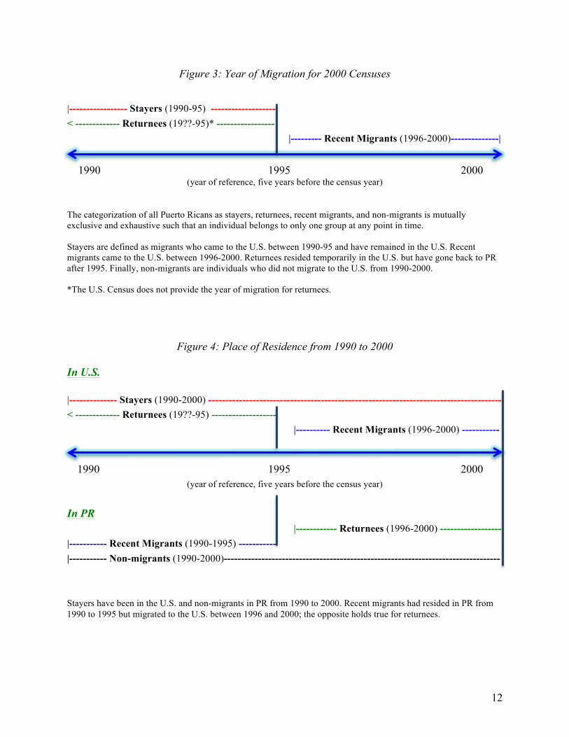
Figure 3: Year of Migration for 2000 Censuses

|----------------- Stayers (1990-95) ------------------- < ------------- Returnees (19??-95)* ----------------- |--------- Recent Migrants (1996-2000)--------------|

1990 1995 2000 (year of reference, five years before the census year)

The categorization of all Puerto Ricans as stayers, returnees, recent migrants, and non-migrants is mutually exclusive and exhaustive such that an individual belongs to only one group at any point in time. Stayers are defined as migrants who came to the U.S. between 1990-95 and have remained in the U.S. Recent migrants came to the U.S. between 1996-2000. Returnees resided temporarily in the U.S. but have gone back to PR after 1995. Finally, non-migrants are individuals who did not migrate to the U.S. from 1990-2000. *The U.S. Census does not provide the year of migration for returnees.

Figure 4: Place of Residence from 1990 to 2000

In U.S. |-------------- Stayers (1990-2000) -------------------------------------------------------------------------------------- < ------------- Returnees (19??-95) ------------------- |---------- Recent Migrants (1996-2000) ----------- 1990 1995 2000

(year of reference, five years before the census year) In PR |------------ Returnees (1996-2000) ------------------ |----------- Recent Migrants (1990-1995) ----------- |----------- Non-migrants (1990-2000)---------------------------------------------------------------------------------

Stayers have been in the U.S. and non-migrants in PR from 1990 to 2000. Recent migrants had resided in PR from 1990 to 1995 but migrated to the U.S. between 1996 and 2000; the opposite holds true for returnees.

13

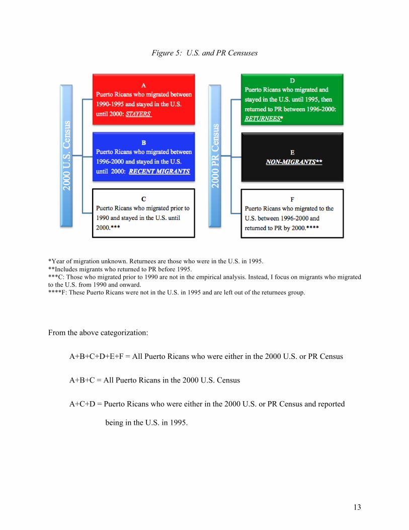
Figure 5: U.S. and PR Censuses

*Year of migration unknown. Returnees are those who were in the U.S. in 1995. **Includes migrants who returned to PR before 1995. ***C: Those who migrated prior to 1990 are not in the empirical analysis. Instead, I focus on migrants who migrated to the U.S. from 1990 and onward. ****F: These Puerto Ricans were not in the U.S. in 1995 and are left out of the returnees group.

From the above categorization:

A+B+C+D+E+F = All Puerto Ricans who were either in the 2000 U.S. or PR Census

A+B+C = All Puerto Ricans in the 2000 U.S. Census

A+C+D = Puerto Ricans who were either in the 2000 U.S. or PR Census and reported

being in the U.S. in 1995.

14

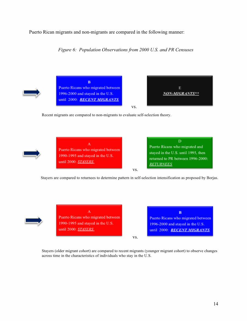
Puerto Rican migrants and non-migrants are compared in the following manner:

Figure 6: Population Observations from 2000 U.S. and PR Censuses

vs.

Recent migrants are compared to non-migrants to evaluate self-selection theory.

vs.

Stayers are compared to returnees to determine pattern in self-selection intensification as proposed by Borjas.

vs.

Stayers (older migrant cohort) are compared to recent migrants (younger migrant cohort) to observe changes across time in the characteristics of individuals who stay in the U.S.

15

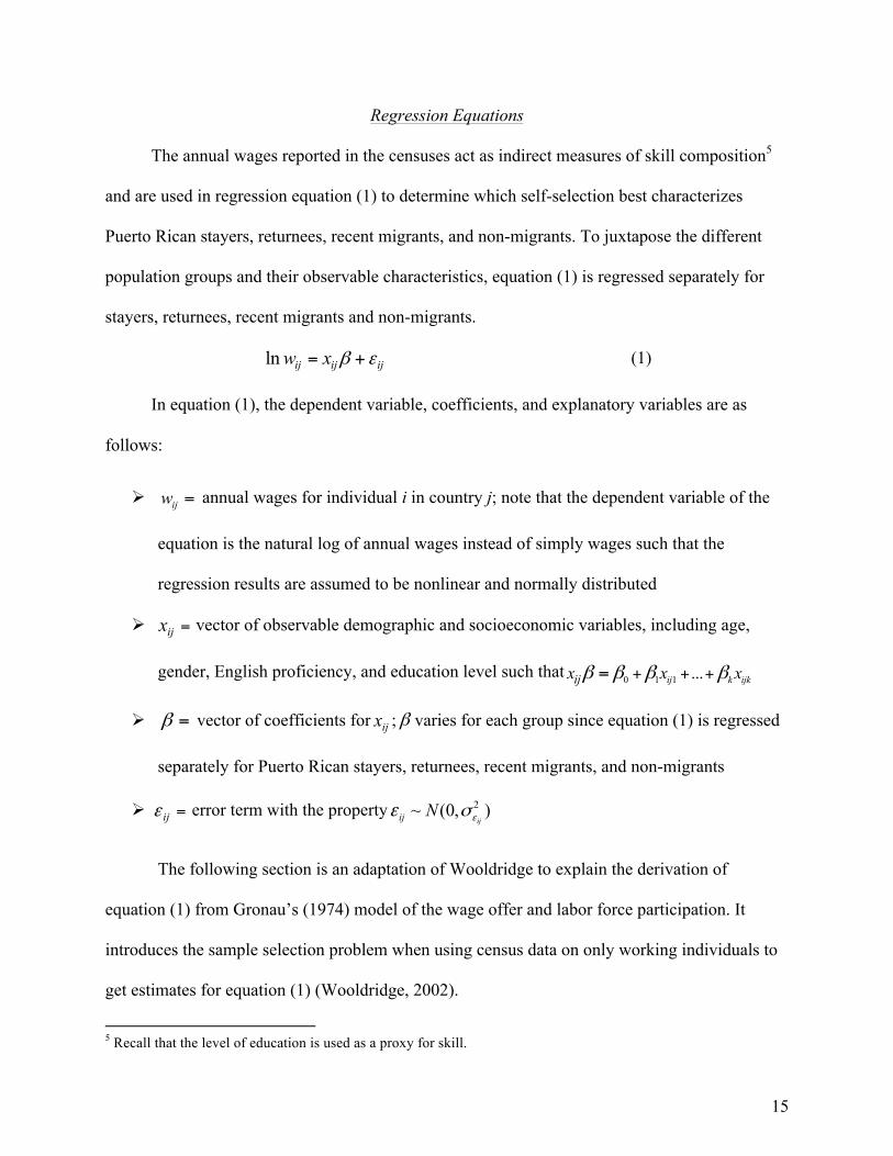
Regression Equations

The annual wages reported in the censuses act as indirect measures of skill composition5

and are used in regression equation (1) to determine which self-selection best characterizes

Puerto Rican stayers, returnees, recent migrants, and non-migrants. To juxtapose the different

population groups and their observable characteristics, equation (1) is regressed separately for

stayers, returnees, recent migrants and non-migrants.

(1)

In equation (1), the dependent variable, coefficients, and explanatory variables are as

follows:

Ø ijw = annual wages for individual i in country j; note that the dependent variable of the

equation is the natural log of annual wages instead of simply wages such that the

regression results are assumed to be nonlinear and normally distributed

Ø ijx = vector of observable demographic and socioeconomic variables, including age,

gender, English proficiency, and education level such that 0 1 1 ...ij k ijkijx x xβ β β β+ + +=

Ø vector of coefficients for ; varies for each group since equation (1) is regressed

separately for Puerto Rican stayers, returnees, recent migrants, and non-migrants

Ø ijε = error term with the property 2~ (0, )ijij N εσε

The following section is an adaptation of Wooldridge to explain the derivation of

equation (1) from Gronau’s (1974) model of the wage offer and labor force participation. It

introduces the sample selection problem when using census data on only working individuals to

get estimates for equation (1) (Wooldridge, 2002).

5 Recall that the level of education is used as a proxy for skill.

ln ij ij ijw x β ε= +

β = ijx β

16

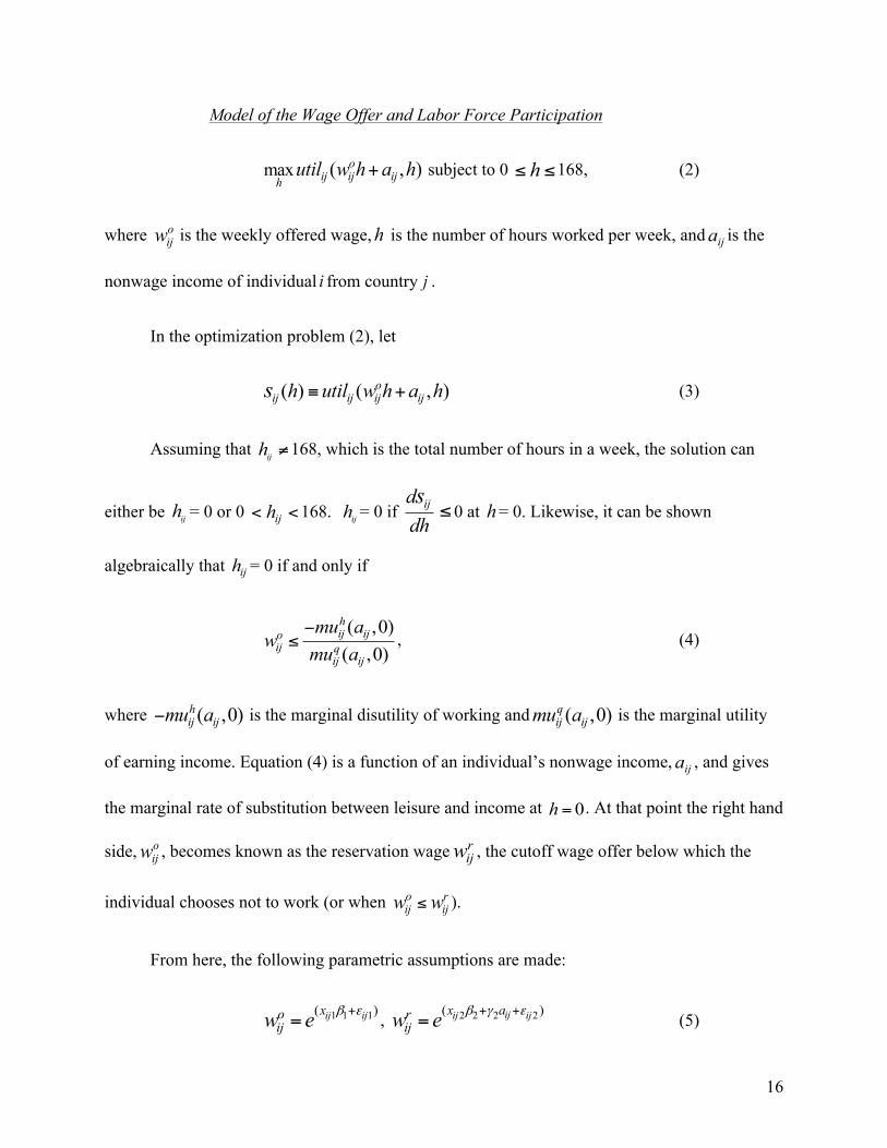
Model of the Wage Offer and Labor Force Participation

max ( , )oij ij ijh

util w h a h+ subject to 0 h≤ ≤168, (2)

where oijw is the weekly offered wage,h is the number of hours worked per week, and ija is the

nonwage income of individual i from country j .

In the optimization problem (2), let

( ) ( , )oij ij ij ijh util w h a hs ≡ + (3)

Assuming that ijh ≠168, which is the total number of hours in a week, the solution can

either be = 0 or 0 ijh< <168. ijh = 0 if ijddhs≤0 at h= 0. Likewise, it can be shown

algebraically that ijh = 0 if and only if

( ,0)( ,0)

hij ijo

ij qij ij

mu aw

mu a−

≤ , (4)

where ( ,0)hij ijmu a− is the marginal disutility of working and ( ,0)q

ij ijmu a is the marginal utility

of earning income. Equation (4) is a function of an individual’s nonwage income, ija , and gives

the marginal rate of substitution between leisure and income at 0h = . At that point the right hand

side, oijw , becomes known as the reservation wage r

ijw , the cutoff wage offer below which the

individual chooses not to work (or when o rij ijw w≤ ).

From here, the following parametric assumptions are made:

1 1 1( )ij ijxoijw e β ε+= , 2 2 2 2( )ijij ijx ar

ijw e β γ ε+ += (5)

ijh

17

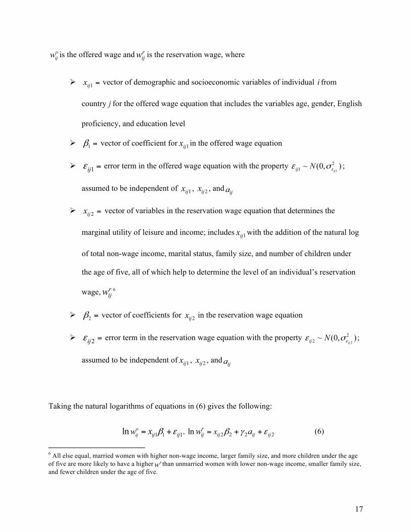
is the offered wage and is the reservation wage, where

Ø 1ijx = vector of demographic and socioeconomic variables of individual i from

country j for the offered wage equation that includes the variables age, gender, English

proficiency, and education level

Ø 1β = vector of coefficient for 1ijx in the offered wage equation

Ø 1ijε = error term in the offered wage equation with the property 1

21 ~ (0, )

ijij N εσε ;

assumed to be independent of , , and

Ø 2ijx = vector of variables in the reservation wage equation that determines the

marginal utility of leisure and income; includes 1ijx with the addition of the natural log

of total non-wage income, marital status, family size, and number of children under

the age of five, all of which help to determine the level of an individual’s reservation

wage, rijw 6

Ø 2β = vector of coefficients for 2ijx in the reservation wage equation

Ø 2ijε = error term in the reservation wage equation with the property 2

22 ~ (0, )

ijij N εσε ;

assumed to be independent of , , and

Taking the natural logarithms of equations in (6) gives the following:

11 1ln oij ij ijw x β ε= + , ln r

ijw = 2 2 2 2ijij ijx aβ γ ε+ + (6)

6 All else equal, married women with higher non-wage income, larger family size, and more children under the age of five are more likely to have a higher rw than unmarried women with lower non-wage income, smaller family size, and fewer children under the age of five.

oijw r

ijw

1ijx 2ijx ija

1ijx 2ijx ija

18

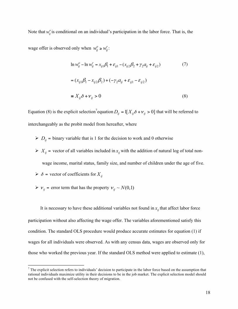
Note that oijw is conditional on an individual’s participation in the labor force. That is, the

wage offer is observed only when o rij ijw w≥ :

1 1 1 2 2 2 2ln ln ( )o rij ij ijij ij ij ijx xw w aβ ε β γ ε− = −+ + + (7)

21 1 2 2 1 2( ) ( )ijij ij ij ijx x aγβ β ε ε= − + − + −

0ij ijX δ ν≡ + > (8)

Equation (8) is the explicit selection7equation 1[ 0]ij ij ijD X δ ν= + > that will be referred to

interchangeably as the probit model from hereafter, where

Ø ijD = binary variable that is 1 for the decision to work and 0 otherwise

Ø ijX = vector of all variables included in ijx with the addition of natural log of total non-

wage income, marital status, family size, and number of children under the age of five.

Ø δ = vector of coefficients for

Ø ijν = error term that has the property ~ (0,1)ij Nν

It is necessary to have these additional variables not found in that affect labor force

participation without also affecting the wage offer. The variables aforementioned satisfy this

condition. The standard OLS procedure would produce accurate estimates for equation (1) if

wages for all individuals were observed. As with any census data, wages are observed only for

those who worked the previous year. If the standard OLS method were applied to estimate (1),

7 The explicit selection refers to individuals’ decision to participate in the labor force based on the assumption that rational individuals maximize utility in their decisions to be in the job market. The explicit selection model should not be confused with the self-selection theory of migration.

ijX

ijx

19

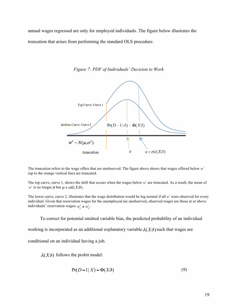
annual wages regressed are only for employed individuals. The figure below illustrates the

truncation that arises from performing the standard OLS procedure.

Figure 7: PDF of Individuals’ Decision to Work

The truncation refers to the wage offers that are unobserved. The figure above shows that wages offered below rw(up to the orange vertical line) are truncated. The top curve, curve 1, shows the shift that occurs when the wages below rw are truncated. As a result, the mean of

rw is no longer µ but ( )Xµ σλ δ+ . The lower curve, curve 2, illustrates that the wage distribution would be log normal if all rw were observed for every individual. Given that reservation wages for the unemployed are unobserved, observed wages are those at or above individuals’ reservation wages: o r

ij ijw w≥ .

To correct for potential omitted variable bias, the predicted probability of an individual

working is incorporated as an additional explanatory variable ( )Xδλ such that wages are

conditional on an individual having a job.

( )Xδλ follows the probit model:

Pr( 1| ) ( )D X Xδ= =Φ (9)

20

Equation (8), 1[ 0]ij ij ijD X δ ν= + > , in conjunction with equation (1), ln ij ij ijw x β ε= + ,

constitute Heckman’s Two-stage Estimation Method. Whether or not the earnings are observed

depends on the binary variable, namely labor force participation ijD where ijD = 1 if the

individual decides to work and ijD = 0 otherwise.

Heckman’s Two-stage Estimation Method

Heckman’s Two-stage Estimation Method, also known as Heckit (the combination of

Heckman and “it” from the probit procedure) corrects the sample selection bias.

First, using the entire population, estimates of δ are obtained through the probit model.

Second, the estimated inverse Mills ratio ( )Xλ λ δ∧ ∧≡ 8is calculated to regress lnw on X and λ

∧

to get consistent and approximately normally distributedβ∧

.

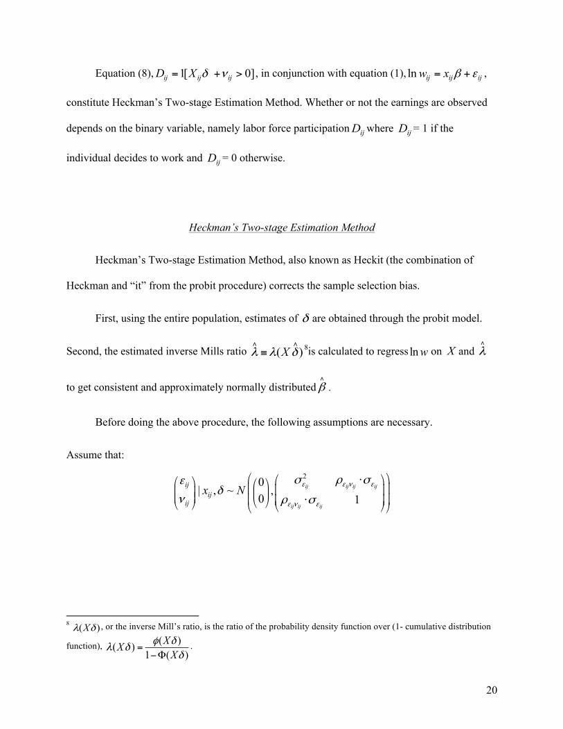
Before doing the above procedure, the following assumptions are necessary.

Assume that:

2

,0

| , ~0 1

ij ij ij ij

ij ij ij

ijij

ijx N ε ε ν ε

ε ν ε

σ ρ σεδ

ν ρ σ

⎛ ⎞⎛ ⎞⎛ ⎞ ⎛ ⎞⎜ ⎟⎜ ⎟⎜ ⎟ ⎜ ⎟⎜ ⎟ ⎜ ⎟⎜ ⎟⎝ ⎠⎝ ⎠ ⎝ ⎠⎝ ⎠

⋅

⋅

8 ( )Xλ δ , or the inverse Mill’s ratio, is the ratio of the probability density function over (1- cumulative distribution

function), ( )( )1 ( )

XXX

φ δλ δδ

=−Φ

.

21

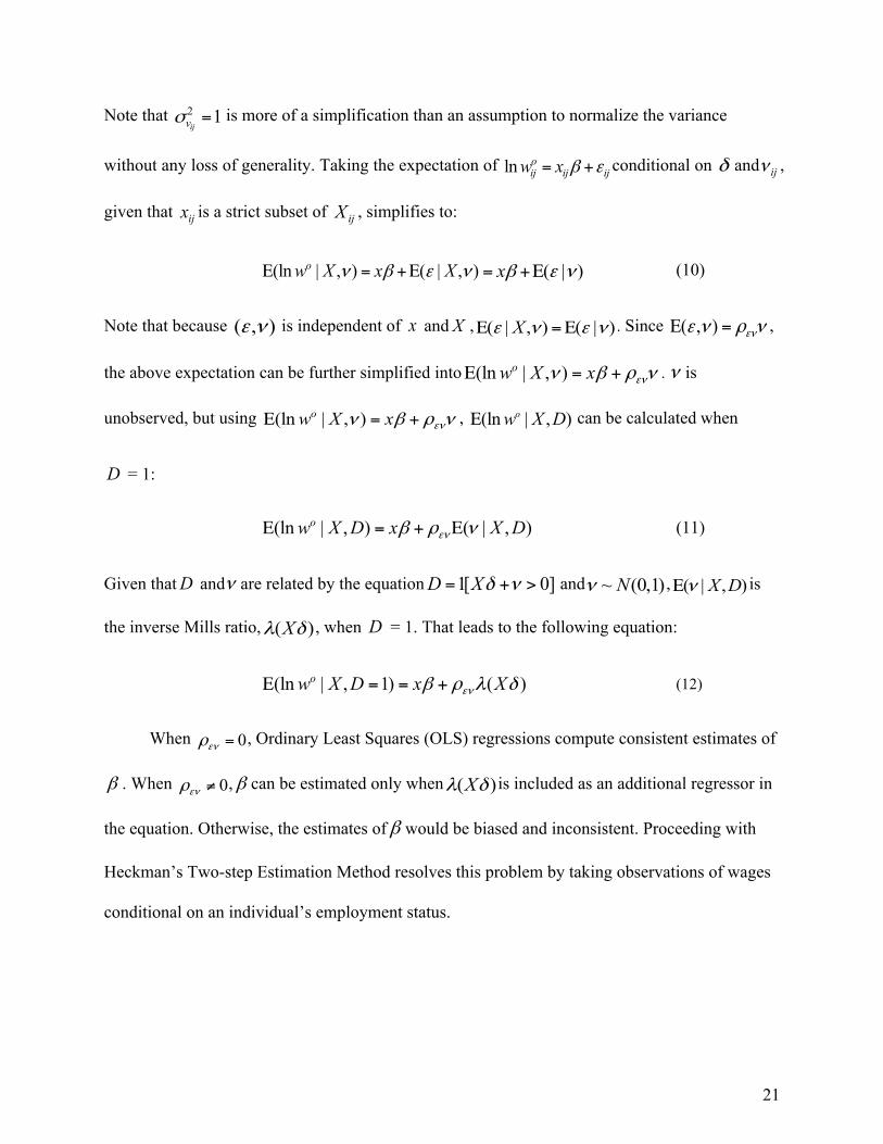
Note that 2 1ijvσ =

is more of a simplification than an assumption to normalize the variance

without any loss of generality. Taking the expectation of ln oij ij ijw x β ε= + conditional on δ and ijν ,

given that ijx is a strict subset of ijX , simplifies to:

(ln | , ) ( | , )ow X x Xν β ε νΕ = +Ε ( | )xβ ε ν= +Ε (10)

Note that because ( , )ε ν is independent of x and X , ( | , ) ( | )Xε ν ε νΕ =Ε . Since ( , ) ενε ν ρ νΕ = ,

the above expectation can be further simplified into (ln | , )ow X x ενν β ρ νΕ = + . ν is

unobserved, but using (ln | , )ow X x ενν β ρ νΕ = + , (ln | , )ow X DΕ can be calculated when

D = 1:

(ln | , ) ( | , )ow X D x X Dενβ ρ νΕ = + Ε (11)

Given thatD and are related by the equation 1[ 0]D Xδ ν= + > and ~ (0,1)Nν , ( | , )X DνΕ is

the inverse Mills ratio, ( )Xλ δ , when = 1. That leads to the following equation:

(ln | , 1) ( )ow X D x Xενβ ρ λ δΕ = = + (12)

When 0ενρ = , Ordinary Least Squares (OLS) regressions compute consistent estimates of

β . When 0ενρ ≠ ,β can be estimated only when ( )Xλ δ is included as an additional regressor in

the equation. Otherwise, the estimates of would be biased and inconsistent. Proceeding with

Heckman’s Two-step Estimation Method resolves this problem by taking observations of wages

conditional on an individual’s employment status.

ν

D

β

22

VI. Results and Discussion

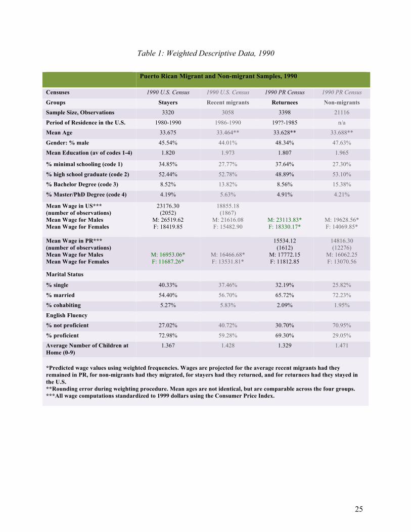
Table 1 on the page 25 summarizes the weighted descriptive data9in which the individual

frequency weights of the recent migrants, returnees, and non-migrants have been standardized to

match the age distribution of the Puerto Rican stayers in the U.S. in 1990. Such weighting

eliminates potential aging effects10by equating the age distributions across the four groups.

Moreover, it allows for the analysis of individuals of the same mean age, which is accurate up to

two significant figures.

The first row reports the census. Second row indicates the population group. Third row

gives the number of observations for stayers, recent immigrants, returnees, and non-migrants.

The next row depicts the period of residence in the U.S. for each group. Note that mean

education is calculated as an average of codes 1 through 4, where 1 represents minimal schooling,

2 for high school graduates (including those with some college education but no Bachelor

Degree), 3 for those with Bachelor Degrees, and 4 for those with Master or PhD Degrees.

All annual wages have been deflated to 1999 dollars. They are calculated as an average

for the overall working population, and then separately for men and women because of the

substantial wage differential between them. The wages with an asterisk are the predicted

earnings for the corresponding groups: for stayers had they returned, for returnees had they

stayed in the U.S., for recent migrants had they remained in PR, and for non-migrants had they

9 Table 6 in Appendix B on page 35 is the 1990 non-weighted descriptive data. 10 Aging effects describes the phenomenon in which older generations are likely to be less educated than the younger generations because educational opportunities have become increasingly accessible over the years.

23

migrated. Wages are first regressed on the weighted11reference group and then predicted for the

corresponding group by incorporating the characteristics of that group.12

The marital status of individuals are divided into three categories: those who are single or

living alone, those married, and those unmarried but cohabiting with a partner. The next rows

indicate the level of English fluency and are categorized as either proficient or not proficient.

The last row indicates the average number of children at home.

Overall, the 1990 Censuses data indicate that the stayers have the highest average earnings

followed by recent migrants, such that migrants in the U.S. generally earn more than those in PR.

Due in part to assimilation and selection effects, stayers have the highest percentage of proficient

English speakers while non-migrants have the lowest. In addition, stayers have the highest

percentage of single households while recent migrants have the most cohabitating households.

Non-migrants have the most married households with a corresponding highest average number

of children.

Stayers exhibit the second lowest average level of education. Their wages, however, are

highest among the four groups: the average 33-year-old male stayers earn $26,519.62 per year

while the average 33-year-old female stayers earn $18,419.85 per year. Counterfactual, predicted

wages indicate that the average 33-year-old female stayer would have earned around

$11,687.2613had she returned to PR. Thus, the comparison of the actual wages with predicted

11 See Table 5 in Appendix B on page 34 for the weighting method. Note that the census is already weighted. Because it is only a 5% sample of the entire population, all individuals in the census are weighted according to their probability of being selected such that the data can be representative of the population as a whole. 12 For instance, the predicted wages for the recent migrants are their potential earnings had they not migrated. They are projected in the following manner: (1) non-migrants are weighted according to the age distribution of the stayers; (2) wages are then regressed on non-migrants; (3) finally, the predict command in Stata projects wages for recent migrants by incorporating their demographic and socioeconomic characteristics into the wage estimation. 13 The predicted wage for the average 33-year-old Puerto Rican is of course, unobservable in reality due to the impossibility of having individuals reside in two countries at the same time- but it can be calculated using the aforementioned predicted wage procedure on top of this page.

24

income for stayers and recent migrants reveals that their decisions to reside in the U.S. are

economically rational. The same comparisons done with the actual and predicted wages for

returnees and non-migrants indicate otherwise. Consequently, wage differentials are not the only

consideration in individuals’ decisions to migrate. While many other factors go into determining

individuals’ wage and decision to migrate, the predicted wages are nonetheless informative for

preliminary comparison purposes.

In terms of education level, average 33-year-old recent migrants have the highest among

the four groups with 52.78% high school graduates, 13.82% college graduates, and 5.63% with

Master or PhD Degrees. On the contrary, average returnees have the lowest mean education.

This finding contradicts both negative self-selection and self-selection intensification theory as

proposed by Borjas. Instead of having low skilled individuals migrate and the highly skilled

returning, the results indicate that the least-educated return to PR. In comparing recent migrants

with non-migrants, the results support positive self-selection, which is inconsistent with Borjas’s

and Ramos’s findings.

25

Table 1: Weighted Descriptive Data, 1990

Puerto Rican Migrant and Non-migrant Samples, 1990

Censuses 1990 U.S. Census 1990 U.S. Census 1990 PR Census 1990 PR Census

Groups Stayers Recent migrants Returnees Non-migrants

Sample Size, Observations 3320 3058 3398 21116

Period of Residence in the U.S. 1980-1990 1986-1990 19??-1985 n/a

Mean Age 33.675 33.464** 33.628** 33.688**

Gender: % male 45.54% 44.01% 48.34% 47.63%

Mean Education (av of codes 1-4) 1.820 1.973 1.807 1.965

% minimal schooling (code 1) 34.85% 27.77% 37.64% 27.30%

% high school graduate (code 2) 52.44% 52.78% 48.89% 53.10%

% Bachelor Degree (code 3) 8.52% 13.82% 8.56% 15.38%

% Master/PhD Degree (code 4) 4.19% 5.63% 4.91% 4.21%

Mean Wage in US*** (number of observations) Mean Wage for Males Mean Wage for Females

23176.30 (2052)

M: 26519.62 F: 18419.85

18855.18 (1867)

M: 21616.08 F: 15482.90

M: 23113.83* F: 18330.17*

M: 19628.56* F: 14069.85*

Mean Wage in PR*** (number of observations) Mean Wage for Males Mean Wage for Females

M: 16953.06* F: 11687.26*

M: 16466.68* F: 13531.81*

15534.12 (1612)

M: 17772.15 F: 11812.85

14816.30 (12276)

M: 16062.25 F: 13070.56

Marital Status

% single 40.33% 37.46% 32.19% 25.82%

% married 54.40% 56.70% 65.72% 72.23%

% cohabiting 5.27% 5.83% 2.09% 1.95%

English Fluency

% not proficient 27.02% 40.72% 30.70% 70.95%

% proficient 72.98% 59.28% 69.30% 29.05%

Average Number of Children at Home (0-9)

1.367 1.428 1.329 1.471

*Predicted wage values using weighted frequencies. Wages are projected for the average recent migrants had they remained in PR, for non-migrants had they migrated, for stayers had they returned, and for returnees had they stayed in the U.S. **Rounding error during weighting procedure. Mean ages are not identical, but are comparable across the four groups. ***All wage computations standardized to 1999 dollars using the Consumer Price Index.

26

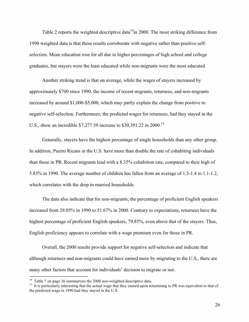
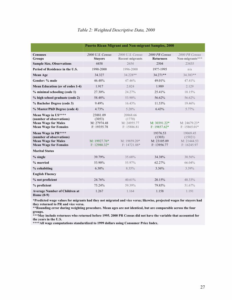
Table 2 reports the weighted descriptive data14in 2000. The most striking difference from

1990 weighted data is that these results corroborate with negative rather than positive self-

selection. Mean education rose for all due to higher percentages of high school and college

graduates, but stayers were the least educated while non-migrants were the most educated.

Another striking trend is that on average, while the wages of stayers increased by

approximately $700 since 1990, the income of recent migrants, returnees, and non-migrants

increased by around $1,000-$5,000, which may partly explain the change from positive to

negative self-selection. Furthermore, the predicted wages for returnees, had they stayed in the

U.S., show an incredible $7,277.39 increase to $30,391.22 in 2000.15

Generally, stayers have the highest percentage of single households than any other group.

In addition, Puerto Ricans in the U.S. have more than double the rate of cohabiting individuals

than those in PR. Recent migrants lead with a 8.35% cohabition rate, compared to their high of

5.83% in 1990. The average number of children has fallen from an average of 1.3-1.4 to 1.1-1.2,

which correlates with the drop in married households.

The data also indicate that for non-migrants, the percentage of proficient English speakers

increased from 29.05% in 1990 to 51.67% in 2000. Contrary to expectations, returnees have the

highest percentage of proficient English speakers, 79.85%, even above that of the stayers. Thus,

English proficiency appears to correlate with a wage premium even for those in PR.

Overall, the 2000 results provide support for negative self-selection and indicate that

although returnees and non-migrants could have earned more by migrating to the U.S., there are

many other factors that account for individuals’ decision to migrate or not. 14 Table 7 on page 36 summarizes the 2000 non-weighted descriptive data. 15 It is particularly interesting that the actual wage that they earned upon returnining to PR was equivalent to that of the predicted wage in 1990 had they stayed in the U.S.

27

Table 2: Weighted Descriptive Data, 2000

Puerto Rican Migrant and Non-migrant Samples, 2000

Censuses 2000 U.S. Census 2000 U.S. Census 2000 PR Census 2000 PR Census Groups Stayers Recent migrants Returnees Non-migrants*** Sample Size, Observations 4458 2654 2504 23435


Mean Age 34.327 34.228** 34.271** 34.383**

Gender: % male 46.48% 47.46% 49.01% 47.41%






Mean Wage in US**** (number of observations) Mean Wage for Males Mean Wage for Females

23881.09 (3053)

M: 27974.48 F: 19355.78

20868.66 (1770)

M: 24955.77 F: 15886.81

M: 30391.22* F: 19857.62*

M: 24679.23*

F: 15865.01*

Mean Wage in PR**** (number of observations) Mean Wage for Males Mean Wage for Females

M: 19927.76* F: 12980.32*

M: 19859.20* F: 14721.88*

19376.53 (1303)

M: 23105.09 F: 13956.77

19069.45 (15021)

M: 21444.53 F: 16245.97

Marital Status

% single 39.79% 35.68% 34.38% 30.56%

% married 53.90% 55.97% 62.27% 66.04%

% cohabiting 6.30% 8.35% 3.36% 3.39%

English Fluency

% not proficient 24.76% 40.61% 20.15% 48.33%

% proficient 75.24% 59.39% 79.85% 51.67%


1.267 1.164 1.158 1.191

*Predicted wage values for migrants had they not migrated and vice versa; likewise, projected wages for stayers had they returned to PR and vice versa. **Rounding error during weighting procedure. Mean ages are not identical, but are comparable across the four groups. ***May include returnees who returned before 1995. 2000 PR Census did not have the variable that accounted for the years in the U.S. ****All wage computations standardized to 1999 dollars using Consumer Price Index.

28

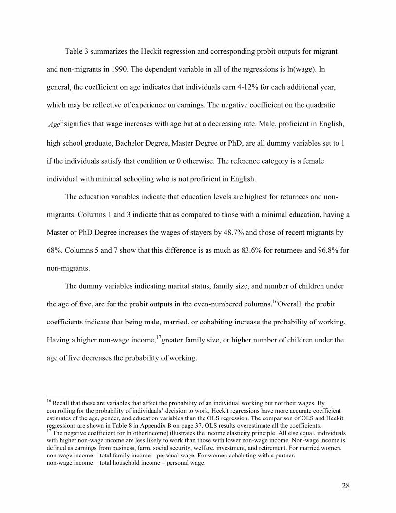
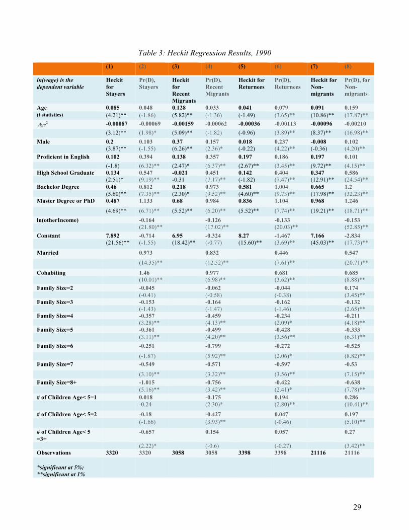
Table 3 summarizes the Heckit regression and corresponding probit outputs for migrant

and non-migrants in 1990. The dependent variable in all of the regressions is ln(wage). In

general, the coefficient on age indicates that individuals earn 4-12% for each additional year,

which may be reflective of experience on earnings. The negative coefficient on the quadratic

2Age signifies that wage increases with age but at a decreasing rate. Male, proficient in English,

high school graduate, Bachelor Degree, Master Degree or PhD, are all dummy variables set to 1

if the individuals satisfy that condition or 0 otherwise. The reference category is a female

individual with minimal schooling who is not proficient in English.

The education variables indicate that education levels are highest for returnees and non-

migrants. Columns 1 and 3 indicate that as compared to those with a minimal education, having a

Master or PhD Degree increases the wages of stayers by 48.7% and those of recent migrants by

68%. Columns 5 and 7 show that this difference is as much as 83.6% for returnees and 96.8% for

non-migrants.

The dummy variables indicating marital status, family size, and number of children under

the age of five, are for the probit outputs in the even-numbered columns.16Overall, the probit

coefficients indicate that being male, married, or cohabiting increase the probability of working.

Having a higher non-wage income,17greater family size, or higher number of children under the

age of five decreases the probability of working.

16 Recall that these are variables that affect the probability of an individual working but not their wages. By controlling for the probability of individuals’ decision to work, Heckit regressions have more accurate coefficient estimates of the age, gender, and education variables than the OLS regression. The comparison of OLS and Heckit regressions are shown in Table 8 in Appendix B on page 37. OLS results overestimate all the coefficients. 17 The negative coefficient for ln(otherIncome) illustrates the income elasticity principle. All else equal, individuals with higher non-wage income are less likely to work than those with lower non-wage income. Non-wage income is defined as earnings from business, farm, social security, welfare, investment, and retirement. For married women, non-wage income = total family income – personal wage. For women cohabiting with a partner, non-wage income = total household income – personal wage.

29

Table 3: Heckit Regression Results, 1990 (1) (2) (3) (4) (5) (6) (7) (8)

ln(wage) is the dependent variable

Heckit for Stayers

Pr(D), Stayers

Heckit for Recent Migrants

Pr(D), Recent Migrants

Heckit for Returnees

Pr(D), Returnees

Heckit for Non-migrants

Pr(D), for Non-migrants

Age 0.085 0.048 0.128 0.033 0.041 0.079 0.091 0.159 (t statistics) (4.21)** (-1.86) (5.82)** (-1.36) (-1.49) (3.65)** (10.86)** (17.87)**

2Age -0.00087 -0.00069 -0.00159 -0.00062 -0.00036 -0.00113 -0.00096 -0.00210 (3.12)** (1.98)* (5.09)** (-1.82) (-0.96) (3.89)** (8.37)** (16.98)** Male 0.2 0.103 0.37 0.157 0.018 0.237 -0.008 0.102 (3.87)** (-1.55) (6.26)** (2.36)* (-0.22) (4.22)** (-0.36) (4.20)** Proficient in English 0.102 0.394 0.138 0.357 0.197 0.186 0.197 0.101 (-1.8) (6.32)** (2.47)* (6.37)** (2.67)** (3.45)** (9.72)** (4.15)** High School Graduate 0.134 0.547 -0.021 0.451 0.142 0.404 0.347 0.586 (2.51)* (9.19)** -0.31 (7.17)** (-1.82) (7.47)** (12.91)** (24.54)** Bachelor Degree 0.46 0.812 0.218 0.973 0.581 1.004 0.665 1.2 (5.60)** (7.35)** (2.30)* (9.52)** (4.60)** (9.73)** (17.98)** (32.23)** Master Degree or PhD 0.487 1.133 0.68 0.984 0.836 1.104 0.968 1.246

(4.69)** (6.71)** (5.52)** (6.20)** (5.52)** (7.74)** (19.21)** (18.71)** ln(otherIncome) -0.164 -0.126 -0.133 -0.153 (21.80)** (17.02)** (20.03)** (52.85)** Constant 7.892 -0.714 6.95 -0.324 8.27 -1.467 7.166 -2.834 (21.56)** (-1.55) (18.42)** (-0.77) (15.60)** (3.69)** (45.03)** (17.73)**

Married 0.973 0.832 0.446 0.547

(14.35)** (12.52)** (7.61)** (20.71)**

Cohabiting 1.46 0.977 0.681 0.685 (10.01)** (6.98)** (3.62)** (8.88)** Family Size=2 -0.045 -0.062 -0.044 0.174 (-0.41) (-0.58) (-0.38) (3.45)** Family Size=3 -0.153 -0.164 -0.162 -0.132 (-1.43) (-1.47) (-1.46) (2.65)** Family Size=4 -0.357 -0.459 -0.234 -0.211 (3.28)** (4.13)** (2.09)* (4.18)** Family Size=5 -0.361 -0.499 -0.428 -0.333 (3.11)** (4.20)** (3.56)** (6.31)** Family Size=6 -0.251 -0.799 -0.272 -0.525

(-1.87) (5.92)** (2.06)* (8.82)** Family Size=7 -0.549 -0.571 -0.597 -0.53

(3.10)** (3.32)** (3.56)** (7.15)** Family Size=8+ -1.015 -0.756 -0.422 -0.638 (5.16)** (3.42)** (2.41)* (7.78)** # of Children Age< 5=1 0.018 -0.175 0.194 0.286 -0.24 (2.30)* (2.80)** (10.41)**

# of Children Age< 5=2 -0.18 -0.427 0.047 0.197 (-1.66) (3.93)** (-0.46) (5.10)**

# of Children Age< 5 =3+

-0.657 0.154 0.057 0.27

(2.22)* (-0.6) (-0.27) (3.42)** Observations 3320 3320 3058 3058 3398 3398 21116 21116 *significant at 5%; **significant at 1%

30

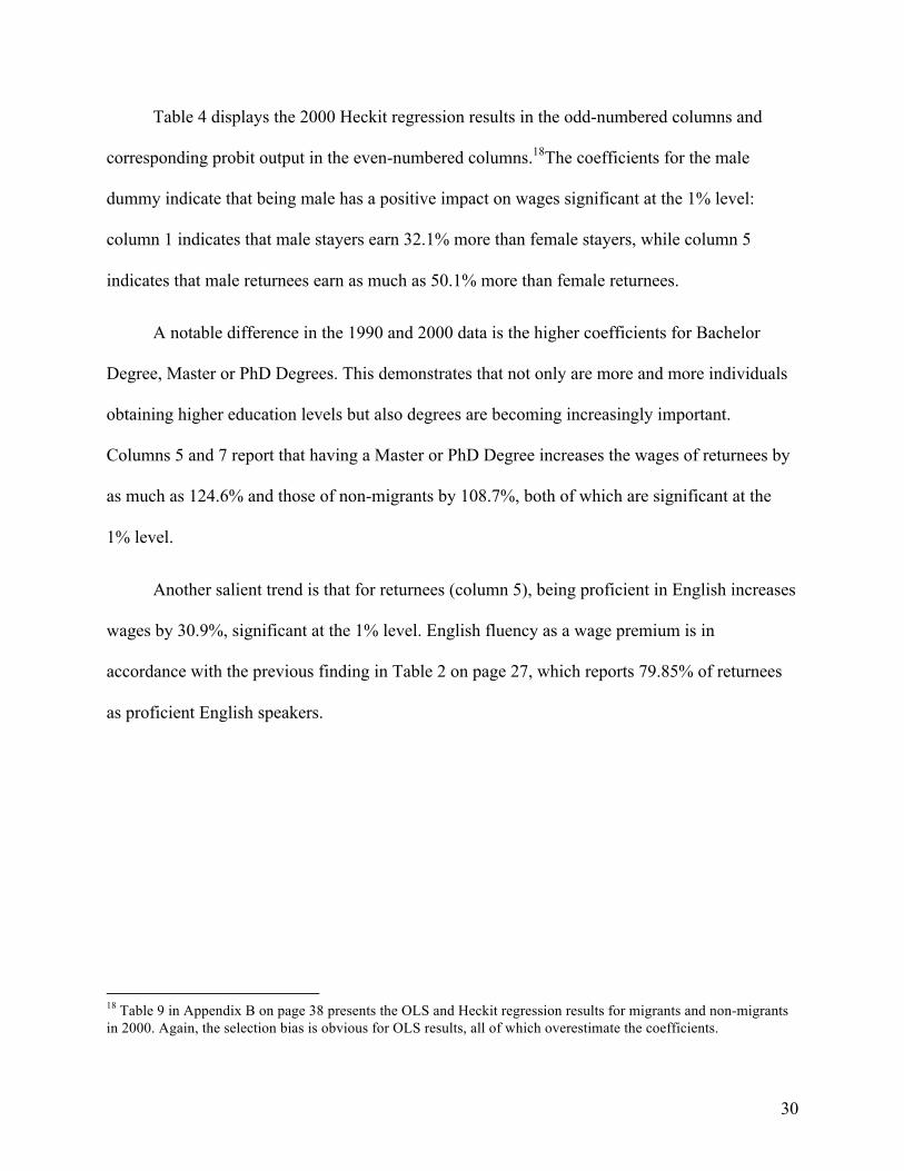
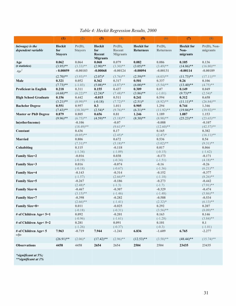
Table 4 displays the 2000 Heckit regression results in the odd-numbered columns and

corresponding probit output in the even-numbered columns.18The coefficients for the male

dummy indicate that being male has a positive impact on wages significant at the 1% level:

column 1 indicates that male stayers earn 32.1% more than female stayers, while column 5

indicates that male returnees earn as much as 50.1% more than female returnees.

A notable difference in the 1990 and 2000 data is the higher coefficients for Bachelor

Degree, Master or PhD Degrees. This demonstrates that not only are more and more individuals

obtaining higher education levels but also degrees are becoming increasingly important.

Columns 5 and 7 report that having a Master or PhD Degree increases the wages of returnees by

as much as 124.6% and those of non-migrants by 108.7%, both of which are significant at the

1% level.

Another salient trend is that for returnees (column 5), being proficient in English increases

wages by 30.9%, significant at the 1% level. English fluency as a wage premium is in

accordance with the previous finding in Table 2 on page 27, which reports 79.85% of returnees

as proficient English speakers.

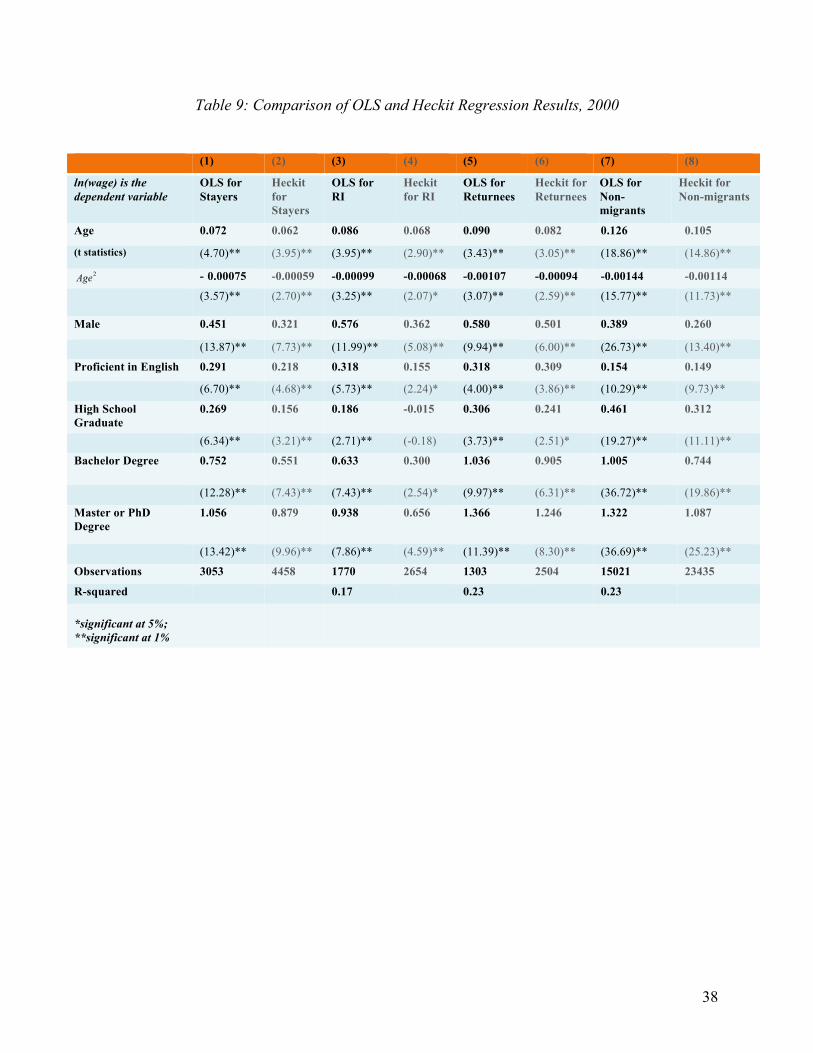
18 Table 9 in Appendix B on page 38 presents the OLS and Heckit regression results for migrants and non-migrants in 2000. Again, the selection bias is obvious for OLS results, all of which overestimate the coefficients.

31

Table 4: Heckit Regression Results, 2000 (1) (2) (3) (4) (5) (6) (7) (8)


Heckit for Stayers

Pr(D), Stayers


Pr(D), Recent Migrants


Pr(D), Returnees


Pr(D), Non-migrants

Age 0.062 0.064 0.068 0.079 0.082 0.086 0.105 0.136 (t statistics) (3.95)** (3.33)** (2.90)** (3.30)** (3.05)** (3.49)** (14.86)** (16.80)**

2Age - 0.00059 -0.00103 -0.00068 -0.00124 -0.00094 -0.00131 -0.00114 -0.00189

(2.70)** (3.93)** (2.07)* (3.76)** (2.59)** (4.03)** (11.73)** (17.11)** Male 0.321 0.052 0.362 0.317 0.501 0.337 0.26 0.106 (7.73)** (-1.03) (5.08)** (4.87)** (6.00)** (5.54)** (13.40)** (4.75)** Proficient in English 0.218 0.311 0.155 0.437 0.309 0.07 0.149 0.049 (4.68)** (6.22)** (2.24)* (7.48)** (3.86)** (-1.01) (9.73)** (2.54)* High School Graduate 0.156 0.442 -0.015 0.511 0.241 0.594 0.312 0.658 (3.21)** (8.99)** (-0.18) (7.72)** (2.51)* (8.92)** (11.11)** (26.84)** Bachelor Degree 0.551 0.957 0.3 1.011 0.905 1.294 0.744 1.346 (7.43)** (10.30)** (2.54)* (9.76)** (6.31)** (11.92)** (19.86)** (39.92)** Master or PhD Degree 0.879 0.805 0.656 0.81 1.246 1.189 1.087 1.153 (9.96)** (6.75)** (4.59)** (5.18)** (8.30)** (8.98)** (25.23)** (23.65)** ln(otherIncome) -0.106 -0.07 -0.088 -0.107 (18.49)** (9.61)** (12.60)** (42.57)** Constant 0.436 0.17 0.165 0.382 (8.05)** (2.45)* (2.47)* (16.11)** Married 0.806 0.672 0.536 0.54 (7.31)** (5.18)** (3.02)** (9.31)** Cohabiting 0.115 -0.118 0.017 0.066 (-1.34) (-1.09) (-0.15) (-1.62) Family Size=2 -0.016 0.038 -0.173 -0.171 (-0.19) (-0.34) (-1.51) (4.18)** Family Size=3 0.016 -0.074 -0.16 -0.26 (-0.18) (-0.67) (-1.36) (6.21)** Family Size=4 -0.143 -0.314 -0.152 -0.377 (-1.57) (2.66)** (-1.18) (8.26)** Family Size=5 -0.267 -0.186 -0.273 -0.442 (2.48)* (-1.3) (-1.7) (7.91)** Family Size=6 -0.467 -0.307 -0.329 -0.474 (3.15)** (-1.46) (-1.48) (5.86)** Family Size=7 -0.398 -0.282 -0.588 -0.534 (2.66)** (-1.41) (2.32)* (6.13)** Family Size=8+ 0.011 -0.025 0.292 0.207 (-0.18) (-0.31) (3.56)** (8.09)** # of Children Age< 5=1 0.092 -0.201 0.163 0.146 (-0.96) (-1.61) (-1.28) (3.84)** # of Children Age< 5=2 0.281 0.091 0.101 0.1 (-1.26) (-0.37) (-0.3) (-1.01) # of Children Age< 5 =3+

7.963 -0.719 7.944 -1.241 6.836 -1.609 6.765 -2.277

(26.91)** (2.06)* (17.42)** (2.96)** (12.53)** (3.58)** (48.44)** (15.74)**

Observations 4458 4458 2654 2654 2504 2504 23435 23435

*significant at 5%; **significant at 1%

32

VII. Conclusion

The results indicate that Puerto Rican migrants on average earn more in the U.S. than in

PR. Of the four groups in both 1990 and 2000, stayers have the highest wages. The

counterfactual predicted wages indicate that returnees and non-migrants would have earned more

had they stayed in the U.S. or migrated but their residence in PR reveals that wage differentials

are not the only consideration in individuals’ decision to migrate.

Overall, the 2000 descriptive data provide strong support for negative self-selection,

which is consistent with Borjas’s and Ramos’s expectations. This is a notable change from the

positive self-selection as indicated by 1990 data. As Ramos noted earlier, the change may be

indicative of the social and economic variations between the U.S. and PR from 1990 to 2000.

The shift in self-selection type may be due in part to changes in federal tax break laws to U.S>

companies with operations in PR and in the income inequality between the U.S. and PR.

In fact,1989 is the year in which income inequality was at its lowest in PR by the Gini19

scale. From then onward, the Gini coefficient increased such that the absolute income gap

between the poor and the rich widened and the labor market favored those with higher education

(Toro, 2008). During the same ten-year span, the U.S. income wage distribution increased as

well, although at a slower pace than in PR, indicating the potential contributing factor for the

reversal in self-selection type of Puerto Rican migrants in 1990 and 2000.

19 See footnote 4 on page 8 for an explanation of the Gini coefficient.

33

Appendix A: Figure

Figure 8: U.S. Hispanic Population (in Thousands), 1994 to 2008

The y-axis is the number of migrants in thousands. The x-axis is the year.

The green bars show the steady growth of the Hispanic population in the U.S., with the red bars-which represent the Mexican population- staying consistently above the 50% level from 1994 to 2008. Mexicans are the largest and the fastest growing migrant group. The blue bars represent the Puerto Ricans, the second largest Hispanic population in the U.S. In contrast to the steadfast increase of the Mexican population, the Puerto Rican population actually dropped by approximately 200,000 in 2005, which may be reflective of the relative social and economic conditions in the U.S. and PR. All numbers should be interpreted within the context of the freedom to cross borders, or unrestricted flow. The fact that Puerto Ricans are U.S. citizens allows them to move freely in and out of the country. Source: United States Census Bureau, Current Population Survey. http://www.census.gov/population/www/socdemo/hispanic/tables.html.

0 2500 5000 7500 10000 12500 15000 17500 20000 22500 25000 27500 30000 32500 35000 37500 40000 42500 45000 47500

1994 1995 1996 1997 1998 1999 2000 2001 2002 2003 2004 2005 2006 2007 2008

Puerto Ricans

Mexicans

Hispanic

34

Appendix B: Additional Stata Output Tables

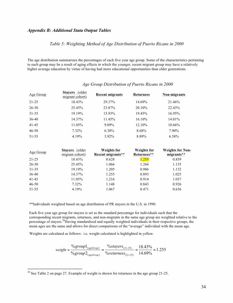
Table 5: Weighting Method of Age Distribution of Puerto Ricans in 2000

The age distribution summarizes the percentages of each five year age group. Some of the characteristics pertaining to each group may be a result of aging effects in which the younger, recent migrant group may have a relatively higher average education by virtue of having had more educational opportunities than older generations.

Age Group Distribution of Puerto Ricans in 2000

Age Group Stayers (older migrant cohort) Recent migrants Returnees Non-migrants

21-25 18.43% 29.37% 14.69% 21.46% 26-30 25.45% 23.87% 20.10% 22.43% 31-35 19.19% 15.93% 19.45% 16.95% 36-40 14.37% 11.45% 16.10% 14.01% 41-45 11.05% 9.09% 12.10% 10.66% 46-50 7.32% 6.38% 8.68% 7.90% 51-55 4.19% 3.92% 8.89% 6.58%

Age Group Stayers (older migrant cohort)

Weights for Recent migrants**

Weights for Returnees**

Weights for Non-migrants**

21-25 18.43% 0.628 1.255 0.859 26-30 25.45% 1.066 1.266 1.135 31-35 19.19% 1.205 0.986 1.132 36-40 14.37% 1.255 0.893 1.025 41-45 11.05% 1.216 0.914 1.037 46-50 7.32% 1.148 0.843 0.926 51-55 4.19% 1.067 0.471 0.636

**Individuals weighted based on age distribution of PR stayers in the U.S. in 1990. Each five year age group for stayers is set as the standard percentage for individuals such that the corresponding recent migrants, returnees, and non-migrants in the same age group are weighted relative to the percentage of stayers.20Having standardized and equally weighted individuals in their respective groups, the mean ages are the same and allows for direct comparisons of the “average” individual with the mean age.

Weights are calculated as follows: i.e. weight calculated is highlighted in yellow.

( ) (21 25)

( ) (21 25)

% 1 % 18.43% 1.255% 2 % 14.69%

ageGroup

ageGroup

weightgroup stayersgroup returnees

−

−

= = = =

20 See Table 2 on page 27. Example of weight is shown for returnees in the age group 21-25.

35

Table 6: Non-weighted Descriptive Data, 1990

Puerto Rican Migrants and Non-migrants, 1990 Censuses 1990 U.S. Census 1990 U.S. Census 1990 PR Census 1990 PR Census Groups Stayers Recent migrants Returnees Non-migrants Sample Size, Observations 3320 3058 3398 21116 Period of Residence in the U.S. 1980-1990 1986-1990 19??-1985 n/a Mean Age 33.675 32.030 35.615 33.995 Gender: % male 45.54% 44.28% 48.44% 47.42% Mean Education (av of codes 1-4) 1.820 1.953 1.742 1.931

% minimal schooling (code 1) 34.85% 26.95% 41.61% 28.66% % high school graduate (code 2) 52.44% 55.26% 46.50% 53.32% % Bachelor Degree (code 3) 8.52% 13.37% 7.98% 14.32% % Master/PhD Degree (code 4) 4.19% 4.41% 3.91% 3.71%

Mean Wage in US** (number of observations) Mean Wage for Males Mean Wage for Females

23176.30 (2053)

M: 26519.62 F: 18419.85

17957.18 (1867)

M: 20772.71 F: 14454.69

n/a*

n/a*

Mean Wage in PR** (number of observations) Mean Wage for Males Mean Wage for Females

n/a*

n/a*

15304.97 (1612)

M: 17469.61 F: 11595.20

14354.00 (12276)

M: 15566.44 F: 12642.88

Marital Status % single 40.33% 36.36% 32.52% 26.09% % married 54.40% 57.36% 65.36% 71.81% % cohabiting 5.27% 6.28% 2.12% 2.09% English Fluency % not proficient 27.02% 39.99% 32.31% 71.85% % proficient 72.98% 60.01% 67.69% 28.15% Average Number of Children at Home (0-9)

1.367 1.308 1.332 1.434

*Unobserved wages. Individuals' wages cannot be observed in both locations contemporaneously due to impossibility of having the same individuals being present in two countries at the same time. See Table 4 for predicted wages. **All wage computations standardized to 1999 dollars.

Table 6 summarizes the non-weighted descriptive data for migrant and non-migrant groups, which is interesting but not as practical as the weighted data. For a more insightful comparison, it is instructive to examine Table 1 on page 25 which has weighted all the age groups in the recent migrants, returnees, and non-migrants groups to match those of the stayers.

36

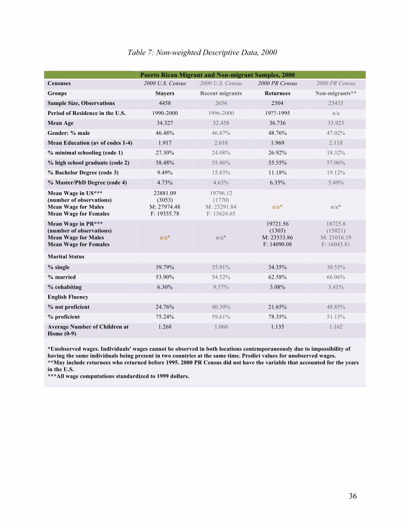
Table 7: Non-weighted Descriptive Data, 2000

Puerto Rican Migrant and Non-migrant Samples, 2000 Censuses 2000 U.S. Census 2000 U.S. Census 2000 PR Census 2000 PR Census

Groups Stayers Recent migrants Returnees Non-migrants**

Sample Size, Observations 4458 2654 2504 23435


Mean Age 34.327 32.458 36.736 33.923

Gender: % male 46.48% 46.87% 48.76% 47.02%






Mean Wage in US*** (number of observations) Mean Wage for Males Mean Wage for Females

23881.09 (3053)

M: 27974.48 F: 19355.78

19796.12 (1770)

M: 23291.84 F: 15624.65

n/a*

n/a*

Mean Wage in PR*** (number of observations) Mean Wage for Males Mean Wage for Females

n/a*

n/a*

19721.56 (1303)

M: 23533.86 F: 14090.08

18725.8 (15021)

M: 21016.19 F: 16043.81

Marital Status

% single 39.79% 35.91% 34.35% 30.53%

% married 53.90% 54.52% 62.58% 66.06%

% cohabiting 6.30% 9.57% 3.08% 3.41%

English Fluency

% not proficient 24.76% 40.39% 21.65% 48.85%

% proficient 75.24% 59.61% 78.35% 51.15%


1.268 1.060 1.135 1.162

*Unobserved wages. Individuals' wages cannot be observed in both locations contemporaneously due to impossibility of having the same individuals being present in two countries at the same time. Predict values for unobserved wages. **May include returnees who returned before 1995. 2000 PR Census did not have the variable that accounted for the years in the U.S. ***All wage computations standardized to 1999 dollars.

37

Table 8: Comparison of OLS and Heckit Regression Results, 1990

(1) (2) (3) (4) (5) (6) (7) (8) ln(wage) is the dependent variable

OLS for Stayers

Heckit for Stayers

OLS for Recent Migrants


OLS for Returnees


OLS for Non-migrants


Age 0.092 0.085 0.124 0.128 0.069 0.041 0.133 0.091 (t statistics)

(4.80)** (4.21)** (5.78)** (5.82)** (2.63)** (-1.49) (16.91)** (10.86)** 2Age - 0.00096 - 0.00087 - 0.00158 -0.00159 -0.00079 -0.00036 -0.00151 -0.00096

(3.63)** (3.12)** (5.17)** (5.09)** (2.22)* (-0.96) (14.05)** (8.37)** Male 0.533 0.200 0.588 0.370 0.455 0.018 0.299 -0.008 (13.81)** (3.87)** (12.87)** (6.26)** (7.57)** (-0.22) (17.29)** (-0.36) Proficient in English 0.264 0.102 0.252 0.138 0.307 0.197 0.222 0.197

(5.04)** (-1.80) (4.86)** (2.47)* (4.38)** (2.67)** (11.61)** (9.72)**

High School Graduate

0.347 0.134 0.125 -0.021 0.384 0.142 0.617 0.347

(7.32)** (2.51)* (1.98)* (-0.31) (5.52)** (-1.82) (26.29)** (12.91)**

Bachelor Degree 0.761 0.460 0.502 0.218 1.111 0.581 1.114 0.665

(10.62)** (5.60)** (6.26)** (2.30)* (11.06)** (4.60)** (37.77)** (17.98)** Master or PhD Degree

0.846 0.487 0.965 0.680 1.333 0.836 1.408 0.968

(9.45)** (4.69)** (8.82)** (5.52)** (10.43)** (5.52)** (32.51)** (19.21)**

Constant 6.938 7.892 6.442 6.950 6.692 8.270 5.610 7.166 (20.69)** (21.56)** (17.99)** (18.42)** (14.19)** (15.60)** (40.65)** (45.03)**

Observations 2052 3320 1867 3058 1612 3398 12276 21116 R-squared 0.19 0.18 0.16 0.23 *significant at 5%; **significant at 1%

38

Table 9: Comparison of OLS and Heckit Regression Results, 2000

(1) (2) (3) (4) (5) (6) (7) (8)


OLS for Stayers

Heckit for Stayers

OLS for RI

Heckit for RI

OLS for Returnees


OLS for Non-migrants


Age 0.072 0.062 0.086 0.068 0.090 0.082 0.126 0.105

(t statistics) (4.70)** (3.95)** (3.95)** (2.90)** (3.43)** (3.05)** (18.86)** (14.86)** 2Age - 0.00075 -0.00059 -0.00099 -0.00068 -0.00107 -0.00094 -0.00144 -0.00114

(3.57)** (2.70)** (3.25)** (2.07)* (3.07)** (2.59)** (15.77)** (11.73)**

Male 0.451 0.321 0.576 0.362 0.580 0.501 0.389 0.260

(13.87)** (7.73)** (11.99)** (5.08)** (9.94)** (6.00)** (26.73)** (13.40)**

Proficient in English 0.291 0.218 0.318 0.155 0.318 0.309 0.154 0.149

(6.70)** (4.68)** (5.73)** (2.24)* (4.00)** (3.86)** (10.29)** (9.73)**

High School Graduate

0.269 0.156 0.186 -0.015 0.306 0.241 0.461 0.312

(6.34)** (3.21)** (2.71)** (-0.18) (3.73)** (2.51)* (19.27)** (11.11)**

Bachelor Degree 0.752 0.551 0.633 0.300 1.036 0.905 1.005 0.744

(12.28)** (7.43)** (7.43)** (2.54)* (9.97)** (6.31)** (36.72)** (19.86)**

Master or PhD Degree

1.056 0.879 0.938 0.656 1.366 1.246 1.322 1.087

(13.42)** (9.96)** (7.86)** (4.59)** (11.39)** (8.30)** (36.69)** (25.23)**

Observations 3053 4458 1770 2654 1303 2504 15021 23435

R-squared 0.17 0.23 0.23 *significant at 5%; **significant at 1%

39

Bibliography

Autor, D. H. (2003, Nov 14). Lecture Note: Self-Selection – The Roy Model. Retrieved Nov 14,

2010, from MIT: http://econ-www.mit.edu/files/551

Borjas, G. J. (1999). The Economic Analysis of Immigration. Handbook of Labor Economics,

Volume 3A, pp. 1697-1760.

Borjas, G. (2008). Immigration. Retrieved Nov 23, 2010, from The Concise Encyclopedia of

Economics: http://www.econlib.org/library/Enc/Immigration.html Borjas, G. J. (2007, Dec). Labor Outflows and Labor Inflows in Puerto Rico. Retrieved Nov 1,

2010, from National Bureau of Economic Research: http://www.nber.org/papers/w13669

Borjas, G. J. (1987, Sep). Self-Selection and the Earnings of Immigrants. American Economic

Review, pp. 531-553.

Borjas, G. J., & Bratsberg, B. (1996, Feb). Who Leaves? The Outmigration of the Foreign-Born.

Review of Economics and Statistics , pp. 165-176.

Collazo, S. G., Ryan, C. L., & Bauman, K. J. (2010, April 15). Profile of the Puerto Rican

Population in United States and Puerto Rico: 2008. Retrieved Nov 24, 2010, from U.S.

Census Bureau: www.census.gov/hhes/.../Collazo_Ryan_Bauman_PAA2010_Paper.pdf

Coulon, A. d., & Piracha, M. (2005). Self-Selection and the Performance of Return Migrants: the

Source Country Perspective. Journal of Population Economics, Vol. 18, Issue 4 , pp. 779-

807.

Francis, D. R. (2007, Feb). Spreading the Gains from Immigration. The NBER Digest, pp. 4-6. Gronau, R. (1974). Wage Comparison-- A Selectivity Bias. The Journal of Political Economy,

82 (6), 1119-1143.

40

Preston, S. H., & Hartnett, C. S. (2008, Nov). The Future of American Fertility. Retrieved Dec 1,

2010, from National Bureau of Economic Research:

http://www.nber.org/papers/w14498.pdf

Projected Population of the United States, by Race and Hispanic Origin: 2000 to 2050. (2004,

March 18). Retrieved Feb 28, 2011, from U.S. Census Bureau:

http://www.census.gov/ipc/www/usinterimproj/

Ramos, F. (1992). Out-migration and Return Migration of Puerto Ricans. In G. J. Borjas, & R. B.

Freeman (eds), Immigration and the Workforce: Economic Consequences for the United

States and Source Areas (pp. 49-66). University of Chicago Press.

Toro, H. (2008). Revista Harvard Review of Latin America.

Wooldridge, J. M. (2003). Limited Dependent Variable Models and Sample Selection

Corrections. In J. M. Wooldridge, Introductory Econometrics: A Modern Approach, 2e

(pp. 579-592). United States: Thomson South-Western.

Wooldridge, J. M. (2002). Sample Selection, Attrition, and Stratified Sampling. In J. M.

Wooldridge, Econometric Analysis of Cross Section and Panel Data (pp. 560-566).

Cambridge: MIT.

welcome to the united states: self-selection of … · welcome to the united states: self-selection...

Documents