International Migration, Self-Selection, and the Distribution of Wages: Evidence from Mexico and the United States

August 2004

Daniel Chiquiar Bank of Mexico

Gordon H. Hanson

University of California, San Diego and National Bureau of Economic Research

Abstract. In this paper, we use data from the 1990 and 2000 Mexico and U.S. population censuses to examine who migrates from Mexico to the U.S. and how their skills and economic performance compare to those who remain in Mexico. We use these data to test Borjas’ (1987) negative-selection hypothesis that in countries with high returns to skill and high earnings inequality (e.g., Mexico) those most likely to migrate to countries with low returns to skill and low earnings inequality (e.g., the U.S.) are the less skilled. We find that 1) Mexican immigrants, while much less educated than U.S. natives, are on average more educated than residents of Mexico, and 2) were Mexican immigrants in the U.S. to be paid according to current skill prices in Mexico they would tend to occupy the middle and upper portions of Mexico’s wage distribution. These results are inconsistent with the negative-selection hypothesis and suggest, instead, that in terms of observable skills there is intermediate or positive selection of immigrants from Mexico. We thank Kate Antonovics, Julian Betts, Richard Carson, Gary Ramey, James Rauch, Chris Woodruff and seminar participants at American University, the Banco de Mexico, the CIA, El Colegio de Mexico, the University of Houston, the NBER, Occidental College, Stanford University, UC Berkeley, UC San Diego, the University of Toronto, and Yale University for helpful comments. The opinions in this paper correspond to the authors and do not necessarily reflect the viewpoint of the Banco de México.

1. Introduction

In recent decades, rising immigration from poor countries has made the U.S. labor

force larger, younger, and less-skilled than it otherwise would have been (Borjas, 1999).

The shift in immigrant composition appears due in part to the 1965 Immigration Act,

which relaxed long-standing country-of-origin restrictions on immigrant admissions.

In an important body of work, Borjas (1987) argues that who migrates to the U.S.

from a particular country will depend on that country’s wage distribution. In countries

with high returns to skill and high wage dispersion, as in much of the developing world,

there will be negative selection of immigrants. Those with the greatest incentive to

migrate to the U.S. will be individuals with below-average skill levels in their home

countries. In countries with low returns to skill and low wage dispersion, as appears to be

the case in Western Europe, there will be positive selection of immigrants. Those with

above-average skill levels will have the greatest incentive to migrate. In support of this

selection hypothesis, Borjas (1987, 1995) finds that as sources for U.S. immigration have

shifted from Europe to Asia and Latin America, the economic performance of new

immigrants has deteriorated. Relative to earlier cohorts, recent immigrants earn lower

wages compared to natives at time of arrival and take longer for their earnings to

converge to native levels.1 These findings counter an earlier belief that, irrespective of

origin country, immigrants have high potential for earnings growth (Chiswick, 1978).2

Largely missing in the discussion of U.S. immigration is evidence from source

countries. Surprisingly, there is little work on how the skills of immigrants compare to

1 Identifying changes in the average quality of immigrant cohorts is complicated by changes in unobserved cohort quality, immigrant assimilation, and labor-market disturbances that vary by skill group. See LaLonde and Topel (1992, 1997), Borjas (1999) and Butcher and DiNardo (2002) on how to deal with this issue. 2 Evidence of positive selection includes brain drain from poor countries (Beine et al., 2001; Carrington et al., 1998) and the internal migration of skilled workers (Borjas, Bronars, and Trejo, 1992; Bound and Holzer, 2000).

1

the skills of non-migrating individuals in countries of origin. Such data are essential to

evaluate the nature of migrant selection. One exception is Ramos (1992) who uses 1980

census data for the U.S. and Puerto Rico. Consistent with negative selection, non-

migrants in Puerto Rico are more educated than individuals migrating from Puerto Rico

to the U.S. and less educated than those migrating from the U.S. to Puerto Rico.3

In this paper, we use data from the 1990 and 2000 Mexico population censuses

and data on Mexican immigrants in the 1990 and 2000 U.S. population censuses to

examine who in Mexico migrates to the U.S. and how their earnings and observable skills

compare to those who remain at home. Mexico is the largest source country for U.S.

immigration, accounting for 31.3% of net new arrivals in the 1990’s. In 2000 the 9.2

million Mexican immigrants in the U.S. were equal to 9.4% of Mexico’s total population.

Mishra (2003) estimates that over the period 1970-2000 emigration raised average wages

in Mexico by 8.0%.4 Relative to the U.S., Mexico has high returns to schooling and high

wage dispersion, making it an ideal candidate to test the negative-selection hypothesis.

Following Borjas (1991), we develop a simple model, presented in section 2, to

show that migrant selection in a country like Mexico may be negative, intermediate, or

positive, depending on the size of migration costs and how they vary with skill. A simple

test for negative selection is to compare the observable skills of those who migrate and of

those who do not. In section 3, we find that Mexican immigrants, while much less

educated than U.S. natives, are more educated than residents of Mexico. Individuals with

3 To compare Ramos’ results to ours, it is important to note that many costs of migrating to the U.S. that are relevant for Mexico (binding quotas, border enforcement, bureaucratic delays) are not relevant for Puerto Rico. 4 In the U.S., many studies find that regional immigration inflows are only weakly correlated with wage changes for low-skilled U.S. natives, suggesting immigration has little impact on U.S. wages (LaLonde and Topel, 1997; Smith and Edmonston, 1997; Borjas, 1999). However, Borjas, Freeman, and Katz (1997) and Borjas (2003) argue that commonly used cross-area wage regressions require strong and unrealistic identifying assumptions. Using alternative approaches, these two studies find that higher immigration depresses wages for low-skilled U.S. natives.

2

10 to 15 years of schooling are the Mexican cohort most over-represented in the U.S.5

This is suggestive evidence against the negative selection of Mexican immigrants in

terms of observable skill.6 However, schooling may not be a sufficient statistic for skill

or for potential earnings. To compare migrants and non-migrants, we would prefer to see

what each would earn in the same labor market, under a common price for skill.

Realized earnings of non-migrants, which reflect Mexican skill prices, and of migrants,

which reflect U.S. skill prices, are not very informative.

To evaluate the selection of Mexican immigrants in terms of observable skills, we

compare actual wage densities for residents of Mexico with counterfactual wage densities

that would obtain were Mexican immigrants paid according to skill prices in Mexico.

The difference between these actual and counterfactual wage densities nonparametrically

summarizes immigrant selection in terms of potential earnings. To construct these

densities, we extend the framework in DiNardo, Fortin, and Lemieux (1996), as shown in

section 4. The results, presented in section 5, suggest that were Mexican immigrants in

the U.S. paid according to Mexican skills prices they would fall disproportionately in the

middle and upper portions of Mexico’s wage distribution. These findings do not support

negative selection and suggest instead there is intermediate or positive selection of

Mexican immigrants. Also in section 5, we examine the robustness of these results.

2. Theory

In this section, we motivate the empirical analysis by developing a simple model

of migration. Borjas (1987) applies Roy (1951) to show that in countries with relatively

5 In related work, Feliciano (2001) finds that before 1990 average schooling was also higher for Mexican immigrants. 6 Case-study evidence supports this view. See Orrenius et al. (2004), Durand et al. (2001) and Cornelius et al. (2001).

3

high returns to skill and earnings inequality migrants tend to be negatively selected – they

are drawn primarily from the lower half of the skill distribution in their home country.

Borjas (1991) shows that this result depends on assuming migration costs are constant

across individuals. If migration costs are negatively correlated with earnings, negative

selection may be overturned. We apply this insight to show that if migration costs are

decreasing in skill migrants may be negatively or positively selected in terms of skill,

depending on the size of migration costs and the shape of the skill distribution.

Individuals from Mexico, indexed by 0, choose whether or not to migrate to the

U.S., indexed by 1. For simplicity, we treat this as a one-time decision, though the

extension to a dynamic setting is straightforward (see Sjaastad, 1962; Borjas, 1991).

Residents of Mexico face a wage equation given by

sw 000 )ln( δµ += (1)

where for Mexico w0 is the wage, 0µ is the base wage, s is the level of schooling, and 0δ

is the return to schooling. We focus on migrant selection in terms of observable skills, in

this case schooling. Implicitly, we imagine there are random components to wage

determination, but for simplicity we leave such features in the background. If the

population of Mexicans were to migrate to the U.S., they would face the wage equation

sw 111)ln( δµ += (2)

where for Mexican migrants in the U.S. w1 is the wage, 1µ is the base wage, and 1δ is

the return to schooling. Consistent with skill being scarce in Mexico, we assume that

10 δδ > , or that the return to schooling is higher in Mexico than in the U.S.

Let C be migration costs and let 0w/C=π be migration costs in time-equivalent

4

units (i.e., the number of labor hours needed to migrate to the U.S.). Combining (1) and

(2), a resident of Mexico will migrate to the U.S. if

0)ln()ln()ln()ln( 0101 >−−≈+− πwwCww . (3)

Borjas (1987, 1999) assumes that π is constant, implying that all individuals require the

same number of labor hours in order to migrate to the U.S. This assumption simplifies

the analysis, but may not be an accurate reflection of reality. We assume instead that

time-equivalent migration costs decrease with schooling, such that

sππ δµπ −=)ln( . (4)

This corresponds to the case in Borjas (1991), in which the random component of

earnings is negatively correlated with the random component in migration costs. Why

might migration costs decrease with schooling? First, individuals migrating legally to the

U.S. must satisfy many bureaucratic requirements, involving extensive paperwork and

repeated interactions with U.S. immigration authorities. More-educated individuals may

be able to meet these requirements more easily.7 Second, a large service industry of

lawyers and other specialists exists to help migrants manage the U.S. admissions process.

Given the cost of these services is more or less fixed, the time-equivalent cost of

migration will be lower for individuals with higher hourly wages. There is also a large

service industry oriented towards illegal immigrants (Orrenius, 1999). To enter the U.S.

successfully, an illegal entrant must cross the border, find transport to a safe location in

the U.S., and obtain counterfeit residency documents. These costs are also fixed,

implying higher-wage individuals require fewer effective labor hours to migrate to the

7 Over 90% of legal Mexicans immigrants in the U.S. are admitted under family reunification provisions of U.S. immigration law. While obtaining legal assistance cannot change an individual’s eligibility for admission, it may help an individual clear the queue for legal admission more quickly.

5

U.S. Third, credit constraints may raise migration costs for low-income individuals, who

are also likely to be less educated. Individuals may have to borrow to cover migration

costs. If lower-income individuals face higher borrowing costs, due to a higher expected

probability of default, they will face higher migration costs.8

Combining (3) and (4), Figure 1 shows and )wln( 0 π−)wln( 1 , which defines

the cutoff schooling level for who migrates to the U.S. in the case where 0=πδ and

. Here, time-equivalent migration costs are constant and small, which

corresponds to the assumptions in Borjas (1987). He focuses on unobservable skills but

the analogy to observable skills is straightforward. In Figure 1, there is negative selection

of migrants: individuals with schooling less than s

πµµµ e01 >−

* migrate from Mexico to the U.S. and

individuals with schooling greater than s* remain in Mexico. Individuals with relatively

high levels of schooling are less likely to migrate to the U.S. due to the fact that the return

to schooling in higher in Mexico.

Figure 2 shows an alternative case in which 0>πδ and .πµµµ e01 <− 9 Here,

time-equivalent migration costs are decreasing in schooling and are large. Individuals

with schooling in the interval (sL, sU) migrate from Mexico to the U.S. and those with

schooling outside this interval remain in Mexico. The selection of migrants in terms of

observable skills depends on the distribution of schooling in Mexico. There are three

possible cases: (a) negative selection: if the support for the schooling distribution goes

from some value between sL and sU to some value greater than sU, migrants will have low

8 A related possibility is that more-educated individuals may face less uncertainty with regards to the U.S. wages they would earn, making them more likely to migrate for any given wage differential.

6

schooling relative to those who remain in Mexico; (b) positive selection: if the support of

the schooling distribution runs from some value below sL to some value between sL and

sU, migrants will have relatively high levels of schooling; or (c) intermediate selection: if

the support of the schooling distribution goes from some value below sL to some value

above sU, migrants will have intermediate levels of schooling. In case (c), fixed

migration costs preclude those with low schooling from migrating and high returns to

schooling in Mexico dissuade those with high schooling from migrating, giving those

with intermediate schooling the strongest incentive to migrate to the U.S.

One caveat is that our analysis ignores migration networks, which appear to be

important in Mexico (Munshi, 2003; Woodruff and Zenteno, 2001). Individuals with

friends or relatives in the U.S. may face lower migration costs. A second caveat is that

we ignore unobservable skills. If the correlation between observable and unobservable

skills is positive and strong, we expect our results would apply to migrant selection in

terms of unobservable skills, as well. In the empirical analysis, we discuss how

migration networks and unobserved determinants of migration might affect our results.

3. Data and Preliminary Evidence

To compare outcomes for residents of Mexico and immigrants from Mexico, we

use 1% samples from Mexico’s 1990 and 2000 Census of Population and Housing and

the 5% Public Use Microdata Sample from the U.S. 1990 and 2000 Census of Population

and Housing. For much of the analysis, we focus on recent Mexican immigrants, defined

as those arriving in the U.S. within the last 10 years. They reflect individuals admitted

πµµµ e01 >−9 If (migration costs are small), then even if migration costs are decreasing in schooling there is still

an unambiguous prediction for the negative selection of migrants. An additional assumption needed to obtain Figure 2

7

under current U.S. policy. One measurement issue is that many Mexican immigrants are

in the U.S. illegally. The U.S. census shows 4.3 million Mexican-born individuals in the

U.S. in 1990 and 9.2 million in 2000. Of these, the Census Bureau estimates 1.0 million

were illegal immigrants in 1990 and 3.9 million were in 2000 (Costanzo et al., 2001). By

its own estimation, the Census Bureau undercounts illegal immigrants by 15-20%.

Others suggest the undercount rate is higher. The Immigration and Naturalization

Service (2003) puts the number of illegal Mexicans at 2.0 million in 1990 and 4.8 million

in 2000, close to estimates by Bean et al. (2001) and Passel et al. (2004).10 In section 5

we assess how undercounting illegal immigrants may affect our results.

3.1 Summary Data

Overall, the accumulated outflows of individuals born in Mexico are large. Table

1 shows Mexican immigrants in the U.S. as a percentage of the total population born in

Mexico by age cohort for males and females. We take the total Mexico-born population

to be the sum of the Mexico-born population in Mexico and the Mexico-born population

in the U.S. Consider first the cohort of males born in Mexico who were 16-25 years old

in 1990 (and thus 26-35 years old in 2000). The fraction of this cohort residing in the

U.S. was 7.6% in 1990 and 17.5% in 2000, implying that during the 1990’s about 10% of

the cohort migrated to the U.S. Consider next the cohort of males who were 26-35 years

old in 1990. The fraction of this cohort residing in the U.S. rose from 10.9% in 1990 to

15.5% in 2000, implying a within-decade emigration rate of about 4.6%. Within-decade

0

s11 es/)w(ln δ>δ+δ=∂π− ππ δ−µ

πis that ∂ for small s. 10 Most estimates of the illegal immigrant population subtract from the enumerated immigrant population new legal immigrant admissions (less estimated departures and deaths for these individuals). This residual foreign born population is taken to be illegal immigrants. See Bean et al. (2001), Costanzo et al. (2001), and INS (2003).

8

migration rates decline for each succeeding cohort. This suggests migration rates from

Mexico to the U.S. are highest for young adults. Comparing the stock of individuals in

the U.S. for different cohorts at the same age suggests that migration rates are rising over

time. The share of males 16-25 years old who resided in the U.S. rose from 7.6% in 1990

to 12.0% in 2000, and rose also for every other age group. For women migration rates

and migrant stocks are lower, but patterns are similar.

Tables 2a-2d show means for age, schooling, labor-force participation, and hourly

wages for residents of Mexico, Mexican immigrants in the U.S., and, for comparison,

other U.S. immigrants and U.S. natives. We choose education categories that are

reported in the U.S. census (Mexico reports more categories). Fortunately, these

categories correspond to modes for high grade of schooling completed in Mexico, which

occur at grade 6 (primary schooling), grade 9 (secondary schooling), and grade 12

(preparatory schooling).11 Grogger and Trejo (2002) report that Mexican immigrants

who arrive in the U.S. before age 6 complete as much education as second-generation

Mexican-Americans. In contrast, those who arrive after age 15 complete much less

schooling. To focus on migrants likely to have been schooled in Mexico, we limit the

immigrant sample to individuals aged 21 or older at time of U.S. entry.

Tables 2a-2d reproduce the familiar facts that when compared to U.S. natives

Mexican immigrants in the U.S. are younger, are much less educated, and have much

lower hourly wages. In 1990, 68.3% of all Mexican immigrant men and 62.8% of recent

11 For Mexico, average hourly wages are calculated as monthly labor income/(4.5*hours worked last week); for the U.S., average hourly wages are calculated as annual labor income/(weeks worked last year*usual hours worked per week). For Mexico, we need to assume individuals work all weeks of a month, which could bias wage estimates downwards. However, this does not affect the results in section 5 since in no exercise do we compare Mexico and U.S. wage levels. To avoid measurement error associated with implausibly low wage values or with top coding of earnings, we restrict the sample to be individuals with hourly wages between $0.05 and $20 in Mexico and $1 and $100 in the U.S. (in 1990 dollars). This restriction is nearly identical to dropping the largest and smallest 0.5% of wage values.

9

Mexican immigrant men had completed 9 or fewer years of school, compared to only

7.3% of U.S. native men. However, Mexican immigrants, and recent immigrants in

particular, compare favorably when we examine residents of Mexico. In 1990, 75.2% of

male residents of Mexico had 9 or fewer years of schooling. Beyond 9 years of

education, Mexican immigrants outperform Mexican residents in every category except

college graduates. Relative to male residents of Mexico, recent Mexican immigrant men

are less likely to have 9 or fewer years of education (62.8% versus 75.2%), more likely to

have 10-15 years of education (32.4% versus 16.3%), and less likely to have 16 plus

years of education (4.8% versus 8.4%). A similar pattern holds for women.

Over time, educational attainment among the Mexico-born has increased, but this

has not changed the gap in educational attainment between Mexican residents and

Mexican immigrants. In 2000, relative to male residents of Mexico, recent Mexican

immigrant men remain less likely to have 9 or fewer years of education (55.8% versus

69.4%), more likely to have 10-15 years (38.8% versus 19.3%), and less likely to have 16

plus years (5.4% versus 11.3%). Again, a similar pattern holds for women.

Tables 2a-2d give preliminary evidence against the negative-selection hypothesis.

In terms of observable skills, it is the moderately well educated, not the least educated,

who are most likely to migrate from Mexico to the U.S. One concern about this evidence

is that recent Mexican immigrants may have high levels of schooling in part because they

are relatively young and educational attainment in Mexico has been rising over time. To

control for age, Table 3 shows average schooling for 26-35 year old Mexican residents

and Mexican immigrants in the U.S. For this high-migration age cohort, it remains the

case that Mexican immigrants have high schooling relative to Mexican residents.

10

A related concern is that Mexican immigrants may obtain schooling after arriving

in the U.S., in which case the U.S. census would overstate educational attainment of

Mexican immigrants at the time they left Mexico. Additional schooling may take the

form of degree-oriented learning, or, more commonly, English language classes. We

have dealt with this issue in part by restricting the sample to those who were age 21 years

or older at time of arrival in the U.S. Adults appear less likely to continue schooling in

the U.S. Some adult immigrants may further their education by satisfying a high-school

equivalency requirement through passing the General Education Development (GED)

exam.12 The bunching of Mexican immigrants at exactly 12 years of education (relative

to Mexican residents) in Tables 2a-2d could be consistent with such behavior.

Available evidence indicates few Mexican immigrants pass the GED. Using the

CPS, Clark and Jaeger (2002) find that among Mexican immigrants who lack a high-

school diploma and who completed their schooling abroad only 1.2% had passed the

GED. And among Mexican immigrants who completed some schooling in the U.S. (most

of whom arrived in the U.S. as young children) only 3.7% had passed the GED. More

generally, while Betts and Lofstrom (1998) find that school enrollment rates for adult

immigrants are higher than for adult U.S. natives, the same does not hold for immigrants

from Mexico (Borjas, 1996; Trejo, 1997). Table 3 shows schooling levels for 26-35

year-old Mexican immigrants who have been in the U.S. 0-3 years or 4+ years. In 1990

and 2000, earlier arrivals are not less likely to have 12 years of schooling, suggesting

adult immigrants are unlikely to continue formal education after arriving in the U.S.

12 On the returns to a GED, see Grogger and Trejo (2002), Clark and Jaeger (2002), Cameron and Heckman (1993), and Murnane, Willett, and Tyler (2000).

11

3.2 Labor-Force Participation in Mexico and the United States

Returning to Tables 2a and 2b, there appear to be differences in labor-force

participation rates between residents of Mexico and Mexican immigrants in the U.S.

Table 4 reports the fraction of the population of Mexican residents and of recent Mexican

immigrants in the U.S. with positive labor earnings by year, age, and schooling cells.

This definition of labor-force participation reflects the sample of individuals for whom

we have observations on wages. For males 26-55 years of age with more than four years

of education, labor-force participation rates in the two countries are similar. Participation

rates are somewhat higher for Mexican immigrant males in the oldest cohort (56-65

years), and in the cohort with least schooling (0-4 years).

However, labor-force participation rates for women differ markedly between

migrants and non-migrants. Among women with 11 or fewer years of education,

immigrants are much more likely to have positive labor earnings. This could be due to

more elastic female labor supply, in which case higher wages in the U.S. would induce

higher rates of labor-force participation. Alternatively, women who are more likely to

work at any wage level may be more likely to self-select into migration. In either case,

Mexican immigrant women in the U.S. who work may differ from the subpopulation of

these women that would work were they to return to Mexico.13

This poses a problem for the empirical analysis. Differences in labor–force

participation between migrant and non-migrant females may affect the pattern of migrant

selection we uncover from data on wage earners. We return to this issue in section 4.

13 See Baker and Benjamin (1997) for further discussion of immigrant male and female labor supply.

12

3.3 Returns to Observable Skill in Mexico and the United States

A primary motivation for individuals in Mexico to emigrate is to earn higher

wages. The model in section 2 assumes that the base wage (the wage of an individual

with minimal skill) is higher in the U.S. and that returns to skill are higher in Mexico.

Available evidence is consistent with these assumptions. For Mexican immigrants in the

U.S., estimated returns to education are low. In the 1980’s and 1990’s, an additional year

of schooling is associated with an increase in log wages for men of 0.025 to 0.032

(Borjas, 1996; Trejo, 1997; Groger and Trejo, 2002).14 In Mexico in the 1990’s, an

additional year of schooling is associated with an increase in log wages for men of 0.076

to 0.097 (Chiquiar, 2003).15 Figure 3 shows kernel density estimates for wages of

Mexican immigrants and Mexican residents (individuals 21-65 years of age, where

immigrants were at least 21 years of age at time of U.S. entry and immigrated within the

previous 10 years). Not surprisingly, mean wages in Mexico are much lower.16

To summarize differences in returns to observable skills in the two countries, we

estimate OLS wage regressions for four samples of men: residents of Mexico, recent

Mexican immigrants in the U.S. (those arriving in the last 10 years), all Mexican

immigrants in the U.S., and other U.S. immigrants. Table 5 reports the results.

Unreported results for women are similar. The regressors are dummy variables for

schooling, age group, marital status, residence in a metro area, region of residence, race

(for other U.S. immigrants only), and year of entry into the U.S. (for immigrants only).

14 Bratsberg and Ragan (2002) estimate slightly higher returns to schooling (0.035) for a sample of U.S. immigrant men from any country. In all samples, the estimated return to education for U.S. natives is roughly twice as large. 15 On the returns to education in Mexico, see also Cragg and Epelbaum (1996) and Ariola and Juhn (2003). 16 Figure 3 suggests wage dispersion is lower among Mexican immigrants in the U.S. than among residents of Mexico. However, since immigrants tend to be more homogeneous than the population from which they came, it is natural for them to exhibit lower wage dispersion. This is a direct implication of self-selection (Heckman and Honore, 1990).

13

Estimated returns to schooling for residents of Mexico are much higher than for

Mexican immigrants.17 In 2000, completing 12 years of schooling is associated with an

increase in hourly wages of 60.5 log points for men in Mexico but only 11.2 to 15.4 log

points for Mexican men in the U.S. The difference is even larger for the 13-15 years and

16+ years of education categories. Returns to age are also higher for Mexican residents

than for Mexican immigrants. Table 5 confirms previous results that estimated U.S.

returns to education are lower for recent immigrants relative to earlier immigrants and for

Mexican immigrants relative to other immigrants (Borjas, 1996 and 1999).

3.4 Migration Networks, Internal Migration, and Return Migration

Unobserved characteristics surely matter for the migration decision. Individuals

may be more likely to migrate if they are highly motivated, have family or other contacts

in the U.S., or have access to credit or financial resources. In the census, information on

these features is lacking. If unobservables relevant to migration are correlated with

schooling, the evidence in Table 2 might be misleading. To gain insight into how un-

observables affect migration, we examine three groups of Mexican residents: individuals

from high-migration states, internal migrants, and return migrants from the U.S.

One important unobserved characteristic is access to migration networks. In

Mexico, there is strong historical persistence in regional migration behavior, which

suggests migration networks are regionally concentrated. This appears due in part to

historical accident. In the early 1900’s, Texas farmers began to recruit laborers in

17 If unobserved ability and schooling are correlated, estimates of returns to schooling may be biased. Also, self-selection into the labor force or into migration may introduce further biases. In unreported results, we estimated wage regressions for Mexican-born men in Mexico and in the U.S., including the inverse Mills ratio derived from a probit model of the migration decision. Since we lack an instrument for migration, identification is achieved through the non-

14

Mexico. Given then small populations on the Texas-Mexico border, recruiters followed

the main rail line into Mexico, which ran southwest to Guadalajara, a major city in the

center-west of the country. Early migrants came from rural areas near the rail line. They

helped later generations of migrants find jobs in the U.S. (Durand, Massey, and Zenteno,

2001). Emigration continues to be concentrated in central and western Mexico. The

correlation between the fractions of the Mexican state population migrating to the U.S. in

the 1950’s and in the 1990’s is 0.73 (Woodruff and Zenteno, 2001). This suggests

individuals in high-migration regions in Mexico may be the relevant comparison group

for Mexican immigrants in the U.S. Table 3 shows educational attainment for individuals

in Mexico’s high-migration states.18 Average schooling levels in these states are below

those in the rest of country, indicating that comparing Mexican immigrants with residents

of high-migration states would yield stronger evidence against negative selection.

Other important unobserved characteristics are drive and motivation, which may

help an individual take the risk of moving abroad. Similar to emigrants, internal migrants

have made the decision to relocate. Part of what distinguishes internal and external

migration is the much higher cost of migrating abroad. If it is unobserved drive, and not

migration costs, that shapes migration decisions, external and internal migrants should

have similar characteristics. Comparing Tables 2 and 3, internal migrants (adults who

resided in a different state five years previously) are more educated than Mexican

residents overall. However, relative to immigrants in the U.S. internal migrants are

under-represented among those with 10-15 years of schooling and over-represented

linear way in which the other regressors enter into the inverse Mills ratio and so depends on distributional assumptions. With these concerns in mind, correcting for self-selection into migration has little effect on the coefficient estimates. 18 These states are Aguascalientes, Colima, Guerrero, Hidalgo, Jalisco, Guanajuato, Michoacán, Morelos, Nayarít, Oaxaca, Queretero, San Luis Potosí, and Zacatecas. In 2000, 9.0% of the households in these states had sent migrants to the U.S. between 1995 and 2000, as compared to 2.6% of households in the rest of the country.

15

among those with lower and higher schooling levels. This again suggests that external

migrants are intermediately selected in terms of educational attainment.

Return migrants are individuals who have chosen not to reside in the U.S.

permanently. This may be by design – in migrating to the U.S. their plan may have been

to stay temporarily – or a result of their U.S. earnings being lower than expected. Borjas

and Bratsberg (1996) show that where migrants are positively (negatively) selected,

return migrants will be more (less) skilled than non-migrants but less (more) skilled than

permanent migrants. The Mexican census asks whether an individual resided in the U.S.

five years ago, which gives some information on the return migrant population. In Table

3, returnee women fit the pattern of positive selection (they have schooling levels

between those of residents and U.S. immigrants) but men fit neither pattern (they have

lower schooling levels than either residents or U.S. immigrants). However, extremely

small sample sizes for returnees make these results difficult to interpret.19

4. Migration Abroad and the Distribution of Wages in Mexico

In this section, we develop a framework to compare wage distributions for

residents of Mexico and immigrants from Mexico in the U.S. This exercise will allow us

to assess nonparametrically whether in terms of observable skills there is positive or

negative selection of individuals who migrate from Mexico to the U.S.

Wage distributions for Mexican residents and Mexican immigrants may differ

either because of differences in the distribution of skills between the two groups or

because of differences in the prices of skills in the two labor markets. To examine

19 The fraction of adults aged 21-64 years who reported living in the U.S. five years prior in 2000 was only 0.7% for males and 0.3% for females and in 1990 was only 0.2% for males and 0.1% for females.

16

differences in the distribution of skills between Mexican residents and Mexican

immigrants, we compute the counterfactual wage density of Mexican immigrants in the

U.S., assuming they are paid according to Mexico’s wage structure, and compare it to the

actual distribution of wages in Mexico. Our framework does not address how the

distribution of unobserved characteristics might influence the distribution of wages. If,

holding age, education, and other observables constant, Mexican immigrants in the U.S.

have low unobserved ability relative to residents of Mexico, we will tend to understate

the extent of negative selection. By taking skill prices as given, our framework also fails

to address the general-equilibrium effects of Mexico-to-U.S. migration.

4.1 Counterfactual Wage Densities

Let f i(w|x) be the density of wages w in country i, conditional on a set of

observed characteristics x. Also, let Di be an indicator variable equal to 1 if the

individual is in the labor force and equal to zero otherwise. We further define

h(x|i=Mex,Di=1) as the density of observed characteristics among wage earners in

Mexico, and h(x|i=US,Di=1) as the density of observed characteristics among wage-

earning Mexican immigrants in the U.S. To begin, we suppress time subscripts. The

observed density of wages for individuals working in Mexico is

∫ ===== dxDMexixhxwfDMexiwg iMex

i )1,|()|()1,|( (5)

Likewise, the observed density of wages for Mexicans working in the U.S. is

∫ ===== dxDUSixhxwfDUSiwg iUS

i )1,|()|()1,|( (6)

Differences in and capture differences in skill prices in the two )|( xwf Mex )|( xwf US

17

countries.20 Differences in h(x|i=Mex,Di=1) and h(x|i=US,Di=1) capture differences in

the distribution of observed characteristics for Mexican resident workers and for Mexican

immigrant workers. The differences in the h(·) functions are due in part to differences in

the characteristics of Mexican immigrants and Mexican residents and in part to

differences in who participates in the labor force in the two countries.

Consider the density of wages that would prevail for Mexican immigrant workers

in the U.S. if they were paid according to the price of skills in Mexico:

∫ === dxDUSixhxwfwg iMexMex

US )1,|()|()( (7)

This corresponds to the distribution of wages for Mexican residents in (5), except that it

is integrated over the skill distribution for working Mexican immigrants in the U.S.

While this distribution is unobserved, we can rewrite it as

dxDMexixhxwf

dxDMexixhDMexixh

DUSixhxwfwg

iMex

i

ii

MexMexUS

)1,|()|(

)1,|()1,|(

)1,|()|()(

===

====

===

∫

∫θ

(8)

where

)1,|(

)1,|(====

=i

i

DMexixhDUSixh

θ (9)

DiNardo, Fortin, and Lemieux (1996) (henceforth DFL) show that a

counterfactual density as in (7) can be estimated by taking an observed density (e.g., for

wage earners in Mexico) and re-weighting it (e.g., to reflect characteristics of Mexican

immigrant workers) as in (8). To compute the weights, use Bayes’ Law to write,

)|1,Pr()1,Pr()1,|()(

xDUSiDUSiDUSixhxh

i

ii

======

= (10)

20 When the conditional expectation is linear in the observed characteristics, these terms are closely related to the

18

and,

)|1,Pr()1,Pr()1,|()(

xDMexiDMexiDMexixhxh

i

ii

======

= (11)

Combining (10) and (11) we can obtain an expression for θ that is a function of the ratio

of the conditional probability that a Mexican-born individual works in Mexico to the

conditional probability that a Mexican-born individual works in the U.S. DFL suggest

estimating these probabilities parametrically, using the estimates to calculate θ , and then

applying the θ ’s to estimate a counterfactual wage density as in (8).

However, the counterfactual density in (8) is not precisely what we desire. The

weight, θ , as seen in (9), adjusts for differences in the distribution of skills between

Mexican immigrants and Mexican residents, conditional on Mexican immigrants working

in the U.S. and Mexican residents working in Mexico. In order to compare wage

distributions for the two groups, we want to condition on common labor-force

participation behavior, which requires modifying the weight we use to construct the

counterfactual wage density. First, note that it is possible to write the joint probability of

migration and labor-force participation, conditional on x, as the product of the conditional

distribution of the participation outcome and the marginal of the migration outcome:

)|Pr(),|1Pr()|1,Pr( xUSixUSiDxDUSi ii ====== (12)

)|Pr(),|1Pr()|1,Pr( xMexixMexiDxDMexi ii ====== (13)

Given (9)-(13), we can write:

)1,Pr()|Pr(),|1Pr()1,Pr()|Pr(),|1Pr(

==========

=ii

ii

DUSixMexixMexiDDMexixUSixUSiD

θ (14)

regression equation for wages on observable characteristics (Butcher and DiNardo, 2002).

19

Next, note that Pr(i = Mex, Di=1)/Pr(i = US, Di=1) is a constant given by the

sample proportions of Mexican resident and Mexican immigrant workers. Since θ is

scaled to sum to one once we estimate wage densities, we can without loss of generality

set Pr(i = Mex, Di=1)/Pr(i = US, Di=1) = 1. Thus, the weight θ can be written as,

(15) MPθθθ =

where:

⎟⎟⎠

⎞⎜⎜⎝

⎛====

=),|1Pr(

),|1Pr(xMexiD

xUSiD

i

iPθ and ⎟⎟⎠

⎞⎜⎜⎝

⎛==

=)|Pr(

)|Pr(xMexi

xUSiMθ (16)

The first ratio – the conditional probability of a Mexican immigrant in the U.S. working

over the conditional probability of a Mexican resident working – adjusts Mexico’s wage

density in (8) to reflect U.S. labor-force participation rates for each realization of x. The

second ratio – the probability of a Mexican-born individual being in the U.S. over the

probability of a Mexican-born individual being in Mexico – adjusts the wage density of

Mexican residents to reflect the characteristics of Mexican immigrants.

The second ratio, , is the appropriate weight to construct counterfactual wage

densities. The full weight,

Mθ

θ , adjusts for differences in observables and in labor-force

participation between Mexican immigrants and residents. In (8), we replace θ with ,

which yields the wage distribution that would obtain if immigrants were paid according

to Mexican skill prices and participated in the labor force as do Mexican residents.

Mθ

21

To compute , we estimate Pr(i=US | x) parametrically by running a logit on

the probability of a Mexican adult being in the U.S. using the full sample of Mexican

Mθ

21 For males, θ and are close in value (male labor-force participation is similar in the two countries), and either weight yields similar results. For females, labor-force participation rates differ in the two countries (see Table 4). The

Mθ

20

immigrants and Mexican residents (and not just wage earners). Once we estimate this

model, we can compute Pr(i=Mex | x) = 1 - Pr(i=US | x) and construct the relevant

weight for each observation j in the sample. After computing the weights, we

estimate the wage densities nonparametrically, using a kernel density estimator.

Mjθ

To characterize the nature of immigrant selection nonparametrically, we estimate

the difference between the wage density for Mexican immigrants and Mexican residents

(under common skill prices and labor-force participation behavior), which is

dx)D,Mexi|x(h)x|w(f][)w(g)w(g iMexMMexMex

US 11 ==−=− ∫ θ (17)

If there is negative selection of migrants in terms of observable skills, this difference

would show positive mass in the lower part of the wage distribution – indicating migrants

are over-represented among Mexico-born individuals with below-average skills – and

negative mass in the upper part – indicating migrants are under-represented among the

Mexico-born with above-average skills. In contrast, with positive selection there would

be negative mass for low wages and positive mass for high wages.

4.2 Comparing Migrant Selection over Time

During the 1990’s, shocks to the Mexican and U.S. economies included changes

in the return to education (evident in Table 5), a severe recession in Mexico, and a sharp

increase in U.S. expenditure on enforcement against illegal immigration (Hanson and

Spilimbergo, 1999). Each of these events may have altered the incentive to migrate from

Mexico to the U.S. for individuals at different points in the skill distribution.

counterfactual wage density for females using θ as the weight puts more emphasis on earnings of women with low

schooling and so is more supportive of negative selection (in contrast to the reported results, using as the weight). Mθ

21

To evaluate how immigrant selection has changed over time, we cannot compare

the density difference in (17) for 1990 with that for 2000, as this would confound changes

in the composition of immigrant and resident populations with changes in skill prices. A

meaningful comparison across time requires holding skill prices constant. To do so, first

re-write the weighting function, , using time subscripts: Mθ

⎟⎟⎠

⎞⎜⎜⎝

⎛====

=⎟⎠⎞

⎜⎝⎛

)t,x|MexiPr()t,x|USiPr(

,Mex,USM

19901990

9090θ (18)

This weight, as defined in (16), adjusts the characteristics of Mexican residents in 1990 to

reflect those of Mexican immigrants in 1990. Second, define two weighting functions,

)t,x|MexiPr()t,x|USiPr(

,Mex,US,

)t,x|MexiPr()t,x|MexiPr(

,Mex,Mex MM

19902000

9000

19902000

9000

====

=⎟⎠⎞

⎜⎝⎛

====

=⎟⎠⎞

⎜⎝⎛ θθ

(19)

The first adjusts the population of Mexican residents in 1990 to reflect Mexican residents

in 2000, and the second adjusts Mexican residents in 1990 to reflect Mexican immigrants

in 2000. These weights can be estimated using a simple logit, as described in section 4.1.

Putting (19) together with (17), we summarize nonparametrically immigrant

selection in 2000, evaluated at 1990 skill prices, with the following density difference:

( ) ( )[ ] dx)90t,1D,Mexi|x(h)90t,x|w(f

)w(g)w(g

iMex

90,Mex00,MexM

90,Mex00,USM

90,Mex00,Mex

90,Mex00,US

====−

=−

∫ θθ

(20) Finally, we evaluate the change in migrant selection between 1990 and 2000 with the

following double difference in wage densities:

22

( ) ( )( ) ( ) ( )[ ] dx)90t,1D,Mexi|x(h)90t,x|w(f]1[][

)w(g)w(g)w(g)w(g

iMex

90,Mex90,USM

90,Mex00,MexM

90,Mex00,USM

90,Mex90,Mex90,US

90,Mex00,Mex

90,Mex00,US

====−−−

=−−−

∫ θθθ

(21) Equation (21) shows the change in immigrant selection between 1990 and 2000, based on

1990 skill prices. If negative selection of immigrants in terms of observable skills

increased (decreased) in the 1990’s, the double difference would have positive (negative)

mass below zero – indicating an increase (decrease) in the relative population of migrants

with below-average skill – and negative (positive) mass above zero – indicating a

decrease (increase) in the relative population of migrants with above-average skill.

5. Empirical Results

We apply the methodology to the combined sample of Mexican residents and

recent Mexican immigrants in the U.S. (individuals born in Mexico who are 21-65 years

of age) in 1990 and 2000. Immigrants are individuals 21 years or older at time of U.S.

entry and who have been in the U.S. for 10 years or less. To construct counterfactual

wage densities, we estimate a logit for Pr(i=US | x), using the sample of Mexican

residents and Mexican immigrants in each year. The model links the choice of migrating

to the U.S. to age and age squared, dummy variables for schooling and marital status, and

interactions of these variables. Logit results are shown in Appendix A1. We use these to

compute the weights, , which we apply to the sample of wage-earning Mexican

residents to estimate counterfactual kernel densities of wages for Mexican immigrants in

the U.S. All estimates are based on a Gaussian kernel function.

Mθ

22

22 We first used Silverman’s (1986) optimal bandwidth, which minimizes the mean integrated squared error if the data are Gaussian and a Gaussian Kernel is used. However, the resulting densities appeared to be excessively smoothed and

23

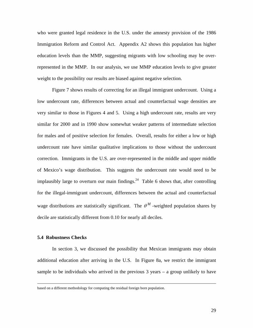
5.1 Actual and Counterfactual Wage Density Estimates

The results for Mexican males in 1990 are in Figures 4a and 4b. Although the

counterfactual density for Mexican immigrants is close to the actual density of Mexican

residents, some clear differences are apparent. Contrary to the negative-selection

hypothesis, it is not the lowest-wage males who exhibit a stronger tendency to migrate to

the U.S. For Mexican immigrants, there is less mass in the lower half of the wage density

and more mass in the upper half, when compared with the actual wage density of Mexico

residents. This is seen more clearly in Figure 4b, which shows the difference between the

counterfactual and actual wage densities. The immigrant-resident density difference is

negative from the left tail to just below zero, positive for middle and upper-middle wage

values, and negative for high wage values. This suggests that immigrant males are drawn

disproportionately from the middle and upper middle of Mexico’s wage distribution,

rather than from the bottom half. Low-wage and high-wage individuals appear least

likely to migrate to the U.S. These counterfactual wage densities support intermediate

selection of immigrant men in terms of observable skills.

The results for females in 1990, shown in Figures 4c and 4d, contain even less

support for negative selection. Except for high wage values, the counterfactual wage

density for immigrant females lies to the right of the actual wage density for resident

females. The immigrant-resident density difference is negative for low wage values,

strongly positive for upper-middle wage values, and zero for high wage values. For

women, there appears to be moderate positive selection of immigrants.

could in fact suffer from bias if the data do not conform to the Gaussian assumption. In order to avoid large bias in our estimates, we instead started with a bandwidth of 0.03 log wage units, and sequentially increased it until the resulting densities looked relatively smooth. This implied bandwidths in our final estimates of 0.07 log wage units.

24

Figures 5a-5d show counterfactual wage densities for immigrants in 2000,

evaluated at Mexican skill prices in 2000. For women, wage densities are very similar to

1990, again showing moderate positive selection of immigrants. For men, intermediate

selection of immigrants again appears, but less strongly. Comparing Figures 4b and 5b,

in 2000 immigrant men became somewhat less under-represented among low-wage

workers and somewhat more under-represented among high-wage workers

To compare changes in the pattern of immigrant selection more precisely, we

estimate the difference between immigrant (counterfactual) and resident (actual) wage

densities in 1990 and 2000, using 1990 skill prices. Figures 6a and 6b show the density

differences for 1990 and 2000 at 1990 skill prices (equations (17) and (20)) for males and

females and Figures 6c and 6d show the density double differences (equation (21)) for

males and females. For women, the density differences in the two years are very similar,

causing the double density difference to fluctuate around zero. For men, the density

difference in 2000 has less negative mass for low wage values and more negative mass

for high wage values, as suggested by Figures 4b and 5b. The double density difference

is thus positive below the mean, zero around the mean, and negative above the mean.

This is consistent with male immigrants becoming less under-represented at low wage

values and more under-represented at high wage values during the 1990’s.

Summarizing our results, Mexican immigrants in the U.S. are drawn dispropor-

tionately from the middle and upper-middle of Mexico’s wage distribution. Those most

likely to migrate abroad would earn medium-to-high wages in Mexico and those least

likely to migrate would earn low or very high wages in Mexico. In terms of observable

skills, males exhibit intermediate selection and females exhibit positive selection.

25

5.2 Parametric Results on Actual and Counterfactual Wage Distributions

An advantage of our nonparametric approach is that it characterizes differences in

resident and immigrant wage densities across the entire distribution. A disadvantage is

that it is difficult to assess whether the density differences are statistically significant. In

this section, we provide a parametric analog to the density differences reported in the last

section in order to gauge the statistical precision of these estimates. We see if the

counterfactual wage distribution for Mexican immigrants matches the actual wage

distribution for Mexican residents, when we summarize the distributions in terms of

quantiles. First, we sort wage observations for Mexican residents in a given year into

deciles. Then, we calculate the share of the population in each decile, weighting

observations by (which adjusts the Mexican resident population to reflect the

characteristics of the Mexican immigrant population in the U.S.). For each decile, we test

whether the -weighted shares are statistically different from 0.10. Negative selection

of immigrants in terms of observable skills would produce population shares above 0.10

for deciles below the median and below 0.10 for deciles above the median.

Mθ

Mθ

Table 6 reports the results. For males in 1990, immigrant population shares are

below 0.10 in the first four deciles, above 0.10 in the 5th to 9th deciles, and below 0.10 in

the 10th decile. All shares, except for the 4th decile, are statistically different from 0.10 at

a 5% level of significance. This pattern reinforces the results in Figure 4, which shows

that immigrants are over-represented in the upper middle of the wage distribution. For

males in 2000, results are similar, except that immigrants are no longer under-represented

in the 4th decile and are now under-represented in the 9th decile. This is consistent with

the results in Figure 6, which suggest that during 1990’s male Mexican immigrants

26

became somewhat less positively selected. For females in 1990, immigrant population

shares are below 0.10 in the first four deciles, close to 0.10 in the 5th decile, and greater

than 0.10 in the 6th to 10th deciles. All shares, expect for the 5th decile, are statistically

different from 0.10 at the 5% level. This is also consistent with Figure 4, in which female

immigrants from Mexico appear to be positively selected. For females in 2000, the

results are similar. Table 6 suggests the differences between actual and counterfactual

wage densities in Figures 4 and 5, though small, are statistically significant.

5.3 Correcting for the Undercount of Illegal Immigrants

As discussed in section 3, the U.S. census appears to undercount illegal

immigrants. If undercounted immigrants have low education levels, then our results

could be biased against finding negative selection. We cannot remedy this problem

directly, since we lack data on which immigrants are illegal within our sample. However,

we do have data from other sources on the characteristics of illegal immigrants.

We repeat the exercises from the previous section, but now modify the immigrant

sample so that the sampling weights for the logit analysis used to construct the

counterfactuals correspond to those of a synthetic sample in which there is no illegal-

immigrant undercount. We re-weight the original sample so that: i) the new weights

reflect an increase in the total Mexican immigrant population in the U.S., corresponding

to the estimated number of uncounted illegal immigrants, and ii) the re-weighting

procedure increases the population size to a greater extent for education groups in which

out-of-sample evidence suggests that illegal immigrants are concentrated.

Given multiple estimates of the illegal undercount, we report results based on

both Census Bureau and INS estimates of the illegal Mexican population. The Census

27

Bureau (Costanzo et al., 2001) estimates put the number of Mexican illegal immigrants

counted in the U.S. census at 1 million in 1990 and 3.9 million in 2000. Using Census

undercount rates of 20% in 1990 and 15% in 2000, the number of Mexican illegal

immigrants would be 1.3 million in 1990 – implying a 5.9% increase in the Mexican

immigrant population counted in the census – and 4.6 million in 2000 – implying a 7.4%

population increase. For the Census Bureau-based estimates, we re-weight the original

sample to increase the populations by these percentages. The INS (2003) puts the illegal

Mexican population at 2.0 million in 1990 and 4.8 million in 2000. These figures already

take into account undercount assumptions and imply a much higher undercount rate for

1990.23 For the INS-based estimates, we re-weight the original sample to increase the

populations by the implied percentages. We call the Census Bureau-based estimate the

low-undercount estimate and the INS-based estimate the high-undercount estimate.

To make this increased population have the characteristics of illegal immigrants,

we adjust the weights by schooling group. The “new” population is assumed to follow

the distribution of immigrants by schooling in Orrenius (1999), shown in Appendix A2.

This distribution is based on the Mexican Migration Project (MMP), a household survey

in rural Mexican communities over the period 1987-1997 where migration to the U.S.

tends to be high (Durand et al., 1996; Massey et al., 1994). A high fraction of migrants in

the MMP report having entered the U.S. illegally. Schooling levels of this group are

much lower than of Mexican immigrants in the U.S. census or of Mexican residents in

the Mexico census. A second data source on illegal immigrants is the Survey of Newly

Legalized Persons in California, from 1989, which covered undocumented immigrants

23 The INS estimate of 4.8 million illegal Mexican immigrants in 2000 is based on an assumed undercount rate 10%, which is less than the 15% undercount rate in Costanzo et al (2001) for that year. However, the INS estimates are

28

who were granted legal residence in the U.S. under the amnesty provision of the 1986

Immigration Reform and Control Act. Appendix A2 shows this population has higher

education levels than the MMP, suggesting migrants with low schooling may be over-

represented in the MMP. In our analysis, we use MMP education levels to give greater

weight to the possibility our results are biased against negative selection.

Figure 7 shows results of correcting for an illegal immigrant undercount. Using a

low undercount rate, differences between actual and counterfactual wage densities are

very similar to those in Figures 4 and 5. Using a high undercount rate, results are very

similar for 2000 and in 1990 show somewhat weaker patterns of intermediate selection

for males and of positive selection for females. Overall, results for either a low or high

undercount rate have similar qualitative implications to those without the undercount

correction. Immigrants in the U.S. are over-represented in the middle and upper middle

of Mexico’s wage distribution. This suggests the undercount rate would need to be

implausibly large to overturn our main findings.24 Table 6 shows that, after controlling

for the illegal-immigrant undercount, differences between the actual and counterfactual

wage distributions are statistically significant. The -weighted population shares by

decile are statistically different from 0.10 for nearly all deciles.

Mθ

5.4 Robustness Checks

In section 3, we discussed the possibility that Mexican immigrants may obtain

additional education after arriving in the U.S. In Figure 8a, we restrict the immigrant

sample to be individuals who arrived in the previous 3 years – a group unlikely to have

based on a different methodology for computing the residual foreign born population.

29

obtained U.S. schooling. The estimated density differences are very similar to those in

Figures 4 and 5. There again appears to be intermediate selection of immigrant men and

positive selection of immigrant women. An alternative way to address this issue would

be to adjust for the bunching of immigrants at 12 years of education. In unreported

results we combined individuals with 9 to 12 years of education into a single schooling

category. This addresses the concern that some immigrants with 12 years of schooling

may have obtained a GED, or, in response to cultural pressure, may overstate their

educational attainment. Again, these results are very similar to those reported.25

There remains the concern that education may be correlated with unobserved

characteristics that affect the migration decision, in which case our results might

exaggerate the extent of positive selection. Following the discussion in section 3, we

examine the importance of unobservables by restricting the sample of Mexican residents

to whom we compare Mexican immigrants. In Figure 8b, we construct immigrant-

resident density differences (evaluated at 1990 skill prices) using the sample of Mexican

residents who live in high-migration states (see note 18). Migration rates in these states

are 3.5 times those in the rest of the country, suggesting the presence of regional

migration networks. Relative to Figures 4 and 5, Figure 8b shows stronger evidence of

positive selection for both men and women. Given Table 3, which shows that residents

of high-migration states have low schooling levels relatives to either Mexican immigrants

in the U.S. or to residents in Mexico overall, this does not come as a surprise.

In Figure 8c, we limit the sample of Mexican residents to individuals who moved

24 Other results based on data in which illegal immigrants are over-represented tend to support our findings. Using the MMP, Orrenius and Zavodny (2004) find that migrants tend to come from the middle of the schooling distribution. 25 Results are also very similar when we expand the immigrant population to those at least 16 years old at U.S. entry.

30

between states in the previous five years. Similar to external migrants, internal migrants

may be highly driven or motivated, which may be important unobserved determinants of

the migration decision. Relative to Figures 4 and 5, there is somewhat weaker evidence

of intermediate selection for men. Immigrant men are still over-represented in the middle

of the wage distribution, but are now more under-represented in the upper tail. For

women, positive selection is modest in 1990, but appears quite strongly in 2000. Overall,

the qualitative patterns are broadly similar to previous results. Immigrants remain

concentrated in the middle or upper-middle of Mexico’s wage distribution.26

We have argued that it is important to hold constant how skill prices affect labor-

force participation when comparing wage distributions across workers in different

countries. So far, we have used skill prices and labor-force participation in Mexico as the

basis for these comparisons. For evaluating immigrant selection, it is no less valid to use

U.S. skill prices and labor-force participation. As a consistency check on our results, we

estimated the distribution of wages that would obtain if residents of Mexico were paid

according to U.S. skill prices and participated in the labor force as do Mexican

immigrants and then compared this to the actual wage distribution for Mexican

immigrants. In unreported results, we find that neither for males nor for females is there

support for negative selection of Mexican immigrants in terms of observable skills.

Resident males are under-represented in the middle and upper middle of the immigrant

wage distribution and over-represented in the upper tail, consistent with intermediate

selection of immigrants. Resident females are under-represented in the upper middle part

of the wage distribution, consistent with moderate positive selection of immigrants.

26 U.S. return migrants are another potential sample to whom to compare Mexican immigrants. However, sample sizes for this group (see Table 3) are very small, complicating estimation of wage densities.

31

6. Discussion

In this paper, we use data on residents of Mexico and Mexican immigrants in the

U.S. to test Borjas’ (1987) negative-selection hypothesis that the less skilled are those

most likely to migrate from countries with high returns to skill and high earnings

inequality to countries with low returns to skill and low earnings inequality. Our results

are inconsistent with the negative selection of Mexican immigrants in the U.S. For

Mexican-born males, there is evidence of intermediate selection and for Mexican-born

females there is evidence of positive selection. Those most likely to migrate are young

adults with moderately high schooling. Were these immigrants to return to Mexico, they

would to tend to fall in the middle or upper portions of Mexico’s wage distribution.

To arrive at these results, we construct counterfactual wage densities for Mexican

immigrants in the U.S., in which we use their observed characteristics to project the

wages they would earn in Mexico and under current patterns of wage determination in the

country. The results are robust to controlling for undercounts of illegal immigrants in the

U.S. census, for opportunities to gain education in the U.S., for changes in skill prices

over time, and for access to regional migration networks.

There are several important caveats to our results. We cannot say how the return

of Mexican immigrants in the U.S. would affect Mexico’s wage structure. Other work

gives some guidance on this issue. Using data for 1970-2000, Mishra (2003) estimates an

elasticity of wages with respect to emigration in Mexico of 0.4. Given the concentration

of emigrants among moderately well-educated young adults, wage gains in Mexico have

been largest among 25 to 40 year olds with 12 to 15 years of schooling. Wage changes

are not the only consequence of emigration. In 2003, remittances by immigrants in the

32

U.S. were 2% of Mexico’s GDP. In high-migration regions, remittances appear to have

raised investments in small businesses (Woodruff and Zenteno, 2001).

Another caveat is that our findings against negative selection and in favor of

intermediate or positive selection are in terms of observable characteristics only. We

cannot say whether the unobserved skills of Mexican immigrants in the U.S. are high or

low relative to those who remain in Mexico. There is some evidence on the role of

unobservables in the migration decision. When we limit the comparison to external and

internal migrants, individuals who may posses similar unobserved characteristics, we

continue to find evidence against the negative selection of Mexican immigrants.

That immigrants from Mexico appear to be relatively high-wage individuals is

surprising. The estimated returns to education are higher in Mexico than in the U.S.,

suggesting that low-wage individuals from Mexico would have most to gain from

migrating to the U.S. Heterogeneity in migration costs is one way to reconcile these

facts. The more educated may be better able to negotiate the migration process, they may

have better access to migration networks in the U.S., or they may be less subject to credit

constraints in financing migration. Also, higher discount rates or greater risk aversion

among the low-skilled may make migration abroad relatively less attractive for this

group. Finally, a “Washington apples” effect (Alchian and Allen, 1964) may also

contribute to positive selection of migrants. Given long queues for U.S. legal admission,

two-thirds of Mexicans immigrate illegally on their first attempt. Enforcement against

illegal immigration may act as a head tax, penalizing the less skilled. If more-skilled and

less-skilled illegal immigrants compete for jobs in the U.S., it will be efficient, given

fixed migration costs, to fill jobs with more skilled individuals first.

33

Appendix

A.1 Logit Estimation of the Probability of Migration to the U.S.

Males 1990 Males 2000 Variable Coeff. St. Error Coeff. St. Error

Years 1 to 4 -1.713 0.37 -1.206 0.392 of 5 to 8 -3.232 0.329 -1.233 0.302

Schooling 9 -3.844 0.501 -3.443 0.409 10 to 11 -3.756 0.604 -1.663 0.44 12 -3.208 0.443 -0.907 0.339 13 to 15 -5.88 0.596 -4.363 0.471 16+ -3.537 0.679 -1.582 0.471

Age 0.164 0.019 0.207 0.017 Age^2 -0.28 0.026 -0.328 0.022

Married 3.584 0.265 4.734 0.204 Age* 1 to 4 0.042 0.02 -0.022 0.021

5 to 8 0.158 0.018 0.037 0.016 9 0.17 0.03 0.122 0.024 10 to 11 0.198 0.037 0.058 0.025 12 0.22 0.026 0.059 0.019 13 to 15 0.331 0.037 0.224 0.028 16+ 0.118 0.038 0 0.026

Age^2* 1 to 4 -0.025 0.025 0.044 0.026 5 to 8 -0.167 0.024 -0.031 0.021 9 -0.179 0.043 -0.145 0.033 10 to 11 -0.197 0.053 -0.016 0.035 12 -0.256 0.037 -0.055 0.025 13 to 15 -0.39 0.054 -0.262 0.038 16+ -0.11 0.05 0.023 0.034

Married* 1 to 4 -0.147 0.068 -0.255 0.072 5 to 8 -0.403 0.057 -0.415 0.054 9 -0.492 0.076 -0.573 0.063 10 to 11 -0.877 0.087 -0.869 0.074 12 -0.62 0.067 -0.568 0.059 13 to 15 -0.356 0.085 -0.311 0.078 16+ -0.193 0.107 -0.324 0.08

Pseudo R2 0.046 0.065 Notes: This table shows logit estimation results in which the dependent variable is 1 if an individual lives in the U.S. and 0 if an individual lives in Mexico. The sample is Mexico-born men 21-65 years of age in the U.S. and Mexico population censuses in 1990 or

34

2000. Regressors are age, age squared, dummy variables for schooling and marital status, and interactions among these variables. Unreported results for women are similar. For females, we also include as regressors the number of children born to the individual and its interactions with age and schooling. A.2 Educational Attainment for Mexican Illegal Immigrants

Mexico Migration Project Survey of Newly Legalized Persons

Years of Education Migrants Non-migrants Years of Education Immigrants 0 to 1 27.1 23.3 0 5.6 2 to 4 32.6 22.1 1 to 3 14.6 5 to 6 23.1 22.5 4 to 6 41.6 7 to 9 8.9 11.7 7 to 9 22.2

10 to 12 4.3 8.1 10 to 12 12.8 13+ 4.1 12.3 13+ 3.2

% of trips to U.S. involving illegal entry 60.8 --

Notes: Columns 1-3 are from Orrenius (1999). The sample is 5,478 head of household males between 15 and 65 years of age, surveyed between 1987-1995 in 35 communities in western Mexico. Columns 4 and 5 are based on California Health and Welfare Agency (1989). The sample is 4,091 Mexico-born individuals (men and women) residing in California in 1989 who arrived in the U.S. as illegal immigrants and who were granted permanent legal residence under the amnesty provision of the 1986 Immigration Reform and Control Act. Reported education levels are a weighted average of those granted amnesty based on having arrived in the U.S. prior to 1982 (60% of those legalized) and those granted amnesty as special agricultural workers (40% of those legalized). The education categories shown above are as reported in the original data sources, which do not exactly match the categories we report in Table 2. Since the Mexican census reports the exact number of years of schooling completed, we are able to use the above figures to re-weight the samples, as described in section 5.3.

35

References Alchian, Armen, and William Allen. 1964. University Economics. Belmont, CA.

Wadsworth. Ariola, Jim and Chinhui Juhn. 2003. “Wage Inequality in Post-Reform Mexico.”

Mimeo, University of Houston. Baker, Michael, and Dwayne Benjamin. 1997. “The Role of the Family in Immigrants’

Labor-Market Activity: An Evaluation of Alternative Explanations.” American Economic Review 87: 705-729.

Bean, Frank, Rodolf Corona, Rodolf Tuiran, Karen A. Woodrow-Lafield, and Jennifer Van Hook. 2001. “Circular, Invisible, and Ambiguous Migrants,” Demography, 38(3), August, 411-422.

Bean, Frank, Jennifer Hook, Karen Woodrow-Lafield. 2001. “Estimates of the Number of Unauthorized Migrants Residing in the United States.” Pew Hispanic Center.

Beine, Michel, Frederic Docquier, and Hillel Rapoport. 2001. “Brain Drain and Economic Growth.” Journal of Development Economics 64(1): 275-289.

Betts, Julian and Magnus Lofstrom. 1998. “The Educational Attainment of Immigrants: Trends and Implications.” NBER Working Paper No. 6757.

Borjas, George J. 1987. “Self-Selection and the Earnings of Immigrants.” American Economic Review 77(4): 531-553.

Borjas, George, J. 1991. “Immigration and Self-Selection.” In John Abowd and Richard Freeman, eds., Immigration, Trade, and the Labor Market. Chicago: University of Chicago Press, pp. 29-76.

Borjas, George J. 1995. “Assimilation and Changes in Cohort Quality Revisited: What Happened to Immigrant Earnings in the 1980s?” Journal of Labor Economics 13(2): 201-245.

Borjas, George J. 1996. “The Earnings of Mexican Immigrants in the United States.” Journal of Development Economics 51: 69-98.

Borjas, George J. 1999. “The Economic Analysis of Immigration.” In Orley C. Ashenfelter and David Card, eds., Handbook of Labor Economics, Amsterdam: North-Holland, pp. 1697-1760.

Borjas, George J. 2003. “The Labor Demand Curve is Downward Sloping: Reexamining the Impact of Immigration on the Labor Market.” Quarterly Journal of Economics 108(4): 1335-1374.

Borjas, George J., and Bernt Bratsberg. 1996. “Who Leaves? The Outmigration of the Foreign Born.” Review of Economics and Statistics, 78(1): 165-76.

Borjas, George J., Stephen G. Bronars, and Stephen J. Trejo. 1992. “Self-Selection and Internal Migration in the United States.” Journal of Urban Economics 32(2): 159-185.

Borjas, George J., Richard B. Freeman, and Lawrence F. Katz. 1997. "How Much Do Immigration and Trade Affect Labor Market Outcomes?" Brookings Papers on Economic Activity 1: 1-90.

Bound, John, and Harry Holzer. 2000. “Demand Shifts, Population Adjustments and Labor Market Outcomes during the 1980s.” Journal of Labor Economics 18(1): 20-54.

36

Bratsberg, Bernt and James F. Ragan, Jr. 2002. “The Impact of Host-Country Schooling on Earnings – A Study of Males Immigrants in the United States.” Forthcoming, Journal of Human Resources.

Butcher, Kristin F. and John DiNardo. 2002. “The Immigrant and Native-Born Wage Distributions: Evidence from United States Censuses.” Industrial and Labor Relations Review, forthcoming.

California Health and Welfare Agency. 1989. A Survey of Newly Legalized Persons in California. San Diego, CA: Comprehensive Adult Student Assessment System.

Cameron, Stephen V., and James J. Heckman. 1993. “The Nonequivalence of High School Equivalents,” Journal of Labor Economics, Vol. 11, No. 1, Part 1: Essays in Honor of Jacob Mincer. (Jan., 1993), pp. 1-47.

Carrington, William J. and Detragiache, Enrica. 1998. “How Big is the Brain Drain?” IMF Working Paper WP/98/102.

Chiquiar, Daniel. 2003. Essays on the Regional Implications of Globalization: The Case of Mexico. Ph.D. Dissertation, University of California, San Diego.

Chiswick, Barry. 1978. “The Effect of Americanization on the Earnings of Foreign-born Men.” Journal of Political Economy 86(5): 897-921.

Clark, Melissa A. and David A. Jaeger. 2002. “Natives, the Foreign Born, and High School Equivalents: New Evidence on Returns to the GED.” Working Paper #462, Princeton University Industrial Relations Section.

Cornelius, Wayne A. and Enrico A. Marselli. 2001. “The Changing Profile of Mexican Migrants to the United States: New Evidence from California and Mexico.” Latin American Research Review, forthcoming.

Costanzo, Joe, Cynthia Davis, Caribert Irazi, Daniel Goodkind and Roberto Ramirez. 2001. “Evaluating Components of International Migration: The Residual Foreign Born Population.” U.S. Bureau of the Census, Division Working Paper No. 61.

Cragg, Michael I., and Mario Epelbaum. 1996. “Why Has Wage Dispersion Grown in Mexico?” Journal of Development Economics, 51(1), October, pp. 99-116.

DiNardo, John, M. Fortin, and Thomas Lemieux. 1996. “Labor Market Institutions and the Distribution of Wages, 1973-1992: A Semiparametric Approach.” Econometrica 64(5): 1001-1044.

Durand, Jorge, William Kandel, Emilio Parrado and Douglas S. Massey. 1996. “International Migration and Development in Mexican Communities.” Demography 33(2): 249-264.

Durand, Jorge, Douglas S. Massey, and Rene M. Zenteno. 2001. “Mexican Immigration in the United States.” Latin American Research Review 36(1): 107-127.

Feliciano, Zadia. 2001. “The Skill and Economic Performance of Mexican Immigrants from 1910 to 1990.” Explorations in Economic History 38: 386-409.

Grogger, Jeffrey, and Stephen J. Trejo. 2002. Moving behind or Moving up? The Intergenerational Progress of Mexican Americans. San Francisco, CA: Public Policy Institute of California.

Hanson, Gordon H., and Antonio Spilimbergo. 1999. "Illegal Immigration, Border Enforcement and Relative Wages: Evidence from Apprehensions at the U.S.-Mexico Border," American Economic Review, 89: 1337-57.

Heckman, James, and Bo Honore. 1990. “The Empirical Content of the Roy Model.” Econometrica, 58(5): 1121-49.

37

Immigration and Naturalization Service. 2003. “Estimates of the Unauthorized Immigrant Population Residing in the United States: 1990 to 2000.”

LaLonde, Robert and Robert Topel. 1992. "The Assimilation of Immigrants in the U.S. Labor Market." In George J. Borjas and Richard Freeman, eds, Immigration and the Work Force: Economic Consequences for the United States and Source Areas, (Chicago, IL: University of Chicago Press): 67-92.

LaLonde, Robert and Robert Topel. 1997. “Economic Impact of International Migration and Migrants.” In Mark R. Rosenzweig and Oded Stark, eds., Handbook of Population and Family Economics, (Amsterdam: Elsevier Science): 799-850.

Massey, Douglas S., L. Goldring, and Jorge Durand. 1994. “Continuities in Transnational Migration: An Analysis of Nineteen Mexican Communities.” American Journal of Sociology 99(6): 1492-1533.

Mishra, Prachi. 2003. “Emigration and Wages in Source Countries: Evidence from Mexico.” Mimeo, Columbia University.

Munshi, Kaivan. 2003. “Networks in the Modern Economy: Mexican Migrants in the US Labor Market.” Quarterly Journal of Economics, 118(2):549-597. .

Murnane, Richard J., John B. Willett, and John H. Tyler. 2000. “Who Benefits from Obtaining a GED? Evidence from High School and Beyond.” Review of Economics and Statistics, 82(1), February, 285-326.

Orrenius, Pia M. 1999. “Family Networks, Coyote Prices, and the Rural Economy in Migration from Western Mexico: 1965-1994.” Mimeo, Dallas Federal Reserve.

Orrenius, Pia M. and Madeline Zavodny. 2004. “Self-Selection among Undocumented Immigrants from Mexico.” Journal of Development Economics, forthcoming.

Passel, Jeffrey, Randy Capps, and Michael Fix. 2004. “Undocumented Immigration: Facts and Figures.” Urban Institute.

Ramos, Fernando. 1992. “Out-Migration and Return Migration of Puerto Ricans.” George Borjas and Richard Freeman, eds., Immigration and the Work Force. Chicago: NBER and University of Chicago Press, pp. 49-66.

Roy, A.D. 1951. “Some Thoughts on the Distribution of Earnings.” Oxford Economic Papers 3: 135-146.

Silverman, B. 1986. Density Estimation for Statistics and Data Analysis. London: Chapman and Hall.

Sjaastad, Larry. A. 1962. "The Costs and Returns of Human Migration." Journal of Political Economy, 70(1), pp. 80-93

Smith, James and Barry Edmonston. 1997. The New Americans: Economic, Demographic and Fiscal Effects of Immigration. National Academy Press: Washington, D.C.

Trejo, Stephen J. 1997. “Why do Mexican Americans Earn Low Wages?” Journal of Political Economy 105(6): 1235-1268.

Woodruff, Christopher and Rene M. Zenteno. 2001. “Remittances and Microenterprises in Mexico.” Mimeo, UC San Diego.

38

Table 1: Share of U.S. Immigrants from Mexico in Population of Mexico, 1990 and 2000

(percent)

Males Females Age Cohort % Residing in U.S. % Residing in U.S.

Age in 1990 Age in 2000 1990 2000 Change 1990 2000 Change

-- 16 to 25 -- 11.99 -- -- 7.68 --

16 to 25 26 to 35 7.57 17.53 9.96 4.89 12.62 7.73

26 to 35 36 to 45 10.87 15.49 4.62 7.69 11.90 4.21

36 to45 46 to 55 9.18 12.21 3.03 7.47 10.44 2.97

46 to 55 56 to 65 7.00 8.64 1.64 6.44 8.36 1.92

56 to 65 -- 5.70 -- -- 5.84 -- --

Notes: For 1990 and 2000, this table shows Mexican immigrants in the U.S. as a percentage of the population of individuals born in Mexico (equal to the sum of the Mexico-born residing in Mexico and the Mexico-born residing in the U.S.) by age and sex categories.

39

Table 2a: Summary Statistics for Males, 1990

U.S. Residents Mexico Mex. Immigrants Other U.S.

Variable Residents Recent All Immigrants Natives Age 36.8 33.2 39.1 42.7 40.0

Highest Grade 0 0.138 0.133 0.146 0.040 0.005 of Schooling 1 to 4 0.223 0.125 0.167 0.029 0.005 Completed 5 to 8 0.276 0.289 0.302 0.095 0.039

(%) 9 0.115 0.081 0.068 0.028 0.024 0 to 9 0.752 0.628 0.683 0.192 0.073

10 to 11 0.048 0.059 0.050 0.041 0.069 12 0.066 0.178 0.152 0.234 0.333 13 to 15 0.049 0.087 0.077 0.200 0.284 10 to 15 0.163 0.324 0.279 0.475 0.686 16+ 0.084 0.048 0.038 0.334 0.242 Wage Earners (%) 0.726 0.832 0.830 0.792 0.833

Hourly wage 1.39 7.17 8.23 14.57 14.27 N 163798 22207 39780 152047 609786

Table 2b: Summary Statistics for Females, 1990

U.S. Residents Mexico Mex. Immigrants Other U.S. Residents Recent All Immigrants Natives

Age 36.7 34.3 40.4 43.8 40.2 Highest Grade 0 0.188 0.138 0.146 0.048 0.004 of Schooling 1 to 4 0.228 0.142 0.169 0.036 0.003 Completed 5 to 8 0.274 0.298 0.318 0.107 0.031

(%) 9 0.100 0.074 0.064 0.031 0.023 0 to 9 0.790 0.652 0.697 0.222 0.061

10 to 11 0.044 0.047 0.044 0.045 0.073 12 0.077 0.174 0.156 0.298 0.370 13 to 15 0.045 0.084 0.073 0.207 0.299 10 to 15 0.166 0.305 0.273 0.550 0.742 16+ 0.044 0.042 0.031 0.229 0.197 Wage Earners (%) 0.207 0.440 0.465 0.597 0.709

Hourly wage 1.34 6.08 6.57 10.19 9.98 N 178726 18640 34381 168222 650229

40

Table 2c: Summary Statistics for Males, 2000

U.S. Residents Mexico Mex. Immigrants Other U.S.

Variable Residents Recent All Immigrants Natives Age 37.2 33.2 39.5 43.5 41.4

Highest Grade 0 0.069 0.096 0.127 0.035 0.005 of Schooling 1 to 4 0.166 0.057 0.080 0.013 0.002 Completed 5 to 8 0.270 0.300 0.307 0.071 0.021

(%) 9 0.189 0.105 0.087 0.025 0.017 0 to 9 0.694 0.558 0.601 0.144 0.045

10 to 11 0.045 0.064 0.055 0.036 0.053 12 0.101 0.245 0.212 0.240 0.328 13 to 15 0.047 0.079 0.083 0.186 0.308 10 to 15 0.193 0.388 0.350 0.462 0.689 16+ 0.113 0.054 0.050 0.394 0.267 Wage Earners (%) 0.740 0.789 0.800 0.800 0.824

Hourly wage 1.21 7.90 8.72 15.23 14.88 N 215804 39073 80453 222605 652895

Table 2d: Summary Statistics for Females, 2000

U.S. Residents Mexico Mex. Immigrants Other U.S. Residents Recent All Immigrants Natives

Age 37.0 34.8 40.5 44.0 41.5 Highest Grade 0 0.092 0.113 0.133 0.042 0.004 of Schooling 1 to 4 0.179 0.066 0.087 0.017 0.001 Completed 5 to 8 0.28 0.301 0.315 0.079 0.016

(%) 9 0.174 0.101 0.085 0.025 0.015 0 to 9 0.725 0.581 0.620 0.163 0.036

10 to 11 0.04 0.054 0.049 0.037 0.050 12 0.112 0.228 0.204 0.272 0.323 13 to 15 0.042 0.079 0.079 0.209 0.337 10 to 15 0.194 0.361 0.332 0.518 0.710 16+ 0.080 0.058 0.048 0.320 0.255 Wage Earners (%) 0.321 0.418 0.463 0.605 0.739

Hourly wage 1.24 6.90 7.30 11.57 11.28 N 235086 35277 72967 247970 693483

41

Table 3: Educational Attainment for Subsamples of the Mexico Born Mexico Residents Mexican Immigrants in US, 26-35 Yrs Old High Emig. States Internal Migrants Return Emigrants 26-35 Year Olds 0-3 Yrs 4+ Yrs 0-3 Yrs 4+ Yrs

Males 1990 2000 1990 2000 1990 2000 1990 2000 1990 1990 2000 2000 0 0.190 0.093 0.087 0.042 0.094 0.039 0.086 0.036 0.113 0.113 0.076 0.078 1-4 0.264 0.203 0.141 0.106 0.211 0.135 0.172 0.103 0.103 0.112 0.045 0.043

Highest 5-8 0.263 0.286 0.262 0.238 0.368 0.372 0.297 0.263 0.278 0.309 0.303 0.275Grade of 9 0.096 0.169 0.130 0.203 0.139 0.222 0.129 0.246 0.082 0.081 0.114 0.116

Schooling 0-9 0.813 0.751 0.620 0.589 0.812 0.768 0.684 0.648 0.576 0.615 0.538 0.512(%) 10-11 0.034 0.034 0.061 0.052 0.039 0.041 0.058 0.059 0.061 0.057 0.064 0.067

12 0.055 0.081 0.090 0.124 0.057 0.093 0.082 0.129 0.188 0.189 0.260 0.278 13-15 0.037 0.037 0.075 0.063 0.022 0.035 0.057 0.044 0.103 0.096 0.075 0.098 10-15 0.126 0.152 0.226 0.239 0.118 0.169 0.197 0.232 0.352 0.342 0.399 0.443 16+ 0.063 0.096 0.154 0.171 0.070 0.062 0.118 0.121 0.073 0.043 0.062 0.046

N 54,778 78,330 8,913 9,694 459 1,695 52,864 68,206 3,599 9,121 9,358 15,839Females

0 0.233 0.113 0.123 0.051 0.093 0.019 0.121 0.047 0.097 0.109 0.070 0.078 1-4 0.265 0.213 0.159 0.117 0.173 0.109 0.196 0.116 0.113 0.121 0.041 0.043

Highest 5-8 0.259 0.297 0.278 0.270 0.360 0.336 0.309 0.278 0.278 0.348 0.269 0.294Grade of 9 0.084 0.157 0.122 0.198 0.121 0.225 0.109 0.219 0.076 0.082 0.112 0.125

Schooling 0-9 0.841 0.780 0.682 0.636 0.747 0.689 0.735 0.660 0.564 0.660 0.492 0.540(%) 10-11 0.031 0.030 0.063 0.055 0.033 0.053 0.053 0.054 0.052 0.045 0.056 0.062

12 0.061 0.090 0.106 0.141 0.117 0.163 0.090 0.145 0.205 0.170 0.276 0.253 13-15 0.035 0.036 0.073 0.055 0.065 0.046 0.056 0.039 0.106 0.088 0.083 0.090 10-15 0.127 0.156 0.242 0.251 0.215 0.262 0.199 0.238 0.363 0.303 0.415 0.405 16+ 0.032 0.064 0.075 0.112 0.037 0.049 0.065 0.103 0.074 0.038 0.093 0.055

N 61,297 88,818 9,491 10,141 214 733 58,069 75,625 3,211 7,057 6,575 16,173

Table 4: Labor-Force Participation Rates Residents of Mexico Recent Mex. Immigrants

Years of Age Category Age Category Schooling 26-35 36-45 46-55 56-65 26-35 36-45 46-55 56-65

(a) Males, 1990 0 0.63 0.65 0.61 0.50 0.81 0.83 0.81 0.67

1 to 4 0.72 0.72 0.66 0.54 0.86 0.85 0.82 0.70 5 to 8 0.79 0.81 0.75 0.58 0.86 0.85 0.82 0.65

9 0.84 0.85 0.78 0.59 0.85 0.86 0.79 0.66 10 to 11 0.87 0.88 0.77 0.60 0.85 0.85 0.74 0.72

12 0.85 0.88 0.81 0.59 0.86 0.84 0.81 0.66 13 to 15 0.85 0.89 0.83 0.60 0.87 0.87 0.76 0.70

16+ 0.86 0.91 0.85 0.67 0.87 0.83 0.89 0.72 (b) Males, 2000 0 0.60 0.61 0.57 0.45 0.73 0.77 0.74 0.59

1 to 4 0.70 0.69 0.64 0.49 0.77 0.82 0.72 0.55 5 to 8 0.78 0.78 0.75 0.54 0.82 0.79 0.76 0.66

9 0.84 0.84 0.79 0.56 0.81 0.81 0.82 0.75 10 to 11 0.87 0.88 0.81 0.60 0.80 0.79 0.80 0.63

12 0.86 0.87 0.78 0.51 0.83 0.82 0.79 0.58 13 to 15 0.82 0.91 0.82 0.54 0.85 0.88 0.86 0.55

16+ 0.86 0.90 0.87 0.66 0.86 0.87 0.78 0.69 (c) Females, 1990 0 0.09 0.09 0.08 0.07 0.41 0.43 0.36 0.13

1 to 4 0.10 0.11 0.09 0.07 0.44 0.52 0.42 0.20 5 to 8 0.16 0.19 0.16 0.10 0.46 0.50 0.44 0.23

9 0.28 0.29 0.27 0.10 0.46 0.52 0.53 0.28 10 to 11 0.36 0.40 0.33 0.14 0.46 0.46 0.47 0.43

12 0.47 0.48 0.40 0.20 0.47 0.57 0.45 0.24 13 to 15 0.57 0.56 0.48 0.27 0.52 0.53 0.58 0.30

16+ 0.57 0.63 0.53 0.31 0.53 0.62 0.50 0.34 (c) Females, 2000 0 0.16 0.19 0.16 0.13 0.36 0.44 0.34 0.19

1 to 4 0.21 0.22 0.20 0.12 0.41 0.44 0.40 0.18 5 to 8 0.25 0.29 0.27 0.17 0.38 0.46 0.41 0.19

9 0.33 0.39 0.36 0.19 0.41 0.51 0.45 0.23 10 to 11 0.41 0.48 0.43 0.22 0.40 0.51 0.35 0.25

12 0.47 0.51 0.45 0.27 0.43 0.50 0.48 0.24 13 to 15 0.57 0.67 0.52 0.23 0.53 0.55 0.56 0.34

16+ 0.67 0.71 0.63 0.35 0.50 0.46 0.54 0.22

44

Table 5: OLS Wage Regressions for Men, 1990 and 2000 Mexico Mexican Immigrants Other Mexican Mexican Immigrants Other Resident Recent All Immigrant Resident Recent All ImmigrantVariable 1990 1990 1990 1990 2000 2000 2000 2000

High 5 to 8 0.202 0.038 0.070 0.022 0.196 0.006 0.039 0.017 Grade (0.006) (0.011) (0.008) (0.010) (0.007) (0.011) (0.007) (0.010)

of 9 to 11 0.359 0.071 0.130 0.080 0.358 0.033 0.079 0.100 Schooling (0.008) (0.014) (0.011) (0.010) (0.007) (0.012) (0.008) (0.010) 12 0.551 0.115 0.163 0.202 0.605 0.112 0.154 0.202 (0.010) (0.013) (0.010) (0.008) (0.009) (0.011) (0.007) (0.009) 13 to 15 0.741 0.182 0.257 0.339 0.960 0.209 0.283 0.358 (0.012) (0.016) (0.012) (0.009) (0.013) (0.014) (0.009) (0.009) 16+ 1.096 0.416 0.487 0.690 1.328 0.460 0.493 0.783 (0.009) (0.020) (0.016) (0.008) (0.009) (0.016) (0.011) (0.008)

Age 26 to 35 0.110 0.060 0.059 0.116 0.126 0.068 0.069 0.154 (0.007) (0.012) (0.012) (0.010) (0.006) (0.010) (0.010) (0.011)

36 to 45 0.210 0.081 0.094 0.208 0.207 0.106 0.107 0.166 (0.008) (0.015) (0.014) (0.011) (0.007) (0.012) (0.011) (0.011) 46 to 55 0.240 0.075 0.055 0.194 0.242 0.079 0.086 0.118

(0.009) (0.019) (0.015) (0.011) (0.008) (0.015) (0.012) (0.011) 56 to 65 0.168 0.092 -0.007 0.095 0.195 0.076 0.023 0.046 (0.011) (0.029) (0.019) (0.012) (0.011) (0.023) (0.014) (0.012)

R Sqd. 0.233 0.063 0.140 0.248 0.354 0.062 0.098 0.212N 112,111 17,939 32,011 112,552 142,113 30,036 62,551 164,864

Notes: See notes to Table 5, below.

45

Table 6: Counterfactual Wage Deciles

Decile Males 1990 Males 2000 Females 1990 Females 2000 (a) Main Sample 1 0.090 0.096 0.080 0.085 [0.089, 0.092] [0.094, 0.097] [0.077, 0.083] [0.083, 0.088]

2 0.092 0.097 0.083 0.087 [0.091, 0.094] [0.096, 0.099] [0.080, 0.086] [0.085, 0.089]

3 0.095 0.100 0.088 0.090 [0.094, 0.097] [0.099, 0.102] [0.085, 0.091] [0.087, 0.092]

4 0.099 0.102 0.093 0.093 [0.097, 0.100] [0.100, 0.103] [0.090, 0.097] [0.091, 0.095]

5 0.102 0.104 0.099 0.099 [0.101, 0.104] [0.103, 0.106] [0.096, 0.102] [0.097, 0.102]

6 0.105 0.104 0.109 0.105 [0.103, 0.106] [0.103, 0.106] [0.106, 0.112] [0.103, 0.108]

7 0.107 0.110 0.111 0.115 [0.105, 0.108] [0.108, 0.112] [0.108, 0.114] [0.113, 0.118]

8 0.110 0.108 0.115 0.111 [0.108, 0.112] [0.106, 0.109] [0.112, 0.119] [0.109, 0.114]

9 0.106 0.099 0.117 0.110 [0.104, 0.108] [0.097, 0.100] [0.114, 0.120] [0.107, 0.112]

10 0.093 0.081 0.104 0.104 [0.092, 0.095] [0.079, 0.082] [0.101, 0.108] [0.101, 0.106]

(b) Correcting for Illegal Immigrant Undercount 1 0.096 0.093 0.089 0.082 [0.094, 0.098] [0.091, 0.094] [0.086, 0.092] [0.080, 0.084]

2 0.097 0.095 0.089 0.085 [0.095, 0.098] [0.094, 0.097] [0.086, 0.092] [0.083, 0.087]

3 0.098 0.099 0.093 0.089 [0.096, 0.100] [0.098, 0.101] [0.090, 0.096] [0.086, 0.091]

4 0.100 0.101 0.096 0.092 [0.098, 0.102] [0.100, 0.103] [0.093, 0.100] [0.090, 0.094]

5 0.102 0.104 0.099 0.099 [0.101, 0.104] [0.102, 0.105] [0.096, 0.102] [0.097, 0.101]

6 0.104 0.105 0.106 0.107 [0.102, 0.106] [0.103, 0.106] [0.103, 0.109] [0.105, 0.109]

7 0.105 0.111 0.106 0.116 [0.103, 0.107] [0.110, 0.113] [0.103, 0.110] [0.114, 0.119]

8 0.106 0.109 0.109 0.113 [0.105, 0.108] [0.108, 0.111] [0.106, 0.113] [0.111, 0.115]

9 0.102 0.101 0.110 0.112 [0.100, 0.104] [0.099, 0.102] [0.107, 0.114] [0.110, 0.115]

10 0.090 0.083 0.101 0.105 [0.088, 0.092] [0.081, 0.084] [0.098, 0.104] [0.103, 0.108]

Notes: 95% confidence intervals are in brackets. See notes to Table 6 for other details.

46

Notes to Tables 2a-2d, 3: The sample is individuals 21-65 years old (in the U.S., excluding group quarters; in Mexico, excluding those not born in the country). Residents of Mexico in 1990 are the 1% microsample of the XII Censo General de Poblacion y Vivienda, 1990, and in 2000 are a 10% random sample of the 10% microsample of the XIII Censo General de Poblacion y Vivienda, 2000. Mexican and other immigrants are from the 1990 and 2000 5% U.S. PUMS; U.S. natives are from the 1990 and 2000 1% U.S. PUMS. Immigrants in the U.S. are restricted to be individuals 21 years or older at time of entry into the country. Recent immigrants are individuals who entered the U.S. during the period 1981-1990 for 1990 and 1991-2000 for 2000. Schooling variables show the percentage of individuals whose high grade completed is that indicated and wage earners shows the percentage of individuals with positive labor earnings. Wage levels are in 1990 U.S. dollars (see note 11 on how wages are constructed). Average wages in Mexico are for those individuals with average hourly earnings between $0.05 and $20 and in the U.S. are for those individuals with average hourly earnings between $1 and $100. See note 18 for the list of high-emigration states. Internal (return) migrants are individuals who lived in a different state (in the U.S.) five years previously. Notes to Table 4: The table shows the percentage of the population that reported positive labor earnings by year, age, and high year of schooling completed for residents of Mexico and for recent Mexican immigrants in the U.S. (individuals who arrived in U.S. during the previous ten years). Immigrants are those 21 years or older at time of U.S. entry. Notes to Table 5: The table reports OLS results for the log average hourly wage (see note 11 for details on wages). Heteroskedasticity-consistent standard errors are in parentheses. Samples are men 21-65 years of age, whose usual or average weekly hours of work are 10-80, and who are residents of Mexico (columns 1 and 5), Mexican immigrants in the U.S. who arrived during the previous ten years (columns 2 and 6), all Mexican immigrants in the U.S. (columns 3 and 7), or non-Mexico-born U.S. immigrants (columns 4 and 8). Immigrant samples exclude individuals aged 20 years or less at time of U.S. entry. The Mexican-resident sample includes individuals with hourly wages between $0.05 and $20 and U.S.-resident samples include individuals with hourly wages between $1 and $100 (in 1990 U.S. dollars). Regressors not shown are dummy variables for marital status, metro residence, and region (all columns); dummy variables for race (column 4 and 8); and dummy variables for year of U.S. entry (columns 2-4, 6-8). Notes to Table 6: This table reports the weighted share of the Mexico resident population that occupies a given decile of the wage distribution (95% confidence intervals are in brackets). Unweighted shares are by definition 0.10. The weights used to calculate the reported shares are those defined in equation (16), which adjust the characteristics of the Mexican resident population to reflect the characteristics of the Mexican immigrant population in the U.S. Mexican residents are individuals 21-65 years of age with positive labor earnings. Mexican immigrants are individuals 21-65 years of age who arrived in the U.S. in the previous 10 years. The weights are calculated using the logit results shown in Appendix A1. Part (a) shows results corresponding to Figures 4 and 5 (with no adjustment for the illegal-immigrant undercount) and part (b) shows results that correspond to Figure 7b (the sample adjusted for the high illegal-immigrant undercount).

47

Figure 1

lnw

s00 δ+µ

πµ−δ+µ es11

πµ

−µ e1

µ0

s* s

Figure 2

lnw

ssL

µ0

s11 es ππ δ−µ−δ+µ

s00 δ+µ

πµ−µ e1

sU

48

Figure 3:

Wage Densities for Residents of Mexico and Mexican Immigrants in the U.S.

(a) Males, 1990 (b) Males, 2000

lnw

Actual density: Mex Residents Actual density: Mex Imm in US

-3 -2 -1 0 1 2 3 4 5

0

.1

.2

.3

.4

.5

.6

.7

.8

.9

1

lnw

Actual density: Mex Residents Actual density: Mex Imm in US

-3 -2 -1 0 1 2 3 4 5

0

.1

.2

.3

.4

.5

.6

.7

.8

.9

1

lnw

Actual density: Mex Residents Actual density: Mex Imm in US

-3 -2 -1 0 1 2 3 4 5

0

.1

.2

.3

.4

.5

.6

.7

.8

.9

1

lnw

Actual density: Mex Residents Actual density: Mex Imm in US

-3 -2 -1 0 1 2 3 4 5

0

.1

.2

.3

.4

.5

.6

.7

.8

.9

1

(c) Females, 1990 (d) Females, 2000

49

Figure 4: Actual and Counterfactual Wage Densities, 1990 (Based on skill prices in Mexico)

(a) Males: Actual (Resident) and Counterfactual (b) Males: Immigrant Wage Density (Immigrant) Wage Densities – Resident Wage Density

lnw

Actual 1990 density: Mex Reside Counterfactual: Mex Imm in US

-3 -2 -1 0 1 2 3

0

.1

.2

.3

.4

.5

.6

Cou

nter

fact

ual -

act

ual d

ensi

ty

lnw-3 -2 -1 0 1 2 3

-.085

0

.085

lnw

Actual 1990 density: Mex Reside Counterfactual: Mex Imm in US

-3 -2 -1 0 1 2 3

0

.1

.2

.3

.4

.5

.6

Cou

nter

fact

ual -

act

ual d

ensi

ty

lnw-3 -2 -1 0 1 2 3

-.085

0

.085

(c) Females: Actual (Resident) and Counterfactual (d) Females: Immigrant Wage Density

(Immigrant) Wage Densities – Resident Wage Density

50

Figure 5: Actual and Counterfactual Wage Densities, 2000

(Based on Skill Prices in Mexico)

(a) Males: Actual (Resident) and Counterfactual (b) Males: Immigrant Wage Density (Immigrant) Wage Densities – Resident Wage Density

lnw

Actual 2000 density: Mex Reside Counterfactual: Mex Imm in US

-3 -2 -1 0 1 2 3

0

.1

.2

.3

.4

.5

.6

Cou

nter

fact

ual -

act

ual d

ensi

ty

lnw-3 -2 -1 0 1 2 3

-.085

0

.085

lnw

Actual 2000 density: Mex Reside Counterfactual: Mex Imm in US

-3 -2 -1 0 1 2 3

0

.1

.2

.3

.4

.5

.6

Cou

nter

fact

ual -

act

ual d

ensi

ty

lnw-3 -2 -1 0 1 2 3

-.085

0

.085

(c) Females: Actual (Resident) and Counterfactual (d) Females: Immigrant Wage Density

(Immigrant) Wage Densities – Resident Wage Density

51

Figure 6: Immigrant – Resident Wage Densities at 1990 Skill Prices

Row (I): Immigrant – Resident Wage Densities in 1990 and 2000 Row (II) (Immigrant – Resident Wage Density, 2000) – (Immigrant – Resident Wage Density, 1990)

(a) Males: Single Density Differences (b) Females: Single Density Differences

lnw

Male self selection in 2000 Male self selection in 1990

-3 -2 -1 0 1 2 3

-.085

0

.085

lnw

Female self selection in 2000 Female self selection in 1990

-3 -2 -1 0 1 2 3

-.085

0

.085

Cha

nge

in m

ale

self

sele

ctio

n

lnw-3 -2 -1 0 1 2 3

-.015

0

.015

Cha

nge

in fe

mal

e se

lf se

lect

ion

lnw-3 -2 -1 0 1 2 3

-.015

0

.015

(c) Males: Double Density Difference (d) Females: Double Density Difference

52

Figure 7: Actual – Counterfactual Wage Densities, Correcting for Illegal Immigrant Undercount (at 1990 Skill Prices)

(a) Density Difference with Low Undercount (b) Density Difference with High Undercount

lnw

Male self selection in 2000 Male self selection in 1990

-3 -2 -1 0 1 2 3

-.085

0

.085

lnw

Male self selection in 2000 Male self selection in 1990

-3 -2 -1 0 1 2 3

-.085

0

.085

lnw

Female self selection in 2000 Female self selection in 1990

-3 -2 -1 0 1 2 3

-.085

0

.085

lnw

Female self selection in 2000 Female self selection in 1990

-3 -2 -1 0 1 2 3

-.085

0

.085

53

Figure 8: Actual – Counterfactual Wage Densities, Additional Results for Restricted Samples

(at 1990 Skill Prices)

(a) Very Recent Immigrants (b) Residents from High-Emigration States (c) Residents who are Internal Migrants

lnw

Male self selection in 2000 Male self selection in 1990

-3 -2 -1 0 1 2 3

-.085

0

.085

lnw

Male self selection in 2000 Male self selection in 1990

-3 -2 -1 0 1 2 3

-.085

0

.085

lnw

Male self selection in 2000 Male self selection in 1990

-3 -2 -1 0 1 2 3

-.085

0

.085

lnw

Female self selection in 2000 Female self selection in 1990

-3 -2 -1 0 1 2 3

-.085

0

.085

lnw

Female self selection in 2000 Female self selection in 1990

-3 -2 -1 0 1 2 3

-.085

0

.085

lnw

Female self selection in 2000 Female self selection in 1990

-3 -2 -1 0 1 2 3

-.085

0

.085

54