europe’s tired, poor, huddled masses: self-selection and

American Economic Review 2012, 102(5): 1832–1856 http://dx.doi.org/10.1257/aer.102.5.1832

1832

“Keep, ancient lands, your storied pomp!” cries she With silent lips. “Give me your tired, your poor, Your huddled masses yearning to breathe free, The wretched refuse of your teeming shore. Send these, the homeless, tempest-tost to me, I lift my lamp beside the golden door!”

— Emma Lazarus (1883)1

The age of mass migration from Europe to the New World was one of the largest migration episodes in human history. Between 1850 and 1913, the United States absorbed nearly 30 million European immigrants. This paper asks two related ques-tions about this migrant flow. What was the economic return to migrating from Europe to the United States in the late nineteenth century? And, were migrants positively

1 From the poem “The New Colossus,” displayed on the Statue of Liberty in New York Harbor.

Europe’s Tired, Poor, Huddled Masses: Self-Selection and Economic

Outcomes in the Age of Mass Migration†

By Ran Abramitzky, Leah Platt Boustan, And Katherine Eriksson*

During the age of mass migration (1850–1913), one of the largest migration episodes in history, the United States maintained a nearly open border, allowing the study of migrant decisions unhindered by entry restrictions. We estimate the return to migration while accounting for migrant selection by comparing Norway-to-US migrants with their brothers who stayed in Norway in the late nineteenth century. We also compare fathers of migrants and nonmigrants by wealth and occupation. We find that the return to migration was relatively low (70 percent) and that migrants from urban areas were negatively selected from the sending population. (JEL J11, J61, N31, N33)

* Abramitzky: Department of Economics, Stanford University, 579 Serra Mall, Stanford, CA 94305, and NBER (e-mail: [email protected]); Boustan: Department of Economics, UCLA, 8283 Bunche Hall, Los Angeles, CA 90095, and NBER (e-mail: [email protected]); Eriksson: Department of Economics, UCLA, 8283 Bunche Hall, Los Angeles, CA 90095 (e-mail: [email protected]). We have benefited from conversations with Timothy Bresnahan, Moshe Buchinsky, Dora Costa, Pascaline Dupas, Joseph Ferrie, Claudia Goldin, Avner Greif, Timothy Guinnane, Rick Hornbeck, Seema Jayachandran, Lawrence Katz, Naomi Lamoreaux, Shirlee Lichtman, Robert Margo, Roy Mill, Joel Mokyr, Paul Rhode, Kjell Salvanes, Izi Sin, Gunnar Thorvaldsen, Gui Woolston, Gavin Wright, and members of the KALER group at UCLA. We thank seminar participants at Claremont McKenna, Harvard, Humboldt, Queen’s, Simon Frasier, Toronto, Warwick, and Yale, as well as conference participants at the Economic History Association, the Nordic Summer Institute in Labor Economics, the Social Science History Association, and the Development of the American Economy and Labor Studies groups at the NBER. Matthew Baird and Roy Mill helped to collect data from Ancestry.com. John Parman and Sula Sarkar generously shared data with us. We acknowledge financial support from the National Science Foundation (No. SES-0720901), the California Center for Population Research and UCLA’s Center for Economic History. We are grateful to Ancestry.com and to FamilySearch.com (especially to Stephen Valentine) for allowing us access to census and other historical records.

† To view additional materials, visit the article page at http://dx.doi.org/10.1257/aer.102.5.1832.

Contents

Europe’s Tired, Poor, Huddled Masses: Self-Selection and Economic

Outcomes in the Age of Mass Migration† 1832

I. Contemporary and Historical Literature on Migrant Selection 1835

A. Migrant Selection in the Roy Model 1835

B. The Age of Mass Migration 1836

II. Data and Matching 1838

A. Matching Norwegian-Born Men to Their Birth Families 1838

B. Occupation and Earnings Data in Norway and the United States 1838

C. Comparing Matched Samples with the Full Population 1839

D. The Occupational Distribution of Migrants versus Stayers 1841

III. Estimating the Return to Migration in the Presence of Selection 1844

A. Naïve Estimate of the Return to Migration: Mean Earnings of Migrants versus Stayers 1844

B. Comparing Migrant and Nonmigrant Brothers within Households 1845

C. Individual-level Instruments for Migration 1847

IV. Additional Evidence of Migrant Selection: Fathers’ Earnings and Wealth 1848

V. Conclusion 1850

Appendix A: IV Estimates 1850

REFERENCES 1853

http://dx.doi.org/10.1257/aer.102.5.1832

mailto:[email protected]



Ancestry.com

Ancestry.com

FamilySearch.com


1833ABRAMITzKY ET AL.: EUROPE’S TIRED, POOR, HUDDLED MASSESVOL. 102 NO. 5

or negatively selected from the European population? We study whether the United States acquired wealthier and higher-skilled European migrants who were able to finance the voyage, or whether it absorbed Europe’s “tired, poor, huddled masses” who migrated to the United States in search of opportunity.

Understanding migration in this era is of particular importance. First, the United States maintained a nearly open border in the late nineteenth century, allowing us to study migrant self-selection and the economic return to migration without interference from the legal factors that govern migrant selection today. In contrast, in the current period, the immigrant flow is a product not only of individual migration decisions, but also of complicated entry rules and restrictions, which obscure the underlying economic forces. Thus, comparing our findings with contemporary studies can illumi-nate the effect of modern immigration policy on migrant selection. Second, given the large magnitude of the migration flow, the skill composition of departing migrants had potentially large implications for economic growth in Europe and the United States.2

Our empirical methods are also of interest to labor economics and the economics of migration. Because migrants are not selected randomly from the sending population, it is challenging to separately identify the return to migration and the selection into migration. Measuring the return to migration with a naïve comparison of migrants and stayers can be confounded by migrant selection. For example, migrants may have earned more than men who remained in Europe in part because the brightest people—those who would have earned more regardless of location—were the most likely to move to the United States. Therefore, in the presence of positive selection, a naïve ordinary least squares (OLS) estimate of the return to migration will be biased upward, and, similarly, in the presence of negative selection it will be biased downward.

We compare the earnings of migrants to the earnings of their brothers who remained in Europe. The resulting estimate of the return to migration eliminates the across-household component of migrant selection, which can result from differing propen-sities to migrate from households that are financially constrained or that face poor economic opportunities in Europe. Furthermore, this within-household estimate elim-inates the component of unobserved individual ability that is shared between brothers.

Beyond providing a more accurate estimate of the return to migration, this method allows us to infer the nature and extent of migrant selection across households. Specifically, a comparison of the within-household estimate and the naïve OLS esti-mate reveals the direction of the across-household component of migrant selection. For example, if the naïve OLS estimate of the return to migration were smaller than the within-household estimate, this contrast would suggest that the naïve OLS esti-mate was biased downward by negative selection of migrant households.

We focus on Norwegian migrants to the United States for two reasons. First, Norway had one of the highest out-migration rates among European sending coun-tries, with over a quarter of its population eventually migrating to the United States. Second, Norway has completely digitized two censuses from the period (1865 and 1900), allowing us to follow large samples of men over time. We supplement the Norwegian data with a newly assembled dataset of all Norwegian-born men living

2 Chinese and Japanese immigrants were specifically excluded by the Chinese Exclusion Act of 1882 and the Gentlemen’s Agreement of 1907. European immigrants were offered entry to the United States without quotas or skill requirements.

1834 THE AMERICAN ECONOMIC REVIEW AUGUST 2012

in the United States in 1900 using US census records from the genealogy website Ancestry.com. We then match men by name and age from their birth families in Norway in 1865 to the labor market in either Norway or the US in 1900.

The outcome we observe for each individual is an occupation either in the United States or in the Norwegian labor market.3 We then assign individuals the mean earn-ings for their occupation in either Norway or the United States (in real purchasing power parity (PPP)–adjusted 1900 US dollars). For simplicity, we often refer to this occupation-based earnings measure as “earnings,” but it should be considered an occupational ranking. Although this measure captures two components of the return to migration, namely the potential for higher mean earnings in the United States for each occupation and the potential for occupational upgrading, it cannot account for the possibility of a higher return to skill within occupation in the United States.4 Despite this drawback, the historical data have an important advantage over their modern counterparts. Due to privacy restrictions, the individual names that we use to match migrants to their birth families are released only 70 or more years after the initial census was taken, rendering historical census data the only large dataset avail-able for sibling comparisons of migrants and nonmigrants.

We estimate a return to migration of around 70 percent after accounting for this occupation-based selection into migration across households. Such returns are lower than contemporary estimates for the return to migration from Mexico to the United States (200–400 percent; see Hanson 2006). This method also reveals evidence of negative occupational selection for migrants leaving urban areas. The difference between the within-household estimates and the naïve OLS estimate in the urban sample suggests that negative occupational selection leads the naïve OLS estimate of the return to migration to understate the true return by 20 to 30 percent for this group. According to this method, rural migrants exhibit positive selection.5

Additional data we gathered on the childhood households of migrants and non-migrants provides evidence of negative selection from both urban and rural areas. Specifically, we compare the occupation-based earnings, asset holdings, and property tax revenues of the fathers of migrants and nonmigrants in Norway. We find that the fathers of migrants are poorer than those of nonmigrants in both rural and urban areas, suggesting that men with poorer economic prospects in Norway were more likely to move to the United States in the late nineteenth century. Overall, we find consis-tent evidence of negative selection of migrants hailing from urban areas, and mixed evidence on selection for rural migrants. Our finding that urban migrants were nega-tively selected by occupation is consistent with Borjas’ (1987, 1991) work on migrant selection in the Roy model. Borjas predicts negative selection when migrants move from origins with more unequal income distribution to destinations with less unequal income distribution. Unlike today, Norway had a more unequal income distribution in the nineteenth century than did the United States (see Figure 1).

3 In principle, one could also study migrant selection by comparing the education levels or literacy rates of migrants to men who remained in Norway. The Norwegian census, however, did not collect information on literacy or years of schooling in 1900. Ninety-seven percent of Norwegian-born men in the relevant age range who are observed in the US census in 1900 report being literate.

4 To the best of our knowledge, there are no data sources that would allow us to measure variation in earnings within an occupation in Norway circa 1900.

5 Again, we note that we can only measure selection across occupations. We acknowledge that migrants may have been the brightest and most motivated men holding these low-ranked occupations.

Ancestry.com


The remainder of the paper proceeds as follows. Section I discusses the historical context and related literature on the age of mass migration and migrant selection. Section II describes the data and the procedures we used to match migrants to their birth families in Norway. Section III presents our estimates of the return to migra-tion, while Section IV contains additional direct evidence of migration selection. Section V concludes.

I. Contemporary and Historical Literature on Migrant Selection

A. Migrant Selection in the Roy Model

The Borjas model of migrant selection is both well-known and much-disputed in the migration literature. Borjas (1987, 1991) modified the Roy model (Roy 1951) of occupational choice to generate predictions about the nature of migrant selec-tion.6 In this framework, migrant selection is determined by the relative return to skill in the sending and destination economies. If the destination country exhibits higher return to skill than the source country, and therefore greater levels of income inequality, migrants will be drawn disproportionately from the top end of the source country’s skill distribution. If, instead, the destination country offers lower return to skill and is therefore more equal than the source, migrants will be drawn dispropor-tionately from the lower tail of the source country’s skill distribution.

6 For an alternative view on migrant selectivity, see Chiswick (1999, 2000).

0

20

40

60

80

100

Per

cent

ile

0 500 1,000 1,500 2,000

US Norway

Figure 1. Cumulative Income Distribution Functions in the United States and Norway in 1900

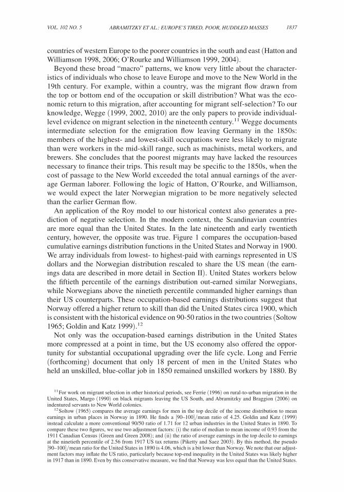
Notes: US and Norwegian distributions contain all men aged 38 to 50 in the respective censuses of 1900. The x-axis is scaled in 1900 US dollars. Individuals are assigned the mean earnings for their occupation and are arrayed from lowest- to highest-paid occupations. The Norwegian distribution is rescaled to have the same mean as the US distri-bution (the actual Norwegian and US means are US$(1900)350 and US$(1900)643, respectively).


Work on contemporary immigrant flows has found only mixed support for the Borjas model of migrant selection. Gould and Moav (2010) show that Israeli migrants to the United States are positively selected, at least on observable skills, as would be predicted by the more compressed distribution of Israeli wages.7 Chiquiar and Hanson (2005), however, observe that Mexican migrants to the United States are drawn from the middle, rather than the low end, of the Mexican skill distribution, despite the fact that income inequality is higher in Mexico than in the United States.8 Moreover, Feliciano (2005) and Grogger and Hanson (2008) find that migrants are selected positively on educational attainment from almost every sending country in the world, even those countries with very high levels of income inequality.

Scholars have attempted to reconcile the Borjas model with the facts about positive selection in a variety of ways. A new generation of models incorporates borrowing constraints and shows that, as the cost of migration increases, the poor-est residents of sending countries can no longer afford to move (Borger 2010; McKenzie and Rapoport 2010).9 Alternatively, Grogger and Hanson (2008) dem-onstrate that a classic Roy model with a linear, rather than a logarithmic, utility function generates predictions of positive selection whenever the skill-related dif-ferences in wage levels, rather than the relative return to skill in percentage terms, are high. In this framework, positive selection is a likely outcome in the contem-porary world given the dramatic difference in wage levels between developed and developing countries.

B. The Age of Mass Migration

Between 1850 and 1913, more than 40 million Europeans moved to the New World, nearly two-thirds of whom settled in the United States. Initially, migrants from the British Isles and Germany constituted the majority of the migrant flow to the United States. These early migrants were joined by Scandinavians and other northern Europeans in the 1870s and by southern and eastern Europeans in the 1880s. Norway experienced one of the highest out-migration rates in the 1880s, during which time 1 of every 100 Norwegians left the country on an annual basis.10

With the shift from sail to steam technology on the Atlantic, the cost of migration fell dramatically over the nineteenth century (Keeling 1999). The declining cost of migration, coupled with rising real incomes in the newly industrializing European periphery, relaxed the financial constraints on households that had previously been too poor to pay for passage to the New World. As migration became affordable to a greater share of the European population, the migrant flow shifted from the richer

7 See also Abramitzky (2009) and Borjas (2008), which find support for the Borjas selection hypothesis in the contexts of migration to and from Israeli kibbutzim and Puerto Rico, respectively.

8 See also a series of papers on migration from the Pacific Islands (Akee 2010; McKenzie, Gibson, and Stillman 2010; McKenzie and Gibson 2011).

9 According to data from the Mexican Migration Project, the median fee for being smuggled from Mexico into the United States is around US$(2000)2,000, or 35 percent of the annual earnings of a low-skilled Mexican worker (Borger 2010). This is a lower bound on the full cost of migration, which also includes forgone earnings and the expense of setting up a new household. Assuming that migrants lose around one month of work time during the journey and resettlement period, the full cost of migration may be closer to 50 percent of annual earnings.

10 This paragraph is based on Hatton and Williamson (1994, 1998).


countries of western Europe to the poorer countries in the south and east (Hatton and Williamson 1998, 2006; O’Rourke and Williamson 1999, 2004).

Beyond these broad “macro” patterns, we know very little about the character-istics of individuals who chose to leave Europe and move to the New World in the 19th century. For example, within a country, was the migrant flow drawn from the top or bottom end of the occupation or skill distribution? What was the eco-nomic return to this migration, after accounting for migrant self-selection? To our knowledge, Wegge (1999, 2002, 2010) are the only papers to provide individual-level evidence on migrant selection in the nineteenth century.11 Wegge documents intermediate selection for the emigration flow leaving Germany in the 1850s: members of the highest- and lowest-skill occupations were less likely to migrate than were workers in the mid-skill range, such as machinists, metal workers, and brewers. She concludes that the poorest migrants may have lacked the resources necessary to finance their trips. This result may be specific to the 1850s, when the cost of passage to the New World exceeded the total annual earnings of the aver-age German laborer. Following the logic of Hatton, O’Rourke, and Williamson, we would expect the later Norwegian migration to be more negatively selected than the earlier German flow.

An application of the Roy model to our historical context also generates a pre-diction of negative selection. In the modern context, the Scandinavian countries are more equal than the United States. In the late nineteenth and early twentieth century, however, the opposite was true. Figure 1 compares the occupation-based cumulative earnings distribution functions in the United States and Norway in 1900. We array individuals from lowest- to highest-paid with earnings represented in US dollars and the Norwegian distribution rescaled to share the US mean (the earn-ings data are described in more detail in Section II). United States workers below the fiftieth percentile of the earnings distribution out-earned similar Norwegians, while Norwegians above the ninetieth percentile commanded higher earnings than their US counterparts. These occupation-based earnings distributions suggest that Norway offered a higher return to skill than did the United States circa 1900, which is consistent with the historical evidence on 90-50 ratios in the two countries (Soltow 1965; Goldin and Katz 1999).12

Not only was the occupation-based earnings distribution in the United States more compressed at a point in time, but the US economy also offered the oppor-tunity for substantial occupational upgrading over the life cycle. Long and Ferrie (forthcoming) document that only 18 percent of men in the United States who held an unskilled, blue-collar job in 1850 remained unskilled workers by 1880. By

11 For work on migrant selection in other historical periods, see Ferrie (1996) on rural-to-urban migration in the United States, Margo (1990) on black migrants leaving the US South, and Abramitzky and Braggion (2006) on indentured servants to New World colonies.

12 Soltow (1965) compares the average earnings for men in the top decile of the income distribution to mean earnings in urban places in Norway in 1890. He finds a [90–100]/mean ratio of 4.25. Goldin and Katz (1999) instead calculate a more conventional 90/50 ratio of 1.71 for 12 urban industries in the United States in 1890. To compare these two figures, we use two adjustment factors: (i) the ratio of median to mean income of 0.93 from the 1911 Canadian Census (Green and Green 2008); and (ii) the ratio of average earnings in the top decile to earnings at the ninetieth percentile of 2.56 from 1917 US tax returns (Piketty and Saez 2003). By this method, the pseudo [90–100]/mean ratio for the United States in 1890 is 4.06, which is a bit lower than Norway. We note that our adjust-ment factors may inflate the US ratio, particularly because top-end inequality in the United States was likely higher in 1917 than in 1890. Even by this conservative measure, we find that Norway was less equal than the United States.


comparison, 47 percent of men in unskilled, blue-collar occupations in Norway in 1875 remained unskilled workers in 1900.13 Men who started their careers in unskilled occupations were twice as likely to move up the occupational ladder in the United States than in Norway over their lifetimes; much of this mobility was accomplished by moving into owner-occupier farming.

In historical terms, the costs of migration were relatively low in the late nineteenth century. We estimate that the total cost of migration, including forgone earnings dur-ing the voyage, represents around 18 percent of the annual earnings of a Norwegian farm laborer.14 Migrant networks also helped to defray the cost of passage for new arrivals; 40 percent of Norwegian migrants during this period travelled on prepaid steamship tickets financed by friends or relatives (Hvidt 1975).

II. Data and Matching

A. Matching Norwegian-Born Men to Their Birth Families

Our goal is to create a dataset of Norwegian migrants and nonmigrants whom we can observe both when living in their childhood households and when partici-pating in the labor market later in life. We rely on three census sources: the com-plete digitized Norwegian censuses of 1865 and 1900 (North Atlantic Population Project and Minnesota Population Center 2008), and a newly assembled dataset containing the full population of Norwegian-born men in the United States in 1900 (Ancestry.com). We use a standard iterative matching technique to match the popu-lation of Norwegian-born men in 1900 to their childhood households in 1865. This procedure (“Match 1”), which is described in more detail in Sections I and II of the online Appendix, generates a sample of 2,613 migrants and 17,833 nonmigrants.

Our baseline matching procedure uses only name, age, and country of birth to compare individuals across censuses. We can double our sample size by adding province of birth as a third match criterion for men who remain in Norway in 1900. This approach (“Match 2”), however, may introduce a bias by using different match-ing procedures for migrants and stayers. As a robustness exercise, we also match a restricted sample of men who are unique by name within a five-year age band in both censuses (two years around the reported age in each direction). This proce-dure (“Match 3”) limits the potential for false matches in 1900 but also reduces the sample size to 9,423.

B. Occupation and Earnings Data in Norway and the United States

We observe labor market outcomes in the year 1900, when the men in our sample were in their 30s and 40s. Neither the US nor the Norwegian census of 1900 con-tains individual information on wages or income in that year. Instead, we assign

13 We derive this result by matching men between the 1875 and 1900 Norwegian censuses using the matching procedure outlined in Section IIIA.

14 Norwegian farm laborers earned around US$(1900)175. For this calculation, we assume that migrants lost 20 days of work for the passage and the resettlement. It is interesting to note, however, that Armstrong and Lewis (2009) report that the typical Dutch migrant to Canada in the 1920s saved around US$(1900)150 for the cost of the voyage and resettlement, nearly a full year’s salary for a Norwegian farm laborer.

Ancestry.com


men the mean (PPP-adjusted) income earned by members of their occupation based either on the US 1901 Cost of Living survey (Preston and Haines 1991) or on tabulations published by Statistics Norway (Statistik Centralbureau 1905). Section III of the online Appendix describes these sources in more detail, while Section IV of the online Appendix presents our earnings estimates for farmers and fishermen, two occupations that are not included in the primary sources.

Our unavoidable reliance on mean earnings by occupation prevents us from mea-suring the full return to migration. Conceptually, the return to migration derives from three channels: (i) the presence of higher wages in the United States in the typ-ical occupation; (ii) the possibility that migrants are able to switch from low-paying to high-paying occupations upon arriving in the United States; and (iii) the potential for higher within-occupation return to ability in the United States. Our estimate of the return to migration cannot capture the third aspect of the total return because we do not observe variation in earnings within an occupation.

We face a related limitation in our ability to describe the extent of migrant selec-tion. Positive selection, for instance, could be generated either by high migration rates among men from occupations with high mean earnings or by high migration rates among men at the 80th or 90th percentiles of the wage distribution within their occupation. The reverse is true, of course, for negative selection. With our data, we can document the fact that more (fewer) common laborers moved to the United States, but we will not be able to observe whether the best (worst) among the labor-ers made the journey. Throughout the paper, we refer to this aspect of migration selection as “occupational selection.”

C. Comparing Matched Samples with the Full Population

Our matched samples may not be fully representative of the population of Norwegian-born men, either in 1865 or in 1900. In particular, matched samples are selected for having uncommon first and last names, which may have been associated with higher socioeconomic status. Section V of the online Appendix compares our matched sample to the population in 1865 and 1900. Men in the matched sample are demographically similar to the population in terms of age, number of siblings, and birth order. Perhaps because of the selection on having an uncommon name, how-ever, matched men are more likely to live in urban areas, both in childhood and as adults, and to hail from households of somewhat higher socioeconomic status than the population average. By adulthood, this privilege translates into slightly higher labor market earnings.

Although our matched sample is not fully representative of the population from which it is drawn, three things are worth noting. First, the direction and extent of this bias is nearly identical both for migrants and stayers. Therefore, the distinctive features of our matched sample are not likely to affect our estimates of the eco-nomic return to migration or our conclusions about migrant selection, which depend on a comparison of matched migrants to matched stayers rather than a compari-son of the matched sample to the population. Second, the main difference between our matched sample and the population is on urban status; therefore, throughout the paper we conduct our analysis separately for men hailing from urban and rural areas. Finally, to further reduce the differences between our matched sample and the


general population, we consider specifications that reweight our matched sample to resemble the frequencies of the following characteristics in the general population: urban residence (full sample only), asset holdings, and above-median occupation of the household head.

We address a few additional limitations of our matching procedure here. First, our matching procedure will not capture migrants who anglicize their names upon arrival in the United States, which could be a concern if changing one’s name is correlated with economic success. Following Fryer and Levitt (2004), we use the complete 1880 US census to construct indices of a name’s distinctively Norwegian content.15 By this metric, we find that men in our matched sample are no more likely than the typical migrant to have a distinctively Norwegian name (see online Appendix Table 7, row 7).16 In addition, we find no evidence that the “Norwegian-ness” of a man’s name is related to our occupation-based earnings measure.17

Second, our sample of matched migrants will not include temporary movers who returned to Norway before 1900. According to the aggregate statistics, 25 percent of the Norwegian migration flow eventually returned to Norway (Semmingsen 1978).18 Return migrants may have been drawn disproportionately from the upper or lower end of the occupational distribution, either because unsuccess-ful migrants return home to lean on their familial support network or because the most successful migrants are able to build up a certain level of savings most quickly in order to return home. The availability of an intermediate US census in 1880 allows us to address this point. We identify over 25,000 Norwegian-born men in the relevant age range in the 1880 census. We are able to locate 14 percent of these men in either the US or the Norwegian censuses of 1900; one-third of these had returned to Norway. We compare the economic outcomes of migrants who eventually returned to Norway and those who remained in the United States in 1880, when both sets of migrants were still living in the United States. Figure 2 reveals few discernible differences in the occupational distributions of these two groups.19 Men who eventually returned to Norway are slightly overrepresented at the bottom end of the occupational distribution, but the mean occupation scores of returners and persisters are statistically indistinguishable.

15 Our name index ranges from zero to two, with a value of zero reflecting the fact that no men in the United States with a given first and last name were born in Norway, and a value of two assigned to men whose first and last names are both distinctively Norwegian. The first name index is equal to

Pr[ 1 st name|Norwegian_born] ____

Pr[ 1 st name|Norw_born] + Pr[ 1 st name|not_Norw_born]

and likewise for the last name index. The full measure adds these two indices together.16 This pattern likely reflects a tradeoff: although we fail to match men who adopt less Norwegian names in the

United States, our matching procedure initially selects for men who have uncommon names (that is, names that are rare in Norway).

17 We regress ln(earnings) on the full name index and a quadratic for age for Norwegian-born men in the 1900 Integrated Public Use Microdata Series (IPUMS) in the relevant age range. The coefficient on the name index is 0.018 (standard error = 0.017). By this estimate, the average difference in the index value of 0.05 between matched and unmatched men would translate into a 0.1 percent difference in earnings, which is both small and statistically insignificant.

18 The United States only began tracking return migration in 1907–1908. Gould (1980) reports a much lower return migration rate (6.7 percent) for Norwegians for the 1907–1913 period.

19 We compare these groups using the occupation score variable available in the 1880 IPUMS data, rather than our occupation-based earnings measure. The occupation score variable is constructed in a similar manner by match-ing occupations to their median earnings in 1950.


D. The Occupational Distribution of Migrants versus Stayers

This section compares the occupational distributions of Norwegian migrants to the United States and men who remained in Norway in 1900. Table 1 reports the ten most common occupations for our sample of matched migrants in the United States and matched stayers in Norway. Although 40 percent of both groups report work-ing in farm occupations, migrants to the United States were much more likely to be owner-occupier farmers (36 percent versus 22 percent). Migrants were also more likely to report being general laborers (8 percent versus 1.4 percent). Other common occupations in both countries include carpenters, fishermen, and sailors.20

20 We also use the IPUMS and Norwegian census samples to compare the household composition of Norwegian migrants and stayers. Migrants are 7.6 percentage points less likely than men who remain in Norway ever to be married (coefficient = −0.076; standard error = 0.014). Conditional on ever being married, Norwegian migrants have around 0.5 more children than their nonmigrant counterparts (coefficient = 0.441, standard error = 0.111), perhaps because they have higher lifetime income. Given that migrants are less likely to marry, however, the average Norwegian migrant to the United States has no more children than does the average man in Norway.

0

0.02

0.04

0.06

Rel

ativ

e fr

eque

ncy

0 10 20 30 40

Earnings rank of occupation

US Norway

Figure 2. Comparing the Occupational Distributions of Migrants Who Stay in the United States or Return to Norway between 1880 and 1900

NMean occupation

score (1880)Percentage with

occupation score < 12

Unmatched 21,949 14.68 35.20Matched 3,597 14.65 36.50 Matched (US) 2,392 14.77 35.50 Matched (Norway) 1,205 14.39 38.40*

Notes: Return migrants are defined as Norwegian-born men observed in the 1880 US census who are matched to the 1900 Norwegian census (N = 1,205). Persistent migrants are Norwegian-born men in the US census of 1880 who are matched to the 1900 US census (N = 2,392). For comparison, unmatched men are Norwegian-born men in the 1880 US census who cannot be matched to either Norway or the United States in 1900. The occupation score measure, which is taken from the 1880 IPUMS sample, is constructed by ordering occupations according to their median earnings in 1950. The mean occupation score and share of the sample with an occupation score in the bottom quartile (score < 12) are reported in the accompanying table. On both measures, the differences between matched and unmatched men are not statistically significant. We mark differences between return and persistent migrants that are statistically different at the 10 percent level with an *.


Figure 3 presents the occupational distributions of these migrants and stayers, with occupations arrayed from lowest- to highest-paid according to the average US earnings in that occupation.21 We omit farmers, the largest occupational category, for reasons of scale, but results are qualitatively similar when farmers are included. For men born in urban areas, migrants are more likely to hold low-paying jobs such as day laborer or servant, while the men remaining in Norway exhibit an occupa-tion distribution that is skewed toward higher-paying jobs (for example, merchants). Men born in rural areas are employed in similar jobs in both countries.

When we impose the same mean earnings by occupation in Norway and the United States, we find that, on average, migrants from urban areas hold occupations that pay 19 log points less than those held by the typical man from an urban back-ground in Norway. Rural migrants also hold lower paying occupations although this gap is not as large (five log points). This negative “return to migration” is consistent

21 Chiquiar and Hanson (2005) conduct a similar exercise for Mexican migrants to the United States using the 2000 census. They assign migrants the earnings that they would have received, given their education and experience level, if they had remained in Mexico. Patterns are qualitatively similar when we use Norwegian earnings to create a common occupational ranking. We present results using US earnings here simply because the US earnings data are richer, reflecting nearly 200 occupational categories.

Table 1—Common Occupations Held by Norwegian-Born Men in the United States and Norway

Panel A. Top ten occupations in matched sample, Norwegian-born men living in the United States in 1900

Rank Occupation Frequency Percentage Earnings

1 Farmers and planters 1,012 35.81 6912 Laborers (general) 256 9.05 3733 Carpenters and joiners 174 6.15 6304 Farm laborers 101 3.57 2555 Painters, glaziers, and varnishers 66 2.33 6246 Sailors 60 2.12 4677 Saw and planing mill workers 42 1.49 5728 Machinists 39 1.38 7369 Railroad laborers 36 1.27 460

10 Salesmen 32 1.13 680Total 1,818 64.33

Notes: N = 2,826. Occupation data collected by hand from census manuscripts on Ancestry.com. Annual earnings by occupation data from the 1901 Cost of Living Survey reported in Preston and Haines (1991) in year 1900 dollars. Average income of owner-occupier farmers is estimated using data from the US census of agriculture.

Panel B. Top ten occupations in matched sample, Norwegian-born men living in Norway in 1900Rank Occupation Frequency Percentage Earnings

1 General farmers 4,189 22.26 3932 Farmer and fisherman 1,522 8.09 3213 Merchants and dealers 722 3.84 8374 Fisherman 709 3.77 2485 Husbandmen or cottars 658 3.50 1146 Farm workers 597 3.17 1757 Carpenters 505 2.68 3128 Shipmasters and captains 459 2.44 2989 Cottar and fisherman 412 2.19 321

10 Seamen 351 1.87 182Total 10,124 53.79

Notes: N = 18,820. Historical International Standard Classification of Occupations (HISCO) occupation catego-ries. Annual earnings by occupation data from Statistik Centralbureau (1905) and Grytten (2007). Values reported in year 1900 dollars. Average incomes of owner-occupier farmers and fishermen are estimated using data from the Norwegian census of agriculture.

Ancestry.com


with either initial negative occupational selection or occupational downgrading in the United States or both.22 We find similarly negative “returns to migration” for

22 Norwegian migrants may have experienced occupational upgrading or downgrading in the United States for various reasons. On the one hand, higher rates of occupational mobility in the United States may have allowed migrants to climb the occupational ladder. In particular, given the low price of land in the United States, many workers who started out as agricultural laborers were able to purchase their own farms and become owner-occu-piers. On the other hand, though, migrants may have lacked the US-specific skills necessary to secure highly paid occupations.

Panel A. Born in rural areas

Panel B. Born in urban areas

0.004

0.006

0.008

0.01

0.012

0.014

Rel

ativ

e fr

eque

ncy

0 50 100 150Occupation rank

0

0.005

0.01

0.015

Rel

ativ

e fr

eque

ncy

0 50 100 150Occupation rank

US Norway

Coefficient: –0.188Standard error: (0.016)

Coefficient: –0.058Standard error: (0.014)

US Norway

Figure 3. Comparing the Occupational Distributions of Norwegian-Born Men in the United States and Norway In 1900

Notes: Each figure presents the relative frequency of 144 earning categories (representing 189 distinct occupations) for Norwegian-born men in the United States and in Norway. All men are assigned the mean US earnings in their occupation. Men are divided by rural or urban place of birth. Farmers, the largest occupational category, is excluded from the figure for reasons of scale. We report coefficients and standard errors from OLS regressions of ln(earnings) on a dummy for living in the United States controlling for a quadratic in age.


migrants who have been in the United States for 20 years or more, however, which suggests against the possibility of temporary occupational downgrading. We would expect that the initial disadvantages that encourage migrants to take lower-skilled jobs upon first arrival in the country would erode over time as these migrants learn English and invest in other US-specific skills.

III. Estimating the Return to Migration in the Presence of Selection

A. Naïve Estimate of the Return to Migration: Mean Earnings of Migrants versus Stayers

One naïve approach to estimating the return to migration is to compare the occu-pation-based earnings of all Norwegian-born men living in the United States to all men in Norway in 1900:

(1) ln(Earning s i ) = α + β 1 (Migran t i ) + β 2 (Ag e i ) + β 3 (Ag e i 2 ) + ε i ,

where Earningsi denotes the mean earnings of members of individual i’s occupation in 1900 in his country of residence, Migranti is a dummy variable equal to one if individual i lives in the United States in 1900, and Agei and Agei

2 are individual i’s age and age-squared in 1900.23 The US census data are taken from IPUMS.24 For now, we measure the return to migration with β 1 , which measures the difference in the earnings of migrants and nonmigrants, adjusted for differences in the age profile.

We estimate equation (1) from a sample combining all Norwegian-born men between the ages of 38 and 50 from the 100 percent 1900 Norwegian census and the 1 percent sample of the 1900 US census.25 The first column of Table 2 shows that Norwegian migrants to the United States earned 61 log points (84 percent) more than men living in Norway in 1900. Columns 2 through 4 reproduce the OLS estimates from equation (1) in our three matched samples. The implied return to migration in our matched samples ranges from 57 to 64 log points (76 to 89 percent). The popula-tion estimate represents the midpoint of this range. The fifth column reweights our matched sample to reflect the urban status, asset holdings, and occupational distribu-tion of fathers in the full population, with little qualitative effect on the results.

In column 6, we assign US migrants the average earnings for their occupation from the 1915 Iowa census (appropriately deflated), which is more representative of the urban/rural composition of Norwegian migrants, resulting in a lower return to migra-tion of 55 log points (73 percent). The data from the Iowa census is described in more detail in the online Appendix, Section III. The seventh column builds in the 13 log point wage penalty experienced by Scandinavian migrants in the US labor market. We calculate the wage gap between Scandinavian migrants and native-born workers

23 Eighty-nine percent of men have a recorded occupation in the US or Norwegian census. In our main matched sample, missing occupation data reduces our sample from 19,970 to 17,758.

24 We also try using the “year of immigration” census variable to restrict our sample to men who were at least 18 years old at the time of immigration to exclude men who arrived in the United States as children. We find qualita-tively similar results for the regressions reported in Table 3 and all subsequent tables.

25 Although we estimate the earnings gap between the United States and Norway at a point in time, we note that the true return to migration is the net present value of potential earnings in the destination country relative to the source over the life cycle.


in the United States circa 1900 using data from the Immigration Commission and the census.26 As expected in this case, the return to migration falls to 47 log points (60 percent). Taken together, these adjustments suggest that the baseline estimates may be overstated due to the native-born and urban bias of the earnings data.

Note also that we capture the return to migration at a specific point, after three decades of United States-to-Norway migration. Ultimately, one could expect wages in the two countries to converge as out-migration reduced the labor supply in the sending country (O’Rourke and Williamson 1995, 1999, 2004). As a result, the return to migration would likely fall over time as the two countries experienced wage convergence.

B. Comparing Migrant and Nonmigrant Brothers within Households

The return to migration estimated in equation (1), β 1 , would be the true return if migrants were selected randomly from the Norwegian population. If, however, migrants are (positively or negatively) self-selected, then β 1 will be biased. We next

26 According to the Immigration Commission, Scandinavian migrants earned 15 log points below native-born workers in the same industry (Hatton and Williamson 1998). This wage penalty reflects not only the fact that, within industries, migrants may have held lower-paying occupations but also that migrants may have earned less than natives even within a given occupation. Using supplemental census data, we infer that the majority of this earnings penalty (13 log points) was due to within-occupation differences in wages. In particular, we use the 1900 IPUMS sample to run a regression of our (log) occupation-based earnings measure on being born in Scandinavia and industry fixed effects for the 16 narrowly defined mining and manufacturing industries reported in the Immigration Commission data. The Scandinavia coefficient is −0.018 ( p-value = 0.102), leading us to conclude that all but 2 log points of the 15-point wage penalty appears to have been due to within-occupation differences in wages. We note that some portion of the 13 log-point wage gap could be due to the fact that migrants are negatively selected. That is, perhaps migrants’ earnings would have been in the lower tail of the wage distribution in their occupation regardless of whether they lived in Norway or the United States. In this case, we would not want to adjust the return to migration for (all of) this 13 log-point wage gap. As a result, we choose not to highlight this specification as our preferred estimate of the return to migration.

Table 2—OLS Regressions of the Return to Migration from Norway to the United States

Dependent variable = ln(earnings)

Match 1Population Match 1 Match 2 Match 3 Weighted Iowa data Add penalty

(1) (2) (3) (4) (5) (6) (7)In US 0.609 0.606 0.644 0.572 0.641 0.554 0.466

(0.017) (0.009) (0.009) (0.015) (0.024) (0.010) (0.009)N 122,620 17,501 33,641 7,596 14,647 17,352 17,501

Notes: Standard errors are reported in parentheses. All regressions control a quadratic in age. The first column con-tains a representative sample of the population of Norwegian-born men between the ages of 38–50 in 1900 from the 100 percent 1900 Norwegian census and 1 percent 1900 US census sample (IPUMS). Column 2 reports estimates from the first matched sample, which is based on an iterative matching strategy that searches first for an exact match and then for matches in a one- or two-year age band. Column 3 uses the second matched sample, which allows men to match in Norway by name, age, and province of birth. Column 4 reports estimates from the third matched sam-ple, which instead requires that matched observations be unique within a five-year age band. Columns 5 through 7 return to the first matched sample. In column 5, US migrants are assigned earnings from the 1915 Iowa census (appropriately adjusted for inflation). We lose 157 observations whose occupations do not match categories in the Iowa census. In column 6, we reduce the Cost of Living earnings by 13 log points in each occupation based on the earnings penalty for Scandinavian migrants reported in Hatton and Williamson (1994). Column 7 weights the matched sample to reflect the urban status, asset holdings and occupational distribution of fathers in the full popula-tion. We lose 2,905 observations because of missing information (primarily missing data on fathers’ occupations).


compare the occupation-based earnings of migrants and their nonmigrant brothers to eliminate selection across households. Such selection occurs if men from richer or poorer households are more likely migrate to the United States.

We consider the following equation in which the individual error term is decom-posed into two components:

(2) ln(Earning s ij ) = β 1 ′ (Migran t ij ) + β 2 ′ (Ag e ij ) + β 3 ′ (Ag e ij 2 ) + α j + ν ij ,

where α j is the component of the error that is shared between brothers in the same household j and ν ij is the component that is idiosyncratic to individuals.

Running an OLS regression of equation (2) with household fixed effects will absorb the fixed household portion of the error term ( α j ). Such within-household estimation will eliminate bias due to aspects of family background that are corre-lated both with the probability of migration and with labor market outcomes later in life.27 In this case, the coefficient β 1 ′ measures the return to migration, free from selection across households.

Table 3 compares the naïve OLS and within-household estimates of the return to migration. In order to contribute to the within-household estimation, a household must contain at least two members who match between 1865 and 1900. We begin in the first row of each panel by conducting OLS on the subsample of households with two or more matched members (including migrant-stayer, migrant-migrant, and stayer-stayer pairs). The unweighted return to migration is 55 log points (73 per-cent), which is a weighted average of 61 log points (84 percent) for men born in rural areas and only 39 log points (48 percent) for men born in urban areas.28 The second row in each panel adds household fixed effects. In both weighted and unweighted specifications, we find that adding household fixed effects reduces the estimated return to migration (relative to OLS) in the rural sample and increases the estimated return to migration in the urban sample. The differences between the coefficients are statistically significant in both regions.

By comparing the naïve OLS estimate of the return to migration ( β 1 ) and the within-household OLS estimate ( β 1 ′ ), we can infer the direction and magnitude of occupational selection across households. Specifically, if β 1 ′ > β 1 , it would suggest that β 1 was biased downward by negative selection of migrant households. That is, men from the types of households that send migrants to the United States would have had low earnings even if they stayed in Norway. In contrast, if β 1 ′ < β 1 , it would suggest that β 1 was biased upward by positive selection of migrant households.

By this method, we find evidence of negative occupational selection across house-holds for migrants leaving urban areas (that is, β 1 ′ > β 1 ). In particular, the return to migration estimates increase by 22 to 30 percent with the inclusion of household fixed effects. In contrast, the within-household estimates are smaller than their OLS counterparts (13 to 15 percent) in the rural sample. Overall, this method provides

27 See Griliches (1979), Altonji and Dunn (1996), Aaronson (1998), and Sacerdote (2007) for examples of within-sibling estimates in other contexts. Ashenfelter and Krueger (1994), Behrman, Rosenzweig, and Taubman (1996), and Behrman and Rosenzweig (2002) use pairs of identical twins to estimate the returns to schooling.

28 The return to migration in this subsample is somewhat lower than in the matched samples as a whole (Table 3), perhaps because households with two matched members are more likely to have a high socioeconomic status.


evidence that the migrant flow from Norwegian cities and towns was drawn from households from a lower occupational stratum and that migrants from rural areas were positively selected.

C. Individual-level Instruments for Migration

Even within households, brothers can differ in unmeasured personal attributes (denoted as ν ij in equation (2)). Appendix A provides complementary evidence on the return to migration and migrant selection using the gender composition of a man’s siblings and his place in the household birth order to instrument for migra-tion. Both of these factors influence a man’s expectation of inheriting farmland in Norway and therefore his probability of migrating to the United States. The exclu-sion restrictions are that these two factors do not affect our measure of occupation-based earnings directly, and the Appendix provides supporting evidence that this was likely the case in our context.

We focus on the subsample of men born in rural areas whose childhood household held some assets in 1865. Conditional on the number of siblings in the household, the presence of an additional brother increases an individual’s probability of migrating to the United States by 1.6 percentage points (relative to the sample migration rate of 11.9 percent). Men who rank third or higher in the son order are around 5 percentage

Table 3 —Ols and Within-Household Estimates of the Return to Migration. Households with Two or More Members in the Matched Sample

Dependent variable = ln(earnings); Coefficient on = 1 if migrantFull sample, 1865 Rural, 1865 Urban, 1865

Panel A. UnweightedOLS 0.545 0.607 0.384

(0.027) (0.034) (0.044)Within household 0.511 0.508 0.508

(0.035) (0.045) (0.057)Chi-squared 1.49 7.47 8.31p-value 0.2218 0.0063 0.0039N 2,655 1,823 832Number of migrant-stayer pairs 326 167 159

Panel B. WeightedOLS 0.586 0.609 0.443

(0.029) (0.033) (0.067)Within household 0.542 0.529 0.561

(0.039) (0.042) (0.049)Chi-squared 2.13 4.60 5.65p-value 0.1441 0.0320 0.0175N 2,241 1,666 306Number of migrant-stayer pairs 269 140 129

Notes: Each cell contains coefficient estimates and standard errors from regressions of ln(earnings) on a dummy variable equal to one for individuals living in the United States in 1900. Regressions also include controls for age and age squared. In each panel, the first row conducts an OLS regression for the restricted sample of households that have at least two matched members in the dataset and the second row adds household fixed effects. Panel B contains results from regressions weighted to reflect the urban status (full sample only), asset holdings, and occupational distribution of fathers in the full population. We conduct chi-squared tests of the null hypothesis that the OLS and within-household coefficients are equal.


points more likely to migrate than their older brothers.29 The OLS estimate of the return to migration for this selected sample is 64 log points (90 percent). Our IV esti-mates range from 67 to 70 log points (95 to 101 percent). The larger IV coefficient suggests that the simple earnings comparison may be biased downward, a pattern that is consistent with negative occupational selection in this rural subsample.

IV. Additional Evidence of Migrant Selection: Fathers’ Earnings and Wealth

Thus far, we have inferred the direction of migrant selection by comparing naïve estimates of the return to migration with estimates that eliminate across-household selection. In this section, we provide additional evidence on migrant selection by comparing the economic outcomes of the fathers of migrants and stayers in the 1865 Norwegian census and the 1886 Land Registers (Norwegian Historical Data Centre 2010). Focusing on fathers’ outcomes has two advantages. First, fathers’ outcomes are all measured in the same economic environment. Second, fathers’ outcomes are predetermined and not affected by the migration decision.

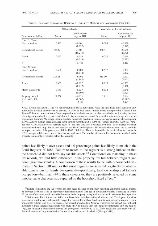
Table 4 compares the occupations, asset holdings, and property tax values of the heads of migrant and nonmigrant households in 1865. In particular, we regress each of these economic outcomes (Yjr) on an indicator for the migrant status of the household (MigrantHouseholdj), controlling for the age of the head of the house-hold (Agej, and Age 2j ) and a series of province dummies (δr):

(3) Y jr = γ 1 MigrantHousehol d j + γ 2 Ag e j + γ 3 Ag e j 2 + δ r + ε jr .

Households are placed in the “migrant” category if at least one son lived in the United States in 1900 and in the “nonmigrant” category otherwise. The first panel includes all households with at least one matched son. In the full sample, however, we may erroneously place true migrant households into the nonmigrant category because we cannot determine the migration status of unmatched sons. Therefore, in the second panel, we restrict our attention to households in which all sons are matched either to the United States or to Norway in 1900. In both cases, we find evidence of negative selection from urban and rural areas. That is, the heads of households that sent migrants to the United States were less likely to own assets and more likely to hold occupations with below-median average earnings.

As expected, the patterns are stronger when we focus on households in which the migration status of all sons is known. In the urban portion of this subsample, we find that the heads of migrant households are 5.8 percentage points less likely to own assets than the heads of nonmigrant households. In rural areas, heads of migrant households are 5.4 percentage points less likely to hold an occupation with above-median earnings. All of these contrasts are statistically significant at the 10 percent level. In addition, rural heads of migrant households are 3.5 percentage

29 We do not observe a difference in migration rates between the first- and second-born sons, suggesting either that inheritance practices may not have followed a strict form of primogeniture in this period or that second sons regularly replaced first sons who died or were otherwise incapacitated before the family property could change hands.


points less likely to own assets and 4.0 percentage points less likely to match to the Land Register of 1886. Failure to match to the register is a strong indication that the household did not have any taxable assets.30 Conditional on matching to these tax records, we find little difference in the property tax bill between migrant and nonmigrant households. A comparison of these results to the within-household esti-mates in Section IIIB implies that rural migrants are selected negatively on observ-able dimensions of family background—specifically, land ownership and father’s occupation—but that, within these categories, they are positively selected on some unobservable characteristic captured by the household fixed effect.31

30 Failure to match to the tax records can also occur because of imperfect matching conditions such as mortal-ity between 1865 and 1886 or improperly transcribed names. The age of the household head is missing in around 25 percent of the cases; we do not add this control in the property tax regression to maintain a reasonable sample size.

31 To illustrate this point, we subdivide rural households into those with and without land. The degree of positive selection in rural areas is substantially larger for households without land (results available upon request). Rural households without land were, on average, the poorest households in Norway. Therefore, we suspect that, although members of these landless households were more likely to migrate than their landed counterparts, only the best-off (e.g., less financially constrained) among this poor group were able to do so. These results are consistent with dif-ferential patterns of migrant selection from rural and urban areas in Mexico (Moraga 2011).

Table 4—Economic Outcomes of Household Heads with Migrant and Nonmigrant Sons, 1865

All households Households with matched sons

Dependent variables MeanCoefficient on migrant HH Mean

Coefficient on migrant HH

Panel A. UrbanOcc. > median 0.593 −0.001 0.583 −0.030

(0.022) (0.042)Occupational income 428.27 −27.501 440.47 −26.555

(10.216) (20.798)Assets 0.260 −0.030 0.252 −0.058

(0.018) (0.035)N 4,038 1,074

Panel B. RuralOcc. > median 0.608 0.008 0.577 −0.054

(0.014) (0.032)Occupational income 321.21 6.092 315.30 −9.077

(3.847) (9.072)Assets 0.665 −0.032 0.613 −0.035

(0.012) (0.028)Match tax records 0.130 −0.037 0.134 −0.040

(0.009) (0.021)Property tax bill 2.759 −0.372 2.821 0.044N = 1,410; 300 (0.307) (0.887)N 12,177 2,499

Notes: Results for Match 1. The left-hand panel includes all households while the right-hand panel considers only households in which all sons can be matched to 1900. In each panel, sample means are reported in Column 1 and the coefficient and standard error from a regression of each dependent variable on an indicator for being the head of a migrant household is reported in Column 2. Regressions also control for a quadratic in head’s age and a series of province dummies. We assign income levels to household heads using mean Norwegian earnings by occupation in 1900. Above-median occupations are those earning more than US$(1900)311 (urban) and US$(1900)393 (rural) per year. Assets is an indicator variable equal to 1 for men who own a business, own land, or are master craftsmen in an artisanal workshop. Tax records refers to the 1886 Land Registers. For fathers who match to the tax records, we report the value of the property tax bill in 1900 US dollars. The data is provided in speciedalers and marks. In 1875, one speciedaler was equal to four Norwegian kroner. The number of households that can be matched to the property tax records is reported below that variable.


V. Conclusion

We know surprisingly little about how migrants during the Age of Mass Migration were selected from the European population and about the economic return from their journey. In this paper, we construct a new dataset of Norwegian-to-United States migration to estimate the return to migration in the presence of selection into migration. We compare the occupation-based earnings of men who moved to the United States and their brothers who stayed behind in Norway. This approach eliminates the component of migrant selection that takes place across households. We gather further evidence about the nature of migrant selection by comparing the economic outcomes of fathers of migrants and nonmigrants.

We estimate a return to migration from Norway to the United States of around 70 percent, which is substantially smaller than the 200–400 percent return for migra-tion from Mexico to the United States today (Hanson 2006). The contemporary return to migration may be higher than in the past because of the sizeable cost of migration—both the bureaucratic costs of legal immigration and the cost of evading detection for the undocumented—which together reduce the supply of immigrants to the country. In the late nineteenth century, the border was open to almost all prospective migrants and, therefore, the return to migration was relatively low. We note, however, that the decision to migrate in the nineteenth century (as today) may have entailed other nonpecuniary considerations that would have increased the total return to migration (Bertocchi and Strozzi 2008). For example, at the time, Norway was under Swedish control and limited its franchise to men with wealth, while the United States offered the opportunity (for white men) to participate in the demo-cratic system even to new migrants.

We find mixed evidence on selection for rural migrants, with some methods sug-gesting positive selection and others suggesting negative selection. In contrast, we consistently find that men from urban areas who faced poor economic prospects in Norway, as measured by occupation, were more likely to migrate to the United States. One result of this negative occupational selection is that the naïve return to migration underestimates the true return by 20 to 30 percent for the urban sam-ple. The fact that migrants to the United States appear to have been drawn from the lower end of the occupational distribution is consistent with a standard Roy model of migration, as in Borjas (1987), which predicts that men at the lower end of the occupational distribution would have more to gain by moving from relatively unequal European countries to the New World. Furthermore, the fact that European migrants from urban areas, when unhindered by entry restrictions, were negatively selected from the sending population may explain why the United States eventually closed its border to the free flow of labor in 1924 (Hatton and Williamson 2006) and why some countries explicitly select for more skilled applicants in their immigration policies today.

Appendix A: IV Estimates

Comparing the within-household and naïve OLS estimates of the return to migra-tion reveals selection in the type of households that sent migrants to the United States. Even within households, however, brothers differ in unmeasured personal


attributes (denoted as ν ij in equation (2)). In this section, we turn to a complemen-tary instrumental variables estimation that can address both across- and within-household forms of selection. In particular, we aim to find individual characteristics that are correlated with the propensity to migrate but not otherwise associated with labor market potential.

One factor that may have influenced the decision to migrate was the expecta-tion of inheriting farmland in Norway. Historically, property was only passed to sons. Some regions of Norway also relied on a primogeniture system of inheritance wherein the eldest brother stood to inherit the family assets and the corresponding obligation to care for his aging parents. In this social context, younger brothers, who had to “make their own way” in the world, may have been more likely to migrate to the United States.32 In accordance with these historical inheritance practices, we consider two instruments for migration status: the gender composition of a man’s siblings and his place in the household birth order. Conditional on the number of siblings, men with fewer brothers received a larger share of the total inheritance. In areas that practiced primogeniture, elder brothers were more likely than younger brothers to inherit land (again, conditional on total number of siblings).

For the instrumental variable (IV) analysis, we focus on the subsample of men who were most likely to receive an inheritance in land, namely those who were born in rural areas and whose childhood household held some assets in 1865. Furthermore, to minimize measurement error in household composition, we limit our attention to men whose mothers were young enough for a (near-)complete household structure to be observed in 1865.33 Using this sample, we estimate the following first-stage equation:

(A1) Migran t ij = α + γ 1 (Brother s j ) + Γ 1 (Sibling s j )

+ Γ 2 (Ran k ij ) + γ 2 (Ag e i ) + γ 3 (Ag e i 2 ) + ε ij ,

where Migrantij is equal to 1 for individual i from household j living in the United States in 1900. The variables of interest are the number of brothers in the household (Brothersj) and an individual’s rank among these brothers (Rankij). We include both specifications that include both instruments and ones that use them separately. We also include dummy variables for the number of siblings in the household (Siblingsj) and control for a quadratic in age. We note that conditional on the number of siblings in the household, both the number of brothers and an individual’s place in the birth order of sons are random.

32 In his detailed social history of migration from western Norway, Gjerde (1985) argues that migration was one solution for younger siblings who were constrained by the “system of primogeniture … [under which] they could be nourished and remain on the farm, but they could not marry until they acquired livelihoods that would sustain new families” (p. 86). See Guinnane (1992) and Wegge (1999) for empirical work on the relationship between inheritance systems and immigration in other European contexts.

33 We restrict the sample to men whose mothers were 42 years old or younger in 1865. This cutoff was selected according to the following logic: (i) age at first birth was high in Norway during this period; in the 1865 Census, only 13 percent of women had a (surviving) child by the age of 23; (ii) furthermore, children lived with their parents until their late adolescence; 91 percent lived in their childhood until at least the age of 19. Together, these two facts imply that household structure would be incomplete for only 1.2 percent of 42-year old mothers in 1865 (= 0.13 with child by age 23 × 0.09 who left home by age 19). Our results are robust to increasing the age cutoff to 45.


The second stage of the IV specification is

(A2) ln(Earnings ) ij = α + γ 1 (Migran t ij ) + Γ 1 (Sibling s j )

+ γ 2 (Ag e i ) + γ 3 (Ag e i 2 ) + μ ij .

The independent variable of interest is Migrantij, which is instrumented with the number of brothers in the household Brothersj and/or with an individual’s rank among these brothers Rankij.

The identifying assumption underlying these instruments is that household com-position has no influence on labor market outcomes beyond its effect on the prob-ability of migration. Men who have few brothers or who are eldest among their brothers, however, may not only benefit directly from receiving an inheritance but may also be the beneficiaries of complementary human capital investments in child-hood.34 This possibility is not borne out in our data: among men who remain in Norway, we find no relationship between the composition of a man’s childhood household and his labor market outcomes in 1900. We estimated regressions of ln(earnings) on either number of brothers or birth order for the subsample of men who lived in Norway in 1900, controlling for number of siblings, age, and province of birth. We find no relationship between number of brothers and earnings (coef-ficient = 0.003, standard error = 0.008) and a statistically insignificant and positive relationship between being third or higher in the birth order of sons and earnings (coefficient = 0.021, standard error = 0.023).35

Our IV results are presented in Appendix Table A1. Panel A reports estimates from the first-stage equations. Conditional on the number of siblings in the house-hold, the presence of an additional brother increases an individual’s probability of migrating to the United States by 1.6 percentage points (relative to the sample migration rate of 11.9 percent). In the second column, we find that men who rank third, fourth, or higher in the son order are 5 to 8 percentage points more likely to migrate than their older brothers. We do not observe a difference in migration rates between the first and second born sons, however, suggesting either that inheritance practices may not have followed a strict form of primogeniture in this period or that second sons regularly replaced first sons who died or were otherwise incapacitated before the family property could change hands. Interestingly, in rural households without assets, men with more brothers or who are themselves further down the birth order are somewhat less likely to migrate (not shown), which we take as suggestive evidence that the effects of household composition estimated here operate through an inheritance channel.

Panels B and C, respectively, contain OLS and IV estimates of the return to migra-tion for the rural subsample (equation (4) above). The OLS estimate of the return to migration for this selected sample is 64 log points (90 percent). Our IV estimates in

34 On the role of sibling gender on human capital investments, see Butcher and Case (1994) and Garg and Morduch (1998). Black, Devereux, and Salvanes (2005) show that birth order affects labor market outcomes in the modern Norwegian economy.

35 We acknowledge that, because younger siblings are more likely to migrate to the United States, the selection of who remains in Norway may differ by birth order, thereby weakening the power of our test.


panel C range from 67 to 70 log points (95 to 101 percent). The larger IV coefficient suggests that the simple earnings comparison may be biased downward by a small amount, a pattern that is again consistent with mild negative selection of migrants from rural areas.36

REFERENCES

Aaronson, Daniel. 1998. “Using Sibling Data to Estimate the Impact of Neighborhoods on Children’s Educational Outcomes.” Journal of Human Resources 33 (4): 915–46.

Abramitzky, Ran. 2009. “The Effect of Redistribution on Migration: Evidence from the Israeli Kib-butz.” Journal of Public Economics 93 (3–4): 498–511.

Abramitzky, Ran, Leah Platt Boustan, and Katherine Eriksson. 2012. “Europe’s Tired, Poor, Huddled Masses: Self-Selection and Economic Outcomes in the Age of Mass Migration: Dataset.” American Economic Review. http://dx.doi.org/10.1257/aer.102.5.1832.

Abramitzky, Ran, and Fabio Braggion. 2006. “Migration and Human Capital: Self-Selection of Inden-tured Servants to the Americas.” Journal of Economic History 66 (4): 882–905.

Akee, Randall. 2010. “Who Leaves? Deciphering Immigrant Self-Selection from a Developing Coun-try.” Economic Development and Cultural Change 58 (2): 323–44.

Altonji, Joseph G., and Thomas A. Dunn. 1996. “Using Siblings to Estimate the Effect of School Qual-ity on Wages.” Review of Economics and Statistics 78 (4): 665–71.

Ancestry.com. “Genealogy, Family Trees and Family History Records online.” The Generations Net-work, Inc. http://www.ancestry.com/.

36 In the case of a discrete regressor, the measurement error is nonclassical. Therefore, the fact that the IV esti-mate is larger than OLS is not necessarily due to a correction for attenuation bias (see Cameron 2007).

Appendix Table A1—Birth Order and Number of Brothers as Instruments for Migration to the United States

(1) (2) (3)

Panel A. First stage Dependent variable = In US in 1900Number of brothers 0.016 0.011

(0.006) (0.006)2nd brother −0.000 —

(0.012)3rd brother 0.047 0.037

(0.019) (0.019)4th or higher brother 0.076 0.058

(0.035) (0.036)

Panel B. OLS Dependent variable = ln(earnings in 1900)In US in 1900 0.642

(0.019)

Panel C. IV Dependent variable = ln(earnings in 1900)In US in 1900 0.669 0.696 0.668

(0.436) (0.381) (0.338)Over-ID test (p-value) 0.869N 4031 4031 4031

Notes: Standard errors are reported in parentheses. The sample includes men in Match 1 who lived in a rural household that had some assets in 1865 and whose mother is 42 years old or younger in 1865. The regressions also include a quadratic in age and dummy variables for total number of siblings in the household (see equation (3) in the text). In column 3, we report the p-value from a Sargan (chi-squared) test of overidentification.


Ancestry.com

http://www.ancestry.com/


Armstrong, Alexander, and Frank Lewis. 2009. “Capital Constraints and European Migration to Can-ada: Evidence from the 1920s Passenger Lists.” Queen’s University, Department of Economics Working Paper 1230.

Ashenfelter, Orley, and Alan B. Krueger. 1994. “Estimates of the Economic Returns to Schooling from a New Sample of Twins.” American Economic Review 84 (5): 1157–73.

Atack, Jeremy, Fred Bateman, and Mary Eschelbach Gregson. 1992. “‘Matchmaker, Matchmaker, Make Me a Match’: A General Personal Computer-Based Matching Program for Historical Research.” Historical Methods 25 (2): 53–65.

Behrman, Jere R., and Mark R. Rosenzweig. 2002. “Does Increasing Women’s Schooling Raise the Schooling of the Next Generation?” American Economic Review 92 (1): 323 –34.

Behrman, Jere R., Mark Rosenzweig, and Paul Taubman. 1996. “College Choice and Wages: Esti-mates Using Data on Female Twins.” Review of Economics and Statistics 78 (4): 672–85.

Bertocchi, Graziella, and Chiara Strozzi. 2008. “International Migration and the Role of Institutions.” Public Choice 137 (1–2): 81–102.

Black, Sandra E., Paul J. Devereux, and Kjell G. Salvanes. 2005. “The More the Merrier? The Effect of Family Size and Birth Order on Children’s Education.” Quarterly Journal of Economics 120 (2): 669–700.

Borger, Scott. 2010. “Self-Selection and Liquidity Constraints in Different Migration Cost Regimes.” http://econ.ucsd.edu/~sborger/Constraint1.pdf (accessed March 1, 2011).

Borjas, George J. 1987. “Self-Selection and the Earnings of Immigrants.” American Economic Review 77 (4): 531–53.

Borjas, George J. 1991. “Immigration and Self-Selection.” In Immigration, Trade, and the Labor Mar-ket, edited by John M. Abowd and Richard B. Freeman, 29–76. Chicago: University of Chicago Press.

Borjas, George J. 2008. “Labor Outflows and Labor Inflows in Puerto Rico.” Journal of Human Capi-tal 2 (1): 32–68.

Butcher, Kristin F., and Anne Case. 1994. “The Effect of Sibling Sex Composition on Women’s Edu-cation and Earnings.” Quarterly Journal of Economics 109 (3): 531–63.

Cameron, A. Colin. 2009. “Microeconometrics: Current Methods and Some Recent Developments.” In Palgrave Handbook of Econometrics, edited by Terence C. Mills and Kerry Paterson, 729–74. New York: Palgrave MacMillan.

Chiquiar, Daniel, and Gordon H. Hanson. 2005. “International Migration, Self-Selection, and the Dis-tribution of Wages: Evidence from Mexico and the United States.” Journal of Political Economy 113 (2): 239–81.

Chiswick, Barry. 1999. “Are Immigrants Favorably Self-Selected?” American Economic Review 89 (2): 181–85.

Chiswick, Barry. 2000. “Are Immigrants Favorably Self-Selected? An Economic Analysis.” In Migra-tion Theory: Talking across Disciplines, edited by Caroline B. Brettell and James F. Hollifield, 61–76. New York: Routledge.

Feliciano, Cynthia. 2005. “Educational Selectivity in U.S. Immigration: How Do Immigrants Compare to Those Left Behind?” Demography 42 (1): 131–52.

Ferenczi, Imre, and Walter Willcox. 1929. International Migrations. New York: National Bureau of Economic Research.

Ferrie, Joseph. 1996. “A New Sample of Males Linked from the Public Use Micro Sample of the 1850 U.S. Federal Census of Population to the 1860 U.S. Federal Census Manuscript Schedules.” His-torical Methods 29: 141–56.

Fryer, Roland G., Jr., and Steven D. Levitt. 2004. “The Causes and Consequences of Distinctively Black Names.” Quarterly Journal of Economics 119 (3): 767–805.

Garg, Ashish, and Jonathan Morduch. 1998. “Sibling Rivalry and the Gender Gap: Evidence from Child Health Outcomes in Ghana.” Journal of Population Economics 11 (4): 471–93.

Gibson, John, and David McKenzie. 2011. “The Microeconomic Determinants of Emigration and Return Migration of the Best and Brightest: Evidence from the Pacific.” Journal of Development Economics 95 (1): 18–29.

Gjerde, Jon. 1985. From Peasants to Farmers: The Migration from Balestrand, Norway to the Upper Middle West. New York: Cambridge University Press.

Global Financial Data. “British Pound-Norway Krone Exchange Rate.” http://www. globalfinancial-data.com (accessed May 15, 2009).

Goldenweiser, E. A. 1916. “The Farmer’s Income.” American Economic Review 6 (1): 42–48.Goldin, Claudia, and Lawrence F. Katz. 1999. “The Returns to Skill in the United States across the

Twentieth Century.” National Bureau of Economic Research Working Paper 7126.Gould, Eric D., and Omer Moav. 2010. “When Is ‘Too Much’ Inequality Not Enough? The Selection

of Israeli Emigrants.” http://www.ecore.be/Papers/1280145355.pdf.

http://econ.ucsd.edu/~sborger/Constraint1.pdf

globalfinancialdata.com

globalfinancialdata.com

http://www.ecore.be/Papers/1280145355.pdf


Gould, J. D. 1980. “European Inter-Continental Emigration. The Road Home: Return Migration from the U.S.A.” Journal of European Economic History 9 (1): 41–112.

Green, Alan G., and David A. Green. 2008. “Immigration and Canada’s Wage Structure in the First Half of the Twentieth Century.” http://qed.econ.queensu.ca/CNEH/papers/GreenGreen.pdf.

Griliches, Zvi. 1979. “Sibling Models and Data in Economics: Beginnings of a Survey.” Journal of Political Economy 87 (5): S37–64.

Grogger, Jeffrey, and Gordon H. Hanson. 2008. “Income Maximization and the Selection and Sorting of International Migrants.” National Bureau of Economic Research Working Paper 13821.

Grytten, Ola H. 2004. “A Consumer Price Index for Norway, 1516-2003.” In Historical Monetary Sta-tistics for Norway, 1819–2003, edited by Øyvind Eitrheim, Jan T. Klovland, and Jan F. Qvigstad. Norges Banks Occasional Papers 35.

Grytten, Ola H. 2007. “Nominal Wages in Norway 1726–1940 by Occupation.” In Historical Mone-tary Statistics for Norway – Part II, edited by Øyvind Eitrheim, Jan T. Klovland, and Jan F. Qvigs-tad. Oslo, Norway: Norges Bank Oslo.

Guinnane, Timothy W. 1992. “Intergenerational Transfers, Emigration, and the Rural Irish Household System.” Explorations in Economic History 29 (4): 456–76.

Hanson, Gordon H. 2006. “Illegal Migration from Mexico to the United States.” Journal of Economic Literature 44 (4): 869–924.

Hatton, Timothy J., and Jeffrey G. Williamson. 1994. “What Drove the Mass Migrations from Europe in the Late Nineteenth Century?” Population and Development Review 20 (3): 533–59.

Hatton, Timothy J., and Jeffrey G. Williamson. 1998. The Age of Mass Migration: Causes and Eco-nomic Impact. New York: Oxford University Press.

Hatton, Timothy J., and Jeffrey G. Williamson. 2006. “International Migration in the Long Run: Posi-tive Selection, Negative Selection, and Policy.” In Labor Mobility and the World Economy, edited by Federico Foders and Rolf J. Langhammer, 1–31. New York: Springer.

Hvidt, Kristian. 1975. Flight to America: The Social Background of 300,000 Danish Immigrants. New York: Academic Press.

Keeling, Drew. 1999. “The Transportation Revolution and Transatlantic Migration, 1850-1914.” In Research in Economic History Volume 19, edited by Alexander J. Field, Gregory Clark, and William A. Sundstrom, 39–74. Stamford, CT: JAI Press.

Long, Jason, and Joseph Ferrie. Forthcoming. “Intergenerational Occupational Mobility in Britain and the US Since 1850.” American Economic Review.

Margo, Robert A. 1990. Race and Schooling in the South, 1880–1950: An Economic History. Chicago: University of Chicago Press.

McKenzie, David, John Gibson, and Steven Stillman. 2010. “How Important Is Selection? Experimen-tal vs. Non-experimental Measures of the Income Gains from Migration.” Journal of the European Economic Association 8 (4): 913–45.

McKenzie, David, and Hillel Rapoport. 2010. “Self-Selection Patterns in Mexico-U.S. Migration: The Role of Migration Networks.” Review of Economics and Statistics 92 (4): 811–21.

Mitchell, Wesley, Willford I. King, Frederick R. Macaulay, and Oswald W. Knauth. 1922. Income in the United States: Its Amount and Distribution, 1909–1919. New York: National Bureau of Eco-nomic Research.

Moraga, Jesús Fernández-Huertas. 2011. “New Evidence on Emigrant Selection.” Review of Econom-ics and Statistics 93 (1): 72–96.

North Atlantic Population Project and Minnesota Population Center. 2008. NAPP: Complete Count Microdata. NAPP Version 2.0 [computer files]. Minneapolis, MN: Minnesota Population Center. http://www.nappdata.org.

Norwegian Historical Data Centre. 2010. Land Registers 1886. [computer files]. Troms, Norway: Uni-versity of Troms.

O’Rourke, Kevin. 2004. “The Era of Free Migration: Lessons for Today.” IIIS Discussion Paper 18.O’Rourke, Kevin Hjortshoj, and Jeffrey G. Williamson. 1995. “Open Economy Forces and Late Nine-

teenth Century Swedish Catch-Up: A Quantitative Accounting.” Scandinavian Economic History Review 43 (2): 171–203.

O’Rourke, Kevin H., and Jeffrey G. Williamson. 1999. Globalization and History: The Evolution of a Nineteenth-Century Atlantic Economy. Cambridge, MA: MIT Press.

Piketty, Thomas, and Emmanuel Saez. 2003. “Income Inequality in the United States, 1913–1998.” Quarterly Journal of Economics 118 (1): 1–39.

Preston, Samuel H., and Michael R. Haines. 1991. Fatal Years: Child Mortality in Late Nineteenth-Century America. Princeton, NJ: Princeton University Press.

Roy, A. D. 1951. “Some Thoughts on the Distribution of Earnings.” Oxford Economic Papers New Series 3 (2): 135–46.

http://qed.econ.queensu.ca/CNEH/papers/GreenGreen.pdf

http://www.nappdata.org


Ruggles, Stephen, J. Trent Alexander, Katie Genadek, Ronald Goeken, Matthew B. Schroeder, and Matthew Sobek. 2008. Integrated Public Use Microdata Series: Version 4.0. Minneapolis, MN: Minnesota Population Center.

Sacerdote, Bruce. 2007. “How Large Are the Effects from Changes in Family Environment? A Study of Korean American Adoptees.” Quarterly Journal of Economics 122 (1): 119–57.

Semmingsen, Ingrid. 1978. Norway to America: A History of the Migration. Translated by Einar Hau-gen. Minneapolis, MN: University of Minnesota Press.

Soltow, Lee. 1965. Toward Income Equality in Norway. Madison, WI: University of Wisconsin Press.Statistiske Centralbureau. 1900–1910. Arbeidslonninger (Gages Annuels des Domestiques et Salaires

des Ourvriers). Kristiania, Norway: I Kommission Hos H. Aschehough & Co.Statistiske Centralbureau. 1909. Jordbrukstaellingen I Kongeriket Norge. Kristiania, Norway: I Kom-

mission Hos H. Aschehough & Co.Statistiske Centralbureau. 1905. Statistik Aarbog for Kongeriget Norge (Annuaire Statistique de la

Norvege). Kristiania, Norway: I Kommission Hos H. Aschehough & Co.US Census Bureau. 1900. Census of Agriculture. Washington, DC: Government Printing Office.Wegge, Simone A. 1999. “To Part or Not to Part: Emigration and Inheritance Institutions in Nineteenth-

Century Hesse-Cassel.” Explorations in Economic History 36 (1): 30–55.Wegge, Simone A. 2002. “Occupational Self-Selection of European Emigrants: Evidence from Nine-

teenth-Century Hesse-Cassel.” European Review of Economic History 6 (3): 365–94.Wegge, Simone A. 2010. “Who Migrated and Who Stayed Home? The Village versus the Individual:

Self-Selection of Migrants Out of the Home Population in 19th Century Germany.” Unpublished.

europe’s tired, poor, huddled masses: self-selection and

Documents