wavelet integrated cnns for noise-robust image classification
TRANSCRIPT
Wavelet Integrated CNNs for Noise-Robust Image Classification
Qiufu Li1,2 Linlin Shen ∗ 1,2 Sheng Guo3 Zhihui Lai1,21Computer Vision Institute, School of Computer Science & Software Engineering, Shenzhen University
2Shenzhen Institute of Artificial Intelligence & Robotics for Society 3Malong Technologies{liqiufu,llshen}@szu.edu.cn,[email protected],lai zhi [email protected]
Abstract
Convolutional Neural Networks (CNNs) are generallyprone to noise interruptions, i.e., small image noise cancause drastic changes in the output. To suppress the noiseeffect to the final predication, we enhance CNNs by replac-ing max-pooling, strided-convolution, and average-poolingwith Discrete Wavelet Transform (DWT). We present gen-eral DWT and Inverse DWT (IDWT) layers applicable tovarious wavelets like Haar, Daubechies, and Cohen, etc.,and design wavelet integrated CNNs (WaveCNets) usingthese layers for image classification. In WaveCNets, fea-ture maps are decomposed into the low-frequency and high-frequency components during the down-sampling. The low-frequency component stores main information including thebasic object structures, which is transmitted into the sub-sequent layers to extract robust high-level features. Thehigh-frequency components, containing most of the datanoise, are dropped during inference to improve the noise-robustness of the WaveCNets. Our experimental results onImageNet and ImageNet-C (the noisy version of ImageNet)show that WaveCNets, the wavelet integrated versions ofVGG, ResNets, and DenseNet, achieve higher accuracy andbetter noise-robustness than their vanilla versions. Thecode of our DWT/IDWT layer and different WaveCNets areavailable at https://github.com/LiQiufu/WaveCNet.
1. Introduction
Drastic changes due to small variations of the input canemerge in the output of a well-trained convolutional neuralnetwork (CNN) for image classification [13, 36, 12]. Par-ticularly, the CNN is associated with weak noise-robustness[15]. Random noise of data is mostly high-frequency com-ponents. In the field of signal processing, transforming thedata into different frequency intervals, and denoising thecomponents in the high-frequency intervals, is an effectiveway to denoise it [9, 10]. The transformation, such as Dis-
∗Corresponding Author: Linlin Shen.
Original image XA B
DWT
IDWT
Xhl
Xlh Xhh
AW Xll BW
Max-pooling
A AP AWMax-pooling image
APBP
Max-pooling indices
Original image XA B
DWT
IDWT
Xhl
Xlh Xhh
AW Xll BW
Max-pooling
A AP AWMax-pooling image
APBP
Max-Unpooling
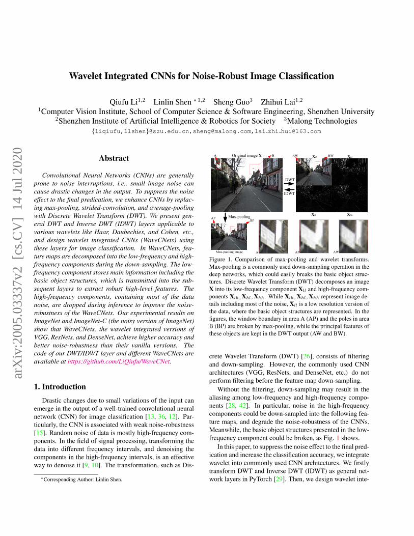
Figure 1. Comparison of max-pooling and wavelet transforms.Max-pooling is a commonly used down-sampling operation in thedeep networks, which could easily breaks the basic object struc-tures. Discrete Wavelet Transform (DWT) decomposes an imageX into its low-frequency component Xll and high-frequency com-ponents Xlh,Xhl,Xhh. While Xlh,Xhl,Xhh represent image de-tails including most of the noise, Xll is a low resolution version ofthe data, where the basic object structures are represented. In thefigures, the window boundary in area A (AP) and the poles in areaB (BP) are broken by max-pooling, while the principal features ofthese objects are kept in the DWT output (AW and BW).
crete Wavelet Transform (DWT) [26], consists of filteringand down-sampling. However, the commonly used CNNarchitectures (VGG, ResNets, and DenseNet, etc.) do notperform filtering before the feature map down-sampling.
Without the filtering, down-sampling may result in thealiasing among low-frequency and high-frequency compo-nents [28, 42]. In particular, noise in the high-frequencycomponents could be down-sampled into the following fea-ture maps, and degrade the noise-robustness of the CNNs.Meanwhile, the basic object structures presented in the low-frequency component could be broken, as Fig. 1 shows.
In this paper, to suppress the noise effect to the final pred-ication and increase the classification accuracy, we integratewavelet into commonly used CNN architectures. We firstlytransform DWT and Inverse DWT (IDWT) as general net-work layers in PyTorch [29]. Then, we design wavelet inte-
arX
iv:2
005.
0333
7v2
[cs
.CV
] 1
4 Ju
l 202
0
grated convolutional network (WaveCNet), by replacing thecommonly used down-sampling with DWT. During down-sampling, WaveCNet eliminates the high-frequency compo-nents of the feature maps to increase the noise-robustnessof the CNNs, and then extracts high-level features fromthe low-frequency component for better classification accu-racy. Using ImageNet [8] and ImageNet-C [15], we eval-uate WaveCNets in terms of classification accuracy andnoise-robustness, when various wavelets and various CNNarchitectures are used. At last, we explore the applicationof DWT/IDWT layer in image segmentation. In summary:
1. We present general DWT/IDWT layer applicable tovarious wavelets, which could be used to design end-to-end wavelet integrated deep networks.
2. We design WaveCNets by replacing existing down-sampling operations with DWT to improve the clas-sification accuracy and noise-robustness of CNNs.
3. We evaluate WaveCNets on ImageNet, and achieve in-creased accuracy and better noise-robustness.
4. The proposed DWT/IDWT layer is further integratedinto SegNet [2] to improve the segmentation perfor-mance of encoder-decoder networks.
2. Related works2.1. Noise-robustness
When the input image is changed, the output of CNN canbe significantly different, regardless of whether the changecan be easily perceived by human or not [13, 12, 21, 36].While the changes may result from various factors, such asshift [42, 25], rotation [5], noise [36], blur [15], manual at-tack [13], etc., we focus on the robustness of CNNs to thecommon noise. A high-level representation guided denoiseris designed in [21] to denoise the contaminated image be-fore inputting it into the CNN, which may complicate thewhole deep network structure. In [36], the authors proposedenoising block for CNNs to denoise the feature map andsuppress the effect of noise on the final prediction. How-ever, the authors design their denoising block using the spa-cial filtering, such as Gaussian filtering, mean filtering, andmedian filtering, etc., which do denoising in the whole fre-quency domain and may break basic object structure con-tained in the low-frequency component. Therefore, theirdenoising block requires a residual structure for the CNN toconverge. Recently, a benchmark evaluating CNN perfor-mance on noisy images is proposed in [15]. Our WaveC-Nets will be evaluated using this benchmark.
The recent studies show that ImageNet-trained CNNsprefer to extract features from object textures sensitive tonoise [3, 12]. Stylized ImageNet [12] is proposed via styliz-ing ImageNet images with style transfer to enable the CNNsto extract more robust features from object structures. The
noise could be enlarged as the feature maps flow throughlayers in the CNNs [21, 36], resulting in the final wrong pre-dictions. These issues may be related to the down-samplingoperations ignoring the classic sampling theorem.
2.2. Down-sampling
For local connectivity and weight sharing, researchersintroduce into deep networks various down-sampling op-erations, such as max-pooling, average-pooling, mixed-pooling, stochastic pooling, and strided-convolution, etc.While max-pooling and average-pooling are simple and ef-fective, they can erase or dilute details from images [38,40]. Although mixed-pooling [38] and stochastic pooling[40] are introduced to address these issues, max-pooling,average-pooling, and strided-convolution are still the mostwidely used operations in CNNs [14, 16, 31, 33].
These down-sampling operations usually ignore the clas-sic sampling theorem [1, 42], which could break objectstructures and accumulate noise. Fig. 1 shows a max-pooling example. Anti-aliased CNNs [42] integrate theclassic anti-aliasing filtering with the down-sampling. Theauthor is surprised at the increased classification accuracyand better noise-robustness. Compared to the anti-aliasedCNNs, our WaveCNets are significantly different in twoaspects: (1) While Max operation is still used in anti-aliased CNNs, WaveCNets do not require such operation.(2) The low-pass filters used in anti-aliased CNNs are em-pirically designed based on the row vectors of Pascal’s tri-angle, which is ad hoc and no theoretical justifications aregiven. As no up-sampling operation, i.e., reconstruction, ofthe low-pass filter is available, the anti-aliased U-Net [42]has to apply the same filtering after normal up-sampling toachieve the anti-aliasing effect. In comparison, our WaveC-Nets are justified by the well defined wavelet theory [6, 26].Both down-sampling and up-sampling can be replaced byDWT and IDWT, respectively.
In deep networks for image-to-image translation tasks,the up-sampling operations, such as transposed convolutionin U-Net [30] and max-unpooling in SegNet [2], are widelyapplied to upgrade the feature map resolution. Due to theabsence of the strict mathematical terms, these up-samplingoperations can not precisely recover the original data. Theydo not perform well in the restoration of image details.
2.3. Wavelets
Wavelets [6, 26] are powerful time-frequency analysistools, which have wide applications in signal processing.While Discrete Wavelet Transform (DWT) decompose adata into various components in different frequency inter-vals, Inverse DWT (IDWT) could reconstruct the data usingthe DWT output. DWT could be applied for anti-aliasingin signal processing, and we will explore its application indeep networks. IDWT could be used for detail restoration
in image-to-image tasks.
Wavelet has been combined with neural network forfunction approximation [41], signal representation and clas-sification [34]. In these early works, the authors applyshallow networks to search the optimal wavelet in waveletparameter domain. Recently, this method is utilized withdeeper network for image classification, but the network isdifficult to train because of the significant amount of com-putational cost [7]. ScatNet [5] cascades wavelet trans-form with nonlinear modulus and average pooling, to ex-tract a translation invariant feature robust to deformationsand preserve high-frequency information for image clas-sification. The authors introduce ScatNet when they ex-plore from mathematical and algorithmic perspective howto design the optimal deep network. Compared with theCNNs of the same period, ScatNet gets better performanceon the handwritten digit recognition and texture discrimina-tion tasks. However, due to the strict mathematical assump-tions, ScatNet can not be easily transferred to other tasks.
In deep learning, wavelets commonly play the roles ofimage preprocessing or postprocessing [17, 23, 32, 39].Meanwhile, researchers try to introduce wavelet trans-forms into the design of deep networks in various tasks[22, 35, 11, 37], by taking wavelet transforms as samplingoperations. Multi-level Wavelet CNN (MWCNN) proposedin [22] integrates Wavelet Package Transform (WPT) intothe deep network for image restoration. MWCNN concate-nates the low-frequency and high-frequency components ofthe input feature map, and processes them in a unified way,while the data distribution in these components significantlydiffers from each other. Convolutional-Wavelet Neural Net-work (CWNN) proposed in [11] applies dual-tree complexwavelet transform (DT-CWT) to suppress the noise andkeep the structures for extracting robust features from SARimages. The architecture of CWNN contains only two con-volution layers. While DT-CWT is redundant, CWNN takesas its down-sampling output the average value of the mul-tiple components output from DT-CWT. Wavelet poolingproposed in [35] is designed using a two-level DWT. Itsback-propagation performs a one-level DWT and a two-level IDWT, which does not follow the mathematical prin-ciple of gradient. The authors test their method on vari-ous dataset (MNIST [20], CIFAR-10 [18], SHVN [27], andKDEF [24]). However, their network architectures containonly four or five convolutional layers. The authors do notstudy systematically the potential of the method on standardimage dataset like ImageNet [8]. Recently, the applicationof wavelet transform in image style transfer is studied in[37]. In above works, the authors evaluate their methodswith only one or two wavelets, due to the absence of thegeneral wavelet transform layers.
3. Our methodOur method is trying to apply wavelet transforms to im-
prove the down-sampling operations in deep networks. Wefirstly design the general DWT and IDWT layers.
3.1. DWT and IDWT layers
The key issues in designs of DWT and IDWT layers arethe data forward and backward propagations. Although thefollowing analysis is for orthogonal wavelet and 1D signal,it can be generalized to other wavelets and 2D/3D signalwith only slight changes.
Forward propagation For a 1D signal s = {sj}j∈Z,DWT decomposes it into its low-frequency component s1 ={s1k}k∈Z and high-frequency component d1 = {d1k}k∈Z,where {
s1k =∑
j lj−2ksj ,
d1k =∑
j hj−2ksj ,(1)
and l = {lk}k∈Z,h = {hk}k∈Z are the low-pass and high-pass filters of an orthogonal wavelet. According to Eq. (1),DWT consists of filtering and down-sampling.
Using IDWT, one can reconstruct s from s1,d1, where
sj =∑k
(lj−2ks1k + hj−2kd1k) . (2)
In expressions with matrices and vectors, Eq. (1) and Eq.(2) can be rewritten as
s1 = Ls, d1 = Hs, (3)
s = LT s1 + HT d1, (4)
where
L =
· · · · · · · · ·· · · l−1 l0 l1 · · ·
· · · l−1 l0 l1 · · ·· · · · · ·
, (5)
H =
· · · · · · · · ·· · · h−1 h0 h1 · · ·
· · · h−1 h0 h1 · · ·· · · · · ·
. (6)
For 2D signal X, the DWT usually do 1D DWT on itsevery row and column, i.e.,
Xll = LXLT , (7)
Xlh = HXLT , (8)
Xhl = LXHT , (9)
Xhh = HXHT , (10)
and the corresponding IDWT is implemented with
X = LT XllL + HT XlhL + LT XhlH + HT XhhH. (11)
MaxPool(stride 2)
DWTll
AvgPool(stride 2)
DWTll
Conv(stride 2)
DWTllConv(stride 1)
(a)
(b)
Max Pooling Strided Convolution Average Pooling
Noisy Data X
DWT
Xll
Xlh, Xhl, Xhh
Denoising operations
Xlh, Xhl, Xhh
IDWT Denoised Data X
Noisy Data X
DWTll Xll
Noisy Data X
DWT
Denoising operations
Noisy Data X
DWTll Xll
Xlh, Xhl, Xhh
Xlh, Xhl, Xhh
Xll
Denoised Data X
IDWT
Noisy Data X
DWT
Xll
Xlh
Xhl
Xhh
Denoising operations Xlh
Xhl
Xhh
IDWT Denoised Data X
Data XDWTll Xll
Data X [Xll, Xlh, Xhl, Xhh]
Data X (Xll + Xlh + Xhl + Xhh)/4Average DWT
Concatenate DWT
(a) The general denoising approach using wavelet.
MaxPool(stride 2)
DWTll
AvgPool(stride 2)
DWTll
Conv(stride 2)
DWTllConv(stride 1)
(a)
(b)
Max Pooling Strided Convolution Average Pooling
Noisy Data X
DWT
Xll
Xlh, Xhl, Xhh
Denoising operations
Xlh, Xhl, Xhh
IDWT Denoised Data X
Noisy Data X
DWTll Xll
Noisy Data X
DWT
Denoising operations
Noisy Data X
DWTll Xll
Xlh, Xhl, Xhh
Xlh, Xhl, Xhh
Xll
Denoised Data X
IDWT
Noisy Data X
DWT
Xll
Xlh
Xhl
Xhh
Denoising operations Xlh
Xhl
Xhh
IDWT Denoised Data X
Data XDWTll Xll
Data X [Xll, Xlh, Xhl, Xhh]
Data X (Xll + Xlh + Xhl + Xhh)/4Average DWT
Concatenate DWT
(b) The simplest wavelet based “denoising” method, DWTll.
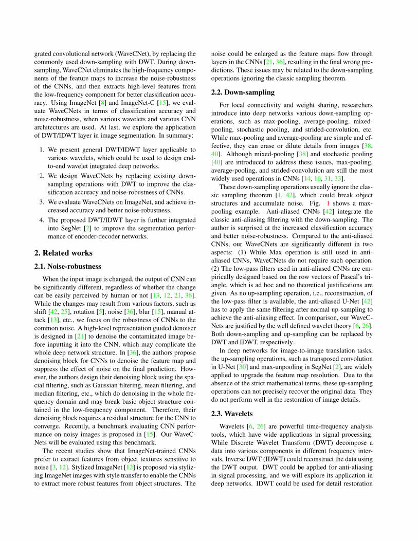
Figure 2. The general denoising approach based on wavelet trans-forms and the one used in WaveCNet.
Backward propagation For the backward propaga-tion of DWT, we start from Eq. (3) and differentiate it,
∂s1∂s
= LT ,∂d1
∂s= HT . (12)
Similarly, for the back propagation of the 1D IDWT, differ-entiate Eq. (4),
∂s∂s1
= L,∂s∂d1
= H. (13)
The forward and backward propagations of 2D/3D DWTand IDWT are slightly more complicated, but similar tothat of 1D DWT and IDWT. In practice, we choose thewavelets with finite filters, for example, Haar wavelet withl = 1√
2{1, 1} and h = 1√
2{1,−1}. For finite signal s ∈ RN
and X ∈ RN×N , the L,H are truncated to be the size ofbN2 c × N . We transform 1D/2D/3D DWT and IDWT asnetwork layers in PyTorch. In the layers, we do DWT andIDWT channel by channel for multi-channel data.
3.2. WaveCNets
Given a noisy 2D data X, the random noise mostly showup in its high-frequency components. Therefore, as Fig.2(a) shows, the general wavelet based denoising [9, 10]consists of three steps: (1) decompose the noisy data Xusing DWT into low-frequency component Xll and high-frequency components Xlh,Xhl,Xhh, (2) filter the high-frequency components, (3) reconstruct the data with theprocessed components using IDWT.
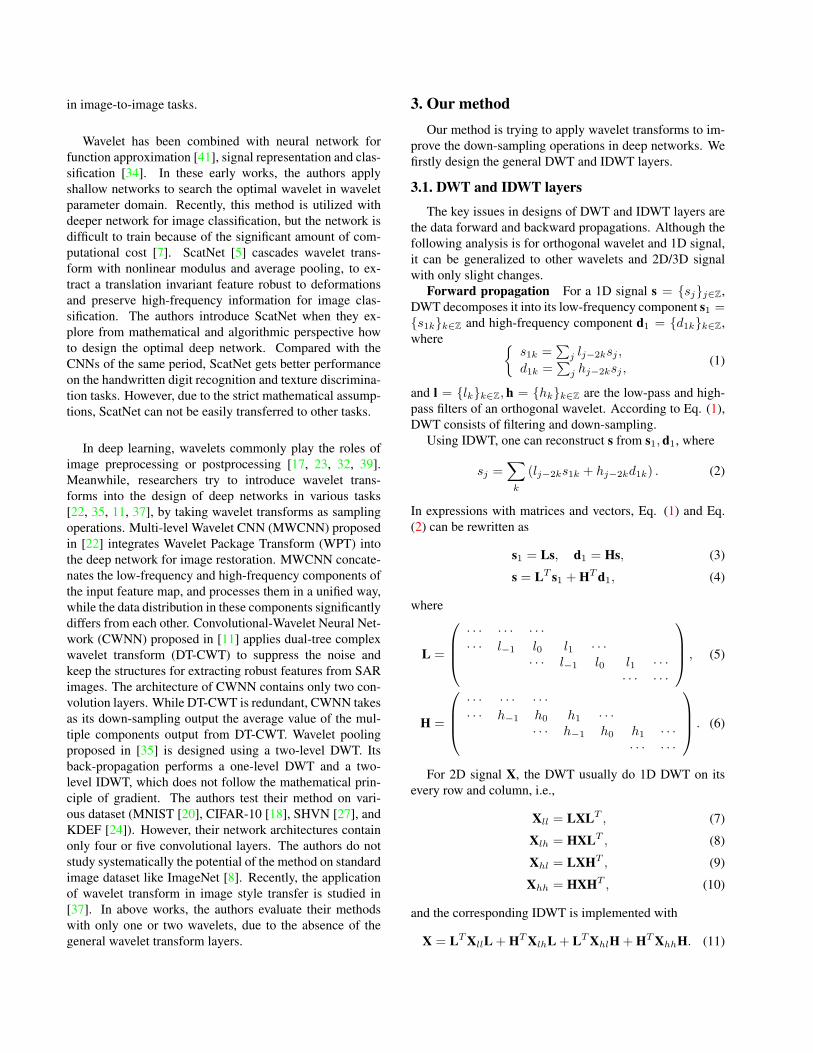
In this paper, we choose the simplest wavelet based “de-noising”, i.e., dropping the high-frequency components, asFig. 2(b) shows. DWTll denotes the transform mappingthe feature maps to the low-frequency component. We de-sign WaveCNets by replacing the commonly used down-sampling with DWTll. As Fig. 3 shows, in WaveCNets,max-pooling and average-pooling are directly replaced byDWTll, while strided-convolution is upgrated using convo-
MaxPool(stride 2)
DWTll
AvgPool(stride 2)
DWTll
Conv(stride 2)
DWTllConv(stride 1)
(a)
(b)
Max Pooling Strided Convolution Average Pooling
Noisy Data X
DWT
Xll
Xlh, Xhl, Xhh
Denoising operations
Xlh, Xhl, Xhh
IDWT Denoised Data X
Noisy Data X
DWTll Xll
Noisy Data X
DWT
Denoising operations
Noisy Data X
DWTll Xll
Xlh, Xhl, Xhh
Xlh, Xhl, Xhh
Xll
Denoised Data X
IDWT
Noisy Data X
DWT
Xll
Xlh
Xhl
Xhh
Denoising operations Xlh
Xhl
Xhh
IDWT Denoised Data X
Data XDWTll Xll
Data X [Xll, Xlh, Xhl, Xhh]
Data X (Xll + Xlh + Xhl + Xhh)/4Average DWT
Concatenate DWT
Figure 3. (a) Baseline, the down-sampling operations in deep net-works. (b) Wavelet integrated down-sampling in WaveCNets.
lution with stride of 1 followed by DWTll, i.e.,
MaxPools=2 → DWTll, (14)Convs=2 → DWTll ◦ Convs=1, (15)
AvgPools=2 → DWTll, (16)
where “MaxPools”, “Convs” and “AvgPools” denotethe max-pooling, strided-convolution, and average-poolingwith stride s, respectively.
While DWTll halves the size of the feature maps, it re-moves their high-frequency components and denoises them.The output of DWTll, i.e., the low-frequency component,saves the main information of the feature map to extractthe identifiable features. During down-sampling of WaveC-Nets, DWTll could resist the noise propagation in the deepnetworks and helps to maintain the basic object structurein the feature maps. Therefore, DWTll would acceler-ate the training of deep networks and lead to better noise-robustness and increased classification accuracy.
4. ExperimentsThe commonly used CNN architectures for image clas-
sification, such as VGG [33], ResNets [14], DenseNet[16], compose of various max-pooling, average-pooling,and strided-convolution. By upgrading the down-samplingwith Eqs. (14) - (16), we create WaveCNets, includ-ing WVGG16bn, WResNets, WDenseNet121. Comparedwith the original CNNs, WaveCNets do not employ addi-tional learnable parameters. We evaluate their classifica-tion accuracies and noise-robustness using ImageNet [8]and ImageNet-C [15]. At last, we explore the potential ofwavelet integrated deep networks for image segmentation.
4.1. ImageNet classification
ImageNet contains 1.2M training and 50K validationimages from 1000 categories. On the training set, wetrain WaveCNets when various wavelets are used, with thestandard training protocols from the publicly available Py-Torch [29] repository. Table 1 presents the top-1 accuracyof WaveCNets on ImageNet validation set, where “haar”,“dbx”, and “chx.y” denote the Haar wavelet, Daubechieswavelet with approximation order x, and Cohen waveletwith orders (x, y). The length of the wavelet filters increase
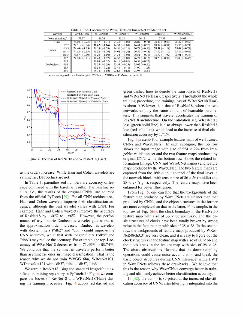
Table 1. Top-1 accuracy of WaveCNets on ImageNet validation set.Wavelet WVGG16bn WResNet18 WResNet34 WResNet50 WResNet101 WDenseNet121
None (baseline)* 73.37 69.76 73.30 76.15 77.37 74.65Haar 74.10 (+0.73) 71.47 (+1.71) 74.35 (+1.05) 76.89 (+0.74) 78.23 (+0.86) 75.27 (+0.62)
Cohen
ch2.2 74.31 (+0.94) 71.62 (+1.86) 74.33 (+1.03) 76.41 (+0.26) 78.34 (+0.97) 75.36 (+0.71)ch3.3 74.40 (+1.03) 71.55 (+1.79) 74.51 (+1.21) 76.71 (+0.56) 78.51 (+1.14) 75.44 (+0.79)ch4.4 74.02 (+0.65) 71.52 (+1.76) 74.61 (+1.31) 76.56 (+0.41) 78.47 (+1.10) 75.29 (+0.64)ch5.5 73.67 (+0.30) 71.26 (+1.50) 74.34 (+1.04) 76.51 (+0.36) 78.39 (+1.02) 75.01 (+0.36)
Daubechies
db2 74.08 (+0.71) 71.48 (+1.72) 74.30 (+1.00) 76.27 (+0.12) 78.29 (+0.92) 75.08 (+0.43)db3 71.08 (+1.32) 74.11 (+0.81) 76.38 (+0.23)db4 70.35 (+0.59) 73.53 (+0.23) 75.65 (−0.50)db5 69.54 (−0.22) 73.41 (+0.11) 74.90 (−1.25)db6 68.74 (−1.02) 72.68 (−0.62) 73.95 (−2.20)
* corresponding to the results of original CNNs, i.e., VGG16bn, ResNets, DenseNet121.
0 10 20 30 40 50 60 70 80epoch
1.2
1.4
1.6
1.8
2.0
2.2
2.4
2.6
loss
ResNet18 on Training DataResNet18 on Validation DataWResNet18(Haar) on Training DataWResNet18(Haar) on Validation Data
Figure 4. The loss of ResNet18 and WResNet18(Haar).
as the orders increase. While Haar and Cohen wavelets aresymmetric, Daubechies are not.
In Table 1, parenthesized numbers are accuracy differ-ence compared with the baseline results. The baseline re-sults, i.e., the results of the original CNNs, are sourcedfrom the official PyTorch [29]. For all CNN architectures,Haar and Cohen wavelets improve their classification ac-curacy, although the best wavelet varies with CNN. Forexample, Haar and Cohen wavelets improve the accuracyof ResNet18 by 1.50% to 1.86%. However, the perfor-mance of asymmetric Daubechies wavelet gets worse asthe approximation order increases. Daubechies waveletswith shorter filters (“db2” and “db3”) could improve theCNN accuracy, while that with longer filters (“db5” and“db6”) may reduce the accuracy. For example, the top-1 ac-curacy of WResNet18 decreases from 71.48% to 68.74%.We conclude that the symmetric wavelets perform betterthan asymmetric ones in image classification. That is thereason why we do not train WVGG16bn, WResNet101,WDenseNet121 with “db3”, “db4”, “db5”, “db6”.
We retrain ResNet18 using the standard ImageNet clas-sification training repository in PyTorch. In Fig. 4, we com-pare the losses of ResNet18 and WResNet18(Haar) dur-ing the training procedure. Fig. 4 adopts red dashed and
green dashed lines to denote the train losses of ResNet18and WResNet18(Haar), respectively. Throughout the wholetraining procedure, the training loss of WResNet18(Haar)is about 0.08 lower than that of ResNet18, when the twonetworks employ the same amount of learnable parame-ters. This suggests that wavelet accelerates the training ofResNet18 architecture. On the validation set, WResNet18loss (green solid line) is also always lower than ResNet18loss (red solid line), which lead to the increase of final clas-sification accuracy by 1.71%.
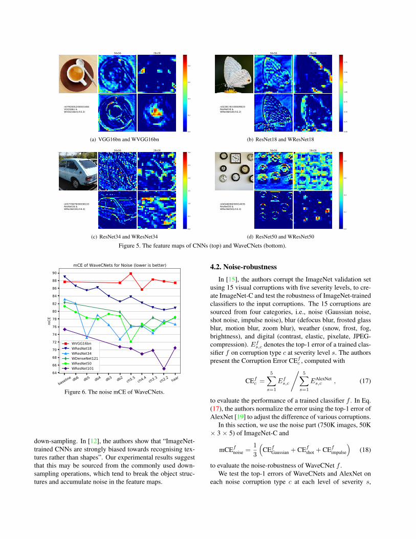
Fig. 5 presents four example feature maps of well trainedCNNs and WaveCNets. In each subfigure, the top rowshows the input image with size of 224 × 224 from Ima-geNet validation set and the two feature maps produced byoriginal CNN, while the bottom row shows the related in-formation (image, CNN and WaveCNet names) and featuremaps produced by the WaveCNet. The two feature maps arecaptured from the 16th output channel of the final layer inthe network blocks with tensor size of 56×56 (middle) and28 × 28 (right), respectively. The feature maps have beenenlarged for better illustration.
From Fig. 5, one can find that the backgrounds of thefeature map produced by WaveCNets are cleaner than thatproduced by CNNs, and the object structures in the formerare more complete than that in the latter. For example, in thetop row of Fig. 5(d), the clock boundary in the ResNet50feature map with size of 56 × 56 are fuzzy, and the ba-sic structures of clocks have been totally broken by strongnoise in the feature map with size of 28× 28. In the secondrow, the backgrounds of feature maps produced by WRes-Net50(ch3.3) are very clean, and it is easy to figure out theclock structures in the feature map with size of 56× 56 andthe clock areas in the feature map with size of 28 × 28.The above observations illustrate that the down-samplingoperations could cause noise accumulation and break thebasic object structures during CNN inference, while DWTin WaveCNets relieves these drawbacks. We believe thatthis is the reason why WaveCNets converge faster in train-ing and ultimately achieve better classification accuracy.
In [42], the author is surprised at the increased classifi-cation accuracy of CNNs after filtering is integrated into the
56x56 28x28
n07920052/00041584VGG16bn &WVGG16bn(ch3.3)
0.0
0.2
0.4
0.6
0.8
(a) VGG16bn and WVGG16bn
56x56 28x28
n02281787/00009023ResNet18 &WResNet18(ch2.2)
0.00
0.25
0.50
0.75
1.00
1.25
1.50
1.75
(b) ResNet18 and WResNet18
56x56 28x28
n03770679/00038133ResNet34 &WResNet34(ch4.4)
0.0
0.5
1.0
1.5
2.0
2.5
3.0
(c) ResNet34 and WResNet34
56x56 28x28
n04548280/00014035ResNet50 &WResNet50(ch3.3)
0.0
0.2
0.4
0.6
0.8
(d) ResNet50 and WResNet50
Figure 5. The feature maps of CNNs (top) and WaveCNets (bottom).
baseline db6 db5 db4 db3 db2ch5.5
ch4.4ch3.3
ch2.2 haar
Wavelet
64
66
68
70
72
74
76
78
80
82
84
86
88
90
mCE
mCE of WaveCNets for Noise (lower is better)
WVGG16bnWResNet18WResNet34WDenseNet121WResNet50WResNet101
Figure 6. The noise mCE of WaveCNets.
down-sampling. In [12], the authors show that “ImageNet-trained CNNs are strongly biased towards recognising tex-tures rather than shapes”. Our experimental results suggestthat this may be sourced from the commonly used down-sampling operations, which tend to break the object struc-tures and accumulate noise in the feature maps.
4.2. Noise-robustness
In [15], the authors corrupt the ImageNet validation setusing 15 visual corruptions with five severity levels, to cre-ate ImageNet-C and test the robustness of ImageNet-trainedclassifiers to the input corruptions. The 15 corruptions aresourced from four categories, i.e., noise (Gaussian noise,shot noise, impulse noise), blur (defocus blur, frosted glassblur, motion blur, zoom blur), weather (snow, frost, fog,brightness), and digital (contrast, elastic, pixelate, JPEG-compression). Ef
s,c denotes the top-1 error of a trained clas-sifier f on corruption type c at severity level s. The authorspresent the Corruption Error CEf
c , computed with
CEfc =
5∑s=1
Efs,c
/5∑
s=1
EAlexNets,c , (17)
to evaluate the performance of a trained classifier f . In Eq.(17), the authors normalize the error using the top-1 error ofAlexNet [19] to adjust the difference of various corruptions.
In this section, we use the noise part (750K images, 50K× 3 × 5) of ImageNet-C and
mCEfnoise =
1
3
(CEf
Gaussian + CEfshot + CEf
impulse
)(18)
to evaluate the noise-robustness of WaveCNet f .We test the top-1 errors of WaveCNets and AlexNet on
each noise corruption type c at each level of severity s,
input data ResNet18 WResNet18
0.0
0.2
0.4
0.6
0.8
1.0
1.2
1.4
(a) Gaussian noise
input data ResNet18 WResNet18
0.00
0.25
0.50
0.75
1.00
1.25
1.50
1.75
2.00
(b) Impulse noise
Figure 7. The feature maps sourced from clean (top) and noisy (bottom) images.
when WaveCNets and AlexNet are trained on the clean Im-ageNet training set. Then, we compute mCEWaveCNet
noise ac-cording to Eqs. (17) and (18). In Fig. 6, we show thenoise mCEs of WaveCNets for different network architec-tures and various wavelets. The “baseline” corresponds tothe noise mCEs of original CNN architectures, while “dbx”,“chx.y” and “haar” correspond to the mCEs of WaveCNetswith different wavelets. Except VGG16bn, our method ob-viously increase the noise-robustness of the CNN archi-tectures for image classification. For example, the noisemCE of ResNet18 (with navy blue color and down trian-gle marker in Fig. 6) decreases from 88.97 (“baseline”)to 80.38 (“ch2.2”). One can find that the all wavelets in-cluding “db5” and “db6” improve the noise-robustness ofResNet18, ResNet34, and ResNet50, although the classi-fication accuracy of the WResNets with “db5” and “db6”for the clean images may be lower than that of the origi-nal ResNets. It means that our methods indeed increase thenoise-robustness of these network architectures.
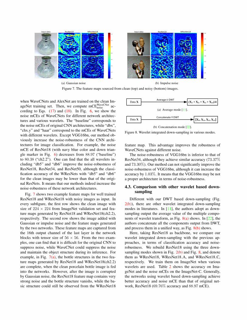
Fig. 7 shows two example feature maps for well trainedResNet18 and WResNet18 with noisy images as input. Inevery subfigure, the first row shows the clean image withsize of 224 × 224 from ImageNet validation set and fea-ture maps generated by ResNet18 and WResNet18(ch2.2),respectively. The second row shows the image added withGaussian or impulse noise and the feature maps generatedby the two networks. These feature maps are captured fromthe 16th output channel of the last layer in the networkblocks with tensor size of 56 × 56. From the two exam-ples, one can find that it is difficult for the original CNN tosuppress noise, while WaveCNet could suppress the noiseand maintain the object structure during its inference. Forexample, in Fig. 7(a), the bottle structures in the two fea-ture maps generated by ResNet18 and WResNet18(ch2.2)are complete, when the clean porcelain bottle image is fedinto the networks. However, after the image is corruptedby Gaussian noise, the ResNet18 feature map contains verystrong noise and the bottle structure vanishs, while the ba-sic structure could still be observed from the WResNet18
MaxPool(stride 2)
DWTll
AvgPool(stride 2)
DWTll
Conv(stride 2)
DWTllConv(stride 1)
(a)
(b)
Max Pooling Strided Convolution Average Pooling
Noisy Data X
DWT
Xll
Xlh, Xhl, Xhh
Denoising operations
Xlh, Xhl, Xhh
IDWT Denoised Data X
Noisy Data X
DWTll Xll
Noisy Data X
DWT
Denoising operations
Noisy Data X
DWTll Xll
Xlh, Xhl, Xhh
Xlh, Xhl, Xhh
Xll
Denoised Data X
IDWT
Noisy Data X
DWT
Xll
Xlh
Xhl
Xhh
Denoising operations Xlh
Xhl
Xhh
IDWT Denoised Data X
Data XDWTll Xll
Data X [Xll, Xlh, Xhl, Xhh]
Data X (Xll + Xlh + Xhl + Xhh)/4Average DWT
Concatenate DWT
(a) Average mode [11].
MaxPool(stride 2)
DWTll
AvgPool(stride 2)
DWTll
Conv(stride 2)
DWTllConv(stride 1)
(a)
(b)
Max Pooling Strided Convolution Average Pooling
Noisy Data X
DWT
Xll
Xlh, Xhl, Xhh
Denoising operations
Xlh, Xhl, Xhh
IDWT Denoised Data X
Noisy Data X
DWTll Xll
Noisy Data X
DWT
Denoising operations
Noisy Data X
DWTll Xll
Xlh, Xhl, Xhh
Xlh, Xhl, Xhh
Xll
Denoised Data X
IDWT
Noisy Data X
DWT
Xll
Xlh
Xhl
Xhh
Denoising operations Xlh
Xhl
Xhh
IDWT Denoised Data X
Data XDWTll Xll
Data X [Xll, Xlh, Xhl, Xhh]
Data X (Xll + Xlh + Xhl + Xhh)/4Average DWT
Concatenate DWT
(b) Concatenation mode [22].
Figure 8. Wavelet integrated down-sampling in various modes.
feature map. This advantage improves the robustness ofWaveCNets against different noise.
The noise-robustness of VGG16bn is inferior to that ofResNet34, although they achieve similar accuracy (73.37%and 73.30%). Our method can not significantly improve thenoise-robustness of VGG16bn, although it can increase theaccuracy by 1.03%. It means that the VGG16bn may be nota proper architecture in terms of noise-robustness.
4.3. Comparison with other wavelet based down-sampling
Different with our DWT based down-sampling (Fig.2(b)), there are other wavelet integrated down-samplingmodes in literatures. In [11], the authors adopt as down-sampling output the average value of the multiple compo-nents of wavelet transform, as Fig. 8(a) shows. In [22], theauthors concatenate all the components output from DWT,and process them in a unified way, as Fig. 8(b) shows.
Here, taking ResNet18 as backbone, we compare ourwavelet integrated down-sampling with the previous ap-proaches, in terms of classification accuracy and noise-robustness. We rebuild ResNet18 using the three down-sampling modes shown in Fig. 2(b) and Fig. 8, and denotethem as WResNet18, WResNet18 A, and WResNet18 C,respectively. We train them on ImageNet when variouswavelets are used. Table 2 shows the accuracy on Ima-geNet and the noise mCEs on the ImageNet-C. Generally,the networks using wavelet based down-sampling achievebetter accuracy and noise mCE than that of original net-work, ResNet18 (69.76% accuracy and 88.97 mCE).
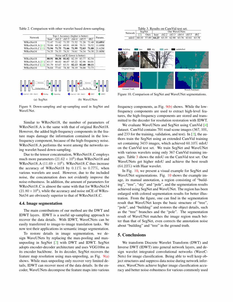
Table 2. Comparison with other wavelet based down-sampling.
Network Top-1 Accuracy (higher is better) Params.haar ch2.2 ch3.3 ch4.4 ch5.5 db2WResNet18 71.47 71.62 71.55 71.52 71.26 71.48 11.69MWResNet18 A [11] 70.06 69.24 69.91 69.98 70.31 70.52 11.69MWResNet18 C [22] 71.94 71.75 71.66 71.99 72.03 71.88 21.62MWResNet34 74.35 74.33 74.51 74.61 74.34 74.30 21.80M
Noise mCE (lower is better)WResNet18 80.91 80.38 81.02 82.19 83.77 82.54WResNet18 A [11] 83.17 86.02 86.07 85.22 82.96 84.01WResNet18 C [22] 81.79 83.67 83.51 82.13 82.60 80.11WResNet34 76.64 77.61 74.30 76.19 76.00 72.73
Tensor (Copy and Concatenate)
Mainstream
DeConvPoolingConv3x3 + BN + ReLU
Tensor (Copy and Plus)
Mainstream
DeConvPoolingConv3x3 + BN + ReLU
UnpoolingPoolingConv3x3 + BN + ReLU
Mainstream
Pooling Indices
IDWTDWTConv3x3 + BN + ReLU
Mainstream
Xlh, Xhl, Xhh
Xll
Mainstream
Xll, Xlh, Xhl, Xhh
Conv3x3 + BN + ReLU IDWTDWTPooling
(a) SegNet
Tensor (Copy and Concatenate)
Mainstream
DeConvPoolingConv3x3 + BN + ReLU
Tensor (Copy and Plus)
Mainstream
DeConvPoolingConv3x3 + BN + ReLU
UnpoolingPoolingConv3x3 + BN + ReLU
Mainstream
Pooling Indices
IDWTDWTConv3x3 + BN + ReLU
Mainstream
Xlh, Xhl, Xhh
Xll
Mainstream
Xll, Xlh, Xhl, Xhh
Conv3x3 + BN + ReLU IDWTDWTPooling
(b) WaveUNets
Figure 9. Down-sampling and up-sampling used in SegNet andWaveUNet.
Similar to WResNet18, the number of parameters ofWResNet18 A is the same with that of original ResNet18.However, the added high-frequency components in the fea-ture maps damage the information contained in the low-frequency component, because of the high-frequency noise.WResNet18 A performs the worst among the networks us-ing wavelet based down-sampling.
Due to the tensor concatenation, WResNet18 C employsmuch more parameters (21.62× 10⁶) than WResNet18 andWResNet18 A (11.69× 10⁶). WResNet18 C thus increasethe accuracy of WResNet18 by 0.11% to 0.77%, whenvarious wavelets are used. However, due to the includednoise, the concatenation does not evidently improve thenoise-robustness. In addition, the amount of parameters forWResNet18 C is almost the same with that for WResNet34(21.80×10⁶), while the accuracy and noise mCE of WRes-Net34 are obviously superior to that of WResNet18 C.
4.4. Image segmentation
The main contributions of our method are the DWT andIDWT layers. IDWT is a useful up-sampling approach torecover the data details. With IDWT, WaveCNets can beeasily transferred to image-to-image translation tasks. Wenow test their applications in semantic image segmentation.
To restore details in image segmentation, we de-sign WaveUNets by replacing the max-pooling and max-unpooling in SegNet [2] with DWT and IDWT. SegNetadopts encoder-decoder architecture and uses VGG16bn asits encoder backbone. In its decoder, SegNet recovers thefeature map resolution using max-unpooling, as Fig. 9(a)shows. While max-unpooling only recover very limited de-tails, IDWT can recover most of the data details. In the en-coder, WaveUNets decompose the feature maps into various
Table 3. Results on CamVid test set.Network SegNet Our WaveUNets
[2] Ours haar ch2.2 ch3.3 ch4.4 ch5.5 db2mIoU 60.10 57.89 64.23 63.35 62.90 63.76 63.61 63.78
sky buildingpole roadsidewalk treesymbol fencecar pedestrianbicyclist unlabelled
Original Image
Ground Truth
db6db5ch4.4 ch5.5
Original Image
Ground Truth
skybuilding poletree unlabelled
skybuildingtree carunlabelled
Original Image
Ground Truth
WPUNet(haar)
U-Net SegNet
WPUNet(ch5.5) WAUNet(ch5.5)
Original Image
Ground Truth db6db5 ch4.4 ch5.5
building road sidewalk
SegNet
WaveUNet(haar)
Figure 10. Comparison of SegNet and WaveUNet segmentations.
frequency components, as Fig. 9(b) shows. While the low-frequency components are used to extract high-level fea-tures, the high-frequency components are stored and trans-mitted to the decoder for resolution restoration with IDWT.
We evaluate WaveUNets and SegNet using CamVid [4]dataset. CamVid contains 701 road scene images (367, 101,and 233 for the training, validation, and test). In [2], the au-thors train the SegNet using an extended CamVid trainingset containing 3433 images, which achieved 60.10% mIoUon the CamVid test set. We train SegNet and WaveUNetwith various wavelets using only 367 CamVid training im-ages. Table 3 shows the mIoU on the CamVid test set. OurWaveUNets get higher mIoU and achieve the best result(64.23%) with Haar wavelet.
In Fig. 10, we present a visual example for SegNet andWaveUNet segmentations. Fig. 10 shows the example im-age, its manual annotation, a region consisting of “build-ing”, “tree”, “sky” and “pole”, and the segmentation resultsachieved using SegNet and WaveUNet. The region has beenenlarged with colored segmentation results for better illus-tration. From the figure, one can find in the segmentationresult that WaveUNet keeps the basic structure of “tree”,“pole”, and “building” and restores the object details, suchas the “tree” branches and the “pole”. The segmentationresult of WaveUNet matches the image region much bet-ter than that of SegNet, even corrects the annotation noiseabout “building” and “tree” in the ground truth.
5. ConclusionsWe transform Discrete Wavelet Transform (DWT) and
Inverse DWT (IDWT) into general network layers, and de-sign wavelet integrated convolutional networks (WaveC-Nets) for image classification. Being able to well keep ob-ject structures and suppress data noise during network infer-ence, WaveCNets achieve higher image classification accu-racy and better noise-robustness for various commonly used
network architectures.
Acknowledgments
The work was supported by the Natural Science Foun-dation of China under grants no. 61672357, 91959108and U1713214, and the Science and Technology Project ofGuangdong Province under grant no. 2018A050501014.
References[1] Aharon Azulay and Yair Weiss. Why do deep convolutional
networks generalize so poorly to small image transforma-tions? arXiv preprint arXiv:1805.12177, 2018. 2
[2] Vijay Badrinarayanan, Alex Kendall, and Roberto Cipolla.Segnet: A deep convolutional encoder-decoder architec-ture for image segmentation. IEEE transactions on PAMI,39(12):2481–2495, 2017. 2, 8
[3] Wieland Brendel and Matthias Bethge. Approximating cnnswith bag-of-local-features models works surprisingly well onimagenet. arXiv preprint arXiv:1904.00760, 2019. 2
[4] Gabriel J Brostow, Julien Fauqueur, and Roberto Cipolla.Semantic object classes in video: A high-definition groundtruth database. Pattern Recognition Letters, 30(2):88–97,2009. 8
[5] Joan Bruna and Stephane Mallat. Invariant scattering convo-lution networks. IEEE transactions on PAMI, 35(8):1872–1886, 2013. 2, 3
[6] Ingrid Daubechies. Ten lectures on wavelets, volume 61.Siam, 1992. 2
[7] DDN De Silva, HWMK Vithanage, KSD Fernando, andITS Piyatilake. Multi-path learnable wavelet neural networkfor image classification. arXiv preprint arXiv:1908.09775,2019. 3
[8] Jia Deng, Wei Dong, Richard Socher, Li-Jia Li, Kai Li,and Li Fei-Fei. Imagenet: A large-scale hierarchical imagedatabase. In 2009 IEEE conference on computer vision andpattern recognition, pages 248–255. Ieee, 2009. 2, 3, 4
[9] David L Donoho. De-noising by soft-thresholding. IEEEtransactions on information theory, 41(3):613–627, 1995. 1,4
[10] David L Donoho and Jain M Johnstone. Ideal spatial adapta-tion by wavelet shrinkage. biometrika, 81(3):425–455, 1994.1, 4
[11] Yiping Duan, Fang Liu, Licheng Jiao, Peng Zhao, and LuZhang. Sar image segmentation based on convolutional-wavelet neural network and markov random field. PatternRecognition, 64:255–267, 2017. 3, 7, 8
[12] Robert Geirhos, Patricia Rubisch, Claudio Michaelis,Matthias Bethge, Felix A Wichmann, and Wieland Brendel.Imagenet-trained cnns are biased towards texture; increasingshape bias improves accuracy and robustness. arXiv preprintarXiv:1811.12231, 2018. 1, 2, 6
[13] Ian J Goodfellow, Jonathon Shlens, and Christian Szegedy.Explaining and harnessing adversarial examples. arXivpreprint arXiv:1412.6572, 2014. 1, 2
[14] Kaiming He, Xiangyu Zhang, Shaoqing Ren, and Jian Sun.Deep residual learning for image recognition. In Proceed-ings of the IEEE conference on computer vision and patternrecognition, pages 770–778, 2016. 2, 4
[15] Dan Hendrycks and Thomas Dietterich. Benchmarking neu-ral network robustness to common corruptions and perturba-tions. arXiv preprint arXiv:1903.12261, 2019. 1, 2, 4, 6,11
[16] Gao Huang, Zhuang Liu, Laurens Van Der Maaten, and Kil-ian Q Weinberger. Densely connected convolutional net-works. In Proceedings of the IEEE conference on computervision and pattern recognition, pages 4700–4708, 2017. 2, 4
[17] Huaibo Huang, Ran He, Zhenan Sun, and Tieniu Tan.Wavelet-srnet: A wavelet-based cnn for multi-scale face su-per resolution. In Proceedings of the IEEE InternationalConference on Computer Vision, pages 1689–1697, 2017. 3
[18] Alex Krizhevsky, Geoffrey Hinton, et al. Learning multiplelayers of features from tiny images. Technical report, Cite-seer, 2009. 3
[19] Alex Krizhevsky, Ilya Sutskever, and Geoffrey E Hinton.Imagenet classification with deep convolutional neural net-works. In Advances in neural information processing sys-tems, pages 1097–1105, 2012. 6
[20] Yann LeCun, Leon Bottou, Yoshua Bengio, Patrick Haffner,et al. Gradient-based learning applied to document recog-nition. Proceedings of the IEEE, 86(11):2278–2324, 1998.3
[21] Fangzhou Liao, Ming Liang, Yinpeng Dong, Tianyu Pang,Xiaolin Hu, and Jun Zhu. Defense against adversarial attacksusing high-level representation guided denoiser. In Proceed-ings of the IEEE Conference on Computer Vision and PatternRecognition, pages 1778–1787, 2018. 2
[22] Pengju Liu, Hongzhi Zhang, Kai Zhang, Liang Lin, andWangmeng Zuo. Multi-level wavelet-cnn for image restora-tion. In Proceedings of the IEEE Conference on ComputerVision and Pattern Recognition Workshops, pages 773–782,2018. 3, 7, 8
[23] Yunfan Liu, Qi Li, and Zhenan Sun. Attribute enhanced faceaging with wavelet-based generative adversarial networks.arXiv preprint arXiv:1809.06647, 2018. 3
[24] Daniel Lundqvist, Anders Flykt, and Arne Ohman. Thekarolinska directed emotional faces (kdef). CD ROM fromDepartment of Clinical Neuroscience, Psychology section,Karolinska Institutet, 91:630, 1998. 3
[25] Julien Mairal, Piotr Koniusz, Zaid Harchaoui, and CordeliaSchmid. Convolutional kernel networks. In Advances in neu-ral information processing systems, pages 2627–2635, 2014.2
[26] Stephane G Mallat. A theory for multiresolution signal de-composition: the wavelet representation. IEEE Transactionson Pattern Analysis & Machine Intelligence, (7):674–693,1989. 1, 2
[27] Yuval Netzer, Tao Wang, Adam Coates, Alessandro Bis-sacco, Bo Wu, and Andrew Y Ng. Reading digits in naturalimages with unsupervised feature learning. 2011. 3
[28] Harry Nyquist. Certain topics in telegraph transmission the-ory. Transactions of the American Institute of Electrical En-gineers, 47(2):617–644, 1928. 1
[29] Adam Paszke, Sam Gross, Soumith Chintala, GregoryChanan, Edward Yang, Zachary DeVito, Zeming Lin, Al-ban Desmaison, Luca Antiga, and Adam Lerer. Automaticdifferentiation in pytorch. 2017. 1, 4, 5
[30] Olaf Ronneberger, Philipp Fischer, and Thomas Brox. U-net: Convolutional networks for biomedical image segmen-tation. In International Conference on MICCAI, pages 234–241. Springer, 2015. 2
[31] Mark Sandler, Andrew Howard, Menglong Zhu, Andrey Zh-moginov, and Liang-Chieh Chen. Mobilenetv2: Invertedresiduals and linear bottlenecks. In Proceedings of the IEEEConference on Computer Vision and Pattern Recognition,pages 4510–4520, 2018. 2
[32] Behrouz Alizadeh Savareh, Hassan Emami, MohamadrezaHajiabadi, Seyed Majid Azimi, and Mahyar Ghafoori.Wavelet-enhanced convolutional neural network: a newidea in a deep learning paradigm. Biomedical Engineer-ing/Biomedizinische Technik, 64(2):195–205, 2019. 3
[33] Karen Simonyan and Andrew Zisserman. Very deep convo-lutional networks for large-scale image recognition. arXivpreprint arXiv:1409.1556, 2014. 2, 4, 11
[34] Harold H Szu, Brian A Telfer, and Shubha L Kadambe. Neu-ral network adaptive wavelets for signal representation andclassification. Optical Engineering, 31(9):1907–1917, 1992.3
[35] Travis Williams and Robert Li. Wavelet pooling for con-volutional neural networks. In International Conference onLearning Representations, 2018. 3
[36] Cihang Xie, Yuxin Wu, Laurens van der Maaten, Alan LYuille, and Kaiming He. Feature denoising for improvingadversarial robustness. In Proceedings of the IEEE Con-ference on Computer Vision and Pattern Recognition, pages501–509, 2019. 1, 2
[37] Jaejun Yoo, Youngjung Uh, Sanghyuk Chun, ByeongkyuKang, and Jung-Woo Ha. Photorealistic style transfer viawavelet transforms. arXiv preprint arXiv:1903.09760, 2019.3
[38] Dingjun Yu, Hanli Wang, Peiqiu Chen, and Zhihua Wei.Mixed pooling for convolutional neural networks. In Inter-national Conference on Rough Sets and Knowledge Technol-ogy, pages 364–375. Springer, 2014. 2
[39] Binhang Yuan, Chen Wang, Fei Jiang, Mingsheng Long,Philip S Yu, and Yuan Liu. Waveletfcnn: A deep time seriesclassification model for wind turbine blade icing detection.arXiv preprint arXiv:1902.05625, 2019. 3
[40] Matthew D Zeiler and Rob Fergus. Stochastic pooling forregularization of deep convolutional neural networks. arXivpreprint arXiv:1301.3557, 2013. 2
[41] Qinghua Zhang and Albert Benveniste. Wavelet networks.IEEE transactions on Neural Networks, 3(6):889–898, 1992.3
[42] Richard Zhang. Making convolutional networks shift-invariant again. arXiv preprint arXiv:1904.11486, 2019. 1,2, 5, 11
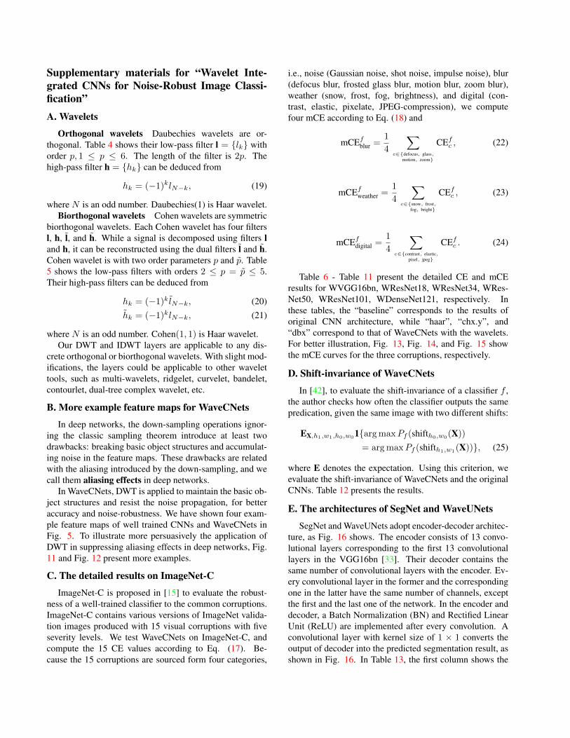
Supplementary materials for “Wavelet Inte-grated CNNs for Noise-Robust Image Classi-fication”A. Wavelets
Orthogonal wavelets Daubechies wavelets are or-thogonal. Table 4 shows their low-pass filter l = {lk} withorder p, 1 ≤ p ≤ 6. The length of the filter is 2p. Thehigh-pass filter h = {hk} can be deduced from
hk = (−1)klN−k, (19)
where N is an odd number. Daubechies(1) is Haar wavelet.Biorthogonal wavelets Cohen wavelets are symmetric
biorthogonal wavelets. Each Cohen wavelet has four filtersl, h, l, and h. While a signal is decomposed using filters land h, it can be reconstructed using the dual filters l and h.Cohen wavelet is with two order parameters p and p. Table5 shows the low-pass filters with orders 2 ≤ p = p ≤ 5.Their high-pass filters can be deduced from
hk = (−1)k lN−k, (20)hk = (−1)klN−k, (21)
where N is an odd number. Cohen(1, 1) is Haar wavelet.Our DWT and IDWT layers are applicable to any dis-
crete orthogonal or biorthogonal wavelets. With slight mod-ifications, the layers could be applicable to other wavelettools, such as multi-wavelets, ridgelet, curvelet, bandelet,contourlet, dual-tree complex wavelet, etc.
B. More example feature maps for WaveCNets
In deep networks, the down-sampling operations ignor-ing the classic sampling theorem introduce at least twodrawbacks: breaking basic object structures and accumulat-ing noise in the feature maps. These drawbacks are relatedwith the aliasing introduced by the down-sampling, and wecall them aliasing effects in deep networks.
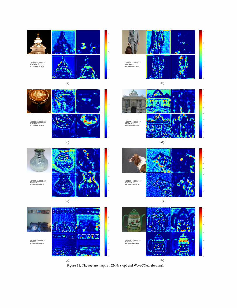
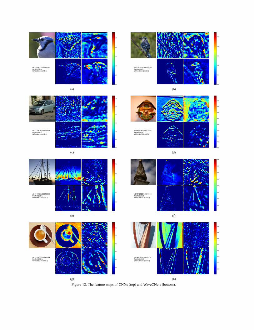
In WaveCNets, DWT is applied to maintain the basic ob-ject structures and resist the noise propagation, for betteraccuracy and noise-robustness. We have shown four exam-ple feature maps of well trained CNNs and WaveCNets inFig. 5. To illustrate more persuasively the application ofDWT in suppressing aliasing effects in deep networks, Fig.11 and Fig. 12 present more examples.
C. The detailed results on ImageNet-C
ImageNet-C is proposed in [15] to evaluate the robust-ness of a well-trained classifier to the common corruptions.ImageNet-C contains various versions of ImageNet valida-tion images produced with 15 visual corruptions with fiveseverity levels. We test WaveCNets on ImageNet-C, andcompute the 15 CE values according to Eq. (17). Be-cause the 15 corruptions are sourced form four categories,
i.e., noise (Gaussian noise, shot noise, impulse noise), blur(defocus blur, frosted glass blur, motion blur, zoom blur),weather (snow, frost, fog, brightness), and digital (con-trast, elastic, pixelate, JPEG-compression), we computefour mCE according to Eq. (18) and
mCEfblur =
1
4
∑c∈{defocus, glass,
motion, zoom}
CEfc , (22)
mCEfweather =
1
4
∑c∈{snow, frost,
fog, bright}
CEfc , (23)
mCEfdigital =
1
4
∑c∈{contrast, elastic,
pixel, jpeg}
CEfc . (24)
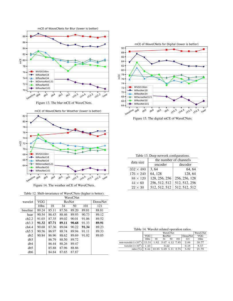
Table 6 - Table 11 present the detailed CE and mCEresults for WVGG16bn, WResNet18, WResNet34, WRes-Net50, WResNet101, WDenseNet121, respectively. Inthese tables, the “baseline” corresponds to the results oforiginal CNN architecture, while “haar”, “chx.y”, and“dbx” correspond to that of WaveCNets with the wavelets.For better illustration, Fig. 13, Fig. 14, and Fig. 15 showthe mCE curves for the three corruptions, respectively.
D. Shift-invariance of WaveCNets
In [42], to evaluate the shift-invariance of a classifier f ,the author checks how often the classifier outputs the samepredication, given the same image with two different shifts:
EX,h1,w1,h0,w01{argmaxPf (shifth0,w0
(X))
= argmaxPf (shifth1,w1(X))}, (25)
where E denotes the expectation. Using this criterion, weevaluate the shift-invariance of WaveCNets and the originalCNNs. Table 12 presents the results.
E. The architectures of SegNet and WaveUNets
SegNet and WaveUNets adopt encoder-decoder architec-ture, as Fig. 16 shows. The encoder consists of 13 convo-lutional layers corresponding to the first 13 convolutionallayers in the VGG16bn [33]. Their decoder contains thesame number of convolutional layers with the encoder. Ev-ery convolutional layer in the former and the correspondingone in the latter have the same number of channels, exceptthe first and the last one of the network. In the encoder anddecoder, a Batch Normalization (BN) and Rectified LinearUnit (ReLU) are implemented after every convolution. Aconvolutional layer with kernel size of 1 × 1 converts theoutput of decoder into the predicted segmentation result, asshown in Fig. 16. In Table 13, the first column shows the
Table 4. Low-pass filters of the Daubechies wavelets.p 1 2 3 4 5 6
lk
1 1 +√3 0.332670552950 0.230377813309 0.160102397974 0.111540743350
1 3 +√3 0.806891509311 0.714846570553 0.603829269797 0.494623890398
3−√3 0.459877502118 0.630880767930 0.724308528438 0.751133908021
1−√3 −0.135011020010 −0.027983769417 0.138428145901 0.315250351709−0.085441273882 −0.187034811719 −0.242294887066 −0.2262646939650.035226291886 0.030841381836 −0.032244869585 −0.129766867567
0.032883011667 0.077571493840 0.097501605587−0.010597401785 −0.006241490213 0.027522865530
−0.012580751999 −0.0315820393170.003335725285 0.000553842201
0.004777257511−0.001077301085
factor 1/√2 1/(4
√2) 1 1 1 1
Table 5. Low-pass filters of the Cohen wavelets.(p, p) (2, 2) (3, 3) (4, 4) (5, 5)
banks l l l l l l l l
lk
0 0 0 0.06629126 0 0 0.01345671 00.35355339 −0.17677670 0 −0.19887378 −0.06453888 0.03782846 −0.00269497 00.70710678 0.35355339 0.17677670 −0.15467961 −0.04068942 −0.02384947 −0.13670658 0.039687090.35355339 1.06066017 0.53033009 0.99436891 0.41809227 −0.11062440 −0.09350470 0.00794811
0 0.35355339 0.53033009 0.99436891 0.78848562 0.37740286 0.47680327 −0.054463790 −0.17677670 0.17677670 −0.15467961 0.41809227 0.85269868 0.89950611 0.34560528
0 −0.19887378 −0.04068942 0.37740286 0.47680327 0.736660180 0.06629126 −0.06453888 −0.11062440 −0.09350470 0.34560528
0 −0.02384947 −0.13670658 −0.054463790 0.03782846 −0.00269497 0.00794811
0.01345671 0.039687090 0
Table 6. Corruption Error (CE) of WVGG16bn on ImageNet-C (lower is better).Noise Blur Weather Digital
Gauss Shot Impulse mCE Defocus Glass Motion Zoom mCE Snow Frost Fog Bright mCE Contrast Elastic Pixel Jpeg mCEbaseline 86.28 87.48 89.11 87.62 83.95 94.80 86.36 87.56 88.17 83.25 79.98 72.06 63.53 74.70 75.02 95.22 94.87 88.88 88.50
haar 85.80 86.67 89.82 87.43 84.24 95.23 85.46 86.84 87.94 84.62 80.68 72.02 64.38 75.43 75.74 96.40 96.49 89.34 89.49ch2.2 87.29 87.80 88.29 87.79 83.63 95.63 84.91 86.08 87.56 82.70 80.65 71.55 63.64 74.63 74.66 96.17 92.95 90.34 88.53ch3.3 86.40 87.39 91.04 88.28 84.03 95.90 85.30 86.34 87.89 83.81 81.01 72.43 64.14 75.35 75.18 96.05 93.34 89.73 88.58ch4.4 85.01 85.45 86.44 85.63 84.34 95.58 85.77 86.59 88.07 84.21 82.11 73.02 64.73 76.02 76.62 96.72 91.19 90.13 88.67ch5.5 88.38 89.14 92.01 89.84 84.56 96.80 86.02 86.77 88.54 86.58 82.51 74.24 65.52 77.21 76.57 97.50 93.46 90.23 89.44
db2 86.54 88.27 87.51 87.44 84.46 95.69 85.43 86.41 88.00 84.37 81.46 72.94 64.76 75.88 76.57 96.35 93.14 90.86 89.23
Table 7. Corruption Error (CE) of WResNet18 on ImageNet-C (lower is better).Noise Blur Weather Digital
Gauss Shot Impulse mCE Defocus Glass Motion Zoom mCE Snow Frost Fog Bright mCE Contrast Elastic Pixel Jpeg mCEbaseline 87.15 88.47 91.30 88.97 83.82 91.43 86.82 88.70 87.69 86.10 84.40 78.48 68.90 79.47 78.29 90.23 80.40 85.46 83.60
haar 80.64 80.94 81.16 80.91 80.18 90.55 84.04 86.49 85.32 85.04 81.93 73.32 65.78 76.52 75.72 87.78 74.87 87.77 81.54ch2.2 80.15 80.49 80.50 80.38 79.65 89.79 83.61 84.82 84.47 84.91 80.84 73.99 66.34 76.52 75.07 88.19 75.07 88.61 81.73ch3.3 80.85 81.44 80.77 81.02 79.28 91.20 82.71 85.52 84.68 84.48 81.20 71.76 65.44 75.72 73.77 89.66 77.46 86.06 81.74ch4.4 81.83 82.65 82.10 82.19 79.55 91.01 82.88 84.55 84.50 83.91 80.81 73.95 66.27 76.23 75.67 90.21 78.35 86.10 82.58ch5.5 83.60 83.87 83.84 83.77 80.73 91.64 83.04 85.45 85.21 84.39 81.42 73.83 67.10 76.68 76.21 91.07 78.95 89.35 83.89
db2 82.30 82.65 82.68 82.54 80.16 91.22 83.55 84.73 84.92 85.42 81.74 74.34 66.51 77.00 75.92 90.41 79.54 91.71 84.39db3 83.75 84.14 83.87 83.92 81.36 90.92 84.14 86.24 85.66 85.01 81.73 75.79 68.14 77.67 78.47 90.02 78.41 89.35 84.06db4 86.00 85.83 86.85 86.22 82.12 92.93 85.75 87.38 87.04 85.31 83.02 77.87 68.97 78.79 79.33 91.07 74.95 85.63 82.74db5 85.22 85.86 85.33 85.47 82.96 92.65 87.83 88.63 88.02 87.60 85.21 78.66 71.33 80.70 80.85 91.11 78.21 92.99 85.79db6 86.29 86.73 86.68 86.57 84.72 94.50 87.73 88.68 88.91 87.88 86.62 80.58 72.81 81.97 82.29 93.46 78.32 95.53 87.40
input size, though these networks can process images witharbitrary size. Every number in the table corresponds to aconvolutional layer with BN and ReLU. While the numberin the column “encoder” is the number of the input channelsof the convolution, the number in the column “decoder” isthe number of the output channels.
F. The amount of multiply-adds in 2D DWT/IDWT
Given a 2D tensor X with size of M ×N and channel C,the amount of multiply-adds used in 2D DWT inference is
4C
(M2N +
MN2
2− 3MN
4
), (26)
n04346328/00011836VGG16bn &WVGG16bn(ch3.3)
0.0
0.2
0.4
0.6
0.8
1.0
(a)
n04350905/00003533VGG16bn &WVGG16bn(ch3.3)
0.0
0.1
0.2
0.3
0.4
0.5
0.6
0.7
0.8
(b)
n07920052/00028898VGG16bn &WVGG16bn(ch3.3)
0.0
0.1
0.2
0.3
0.4
0.5
0.6
0.7
0.8
(c)
n03877845/00024671ResNet18 &WResNet18(ch2.2)
0.0
0.2
0.4
0.6
0.8
1.0
1.2
1.4
1.6
(d)
n04522168/00031441ResNet18 &WResNet18(ch2.2)
0.0
0.2
0.4
0.6
0.8
1.0
1.2
1.4
(e)
n02102040/00010994ResNet18 &WResNet18(ch2.2)
0.0
0.2
0.4
0.6
0.8
1.0
1.2
1.4
1.6
(f)
n04033995/00009944ResNet34 &WResNet34(ch4.4)
0.0
0.5
1.0
1.5
2.0
2.5
3.0
3.5
(g)
n04398044/00019622ResNet34 &WResNet34(ch4.4)
0.0
0.5
1.0
1.5
2.0
2.5
3.0
(h)
Figure 11. The feature maps of CNNs (top) and WaveCNets (bottom).
n01580077/00032702ResNet34 &WResNet34(ch4.4)
0.0
0.5
1.0
1.5
2.0
2.5
(a)
n01580077/00026465ResNet34 &WResNet34(ch4.4)
0.0
0.5
1.0
1.5
2.0
2.5
(b)
n03770679/00007374ResNet34 &WResNet34(ch4.4)
0.0
0.5
1.0
1.5
2.0
2.5
3.0
(c)
n04548280/00018936ResNet50 &WResNet50(ch3.3)
0.0
0.1
0.2
0.3
0.4
0.5
0.6
0.7
0.8
(d)
n04147183/00026899ResNet101 &WResNet101(ch3.3)
0.1
0.2
0.3
0.4
0.5
(e)
n04346328/00024094ResNet101 &WResNet101(ch3.3)
0.05
0.10
0.15
0.20
0.25
0.30
0.35
0.40
(f)
n07920052/00041584ResNet101 &WResNet101(ch3.3)
0.05
0.10
0.15
0.20
0.25
0.30
(g)
n03495258/00039792ResNet101 &WResNet101(ch3.3)
0.05
0.10
0.15
0.20
0.25
0.30
0.35
0.40
(h)
Figure 12. The feature maps of CNNs (top) and WaveCNets (bottom).
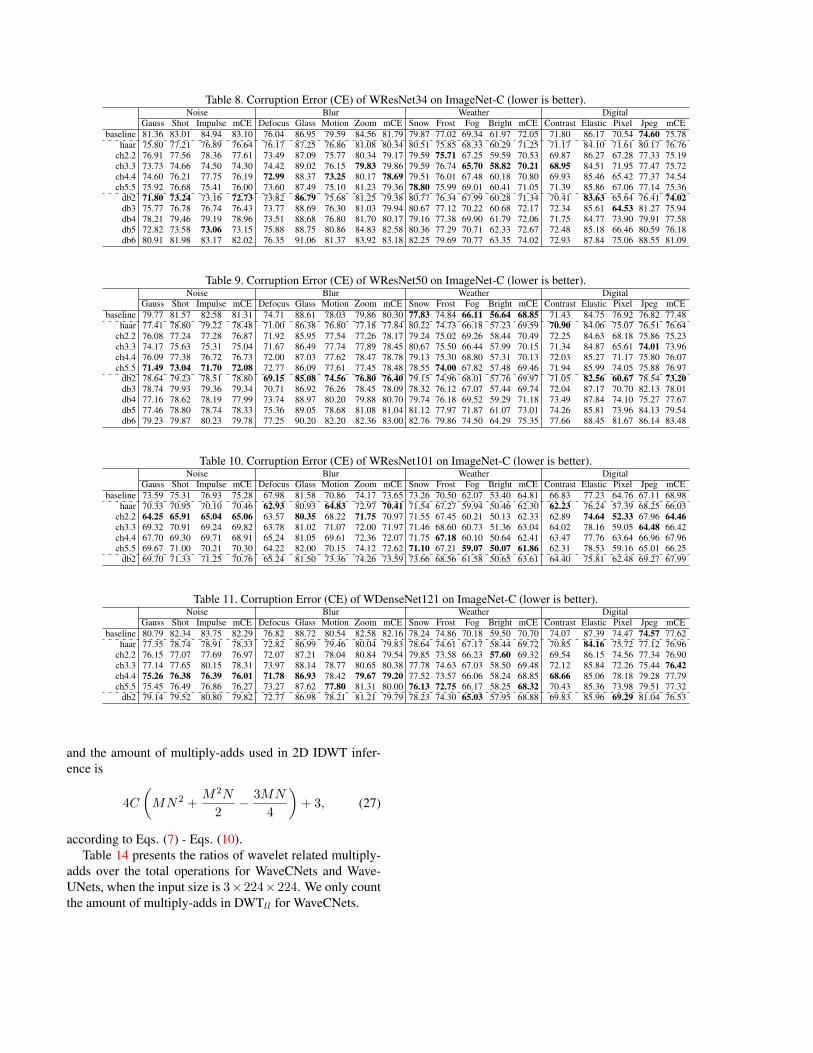
Table 8. Corruption Error (CE) of WResNet34 on ImageNet-C (lower is better).Noise Blur Weather Digital
Gauss Shot Impulse mCE Defocus Glass Motion Zoom mCE Snow Frost Fog Bright mCE Contrast Elastic Pixel Jpeg mCEbaseline 81.36 83.01 84.94 83.10 76.04 86.95 79.59 84.56 81.79 79.87 77.02 69.34 61.97 72.05 71.80 86.17 70.54 74.60 75.78
haar 75.80 77.21 76.89 76.64 76.17 87.25 76.86 81.08 80.34 80.51 75.85 68.33 60.29 71.25 71.17 84.10 71.61 80.17 76.76ch2.2 76.91 77.56 78.36 77.61 73.49 87.09 75.77 80.34 79.17 79.59 75.71 67.25 59.59 70.53 69.87 86.27 67.28 77.33 75.19ch3.3 73.73 74.66 74.50 74.30 74.42 89.02 76.15 79.83 79.86 79.59 76.74 65.70 58.82 70.21 68.95 84.51 71.95 77.47 75.72ch4.4 74.60 76.21 77.75 76.19 72.99 88.37 73.25 80.17 78.69 79.51 76.01 67.48 60.18 70.80 69.93 85.46 65.42 77.37 74.54ch5.5 75.92 76.68 75.41 76.00 73.60 87.49 75.10 81.23 79.36 78.80 75.99 69.01 60.41 71.05 71.39 85.86 67.06 77.14 75.36
db2 71.80 73.24 73.16 72.73 73.82 86.79 75.68 81.25 79.38 80.77 76.34 67.99 60.28 71.34 70.41 83.63 65.64 76.41 74.02db3 75.77 76.78 76.74 76.43 73.77 88.69 76.30 81.03 79.94 80.67 77.12 70.22 60.68 72.17 72.34 85.61 64.53 81.27 75.94db4 78.21 79.46 79.19 78.96 73.51 88.68 76.80 81.70 80.17 79.16 77.38 69.90 61.79 72.06 71.75 84.77 73.90 79.91 77.58db5 72.82 73.58 73.06 73.15 75.88 88.75 80.86 84.83 82.58 80.36 77.29 70.71 62.33 72.67 72.48 85.18 66.46 80.59 76.18db6 80.91 81.98 83.17 82.02 76.35 91.06 81.37 83.92 83.18 82.25 79.69 70.77 63.35 74.02 72.93 87.84 75.06 88.55 81.09
Table 9. Corruption Error (CE) of WResNet50 on ImageNet-C (lower is better).Noise Blur Weather Digital
Gauss Shot Impulse mCE Defocus Glass Motion Zoom mCE Snow Frost Fog Bright mCE Contrast Elastic Pixel Jpeg mCEbaseline 79.77 81.57 82.58 81.31 74.71 88.61 78.03 79.86 80.30 77.83 74.84 66.11 56.64 68.85 71.43 84.75 76.92 76.82 77.48
haar 77.41 78.80 79.22 78.48 71.00 86.38 76.80 77.18 77.84 80.22 74.73 66.18 57.23 69.59 70.90 84.06 75.07 76.51 76.64ch2.2 76.08 77.24 77.28 76.87 71.92 85.95 77.54 77.26 78.17 79.24 75.02 69.26 58.44 70.49 72.25 84.63 68.18 75.86 75.23ch3.3 74.17 75.63 75.31 75.04 71.67 86.49 77.74 77.89 78.45 80.67 75.50 66.44 57.99 70.15 71.34 84.87 65.61 74.01 73.96ch4.4 76.09 77.38 76.72 76.73 72.00 87.03 77.62 78.47 78.78 79.13 75.30 68.80 57.31 70.13 72.03 85.27 71.17 75.80 76.07ch5.5 71.49 73.04 71.70 72.08 72.77 86.09 77.61 77.45 78.48 78.55 74.00 67.82 57.48 69.46 71.94 85.99 74.05 75.88 76.97
db2 78.64 79.23 78.51 78.80 69.15 85.08 74.56 76.80 76.40 79.15 74.96 68.01 57.76 69.97 71.05 82.56 60.67 78.54 73.20db3 78.74 79.93 79.36 79.34 70.71 86.92 76.26 78.45 78.09 78.32 76.12 67.07 57.44 69.74 72.04 87.17 70.70 82.13 78.01db4 77.16 78.62 78.19 77.99 73.74 88.97 80.20 79.88 80.70 79.74 76.18 69.52 59.29 71.18 73.49 87.84 74.10 75.27 77.67db5 77.46 78.80 78.74 78.33 75.36 89.05 78.68 81.08 81.04 81.12 77.97 71.87 61.07 73.01 74.26 85.81 73.96 84.13 79.54db6 79.23 79.87 80.23 79.78 77.25 90.20 82.20 82.36 83.00 82.76 79.86 74.50 64.29 75.35 77.66 88.45 81.67 86.14 83.48
Table 10. Corruption Error (CE) of WResNet101 on ImageNet-C (lower is better).Noise Blur Weather Digital
Gauss Shot Impulse mCE Defocus Glass Motion Zoom mCE Snow Frost Fog Bright mCE Contrast Elastic Pixel Jpeg mCEbaseline 73.59 75.31 76.93 75.28 67.98 81.58 70.86 74.17 73.65 73.26 70.50 62.07 53.40 64.81 66.83 77.23 64.76 67.11 68.98
haar 70.33 70.95 70.10 70.46 62.93 80.93 64.83 72.97 70.41 71.54 67.27 59.94 50.46 62.30 62.23 76.24 57.39 68.25 66.03ch2.2 64.25 65.91 65.04 65.06 63.57 80.35 68.22 71.75 70.97 71.55 67.45 60.21 50.13 62.33 62.89 74.64 52.33 67.96 64.46ch3.3 69.32 70.91 69.24 69.82 63.78 81.02 71.07 72.00 71.97 71.46 68.60 60.73 51.36 63.04 64.02 78.16 59.05 64.48 66.42ch4.4 67.70 69.30 69.71 68.91 65.24 81.05 69.61 72.36 72.07 71.75 67.18 60.10 50.64 62.41 63.47 77.76 63.64 66.96 67.96ch5.5 69.67 71.00 70.21 70.30 64.22 82.00 70.15 74.12 72.62 71.10 67.21 59.07 50.07 61.86 62.31 78.53 59.16 65.01 66.25
db2 69.70 71.33 71.25 70.76 65.24 81.50 73.36 74.26 73.59 73.66 68.56 61.58 50.65 63.61 64.40 75.81 62.48 69.27 67.99
Table 11. Corruption Error (CE) of WDenseNet121 on ImageNet-C (lower is better).Noise Blur Weather Digital
Gauss Shot Impulse mCE Defocus Glass Motion Zoom mCE Snow Frost Fog Bright mCE Contrast Elastic Pixel Jpeg mCEbaseline 80.79 82.34 83.75 82.29 76.82 88.72 80.54 82.58 82.16 78.24 74.86 70.18 59.50 70.70 74.07 87.39 74.47 74.57 77.62
haar 77.35 78.74 78.91 78.33 72.82 86.99 79.46 80.04 79.83 78.64 74.61 67.17 58.44 69.72 70.85 84.16 75.72 77.12 76.96ch2.2 76.15 77.07 77.69 76.97 72.07 87.21 78.04 80.84 79.54 79.85 73.58 66.23 57.60 69.32 69.54 86.15 74.56 77.34 76.90ch3.3 77.14 77.65 80.15 78.31 73.97 88.14 78.77 80.65 80.38 77.78 74.63 67.03 58.50 69.48 72.12 85.84 72.26 75.44 76.42ch4.4 75.26 76.38 76.39 76.01 71.78 86.93 78.42 79.67 79.20 77.52 73.57 66.06 58.24 68.85 68.66 85.06 78.18 79.28 77.79ch5.5 75.45 76.49 76.86 76.27 73.27 87.62 77.80 81.31 80.00 76.13 72.75 66.17 58.25 68.32 70.43 85.36 73.98 79.51 77.32
db2 79.14 79.52 80.80 79.82 72.77 86.98 78.21 81.21 79.79 78.23 74.30 65.03 57.95 68.88 69.83 85.96 69.29 81.04 76.53
and the amount of multiply-adds used in 2D IDWT infer-ence is
4C
(MN2 +
M2N
2− 3MN
4
)+ 3, (27)
according to Eqs. (7) - Eqs. (10).Table 14 presents the ratios of wavelet related multiply-
adds over the total operations for WaveCNets and Wave-UNets, when the input size is 3×224×224. We only countthe amount of multiply-adds in DWTll for WaveCNets.
baseline db6 db5 db4 db3 db2ch5.5
ch4.4ch3.3
ch2.2 haar
Wavelet
70
72
74
76
78
80
82
84
86
88
mCE
mCE of WaveCNets for Blur (lower is better)
WVGG16bnWResNet18WResNet34WDenseNet121WResNet50WResNet101
Figure 13. The blur mCE of WaveCNets.
baseline db6 db5 db4 db3 db2ch5.5
ch4.4ch3.3
ch2.2 haar
Wavelet
64
66
68
70
72
74
76
78
80
82
mCE
mCE of WaveCNets for Weather (lower is better)
WVGG16bnWResNet18WResNet34WDenseNet121WResNet50WResNet101
Figure 14. The weather mCE of WaveCNets.
Table 12. Shift-invariance of WaveCNets (higher is better).
waveletWaveCNet
VGG ResNet DenseNet16bn 18 34 50 101 121
baseline 89.24 85.11 87.56 89.20 89.81 88.81haar 90.54 86.43 88.46 89.93 90.73 89.12
ch2.2 91.03 87.35 89.02 90.01 91.06 89.52ch3.3 91.32 87.71 89.11 90.68 91.33 89.91ch4.4 90.68 87.36 89.04 90.22 91.34 89.23ch5.5 90.56 86.97 88.74 89.94 91.11 89.33
db2 90.84 86.96 88.62 89.69 91.02 89.05db3 86.79 88.50 89.72db4 86.44 88.26 89.47db5 85.88 87.96 88.86db6 84.84 87.65 87.87
baseline db6 db5 db4 db3 db2ch5.5
ch4.4ch3.3
ch2.2 haar
Wavelet
6466687072747678808284868890
mCE
mCE of WaveCNets for Digital (lower is better)
WVGG16bnWResNet18WResNet34WDenseNet121WResNet50WResNet101
Figure 15. The digital mCE of WaveCNets.
Table 13. Deep network configurations.
data size the number of channelsencoder decoder
352× 480 3, 64 64, 64176× 240 64, 128 128, 6488× 120 128, 256, 256 256, 256, 12844× 60 256, 512, 512 512, 512, 25622× 30 512, 512, 512 512, 512, 512
Table 14. Wavelet related operation ratios.WaveCNet WaveUNet
VGG ResNet DenseNet VGG16bn 18 34 50 101 121 16bn
non-wavelet (×109) 15.51 1.82 3.67 4.12 7.85 2.88 30.77
wavelet (×109) 1.43 0.22 0.18 8.57ratio (%) 8.44 10.85 5.69 5.11 2.75 5.82 21.78
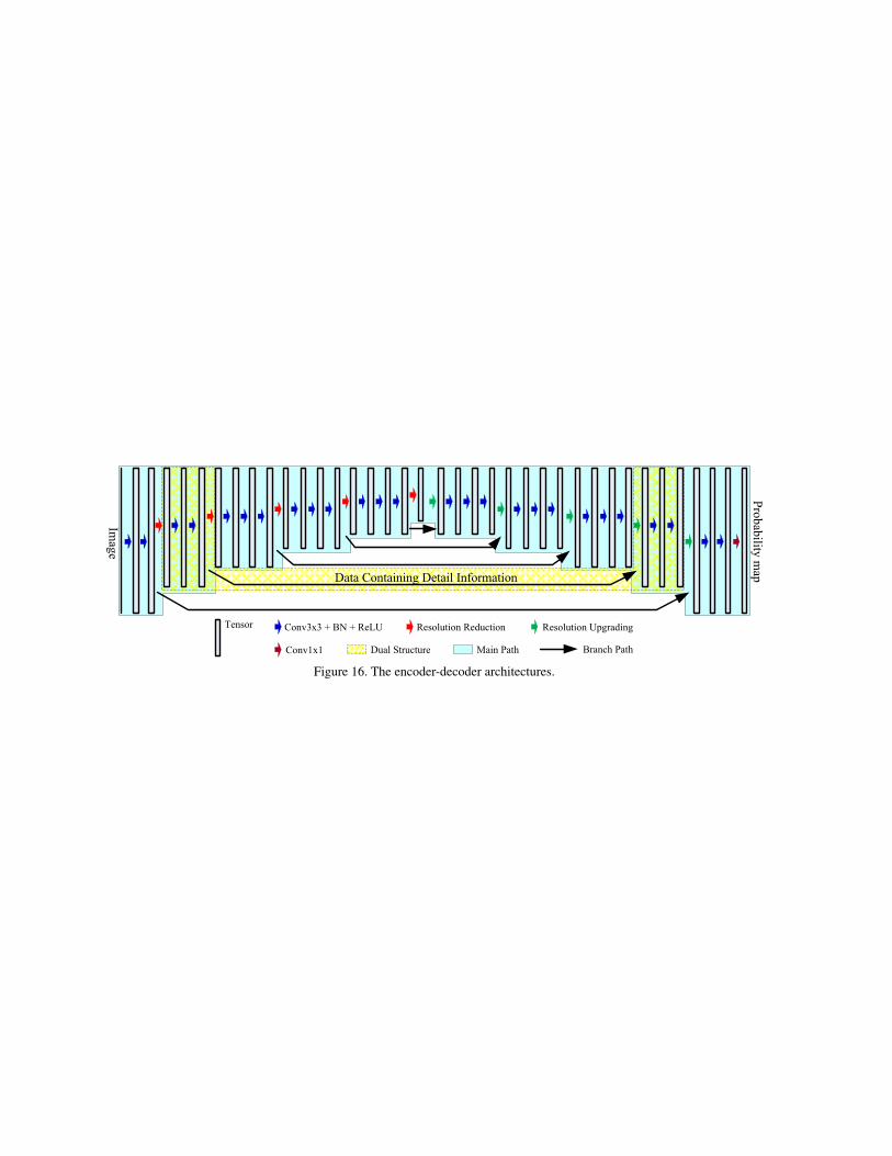
Image
Probability mapData Containing Detail Information
Image
Probability mapData Containing Detail Information
Dual Structure
Resolution Reduction Resolution Upgrading
Conv1x1Tensor
Branch Path
Conv3x3 + BN + ReLU
Dual Structure
Resolution Reduction Resolution Upgrading
Conv1x1
Tensor
Branch Path
Conv3x3 + BN + ReLU
Main Path
Figure 16. The encoder-decoder architectures.