Title of poster, about 15 words will fit on this line at 50 pt. Arial fontAuthors: First Name, Last Name, PhD1

Affiliations: 1 Group Health Research Institute, Name of other institute ResultsBackground

Choose systole and diastole training images manually. In practice, we find it difficult to initialize our weights. FC Layers are trained only after “good guess” by chance.

Try freezing VGG in different layers. Transferable learning should get better or worse with ConvNets.

Try different optimization methods and tune learning rate for our models.

Model

Diagnosis of Heart Disease via CNNs Yanyang Kong, Kaicheng Wang

Data & Preprocessing In the training dataset, we have 500 patients undergoing

averagely 10 experiments in different axis planes, like 2ch_16, 4ch_17, sax_5, sax_6, sax_7, sax_9, etc. Each experiment leads to 30 MRI across the cardiac cycle.

ProblemGiven a patient’s several (10 in average) MRI measurements in different axes (sax_5,…, 2ch_12, 4ch_32, etc), we are going to estimate end-distole volume and end-systole volume of left ventricle in one cardiac cycle. We aim to build two deep CNN models to predict two volumes using the same dataset.

Declining ejection fraction (EF) is a key indicator of heart disease.

Measuring cardiac end-systolic

and end-diastolic volumes (i.e., the size of one chamber of the heart at the beginning and middle of each heartbeat) and then derive the EF of heart is a standard process to assess the heart’s squeezing ability.

EF = 100 · VD � VS

VD

After partitioning the MRIs for each patient, we first preprocess the images by resizing or zero-padding to (224,224) dimensions and replicate the gray MRI image to 3 channels to fit VGG net. We also augment the data set by randomly rotate and shift slightly before putting to CNN.

We build two Axis-based CNN models for our problem, one to predict systolic volume and the other to predict diastolic volume . We have 4 regions, A.K.A. sax-1, sax-2, sax-3, ch, each region will have 30 MRI images in a process. For each of 30 images, we used pre-trained VGG-19 to extract hierarchical features and then put into to-be-trained fully connected layers to predict volumes. “sax” views are excellent in volumetric measurements. We

divide theses planes into 4 regions, with 3 regions for continuous “sax” stacks and another for “ch” views.

Future Work

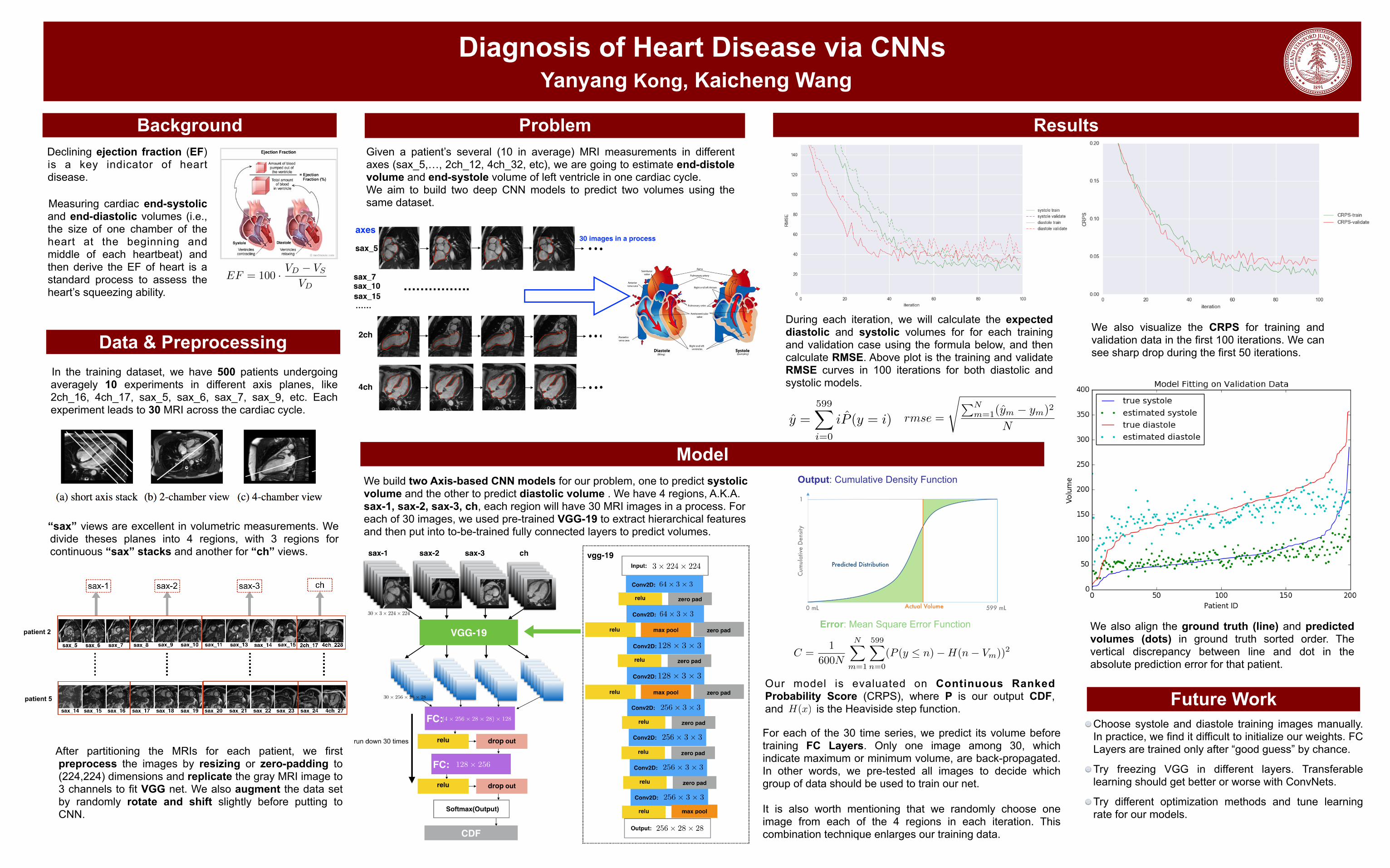
We also align the ground truth (line) and predicted volumes (dots) in ground truth sorted order. The vertical discrepancy between line and dot in the absolute prediction error for that patient.

For each of the 30 time series, we predict its volume before training FC Layers. Only one image among 30, which indicate maximum or minimum volume, are back-propagated. In other words, we pre-tested all images to decide which group of data should be used to train our net.

It is also worth mentioning that we randomly choose one image from each of the 4 regions in each iteration. This combination technique enlarges our training data.

patient 2

patient 5

Output: Cumulative Density Function

Error: Mean Square Error Function

C =1

600N

NX

m=1

599X

n=0

(P (y n)�H(n� Vm))2

During each iteration, we will calculate the expected diastolic and systolic volumes for for each training and validation case using the formula below, and then calculate RMSE. Above plot is the training and validate RMSE curves in 100 iterations for both diastolic and systolic models.

rmse =

sPNm=1(ym � ym)2

Ny =599X

i=0

iP (y = i)

We also visualize the CRPS for training and validation data in the first 100 iterations. We can see sharp drop during the first 50 iterations.

Our model is evaluated on Continuous Ranked Probability Score (CRPS), where P is our output CDF, and is the Heaviside step function.H(x)