water resources of the black sea basin at high spatial and ... · vest index. the harvest index is...

$: Water resources of the Black Sea Basin at high spatial and ... · vest index. The harvest index is a fraction of the above-ground plant dry biomass removed as dry yield. Plant growth$
RESEARCH ARTICLE10.1002/2013WR014132

Water resources of the Black Sea Basin at high spatial andtemporal resolutionElham Rouholahnejad1,2, Karim C. Abbaspour1, Raghvan Srinivasan3, Victor Bacu4,and Anthony Lehmann5

1Eawag, Swiss Federal Institute of Aquatic Science and Technology, Duebendorf, Switzerland, 2ETH Z€urich, Institute ofTerrestrial Ecosystem, Zurich, Switzerland, 3Texas A&M University, Texas Agricultural Experimental Station, Spatial ScienceLaboratory, College Station, Texas, USA, 4Department of Computer Science, Technical University of Cluj-Napoca, Cluj-Napoca, Romania, 5Climatic Change and Climate Impacts, University of Geneva, Carouge, Switzerland

Abstract The pressure on water resources, deteriorating water quality, and uncertainties associated withthe climate change create an environment of conflict in large and complex river system. The Black Sea Basin(BSB), in particular, suffers from ecological unsustainability and inadequate resource management leadingto severe environmental, social, and economical problems. To better tackle the future challenges, we usedthe Soil and Water Assessment Tool (SWAT) to model the hydrology of the BSB coupling water quantity,water quality, and crop yield components. The hydrological model of the BSB was calibrated and validatedconsidering sensitivity and uncertainty analysis. River discharges, nitrate loads, and crop yields were used tocalibrate the model. Employing grid technology improved calibration computation time by more than anorder of magnitude. We calculated components of water resources such as river discharge, infiltration, aqui-fer recharge, soil moisture, and actual and potential evapotranspiration. Furthermore, available waterresources were calculated at subbasin spatial and monthly temporal levels. Within this framework, a com-prehensive database of the BSB was created to fill the existing gaps in water resources data in the region. Inthis paper, we discuss the challenges of building a large-scale model in fine spatial and temporal detail. Thisstudy provides the basis for further research on the impacts of climate and land use change on waterresources in the BSB.

1. Introduction

The pressures on water resources and increasing conflict of interest present a huge water managementchallenge in the Black Sea Basin (BSB) [Global International Waters Assessment (GIWA), 2005]. The small-scalesectoral structure of water management is now reaching its limits. The integrated management of water inthe Basin requires a new level of consideration where water bodies are to be viewed in the context of thewhole river system and managed as a unit within their basins. This is of key interest for efficient and tar-geted water management through regional coordination, transparent balancing of interests, and clear prior-ity setting [Water Agenda 21, 2011]. A frequently advocated approach is to have adequate knowledge oftemporal and spatial variability of the fresh water availability and water quality [United Nations EnvironmentProgram (UNEP), 2006].

The BSB is internationally recognized for its ecologically unsustainable development and inadequateresource management leading to severe environmental, social, and economical problems. In 1995, it wasrated as being of the highest concern in five out of seven environmental categories, making it the worst ofany of the European seas [Stanners and Boudreau, 1995]. In another study, the German Advisory Council onGlobal Change (WBGU) states that the Black Sea is likely to experience (i) a degradation of freshwaterresources; (ii) an increase of storm and flood disasters; (iii) a decline in food production; and (iv) environ-mentally induced migration [Wissenschaftlicher Beirat Globale Umweltver€anderung (WBGU), 2007]. In addition,transboundary pollution effects (TPE) can be seen with respect to all economic sectors. Transboundary pol-lution is the pollution that originates in one country but causes damage in another country’s environment,by crossing borders in the rivers [Paleari, 2005].

Furthermore, the Intergovernmental Panel on Climate Change [IPCC, 2007] predicts important changes inthe coming decades that will not only modify climate patterns in terms of temperature and rainfall, but will

Key Points:� A high-resolution hydrological model

of the Black Sea Basin is built� We included river discharge, crop

yield, and nitrate load in calibration� Blue and green water resources of

the Basin are calculated at subbasinlevel

Correspondence to:E. Rouholahnejad,[email protected]

Citation:Rouholahnejad, E., K. C. Abbaspour, R.Srinivasan, V. Bacu, and A. Lehmann(2014), Water resources of the BlackSea Basin at high spatial and temporalresolution, Water Resour. Res., 50,doi:10.1002/2013WR014132.

Received 16 MAY 2013

Accepted 24 JUN 2014

Accepted article online 30 JUN 2014

ROUHOLAHNEJAD ET AL. VC 2014. American Geophysical Union. All Rights Reserved. 1

Water Resources Research

PUBLICATIONS

http://dx.doi.org/10.1002/2013WR014132

http://onlinelibrary.wiley.com/journal/10.1002/(ISSN)1944-7973/

http://publications.agu.org/

also drastically change freshwater resources qualitatively and quantitatively. This is expected to lead tomore floods or droughts in different regions, lowering of drinking water quality, increased risk of water-borne diseases, and irrigation problems. These changes may trigger socio-economic crises that need to beaddressed well in advance of the events in order to reduce the associated risks.

Previous research, which addressed water quantity and water quality in the BSB, includes a few global andregional studies. WaterGAP2 [Alcamo et al., 2003; D€oll et al., 2003] is a global model for water availabilityand water use. This model focuses on the global hydrology at grid scale (30 arc min) considering 3565major basins in the world with the drainage areas greater than 2500 km2. The model was initially used toestimate the water availability and demand and provides relatively limited water cycle-related components.In WaterGAP3 [Aus der Beek et al., 2012], a regional version of WaterGAP2, the hydrological fluxes draininginto Mediterranean and Black Sea were modeled with improved spatial resolution (5 arc min), snow melt,and water use. However, results using WaterGAP3 and WaterGAP2 are not significantly different in the BSB[Aus der Beek et al., 2012]. In a different approach, Meigh et al. [1999] developed a grid-based model GlobalWater Availability Assessment (GWAVA) to predict water resources scarcity at continental and global scales.This model has recently been further developed to include water quality [Dumont et al., 2012]. Using a sta-tistical approach, Grizzetti et al. [2008] assessed nitrogen content of surface water for major European riverbasins. Furthermore, discharges of water and nutrient to the Mediterranean and Black Sea are reported in astudy by Ludwig et al. [2009] for major rivers.

Next to the above mentioned studies, there are a few other investigations on the status of river basins inthe BSB [Sukhodolov et al., 2009; Sommerwerk et al., 2009; Wolfram and Bach, 2009]. However, often averageloads entering the Sea are reported without adequate spatial and temporal resolution on the current andfuture freshwater availability for the entire BSB. General shortcomings of the previous studies are missingdetail information on model inputs and outputs, unavailability of their input data, coarse spatial resolutionand scale of the models, and missing model calibration/validation and uncertainty analysis components.

In recent years, improvements in integrated hydrological modeling, advancements in calibration and uncer-tainty analysis tools, and availability of grid technology for model execution allow building more detailedand holistic models. These models account for processes such as water quantity and quality, soil, climate,land use, agricultural managements, and nutrient cycling in a coupled single package. The aim of the pro-ject is to build a high-resolution model of the entire BSB and to look at the impact of land use and climatechange on the water resources. The reason for building a single model of the BSB is to have a uniformly cali-brated model of the region rather than several disparately calibrated models. A high-resolution large-scalemodel has the advantages of allowing a holistic look at the Basin while retaining the small-scale system var-iabilities. The objectives of the current study are to: (i) gather and share a comprehensive database of theBSB, (ii) model the hydrology of the entire BSB by including agricultural management and crop yield to bet-ter quantify water quantity and water quality at daily time step and subbasin level, (iii) calibrate and validatethe model with uncertainty analysis using grid technology, (iv) produce a relatively accurate picture of waterresources availability, reliability, and pressures in the Basin.

To achieve the objectives of this research, we used the program Soil and Water Assessment Tool (SWAT)[Arnold et al., 1998]. SWAT was used because it is a continuous time and spatially distributed watershedmodel, in which hydrological processes and water quality are coupled with crop growth and agriculturalmanagement practices. The program was successfully applied in a wide range of scales and environmentalconditions [Gassman et al., 2007]. Another advantage of SWAT is its modular implementation where differ-ent processes can be selected.

For calibration and uncertainty analysis in this study, we used the Sequential Uncertainty Fitting programSUFI-2 [Abbaspour et al., 2004, 2007]. SUFI-2 is a tool for sensitivity analysis, multisite calibration, and uncer-tainty analysis. It lends itself easily to parallelization and is capable of analyzing a large number of parame-ters and measured data from many gauging stations (outlets) simultaneously. SUFI-2 is linked to SWAT inthe SWAT-CUP software [Abbaspour, 2011]. Yang et al. [2008] found that SUFI-2 needed the smallest numberof model runs to achieve a similarly good calibration and prediction uncertainty results in comparison withfour other techniques. This efficiency is of great importance when dealing with computationally intensive,complex large-scale models. We ran parallelized SUFI-2 on grid system described by Rouholahnejad et al.[2012] and Gorgan et al. [2012].

Water Resources Research 10.1002/2013WR014132


2. Material and Methods

2.1. Study AreaThe Black Sea Basin (Figure 1) with a total area of 2.3 3 106 km2 drains rivers of 23 European and Asiancountries (Austria, Belarus, Bosnia, Bulgaria, Croatia, Czech Republic, Georgia, Germany, Hungary, Moldova,Montenegro, Romania, Russia, Serbia, Slovakia, Slovenia, Turkey, Ukraine, Italy, Switzerland, Poland, Albania,and Macedonia) to the Black Sea. The Basin is inhabited by a total population of around 160 million people[Black Sea Investment Facility (BSEI), 2005]. It is mountainous in the east and south, in the Caucasus, and inAnatolia, and to the northwest with the Carpathians in the Ukraine and Romania. Most of the rest of theBlack Sea’s western and northern neighborhood is low lying. Mean annual air temperature shows a distinctnorth-south gradient from <23�C to >15�C. The precipitation pattern is characterized by a west-east gradi-ent from a high of >3000 mm yr21 to a low of <190 mm yr21 [Tockner et al., 2009]. The dominant land usein the basin is agricultural with 65% of coverage according to MODIS Land Cover [NASA, 2001]. Major riversdraining into the Black Sea include Danube, Dnieper, and Don. The greatest sources of diffuse pollution areagricultural and households not connected to sewer systems [European Environmental Agency (EEA), 2010].

2.2. Soil Water Assessment Tool (SWAT)SWAT was used to simulate hydrology, water quality, and vegetation growth in BSB. SWAT is a process-based, semidistributed, hydrologic model. The model has been developed to quantify the impact of landmanagement practices on water, sediment, and agricultural chemical yields in large complex watershedswith varying soils, land uses, and management conditions over long periods of time. SWAT was chosenbecause of the close linkage between its development purposes and the objectives of this project, openaccess to the source code, and its successful application in a wide range of scales and environmentalconditions.

The main components of SWAT are hydrology, climate, nutrient cycling, soil temperature, sediment move-ment, crop growth, agricultural management, and pesticide dynamics. SWAT is a continuous simulationmodel operating on a daily time step. The spatial heterogeneity of the watershed is preserved by topo-graphically dividing the basin into multiple subbasins. These are further subdivided into hydrologicresponse units (HRU) based on soil, land use, and slope characteristics. These subdivisions enable the modelto reflect differences in evapotranspiration for various crops and soils. In each HRU and on each time step,the hydrologic and vegetation-growth processes are simulated based on the curve number rainfall-runoffpartitioning and the heat unit phenological development method [Neitsch et al., 2009].

Figure 1. Illustration of Black Sea Basin showing major rivers and measured stations of climate, discharge, and nitrate. Also shown is thecomparison of observed and simulated discharge and nitrate using the efficiency criterion bR2. The six large river basins of Danube,Dnieper, Don, Kuban, Kizilirmak, and Sakarya are highlighted.



Runoff is predicted separately for each HRU and routed to obtain the total model runoff for the watershed.The routing phase of the hydrologic cycle in SWAT is the movement of water, nitrate, etc., through thechannel network of the watershed. Once SWAT determines the loadings of water, sediment, nutrients, andpesticides to the main channel, the loadings are routed through the stream network of the watershed. Inaddition to keeping track of mass flow in the channel, SWAT models the transformation of chemicals in thestream and streambed.

Energy availability governs vegetation phenology. At each point in the growth cycle, biomass production isderived from the interception of solar radiation by leaves, plant-specific radiation use efficiency, and leafarea index (LAI). Crop yield is calculated at harvest by multiplying the above-ground biomass with the har-vest index. The harvest index is a fraction of the above-ground plant dry biomass removed as dry yield.Plant growth is limited by temperature, water, and nutrient availability in the soil and is influenced by agri-cultural management (e.g., fertilization, irrigation, and timing of operations). A detailed description ofSWAT’s theory can be obtained in Neitsch et al. [2009].

2.3. Input Data and Model OutputsBSB Digital Elevation Model (DEM) at 90 m spatial resolution was extracted from SRTM [Jarvis et al., 2008].The river network data set was from European Catchments and Rivers Network System [EEA Catchmentsand Rivers Network System (ECRINS) v1.1, 2012]. The ECRINS river map was corrected in the areas where therewas a mismatch with DEM to achieve a correct flow direction.

The soil data were obtained from the FAO-UNESCO global soil map [Food and Agricultural Organization(FAO), 1995], which provides data for 5000 soil types comprising two layers (0–30 cm and 30–100 cm depth)at a spatial resolution of 5 km.

Four different land uses were available for the region: (i) Global Land Cover Characterization (GLCC) at 1 kmspatial resolution [U. S. Geological Survey (USGS), 2008], (ii) MODIS land cover with spatial resolution of500 m [NASA, 2001], (iii) GlobCover with spatial resolution of 300 m [Environmental Space Agency (ESA),2008], (iv) Global Corine at 300 m spatial resolution [Environmental Space Agency (ESA), 2010].

Two different climate databases were available: measured and gridded data. Measured climate included456 rainfall and 678 temperature stations mainly collected from National Climatic Data Centre (NCDC;http://www.climate.gov/#dataServices/dataLibrary), the European Climate Assessment and Dataset (ECAD)[Haylock et al., 2008], Turkish Ministry of Forest and Water Affairs (MEF), and Romanian National Institute ofHydrology and Water Management (INHGA) for the period of 1970–2008. Only stations with <20% missingdata were included in the model. Gridded data are constructed from measured climate stations and inter-polated to grid resolution. We used data from Climate Research Units [Climatic Research Unit (CRU), 2008;Mitchell and Jones, 2005] at 0.5� resolution amounting to 1147 grid points. The daily global solar radiationdata were obtained from 6110 virtual stations at 0.5� resolution for the duration of 1960–2001 [Weedonet al., 2011].

Monthly river discharge data for model calibration and validation were obtained from Global Runoff DataCenter [Global Runoff Data Centre (GRDC), 2011], National Institute of Hydrology and Water Management(INHGA) and Danube Delta National Institute for Research and Development (DDNI) in Romania, and TurkishMinistry of Forest and Water Affairs (MEF) for the period 1970–2008. Only stations with <20% missing dataand minimum length of 5 years were included in calibration-validation process. This led to 144 dischargeoutlets where 37 of them also contained nitrate data from International Commission for the Protection ofthe Danube River (ICPDR). These outlets had differing beginning and ending time periods.

Point sources were also assigned to each subbasin in the model. The nutrient loads of subbasins were calcu-lated based on the population of the subbasins, the percentage of population connected to wastewatertreatment plant, and the average rate of nitrogen per population equivalent. Population percentage con-nected to any kind of sewage treatment was derived from Eurostat for the period of 2000–2009. This sharewas above 80% in approximately half of the European Union countries for which data are available, risingto 95% in Germany. At the other end, less than one in two households were connected to urban wastewatertreatment in Bulgaria and Romania. In terms of treatment levels, tertiary wastewater treatment was mostcommon in Germany, Austria, and Italy where at least four in every five persons were connected to thistype of wastewater treatment. In contrast, no more than 1% of the population was connected to tertiary



http://www.climate.gov/#dataServices/dataLibrary

wastewater treatment in Romania and Bulgaria. We assumed the treatment efficiency to be 80% in all coun-tries with 20% loading directly into surface waters and hence considered as point sources.

To account for industrial and household releases, Zessner and Lindtner [2005] calculated the nitrogen loadto be 8.8 g N P21

e d21, where Pe is population equivalent, which is the number expressing the ratio of thesum of the pollution load produced during 24 h by industrial facilities and household to the individual pol-lution load in household sewage produced by one person in the same time. The ratio of population and Pe

varies in a way that 80% of the treatment plants lie in the range of 0.4–0.9. The average value of this ratio isassumed to be 0.63 [Zessner and Lindtner, 2005]. The nutrient load is calculated as

LN5PeIN 12Srateð Þ1 12Teffð ÞSrate½ � (1)

where LN is the nitrogen load entering rivers in subbasins (g d21), Teff is the wastewater treatment efficiency,IN is the average input of nitrogen from household to wastewater (g N P21

e d21), and Srate is the percentageof the population connected to any kind of sewage treatment. We used population map of year 2005 fromthe Center for International Earth Science Information Network in 2.5 arc min resolution [Center for Interna-tional Earth Science Information Network (CIESIN), 2005] and extrapolated to other years based on thenational population growth rate provided by the World Bank.

Cropping area and the start and end month of cropping periods in the BSB countries were derived fromMIRCA2000 database on global monthly irrigated and rain-fed cropping areas around the year 2000 (5 yearaverage), at a spatial resolution of 5 arc min [Portmann et al., 2010]. This database represents multicroppingsystems and maximizes consistency with census-based national and subnational statistics. Crop yield datawere obtained from McGill University [Monfreda et al., 2008] at 5 min resolution. This data were 5 year aver-ages around the year 2000 and were used to calculate per subbasin crop yields for maize, barley, andwheat. Country-based crop yield was obtained from FAOSTAT database [Food and Agricultural OrganizationStatistics (FAOSTAT), 2013].

SWAT produces a large amount of output variables. In this study we look at the water cycle components,crop yield, and nitrate concentration in rivers. Using the water cycle constituents calculated in SWAT, wecould also calculate water resources components such as ‘‘blue water,’’ ‘‘green water flow,’’ and ‘‘green waterstorage.’’ Currently, the definition of blue water is generally accepted as the sum of the river discharge andthe deep groundwater recharge. This is in essence the water resources by the traditional hydrological andengineering definition. There exist slightly different definitions for the term green water. Falkenmark andRockstrom [2006] differentiate between the green water ‘‘resource’’ and the green water ‘‘flow.’’ Accordingto their definition, green water resource is the moisture in the soil, which is a renewable resource and canpotentially generate economic returns, as it is the source for rain-fed agriculture. The green water flow iscomposed of the actual evaporation (the nonproductive part) and the actual transpiration (the productivepart), commonly referred to together as the actual evapotranspiration.

2.4. Model SetupThe subbasins were delineated with a threshold area of 100 km2 yielding 12,982 subbasin. This was thesmallest threshold that could be used to build the ArcSWAT project on a 64 bit laptop with 2.7 GHz process-ors, 4 cores, 8 GB of RAM, and Windows7 operating system. This is because of memory limitation and ineffi-ciency of ArcGIS in handling large raster calculation. In addition, the personal geodatabase of ArcSWATcreated by ArcGIS9 has a limitation of 2 GB on the file size. Fourteen different land cover classes of MODISwere assigned to land uses in the SWAT database. Subsequently, each of the 12,982 subbasins was spiltinto unique combinations of slope, land use classes, and soil types resulting in 89,202 Hydrologic ResponseUnit (HRU). Three classes of slope (0–3%, 3–6%, and >6%) were used in the subbasin discretization. We alsoused five elevation bands in each subbasin to adjust for orographic change in temperature (26�C km21)and precipitation (670 mm km21) after some initial fitting.

Twenty-five different management plans were designed based on the crop types, cropping dates, winter orsummer crops, irrigated or rain-fed applications. Each HRU then corresponded to a management plan.Exclusive agricultural classes were assigned to each country so that desired management could be definedat the national level. Subsequently, agricultural areas within these classes were subdivided proportional tothe cropping areas of irrigated/rain-fed, winter/spring types for wheat, maize, and barely. The three major



crops were allocated to agricultural lands in MODIS proportional to their contribution in each country’s har-vested areas as reported by MIRACA2000 [Portmann et al., 2010].

The option of automatic fertilization in SWAT was employed to meet crop need and the annual maximumapplication amount was set to 300 kg N ha21. This assumption leads to underestimation of nitrogen in areaswhere application is more than crop need. Elemental nitrogen and elemental phosphors were applied tothe agricultural lands in each subbasin as the main fertilizer in BSB. An additional nitrogen input of 1.2 mgN l21 was assumed in the rainfall. It is notable that in the MODIS classification agricultural land does notinclude permanent grassland.

We invoked automatic irrigation based on plant water demand in such a way as to minimize crop waterstress in irrigated lands. In this study, potential evapotranspiration (PET) was estimated using the Hargreavesmethod [Hargreaves et al., 1985] while actual evapotranspiration (ET) was estimated based on Ritchie [1972].

The simulation period was 1970–2006 using 3 years of initialization (1970–1972) as warm up period. Aseach station had a different beginning and ending time periods, the model was calibrated from 1973 to1996 and validated from 1997 to 2006 for discharge, and because of fewer data in the early years, thenitrate loads were calibrated from 1973 to 2000 and validated from 2001 to 2006. Within these generalyears different stations had different data availability periods. Given the disparity in data lengths andtiming, this was the most sensible division of data between calibration and validation time period.SWAT always runs on daily time step, but we used monthly outputs for calibration and validation of themodel. Using SWAT 2009, it took 42 h for a single-model run on the laptop where ArcSWAT project wasbuilt.

2.5. Model Calibration ProcedureSensitivity, calibration, validation, and uncertainty analysis were performed for water quantity, water qual-ity, and crop yield using river discharges, nitrate loads in rivers, and yields of wheat, barley, and maize.SUFI-2 was used for calibration and uncertainty analysis. In SUFI-2, all sources of uncertainties are mappedto a set of parameter ranges. They are calibrated with the dual aim of bracketing most of the observeddata with as narrow as possible uncertainty band. Initially, a set of meaningful parameter ranges areassigned to calibrating parameters based on literature, knowledge of site processes, and sensitivity analy-ses. Then a set of Latin hypercube samples are drawn from the parameter ranges, and the objective func-tion is calculated for each parameter set. The uncertainty is quantified at the 2.5% and 97.5% levels of thecumulative frequency distribution of all simulated output values, and it is referred to as the 95% predic-tion uncertainty (95PPU). The lower, middle, and upper boundaries of the 95PPU (L95PPU, M95PPU, andU95PPU) reflect the 2.5, 50, and 97.5 percentiles of the distribution, respectively. Values at the 50% proba-bility level are used for drawing average long-term maps of different variables. The goodness of modelperformance in terms of calibration and uncertainty level is evaluated using the P-factor and the R-factorindices. The P-factor is the percentage of measured data bracketed by the 95PPU band. It ranges from 0to 1 where 1 is ideal and means all of the measured data are within the uncertainty band (i.e., model pre-diction). The R-factor is the average width of the band divided by the standard deviation of the measuredvariable. It ranges from 0 to1 where 0 reflects a perfect match with the observation. Based on the expe-rience, an R-factor of around 1 is usually desirable [Abbaspour et al., 2007] where the thickness of theuncertainty band does not exceed the measured standard deviation. SUFI-2 allows for a measurementerror of about 10% to be assigned to all observed variables, which are accounted for in the 95PPUcalculations.

Coefficient of determination r2 is a measure of dispersion around the mean of the observed and predictedvalues and can be used as an efficiency criteria. The range of r2 lies between 0 and 1 which describes howmuch of the observed dispersion is explained by the prediction. A value of zero means no correlation at allwhereas a value of 1 means that the dispersion of the prediction is equal to that of the observation. Thefact that only the dispersion is quantified is one of the major drawbacks of r2 if it is considered alone. Amodel which systematically over or underpredicts all the time will still result in good r2 values close to 1.0even if all predictions were wrong. By weighting r2 by the slope of regression line between observed andpredicted, under or overpredictions are quantified together with the dynamics which results in a more com-prehensive reflection of model results. We used a slightly modified weighted r2 as originally introduced byKrause et al. [2005] as the efficiency criterion for discharge and nitrate



u5jbjr2 for jbj � 1

jbj21r2 for jbj > 1

((2)

where r2 is the coefficient of determination and b is the slope of the regression line between the simulatedand measured data. For a good agreement the interception of the regression line should be close to zerowhich means that an observed runoff of zero would also result in a prediction near zero and the gradient bshould be close to one. For multiple outlets and attributes, the objective function U was expressed as

H51

wv11wv2

wv1Xn1

i51

wi

Xn1

i51

wi/i1wv2Xn2

i51

wi

Xn2

i51

wi/i

266664

377775 (3)

where wv1 and wv2 are weights of the two variables, n1 and n2 are the number of discharge and nitrate sta-tions, respectively, and wi’s are the weights of variables at each station. The function / and consequently Hvary between 0 and 1. The best simulation is considered the one with the highest H value. A major advant-age of br2 efficiency criterion is that it ranges from 0 to 1, which compared to Nasch-Sutcliff Efficiency coeffi-cient, ensures that in a multisite multiattribute calibration, the objective function is not dominated by a fewbad results. Weights in equation (3) would be critical if an objective function such as mean square error wasused, but because of using br2 they did not make any significant difference to model calibration results. Forthis reason, we set them to 1. For crop yield we used mean square error as the objective function after aninitial calibration of model for discharge and nitrate

/351

n3

Xn3

i51

Yoi 2Ys

i

� �2(4)

where n3 is the number of sites with wheat, barley, and corn yield data, Yo (t ha21) is the observed yield,and Ys (t ha21) is the simulated yield.

A few iterations are then carried out seeking to reach an optimal P-factor and R-factor until a furtherimprovement in the objective function is not found. As mentioned before, the calibration runs were madeusing parallel SUFI-2 [Rouholahnejad et al., 2012] and the grid-based SWAT (gSWAT) [Gorgan et al., 2012]. AsSUFI-2 is a sequential procedure, several iterations of 200 simulations each were performed for calibration.

3. Results and Discussion

The model response to various land uses and climate data was tested by comparing simulated river dis-charges against the observation. For land use, our analysis indicated that classification and resolution didnot have a significant effect on river discharge simulation in the BSB model. MODIS land cover was used inthe final SWAT project as it produced relatively better discharge results. As model calibration started farback in time, we also tested the model by changing the land use during SWAT simulation. We found thatthe impact of historic land use change on our large-scale model results was negligible and, hence, did notconsider this change during calibration.

We also found that CRU-based simulated discharges performed significantly better in the project as com-pared to simulated discharges based on measured climate stations. This could be because the climate sta-tions suffered from a large amount of missing data, different data qualities, and uneven distributionthroughout the region. Subsequently, the CRU data set was selected to model the hydrology of the BSB.

SWAT calculates the rainfall and temperature of each subbasin using the nearest climate station to the cent-roid of that subbasin. As rainfall is the most important driving variable in a hydrological model, when com-paring the results of this work with other works, it is important to have the distribution of the rainfall inmind (Figure 2). Differences are observed in the coefficients of variation (CV) of long-term annual precipita-tion and temperature averages (1973–2006) across the BSB. This indicates the degree of year to year



variability during the simulation period. This variation has an influence on the prediction uncertainties of allwater cycle components as we will see later for the case of Bulgaria and Turkey.

3.1. Calibration and Uncertainty Analysis3.1.1. Examining Model SetupInitially, a broad set of parameters were used for discharge calibration [Holvoet et al., 2005; Wang et al., 2005,Abbaspour et al., 2007; Faramarzi et al., 2009]. Then a sensitivity analysis was performed to identify the keyparameters across BSB, which led to selection of 20 parameters integrally related to stream flow (Table 1).Although the initial parameter ranges were as wide as physically meaningful, some outlets were still com-pletely outside of the 95PPU range. These outlets would obviously not benefit from parameter calibrationalone. We investigated the poorly simulated outlets one by one using the visualization module of SWAT-CUP. This involves projection of the study area on the Microsoft’s BING map to identify the reasons for theinadequate simulations. In the visualization module, we observe the subbasins, outlet positions, simulatedrivers, and climate stations from the SWAT project, as well as landcover and other layers of information inthe BING map. Several problems were discovered, which are inevitable in a large-scale projects and neededcareful attention.

Examples of these include positioning the outlets on a wrong rive (Figures 3a and 3b). As SWAT connectseach measured outlet to the nearest rivers, any errors in the coordinates of outlets can cause a wrong

Figure 2. Long-term annual average (1973–2006) precipitation and average temperature distribution across Black Sea Basin based on the CRU data set. Also shown are the coefficientsof variation indicating the temporal variability of precipitation and average temperature.



placement. This perhaps leads to the biggest calibration problem. As shown in Figure 3b, the outlet isplaced on a tributary of the Danube called Tamis near Pancevo in Serbia. The black dashed line near the xaxis (Figure 3c) is simulated river discharge before correcting the location, and the red line shows simulateddischarge after correcting the location.

Other major problems result from an outlet being positioned downstream of a reservoir. In particular, inSouthern Bug in Ukraine, the simulated discharge and observations match quite well until the Alexandra

0

3000

6000

9000

12000

15000

Dis

ch

arg

e (

m3

s-1) Obs

Sim. before reposi�oning (Sub 10565)

Sim a�er reposi�oning (Sub 10624)

a b

c

Figure 3. Example of a wrong positioning of the outlets due to errors in the reported coordinates of the measurement stations. The out-let’s correct position is on the Danube River (upstream area of 497,500 km2) rather the Tamis River (upstream area of 16,460 km2), a tribu-tary of the Danube.

Table 1. List of Parameters and Their Initial Ranges Used for Model Calibration

Parameter Name Definition Initial Range

r__CN2.mgt SCS runoff curve number for moisture condition II 20.35 to 0.35r__ALPHA_BF.gw Base flow alpha factor (days) 20.8 to 0.8r__GW_DELAY.gw Groundwater delay time (days) 20.8 to 0.8r__GWQMN.gw Threshold depth of water in shallow aquifer for return flow (mm) 20.8 to 0.8r__GW_REVAP.gw Groundwater revap. coefficient 20.4 to 0.4r__REVAPMN.gw Threshold depth of water in the shallow aquifer for ‘‘revap’’ (mm) 20.4 to 0.4r__RCHRG_DP.gw Deep aquifer percolation fraction 0.3 to 0.5r__CH_N2.rte Manning’s n value for main channel 20.8 to 0.8r__CH_K2.rte Effective hydraulic conductivity in the main channel (mm h21) 20.8 to 0.8r__ALPHA_BNK.rte Base flow alpha factor for bank storage (days) 20.6 to 0.6r__SOL_AWC().sol Soil available water storage capacity (mm H2O/mm soil) 20.5 to 0.5r__SOL_K().sol Soil conductivity (mm h21) 20.8 to 0.8r__SOL_BD().sol Soil bulk density (g cm23) 20.4 to 0.4r__SFTMP().sno Snowfall temperature (�C) 20.4 to 0.4r__SMTMP().sno Snow melt base temperature (�C) 20.4 to 0.4r__SMFMX().sno Maximum melt rate for snow during the year (mm �C21 d21) 20.4 to 0.4r__SMFMN().sno Minimum melt rate for snow during the year (mm �C21 d21) 20.4 to 0.4r__SLSUBBSN.hru Average slope length (m) 20.4 to 0.4r__OV_N.hru Manning’s n value for overland flow 20.4 to 0.4r__HRU_SLP.hru Average slope steepness (m m21) 20.4 to 0.4r__CMN.bsn Rate factor for humus mineralization of active organic nitrogen 20.4 to 0.4r__NPERCO.bsn Nitrogen percolation coefficient 20.4 to 0.4r__N_UPDIS.bsn Nitrogen uptake distribution parameter 20.4 to 0.4r__RCN.bsn Concentration of nitrogen in rainfall (mg N L21) 20.4 to 0.4r__SHALLST_N.gw Concentration of nitrate in groundwater to streamflow (mg N L21) 20.4 to 0.4



Reservoir came into operation in 1979 (Figure 4). Clearly the dynamics of such outlets depend on the man-agement of the reservoir and not natural processes. Other problematic situations may arise when outletsare in a highly populated or agricultural region where water management and water transfers are large. Inthese situations also, SWAT cannot be expected to produce proper results unless data are available. Con-structions of dams for irrigation and power generation purposes as well as other water management prac-tices such as water abstraction and diversion create major difficulties for model calibration. As managementinformation are usually not available, proper cautions need to be taken during calibration. These includeconverting outlets to inlets, weighing those outlets under the influence of management less in the objectivefunction, or removing the outlets downstream of reservoirs from the calibration process. Because of lack ofwater management data, we excluded from calibration those outlets directly affected by infrastructuressuch as dams and reservoirs. After making appropriate corrections to badly simulated outlets and obtainingrelatively satisfactory discharge estimation, nitrate parameters (Table 1) were added to the parameter pool.

3.1.2. ParameterizationIn subsequent iterations the model was parameterized. Parameterization refers to regionalization of param-eters tailored to achieve the best response from the simulation program and individual outlets. Some exam-ples are if there is an early shift in the simulation (Figure 5a), then decreasing the overland flow (HRU_SLP)by 10–20%, increasing Manning’s roughness coefficient (OV_N) by 10–30%, and increasing the flow length(SLSUBBSN) by 5–15 m in all the upstream subbasins of that outlet will improve the simulated discharge.Accordingly, if the simulated base flow is too high (Figure 5b), then parameterization includes: increasingdeep percolation loss (GWQMN), increasing groundwater revap coefficient (GW_REVAP) to a maximum of0.4, and decreasing the threshold depth of water in shallow aquifer (REVAPMN) to a minimum of zero. Inanother example, if the simulated peak flow is underestimated (Figure 5c), then the following adjustmentsto the upstream subbasins of that outlet should be made: increasing the curve number (CN2) by 10–15%,decreasing the soil available water storage capacity (SOL_AWC) by 5–10%, and decreasing the soil evapora-tion compensation factor (ESCO) by 20–30%. This will ensure a better simulation at the specified outlet. Forevery outlet, the upstream subbasins were parameterized as described above.

3.1.3. Calibration PerformanceThe final calibration results for outlets that were used in model calibration range from very good to poor(Figure 1). The bR2 statistic for discharge outlets range from 0.2 to 0.8 and for nitrate outlets from less than0.1 to 0.7. The time series examples (Figure 6) for two outlets show good results in both calibration and vali-dation periods.

It is important to note that the 95PPU represents model prediction and not the ‘‘best simulation.’’ The latteris only provided for reference. Calibration is concerned with the problem of making inferences about physi-cal systems from measured output variables of the model (e.g., river discharge, nitrate load, etc.). Becausenearly all measurements are subject to some uncertainty, the inferences are usually statistical in nature. Fur-thermore, because one can only measure a limited number of (noisy) data and because physical systemsare usually modeled by continuum equations, no calibration problem is really uniquely solvable [Abbaspouret al., 2007]. In calibration, therefore, we characterize the set of models, mainly through assigning distribu-tions (uncertainties) to the parameters that fit the data. We should also make the distinction here between

0

200

400

600

800

1000

1200

Dis

ch

arg

e (

m3s

-1)

Observa�on

Simula�on

Figure 4. Example of an outlet being at the downstream of a reservoir. In the Southern Bug in Ukraine (upstream area of 45,180 km2), Alex-andra Reservoir came into operation in 1979. There is a clear change in the discharge pattern after the operation of the reservoir whichcould not be captured by the model.



0

100

200

300

400

Dis

ch

arg

e (

m3

s-1) Observa�on

Simula�on before parameteriza�on

Simula�on a�er parameteriza�on

0

200

400

600

800

1000

Dis

ch

arg

e (

m3

s-1) Observa�on



0

100

200

300

400

500

Dis

ch

arg

e (

m3

s-1) Observa�on



Example of a shi� in the simula�on (Vrona River, Russia, upstream area of 5270 km2

)

Example of low peak in the simula�on (Prut River, Romania, upstream area of 9101 km2

)

a

b

c

Example of high base flow in the simula�on (Tisza River, Hungary, upstream area of 26810 km2

)

Figure 5. Examples of parameterization. Simulations are discrepant in terms of a shift, higher base flow, or lower peaks. In each case, rele-vant parameters are changed in all the upstream subbasins.

0

1000

2000

3000

4000

Dis

ch

arg

e (

m3s

-1)

Prypiat draining to Danieper, Belarus, upstream area of 12360 km2

95 PPU

Obs

Best_Sim

0

100

200

300

400

500

600

700

Dis

ch

arg

e (

m3

s-1)

Prut; Romania, Moldova, Ukraine, upstream area of 9101 km2

95 PPU

Obs

Best_Sim

P-factor= 0.8

R-factor= 1.71

br2

= 0.44

NS= 0.28

P-factor= 0.59

R-factor= 0.92

br2

= 0.43

NS= 0.47

Cal.

Cal.

Val.

Val.

Figure 6. Comparison of simulated and observed discharges at Prypiat and Prut rivers for calibration and validation periods. The shadedregion is 95% prediction uncertainty band. The best model simulation is also shown by the red line. The reported statistics are for theentire simulation period.



uncertainty and error. Prediction uncertainty arises from the uncertainty in the parameters, in the model,and in the inputs. In the concept of SUFI-2, all these uncertainties are assigned to the parameter distribu-tions. The uncertainty is expressed as the 95PPU, which as stated above is also the output of the model (Fig-ure 6). Model error, however, is the degree in which the 95PPU does not account or does not bracket theobservation. This, in SUFI-2, is indicated by (1-P-fcator), which is around 20% for Daniper and 41% for PrutRiver (Figure 6). A closer examination of the Prut River simulation reveals that most of the error originatesfrom the base flow simulation. Hence, the processes related to surface water-ground water interaction arenot very well represented in the model in that region.

For a model to better represent a region of study we could introduce more attributes in the objective func-tion. In this research, we used nitrate load as well as crop yield to achieve a model with more confidence inpredicting the water balance components.

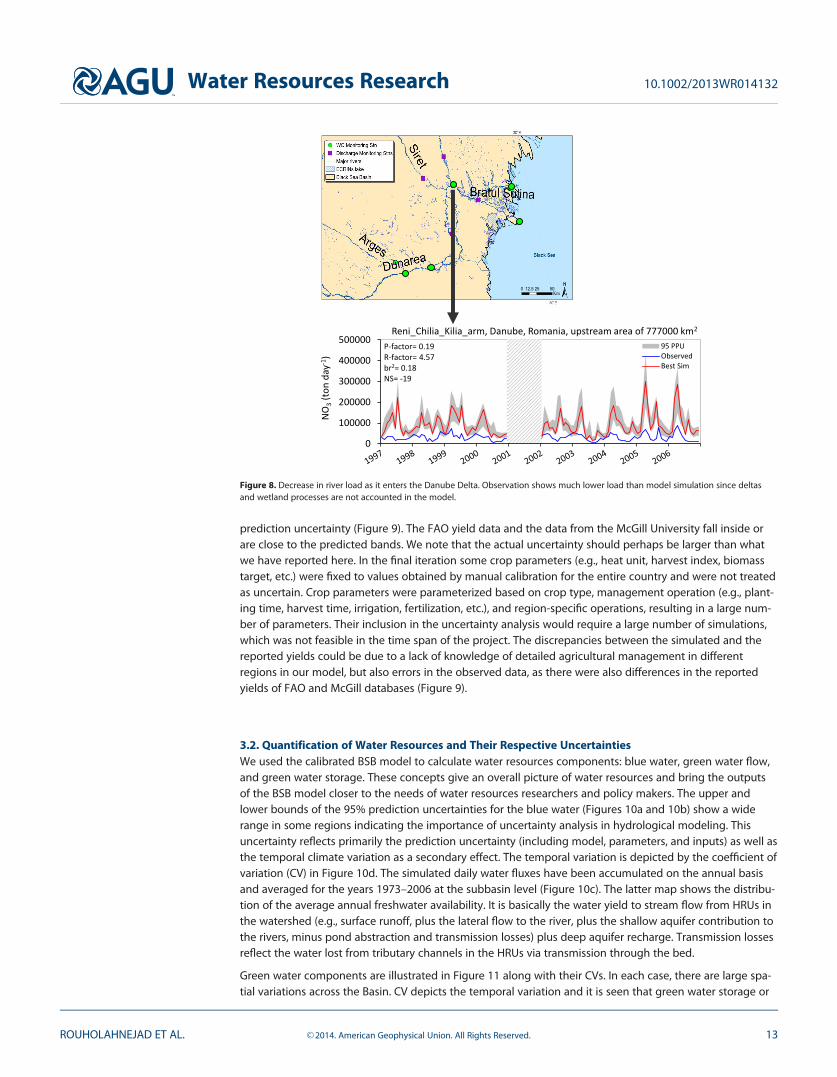
Water quality was simulated through nitrate loads in rivers. We were disappointed at the lack of more easilyavailable information in the BSB, especially with respect to water quality. Most of the information we gath-ered came from the Danube River Basin; therefore, the water quality component of the Black Sea modelshould be considered as uncalibrated or at best partially calibrated for other river basins within the BSB. Thesimulations, however, were surprisingly satisfactory for most stations given that we had estimated the pointsources and had only rough data with respect to diffuse sources of pollution in different countries (Figure 7).It is expected that nitrate simulation would be accompanied by much large prediction uncertainty due tolarger uncertainty in the input data for point and diffuse sources. An interesting observation is the overesti-mation of the model at the stations near Danube Delta. As the river approaches the Delta, the concentrationof nitrate decreases, but the model cannot account for this because deltas and wetlands are not representedin SWAT (Figure 8).

Because of a direct relationship between crop yield and evapotranspiration [Jensen, 1968; FAO, 1986], inaddition to nitrate loads, we included yields of maize, barley, and wheat as extra target variables in the cali-bration process. With measured river discharges we can obtain a good knowledge of runoff, but cannothave any confidence with respect to soil moisture, evapotranspiration, or aquifer recharge. Knowledge ofevapotranspiration through simulation of crop yield could, therefore, increase our confidence in soil mois-ture and aquifer recharge. Average annual yield of three major crops (barley, maize, and wheat) are simu-lated at subbasin level and aggregated per country for the duration of 1973–2006 and expressed as 95%

0

2000

4000

6000

8000

NO

3(to

n d

ay

-1)

Pohansko, Breclav, Czech Republic, upstream area of 12190 km2

95 PPU

Observed

Best Sim

0

10000

20000

30000

40000

50000

NO

3(to

n d

ay

-1)

Medvedof, Danube, Slovakia, upstream area of 128200 km2

95 PPU

Observed

Best Sim

P-factor= 0.54

R-factor= 1.8

br2

= 0.5

NS= 0.23

P-factor= 0.81

R-factor= 2.13

br2

= 0.44

NS= 0.25

Cal.

Cal.

Val.

Val.

Figure 7. Comparison of simulated and observed nitrate loads in Dyje River in Czech Republic and Danube River in Slovakia for calibrationand validation periods. The shaded region is 95% prediction uncertainty band. The best model simulation is also shown by the red line.The reported statistics are for the entire simulation period.



prediction uncertainty (Figure 9). The FAO yield data and the data from the McGill University fall inside orare close to the predicted bands. We note that the actual uncertainty should perhaps be larger than whatwe have reported here. In the final iteration some crop parameters (e.g., heat unit, harvest index, biomasstarget, etc.) were fixed to values obtained by manual calibration for the entire country and were not treatedas uncertain. Crop parameters were parameterized based on crop type, management operation (e.g., plant-ing time, harvest time, irrigation, fertilization, etc.), and region-specific operations, resulting in a large num-ber of parameters. Their inclusion in the uncertainty analysis would require a large number of simulations,which was not feasible in the time span of the project. The discrepancies between the simulated and thereported yields could be due to a lack of knowledge of detailed agricultural management in differentregions in our model, but also errors in the observed data, as there were also differences in the reportedyields of FAO and McGill databases (Figure 9).

3.2. Quantification of Water Resources and Their Respective UncertaintiesWe used the calibrated BSB model to calculate water resources components: blue water, green water flow,and green water storage. These concepts give an overall picture of water resources and bring the outputsof the BSB model closer to the needs of water resources researchers and policy makers. The upper andlower bounds of the 95% prediction uncertainties for the blue water (Figures 10a and 10b) show a widerange in some regions indicating the importance of uncertainty analysis in hydrological modeling. Thisuncertainty reflects primarily the prediction uncertainty (including model, parameters, and inputs) as well asthe temporal climate variation as a secondary effect. The temporal variation is depicted by the coefficient ofvariation (CV) in Figure 10d. The simulated daily water fluxes have been accumulated on the annual basisand averaged for the years 1973–2006 at the subbasin level (Figure 10c). The latter map shows the distribu-tion of the average annual freshwater availability. It is basically the water yield to stream flow from HRUs inthe watershed (e.g., surface runoff, plus the lateral flow to the river, plus the shallow aquifer contribution tothe rivers, minus pond abstraction and transmission losses) plus deep aquifer recharge. Transmission lossesreflect the water lost from tributary channels in the HRUs via transmission through the bed.

Green water components are illustrated in Figure 11 along with their CVs. In each case, there are large spa-tial variations across the Basin. CV depicts the temporal variation and it is seen that green water storage or

0

100000

200000

300000

400000

500000

NO

3(to

n d

ay

-1)

Reni_Chilia_Kilia_arm, Danube, Romania, upstream area of 777000 km2

95 PPU

Observed

Best Sim

P-factor= 0.19

R-factor= 4.57

br2= 0.18

NS= -19

0 25 5012.5Km

Figure 8. Decrease in river load as it enters the Danube Delta. Observation shows much lower load than model simulation since deltasand wetland processes are not accounted in the model.



soil moisture is relatively less variable temporally in many regions. This indicates a higher reliability of thisresource over time, and hence, a less risky opportunity for development of green, or rain-fed agriculture.

The confidence on water resources estimates is relatively high because surface runoff as well as evapotrans-piration (through crop yield) was satisfactorily calibrated in the model. For a further comparison with thereported literature we calculated the freshwater availability on country basis and compared them to the val-ues of FAO (Figure 12). The simulation results are expressed as 95% prediction uncertainty bands. It is seenthat the FAO-estimated water availability fall inside or are very close to the simulation 95PPU band in allcountries. Summary of water resources for major BS countries are presented in Table 2. Georgia is shown tohave the largest blue water in mm yr21, and Bulgaria the smallest.

Knowledge of the long-term time series of water availability is very important in water management andplanning studies, water transfers, reservoir operation, and conjunctive water analyses. Many countries havelarge monthly variabilities in the blue and green water components as illustrated, for example, by the long-term monthly variations in Turkey and Bulgaria (Figure 13). It is interesting to note that soil moisture (greenwater storage) is larger in Bulgaria than in Turkey, while Turkey’s blue water is larger. We could concludethat as a whole, runoff is larger in Turkey, while the share of infiltration is greater in Bulgaria. The largeuncertainty in green water storage in Bulgaria appears to be dominated by large annual variation in precipi-tation (Figure 2b).

3.3. Transboundary RiversAs measurements cannot be made at all transboundary points and for all variables, models can play animportant role. We use the example of Dniester River to show the ability of the model to address some

0

2

4

6

8

Yie

ld (

to

n h

a-1)

Barley

0

2

4

6

8

10

Yie

ld (

to

n h

a-1)

Maize

0

2

4

6

8

Yie

ld (

to

n h

a-1)

Wheat

Wheat yld, 95 PPU, SWAT Wheat yld, FAO McGill University [Monfreda et al., 2008]

Figure 9. Subbasin yields are aggregated per country to compare with FAO’s statistical reports and the report by McGill University. Somemodel discrepancies are due to lack of knowledge of detail management operations in different countries.



transboundary issues. Dniester (1380 km) has its source in the Carpathian Mountains in Ukraine, flowingsouth and east along the territory of Moldova, and re-entering Ukraine near the Black Sea coast (Figure14a). Dniester is the main source of drinking water in Moldova and is no less important for a significant partof Ukraine, particularly the Odessa Region. Hydropower is one of the major sectors affecting the ecologicalstatus of the Dniester Basin. The Dniester flow in its middle section was dammed to fill a chain of reservoirs,the largest of them being the Dubossary (1954) and Dniestrovsky (1983) reservoirs. Large areas of intensiveirrigated agriculture, both in Ukraine and Moldova, and soil erosion contribute significantly to the contami-nation of water bodies by nutrients and chemical fertilizers [OSCE/UNECE, 2005].

The simulation of discharge and nitrate loads just before the Dniester River enters Moldova and right afterit leaves the country (Figures 14b and 14c) shows an increase in the discharge with larger peaks as well as asignificant increase in nitrate load as the river leaves Moldova. Such analyses can serve as important instru-ments in resolving transboundary conflicts and lead to a better management of the transboundary rivers.

4. Summary and Conclusion

In this study, we aimed for building a high-resolution hydrological model for the Black Sea Basin. The objec-tive was to quantify water resources availability and water quality in terms of nitrate load at subbasin spatial

Figure 10. Annual averages of blue water at 12,982 modeled subbasins of Black Sea Basin expressed as (a) lower (L95), (b) upper (U95), and (c) median (M95) of the 95% predictionuncertainty range, (d) coefficient of variation indicating temporal flocculation calculated for the period of 1973–2006.



Figure 11. (a, c) Long-term annual averages (1973–2006) of green water flow and green water storage at subbasin level in the Black Sea Basin. (b, d) The coefficients of variation (CV) onthe right show the temporal variability in each component (1973–2006). A low CV indicates a higher reliability of that resource.

0

1000

2000

3000

40000

200

400

600

800

1000

1200

1400

1600

Au

stria

Be

laru

s

Bo

sn

ia

Bu

lga

ria

Cro

a�

a

Cze

ch

Ge

org

ia

Ge

rm

an

y

Hu

ng

ary

Mo

ldo

va

Mo

nte

ne

g

Ro

ma

nia

Se

rb

ia

Slo

va

kia

Slo

ve

nia

Tu

rk

ey

Fre

sh

wa

te

r c

om

po

ne

nt (

mm

yr

-1)

95 PPU Blue Water

95 PPU Green Water Flow

95 PPU Green Water Storage

Precipita�on

Pre

cip

ita

�o

n (

mm

yr

-1)

Figure 12. Comparison of simulated average annual freshwater availability (blue water, green water flow, and green water storage) per country for the duration of 1973–2006 expressedas 95% prediction uncertainties and precipitation. FAO estimates on internal renewable water resources (blue water) are provided as a comparison.



and monthly temporal level. We used the SWAT model for this purpose and calibrated the model usingSUFI-2 algorithm, which ran on a grid network. The calibration was based on river discharge, crop growth,and river nitrate load at multiple sites. As there are often no data on soil moisture, evapotranspiration, or

Table 2. Fresh Water Availability and Per Capita Water Resources of Black Sea Basin Countriesa

Country Area (km2)Precipitation

(mm yr21)Blue Water(mm yr21)

Green WaterFlow (mm yr21)

Green WaterStorage (mm)

Per Capita BlueWater Availability(m3 capita21 yr21)

Austria 83,870 1124 481–951 369–448 60–208 5,331–10,544Belarus 202,900 617 99–315 371–432 89–260 3,292–10,455Bosnia 51,129 1059 338–823 438–545 77–236 5,686–13,865Bulgaria 108,489 585 72–265 364–469 63–212 1,667–6,167Croatia 55,974 1015 309–702 473–555 96–295 5,967–13,549Czech 79,000 627 96–327 360–448 68–224 2,833–9,589Georgia 70,000 1144 406–995 355–452 61–226 13,683–33,572Germany 357,022 862 242–574 389–483 72–231 9,012–21,388Hungary 93,030 579 46–242 368–486 64–223 443–2,337Moldova 33,843 536 44–218 358–448 63–228 358–1,769Romania 238,300 643 106–333 375–470 68–217 1,168–3,648Serbia 102,350 760 180–433 431–513 78–238 2,114–5,093Slovakia 48,845 739 172–487 352–438 65–214 1,638–4,643Slovenia 20,253 1319 534–1,109 448–527 86–249 5,427–1,1267Turkey 780,000 526 63–269 302–412 44–137 1,850–7,883Ukraine 603,000 568 73–279 344–427 72–242 959–3,676Russia 1,719,712 564 74–306 326–407 71–241 5,654–23,271

aPrecipitation is presented as the average rainfall in the simulation period. The 95% prediction uncertainty ranges are shown forwater resources components. The lower and upper bounds are averaged over the period of 1973–2006.

0

100

200

300

400

500

6000

20

40

60

80

100

BW 95PPU

Pcp

Blu

e W

ate

r

(m

m m

on

th

-1)

Pre

cip

ita

�o

n (

mm

mo

nth

-1)

0

100

200

300

400

500

6000

20

40

60

80

100

BW 95PPU

Pcp

Blu

e W

ate

r (m

m m

on

th

-1)

Pre

cip

ita

�o

n (

mm

mo

nth

-1)

0

100

200

300

400

500

6000

20

40

60

80

100

120

GWF 95PPU

Pcp

Pre

cip

ita

�o

n (

mm

mo

nth

-1)

Gre

en

Wa

te

r F

low

(m

mm

on

th

-1)

0

100

200

300

400

500

6000

20

40

60

80

100

120

GWF 95PPU

Pcp

Pre

cip

ita

�o

n (

mm

mo

nth

-1)

Gre

en

Wa

te

r F

low

(m

mm

on

th

-1)

0

100

200

300

400

500

6000

50

100

150

200

250

300

350

400

GWS 95PPU

Pcp

Gre

en

Wa

te

r S

to

ra

ge

(m

m)

Pre

cip

ita

�o

n (

mm

mo

nth

-1)

0

100

200

300

400

500

6000

50

100

150

200

250

300

350

400

GWS 95PPU

Pcp

Gre

en

Wa

te

r S

to

ra

ge

(m

m) P

re

cip

ita

�o

n (

mm

mo

nth

-1)

Turkey Bulgaria

Figure 13. Average (1973–2006) monthly 95% prediction uncertainty distributions of fresh water availability components (blue water,green water flow, and green water storage) in Turkey and Bulgaria.



aquifer recharge, we used crop yield as a surrogate to add confidence on the distribution of the compo-nents of the infiltrated water. The calibration and validation results were quite satisfactory for a large num-ber of outlets for both discharge and nitrate loads. As a consequence, our confidence on the estimatedwater resources is high. However, as nitrate data were only available for the Danube Basin, nitrate load esti-mation at other areas should be considered as less reliable.

The model output included blue water flow, green water flow, and green water storage as well as nitrateload, and crop yields. We identified water scarce regions and showed how the model could provide infor-mation on transboundary water issues such as natural flows and pollution loads. Regions in Ukraine andRomania bordering the Black Sea and parts of Turkey and Russia in the Basin experience the highest waterdeficit. Model outputs could be used to establish environmental goals, planning of remedial measures anddevelopment of monitoring strategies. Much more results and analysis could be obtained with the modeldeveloped in this study, such as calculation of freshwater and nutrient fluxes in to the Sea. In the next phaseof the study, we will use results of land use and climate change models to describe variability in hydrologi-cal water balance and nutrient load for future conditions.

Based on the results of this study, we conclude that given the present technologies it is possible to build ahigh resolution model of a large basin. What could provide more confidence in the model result are moredischarge and water quality data (nitrate, phosphate, sediment, etc.) and higher-resolution crop yield datafor model calibration.

ReferencesAbbaspour, K. C. (2011), User Manual for SWAT-CUP, SWAT Calibration and Uncertainty Analysis Programs, 103 pp., Eawag: Swiss Fed. Inst. of

Aquat. Sci. and Technol., Duebendorf, Switzerland. [Available at http://www.eawag.ch/forschung/siam/software/swat/index.]

0

500

1000

1500

Dis

ch

arg

e (

m3s

-1)

River Discharge, Dniester (upstream area of 70440 km2), upstream-downstream

Upstream

Downstream

0

5000

10000

15000

20000

25000

30000

NO

3(to

n d

ay

-1)

NO3

loads, Dniester (upstream area of 70440 km2), upstream-downstream

Upstream

Downstream

a

c

b

0 50 10025Km

Figure 14. Dnieper Transboundary River crossing Ukraine-Moldova boarder and entering Ukraine again. Discharges and nitrate loads areshown at the entry (upstream) and exit (downstream) points in Moldova.

AcknowledgmentsThis project has been funded by theEuropean Commission’s SeventhResearch Framework through theenviroGRIDS project (grant agreement226740). The authors are especiallygrateful to Envirogrid partners forcontributing data to this project: AlexHebort from International Commissionfor the Protection of the Danube River(ICPDR), Gencay Serter from TurkishMinistry of Forest and Water Affairs(MEF), Romanian National Institute ofHydrology and Water Management(INHGA), Danube Delta NationalInstitute for Research andDevelopment (DDNI) in Romania.Special thanks to Dorian Gorgan andhis team in Cluje Technical Universityfor their support on calibrationexecution on grids. We are alsograteful to Rainer Schulin from ETHZurich University for their valuablecomments and discussions for thiswork.



http://www.eawag.ch/forschung/siam/software/swat/index

Abbaspour, K. C., C. A. Johnson, and M. Th. van Genuchten (2004), Estimating uncertain flow and transport parameters using a sequentialuncertainty fitting procedure, J. Vadose Zone, 3(4), 1340–1352.

Abbaspour, K. C., J. Yang, I. Maximov, R. Siber, K. Bogner, J. Mieleitner, J. Zobrist, and R. Srinivasan (2007), Modelling hydrology and waterquality in the pre-Alpine/Alpine Thur watershed using SWAT, J. Hydrol., 333, 413–430, doi:10.1016/j.jhydrol.2006.09.014.

Alcamo, J., P. D€oll, T. Henrichs, F. Kaspar, B. Lehner, T. R€osch, and S. Siebert (2003), Development and testing of the WaterGAP 2 globalmodel of water use and availability, Hydrol. Sci. J., 48(3), 317–338.

Arnold, J. G., R. Srinivasan, R. S. Muttiah, and J. R. Williams (1998), Large area hydrologic modeling and assessment part I: Model develop-ment, J. Am. Water Resour. Assoc., 34(1), 73–89.

Aus der Beek, T., L. Menzel, R. Rietbroek, L. Fenoglio-Marc, S. Grayekd, M. Becker, J. Kusche, and E. V. Stanev (2012), Modeling the waterresources of the Black and Mediterranean Sea river basins and their impact on regional mass changes, J. Geodyn., 59–60, 157–167.

Black Sea Investment Facility (BSEI) (2005), Review of the Black Sea Environmental Protection Activities, general review.Center for International Earth Science Information Network (CIESIN) (2005), Gridded Population of the World: Future Estimates (GPWFE),

Socioecon. Data and Appl. Cent., Columbia Univ., N.Y. [Available at http://sedac.ciesin.columbia.edu/gpw.]Climatic Research Unit (CRU) (2008), CRU Time Series (TS) High Resolution Gridded Datasets, NCAS Br. Atmos. Data Cent., U. K. [Available at

http://badc.nerc.ac.uk/view/badc.nerc.ac.uk__ATOM__dataent_1256223773328276.]D€oll, P., F. Kaspar, and B. Lehner (2003), A global hydrological model for deriving water availability indicators: Model tuning and validation,

J. Hydrol., 270(1–2), 105–134.Dumont, E., R. Williams, V. Keller, A. Voss, and S. Tattari (2012), Modelling indicators of water security, water pollution and aquatic biodiver-

sity in Europe, Hydrol. Sci. J., 57, 1378–1403.European Environmental Agency (EEA) (2010), The European environment—State and outlook 2010: Synthesis, State Environ. Rep. 1/2010,

533, Copenhagen.EEA Catchments and Rivers Network System (ECRINS) v1.1 (2012), Rationales, building and improving for widening uses to Water Accounts

and WISE applications, Tech. Rep. 7/2012, Eur. Environ. Agency, Copenhagen.Environmental Space Agency (ESA) (2008), The GlobCover Project, led by MEDIAS-France, France. [Available at http://due.esrin.esa.int/

globcover.]Environmental Space Agency (ESA) (2010), The GlobCorine Project, led by Universit�e Catholique de Louvain, Belgium. [Available at http://

dup.esrin.esa.int/ionia/globcorine/products.asp.]Falkenmark, M., and J. Rockstr€om (2006), The new blue and green water paradigm: Breaking new ground for water resources planning and

management, J. Water Resour. Plann. Manage., 132(3), 129–132.Faramarzi, M., K. C. Abbaspour, R. Schulin, and H. Yang (2009), Modelling blue and green water resources availability in Iran, J. Hydrol. Proc-

esses, 23, 486–501, doi:10.1002/hyp.7160.Food and Agricultural Organization (FAO) (1986), Early agrometeorological crop yield forecasting, FAO Plant Prod. Prot. Pap. 73, edited by

M. Frere and G. F. Popov, Rome.Food and Agricultural Organization (FAO) (1995), The Digital Soil Map of the World and Derived Soil Properties [CD-ROM], Version 3.5, Rome.Food and Agricultural Organization Statistics (FAOSTAT) (2013), Statistic devision of Food and Agricultural Organization, Rome, Italy.

[Available at http://faostat3.fao.org/faostat-gateway/go/to/home/E.]Gassman, P. W., M. R. Reyes, C. H. Green, and J. G. Arnold (2007), The soil and water assessment tool: Historical development, applications,

and future research directions, Trans. ASABE, 50, 1211–1250.Global International Waters Assessment (GIWA) (2005), Transboundary Waters in the Black Sea-Danube Region, 53 pp., Univ. of Kalmar, Kal-

mar, Sweden.Global Runoff Data Centre (GRDC) (2011), Long-Term Mean Monthly Discharges and Annual Characteristics of GRDC Station, Global Runoff

Data Cent., Koblenz, Germany. [Available at http://grdc.bafg.de.]Gorgan, D., V. Bacu, D. Mihon, D. Rodila, K. Abbaspour, and E. Rouholahnejad (2012), Grid based calibration of SWAT hydrological models,

J. Nat. Hazards Earth Syst. Sci., 12, 2411–2423, doi:10.5194/nhess-12-2411-20.Grizzetti, B., F. Bouraoui, and G. De Marsily (2008), Assessing nitrogen pressures on European surface water, Global Biogeochem. Cycles, 22,

GB4023, doi:10.1029/2007GB003085.Hargreaves, G. L., G. H. Hargreaves, and J. P. Riley (1985), Agricultural benefits for Senegal River Basin, J. Irrig. Drain. Eng., 111, 113–124.Haylock, M. R., N. Hofstra, A. M. G. K. Tank, E. J. Klok, P. D. Jones, and M. New (2008), A European daily high-resolution gridded dataset of

surface temperature and precipitation, J. Geophys. Res., 113, D20119, doi:10.1029/2008JD10201.Holvoet, K., A. van Griensven, P. Seuntjens, and P. A. Vanrolleghem (2005), Sensitivity analysis for hydrology and pesticide supply towards

the river in SWAT, J. Phys. Chem. Earth, 30, 518–526, doi:10.1016/j.pce.2005.07.006.IPCC (2007), Contribution of Working Group II to the fourth assessment report of the IPCC, in Climate Change 2007: Impacts, Adaptation

and Vulnerability, edited by M. L. Parry, O. F. Canziani, J. P. Palutikof, P. J. van der Linden and C. E. Hanson, pp. 976, Cambridge Univ.Press, Cambridge, U. K.

Jarvis, A., H. I. Reuter, A. Nelson, and E. Guevara (2008), Hole-Filled SRTM for the Globe Version 4, The CGIAR-CSI SRTM 90m Database.[Available at http://srtm.csi.cgiar.org.]

Jensen, M. E. (1968), Water consumption by agricultural plants, in Water Deficits and Plants Growth, vol. II, edited by T. T. Kozlowski, pp. 1–22, Academic, N. Y.

Krause, P., D. P. Boyle, and F. B€ase (2005), Comparison of different efficiency criteria for hydrological model assessment, J. Adv. Geosci., 5,89–97.

Ludwig, W., E. Dumont, M. Meybeck, and S. Heussner (2009), River discharges of water and nutrients to the Mediterranean and Black Sea:Major drivers for ecosystem changes during past and future decades?, J. Prog. Oceanogr., 80, 199–217.

Meigh, J. R., A. A. McKenzie, and K. J. Sene (1999), A grid-based approach to water scarcity estimates for eastern and southern Africa, WaterResour. Manage., 13, 85–115.

Mitchell, T. D., and P. D. Jones (2005), An improved method of constructing a database of monthly climate observations and associatedhigh-resolution grids, Int. J. Climatol., 25, 693–712, doi:10.1002/joc.1181.

Monfreda, C., N. Ramankutty, and J. A. Foley (2008), Farming the planet: 2. Geographic distribution of crop areas, yields, physiological types,and net primary production in the year 2000, J. Global Biogeochem. Cycles, 22, GB1022, doi:10.1029/2007GB002947.

NASA (2001), Land Processes Distributed Active Archive Center (LP DAAC), ASTER L1B, USGS/Earth Resour. Obs. and Sci. Cent., Sioux Falls,S. D. [Available at http://lpdaac.usgs.gov.]

Neitsch, S. L., J. G. Arnold, J. R. Kiniry, and J. R. Williams (2009), Soil and water assessment tool, theoretical documentation, Version 2009,Agr. Res. Service and Blackland Res. Cent, Temple, Tex.



http://dx.doi.org/10.1016/j.jhydrol.2006.09.014

http://sedac.ciesin.columbia.edu/gpw

http://badc.nerc.ac.uk/view/badc.nerc.ac.uk__ATOM__dataent_1256223773328276

http://due.esrin.esa.int/globcover

http://due.esrin.esa.int/globcover

http://dup.esrin.esa.int/ionia/globcorine/products.asp

http://dup.esrin.esa.int/ionia/globcorine/products.asp

http://dx.doi.org/10.1002/hyp.7160

http://faostat3.fao.org/faostat-gateway/go/to/home/E

http://grdc.bafg.de

http://dx.doi.org/10.5194/nhess-12-2411-20

http://dx.doi.org/10.1029/2007GB003085

http://dx.doi.org/10.1029/2008JD10201

http://dx.doi.org/10.1016/j.pce.2005.07.006

http://srtm.csi.cgiar.org

http://dx.doi.org/10.1002/joc.1181

http://dx.doi.org/10.1029/2007GB002947

http://lpdaac.usgs.gov

OSCE/UNECE (2005), Transboundary Co-operation and Sustainable Management of the Dniester River, Transboundary Diagnostic Study for theDniester River Basin, 76 pp., Environ., Housing and Land Manage. Div. U. N. Econ. Comm. for Eur. and Off. of the Coord. of OSCE Econ.and Environ. Activ.

Paleari, S., P. Heinonen, E. Rautalahti-Miettinen, and D. Daler (2005), Transboundary Waters in the Black Sea-Danube Region; Legal andFinancial Implications, 53 pp., Univ. of Kalmar, Kalmar, Sweden. [Available at http://www.unep.org/dewa/giwa/areas/reports/r22/giwa_transboundary_waters_in_blacksea.pdf.]

Portmann, F. T., S. Siebert, and P. D€oll (2010), MIRCA2000 Global monthly irrigated and rainfed crop areas around the year 2000: A newhigh resolution data set for agricultural and hydrological modeling, Global Biogeochem. Cycles, 24, GB1011, doi:10.1029/2008GB003435.

Ritchie, J. T. (1972), Model for predicting evaporation from a row crop with incomplete cover, Water Resour. Res., 8, 1204–1213.Rouholahnejad, E., K. C. Abbaspour, M. Vejdani, R. Srinivasan, R. Schulin, and A. Lehmann (2012), A parallelization framework for calibration

of hydrological models, J. Environ. Modell. Software, 31, 28–36, doi:10.1016/j.envsoft.2011.12.001.Sommerwerk, N., C. Baumgartner, J. Bloesch, T. Hein, A. Ostojic, M. Paunovic, M. Schneider-Jacoby, R. Siber, and K. Tockner (2009), The

Danube River Basin, in Rivers of Europe, edited by K. Tockner, U. Uehlinger, and C. T. Robinson, chap. 3, pp. 59–112, Academic Press,Burlington, Mass.

Stanners, D., and P. Bourdeau (1995), Europe’s Environment: The Dobris Assessment - An Overview, Eur. Environ. Agency Task Force, Eur. Envi-ron. Agency, Copenhagen.

Sukhodolov, A. N., N. S. Loboda, V. M. Katolikov, N. A. Arnaut, V. V. Bekh, M. A. Usatii, L. A. Kudersky, and B. G. Skakalsky (2009), WesternSteppic Rivers, in Rivers of Europe, edited by K. Tockner, U. Uehlinger, and C. T. Robinson, chap. 13, pp. 497–523, Elsevier, doi:10.1016/B978-0-12-369449-2.00013-8.

Tockner, K., U. Uehlinger, and C. T. Robinson (2009), Rivers of Europe, Academic, Elsevier.United Nations Environment Program (UNEP) (2006), Africa Environment Outlook 2: Our environment, our wealth, Div. of Early Warning

and Assess., Nairobi, Kenya.U. S. Geological Survey (USGS) (2008), Global Land Use Land Cover Characterization (GLCC) Database, Reston, Va. [Available at http://edc2.

usgs.gov/glcc/globdoc2_0.php.]Wang, X., X. He, J. R. Williams, R. C. Izaurralde, and J. D. Atwood (2005), Sensitivity and uncertainty analyses of crop yields and soil organic

carbon simulated with EPIC, Am. Soc. Agric. Eng., 48, 1041–1054.Water Agenda 21 (2011), Watershed Management. Guiding Principles for Integrated Management of Water in Switzerland, 20 pp., Swiss Fed-

eral Office for the Environment (FOEN), Swiss Federal Office of Energy (FOE), Swiss Federal Office of Agriculture (FOAG), Swiss FederalOffice for Spatial Development (ARE), Bern.

Weedon, G. P., S. Gomes, P. Viterbo, W. J. Shuttleworth, E. Blyth, H. €Osterle, J. C. Adam, N. Bellouin, O. Bouche, and M. Best (2011), Creationof the WATCH forcing data and its use to assess global and regional reference crop evaporation over land during the twentieth century,J. Hydrometeorol., 12, 823–848.

Wissenschaftlicher Beirat Globale Umweltver€anderung (WBGU) (2007), World in Transition: Climate Change as Security Risk [in German],Springer, Berlin.

Wolfram, M., and H. Bach (2009), PROMET—Large scale distributed hydrological modelling to study the impact of climate change on thewater flows of mountain watersheds, J. Hydrol., 376(3–4), 362–377, doi:10.1016/j.jhydrol.2009.07.046.

Yang, J., P. Reichert, K. C. Abbaspour, J. Xia, and H. Yang (2008), Comparing uncertainty analysis techniques for a SWAT application toChaohe Basin in China, J. Hydrol., 358, 1–23, doi:10.1016/j.jhydrol.2008.05.012.

Zessner, M., and S. Lindtner (2005), Estimations of municipal point source pollution in the context of river basin management, J. Water Sci.Technol., 52(9), 175–182.



http://dx.doi.org/10.1029/2008GB003435

http://dx.doi.org/10.1016/j.envsoft.2011.12.001

http://dx.doi.org/Elsevier

http://dx.doi.org/Elsevier

http://dx.doi.org/10.1016/B978-0-12-369449-2.00013-8

http://dx.doi.org/10.1016/B978-0-12-369449-2.00013-8

http://edc2.usgs.gov/glcc/globdoc2_0.php

http://edc2.usgs.gov/glcc/globdoc2_0.php



water resources of the black sea basin at high spatial and ... · vest index. the harvest index is...

Documents