Waiting on the Courts: E�ects of Policy Uncertainty

on Pollution and Investment

Jackson Dorsey∗

January 9, 2017

Abstract

I investigate how uncertainty about environmental policy a�ects investment and emis-

sions at coal-�red power plants. I exploit a legal challenge to the Clean Air Interstate Rule

(CAIR) that created variation in the probability that individual plants would need to com-

ply with the new policy. I �nd that plants with a lower probability of being regulated in-

vested in fewer capital-intensive pollution controls and reduced pollution by less overall.

A�er the court ruled to enforce CAIR, many of these plants switched to capital-intensive

pollution controls. Regulatory uncertainty increased compliance costs by $386 million.

JEL Codes: Q40, Q52, D22, D92, L94

∗Department of Economics, University of Arizona (e-mail: jacksondorsey@email.arizona.edu). I thank Derek

Lemoine, Ashley Langer, Ian Lange, Meredith Fowlie, Stan Reynolds, as well as seminar participants at the

CU Environmental Economics Workshop, the University of Arizona, and the WEAI AERE sessions for helpful

comments and suggestions.

1

Most environmental regulations are subject to considerable uncertainty. Policies imple-

mented by regulatory agencies are almost always challenged in court, which can lead to rules

being delayed, altered, or canceled. For example, in the United States, the Clean Power Plan,

the Mercury and Air Toxics Standards, the Clean Air Interstate Rule, and the Oil and Natural

Gas Air Pollution Standards have all been challenged repeatedly. As another example, the

European Union Emissions Trading System has seen much uncertainty about the process for

se�ing the program’s emissions cap and about how permit allocations may change over time.

Regulatory uncertainty can make future market conditions less predictable and plausibly al-

ters �rms’ investments.

Regulatory uncertainty may have especially pernicious e�ects in environmental policy-

making because these policies o�en require large capital investments, such as overhauls in

electricity generation infrastructure. As a particularly important example, the U.S. Clean

Power Plan would establish carbon emissions requirements for each state and thus redirect

capital investment throughout the electricity sector. However, the United States Supreme

Court recently stayed implementation of the rule, which means the Environmental Protec-

tion Agency (EPA) must halt enforcement while the rule undergoes additional review. �e

long legal review process subjects market participants to persistent uncertainty about the fu-

ture regulatory environment. Economic theory suggests that uncertainty should cause �rms

to delay making irreversible investments (Bernanke, 1983; Dixit and Pindyck, 1994; McDonald

and Siegel, 1986; Pindyck, 1988). Regulatory uncertainty could therefore cause �rms to delay

investment in cleaner technologies or alter the types of investments they make. In a state-

ment opposing the stay, one group of power producers claimed that “[the stay is] preventing

them from moving forward with major investments at this time” (Ayres, 2015). Despite these

concerns, we have limited empirical evidence on how policy uncertainty a�ects pollution

abatement and investment. Measuring the causal impacts of policy uncertainty is di�cult for

two reasons: 1) policy uncertainty is di�cult to measure, and 2) in most cases, all �rms in

an industry or country are simultaneously exposed to policy uncertainty, so establishing a

credible comparison group or counterfactual is di�cult.

I take advantage of a unique quasi-experiment to estimate how policy uncertainty a�ects

pollution abatement and �rm investment decisions. �is experiment arose during the rollout

of the EPA’s Clean Air Interstate Rule (CAIR). �e EPA announced CAIR in 2005 with the goal

of further reducing sulfur dioxide (SO2) emissions from coal-�red power plants in the Eastern

United States starting in 2010.1

A�er the EPA announced CAIR, several states and electric

utilities �led lawsuits challenging the legality of the rule. To identify the e�ects of policy un-

certainty on emissions and investment choices, I exploit variation created by a legal challenge

levied by the states of Florida, Minnesota, and Texas, who were located on the border of the

CAIR-regulated area. �ese “challenger” states argued that they should not be subject to the

1SO2 is harmful to the human respiratory system and is a precursor to acid rain which can damage natural

ecosystems. CAIR also introduced a program to reduce NOx emissions.

2

new policy because their geographic location meant that they did not signi�cantly contribute

to other states’ noncompliance with National Ambient Air �ality Standards. As a result of

the legal challenge, coal plants in these “challenger” states would have to wait for the court

to decide if they would actually have to comply with CAIR.2

�is article’s primary contribu-

tion is to provide empirical evidence of how �rms react to environmental policy uncertainty.

Although industry groups, politicians, and media o�en suggest that policy uncertainty can

be a drag on investment and economic growth, few studies have provided empirical evidence

supporting this theory.

I show that coal plants with a lower probability of being regulated due to the legal chal-

lenge were less likely to invest in capital-intensive technologies like �ue-gas desulfurization

systems (commonly referred to as scrubbers). Plants in these states were instead more likely to

purchase costly emissions permits or to use lower-�xed-cost abatement strategies like switch-

ing to lower-sulfur coal.3

�is allowed them to maintain �exibility and avoid making an irre-

versible investment before they knew their regulatory status. �is behavior is consistent with

the theoretical predictions from the real options literature: that uncertainty should cause �rms

to delay making sunk investments. Furthermore, I �nd that plants in two of the “challenger”

states were relatively more likely to install scrubbers in the years immediately following a

ruling that they would have to comply with CAIR.4

If the judicial challenge had never oc-

curred, plants in Florida, Minnesota, and Texas could have installed pollution controls sooner

and saved as much as $386 million in permit expenses.

I also identify the e�ect of regulatory uncertainty on emissions by using a di�erence-

in-di�erences approach. Namely, I compare changes in emission rates a�er the policy was

announced between coal generators in states exposed to increased regulatory uncertainty

to coal generators in states that were not. I �nd that units with a lower probability of being

regulated due to the legal challenge reduced their sulfur dioxide emission rates by signi�cantly

less than units in states more certain to be regulated under CAIR. Moreover, these di�erences

are unique to the CAIR policy: I show that plants in the “challenger” states did not make

systematically di�erent abatement choices when complying with previous policies. I also

demonstrate that the di�erences in emission reductions are not explained by selection into the

“challenger” group. In particular, I �nd similar results if I control for operating company �xed

e�ects and restrict the sample to only �rms that operate power plants in both “challenger”

states and other CAIR states.

Previous literature has theoretically investigated the e�ects of policy uncertainty. Stokey

(2016) develops a model of investment decisions in which uncertainty about a one-time change

2To mitigate concerns about selection bias, I provide evidence that compliance costs and environmental

preferences were not systematically di�erent in these “challenger” states.

3All coal units were regulated under a cap and trade program so they needed to hold permits for each ton

of SO2 they emi�ed.

4�e court ruled that plants in Minnesota would not be required to participate in CAIR, but plants in Florida

and Texas would be required to comply.

3

in tax policy induces the �rm to temporarily stop investing in order to wait and see how

the policy unfolds. A�er the uncertainty is resolved, the �rm exploits the tabled projects,

generating a temporary investment boom.5

In the current article, I test empirically whether

reducing the probability that a �xed policy will be enacted causes �rms to temporarily stop

investing. I also test whether �rms increase investment a�er the uncertainty is resolved.

In other related work, Hasse� and Metcalf (1999) consider the impact of tax policy un-

certainty on the level of aggregate investment. Rodrik (1991) shows that policy uncertainty

can act as a tax on investment in developing countries a�empting to enact reforms. In indus-

trial organization, Teisberg (1993) presents a model of capital investment choices by regulated

�rms under uncertain regulation. �e model provides a justi�cation for utilities delaying in-

vestment and choosing shorter-lead-time technologies.6

Many economists have also become interested in empirically identifying the consequences

of uncertainty. More speci�cally, a recent literature seeks to empirically measure the e�ects of

policy uncertainty on macroeconomic variables like aggregate investment and unemployment

(Baker et al., 2016; Born and Pfeifer, 2014; Fernandez-Villaverde et al., 2015) or to price political

uncertainty (Kelly et al., 2014; Pastor and Veronesi, 2013). In industrial organization, Collard-

Wexler (2013) and Pakes (1986) study the e�ects of uncertainty on market entry and research

and development. And several papers provide empirical evidence of the e�ect of non-policy

uncertainty on individual actors (Hurn and Wright, 1994; List and Haigh, 2010; Moel and

Tufano, 2002). In particular, Kellogg (2014) empirically tests both the direction and magnitude

of the e�ect of price uncertainty on investment using oil drilling decisions.

I extend the existing empirical literature by taking advantage of a unique event to iden-

tify the e�ects of policy uncertainty on both �rm investment decisions and pollution. I show

that in the case of CAIR, policy uncertainty decreased capital investment, and increased both

emissions and abatement costs.7

In a related paper, Fabrizio (2012) examines the e�ects of

regulatory uncertainty on investment in the context of state renewable energy mandates. She

�nds that state-level renewable portfolio standards increased investment in renewable gen-

erating assets on average but investment increased signi�cantly less in states with a history

of regulatory reversal. Fabrizio (2012) uses past state-level regulatory reversals as a proxy

for �rm’s current exposure to uncertainty. One advantage of my research design is that I am

5�is work is distinct from the literature that considers a decision maker with a potential investment project

and the expected net return from the project evolves over time according to a known stochastic process (Dixit and

Pindyck, 1994; McDonald and Siegel, 1986; Pindyck, 1988). �e decision maker must decide when and how much

to invest. �is literature shows that increases in the variance of the stochastic process increase the incentives to

delay investment. In practice, policy uncertainty rarely involves increases in the variance of a stochastic process

(holding mean �xed) but instead involves changes in the probability that a �xed policy will be enacted.

6A growing literature in environmental economics compares the theoretical e�ects of di�erent regulatory

policies for inducing investment and R&D in new technologies (Chao and Wilson, 1993; Krysiak, 2008; La�ont

and Tirole, 1996; Requate, 2005; Requate and Unold, 2003). Notably, Zhao (2003) develops a rational expectations

general equilibrium model of irreversible abatement investment to show how uncertainties about costs a�ect

investment under permit trading versus emissions taxes.

7Emissions were higher at plants in the “challenger” states relative to other plants regulated under CAIR.

4

able to clearly identify which �rms were exposed to more uncertainty. I also contribute to the

literature by measuring the e�ects of policy uncertainty on the type of investments that are

made, in addition to the level of investment. Using detailed microdata, I am able to determine

if uncertainty caused �rms to use less capital-intensive abatement strategies. Furthermore, I

am able to quantify the additional compliance costs a�ributable to regulatory uncertainty.

In the next section, I discuss the institutional background of the electric-power industry,

the history of air pollution regulation in the United States, and speci�c details of the Clean Air

Interstate Rule (CAIR). In Section 3, I develop a two-period model of compliance under policy

uncertainty that I use to develop predictions that can be tested empirically. In the fourth

section, I explain the empirical methods and data sources used for the analysis. Section 5

discusses the results and Section 6 concludes.

2 Policy and Institutional Background

In 1989, the George H.W. Bush Administration proposed new amendments to the Clean Air

Act. As part of the amendments, the United States would institute the �rst large-scale cap and

trade program to reduce SO2 emissions from electric power plants. �e Acid Rain Program

(ARP) began in 1995, regulating only the largest polluting facilities at �rst and introducing

nearly all coal-�red power plants in the lower 48 states to the program by 2000. Many consider

the program as hugely successful and even regard ARP as a benchmark model for quantity-

based instruments for pollution control. ARP reduced SO2 emissions by over 40% in the �rst

ten years and previous analyses suggest that the net bene�ts of the program were between

$58-$114 billion per year (Schmalensee and Stavins, 2013).

Despite the large bene�ts achieved from ARP, the EPA determined that many states were

still signi�cantly contributing to non-a�ainment of National Ambient Air �ality Standards

(NAAQS) for �ne particles and/or 8-hour ozone in downwind states. In May 2005, the EPA

introduced the Clean Air Interstate Rule (CAIR) in order to further reduce NOx and SO2 emis-

sions from power plants located in 28 states in the eastern United States. CAIR would include

three new cap and trade programs, including a new program e�ectively replacing the Acid

Rain Program (ARP) for eastern states. �e program would continue to use permits from the

Acid Rain program, but starting in January 2010, eastern states under CAIR would now have

to surrender two permits for each ton of SO2 emi�ed instead of one.

Since all ARP permits of vintage 2009 or earlier could be used to o�set one ton of SO2

emissions under the new CAIR program, plants had an incentive to start making immediate

emission reductions before the new program took e�ect. If �rms made emission reductions

between 2005 and 2010, they could “bank” their extra emissions permits to use or sell under

the new more stringent policy. Sources that were included in the CAIR SO2 program reduced

their emissions by over 50% in the �ve years between the initial CAIR announcement and the

start of the new program (EPA, 2016).

5

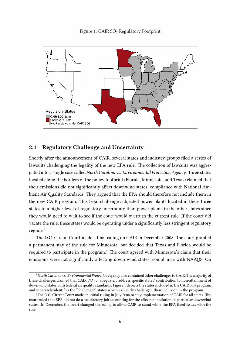
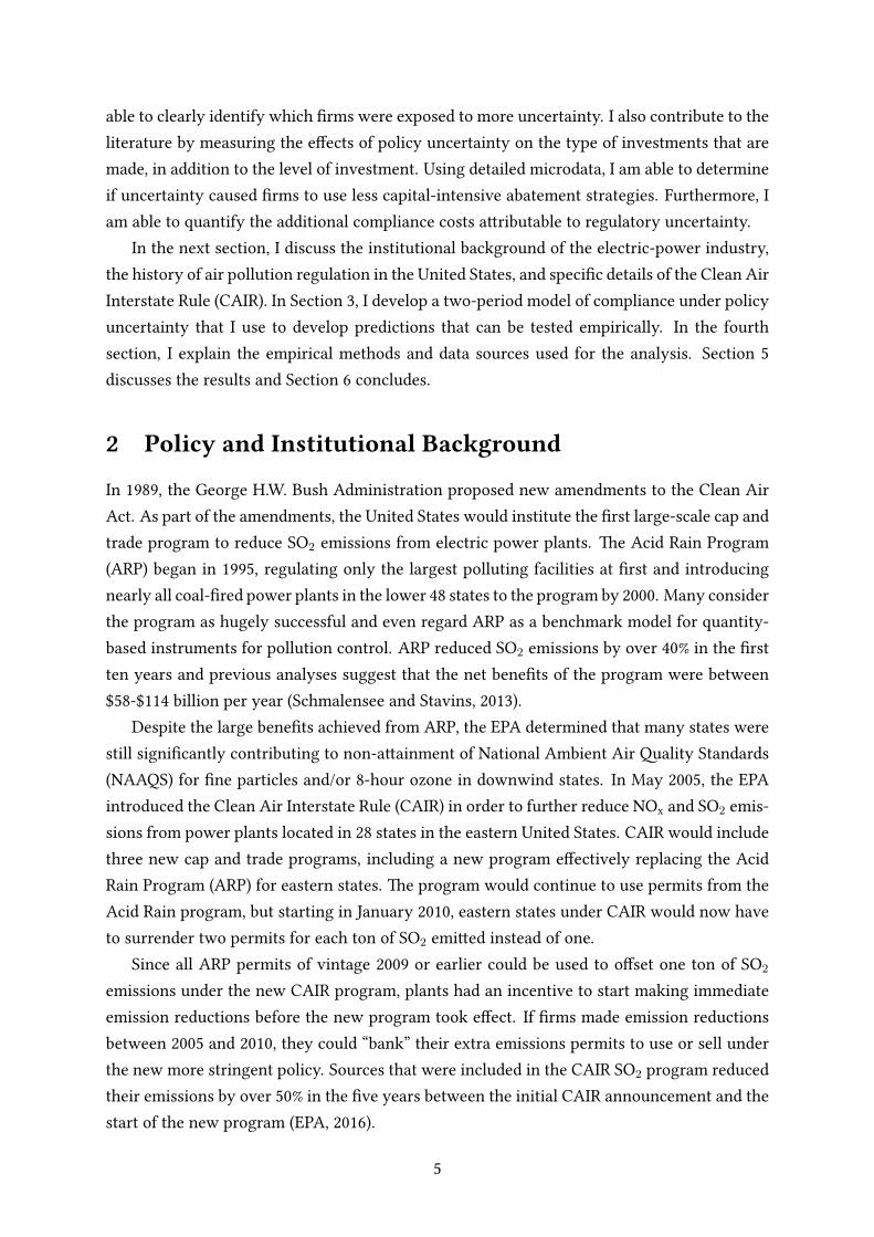
Figure 1: CAIR SO2 Regulatory Footprint

2.1 Regulatory Challenge and Uncertainty

Shortly a�er the announcement of CAIR, several states and industry groups �led a series of

lawsuits challenging the legality of the new EPA rule. �e collection of lawsuits was aggre-

gated into a single case calledNorth Carolina vs. Environmental Protection Agency. �ree states

located along the borders of the policy footprint (Florida, Minnesota, and Texas) claimed that

their emissions did not signi�cantly a�ect downwind states’ compliance with National Am-

bient Air �ality Standards. �ey argued that the EPA should therefore not include them in

the new CAIR program. �is legal challenge subjected power plants located in these three

states to a higher level of regulatory uncertainty than power plants in the other states since

they would need to wait to see if the court would overturn the current rule. If the court did

vacate the rule, these states would be operating under a signi�cantly less stringent regulatory

regime.8

�e D.C. Circuit Court made a �nal ruling on CAIR in December 2008. �e court granted

a permanent stay of the rule for Minnesota, but decided that Texas and Florida would be

required to participate in the program.9

�e court agreed with Minnesota’s claim that their

emissions were not signi�cantly a�ecting down wind states’ compliance with NAAQS. On

8North Carolina vs. Environmental ProtectionAgency also contained other challenges to CAIR. �e majority of

these challenges claimed that CAIR did not adequately address speci�c states’ contribution to non-a�ainment of

downwind states with federal air quality standards. Figure 1 depicts the states included in the CAIR SO2 program

and separately identi�es the “challenger” states which explicitly challenged their inclusion in the program.

9�e D.C. Circuit Court made an initial ruling in July 2008 to stay implementation of CAIR for all states. �e

court ruled that EPA did not do a satisfactory job accounting for the e�ects of pollution in particular downwind

states. In December, the court changed the ruling to allow CAIR to stand while the EPA �xed issues with the

rule.

6

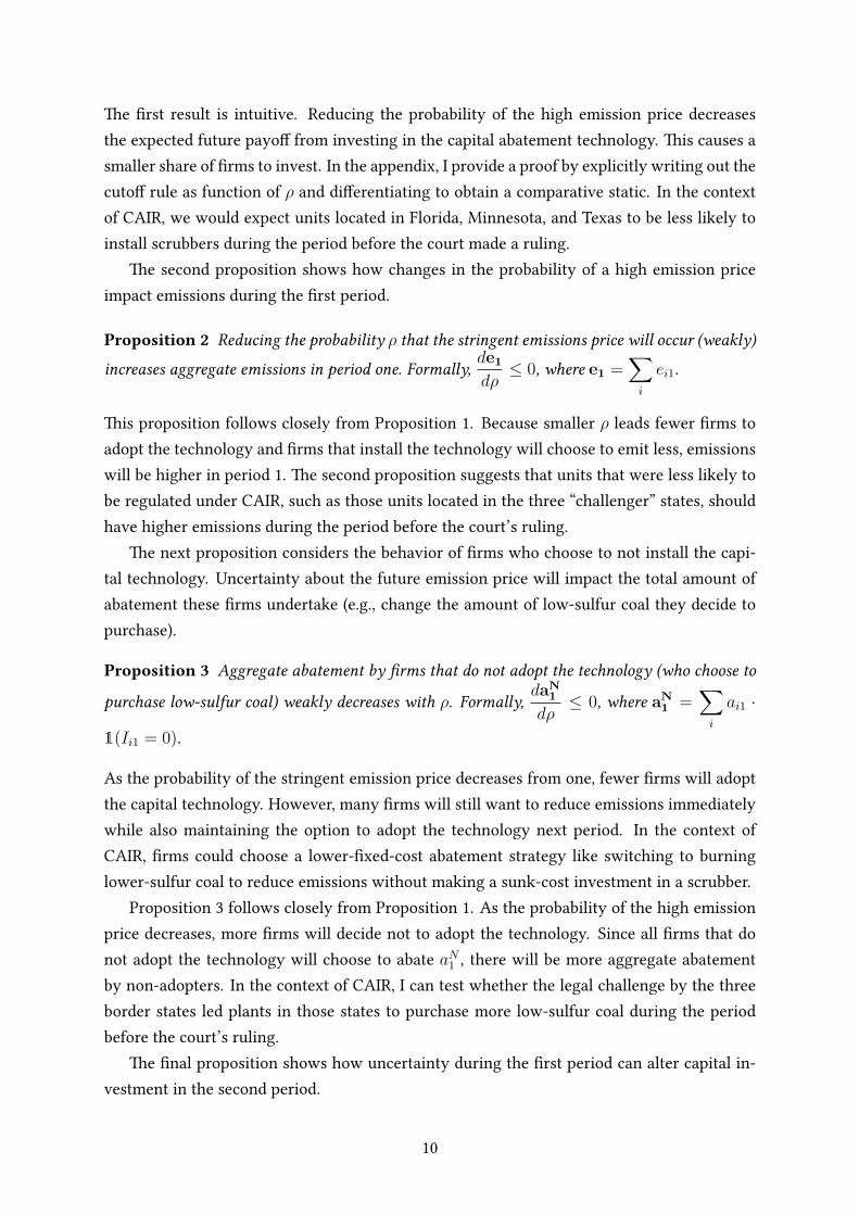
Figure 2: CAIR Regulatory Timeline

the other hand, the court rejected Texas and Florida’s similar claims.10

In 2010, the CAIR

SO2 program took e�ect for all of the initially planned states except for Minnesota. Figure 2

includes a timeline of important events in the rollout of CAIR.

�roughout the rest of the article, I focus on measuring the e�ects of regulatory uncer-

tainty that arose from the legal challenge to the CAIR program. �e legal challenge exposed

plants to varying levels of uncertainty. I exploit this variation to identify the e�ects of policy

uncertainty on pollution abatement, investment in control technologies, and coal purchases.

In the next section, I develop a two-period model of �rm compliance with a pollution regu-

lation. I use the model to establish testable predictions about �rm behavior under uncertainty.

I then test the theoretical predictions using unit-level data in the following sections.

3 Model of Compliance Under Policy Uncertainty

Consider a two-period model. In each period, �rms must pay a fee for each unit they emit.

In the �rst period, the regulator sets the emission price equal to P1. �e emission price could

also arise indirectly through an emission cap set by the regulator. However, the second-period

emission price is not revealed until a�er the �rst period is completed. With probability ρ ∈[0, 1], the regulator will impose a more stringent price PH

2 (more stringent emissions cap) and

with probability 1−ρ, she will impose a less stringent price PL2 (less stringent emissions cap),

where PH2 > PL

2 . �is uncertainty could result from a pending judicial review or from an

upcoming election.

�ere are M risk-neutral �rms and every �rm emits pollution as a byproduct of each

unit of output. For the case of an emission tax, M can be arbitrarily large. For an emission

cap, assume that M represents a small subset of �rms in the permit market such that each

�rm’s abatement and investment has no in�uence on the equilibrium permit price.11

Reducing

10For a more detailed discussion of the judicial challenge, please see Appendix A.

11For the empirical application, I focus on uncertainty that a�ected a small group of �rms and was unlikely

to have a substantial e�ect on the overall permit market.

7

emissions is costly for �rms. However, �rms can reduce their marginal abatement cost by

investing in a capital-intensive technology (i.e., a scrubber for removing SO2 emissions). Firms

that invest in the technology must incur a �xed cost Ki. �e cost of capital varies for each

�rm. In particular, capital costs are drawn from Ki ∼ F (K), where F is the cumulative

distribution function of K . I assume F (K) is continuous and di�erentiable. Investing in the

technology is irreversible. Firms can reduce their pollution without installing the capital-

intensive technology, but they must incur higher marginal abatement costs (e.g., switching to

low-sulfur coal).12

Absent any emission reductions, each �rm would emit e units of pollution. A �rm’s re-

alized emissions in period t (eit) are equal to the baseline emissions level net of abatement

ait, so eit = e− ait. Abatement cost C(ait, Iit) is a function of the level of abatement ait and

Iit ∈ {0, 1}, an indicator function that is equal to one if the �rm has installed the capital tech-

nology and zero otherwise. In particular,Ca(ait, 1) ≤ Ca(ait, 0) for all ait, where the subscript

a signi�es partial derivative with respect to ait. �is means the marginal cost of abatement

is lower once the capital technology is installed.13

Additionally, assume that the abatement

cost function is strictly increasing and convex in the level of abatement: Ca(ait, Iit) > 0 and

Caa(ait, Iit) > 0. Finally, normalize C(0, Iit) = 0. �is normalization implies that choosing

zero abatement is costless regardless of the technology decision.

Each period, �rms choose whether to install the technology at time t. �e installation de-

cision is permanent: if installed, the technology will remain in any future periods. In addition,

�rms choose ait and an output quantity qit to maximize expected pro�ts. For this analysis, I

assume that output quantity is �xed at q = q. �is is a reasonable assumption for coal-�red

power plants during the time period of this study since coal plants were almost always infra-

marginal and were already operating at a capacity constraint. �is assumption is also common

in literature (Fowlie, 2010) and allows the �rm’s abatement decision to be modeled indepen-

dently of the output decision. Omi�ing the �rm subscript i and superscript i for readability,

the �rm’s problem can be wri�en as:

min

a1,I1P1 · (e− a1) + C(a1, I1) +K · I1

+ 11+r

E[min

a2,I2{P2 · (e− a2) + C(a2, I2) +K · (I2 − I1)}

]s.t. at ∈ [0, e], It ∈ {0, 1}, I2 ≥ I1,

(1)

where E is the expectation operator taken over the uncertain emission price in period 2 and r

is the �rm’s per-period discount rate. �e �rm’s problem is to choose capital investment and

12In practice, switching to low-sulfur coal does incur a �xed cost to retro�t boilers and equipment; however,

these costs are generally very small in comparison to the capital cost of installing a scrubber.

13Modeling a new investment as reducing marginal abatement cost is standard in the theoretical literature

investigating environmental policy instruments and technology adoption, see Jung et al. (1996); Milliman and

Prince (1989); Requate and Unold (2003), and see Amir et al. (2008) for a discussion. �is assumption is consistent

with SO2 compliance costs at coal plants, because the marginal costs of running a scrubber a�er installation are

very low.

8

abatement to minimize the sum of current costs and expected costs in the next period, subject

to the constraint that abatement must be weakly greater than zero and less than the base-

line emissions level. �e �rm must also consider the irreversibility of the capital-investment

decision.

�e �rm’s optimal level of �rst-period abatement is determined by the following �rst order

condition for an interior solution:

Ca(a1, I1) = P1 (2)

�is �rst order condition is consistent with the standard intuition that �rms should set their

marginal cost of abatement equal to the equilibrium permit price. All �rms that do not install

the technology will choose the same abatement level aN1 , and all �rms that do install the

technology will choose aI1. Furthermore, it must be true that aN1 ≤ aI1, which follows from

the assumption that Ca(at, 1) ≤ Ca(at, 0) for all at.

�e capital investment choice is a dynamic decision. A pro�t-maximizing �rm must con-

sider not only the direct costs and bene�ts of investing today but also the opportunity cost

of waiting until next period to decide a�er the uncertainty has been resolved. �e solution

to the problem will consist of a cuto� rule for investment; all �rms with a capital investment

cost Ki ≤ K∗1 will install the technology, and all �rms with higher capital costs will not.14

A �rm should install the capital technology in the �rst period if the expected net costs from

installing immediately are less than the expected costs from waiting until the second period

to decide. In particular, �rms should invest if:

P1 · (e− aI1) + C(aI1, 1) +K + E[min

a2{P2 · (e− a2) + C(a2, 1)}]

≤ P1 · (e− aN1 ) + C(aN1 , 0) + E[min

a2,I2{P2 · (e− a2) + C(a2, I2) +K · I2}]

(3)

We now consider the testable predictions regarding �rm behavior implied by the model.

Proofs of all the propositions are provided in the appendix.

3.1 �eoretical Predictions

�e �rst proposition considers how a change in the probability of the more stringent policy

(ρ) a�ects �rms’ decision to invest in the capital technology in the �rst period.

Proposition 1 Reducing the probability ρ that the stringent emission price will occur will reduceinvestment in the capital technology in the �rst period. Formally, F (K∗1) (weakly) increases inρ.

14See Requate and Unold (2003) for more details.

9

�e �rst result is intuitive. Reducing the probability of the high emission price decreases

the expected future payo� from investing in the capital abatement technology. �is causes a

smaller share of �rms to invest. In the appendix, I provide a proof by explicitly writing out the

cuto� rule as function of ρ and di�erentiating to obtain a comparative static. In the context

of CAIR, we would expect units located in Florida, Minnesota, and Texas to be less likely to

install scrubbers during the period before the court made a ruling.

�e second proposition shows how changes in the probability of a high emission price

impact emissions during the �rst period.

Proposition 2 Reducing the probability ρ that the stringent emissions price will occur (weakly)

increases aggregate emissions in period one. Formally,de1dρ≤ 0, where e1 =

∑i

ei1.

�is proposition follows closely from Proposition 1. Because smaller ρ leads fewer �rms to

adopt the technology and �rms that install the technology will choose to emit less, emissions

will be higher in period 1. �e second proposition suggests that units that were less likely to

be regulated under CAIR, such as those units located in the three “challenger” states, should

have higher emissions during the period before the court’s ruling.

�e next proposition considers the behavior of �rms who choose to not install the capi-

tal technology. Uncertainty about the future emission price will impact the total amount of

abatement these �rms undertake (e.g., change the amount of low-sulfur coal they decide to

purchase).

Proposition 3 Aggregate abatement by �rms that do not adopt the technology (who choose to

purchase low-sulfur coal) weakly decreases with ρ. Formally,daN

1

dρ≤ 0, where aN

1 =∑i

ai1 ·

1(Ii1 = 0).

As the probability of the stringent emission price decreases from one, fewer �rms will adopt

the capital technology. However, many �rms will still want to reduce emissions immediately

while also maintaining the option to adopt the technology next period. In the context of

CAIR, �rms could choose a lower-�xed-cost abatement strategy like switching to burning

lower-sulfur coal to reduce emissions without making a sunk-cost investment in a scrubber.

Proposition 3 follows closely from Proposition 1. As the probability of the high emission

price decreases, more �rms will decide not to adopt the technology. Since all �rms that do

not adopt the technology will choose to abate aN1 , there will be more aggregate abatement

by non-adopters. In the context of CAIR, I can test whether the legal challenge by the three

border states led plants in those states to purchase more low-sulfur coal during the period

before the court’s ruling.

�e �nal proposition shows how uncertainty during the �rst period can alter capital in-

vestment in the second period.

10

Proposition 4 Reducing the probability ρ that the stringent emission price will occur will causemore capital investment in the second period if the stringent emission price happens to be realized.

As ρ decreases, fewer �rms will adopt the technology in period 1. In the case that the high

emission price PH2 does occur, a larger share of �rms will then choose to adopt in the second

period. �is proposition suggests that a�er the court ruled to include Texas and Florida in

CAIR, we should see relatively more scrubbers installed in those states than in other CAIR-

regulated states a�er the court decision.

Table 1: �eoretical Predictions and Associated Empirical Predictions

�eoretical Prediction Empirical Prediction Predicted Sign

Proposition 1 ρ ↓ ⇒∑

i Ii1 ↓

Units in “challenger”

states should be less

likely to install a

scrubber.� ∗

β1 < 0

Proposition 2 ρ ↓ ⇒ e1 ↑Units in “challenger”

states should have

higher emissions.� ∗

β1 > 0

Proposition 3 ρ ↓ ⇒ aN1 ↑

Plants in “challenger”

states should decrease

the sulfur content of

their coal purchases.� ∗

β1 < 0

Proposition 4 If P2 = PH2 , then ρ ↓

⇒∑

i Ii2 ↑

Units in “challenger”

states should be more

likely to install a

scrubber a�er the

court ruled to enforce

the high emission

price.∗

βt > 0, ∀ t > 2009

�Before the court ruling.

∗Relative to other units regulated under CAIR.

Testing Proposition 2 is the central focus of the empirical section of this paper. In partic-

ular, I test if reductions in the probability of regulation increased emissions during the period

of uncertainty. �e judicial challenge of CAIR by three states generated variation in �rms’

probability of having to comply with CAIR. Speci�cally, plants in these three states were less

likely to have to comply with the new regulation than �rms in other states under CAIR. I

use this variation to test for di�erences in emission reductions, and also to directly test for

di�erences in investment and abatement methods (Propositions 1 and 3). Furthermore, I test

whether investment in scrubbers (capital technology) increased more in these states a�er the

court ruled that they would need to comply (Proposition 4).

Table 1 summarizes the propositions. Column 2 provides a short description of the theo-

retical result and the third column describes the associated empirical prediction that can be

11

taken to the data. �e fourth column provides the theoretically predicted regression coe�-

cients, which are discussed in detail in the following sections.

4 Data and Empirical Methods

In order to test the propositions from the previous section, I collect source-level data from the

EPA’s Continuous Emissions Monitoring System (CEMS) for the years 2002-2011.15

CEMS is

a nation-wide database used to monitor compliance with federal emissions programs such as

the Acid Rain Program and the Clean Air Interstate Rule SO2 Trading Program.

�e EPA Clean Air Markets Program database allows users to collect source-level emis-

sions data at the hourly level. For this study, I aggregate the data to the annual level. �e

CEMS data include gross output (MWH), NOx emissions (tons), CO2 emissions (tons), SO2

emissions (tons), and heat input (MMBtu) at the boiler level. I am interested in reductions

in SO2 emissions so I restrict the sample to only coal-�red boilers.16

�e CEMS database in-

cludes all generators with nameplate capacity over 25 MW and thus includes essentially all

coal units in the contiguous United States. �e EPA also provides descriptive data for each

unit including the capacity, geographic coordinates, beginning date of operation, name of

operating company, and a description of any pollution control technology installed.

To be�er understand how uncertainty a�ects coal-purchasing decisions, I also obtain plant

level fuel receipts data from the Energy Information Agency (EIA) and the Federal Energy

Regulatory Commission (FERC). From 2002-2007, plants that were subject to cost-of-service

regulation reported fuel purchases annually on FERC Form 423, and deregulated plants re-

ported on EIA Form 423. From 2007-2011, all coal plants reported fuel purchases on a single

form, EIA Form 923. �e fuel receipts data include the quantity of coal purchased (short tons),

sulfur content of fuels (percentage of weight), heat content (MMBtu), and ash content. Price

and other fuel contract details are provided for regulated plants. A useful feature of the fuel

receipts data is that it indicates if a plant is under cost-of-service regulation. I merge the EIA

data with the EPA data using unique Plant ID numbers included in both data sets. �is allows

me to identify the regulatory status of each unit in the EPA data.

Table 2 provides summary statistics for units located in each of the three groups of states

in 2004, right before CAIR was announced. �e �rst column includes all units included in the

CAIR SO2 trading program except the three “challenger” states. �e third column summarizes

units located in Florida, Minnesota, and Texas and the second column includes all other coal

units. Units in CAIR had higher emission rates on average than non-CAIR units and units in

the three “challenger” states. Units in CAIR also were older than other units, less likely to be

regulated, less likely to have a scrubber installed, and produced less gross output. Distance to

152002-2011 is the time frame for the main analysis. I also collect data going back as far 1996 that is used for

an additional test.

16Coal boilers emit over 99.5% of all SO2 emissions from the electric-power industry.

12

Table 2: Coal Unit Summary Statistics by Group Before CAIR

CAIR Non-CAIR Challenger Total

Gross Load (TWH) 1.956 2.583 3.162 2.194

(1.847) (1.792) (1.917) (1.881)

Distance to PRB (Miles) 1904.9 991.7 1747.1 1701.2

(389.2) (593.0) (627.5) (589.8)

Regulated (0,1) 0.723 0.915 0.778 0.768

(0.448) (0.279) (0.418) (0.422)

Age (Years) 39.91 31.85 26.68 37.06

(10.79) (10.28) (11.83) (11.71)

Capacity (Max HI bil. btu) 3.491 4.301 5.232 3.815

(2.764) (3.053) (3.197) (2.916)

Scrubber (0,1) 0.152 0.418 0.395 0.229

(0.359) (0.495) (0.492) (0.420)

SO2 2004 (lbs/MMBtu) 1.406 0.574 0.705 1.171

(0.948) (0.507) (0.437) (0.914)

SO2 2009 (lbs/MMBtu) 1.077 0.532 0.625 0.923

(0.891) (0.489) (0.413) (0.824)

SO2 Di�erence (lbs/MMBtu) -0.329 -0.0420 -0.0801 -0.248

(0.696) (0.234) (0.264) (0.611)

N 880 200 88 1,168

�e descriptive statistics describe boiler characteristics in 2004. Distance to PRB is the unit’s distance to the

Powder River Coal Basin in Wyoming, this serves a proxy for the unit’s ability to purchase lower-sulfur subbi-

tuminous coal. Capacity is measured as the unit’s maximum heat input in btu (billions). “SO2 Di�erence” is the

change in emission rates between 2004 and 2009. Standard deviations are in parentheses.

PRB is the unit’s distance to the Powder River Coal Basin in Wyoming. Units in Non-CAIR

states were much closer to the Powder River Basin on average and likely had greater access

to low-sulfur coal.

Comparing the 2004 SO2 emission rates in the bo�om of Table 2 to the emission rates for

2009, it’s clear that emission reductions were much larger in CAIR states. �e average emis-

sion rate dropped by 0.33 lbs. per MMBtu in CAIR states, while it only dropped by 0.04 lbs.

per MMBtu in non-CAIR states and 0.08 lbs. per MMBtu in “challenger” states. CAIR states

were also more likely to install scrubbers between 2004 and 2009. �ese descriptive results

are consistent with the theory that regulatory uncertainty delays abatement and investment,

but on their own are not proof of a causal relationship. It is possible the di�erence between

emission reductions in “challenger” states and other CAIR states were driven by di�erences

13

in unit characteristics between the two groups and not by regulatory uncertainty. Another

possibility is selection into the “challenger” group was itself endogenous. �is would be the

case if generation companies located in Florida, Minnesota, and Texas had a particular prefer-

ence against reducing emissions and decided to �le the lawsuit for that reason. An additional

possibility is that emission rates in each of these groups were already following di�erent time

trends not associated with CAIR at all. In the next discussion, I describe the empirical model

used to address these potential concerns.

4.1 Empirical Model and Identi�cation

In this section, I discuss the econometric model used to test the predictions from the theoretical

model. First, I describe the di�erence-in-di�erences (DID) approach used to test if the legal

challenge of CAIR caused a decrease in pollution abatement (Proposition 2). I then describe

how an analogous empirical approach can be used to test Proposition 3. Speci�cally, I test

if uncertainty generated by the legal challenge caused �rms that didn’t invest in scrubbers

to increase purchases of low-sulfur coal. Next, I explain how a slightly modi�ed but simple

framework can be used to test whether the legal challenge reduced investment in capital-

intensive pollution controls (scrubbers) during the period before the uncertainty was resolved

(Proposition 1). Finally, I introduce a regression framework to test if relative investment in

scrubbers changed a�er the court ruling (Proposition 4).

4.1.1 Empirical Test of Proposition 2

In order to test Proposition 2, I compare changes in SO2 emission rates a�er the policy an-

nouncement at units subject to additional legal uncertainty to other units in CAIR and to units

not regulated by CAIR. I use both regression and matching approaches to control for observ-

able characteristics of the coal units. �e states never regulated under CAIR serve as a natural

“control” group. All states initially intended to be regulated under CAIR are de�ned as the

“treatment” group. Additionally, I de�ne a “treatment” subgroup composed of units located

in one of the states subjected to additional regulatory uncertainty.

A DID approach relaxes the assumption that the average level of the dependent variable

would have been the same absent “treatment”. Instead, it must be true that trends in the

dependent variable would have been the same absent “treatment”. By adding controls, we are

ensured that the estimated e�ect is only being identi�ed o� of units with similar observable

characteristics. I start by estimating the following regression:

Yit = β11[Challenger]it + β21[CAIR]it + x′iγ + γt + εit (4)

14

�e dependent variable is unit i′s SO2 emission rate in lbs. per MMBtu17

in year t. 1[Challengerit]

is an indicator variable, equal to one if the year is 2005-2009 and the unit is located in a Min-

nesota, Florida, or Texas. �e period of 2005-2009 includes years a�er the policy was an-

nounced, but before the court made its ruling. 1[CAIRit] is an indicator variable, set equal to

one if the unit is located in a CAIR state including Florida, Minnesota, and Texas, and the year

is 2005-2009. γt is a set of year �xed e�ects and x′i contains unit �xed e�ects in my preferred

speci�cation. For speci�cations without unit �xed e�ects, x′i contains a vector of controls

such as the unit’s age, regulatory status, distance to the Powder River Basin, and emission

rate in 2004 before the policy was announced. Several studies have shown compliance choice

can be a�ected by a plant’s regulatory status (Cicala (2015), Fowlie (2010)), this control en-

sures only di�erences between plants under the same regulatory regime are being compared.

I also control for the unit’s distance to the Powder River Basin, the Powder River Basin is the

primary mining location for low-sulfur coal, so this variable proxies for a �rm’s ability to pur-

chase low-sulfur coal. Finally, I control for each unit’s emission rate in 2004, since abatement

opportunities may be limited if a unit already has a very low emission rate.

�e coe�cient of interest is β1. I include units in Florida, Minnesota, and Texas in both

the “CAIR” and “Challenger” groups. �erefore, β1 can be interpreted as the average change

in emission rates in Florida, Minnesota, and Texas relative to units in other CAIR-regulated

states. Proposition 2 predicts that units in the “challenger” states should be less likely to

reduce emissions. If this is true, β1 should be positive. On the other hand, we would expect β2

to be negative because units in states regulated under CAIR should be more likely to reduce

emissions relative to units in states that are not subject to the rule.

An important identifying assumption is unconfoundedness; it must be true that a�er con-

trolling for observed covariates (unit �xed e�ects), average emission rates for the treatment

groups and the control group would have followed parallel trends absent the intervention.

Figure 3 shows the average SO2 emissions trends for each of the three groups in the years

before the CAIR SO2 program was announced in 2005. A visual inspection shows no system-

atic deviation in the slopes of the trend lines between the groups. Furthermore, the trends had

been nearly �at for each of the groups during the four years before the policy was announced.

�ere is a decrease in emission rates for each of the groups at the end of the 1990s. �is de-

crease was the result of compliance with Phase 2 of the Acid Rain Program. As an indirect

test of the unconfoundedness assumption, I estimate the DID model (4) with the pre-period as

1996-1999, and the post-period as 2000-2001. �e results of these regressions can be found in

Panel A of Table 8 of the appendix. In all speci�cations, I fail to reject the null hypothesis that

β1 = 0. �e point estimates are also small in magnitude. Panel B of Table 8 of the appendix

presents regressions with the dependent variable as a binary choice to install a scrubber. I

17I use SO2 per MMBtu instead of SO2 per MWH because gross output data is missing for some units in the

sample. As a robustness check I also run the model with SO2 per MWH and annual SO2 emissions (tons) as the

outcome variable.

15

Figure 3: SO2 Emission Rates Trends by Group

�e plo�ed trend lines represent the mean SO2 emission rate (residual) for each

group a�er controlling for unit �xed e�ects. �e �rst red vertical line indicates the

initial announcement of CAIR. �e second vertical red line represents the date the

court made its �nal ruling.

also fail to reject the null hypothesis that units in Texas, Florida, and Minnesota were equally

likely to install scrubbers to comply with the Acid Rain Program Phase 2 relative to other

CAIR states. �is exercise provides evidence that units in Texas, Florida, and Minnesota were

not systematically di�erent from units in other CAIR states when complying with previous

SO2 regulations.

Even if compliance decisions in “challenger” states were not di�erent in the past, it is still

possible �rm ownership has changed over time and utility executives located in these states

now have a stronger preference against making emission reductions. To account for potential

bias through this channel, I also run the model (4) on a restricted sample only including oper-

ating companies that owned plants in “challenger” states and also in other CAIR states. I also

include operator �xed e�ects. �is speci�cation ensures I am comparing abatement choices

in states subject to more regulatory uncertainty to abatement choices in other states, while

holding managerial preferences constant.

Finally, to ensure that the regression estimates are unbiased, the stable unit treatment

value assumption (SUTVA) must hold. �is means that regulatory uncertainty in Texas,

Florida, and Minnesota must not have changed the abatement choices of units outside of those

states. �is assumption may not hold if power plants in the “challenger” states made up a large

enough portion of the SO2 permit market to signi�cantly a�ect allowance prices. �ere are

two reasons why a violation of SUTVA is unlikely to cause problems for identifying a causal

e�ect. First, since emissions from power plants in the three “challenger” states made up only

16

8.9% of total SO2 emissions in 2004, the exclusion of these three states would have decreased

permit demand by 4.8%.18

�is change would be unlikely to cause a large enough decrease

in permit prices to drastically change abatement decisions in other states. Secondly, even if

the legal challenge by Texas, Minnesota, and Florida had an e�ect on permit prices, the e�ect

would likely bias against �nding β1 > 0. Since the legal challenge reduced the probability

that �rms in the “challenger” states would have to comply with CAIR, this would reduce ex-

pected demand for permits and tend to drive down permit prices. Lower permit prices should

cause other �rms in CAIR to be less likely to make early investments in pollution control.

Furthermore, increased uncertainty about future permit prices should cause other plants reg-

ulated under CAIR to be more likely to delay their own investment. �is would bias against

�nding the result that plants in “challenger” states were more likely to delay making pollution

reductions relative to other CAIR-regulated plants.

4.1.2 Empirical Test of Proposition 1 and 3

In addition to measuring the impact of regulatory uncertainty on pollution outcomes, I am

also interested in the mechanisms driving any di�erences in pollution. Coal units typically

have two options for reducing SO2 emissions. Units can install a �ue-gas desulfurization

system (scrubber) or they can switch to lower-sulfur coal. Installing a scrubber requires a

relatively large �xed-cost investment and has low operating costs. In contrast, switching coal

rank typically requires a relatively smaller �xed cost and higher variable costs. �e theoret-

ical model predicts that coal units that were subjected to additional legal uncertainty should

increase total purchases of low-sulfur coal (low �xed-cost abatement). For example, we may

see �rms in the “challenger” states making more non-scrubber abatement than �rms in states

where the probability of regulation was closer to one. I estimate the direction and magnitude

of this e�ect by running the same DID regression with sulfur content of coal purchases as

the dependent variable. Since coal purchase data is recorded at the plant level, I run these

regressions with observations at the plant-year level instead of the boiler-year level. If β1 is

negative, it would provide evidence that plants located in the states challenging the ruling

were more likely to reduce the sulfur content of their coal during the period of uncertainty.

I can also use a similar framework to test if units with a lower probability of being regulated

under CAIR were less likely to install scrubbers during the period of uncertainty (Proposition

1). To test the �rst proposition, it does not make sense to estimate a DID model with a binary

irreversible decision as the outcome. Instead, I restrict the sample to only units that did not

already have a scrubber installed in 2004. I then estimate both linear probability and probit

models where the dependent variable is a binary variable, set equal to one if the unit installed

a scrubber by 2009, and set equal to zero otherwise.

18Total demand for permits can be determined by multiplying 2004 SO2 emissions by 2 for units included in

CAIR, and multiplying 2004 SO2 emissions by 1 for non-CAIR units and summing across all units.

17

4.1.3 Empirical Test of Proposition 4

�e fourth result from the analytic model predicts that we should see a relative increase in

scrubber investment at plants in Florida and Texas a�er the court ruled to enforce CAIR. To

test whether the relative probability that scrubbers were installed changed a�er the court’s

decision, I estimate the following model:

1[Scrubber]it = βt1[Challenger]it · 1[year]t + λt1[CAIR]it · 1[year]t + x′iγ + γt + εit,

(5)

where1[Scrubberit] is an indicator variable, set equal to one if unit i has a scrubber installed in

year t and zero otherwise, and1[year]t is a year dummy. Again, x′i controls for unit observable

characteristics and also contains a dummy for if the unit had a scrubber installed during year

t − 1. Conditional on not already having installed a scrubber, βt is the average additional

probability that units in “challenger” states in year t install a scrubber, relative to units in the

other “CAIR” states.

In order to examine outcomes a�er the court made the decision to include Florida and

Texas in CAIR, I expand the sample to include the years 2010 and 2011.19

I also drop units

in Minnesota since I want to test if the probability of installing a scrubber went up a�er the

court ruled that the two states would have to comply.20

Finding βt is negative for years before

the court decision, and βt is positive a�er the court decision, would support the theoretical

prediction that units that faced a lower probability of being regulated should be less likely to

invest in pollution controls in the period before the court decision but should be relatively

more likely to install a scrubber in the years following the decision.

4.2 Alternative Estimators

A potential weakness of the DID estimator with a vector of linear controls is it implicitly

assumes the treatment e�ect must be homogeneous. �is assumption would be violated if

abatement choices are di�erent on average at plants with di�erent characteristics. Previous

work by Cicala (2015) and Fowlie (2010) show plants operating under cost-of-service regu-

lation have been more likely to install capital-intensive technologies. �ere is also reason to

believe pollution controls are less likely to be installed on older units closer to retirement.

To relax the assumption of homogeneous treatment e�ects, I estimate a semi-parametric

di�erence-in-di�erences estimator in the spirit of Abadie (2005). �is estimator has two main

steps. First, I �exibly estimate a propensity score function. Secondly, I reweight the observa-

19In 2011, the EPA announced a replacement policy for CAIR called the Cross State Air Pollution Rule

(CSAPR), for that reason I do not consider any data beyond 2011 because any abatement choices beyond that

point are likely related to the new policy.

20I also investigate abatement and investment trends for each state individually in the appendix. �ere were

only 9 units without scrubbers in MN a�er the court ruling and none installed scrubbers in 2010-2011.

18

tions in the treatment and control groups using the estimated propensity scores.

More formally, let Y 0(i, t) represent the emission rate unit i would a�ain at time t in

absence of treatment. Similarly, let Y 1(i, t) represent the emission rate unit i would a�ain

at time t if exposed to the treatment. �e e�ect of the treatment on the outcome for unit

i at time t is de�ned as Y 1(i, t) − Y 0(i, t). Additionally, let D(i) be an indicator function

determining if unit i receives the treatment. Also de�ne P (D = 1|X) as the propensity score,

the probability a unit receives treatment conditional on observed covariates. For this analysis,

the treatment group will be all units located in the “challenger” states and the control group

will be all other units in CAIR.21

I use the year 2004 emission rate as the pre-period observation

and the 2009 emission rate as the post-period observation. �e objective is to estimate the

average treatment e�ect on the treated group (ATT): E[Y 1(i, 2009)− Y 0(i, 2004)|D(i) = 1].

Estimation of the ATT requires a weaker assumption on distribution of covariates than would

be required to estimate the population average treatment e�ect (ATE). For identi�cation, I

require P (D = 1|X) < 1, in addition to the unconfoundedness assumption.22

�is overlap

condition is satis�ed for the observed covariates.23

�e average treatment on the treated is

given by:

ATT = E[Y 1(i, 2009)− Y 0(i, 2009)|D(i) = 1]

=

∫E[Y 1(i, 2009)− Y 0(i, 2009)|X(i), D(i) = 1]dP (D = 1|X)

=

∫E[ρo · (Y (i, 2009)− Y (i, 2004))|X(i)]dP (D = 1|X)

= E[ρ0 · (Y (i, 2009)− Y (i, 2004)) · P (D = 1|X)

P (D = 1)

]= E

[(Y (i, 2009)− Y (i, 2004))

P (D = 1)· D − P (D = 1|X)

(1− P (D = 1|X))

]

where ρ0 = D−P (D=1|X)P (D=1|X)(1−P (D=1|X))

(6)

�e third line follows from the unconfoundedness assumption, a�er controlling for observed

covariates, the treatment and control groups would have followed parallel paths absent the

intervention. �e estimator is the sample analog of the ��h line in (6). Intuitively, the estima-

tor is down weighting the distribution of Y (i, 2009)− Y (i, 2004) for the untreated group for

values of the covariates which are over-represented among the untreated and weighting-up

Y (i, 2009) − Y (i, 2004) for those values of the covariates under-represented among the un-

treated. I estimate the propensity score using a �exible logit model that includes interactions

of all the covariates and quadratic terms.

In addition to the propensity-score-weighted estimator, I also implement a nearest-neighbor-

21�e semi-parametric DID estimator only allows for one treatment group and one control group so I omit

units outside CAIR.

22Estimation of the ATE requires the overlap condition: 0 < P (D = 1|X) < 1.

23�e data appendix includes marginal kernel density plots of the continuous covariates for each group.

19

matching estimator (Abadie and Imbens, 2006). I force units to be matched exactly on the

binary “Regulated” variable and then I choose nearest-neighbor matches using Mahalanobis

distance metric over the three continuous variables.24

I also use the Abadie and Imbens (2006)

bias correction to adjust for inexact matches in the control group. �e nearest-neighbor esti-

mator is:

ATT =1

N1

∑i∈Υ1

{(Y (i, 2009)− Y (i, 2004)

)−∑k∈Υ0

wik(Y (k, 2009)− Y (k, 2004)

)}(7)

where Υ1 is the set of all units in the treatment group, N1 is the number of units in the

treatment group, and Υ0 includes all units in the control group. �e weight placed on unit k

when constructing the counterfactual estimate for treated facility i is wik.

5 Results

In this section, I present the primary empirical results and conduct a series of robustness

checks.

5.1 E�ects of Policy Uncertainty on Emissions (Prop. 2)

Table 3 presents regression results from equation 4. �e primary outcome of interest is SO2

emission rate in pounds per unit of heat input. �e last three columns include year �xed

e�ects, column (3) includes state �xed e�ects and column (4) includes unit �xed e�ects. In all

speci�cations, standard errors are clustered at the unit level.25

In each speci�cation, CAIR (β2) is negative and statistically signi�cant at the 1% level.

�is means units in states that were scheduled to be part of the CAIR SO2 program reduced

emissions more than units not scheduled to participate in the years before the program be-

gan, 2005-2009. Units anticipating the lower emissions cap under CAIR had an incentive to

make early emission reductions because they could bank current allowances to use and sell

under the new program. On the other hand, Challenger (β1) is positive and statistically

signi�cant at the 1% level in all speci�cations. �is provides evidence that units exposed to

increased regulatory uncertainty were less likely to reduce their emissions relative to other

states included in CAIR. �is is consistent with Proposition 2 from Section 3. Since there was

increased uncertainty as to whether units in these states would actually have to comply with

the new regulations, they had a higher option value to delay abatement that required sunk

irreversible investments. Additionally, I can compare emission reductions in the “challenger”

24�e continous variables include the unit’s distance to the Powder River Basin, boiler age, and baseline

emission rate in 2004.

25�e results are also robust to clustering at the plant level, operating-company level, state-year level, and

state level.

20

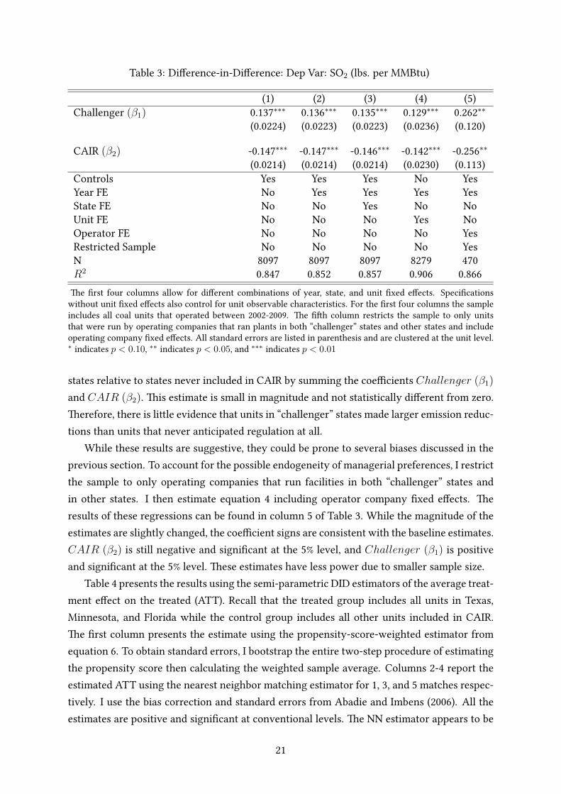
Table 3: Di�erence-in-Di�erence: Dep Var: SO2 (lbs. per MMBtu)

(1) (2) (3) (4) (5)

Challenger (β1) 0.137∗∗∗

0.136∗∗∗

0.135∗∗∗

0.129∗∗∗

0.262∗∗

(0.0224) (0.0223) (0.0223) (0.0236) (0.120)

CAIR (β2) -0.147∗∗∗

-0.147∗∗∗

-0.146∗∗∗

-0.142∗∗∗

-0.256∗∗

(0.0214) (0.0214) (0.0214) (0.0230) (0.113)

Controls Yes Yes Yes No Yes

Year FE No Yes Yes Yes Yes

State FE No No Yes No No

Unit FE No No No Yes No

Operator FE No No No No Yes

Restricted Sample No No No No Yes

N 8097 8097 8097 8279 470

R20.847 0.852 0.857 0.906 0.866

�e �rst four columns allow for di�erent combinations of year, state, and unit �xed e�ects. Speci�cations

without unit �xed e�ects also control for unit observable characteristics. For the �rst four columns the sample

includes all coal units that operated between 2002-2009. �e ��h column restricts the sample to only units

that were run by operating companies that ran plants in both “challenger” states and other states and include

operating company �xed e�ects. All standard errors are listed in parenthesis and are clustered at the unit level.

∗indicates p < 0.10,

∗∗indicates p < 0.05, and

∗∗∗indicates p < 0.01

states relative to states never included in CAIR by summing the coe�cients Challenger (β1)

and CAIR (β2). �is estimate is small in magnitude and not statistically di�erent from zero.

�erefore, there is li�le evidence that units in “challenger” states made larger emission reduc-

tions than units that never anticipated regulation at all.

While these results are suggestive, they could be prone to several biases discussed in the

previous section. To account for the possible endogeneity of managerial preferences, I restrict

the sample to only operating companies that run facilities in both “challenger” states and

in other states. I then estimate equation 4 including operator company �xed e�ects. �e

results of these regressions can be found in column 5 of Table 3. While the magnitude of the

estimates are slightly changed, the coe�cient signs are consistent with the baseline estimates.

CAIR (β2) is still negative and signi�cant at the 5% level, and Challenger (β1) is positive

and signi�cant at the 5% level. �ese estimates have less power due to smaller sample size.

Table 4 presents the results using the semi-parametric DID estimators of the average treat-

ment e�ect on the treated (ATT). Recall that the treated group includes all units in Texas,

Minnesota, and Florida while the control group includes all other units included in CAIR.

�e �rst column presents the estimate using the propensity-score-weighted estimator from

equation 6. To obtain standard errors, I bootstrap the entire two-step procedure of estimating

the propensity score then calculating the weighted sample average. Columns 2-4 report the

estimated ATT using the nearest neighbor matching estimator for 1, 3, and 5 matches respec-

tively. I use the bias correction and standard errors from Abadie and Imbens (2006). All the

estimates are positive and signi�cant at conventional levels. �e NN estimator appears to be

21

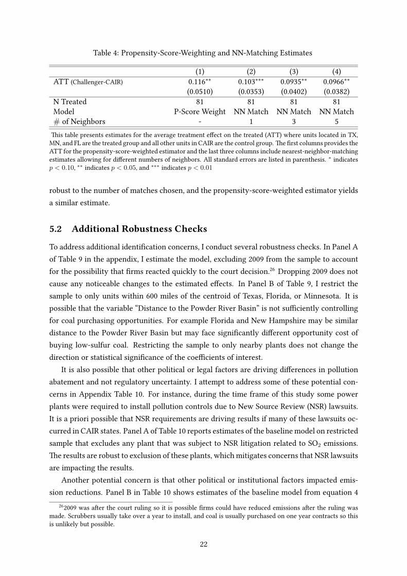
Table 4: Propensity-Score-Weighting and NN-Matching Estimates

(1) (2) (3) (4)

ATT (Challenger-CAIR) 0.116∗∗

0.103∗∗∗

0.0935∗∗

0.0966∗∗

(0.0510) (0.0353) (0.0402) (0.0382)

N Treated 81 81 81 81

Model P-Score Weight NN Match NN Match NN Match

# of Neighbors - 1 3 5

�is table presents estimates for the average treatment e�ect on the treated (ATT) where units located in TX,

MN, and FL are the treated group and all other units in CAIR are the control group. �e �rst columns provides the

ATT for the propensity-score-weighted estimator and the last three columns include nearest-neighbor-matching

estimates allowing for di�erent numbers of neighbors. All standard errors are listed in parenthesis.∗

indicates

p < 0.10,∗∗

indicates p < 0.05, and∗∗∗

indicates p < 0.01

robust to the number of matches chosen, and the propensity-score-weighted estimator yields

a similar estimate.

5.2 Additional Robustness Checks

To address additional identi�cation concerns, I conduct several robustness checks. In Panel A

of Table 9 in the appendix, I estimate the model, excluding 2009 from the sample to account

for the possibility that �rms reacted quickly to the court decision.26

Dropping 2009 does not

cause any noticeable changes to the estimated e�ects. In Panel B of Table 9, I restrict the

sample to only units within 600 miles of the centroid of Texas, Florida, or Minnesota. It is

possible that the variable “Distance to the Powder River Basin” is not su�ciently controlling

for coal purchasing opportunities. For example Florida and New Hampshire may be similar

distance to the Powder River Basin but may face signi�cantly di�erent opportunity cost of

buying low-sulfur coal. Restricting the sample to only nearby plants does not change the

direction or statistical signi�cance of the coe�cients of interest.

It is also possible that other political or legal factors are driving di�erences in pollution

abatement and not regulatory uncertainty. I a�empt to address some of these potential con-

cerns in Appendix Table 10. For instance, during the time frame of this study some power

plants were required to install pollution controls due to New Source Review (NSR) lawsuits.

It is a priori possible that NSR requirements are driving results if many of these lawsuits oc-

curred in CAIR states. Panel A of Table 10 reports estimates of the baseline model on restricted

sample that excludes any plant that was subject to NSR litigation related to SO2 emissions.

�e results are robust to exclusion of these plants, which mitigates concerns that NSR lawsuits

are impacting the results.

Another potential concern is that other political or institutional factors impacted emis-

sion reductions. Panel B in Table 10 shows estimates of the baseline model from equation 4

262009 was a�er the court ruling so it is possible �rms could have reduced emissions a�er the ruling was

made. Scrubbers usually take over a year to install, and coal is usually purchased on one year contracts so this

is unlikely but possible.

22

but only including units in states that had a Republican governor in 2006 and choose PUC

chairmen by appointment. In 2006, Texas, Minnesota, and Florida all had Republican gov-

ernors and appointed PUC chairmen. �is restricted sample a�empts to deal with possible

confounding political factors that would make installing pollution controls more feasible in

some states. Since most states did not have both a Republican governor and an appointed

PUC commission,27

75% of the observation are dropped. As a result, the estimated coe�cient

is no longer statistically signi�cant. However, the point estimate is still positive and of similar

magnitude. �is result suggests that the baseline result are not being driven by confounding

political factors.

I also account for the possibility that �rms were changing electricity output as a method

of compliance. In particular, I estimate the model with total annual SO2 emissions in tons as

the dependent variable. I also estimate the baseline DID regression with the natural logarithm

of SO2 in tons as the dependent variable and also with the natural logarithm of emission rate

as the outcome variable. �e results of all of these regressions are consistent with the baseline

model and are presented in Table 11 in the Appendix.

Finally, I present estimates with alternative standard error clusters. In Table 12, I allow

for clustering at the plant level, operating company level, and state level. �ese alternative

clusters do not change the signi�cance of the estimated e�ects.

5.3 Mechanisms (Props. 1 & 3)

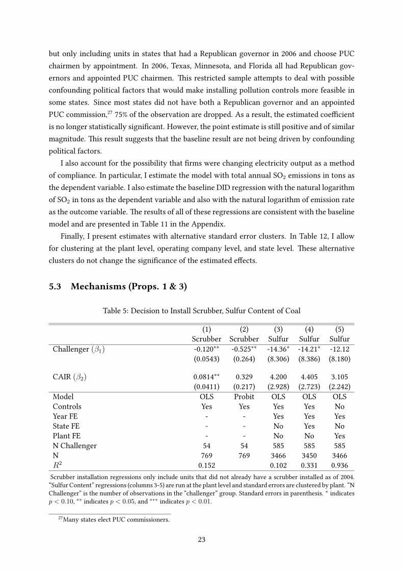
Table 5: Decision to Install Scrubber, Sulfur Content of Coal

(1) (2) (3) (4) (5)

Scrubber Scrubber Sulfur Sulfur Sulfur

Challenger (β1) -0.120∗∗

-0.525∗∗

-14.36∗

-14.21∗

-12.12

(0.0543) (0.264) (8.306) (8.386) (8.180)

CAIR (β2) 0.0814∗∗

0.329 4.200 4.405 3.105

(0.0411) (0.217) (2.928) (2.723) (2.242)

Model OLS Probit OLS OLS OLS

Controls Yes Yes Yes Yes No

Year FE - - Yes Yes Yes

State FE - - No Yes No

Plant FE - - No No Yes

N Challenger 54 54 585 585 585

N 769 769 3466 3450 3466

R20.152 0.102 0.331 0.936

Scrubber installation regressions only include units that did not already have a scrubber installed as of 2004.

“Sulfur Content” regressions (columns 3-5) are run at the plant level and standard errors are clustered by plant. “N

Challenger” is the number of observations in the “challenger” group. Standard errors in parenthesis.∗

indicates

p < 0.10,∗∗

indicates p < 0.05, and∗∗∗

indicates p < 0.01.

27Many states elect PUC commissioners.

23

I now turn to looking at the mechanisms driving the observed di�erences in pollution

abatement. �e �rst two columns of Table 5 contain the estimated e�ects with the scrubber

installation decision as the outcome variable. Units in CAIR states were 8% more likely to

install a scrubber compared to units that were not regulated under CAIR. In addition, units

in “challenger” states were 12% less likely to install a scrubber in comparison to other CAIR

states. �is provides evidence in support of Proposition 1, that �rms with a lower probabil-

ity of being regulated should be less likely to make a sunk investment in pollution-control

technologies.

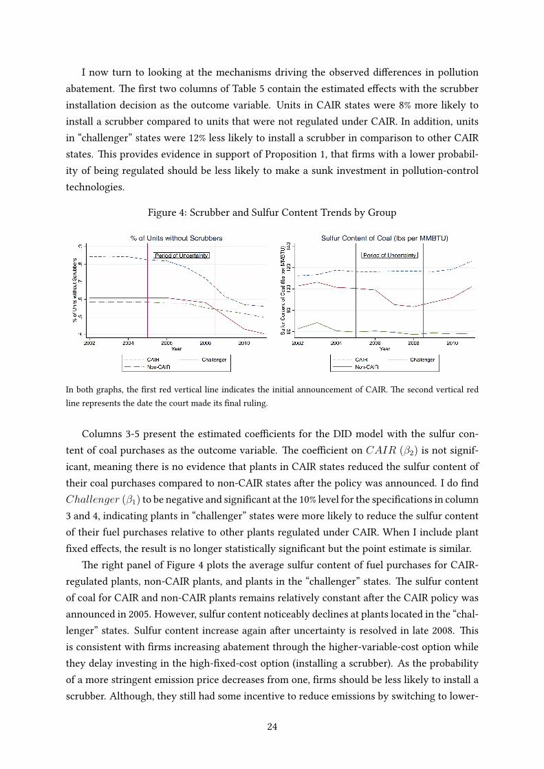
Figure 4: Scrubber and Sulfur Content Trends by Group

In both graphs, the �rst red vertical line indicates the initial announcement of CAIR. �e second vertical red

line represents the date the court made its �nal ruling.

Columns 3-5 present the estimated coe�cients for the DID model with the sulfur con-

tent of coal purchases as the outcome variable. �e coe�cient on CAIR (β2) is not signif-

icant, meaning there is no evidence that plants in CAIR states reduced the sulfur content of

their coal purchases compared to non-CAIR states a�er the policy was announced. I do �nd

Challenger (β1) to be negative and signi�cant at the 10% level for the speci�cations in column

3 and 4, indicating plants in “challenger” states were more likely to reduce the sulfur content

of their fuel purchases relative to other plants regulated under CAIR. When I include plant

�xed e�ects, the result is no longer statistically signi�cant but the point estimate is similar.

�e right panel of Figure 4 plots the average sulfur content of fuel purchases for CAIR-

regulated plants, non-CAIR plants, and plants in the “challenger” states. �e sulfur content

of coal for CAIR and non-CAIR plants remains relatively constant a�er the CAIR policy was

announced in 2005. However, sulfur content noticeably declines at plants located in the “chal-

lenger” states. Sulfur content increase again a�er uncertainty is resolved in late 2008. �is

is consistent with �rms increasing abatement through the higher-variable-cost option while

they delay investing in the high-�xed-cost option (installing a scrubber). As the probability

of a more stringent emission price decreases from one, �rms should be less likely to install a

scrubber. Although, they still had some incentive to reduce emissions by switching to lower-

24

sulfur fuels since permit prices increased a�er the announcement of CAIR.

5.4 Investment A�er the Court Ruling (Prop. 4)

In December 2008, the D.C. Circuit Court ruled that Florida and Texas would be required to

participate in the CAIR program but plants located in Minnesota would be excluded. If plants

were delaying investment to wait for the resolution of the uncertain policy, plants in Texas

and Florida should be more likely to have installed pollution controls in the years immediately

a�er the ruling, while plants in Minnesota would not. Minnesota only had 9 coal units without

pollution controls as of 2009 so it is di�cult to make strong inferences from their behavior;

however, none of these units installed scrubbers in the years immediately following the court

ruling. To test if units in Texas and Florida were more likely to install pollution controls a�er

the �nal ruling, I estimate the model from equation 5. �is regression allows me to identify

how the relative probability of units installing a scrubber in Texas and Florida changed over

time.

Figure 5: Relative Probability of Installing a Scrubber by Year

Estimates of equation 5 are reported in Figure 5. βt can be interpreted as the average addi-

tional probability that units in Texas and Florida installed a scrubber in year t relative to other

units in CAIR. For the years 2007-2009, units in Texas and Florida were less likely to install

scrubbers relative to other CAIR states. A notable change occurs in 2010, β2010 is positive and

signi�cant, meaning units in Texas and Florida were more likely to install scrubbers relative

to other CAIR units. �is is plausibly due to the installations that occurred in response to the

25

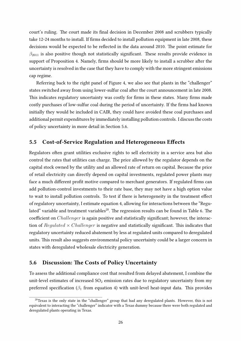
court’s ruling. �e court made its �nal decision in December 2008 and scrubbers typically

take 12-24 months to install. If �rms decided to install pollution equipment in late 2008, these

decisions would be expected to be re�ected in the data around 2010. �e point estimate for

β2011 is also positive though not statistically signi�cant. �ese results provide evidence in

support of Proposition 4. Namely, �rms should be more likely to install a scrubber a�er the

uncertainty is resolved in the case that they have to comply with the more stringent emissions

cap regime.

Referring back to the right panel of Figure 4, we also see that plants in the “challenger”

states switched away from using lower-sulfur coal a�er the court announcement in late 2008.

�is indicates regulatory uncertainty was costly for �rms in these states. Many �rms made

costly purchases of low-sulfur coal during the period of uncertainty. If the �rms had known

initially they would be included in CAIR, they could have avoided these coal purchases and

additional permit expenditures by immediately installing pollution controls. I discuss the costs

of policy uncertainty in more detail in Section 5.6.

5.5 Cost-of-Service Regulation and Heterogeneous E�ects

Regulators o�en grant utilities exclusive rights to sell electricity in a service area but also

control the rates that utilities can charge. �e price allowed by the regulator depends on the

capital stock owned by the utility and an allowed rate of return on capital. Because the price

of retail electricity can directly depend on capital investments, regulated power plants may

face a much di�erent pro�t motive compared to merchant generators. If regulated �rms can

add pollution-control investments to their rate base, they may not have a high option value

to wait to install pollution controls. To test if there is heterogeneity in the treatment e�ect

of regulatory uncertainty, I estimate equation 4, allowing for interactions between the “Regu-

lated” variable and treatment variables28

. �e regression results can be found in Table 6. �e

coe�cient on Challenger is again positive and statistically signi�cant; however, the interac-

tion of Regulated × Challenger is negative and statistically signi�cant. �is indicates that

regulatory uncertainty reduced abatement by less at regulated units compared to deregulated

units. �is result also suggests environmental policy uncertainty could be a larger concern in

states with deregulated wholesale electricity generation.

5.6 Discussion: �e Costs of Policy Uncertainty

To assess the additional compliance cost that resulted from delayed abatement, I combine the

unit-level estimates of increased SO2 emission rates due to regulatory uncertainty from my

preferred speci�cation (β1 from equation 4) with unit-level heat-input data. �is provides

28Texas is the only state in the “challenger” group that had any deregulated plants. However, this is not

equivalent to interacting the “challenger” indicator with a Texas dummy because there were both regulated and

deregulated plants operating in Texas.

26

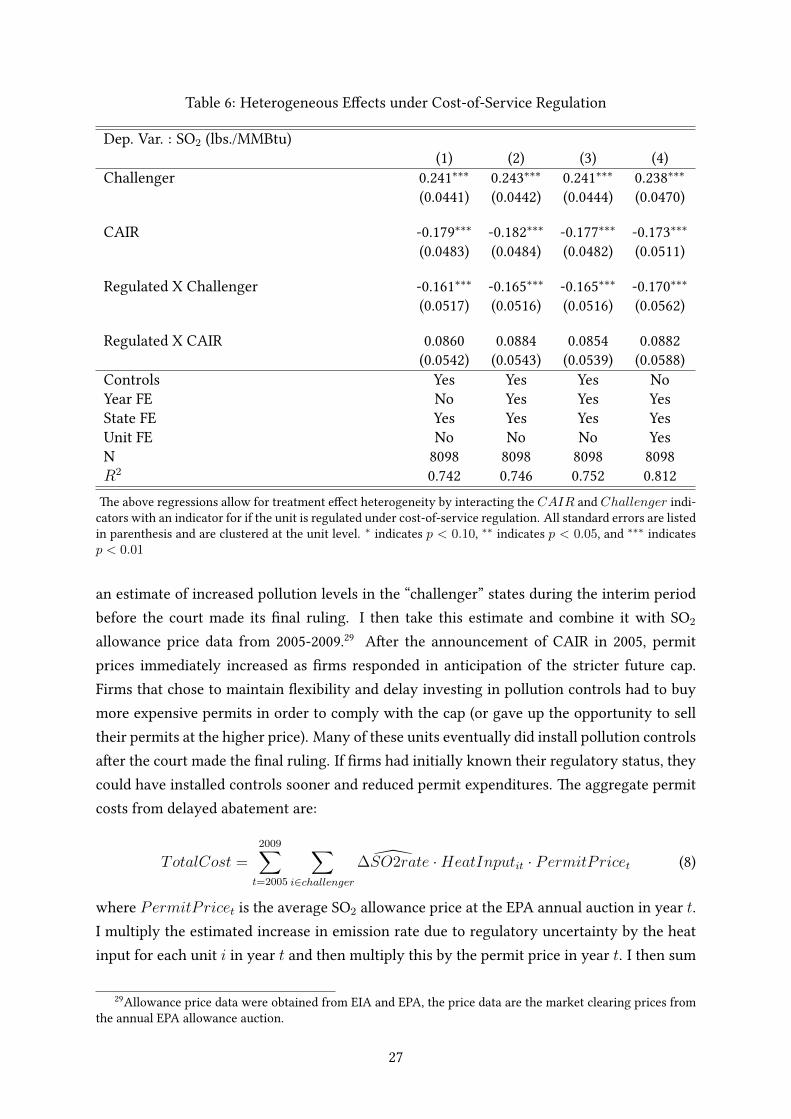
Table 6: Heterogeneous E�ects under Cost-of-Service Regulation

Dep. Var. : SO2 (lbs./MMBtu)

(1) (2) (3) (4)

Challenger 0.241∗∗∗

0.243∗∗∗

0.241∗∗∗

0.238∗∗∗

(0.0441) (0.0442) (0.0444) (0.0470)

CAIR -0.179∗∗∗

-0.182∗∗∗

-0.177∗∗∗

-0.173∗∗∗

(0.0483) (0.0484) (0.0482) (0.0511)

Regulated X Challenger -0.161∗∗∗

-0.165∗∗∗

-0.165∗∗∗

-0.170∗∗∗

(0.0517) (0.0516) (0.0516) (0.0562)

Regulated X CAIR 0.0860 0.0884 0.0854 0.0882

(0.0542) (0.0543) (0.0539) (0.0588)

Controls Yes Yes Yes No

Year FE No Yes Yes Yes

State FE Yes Yes Yes Yes

Unit FE No No No Yes

N 8098 8098 8098 8098

R20.742 0.746 0.752 0.812

�e above regressions allow for treatment e�ect heterogeneity by interacting the CAIR and Challenger indi-

cators with an indicator for if the unit is regulated under cost-of-service regulation. All standard errors are listed

in parenthesis and are clustered at the unit level.∗

indicates p < 0.10,∗∗

indicates p < 0.05, and∗∗∗

indicates

p < 0.01

an estimate of increased pollution levels in the “challenger” states during the interim period

before the court made its �nal ruling. I then take this estimate and combine it with SO2

allowance price data from 2005-2009.29

A�er the announcement of CAIR in 2005, permit

prices immediately increased as �rms responded in anticipation of the stricter future cap.

Firms that chose to maintain �exibility and delay investing in pollution controls had to buy

more expensive permits in order to comply with the cap (or gave up the opportunity to sell

their permits at the higher price). Many of these units eventually did install pollution controls

a�er the court made the �nal ruling. If �rms had initially known their regulatory status, they

could have installed controls sooner and reduced permit expenditures. �e aggregate permit

costs from delayed abatement are:

TotalCost =2009∑t=2005

∑i∈challenger

∆SO2rate ·HeatInputit · PermitPricet (8)

where PermitPricet is the average SO2 allowance price at the EPA annual auction in year t.

I multiply the estimated increase in emission rate due to regulatory uncertainty by the heat

input for each unit i in year t and then multiply this by the permit price in year t. I then sum

29Allowance price data were obtained from EIA and EPA, the price data are the market clearing prices from

the annual EPA allowance auction.

27

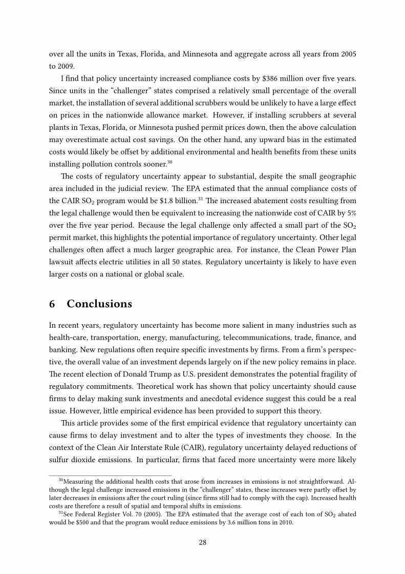
over all the units in Texas, Florida, and Minnesota and aggregate across all years from 2005

to 2009.

I �nd that policy uncertainty increased compliance costs by $386 million over �ve years.

Since units in the “challenger” states comprised a relatively small percentage of the overall

market, the installation of several additional scrubbers would be unlikely to have a large e�ect

on prices in the nationwide allowance market. However, if installing scrubbers at several

plants in Texas, Florida, or Minnesota pushed permit prices down, then the above calculation

may overestimate actual cost savings. On the other hand, any upward bias in the estimated

costs would likely be o�set by additional environmental and health bene�ts from these units

installing pollution controls sooner.30

�e costs of regulatory uncertainty appear to substantial, despite the small geographic

area included in the judicial review. �e EPA estimated that the annual compliance costs of

the CAIR SO2 program would be $1.8 billion.31

�e increased abatement costs resulting from

the legal challenge would then be equivalent to increasing the nationwide cost of CAIR by 5%

over the �ve year period. Because the legal challenge only a�ected a small part of the SO2

permit market, this highlights the potential importance of regulatory uncertainty. Other legal

challenges o�en a�ect a much larger geographic area. For instance, the Clean Power Plan

lawsuit a�ects electric utilities in all 50 states. Regulatory uncertainty is likely to have even

larger costs on a national or global scale.

6 Conclusions

In recent years, regulatory uncertainty has become more salient in many industries such as

health-care, transportation, energy, manufacturing, telecommunications, trade, �nance, and

banking. New regulations o�en require speci�c investments by �rms. From a �rm’s perspec-

tive, the overall value of an investment depends largely on if the new policy remains in place.

�e recent election of Donald Trump as U.S. president demonstrates the potential fragility of

regulatory commitments. �eoretical work has shown that policy uncertainty should cause

�rms to delay making sunk investments and anecdotal evidence suggest this could be a real

issue. However, li�le empirical evidence has been provided to support this theory.

�is article provides some of the �rst empirical evidence that regulatory uncertainty can

cause �rms to delay investment and to alter the types of investments they choose. In the

context of the Clean Air Interstate Rule (CAIR), regulatory uncertainty delayed reductions of

sulfur dioxide emissions. In particular, �rms that faced more uncertainty were more likely

30Measuring the additional health costs that arose from increases in emissions is not straightforward. Al-

though the legal challenge increased emissions in the “challenger” states, these increases were partly o�set by

later decreases in emissions a�er the court ruling (since �rms still had to comply with the cap). Increased health

costs are therefore a result of spatial and temporal shi�s in emissions.

31See Federal Register Vol. 70 (2005). �e EPA estimated that the average cost of each ton of SO2 abated

would be $500 and that the program would reduce emissions by 3.6 million tons in 2010.

28

to delay investment in capital infrastructure to reduce emissions. Furthermore, these �rms

were more likely to use abatement strategies that didn’t require large �xed costs. In order

to maintain �exibility many �rms decided to purchase emissions allowances as a means of

compliance. I estimate delayed investment stemming from regulatory uncertainty increased

�rm’s expenditures on allowances by $386 million.

In order to address concerns about climate change, new regulations will need to be intro-

duced and existing policies will need to be updated in the energy sector and other industrial

sectors. In the United States, the EPA proposed the Clean Power Plan in 2014 as a potential

policy to reduce greenhouse gas emissions from the electricity sector. �e policy would re-

quire substantial investment in renewable and natural gas generation and the retirement of

many existing coal plants. However, the long-term implementation of the Clean Power Plan

remains largely uncertain due to unknown future political conditions and unknown outcomes

of the judicial review process. Many states initially �led lawsuits challenging the legality of

the policy. �ese lawsuits culminated in the Supreme Court ordering the EPA to halt en-

forcement of the rule. Now the rule must be reviewed again in court and could be altered or

scrapped by the new Trump administration. In the end, it could be several years between the

proposal of the policy and the time when �rms actually know the �nal status and details of

the regulation. We have seen that this political and legal uncertainty could hinder the e�ec-

tiveness of government policies that aim to spur investment in cleaner capital infrastructure.

29

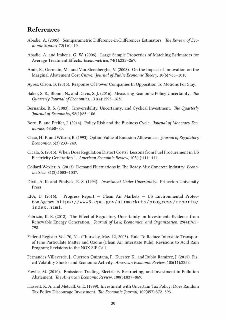
ReferencesAbadie, A. (2005). Semiparametric Di�erence-in-Di�erences Estimators. �e Review of Eco-nomic Studies, 72(1):1–19.

Abadie, A. and Imbens, G. W. (2006). Large Sample Properties of Matching Estimators for

Average Treatment E�ects. Econometrica, 74(1):235–267.

Amir, R., Germain, M., and Van Steenberghe, V. (2008). On the Impact of Innovation on the

Marginal Abatement Cost Curve. Journal of Public Economic �eory, 10(6):985–1010.

Ayres, Olson, B. (2015). Response Of Power Companies In Opposition To Motions For Stay.

Baker, S. R., Bloom, N., and Davis, S. J. (2016). Measuring Economic Policy Uncertainty. �e�arterly Journal of Economics, 131(4):1593–1636.

Bernanke, B. S. (1983). Irreversibility, Uncertainty, and Cyclical Investment. �e �arterlyJournal of Economics, 98(1):85–106.

Born, B. and Pfeifer, J. (2014). Policy Risk and the Business Cycle. Journal of Monetary Eco-nomics, 68:68–85.

Chao, H.-P. and Wilson, R. (1993). Option Value of Emission Allowances. Journal of RegulatoryEconomics, 5(3):233–249.

Cicala, S. (2015). When Does Regulation Distort Costs? Lessons from Fuel Procurement in US

Electricity Generation†. American Economic Review, 105(1):411–444.

Collard-Wexler, A. (2013). Demand Fluctuations In �e Ready-Mix Concrete Industry. Econo-metrica, 81(3):1003–1037.

Dixit, A. K. and Pindyck, R. S. (1994). Investment Under Uncertainty. Princeton University

Press.

EPA, U. (2016). Progress Report — Clean Air Markets — US Environmental Protec-

tion Agency. https://www3.epa.gov/airmarkets/progress/reports/index.html.

Fabrizio, K. R. (2012). �e E�ect of Regulatory Uncertainty on Investment: Evidence from

Renewable Energy Generation. Journal of Law, Economics, and Organization, 29(4):765–

798.

Federal Register Vol. 70, N. . (�ursday, May 12, 2005). Rule To Reduce Interstate Transport

of Fine Particulate Ma�er and Ozone (Clean Air Interstate Rule); Revisions to Acid Rain

Program; Revisions to the NOX SIP Call.

Fernandez-Villaverde, J., Guerron-�intana, P., Kuester, K., and Rubio-Ramirez, J. (2015). Fis-

cal Volatility Shocks and Economic Activity. American Economic Review, 105(11):3352.

Fowlie, M. (2010). Emissions Trading, Electricity Restructing, and Investment in Pollution

Abatement. �e American Economic Review, 100(3):837–869.

Hasse�, K. A. and Metcalf, G. E. (1999). Investment with Uncertain Tax Policy: Does Random

Tax Policy Discourage Investment. �e Economic Journal, 109(457):372–393.

30

Hurn, A. S. and Wright, R. E. (1994). Geology or Economics? Testing Models of Irreversible

Investment Using North Sea Oil Data. �e Economic Journal, 104(423):363–371.

Jung, C., Krutilla, K., and Boyd, R. (1996). Incentives for Advanced Pollution Abatement Tech-

nology at the Industry Level: An Evaluation of Policy Alternatives. Journal of EnvironmentalEconomics and Management, 30(1):95–111.

Kellogg, R. (2014). �e E�ect of Uncertainty on Investment: Evidence from Texas Oil Drilling.

American Economic Review, 104(6):1698–1734.

Kelly, B., Pastor, L., and Veronesi, P. (2014). �e Price of Political Uncertainty: �eory and

Evidence from the Option Market. Technical report, National Bureau of Economic Research.

Kruse, E. (2009). North Carolina v. Environmental Protection Agency. Harv. Envtl. L. Rev.,33:283.

Krysiak, F. C. (2008). Prices Vs. �antities: �e E�ects on Technology Choice. Journal ofPublic Economics, 92(5–6):1275–1287.

La�ont, J.-J. and Tirole, J. (1996). Pollution Permits and Compliance Strategies. Journal ofPublic Economics, 62(1):85–125.

List, J. A. and Haigh, M. S. (2010). Investment Under Uncertainty: Testing �e Options Model

With Professional Traders. �e Review of Economics and Statistics, 92(4):974–984.

McDonald, R. and Siegel, D. (1986). �e Value of Waiting to Invest. �e �arterly Journal ofEconomics, 101(4):707–728.

Milliman, S. R. and Prince, R. (1989). Firm Incentives to Promote Technological Change in

Pollution Control. Journal of Environmental economics and Management, 17(3):247–265.

Moel, A. and Tufano, P. (2002). When Are Real Options Exercised? An Empirical Study of

Mine Closings. Review of Financial Studies, 15(1):35–64.

Pakes, A. (1986). Patents as Options: Some Estimates of the Value of Holding European Patent

Stocks. Econometrica, 54(4):755–784.

Pastor, L. and Veronesi, P. (2013). Political Uncertainty and Risk Premia. Journal of FinancialEconomics, 110(3):520–545.

Pindyck, R. S. (1988). Irreversible Investment, Capacity Choice, and the Value of the Firm. �eAmerican Economic Review, 78(5):969–985.

Requate, T. (2005). Timing and Commitment of Environmental Policy, Adoption of New Tech-

nology, and Repercussions on R&D. Environmental and Resource Economics, 31(2):175–199.

Requate, T. and Unold, W. (2003). Environmental Policy Incentives to Adopt Advanced Abate-

ment Technology:: Will the True Ranking Please stand Up? European Economic Review,

47(1):125–146.

Rodrik, D. (1991). Policy Uncertainty and Private Investment in Developing Countries. Journalof Development Economics, 36(2):229–242.

31

Schmalensee, R. and Stavins, R. N. (2013). �e SO2 Allowance Trading System: �e Ironic

History of a Grand Policy Experiment. �e Journal of Economic Perspectives, 27(1):103–121.

Stokey, N. L. (2016). Wait-and-See: Investment Options Under Policy Uncertainty. Review ofEconomic Dynamics, 21:246–265.

Teisberg, E. O. (1993). Capital Investment Strategies Under Uncertain Regulation. �e RANDJournal of Economics, 24(4):591–604.

Zhao, J. (2003). Irreversible Abatement Investment Under Cost Uncertainties: Tradable Emis-

sion Permits and Emissions Charges. Journal of Public Economics, 87(12):2765–2789.

Appendices

A Judicial Review: North Carolina vs. EPA

�is section provides additional details on CAIR and the judicial review of the program. All

challenges to the CAIR program were combined into a single case: North Carolina vs. EPA.32

�e CAIR rule was initially introduced in 2005 to aid several states in complying with

National Ambient Air �ality Standards (NAAQS) required under the Clean Air Act. NAAQS

were initially imposed to reduce ambient levels of particulate ma�er, ground-level ozone and

other pollutants. �ese pollutants can be harmful to human health and can damage both

agriculture and natural ecosystems. Ozone levels can be di�cult to regulate locally because

several precursors to ozone such as SO2 and NOx can be generated from sources in other states.

�e EPA introduced CAIR in order to limit SO2 and NOx emissions that were contributing

to non-a�ainment of air quality standards in many downwind states. �e program would

require emission reductions from most eastern states. States that were regulated under CAIR

could propose their own plan for compliance or join the new CAIR cap and trade program for

electric generating units that would be administered by the EPA.

North Carolina, as well as several other states and electric utility companies challenged

the legality of the CAIR rule a�er its announcement in 2005. �e D.C. Circuit Court of Appeals

separated legal challenges into four di�erent categories: (1) SO2 and NOx budgets (2) altering

the allocation of Title IV allowances (3) the exclusion of some border states (4) the Phase I

compliance deadline.

�is article focuses on the uncertainty generated by the third category, the exclusion of

some border states. Although there was uncertainty generated by all four categories of North

Carolina vs. EPA, the exclusion of border states challenge is the only category that di�eren-

tiated some plants in their probability of being regulated.

32See Kruse (2009) for an even more comprehensive background.

32

In July 2008, the D.C. Circuit Court agreed with parts of three of the four arguments from

North Carolina. �e court ruled that CAIR was unlawful under the Clean Air Act because it

did not speci�cally address any one state’s contribution to another individual states ambient

air quality. Instead it formulated emission reductions as a group, meaning any particular state

could avoid making actual emission reductions by instead purchasing permits from the cap

and trade pool.

�e court also ruled in response to utility objections to SO2 and NOx budgets under CAIR.

�ey ruled that the EPA’s allocation rules did not speci�cally target pollution reduction in

speci�c upwind states. Furthermore, the EPA had initially proposed reducing SO2 permit

allocations from the Title IV Acid Rain program. However, the court decided that the EPA did

not have authority to reduce �rm’s allocations of Title IV permits or to remove permits from

circulation. �e court also ruled that the Phase 1 of CAIR did not require su�cient emission

reductions that were required by 2010 under the Clean Air Act.

�e court also approved one border state challenge, the motion to exclude Minnesota;

however, they rejected the motions to exclude Texas and Florida. �e court ruled that the

EPA had not provided su�cient evidence of Minnesota’s contribution of non-compliance for

downwind states.

A�er an initial court ruling in July 2008, it appeared that CAIR SO2 would not be imple-

mented in 2010 as planned. �e EPA would need to signi�cantly change many of the CAIR

provisions in order for it to become law. However, in December 2008, the D.C. Circuit Court

decided that both the CAIR SO2 and NOx programs would proceed as scheduled and remain

in place while the EPA constructed a new rule to replace CAIR. �e court did not provide a

de�nitive time table for EPA to complete the new replacement regulation.

All states that were initially scheduled to participate in the CAIR SO2 program with the

exception of Minnesota were forced to comply with CAIR during the period of 2010-2014. In

2015, phase 1 of a replacement program called the Cross-State Air Pollution Rule went into

e�ect. �e Cross-State Air Pollution Rule addressed the court’s initial concerns by limiting

permit trading to within speci�c air basins and not altering allocations of Title IV permits.

B Proofs of Propositions

To simply exposition, I assume without loss of generality that the the discount rate r = 0.

�e �rms problem in the �rst period can then be wri�en as:

min

a1,I1P1 · (e− a1) + C(a1, I1) +K · I1 + E

[min

a2,I2{P2 · (e− a2) + C(a2, I2) +K · (I2 − I1)}

]s.t. at ∈ [0, e], It ∈ {0, 1}, I2 ≥ I1

33

B.1 Proof of Proposition 1

Firms are di�erentiated by their costs of capital. Speci�cally, there are three groups of �rms:

(1) �rms that will install the capital technology in the �rst period, (2) �rms that will wait to

install the capital technology only if the high emissions price is realized, (3) and a group of

�rms that will never install the capital technology. �e third group will have the highest cost

of capital and regardless of ρ they will never install the technology. �erefore, the share of

�rm’s adopting the technology in the �rst period will be determined by the cuto� capital cost

K∗1 that separates the �rst and second groups. I will show that K∗1 is increasing in ρ and

therefore the the share of adopters in period one F (K∗1) will also be increasing in ρ.

�e expected net bene�ts from installing in period 1 are equal to: P1 · aI1 − C(aI1, 1) −K +E[min{P2 · a2−C(a2, 1)}|I1 = 1].33

If the �rm installs the technology in period 1, they

save on permit costs and abatement costs in period 1 and anticipate saving on permit costs and

abatement costs in period 2; however, they also must pay the capital costK and the abatement

cost C(aI1, 1). If the �rm waits until period 2 and only installs the capital technology if the

stringent price is enacted, then their expected bene�t will be P1 ·aN1 −C(aN1 , 0)+E[min{P2 ·a2 − C(a2, I2) +K · I2}|I1 = 0]. Firms should invest if:

P1 · aI1 − C(aI1, 1)−K + E[min

a2,I2{P2 · a2 − C(a2, I2)}|I1 = 1]

≥ P1 · aN1 − C(aN1 , 0) + E[min

a2,I2{P2 · a2 − C(a2, I2) +K · I2}|I1 = 0]

(9)

Let aIH2 be the optimal level of abatement in period 2, conditional on having installed the

capital technology (I2 = 1) and emission prices being high. Let aIL2 be the optimal abatement

level if permit prices are low and the �rm has installed the technology. Furthermore, let aNH2

and aNL2 be the optimal abatement levels for �rms who have not installed the technology for

the high and low emission price cases respectively. Expanding the expectations, we have:

P1 · aI1 − C(aI1, 1)−K + ρ(PH2 · aIH2 − C(aIH2 , 1))

+(1− ρ)(PL2 · aIL2 − C(aIL2 , 1)) ≥ P1 · aN1 − C(aN1 , 0)

+ρ(PH2 · aIH2 − C(aIH2 , 1)−K) + (1− ρ)(PL

2 · aNL2 − C(aNL2 , 0))

(10)

To understand the the right-hand side of the inequality, recall that �rms in the second group

will install the capital technology in the second period only if the high permit price is realized,

which will occur with probability ρ. �e cuto� cost K∗1 for investment in the �rst period is

determined by the capital cost at which a �rm would be indi�erent between investing and

waiting. Se�ing the right and le� hand sides of (10) equal to each other and solving for K we

obtain:

33Recall aI1 is the optimal �rst period abatement conditional on installing the capital technology, and aN1 is

the optimal �rst period abatement choice for �rms that do not install the technology.

34

K∗1 =

(P1 · aI1 − C(aI1, 1)

)−(P1 · aN1 − C(aN1 , 0)

)1− ρ

+(PL

2 · aIL2 − C(aIL2 , 1))−(PL

2 · aNL2 − C(aNL2 , 0)) (11)

di�erentiating (11) with respect to ρ we have:

dK∗1dρ

=P1

1− ρ

(daI1dρ− daN1

dρ

)+

1

1− ρ

(Ca(a

N1 , 0)

daN1dρ− Ca(aI1, 1)

daI1dρ

)+

1

(1− ρ)2

([P1 · aI1 − C(aI1, 1)]− [P1 · aN1 − C(aN1 , 0)]

)+ PL

2

(daIL2dρ− daNL2

dρ

)+(Ca(a

NL2 , 0)

daNL2

dρ− Ca(aIL2 , 1)

daIL2dρ

) (12)

Substituting in the equilibrium conditions, Ca(a1, I1) = P1 and Ca(a2, I2) = P2, and cancel-

ing terms we are le� with:

dK∗1dρ

=1

(1− ρ)2

([P1 · aI1 − C(aI1, 1)]− [P1 · aN1 − C(aN1 , 0)]

)(13)

We know that the �rst term in brackets must be larger than the second term in brackets. To

see this, notice P1 ·aI1−C(aI1, 1) ≥ P1 ·aN1 −C(aN1 , 1) since aI1 is the optimal abatement choice

conditional on having I1 = 1 by de�nition. Additionally we know that P1 · aN1 −C(aN1 , 1) >

P1 · aN1 − C(aN1 , 0) which follows from the assumption that marginal cost of abatement is

lower once the capital technology is installed. �is means the term in the large parentheses

is positive, and since1

(1−ρ)2is positive this implies

dK∗1

dρ> 0. Finally, since the cumulative

distribution function F must be non-decreasing in its argument it follows thatdF (K∗

1 )

dρ≥ 0

�

B.2 Proof of Proposition 2

We will show thatde1dρ

< 0. Total emissions is equal to the sum of emissions from �rms that

invest in the technology and emissions from those that do not:

e1 = M(F (K∗1)(e− aI1) + (1− F (K∗1))(e− aN1 )

)(14)

We next di�erentiate with respect to ρ to obtain a comparative static:

de1dρ

= M[f(K∗)

dK∗

dρ((e− aI1)− (e− aN1 ))− F (K∗)

daI1dρ− (1− F (K∗))

daN1dρ

](15)

where f is the probability density function of K . We know that the �rst term in the

brackets, f(K∗)dK∗

dρ((e − aI1) − (e − aN1 )), is negative since f is non-negative by de�nition,

35

dF (K∗1 )

dρis positive as shown above, and ((e − aI1) − (e − aN1 )) is negative because �rms that

install the technology will have lower emissions. �e next two terms in the brackets are equal

to zero becausedaI1dρ

= 0 anddaN1dρ

= 0, this can be shown by di�erentiating the �rst order

condition Ca(a1, I1) = P1 with respect to ρ. �erefore, since M is also non-negative, it must

be the case thatde1dρ≤ 0.

�

B.3 Proof of Proposition 3

Let aN1 denote total abatement by �rms that do not adopt the technology in the �rst period,

aN1 =

∑i ai1 · 1(Ii1 = 0). Total abatement by non-adopters is equal to:

aN1 = M(

(1− F (K∗1))(aN1 ))

(16)

Di�erentiating with respect to ρ we have:

daN1dρ

= M[−f(K∗1)

dK∗1

dρ(aN1 )︸ ︷︷ ︸

[1]

+ (1− F (K∗1))daN1dρ︸ ︷︷ ︸

[2]

](17)

As the probability of the high price regime increases, more �rms adopt the technology,

which works to reduce total abatement by no adopters, this e�ect is labeled [1] in equation

17. �is term is negative since f(K∗1), aN1 are positive anddK∗

1

dρis positive by proposition 1.

SincedaN1dρ

= 0, the term labeled [2] in equation 17 equals zero. �erefore,daN

1

dρ≤ 0.

B.4 Proof of Proposition 4

De�ne K∗2 as the the cuto� capital cost that a �rm would be indi�erent to installing the tech-

nology in the second period, conditional on the high price regime occurring:

K∗2 = (PH2 · aIH2 − C(aIH2 , 1))− (PH

2 · aNH2 − C(aNH2 , 0)) (18)

Notice the cuto� does not depend on ρ since the uncertainty has already been resolved

at this point. �e number of �rms that adopt is the number of �rms that have capital costs

smaller than K∗2 but have capital costs larger than K∗1 (i.e., did not invest in the �rst period).

�is number of �rms can be expressed as:

M ∗max{0, (F (K∗2)− F (K∗1))} (19)

Let ρ be de�ned such that K∗2 = K∗1(ρ). �en di�erentiating (19) we obtain:

d[M ∗max{0, (F (K∗2)− F (K∗1(ρ)))}]dρ

=

0, if ρ > ρ

M(−f(K∗1)dK∗

1

dρ), if ρ < ρ

(20)

36

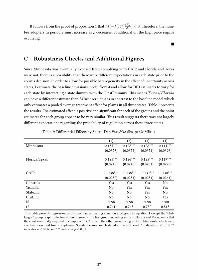
It follows from the proof of proposition 1 that M(−f(K∗1)dK∗

1

dρ) < 0. �erefore, the num-

ber adopters in period 2 must increase as ρ decreases, conditional on the high price regime

occurring.

�

C Robustness Checks and Additional Figures

Since Minnesota was eventually excused from complying with CAIR and Florida and Texas

were not, there is a possibility that there were di�erent expectations in each state prior to the

court’s decision. In order to allow for possible heterogeneity in the e�ect of uncertainty across

states, I estimate the baseline emissions model from 4 and allow for DID estimates to vary for

each state by interacting a state dummy with the ”Post” dummy. �is means Texas/F lorida

can have a di�erent estimate than Minnesota, this is in contrast to the baseline model which

only estimates a pooled average treatment e�ect for plants in all three states. Table 7 presents

the results. �e estimated e�ect is positive and signi�cant for each of the groups and the point

estimates for each group appear to be very similar. �is result suggests there was not largely

di�erent expectations regarding the probability of regulation across these three states.

Table 7: Di�erential E�ects by State - Dep Var: SO2 (lbs. per MMBtu)

(1) (2) (3) (4)

Minnesota 0.133∗∗∗

0.128∗∗∗

0.128∗∗∗

0.114∗∗∗

(0.0378) (0.0372) (0.0374) (0.0396)

Florida/Texas 0.125∗∗∗

0.126∗∗∗

0.125∗∗∗

0.119∗∗∗

(0.0248) (0.0248) (0.0251) (0.0278)

CAIR -0.138∗∗∗

-0.138∗∗∗

-0.137∗∗∗

-0.130∗∗∗

(0.0230) (0.0231) (0.0234) (0.0261)

Controls Yes Yes Yes No

Year FE No Yes Yes Yes

State FE No No Yes No

Unit FE No No No Yes

N 8098 8098 8098 8280

r2 0.741 0.745 0.750 0.818

�is table presents regression results from an estimating equation analogous to equation 4 except the “chal-

lenger” group is split into two di�erent groups: the �rst group including units in Florida and Texas, units that

the court eventually required to comply with CAIR, and the other group being units in Minnesota which were

eventually excused from compliance. Standard errors are clustered at the unit level.∗

indicates p < 0.10,∗∗

indicates p < 0.05, and∗∗∗

indicates p < 0.01

37

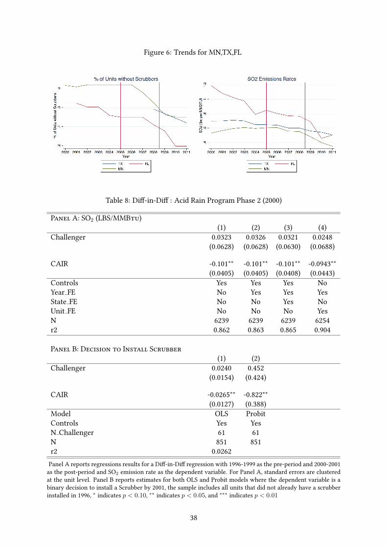
Figure 6: Trends for MN,TX,FL

Table 8: Di�-in-Di� : Acid Rain Program Phase 2 (2000)

Panel A: SO2 (LBS/MMBtu)

(1) (2) (3) (4)

Challenger 0.0323 0.0326 0.0321 0.0248

(0.0628) (0.0628) (0.0630) (0.0688)

CAIR -0.101∗∗

-0.101∗∗

-0.101∗∗

-0.0943∗∗

(0.0405) (0.0405) (0.0408) (0.0443)

Controls Yes Yes Yes No

Year FE No Yes Yes Yes

State FE No No Yes No

Unit FE No No No Yes

N 6239 6239 6239 6254

r2 0.862 0.863 0.865 0.904

Panel B: Decision to Install Scrubber

(1) (2)

Challenger 0.0240 0.452

(0.0154) (0.424)

CAIR -0.0265∗∗

-0.822∗∗

(0.0127) (0.388)

Model OLS Probit

Controls Yes Yes

N Challenger 61 61

N 851 851

r2 0.0262

Panel A reports regressions results for a Di�-in-Di� regression with 1996-1999 as the pre-period and 2000-2001

as the post-period and SO2 emission rate as the dependent variable. For Panel A, standard errors are clustered

at the unit level. Panel B reports estimates for both OLS and Probit models where the dependent variable is a

binary decision to install a Scrubber by 2001, the sample includes all units that did not already have a scrubber

installed in 1996,∗

indicates p < 0.10,∗∗

indicates p < 0.05, and∗∗∗

indicates p < 0.01

38

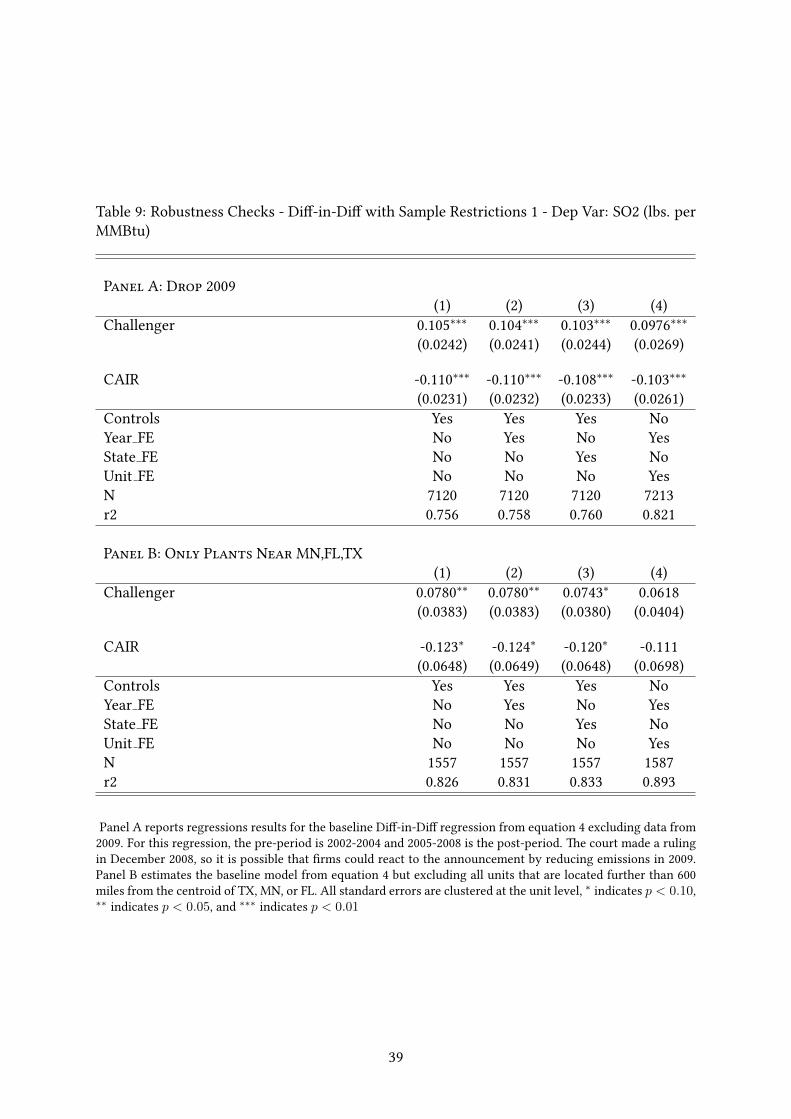
Table 9: Robustness Checks - Di�-in-Di� with Sample Restrictions 1 - Dep Var: SO2 (lbs. per

MMBtu)

Panel A: Drop 2009

(1) (2) (3) (4)

Challenger 0.105∗∗∗

0.104∗∗∗

0.103∗∗∗

0.0976∗∗∗

(0.0242) (0.0241) (0.0244) (0.0269)

CAIR -0.110∗∗∗

-0.110∗∗∗

-0.108∗∗∗

-0.103∗∗∗

(0.0231) (0.0232) (0.0233) (0.0261)

Controls Yes Yes Yes No

Year FE No Yes No Yes

State FE No No Yes No

Unit FE No No No Yes

N 7120 7120 7120 7213

r2 0.756 0.758 0.760 0.821

Panel B: Only Plants Near MN,FL,TX

(1) (2) (3) (4)

Challenger 0.0780∗∗

0.0780∗∗

0.0743∗

0.0618

(0.0383) (0.0383) (0.0380) (0.0404)

CAIR -0.123∗

-0.124∗

-0.120∗

-0.111

(0.0648) (0.0649) (0.0648) (0.0698)

Controls Yes Yes Yes No

Year FE No Yes No Yes

State FE No No Yes No

Unit FE No No No Yes

N 1557 1557 1557 1587

r2 0.826 0.831 0.833 0.893

Panel A reports regressions results for the baseline Di�-in-Di� regression from equation 4 excluding data from

2009. For this regression, the pre-period is 2002-2004 and 2005-2008 is the post-period. �e court made a ruling

in December 2008, so it is possible that �rms could react to the announcement by reducing emissions in 2009.

Panel B estimates the baseline model from equation 4 but excluding all units that are located further than 600

miles from the centroid of TX, MN, or FL. All standard errors are clustered at the unit level,∗

indicates p < 0.10,

∗∗indicates p < 0.05, and

∗∗∗indicates p < 0.01

39

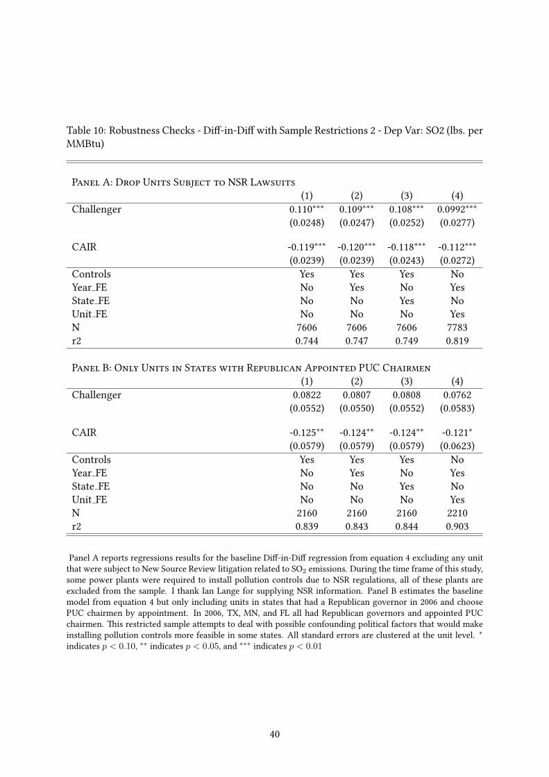
Table 10: Robustness Checks - Di�-in-Di� with Sample Restrictions 2 - Dep Var: SO2 (lbs. per

MMBtu)

Panel A: Drop Units Subject to NSR Lawsuits

(1) (2) (3) (4)

Challenger 0.110∗∗∗

0.109∗∗∗

0.108∗∗∗

0.0992∗∗∗

(0.0248) (0.0247) (0.0252) (0.0277)

CAIR -0.119∗∗∗

-0.120∗∗∗

-0.118∗∗∗

-0.112∗∗∗

(0.0239) (0.0239) (0.0243) (0.0272)

Controls Yes Yes Yes No

Year FE No Yes No Yes

State FE No No Yes No

Unit FE No No No Yes

N 7606 7606 7606 7783

r2 0.744 0.747 0.749 0.819

Panel B: Only Units in States with Republican Appointed PUC Chairmen

(1) (2) (3) (4)

Challenger 0.0822 0.0807 0.0808 0.0762

(0.0552) (0.0550) (0.0552) (0.0583)

CAIR -0.125∗∗

-0.124∗∗

-0.124∗∗

-0.121∗

(0.0579) (0.0579) (0.0579) (0.0623)

Controls Yes Yes Yes No

Year FE No Yes No Yes

State FE No No Yes No

Unit FE No No No Yes

N 2160 2160 2160 2210

r2 0.839 0.843 0.844 0.903

Panel A reports regressions results for the baseline Di�-in-Di� regression from equation 4 excluding any unit

that were subject to New Source Review litigation related to SO2 emissions. During the time frame of this study,

some power plants were required to install pollution controls due to NSR regulations, all of these plants are

excluded from the sample. I thank Ian Lange for supplying NSR information. Panel B estimates the baseline

model from equation 4 but only including units in states that had a Republican governor in 2006 and choose

PUC chairmen by appointment. In 2006, TX, MN, and FL all had Republican governors and appointed PUC

chairmen. �is restricted sample a�empts to deal with possible confounding political factors that would make

installing pollution controls more feasible in some states. All standard errors are clustered at the unit level.∗

indicates p < 0.10,∗∗

indicates p < 0.05, and∗∗∗

indicates p < 0.01

40

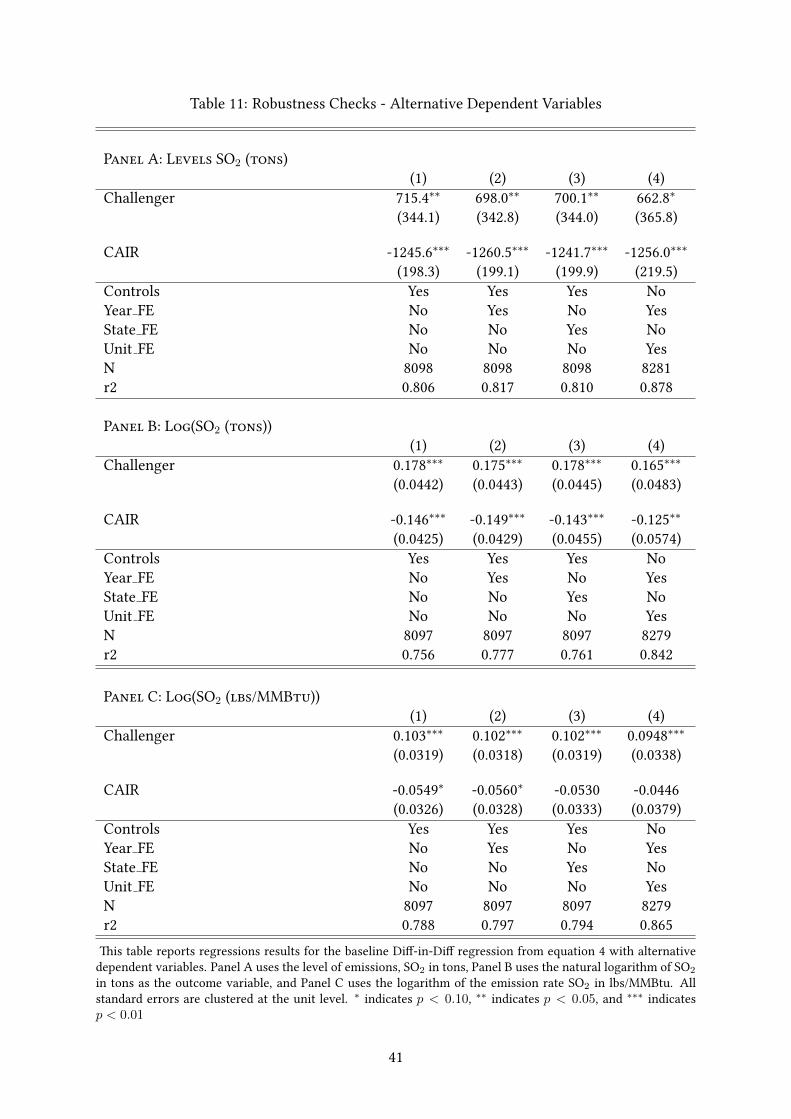
Table 11: Robustness Checks - Alternative Dependent Variables

Panel A: Levels SO2 (tons)

(1) (2) (3) (4)

Challenger 715.4∗∗

698.0∗∗

700.1∗∗

662.8∗

(344.1) (342.8) (344.0) (365.8)

CAIR -1245.6∗∗∗

-1260.5∗∗∗

-1241.7∗∗∗

-1256.0∗∗∗

(198.3) (199.1) (199.9) (219.5)

Controls Yes Yes Yes No

Year FE No Yes No Yes

State FE No No Yes No

Unit FE No No No Yes

N 8098 8098 8098 8281

r2 0.806 0.817 0.810 0.878

Panel B: Log(SO2 (tons))

(1) (2) (3) (4)

Challenger 0.178∗∗∗

0.175∗∗∗

0.178∗∗∗

0.165∗∗∗

(0.0442) (0.0443) (0.0445) (0.0483)

CAIR -0.146∗∗∗

-0.149∗∗∗

-0.143∗∗∗

-0.125∗∗

(0.0425) (0.0429) (0.0455) (0.0574)

Controls Yes Yes Yes No

Year FE No Yes No Yes

State FE No No Yes No

Unit FE No No No Yes

N 8097 8097 8097 8279

r2 0.756 0.777 0.761 0.842

Panel C: Log(SO2 (lbs/MMBtu))

(1) (2) (3) (4)

Challenger 0.103∗∗∗

0.102∗∗∗

0.102∗∗∗

0.0948∗∗∗

(0.0319) (0.0318) (0.0319) (0.0338)

CAIR -0.0549∗

-0.0560∗

-0.0530 -0.0446

(0.0326) (0.0328) (0.0333) (0.0379)

Controls Yes Yes Yes No

Year FE No Yes No Yes

State FE No No Yes No

Unit FE No No No Yes

N 8097 8097 8097 8279

r2 0.788 0.797 0.794 0.865

�is table reports regressions results for the baseline Di�-in-Di� regression from equation 4 with alternative

dependent variables. Panel A uses the level of emissions, SO2 in tons, Panel B uses the natural logarithm of SO2

in tons as the outcome variable, and Panel C uses the logarithm of the emission rate SO2 in lbs/MMBtu. All

standard errors are clustered at the unit level.∗

indicates p < 0.10,∗∗

indicates p < 0.05, and∗∗∗

indicates

p < 0.01

41

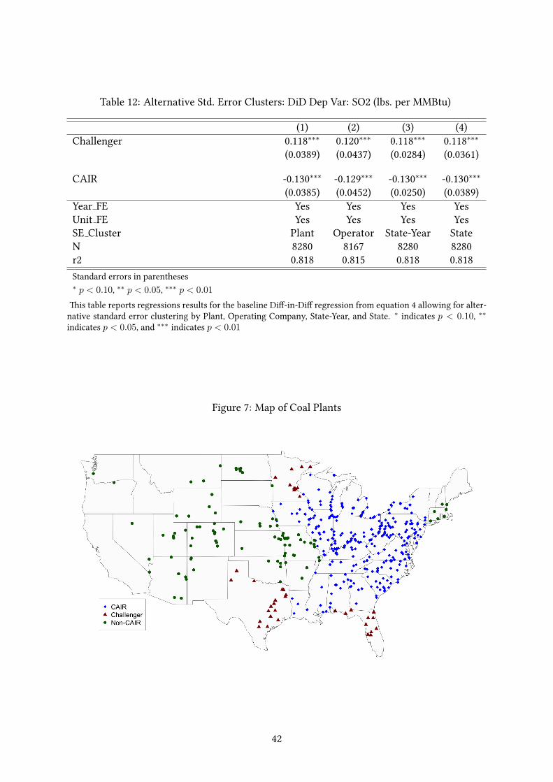
Table 12: Alternative Std. Error Clusters: DiD Dep Var: SO2 (lbs. per MMBtu)

(1) (2) (3) (4)

Challenger 0.118∗∗∗

0.120∗∗∗

0.118∗∗∗

0.118∗∗∗

(0.0389) (0.0437) (0.0284) (0.0361)

CAIR -0.130∗∗∗

-0.129∗∗∗

-0.130∗∗∗

-0.130∗∗∗

(0.0385) (0.0452) (0.0250) (0.0389)

Year FE Yes Yes Yes Yes

Unit FE Yes Yes Yes Yes

SE Cluster Plant Operator State-Year State

N 8280 8167 8280 8280

r2 0.818 0.815 0.818 0.818

Standard errors in parentheses

∗ p < 0.10,∗∗ p < 0.05,

∗∗∗ p < 0.01

�is table reports regressions results for the baseline Di�-in-Di� regression from equation 4 allowing for alter-

native standard error clustering by Plant, Operating Company, State-Year, and State.∗

indicates p < 0.10,∗∗

indicates p < 0.05, and∗∗∗

indicates p < 0.01

Figure 7: Map of Coal Plants

42

Figure 8: Marginal Kernel Density Plots for Observed Covariates

43

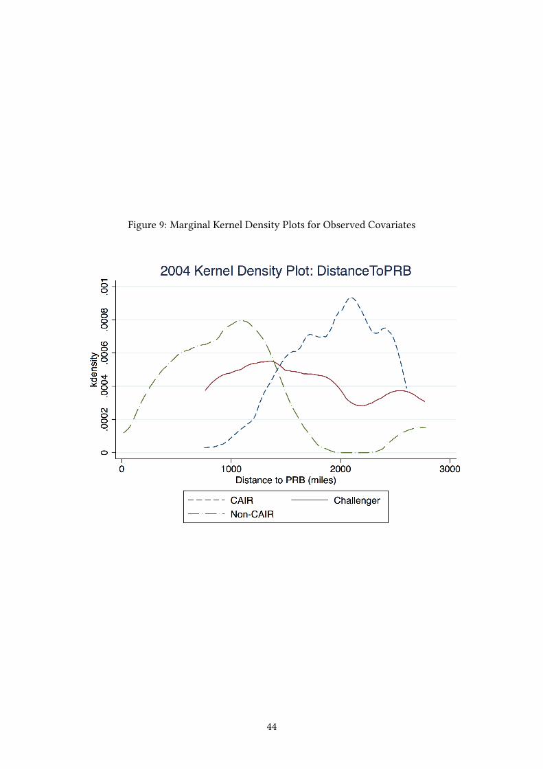
Figure 9: Marginal Kernel Density Plots for Observed Covariates

44