volatility and causality in strategic commodities
TRANSCRIPT

International Journal of Economics and Finance; Vol. 9, No. 8; 2017
ISSN 1916-971X E-ISSN 1916-9728
Published by Canadian Center of Science and Education
162
Volatility and Causality in Strategic Commodities: Characteristics,
Myth and Evidence
Youngho Chang1, Zheng Fang
1 & Shigeyuki Hamori
2
1 School of Business, Singapore University of Social Sciences, Singapore
2 Graduate School of Economics, Kobe University, Japan
Correspondence: Zheng Fang, School of Business, Singapore University of Social Sciences, 461 Clementi Road,
Singapore. Tel: 65-6248-0314. E-mail: [email protected]
Received: May 23, 2017 Accepted: June 22, 2017 Online Published: July 20, 2017
doi:10.5539/ijef.v9n8p162 URL: https://doi.org/10.5539/ijef.v9n8p162
Abstract
Commodity prices have fluctuated sharply and Brent oil has been considered the most volatile commodity in
price. This paper aims to reveal the true characteristics of the price volatility of six commodities, namely, Brent
oil, gold, silver, wheat, corn and soybean and to verify the existence of a long-run relationship and causation
among each pair of commodity prices. It finds that there has been persistent volatility in prices of all six
commodities from 1986 to 2010. Contrary to the common belief, however, Brent oil appears not to be the most
volatile in price. Rather the prices of precious metals and agricultural commodities have been more volatile than
Brent oil for some time periods. It also finds that there has been a long-run relationship between the prices of
Brent oil and soybean, of Brent oil and wheat, and a bilateral causality relationship between them, which implies
that there has been a simultaneous impact on the price trajectories of these commodities.
Keywords: GARCH, asymmetry, news impact curve, cointegration, Granger-causality
1. Introduction
The volatility of oil price has been increasingly gaining attention in both theory and practice. One of the reasons
is that crude oil is one of the most traded commodities in the world, and its price is supposedly the most volatile
in the market (Regnier, 2007; Verleger, 1993) (Note 1). The dynamics of oil prices have vast impacts on the
economy. Since energy commodities are key inputs to a plethora of economic activities, higher crude oil prices
will more often than not lead to higher production cost and therefore higher prices of final goods. It will exert
significant upward pressure on the consumer price index (CPI) and the result will be a negative impact on
economic growth (Jimenez-Rodriguez & Sanchez, 2005). Therefore, frequent and large magnitude fluctuating oil
prices can affect the businesses in any country (both oil-importing and oil-exporting), especially when there is an
increasing reliance on oil.
While there is a growing number of studies focusing on trends and volatility behavior of energy commodity
prices (for instance, Sadorsky, 2006; Narayan & Narayan, 2007; Wei et al., 2010; Arouri et al., 2012; Salisu&
Fasanya, 2013), the dynamics of non-oil commodity prices cannot be ignored as well. Take agricultural
commodities as an example. On the macroeconomic level, volatility of agricultural commodity prices may have
negative impact on growth and poverty and they are very damaging to the poor countries (Ramey & Ramey,
1995; Rodrick, 1999). On the microeconomic level, volatility may also impact decisions of farmers and
governments. A downward fluctuation would be adverse for farmers, but for a consumer, the reverse is true.
Besides, a comparison of the volatility of crude oil prices against three other major groups of commodities,
namely, precious metals and agricultural goods, using daily prices is relatively under-explored. The question how
oil price volatility compares with price volatility of other commodities is important because the conventional
wisdom that crude oil prices are more volatile ever since the oil crisis in 1973 may not stand up to rigorous
analysis. If oil price volatility is more severe compared to prices of other commodities, the oil industry is likely
to design some special treatments to handle risk and uncertainties. They may find vertical integration that avoids
transaction cost more attractive. Or, they may tend to rely more heavily on hedging and long-term contracts. If
otherwise, oil price risk may not deserve special attention.
This paper aims to study the price and volatility behavior of three types of strategic commodities using daily
ijef.ccsenet.org International Journal of Economics and Finance Vol. 9, No. 8; 2017
163
series covering a period of 1986-2010. First, we will examine whether price shocks have persistent and
asymmetric effects on volatility. Following that, we will study whether the conventional wisdom is true across
the whole time period examined. Finally, we will look into any correlation or Granger causality relationships
between the commodities.
The remainder of this paper is organized as follows. Section 2 reviews the pricing mechanisms and markets of
the six commodities. Section 3 critically reviews the related literature on volatility of commodity prices while
Section 4 describes the data and methodologies used to model volatility, cointegration and causation amongst the
different sub categories of commodities. Section 5 presents the results and Section 6 concludes this study with
policy implications.
2. Background
As proposed by Plourde and Watkins (1998), comparisons of price volatility across different commodities must
heed basic industry pricing mechanisms and market structures. This section reviews pricing mechanisms and
markets of the commodities examined in this paper.
The fundamentals of crude oil pricing have transformed radically since 1970s. Prior to 1970s, crude oil price was
around US$3.5 per barrel and prices were determined largely by the big oil companies. This arrangement
changed after the first world oil shock in October 1973 when the Organization of Arab Petroleum Exporting
Countries (OAPEC (Note 2)) proclaimed an oil embargo because of the Yom Kippur War (Note 3). During this
time, the Organization of Petroleum Exporting Countries (OPEC) was the price setter until early 1980s when
market forces began to take over the determination of oil prices. Compounded by the Iraq-Iran conflict, oil prices
had spiked up to US$30 per barrel by 1981. 1983 was a milestone in crude oil price determination as it marks the
introduction of New York Mercantile Exchange (NYMEX) of crude oil futures contract trading. Since then,
copious market instruments have surfaced to facilitate risk management associated to crude oil price changes.
Paradoxically, oil market participants had witnessed a phenomenon of „volatile‟ oil prices with the increased
reliance on the market mechanisms.
Gold has a long history as currency, reserves and an investment tool. In the 19th
century, many European
countries implemented the gold standard. After World War II, the United States dollar is pegged to gold at a rate
of US$35 per troy ounce under the Bretton Woods System. The system only ceased after the Nixon Shock in
1971 when the US unilaterally suspended the fungible system between gold and the greenback. In recent times,
gold has one of the most popular entities used as investment among all the precious metals. Not only that, gold
can be used to hedge or harbor against economic, political or currency crisis. This is because gold is an
investment asset which is commonly known as the “safe haven”, an asset that investors park their money during
financial crisis. Gold trading is done over-the-counter (OTC) and the largest global centre for clearing OTC
transactions for gold is London Bullion Market (LBM). Like most commodities, the gold market is subjected to
speculation through the use of market instruments such as derivatives. Investors in advanced and emerging
markets often switch between oil and gold or combine them to diversify their portfolios (Soytas et al., 2009).
Monetary authorities throughout the world pay close attention to gold prices to determine if their monetary
policies are on course (Le & Chang, 2012). The conventional wisdom is that gold has had low correlation with
other commodity prices and it is of our interest to prove it.
Silver, on the other hand, is similar to gold in the sense that it also has a long history as currency, reserves and an
investment tool. Since the end of the silver standard, however, silver has lost its role as a legal tender in many
developed countries. Like gold, silver is traded largely in the LBM but the silver market is smaller than gold.
Agricultural commodity price volatility has been growing concern for many years now. Prior to the global
financial crisis, an unprecedented global commodity boom took the world by storm. The boom, also known as
the “commodity supercycle”, saw the real price of food commodities increased by seventy-five per cent over five
years, from 2003 to 2008 (Erten & Ocampo, 2013). The U.S Drought 2012, which is one of the most severe and
extensive drought in 25 years, also had adverse impacts on crop and livestock sectors. The result was higher
agricultural prices. All these underlined the needs for policymakers as well as farmers to better understand the
volatility of agricultural price in a bid to lower the risks faced by many stakeholders. In 2009, the Organization
for Economic Co-operation and Development (OECD) highlighted that the agricultural market remains
unprotected to the following risks: institutional, market, financial and personal risks. Out of these risks, market
risk remains as one of the most salient as it encompasses a lot of the uncertainties farmers will obtain for their
products to pay for their inputs.

ijef.ccsenet.org International Journal of Economics and Finance Vol. 9, No. 8; 2017
164
3. Literature Review
There is a large amount of literature on the price volatility of individual commodities and associated volatility
characteristics. Some non-comparative literature include Narayan and Narayan (2007), Kuper (2002) and Gileva
(2010) who have attempted to model oil price volatility using parametric methods such as GARCH and
EGARCH. They seem to have come to different conclusions on the asymmetry of effects that shocks have on the
volatility of crude oil ranging from a total absence of asymmetry to a clear indication of asymmetry. Other
literature focusing on volatility modeling of other commodities such as agricultural commodities have also been
done using similar parametric methods and have come to the conclusion that the median volatility of these
agricultural commodity groups have not increased nor decreased from 1957-2001 (Moledina, Roe, & Shane,
2004).
In contrast, comparative studies on volatility modeling are also abundant with a variety of different parametric
and non-parametric methods. The non-parametric approach was adopted by Plourde and Watkins (1998), Regnier
(2007) and Calvo-Gonzalez, Shankar and Trezzi (2010) where the first two studies concluded that generally
crude oil prices were more volatile as compared to a variety of other commodities while Gonzalez, Shankar and
Trezzi (2010) argued that there has been no upward or downward trend in volatility over time.
Studies by Narayan and Liu (2011), Clem (1985) and Jacks, O‟Rourke and Williamson (2009), however, adopted
parametric approaches. The study done by Narayan and Liu (2011) is the closest to ours, as the bundle of
commodities being compared contains both gold and silver which are also being studied in this paper. The latter
two studies focused on examining the volatility of oil with respect to non-crude oil material.
Additionally, comparative studies on the correlation and causality relationships between commodity prices have
also been done using standard methods such as the Johansen cointegration test, VAR and VECM models. For
example, Saghaian (2010) evaluated the correlation and causality relationships between crude oil, ethanol and a
variety of agricultural commodities using the VECM model, and concluded that although there may be
correlation between oil and other commodities, there is mixed evidence of causality between commodities.
Another paper by Le and Chang (2011), focusing on the relationship between oil and gold, have instead found a
long-run relationship between the two commodities after testing for correlation and causality. Le and Chang
(2016) explored dynamics between strategic commodities and found that oil prices seem to not give any
information about price fluctuations of financial variables such as interest rate, exchange rate or stock prices in
the long run but some information about volatility of those variables in the short run.
Even though studies of energy, metals, agriculture commodities, or a combination of either two groups are
aplenty, there seems to be no studies examining these three commodity classes altogether with the application of
parametric methods such as GARCH to model volatility.
4. Data and Methods
4.1 Data
For this study, daily price series of Brent crude oil, gold, silver, wheat, corn and soybean covering the period
between 01 January 1986 and 31 December 2010 are employed (Note 4). The data for precious metals of gold
and silver reflect LBM prices. The data for wheat, corn and soybean were sourced from the U.S. Department of
Agriculture (USDA) while Brent (current month f.o.b.) price series were sourced from Independent Chemical
Information Service (ICIS) Pricing. The data on all series are compiled from DataStream. In total, there are
39,138 daily prices (six commodities *6523 daily prices) and the sample period will be divided every five years
to form five sub-sample periods: 1986/1990, 1991/1995, 1996/2000, 2001/2005 and 2006/2010.
The return is calculated as the logarithm of price at the present period less the logarithm of price at the last
period. Table 1 shows the descriptive statistics for prices and returns of all the six commodities for the whole
period of 1986-2010. The Jarque-Bera test statistics suggest that neither prices nor returns are normally
distributed. Therefore, when modeling volatility using return series, one could either use a non-normal
distribution such as the Student-𝑡 distribution (or that with fixed degree of freedom) and the generalized error
distribution (or that with fixed parameter), or use robust standard errors by selecting Bollerslev-Wooldridge
heteroskedasticity consistent covariance matrix. This paper adopts the second alternative so as to obtain valid
inferences. In addition, the kurtosis greater than three implies the series has a fat tail. For the price series, the
positive skewness indicates the presence of a right tail; and for the return series, there is evidence of a left tail.
The right tail of prices and left tail of returns are also found in Salisu and Fasanya (2013). Furthermore, the
standard deviation of return series seems to suggest that Brent is the most volatile among the six. But whether it
is always more volatile across the whole time span is worthy of more investigation.

ijef.ccsenet.org International Journal of Economics and Finance Vol. 9, No. 8; 2017
165
Table 1. Descriptive statistics for prices and returns
Brent Gold Silver Wheat Soybean Corn
Panel A: Prices
Mean 33.15 463.91 7.22 3.66 6.62 2.55
Median 20.80 383.40 5.31 3.45 5.89 2.33
Maximum 145.61 1417.85 30.70 11.95 16.19 7.08
Minimum 8.75 252.85 3.55 1.92 3.88 1.22
Std. dev. 24.65 235.04 4.34 1.21 2.03 0.87
Skewness 1.67 2.04 2.07 2.09 1.61 1.76
Kurtosis 5.31 6.51 7.30 9.23 5.64 6.75
Jarque-Bera 4472 7865 9714 15290 4699 7192
Observations 6523 6523 6523 6523 6523 6523
Panel B: Returns
Mean 0.0002 0.0002 0.0003 0.0001 0.0001 0.0001
Median 0.0000 0.0000 0.0000 0.0000 0.0000 0.0000
Maximum 0.1942 0.0738 0.1828 0.2258 0.0745 0.0947
Minimum -0.4387 -0.0722 -0.1608 -0.2295 -0.1673 -0.1258
Std. dev. 0.0248 0.0096 0.0181 0.0220 0.0152 0.0182
Skewness -0.8915 -0.1728 -0.1940 -0.4863 -0.7669 -0.3749
Kurtosis 25.1075 10.2134 10.9787 15.0404 10.0986 7.7621
Jarque-Bera 133680 14172 17341 39653 14333 6315
Observations 6522 6522 6522 6522 6522 6522
The dynamics of prices and returns of Brent oil, Gold, Silver, Wheat, Soybean and Corn is plotted in Figure 1. It
is obvious that (1) the volatility of the series is not constant over time; (2) return series show evidence of
volatility clustering in the sense that periods of high returns are followed by periods of high returns, and periods
of small returns are followed by periods of small returns; (3) some of the series seem to exhibit breaks,
particularly around the time the financial crisis to be broke out (Note 5).
Table 2 shows the unit root test results for the returns both in the whole sample and in five sub-sample periods.
The augmented Dickey-Fuller, or ADF (Dickey and Fuller, 1981) test is employed on the return series with
intercept only. The results show that the null hypothesis of existence of a unit root is significantly rejected at the
conventional levels of significance, suggesting stationarity of return series. The stationarity of returns are also
supported by other unit root tests such as Phillips-Perron (PP) test (Phillips & Perron, 1988) and
Kwiatkowski-Philips-Schmidt-Shin (KPSS) test (Kwiatkowski et al., 1992). Furthermore, ARCH test statistics
reject the “no ARCH” hypothesis for all the six return series (Note 6). Due to space limitation, these results are
not reported but available from authors upon request. Based on the above pre-estimation analysis, it is
appropriate to model the volatility via GARCH models.
0
40
80
120
160
-.6
-.4
-.2
.0
.2
86 88 90 92 94 96 98 00 02 04 06 08 10
Brent price Brent return
0
400
800
1,200
1,600
-.08
-.04
.00
.04
.08
86 88 90 92 94 96 98 00 02 04 06 08 10
Gold price Gold return
0
5
10
15
20
25
30
35
-.2
-.1
.0
.1
.2
86 88 90 92 94 96 98 00 02 04 06 08 10
Silver price Silver return
0
2
4
6
8
10
12
14
-.3
-.2
-.1
.0
.1
.2
.3
86 88 90 92 94 96 98 00 02 04 06 08 10
Wheat price Wheat return
0
4
8
12
16
20
-.20
-.15
-.10
-.05
.00
.05
.10
86 88 90 92 94 96 98 00 02 04 06 08 10
Soybean price Soybean return
0
2
4
6
8
-.15
-.10
-.05
.00
.05
.10
86 88 90 92 94 96 98 00 02 04 06 08 10
Corn price Corn return

ijef.ccsenet.org International Journal of Economics and Finance Vol. 9, No. 8; 2017
166
0
40
80
120
160
-.6
-.4
-.2
.0
.2
86 88 90 92 94 96 98 00 02 04 06 08 10
Brent price Brent return
0
400
800
1,200
1,600
-.08
-.04
.00
.04
.08
86 88 90 92 94 96 98 00 02 04 06 08 10
Gold price Gold return
0
5
10
15
20
25
30
35
-.2
-.1
.0
.1
.2
86 88 90 92 94 96 98 00 02 04 06 08 10
Silver price Silver return
0
2
4
6
8
10
12
14
-.3
-.2
-.1
.0
.1
.2
.3
86 88 90 92 94 96 98 00 02 04 06 08 10
Wheat price Wheat return
0
4
8
12
16
20
-.20
-.15
-.10
-.05
.00
.05
.10
86 88 90 92 94 96 98 00 02 04 06 08 10
Soybean price Soybean return
0
2
4
6
8
-.15
-.10
-.05
.00
.05
.10
86 88 90 92 94 96 98 00 02 04 06 08 10
Corn price Corn return
Figure 1. Plots of prices and returns for the period 1986-2010
Table 2. ADF-unit root test results for the returns
Brent Gold Silver Wheat Soybean Corn
Full sample -81.505 -81.552 -88.687 -86.452 -83.132 -80.334
1986-1990 -37.294 -37.826 -41.737 -38.059 -37.743 -35.327
1991-1995 -25.194 -37.233 -39.789 -38.839 -37.396 -37.505
1996-2000 -36.144 -34.447 -42.465 -35.262 -35.881 -34.801
2001-2005 -38.073 -36..424 -37.195 -38.371 -38.376 -37.606
2006-2010 -35.478 -36.428 -38.573 -40.038 -36.495 -35.680
Note. The test is based on the level data with only intercepts and no time trends in the model. In the table are t-statistics of ADF-unit root test.
As shown, all statistics are rejected at the 1% significance level, indicating no unit root in the return series.
4.2 Econometric models
4.2.1 Modeling Volatility
GARCH models (Engle, 1982; Bollerslev, 1986) are employed when the error term shows conditional
heteroskedasticity. Let the error process be such that
𝜀𝑡 = 𝑣𝑡√ℎ𝑡 , (1)
where*𝑣𝑡+ is a white-noise process with 𝜍𝑣2 = 1 and
ℎ𝑡 = 𝑎0 + ∑ 𝑎𝑖𝜀𝑡−𝑖2𝑞
𝑖=1 + ∑ 𝑏𝑗ℎ𝑡−𝑗𝑝𝑗=1 , (2)
The conditional variance of 𝜀𝑡 is given by 𝐸𝑡−1𝜀𝑡2 = ℎ𝑡, which is an 𝐴𝑅𝑀𝐴 process. This is known as the
generalized 𝐴𝑅𝐶𝐻 or 𝐺𝐴𝑅𝐶𝐻(𝑝, 𝑞) model. Usually it is adequate to obtain a good model fit for stationary
financial time series with ARCH effects using a 𝐺𝐴𝑅𝐶𝐻(1,1) model with only three parameters in the
conditional variance equation. Indeed, Hanes and Lunde (2004) provided compelling evidence that it is difficult
to find a volatility model that outperforms the simple GARCH(1,1).
The GARCH(1,1) shows mean reversion to a constant for all time. When the mean reverts to a varying level, the
ijef.ccsenet.org International Journal of Economics and Finance Vol. 9, No. 8; 2017
167
Component 𝐺𝐴𝑅𝐶𝐻 (𝐶𝐺𝐴𝑅𝐶𝐻) is appropriate. The 𝐶𝐺𝐴𝑅𝐶𝐻(1,1) model is as follows:
ℎ𝑡 − 𝑚𝑡 = 𝑎1(𝜀𝑡−12 − 𝑚𝑡−1) + 𝑏1(ℎ𝑡−1 − 𝑚𝑡−1), (3)
𝑚𝑡 = 𝑐 + 𝜌(𝑚𝑡−1 − 𝑐) + 𝜙(𝜀𝑡−12 − ℎ𝑡−1), (4)
Where 𝑚𝑡 is the time varying long-run volatility. Equations (3) and (4) describe transitory and permanent
components, respectively. The transitory component, ℎ𝑡 − 𝑚𝑡, converges to zero with powers of 𝑎1 + 𝑏1, while
the permanent component 𝑚𝑡 converges very slowly to 𝑐 with powers of 𝜌, which is typically near to 1.
Both 𝐺𝐴𝑅𝐶𝐻 and 𝐶𝐺𝐴𝑅𝐶𝐻 are used to account for symmetric volatility effects. It is widely known, however,
that empirically bad news (negative shocks) or good news (positive shocks) induce asymmetric or leverage
effects on the conditional volatility of most financial assets. Consequently, the 𝐺𝐴𝑅𝐶𝐻(1,1) and 𝐶𝐺𝐴𝑅𝐶𝐻(1,1)
models would not be suitable and we will next consider two different asymmetric volatility models when there
are the leverage effects.
The first one is the exponential 𝐺𝐴𝑅𝐶𝐻 (𝐸𝐺𝐴𝑅𝐶𝐻) model proposed by Nelson (1991). The 𝐸𝐺𝐴𝑅𝐶𝐻(1,1) is
specified as follows:
ln(ℎ𝑡) = 𝑎0 + 𝑎1|𝜀𝑡−𝑖|
√ℎ𝑡−𝑖+ 𝜆1
𝜀𝑡−1
√ℎ𝑡−1+ 𝑏1ln (ℎ𝑡−1) (5)
Note that when 𝜀𝑡−1 is positive or there is “good news”, the effect of standardized value of 𝜀𝑡−1(𝑖. 𝑒. ,𝜀𝑡−1
√ℎ𝑡−1) on
the log of the conditional variance is (𝑎1 + 𝜆1); in contrast, when 𝜀𝑡−1 is negative or there is “bad news”, the
effect of standardized value of 𝜀𝑡−1 is (𝑎1 − 𝜆1). Bad news can have a larger impact on volatility when the
value of 𝜆1is negative. An advantage of the 𝐸𝐺𝐴𝑅𝐶𝐻 model over the basic 𝐺𝐴𝑅𝐶𝐻 model is that the
conditional variance ℎ𝑡 is guaranteed to be positive regardless of the values of the coefficients in (5), because
the logarithm of ℎ𝑡 instead of ℎ𝑡 itself is modeled.
The second 𝐺𝐴𝑅𝐶𝐻variant that is capable of modeling leverage effects is the threshold 𝐺𝐴𝑅𝐶𝐻 (𝑇𝐺𝐴𝑅𝐶𝐻)
model proposed by Glosten, Jagannathan, Runkle (1994) (Note 7). The 𝑇𝐺𝐴𝑅𝐶𝐻(1,1) has the following form
ℎ𝑡 = 𝑎0 + 𝑎1𝜀𝑡−12 + 𝜆1𝑆𝑡−1𝜀𝑡−1
2 + 𝑏1ℎ𝑡−1 (6)
where
𝑆𝑡−1 = {1 if 𝜀𝑡−1 < 00 if𝜀𝑡−1 ≥ 0
That is, depending on whether 𝜀𝑡−1 is above or below the threshold value of zero, an 𝜀𝑡−1 shock has different
effects on the conditional varianceℎ𝑡. When 𝜀𝑡−1 is positive, the total effects are given by 𝑎1𝜀𝑡−12 ; when 𝜀𝑡−1
is negative, the total effects are given by (𝑎1 + 𝜆1)𝜀𝑡−12 . Therefore, one would expect 𝜆1 to be positive for bad
news having larger impacts.
To clearly see the leverage effects in these models, Pagan and Schwert (1990) and Engle and Ng (1993)
advocated the use of news impact curve. They defined the news impact curve as the functional relationship
between conditional variance at time tand the shock term (error term) at time t − 1, holding constant the
information dated t − 2 and earlier, and with all lagged conditional variance evaluated at the level of the
unconditional variance. Therefore, the equation for the 𝐸𝐺𝐴𝑅𝐶𝐻(1,1) news impact curve is:
ℎ𝑡 = 𝐴exp*(𝑎1|𝜀𝑡−1| + 𝜆1𝜀𝑡−1)/𝜍+ , (7)
where 𝐴 = 𝜍2𝑏1exp*𝑎0+, and 𝜍2 = exp{(𝑎0 + 𝑎1√2/𝜋)/(1 − 𝑏1)}
The equation for the 𝑇𝐺𝐴𝑅𝐶𝐻(1,1) news impact curve is:
ℎ𝑡 = 𝐴 + (𝑎1 + 𝜆1𝑆𝑡−1) 𝜀𝑡−12 (8)
where 𝐴 = 𝑎0 + 𝑏1𝜍2, and 𝜍2 = 𝑎0/,1 − (𝑎1 +𝜆1
2) − 𝑏1-.
4.2.2 Engle-Granger Two-Step Error Correction Model
To examine the cointegration and causality between two variables, we adopt the Engle-Granger two-step error
correction model. The first step is to conduct the Engle-Granger cointegration test, which is preferable to
Johansen cointegration test (Johansen & Juselius, 1990) because we are only interested in the bivariate
relationship instead of cointegration within a multivariate framework. Both variables have to be integrated of the
ijef.ccsenet.org International Journal of Economics and Finance Vol. 9, No. 8; 2017
168
same order before checking for any possible cointegration. When both variables are integrated of the same order,
say I(1), using methods suggested by Engle and Granger (1987), one can first regress one I(1) variable on
another using ordinary least squares:
𝑌𝑡 = 𝛼 + 𝛽𝑍𝑡 + 𝜀𝑡 (9)
The estimated residuals are then tested for non-stationarity using the ADF and PP tests using optimal lags
suggested by Akaike information criterion (AIC) and Schwarz information criterion (SIC) tests. The null
hypothesis is that the residuals are non-stationary and rejection of the null hypothesis leads to the conclusion that
the residuals are stationary and the series are cointegrated. If the two non-stationary time series variables are
cointegrated and have a long-run relationship, they are expected to move together through time. However, if the
variables are integrated of different orders, it can be concluded that they are not cointegrated.
A conintegrating relationship implies the existence of causality in at least one direction. Upon establishing a
cointegrating relationship and obtaining an estimate of residuals, the second step is to identify the direction of
Granger causality through an Error Correction Model (ECM). All the variables in this model have to be
stationary. The basic structure of the ECM is as follows:
∆𝑌𝑡 = 𝛼1 + 𝛽1𝐸𝐶𝑡−1 + ∑ 𝑎11(𝑖)∆𝑌𝑡−𝑖𝑖=1 + ∑ 𝑎12(𝑖)∆𝑍𝑡−𝑖𝑖=1 + 𝜀𝑦𝑡 (10)
∆𝑍𝑡 = 𝛼2 + 𝛽2𝐸𝐶𝑡−1 + ∑ 𝑎21(𝑖)∆𝑌𝑡−𝑖𝑖=1 + ∑ 𝑎22(𝑖)∆𝑍𝑡−𝑖𝑖=1 + 𝜀𝑧𝑡 (11)
The EC component is derived from the cointegrated time series 𝐸𝐶𝑡 = 𝑌𝑡 − (𝛼 + 𝛽𝑋𝑡). The coefficient 𝛽1
captures the rate at which 𝑌 adjusts to the deviation from long-run equilibrium in the last period, and the
coefficient 𝛽2 captures the adjustment speed of the variable 𝑍 to its long-run equilibrium. Direct convergence
necessitates that 𝛽1 be negative and 𝛽2 be positive. If 𝛽1 = 0 and 𝑎12(𝑖) = 0, it can be said that the variable
𝑍 does not Granger cause 𝑌 in the long run. Similarly, if 𝛽2 = 0 and 𝑎21(𝑖) = 0, 𝑌 does not Granger cause
𝑍 in the long run.
5. Results and Discussion
5.1 Do Price Shocks have Asymmetric Effects on Volatility?
The volatility modelling procedures are summarized below:
Step 1: Analyze time series plot and descriptive statistics
Step 2: Generate stationary data by first differencing
Step 3: Return series and its ACF plots are checked for further confirmation of stationarity
Step 4: Since squared returns measure the second order moment of the commodity‟s time series, its ACF is
plotted to check for autocorrelation.
Step 5: Ljung-Box and ARCH LM tests with 5% significance level with 10, 20 and 30 lags are conducted as
further confirmation. If autocorrelation and ARCH effects are rejected, time series do not exhibit time varying
conditional heteroskedasticity or volatility clustering; otherwise, time series exhibits time varying conditional
heteroskedasticity or volatility clustering.
Step 6: Return series is modelled using GARCH(1,1). Use AIC and SIC to select the best model across 5
different conditional densities for the innovations (i.e. Normal, Student‟s t, Generalized Error Distribution (GED),
Student‟s t with fixed degrees of freedom, and GED with fixed parameter); or, use robust standard errors
(Bollerslev-Wooldridge covariance matrix) for normal distribution.
Step 7: Conduct Sign Bias test (SB test) to determine if the time series exhibits symmetric volatility effects. If
the null hypothesis is rejected, model the volatility based on the 3 models (EGARCH(1,1), GJR-GARCH(1,1)
and APARCH(1,1,1)); and the final model is chosen based on BIC followed by model checks on the standardized
residuals to assess its suitability. If one fails to reject the null hypothesis, further model checks using Ljung-Box
and ARCH LM tests on the standardized residuals and Q-Q plot are utilized to assess model‟s suitability
Step 8: Indicate the persistence and leverage effect respectively. News impact curves is plotted to demonstrate
the effects of good and bad news have on the conditional volatility of the commodity.
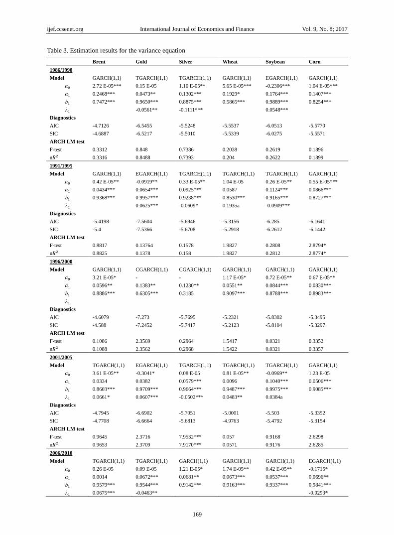
Following the procedures, we choose the model specifications for the returns of each commodity for each
sub-sample period. The model and corresponding estimation results for the variance equation are listed in Table
3.
ijef.ccsenet.org International Journal of Economics and Finance Vol. 9, No. 8; 2017
169
Table 3. Estimation results for the variance equation
Brent Gold Silver Wheat Soybean Corn
1986/1990
Model GARCH(1,1) TGARCH(1,1) TGARCH(1,1) GARCH(1,1) EGARCH(1,1) GARCH(1,1)
𝑎0 2.72 E-05*** 0.15 E-05 1.10 E-05** 5.65 E-05*** -0.2306*** 1.04 E-05***
𝑎1 0.2468*** 0.0473** 0.1302*** 0.1929* 0.1764*** 0.1407***
𝑏1 0.7472*** 0.9650*** 0.8875*** 0.5865*** 0.9889*** 0.8254***
𝜆1 -0.0561** -0.1111*** 0.0548***
Diagnostics
AIC -4.7126 -6.5455 -5.5248 -5.5537 -6.0513 -5.5770
SIC -4.6887 -6.5217 -5.5010 -5.5339 -6.0275 -5.5571
ARCH LM test
F-test 0.3312 0.848 0.7386 0.2038 0.2619 0.1896
n𝑅2 0.3316 0.8488 0.7393 0.204 0.2622 0.1899
1991/1995
Model GARCH(1,1) EGARCH(1,1) TGARCH(1,1) TGARCH(1,1) TGARCH(1,1) GARCH(1,1)
𝑎0 0.42 E-05** -0.0919** 0.33 E-05** 1.04 E-05 0.26 E-05** 0.55 E-05***
𝑎1 0.0434*** 0.0654*** 0.0925*** 0.0587 0.1124*** 0.0866***
𝑏1 0.9368*** 0.9957*** 0.9238*** 0.8530*** 0.9165*** 0.8727***
𝜆1 0.0625*** -0.0609* 0.1935a -0.0909***
Diagnostics
AIC -5.4198 -7.5604 -5.6946 -5.3156 -6.285 -6.1641
SIC -5.4 -7.5366 -5.6708 -5.2918 -6.2612 -6.1442
ARCH LM test
F-test 0.8817 0.13764 0.1578 1.9827 0.2808 2.8794*
n𝑅2 0.8825 0.1378 0.158 1.9827 0.2812 2.8774*
1996/2000
Model GARCH(1,1) CGARCH(1,1) CGARCH(1,1) GARCH(1,1) GARCH(1,1) GARCH(1,1)
𝑎0 3.21 E-05* - - 1.17 E-05* 0.72 E-05** 0.67 E-05**
𝑎1 0.0596** 0.1383** 0.1230** 0.0551** 0.0844*** 0.0830***
𝑏1 0.8886*** 0.6305*** 0.3185 0.9097*** 0.8788*** 0.8983***
𝜆1
Diagnostics
AIC -4.6079 -7.273 -5.7695 -5.2321 -5.8302 -5.3495
SIC -4.588 -7.2452 -5.7417 -5.2123 -5.8104 -5.3297
ARCH LM test
F-test 0.1086 2.3569 0.2964 1.5417 0.0321 0.3352
n𝑅2 0.1088 2.3562 0.2968 1.5422 0.0321 0.3357
2001/2005
Model TGARCH(1,1) EGARCH(1,1) TGARCH(1,1) TGARCH(1,1) TGARCH(1,1) GARCH(1,1)
𝑎0 3.61 E-05** -0.3041* 0.08 E-05 0.81 E-05** -0.0969** 1.23 E-05
𝑎1 0.0334 0.0382 0.0579*** 0.0096 0.1040*** 0.0506***
𝑏1 0.8603*** 0.9709*** 0.9664*** 0.9487*** 0.9975*** 0.9085***
𝜆1 0.0661* 0.0607*** -0.0502*** 0.0483** 0.0384a
Diagnostics
AIC -4.7945 -6.6902 -5.7051 -5.0001 -5.503 -5.3352
SIC -4.7708 -6.6664 -5.6813 -4.9763 -5.4792 -5.3154
ARCH LM test
F-test 0.9645 2.3716 7.9532*** 0.057 0.9168 2.6298
n𝑅2 0.9653 2.3709 7.9170*** 0.0571 0.9176 2.6285
2006/2010
Model TGARCH(1,1) TGARCH(1,1) GARCH(1,1) GARCH(1,1) GARCH(1,1) EGARCH(1,1)
𝑎0 0.26 E-05 0.09 E-05 1.21 E-05* 1.74 E-05** 0.42 E-05** -0.1715*
𝑎1 0.0014 0.0672*** 0.0681** 0.0673*** 0.0537*** 0.0696**
𝑏1 0.9579*** 0.9544*** 0.9142*** 0.9163*** 0.9337*** 0.9841***
𝜆1 0.0675*** -0.0463** -0.0293*

ijef.ccsenet.org International Journal of Economics and Finance Vol. 9, No. 8; 2017
170
Diagnostics
AIC -4.9874 -5.8624 -4.6957 -4.1926 -5.3086 -4.6944
SIC -4.9636 -5.8386 -4.6758 -4.1728 -5.2888 -4.6706
ARCH LM test
F-test 0.9489 1.4106 0.2766 0.4415 0.1042 1.1026
n𝑅2 0.9497 1.4112 0.277 0.442 0.1043 1.1033
Note. ***, **, * and “a” represent significance levels at 1%, 5%, 10% and 15%, respectively. All models are based on AR(1) mean equation
with normal (robust) error distribution. The coefficient estimates on the time-varying long term variance in the CGARCH model are not
reported here.
In the 𝐺𝐴𝑅𝐶𝐻(1,1) models for Brent and Corn for the periods 1986-1990, 1991-1995, and 1996-2000, for
Wheat and Soybean during 1996-2000 and 2006-2010, for Corn during 2001-2005, and for Silver during
2006-2010, the sum of 𝐴𝑅𝐶𝐻 and 𝐺𝐴𝑅𝐶𝐻 effects is close to one, indicating shocks to volatility have a
persistent effect on the conditional variance (Note 8). While volatility of Wheat for the period of 1986-1990
follows 𝐺𝐴𝑅𝐶𝐻(1,1), the reversion to the mean is much quicker than other variance processes (the sum of
ARCH and GARCH effects is 0.78, much less than 1). Volatility of Gold and Silver for the period of 1996-2000
seems to be best fitted by 𝐶𝐺𝐴𝑅𝐶𝐻(1,1), which allows for mean reversion to a time varying long-run volatility.
The estimation for the long run component reveals that the time varying long-run volatility reverts very slowly
(the coefficient estimate is between 0.99 and 1). On the other hand, the transitory component shows that it
converges to zero with powers of 0.77 and 0.44 respectively (as indicated by 0.63+0.14 and 0.12+0.32).In sum,
price shocks have symmetric effect on the volatility of these markets.
For the rest, the volatility is best modeled using asymmetric 𝐺𝐴𝑅𝐶𝐻 models. The results of 𝑇𝐺𝐴𝑅𝐶𝐻 and
𝐸𝐺𝐴𝑅𝐶𝐻 models show evidence of leverage effects (as indicated by estimates of λ1) and therefore they are
chosen over the symmetric models. We anticipate that bad news (negative shocks) has the tendency to cause a
larger impact on volatility in most financial assets than good news (positive shocks) do. In the 𝑇𝐺𝐴𝑅𝐶𝐻 models,
the coefficient measuring the leverage effect is positive for Wheat during 1991-1995, for Brent, Wheat and
Soybean during 2001-2005, and for Brent during 2006-2010, indicating that bad news have a larger impact on
price volatility than good news in these markets, while the coefficient is negative for Gold and Silver for the
periods 1986-1990, Silver and Soybean for 1991-1995, Silver for 2001-2005and Gold for 2006-2010, suggesting
that good news have a larger impact for markets at the specific time period. In the 𝐸𝐺𝐴𝑅𝐶𝐻 models, a positive
coefficient of λ1 indicates good shocks affecting volatility more than bad shocks, and vice versa. As such, the
market of Soybean in late 1980s, Gold in the first half of 1990s and 2000s are found to be affected more by
positive shocks than negative shocks, while in the Corn market for 2006-2010, bad news has a larger impact on
the volatility.
Next to the estimation results, the diagnostic statistics of AIC and SIC, which are used for the selection of
volatility model specifications are reported. The post-estimation 𝐴𝑅𝐶𝐻 tests (both the 𝐹-test and Chi-square
distributed 𝑛𝑅2 test) are carried out to ensure 𝐴𝑅𝐶𝐻 effects in the return series are well captured by the
GARCH model. As results show, the null hypothesis of “no 𝐴𝑅𝐶𝐻 effect” could not be rejected at the
conventional levels of significance.
Returns‟ volatility implied by the family of 𝐺𝐴𝑅𝐶𝐻 models has important implications for portfolio selection
and asset pricing. They serve as an important input to determine value of options and as volatility estimates for
dynamic hedging strategies. These concerns point to the need to have a correct understanding of the impact of
news on volatility. As discussed in the above section, we will use the news impact curve following Engle and Ng
(1993) who defined the news impact curve as follows:
The news impact curve is the functional relationship between conditional variance at time t and the
shock term (error term) at time t – 1, holding constant the information dated t – 2 and earlier, and with
all lagged conditional variance evaluated at the level of the unconditional variance.
Based on the model estimations in Table 3, we obtain the results of the presence and magnitude of the
asymmetric effects as summarized in Table 4. It is observed that the price volatility of Corn is quite symmetric in
early days, and it is not until the most recent five-year period (i.e., 2001-2005) it began to show asymmetric
volatility. Brent‟s volatility also became more asymmetric, while Gold price has shown asymmetric volatility
most of the time. Commodities‟ volatility and its implications deserve a study here as asymmetries in
commodities‟ volatility would inevitably affect the exchange rate and aggregate demand of an economy. It will
also have an impact on the commodities‟ investments of market participants. Wild price swings can cause huge
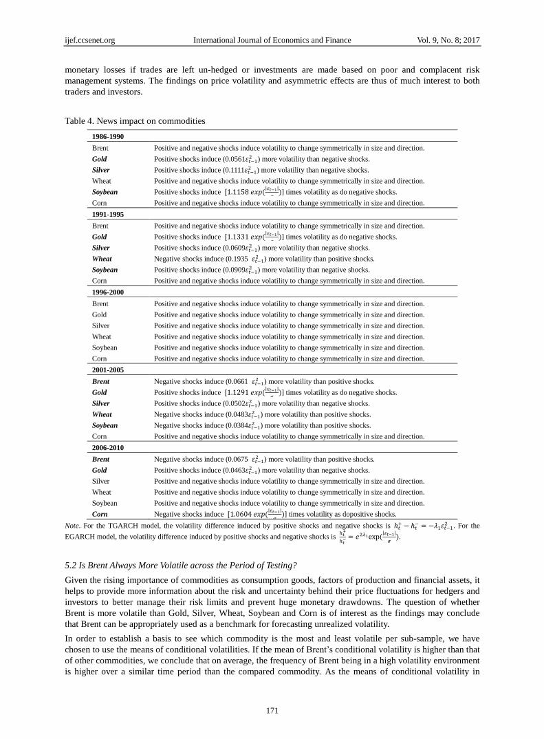
ijef.ccsenet.org International Journal of Economics and Finance Vol. 9, No. 8; 2017
171
monetary losses if trades are left un-hedged or investments are made based on poor and complacent risk
management systems. The findings on price volatility and asymmetric effects are thus of much interest to both
traders and investors.
Table 4. News impact on commodities
1986-1990
Brent Positive and negative shocks induce volatility to change symmetrically in size and direction.
Gold Positive shocks induce (0.0561𝜀𝑡−12 ) more volatility than negative shocks.
Silver Positive shocks induce (0.1111𝜀𝑡−12 ) more volatility than negative shocks.
Wheat Positive and negative shocks induce volatility to change symmetrically in size and direction.
Soybean Positive shocks induce ,1.1158 𝑒𝑥𝑝 (|𝜀𝑡−1|
𝜎)] times volatility as do negative shocks.
Corn Positive and negative shocks induce volatility to change symmetrically in size and direction.
1991-1995
Brent Positive and negative shocks induce volatility to change symmetrically in size and direction.
Gold Positive shocks induce ,1.1331 𝑒𝑥𝑝 (|𝜀𝑡−1|
𝜎)] times volatility as do negative shocks.
Silver Positive shocks induce (0.0609𝜀𝑡−12 ) more volatility than negative shocks.
Wheat Negative shocks induce (0.1935 𝜀𝑡−12 ) more volatility than positive shocks.
Soybean Positive shocks induce (0.0909𝜀𝑡−12 ) more volatility than negative shocks.
Corn Positive and negative shocks induce volatility to change symmetrically in size and direction.
1996-2000
Brent Positive and negative shocks induce volatility to change symmetrically in size and direction.
Gold Positive and negative shocks induce volatility to change symmetrically in size and direction.
Silver Positive and negative shocks induce volatility to change symmetrically in size and direction.
Wheat Positive and negative shocks induce volatility to change symmetrically in size and direction.
Soybean Positive and negative shocks induce volatility to change symmetrically in size and direction.
Corn Positive and negative shocks induce volatility to change symmetrically in size and direction.
2001-2005
Brent Negative shocks induce (0.0661 𝜀𝑡−12 ) more volatility than positive shocks.
Gold Positive shocks induce ,1.1291 𝑒𝑥𝑝 (|𝜀𝑡−1|
𝜎)] times volatility as do negative shocks.
Silver Positive shocks induce (0.0502𝜀𝑡−12 ) more volatility than negative shocks.
Wheat Negative shocks induce (0.0483𝜀𝑡−12 ) more volatility than positive shocks.
Soybean Negative shocks induce (0.0384𝜀𝑡−12 ) more volatility than positive shocks.
Corn Positive and negative shocks induce volatility to change symmetrically in size and direction.
2006-2010
Brent Negative shocks induce (0.0675 𝜀𝑡−12 ) more volatility than positive shocks.
Gold Positive shocks induce (0.0463𝜀𝑡−12 ) more volatility than negative shocks.
Silver Positive and negative shocks induce volatility to change symmetrically in size and direction.
Wheat Positive and negative shocks induce volatility to change symmetrically in size and direction.
Soybean Positive and negative shocks induce volatility to change symmetrically in size and direction.
Corn Negative shocks induce ,1.0604 𝑒𝑥𝑝 (|𝜀𝑡−1|
𝜎)] times volatility as dopositive shocks.
Note. For the TGARCH model, the volatility difference induced by positive shocks and negative shocks is ℎ𝑡+ − ℎ𝑡
− = −𝜆1𝜀𝑡−12 . For the
EGARCH model, the volatility difference induced by positive shocks and negative shocks is ℎ𝑡
+
ℎ𝑡− = 𝑒2𝜆1exp (
|𝜀𝑡−1|
𝜎).
5.2 Is Brent Always More Volatile across the Period of Testing?
Given the rising importance of commodities as consumption goods, factors of production and financial assets, it
helps to provide more information about the risk and uncertainty behind their price fluctuations for hedgers and
investors to better manage their risk limits and prevent huge monetary drawdowns. The question of whether
Brent is more volatile than Gold, Silver, Wheat, Soybean and Corn is of interest as the findings may conclude
that Brent can be appropriately used as a benchmark for forecasting unrealized volatility.
In order to establish a basis to see which commodity is the most and least volatile per sub-sample, we have
chosen to use the means of conditional volatilities. If the mean of Brent‟s conditional volatility is higher than that
of other commodities, we conclude that on average, the frequency of Brent being in a high volatility environment
is higher over a similar time period than the compared commodity. As the means of conditional volatility in

ijef.ccsenet.org International Journal of Economics and Finance Vol. 9, No. 8; 2017
172
Table 5 results show, over the five sub-samples, Brent is the most volatile commodity only in three periods –
1986/1990, 1996/2000 and 2001/2005. For the other two periods of 1991/1995 and 2006/2010, wheat is the most
volatile among the six strategic commodities. Meanwhile, it is interesting to note that gold is the least volatile
commodity for all the time. The comparison results of conditional volatility could be seen more
straightforwardly in Figure 2, where the scale of the y-axis is set the same. The findings do not provide evidence
to the proposition that Brent is more volatile than the five other strategic commodities in all sub-samples.
Table 5. Mean value of conditional volatility
Time Period Brent Gold Silver Wheat Soybean Corn
1986-1990 0.001160 0.000089 0.000294 0.000260 0.000197 0.000314
1991-1995 0.000418 0.000036 0.000240 0.000466 0.000130 0.000150
1996-2000 0.000607 0.000058 0.000242 0.000329 0.000191 0.000328
2001-2005 0.000512 0.000074 0.000252 0.000416 0.000280 0.000297
2006-2010 0.000504 0.000202 0.000623 0.001027 0.000342 0.000576
.000
.002
.004
.006
.008
.010
.012
.014
86 88 90 92 94 96 98 00 02 04 06 08 10
Conditional variance - Brent
.000
.002
.004
.006
.008
.010
.012
.014
86 88 90 92 94 96 98 00 02 04 06 08 10
Conditional variance - Gold
.000
.002
.004
.006
.008
.010
.012
.014
86 88 90 92 94 96 98 00 02 04 06 08 10
Conditional variance - Silver
.000
.002
.004
.006
.008
.010
.012
.014
86 88 90 92 94 96 98 00 02 04 06 08 10
Conditional variance - Wheat
.000
.002
.004
.006
.008
.010
.012
.014
86 88 90 92 94 96 98 00 02 04 06 08 10
Conditional variance - Soybean
.000
.002
.004
.006
.008
.010
.012
.014
86 88 90 92 94 96 98 00 02 04 06 08 10
Conditional variance - Corn
Figure 2. Conditional volatility

ijef.ccsenet.org International Journal of Economics and Finance Vol. 9, No. 8; 2017
173
5.3 Is There Correlation or Causality Between the Commodities?
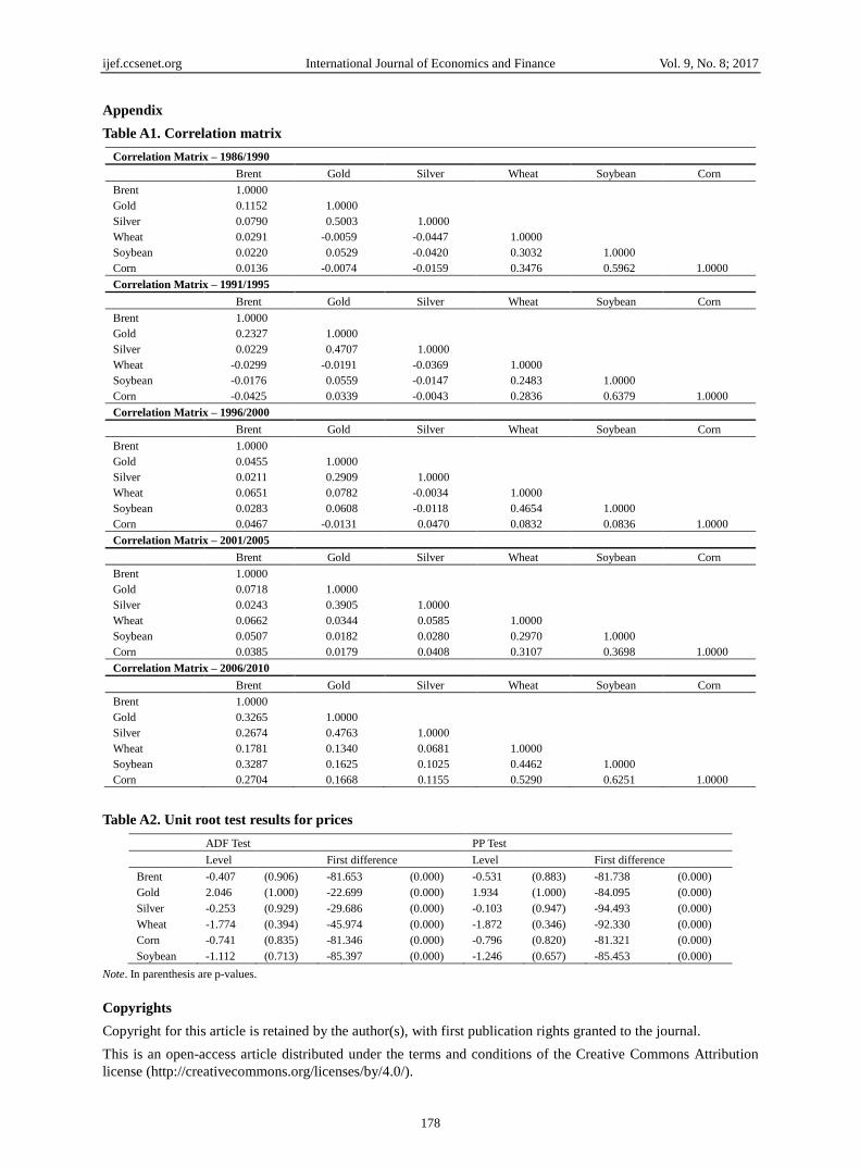
Based on the results of the correlation matrices among the six commodities' returns shown in Table A1, it is
found that across the 25 years, four pairs of commodities exhibited consistent high positive correlations. They
are gold and silver, wheat and corn, soybean and corn, and wheat and soybean. A noteworthy point from this
result was that in the last sub-sample period, correlation coefficients among all commodities exhibit strong
positive correlations and they have increased significantly compared to other periods. This could be due to the
incumbent highly integrated markets where hedge funds and traders trade all the commodities in the same basket.
Erten and Ocampo (2013) attributed the upswing in agricultural commodity prices during the commodity
super-cycle period to “extraordinary resilience of growth performance of major developing country demanders
of commodities, particularly China”. While many parties pushed the blame entirely to China‟s new consumption
pattern, there are also others who blamed it on other factors such as the weather, biofuel policies and speculators
etc. Unfortunately, empirical study in this area is scarce, and the underlying reasons behind the soaring
commodity prices require further in-depth study.
Table A2 shows the unit root tests results using ADF and PP tests on the level and the first difference of all the
price series for the entire sample period from 1986-2010. The SIC is employed for determining the optimal
number of lags. The period is not divided by every five years because the aim now is to detect and analyze the
possibility of a long run relationship. Should the analysis be broken up into sub-periods as was done with the
volatility modeling section, it may not yield enlightening results. Based on the unit root test results, it can be
established that at a significance level of 1%, all price series are non-stationary in level and integrated of the
same order, I(1). This is also consistent with the stationarity found in the return series.
Given the integrated series of the same order, we proceed to investigate the long-run relationship between all the
possible commodity pairs using the Engle-Granger cointegration test. As the nature of the relationship is only
bivariate and multiple cointegrating relationships are not of interest, this method is chosen above the Johansen
cointegration test (Johansen & Juselius, 1990). Table 6 summarizes the results and the numbers in bold indicate
the cointegrated commodity pairs. Cointegration between commodity pairs such as corn and wheat, soybean and
wheat, as well as soybean and corn are found and supported by prior research papers such as Arendarski and
Postek (2012). This phenomenon could be attributed partially to “herd behavior” where traders will be
alternatively bullish or bearish on all commodities for no plausible economic reason as they believe that
agricultural commodity prices tend to move together (Pindyck & Rotemberg, 1990). The weak cointegrating
relationships between Brent and Wheat, Brent and Soybean, and Gold and Soybean are also identified at the
significance level of 10%. However, a long-term equilibrium between gold and crude oil found by Le and Chang
(2011) and Zhang and Wei (2010) is not evident in our sample. Furthermore, the strong correlations between
gold and silver are found to not translate into the long-run relationship, which is consistent with Sari et al.
(2010).
Table 6. Engle-Granger cointegration results
t-statistic for lagged residuals
Gold Silver Wheat Corn Soybean
Brent -2.336 -1.678 -2.787* -2.550 -2.753*
Gold -2.466 -2.016 -2.306 -2.607*
Silver -1.717 -1.800 -1.777
Wheat -4.736*** -4.344***
Corn -4.257***
Note. ***, **, and * represent significance levels at 1%, 5%, and 10%, respectively.
Once cointegration relationships are established, the error correction model could be employed to test the
existence and direction of the short-run and long-run causality. The lag length is determined by the SIC in the
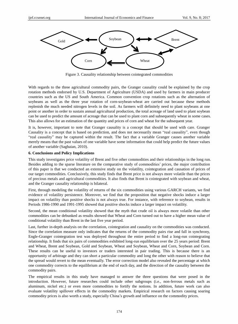
VAR model. The Granger causal relationships based on the Granger causality test results are summarized in
Figure 3. A short-run Granger causality running from Soybean to Wheat, Wheat to Corn, Soybean to Corn, and
Soybean to Gold is observed. A bi-directional Granger causal relationship between Wheat and Brent, and that
between Soybean and Brent also exist in the short-run. Next turn to the long-run causality, we find that the
short-run Granger causality also exists in the long run (Note 9).
ijef.ccsenet.org International Journal of Economics and Finance Vol. 9, No. 8; 2017
174
Figure 3. Causality relationship between cointegrated commodities
With regards to the three agricultural commodity pairs, the Granger causality could be explained by the crop
rotation methods endorsed by U.S. Department of Agriculture (USDA) and used by farmers in main producer
countries such as the US and South America. Common convention crop rotations such as the alternation of
soybeans as well as the three year rotation of corn-soybean-wheat are carried out because these methods
replenish the much needed nitrogen levels in the soil. As farmers will definitely need to plant soybeans at one
point or another in order to sustain annual agricultural production, the total acreage of land used to plant soybean
can be used to predict the amount of acreage that can be used to plant corn and subsequently wheat in some cases.
This also allows for an estimation of the quantity and prices of corn and wheat for the subsequent year.
It is, however, important to note that Granger causality is a concept that should be used with care. Granger
Causality is a concept that is based on prediction, and does not necessarily mean “real causality”, even though
“real causality” may be captured within the result. The fact that a variable Granger causes another variable
merely means that the past values of one variable have some information that could help predict the future values
of another variable (Saghaian, 2010).
6. Conclusions and Policy Implications
This study investigates price volatility of Brent and five other commodities and their relationships in the long run.
Besides adding to the sparse literature on the comparative study of commodities‟ prices, the major contribution
of this paper is that we conducted an extensive study on the volatility, cointegration and causation of prices of
our target commodities. Conclusively, this study finds that Brent price is not always more volatile than the prices
of precious metals and agricultural commodities. It also finds that Brent is cointegrated with soybean and wheat,
and the Granger causality relationship is bilateral.
First, through modeling the volatility of returns of the six commodities using various GARCH variants, we find
evidence of volatility persistence. Moreover, we find that the proposition that negative shocks induce a larger
impact on volatility than positive shocks is not always true. For instance, with reference to soybean, results in
Periods 1986-1990 and 1991-1995 showed that positive shocks induce a larger impact on volatility.
Second, the mean conditional volatility showed that the myth that crude oil is always more volatile than other
commodities can be debunked as results showed that Wheat and Corn turned out to have a higher mean value of
conditional volatility than Brent in the last five year period.
Last, further in-depth analysis on the correlation, cointegration and causality on the commodities was conducted.
Since the correlation measure only indicates that the returns of the commodity pairs rise and fall in synchrony,
Engle-Granger cointegration test was deployed throughout the entire period to find a long-run cointegrating
relationship. It finds that six pairs of commodities exhibited long-run equilibrium over the 25 years period: Brent
and Wheat, Brent and Soybean, Gold and Soybean, Wheat and Soybean, Wheat and Corn, Soybean and Corn.
These results can be useful to investors or traders interested in pair trading. This is because there is an
opportunity of arbitrage and they can short a particular commodity and long the other with reason to believe that
the spread would revert to the mean eventually. The error correction model also revealed the percentage at which
one commodity corrects to the equilibrium at the end of each day, and the direction of the causality between the
commodity pairs.
The empirical results in this study have managed to answer the three questions that were posed in the
introduction. However, future researches could include other subgroups (i.e., non-ferrous metals such as
aluminum, nickel etc.) or even more commodities to fortify the notions. In addition, future work can also
evaluate volatility spillover effects in the commodity markets. Empirical research on factors causing soaring
commodity prices is also worth a study, especially China‟s growth and influence on the commodity prices.
Corn Wheat
Soybean Brent Gold
ijef.ccsenet.org International Journal of Economics and Finance Vol. 9, No. 8; 2017
175
References
Agnolucci, P. (2009). Volatility in crude oil futures: A comparison of the predictive ability of GARCH and
implied volatility models. Energy Economics, 31(2), 316-321. https://doi.org/10.1016/j.eneco.2008.11.001
Arendarski, P., & Postek, L. (2012). Cointegration based trading strategy for soft commodities market. Working
Papers 2012-02, Faculty of Economic Sciences, University of Warsaw.
Bentzen, J. (2007). Does OPEC influence crude oil prices? Testing for co-movements and causality between
regional crude oil prices. Applied Economics, 39, 1375-1385. https://doi.org/10.1080/00036840600606344
Bollerslev, T. (1986). Generalized autoregressive conditional heteroskedasticity. Journal of Econometrics, 31,
307-327. https://doi.org/10.1016/0304-4076(86)90063-1
BP. (2012). Statistical Review of World Energy 2012. British Petroleum, London.
Calvo-González, O., Shankar, R., & Trezzi, R. (2010). Are commodity prices more volatile now? A Long-Run
Perspective (October 1, 2010). World Bank Policy Research Working Paper Series.
Cheong, C. W. (2009). Modeling and forecasting crude oil markets using ARCH-type models. Energy Policy,
37(6), 2346-2355. https://doi.org/10.1016/j.enpol.2009.02.026
Clem, A. (1985). Commodity price volatility: Trends during 1975-84. Monthly Lab. Rev., 108, 17.
Conrad, C., & Haag, B. R. (2006). Inequality constraints in the fractionally integrated GARCH model. Journal
of Financial Econometrics, 4(3), 413-449. https://doi.org/10.1093/jjfinec/nbj015
Ding, Z., Granger, C. W. J., & Engle, R. F. (1993). A long memory property of stock market returns and a new
model. Journal of Empirical Finance, 1, 83-106. https://doi.org/10.1016/0927-5398(93)90006-D
Engle, R. F. (1982). Autoregressive conditional heteroskedasticity with estimates of the variance of United
Kingdom inflation. Econometrica, 50, 987-1007. https://doi.org/10.2307/1912773
Engle, R. F., & Yoo, B. S. (1987). Forecasting and testing in co-integrated systems. Journal of Econometrics, 35,
143-159. https://doi.org/10.1016/0304-4076(87)90085-6
Engle, R. F., & Granger, C. W. J. (1987). Co-integration and error correction: Representation, estimation and
testing. Econometrica, 55, 251-276. https://doi.org/10.2307/1913236
Engle, R. F., & Ng, V. (1993). Measuring and testing the impact of news on volatility. Journal of Finance, 48,
1749-78. https://doi.org/10.1111/j.1540-6261.1993.tb05127.x
Erten, B., & Ocampo, J.A. (2013). Super cycles of commodity prices since the mid-nineteenth century. World
Development, 44, 14-30. https://doi.org/10.1016/j.worlddev.2012.11.013
Fattouh, B. (2007). WTI benchmark temporarily breaks down: is it really a big deal? Middle East Economic
Survey, 49.
Fattouh, B. (2010). The dynamics of crude oil price differentials. Energy Economics, 32, 334-342.
https://doi.org/10.1016/j.eneco.2009.06.007
Franses, P. H., & Van Dijk, D. (2000). Non-Linear Time Series Models in Empirical Finance. Cambridge:
Cambridge University Press. https://doi.org/10.1017/CBO9780511754067
Gileva, T. (2010). Econometrics of crude oil markets. Master Thesis, Universite Paris 1 Pantheon-Sorbonne.
Glosten, L. R., Jagannathan, R., & Runkle, D. E. (1993). On the relation between the expected value and the
volatility of the nominal excess return on stocks. Journal of Finance, 48(5), 1779-1801.
https://doi.org/10.1111/j.1540-6261.1993.tb05128.x
Granger, C. W. J. (1988). Some recent development in a concept of causality, Journal of Econometrics, 39(1-2),
199-211. https://doi.org/10.1016/0304-4076(88)90045-0
Gulen, S. G. (1997). Regionalization in the world crude oil market. The Energy Journal, 18, 109-126.
https://doi.org/10.5547/issn0195-6574-ej-vol18-no2-6
Hansen, P., & Lunde, A. (2004). A Forecast Comparison of Volatility Models: Does Anything Beat a
GARCH(1,1) Model? Journal of Applied Econometrics, 20, 873-889. https://doi.org/10.1002/jae.800
Hammoudeh, S., Sari, R., & Ewing, B. T. (2008). Relationships among strategic commodities and with financial
variables: A new look. Contemporary Economic Policy, 27(2), 251-264.
https://doi.org/10.1111/j.1465-7287.2008.00126.x
ijef.ccsenet.org International Journal of Economics and Finance Vol. 9, No. 8; 2017
176
Hooker, M. A. (2002). Are oil shocks inflationary? A symmetric and nonlinear specifications versus changes in
regime. Journal of Money, Credit and Banking, 34, 540-561. https://doi.org/10.1353/mcb.2002.0041
Hunt, B. (2006). Oil price shocks and the U.S. stagflation of the 1970s: Some insights from GEM. The Energy
Journal, 27, 61-80. https://doi.org/10.5547/ISSN0195-6574-EJ-Vol27-No4-3
Jacks, D., O'Rourke, K., & Williamson, J. (2011). Commodity price volatility and world market integration since
1700. Review of Economics and Statistics, 93(3), 800-813. https://doi.org/10.1162/REST_a_00091
Jaeger, M. (2012). Does gold set the price for oil? The Washington Times.
Kang, S. H., Kang, S. M., & Yoon, S. M. (2009). Forecasting volatility of crude oil markets. Energy Economics,
31(1), 119-125. https://doi.org/10.1016/j.eneco.2008.09.006
Kao, C. W., & Wan, J. Y. (2012). Price discount, inventories and the distortion of WTI benchmark. Energy
Economics, 34, 117-124. https://doi.org/10.1016/j.eneco.2011.03.004
Kaufmann, R. K., & Ullman, B. (2009). Oil prices, speculation, and fundamentals: Interpreting causal relations
among spot and futures prices. Energy Economics, 31, 550-558. https://doi.org/10.1016/j.eneco.2009.01.013
Kuper, G. H. (2002). Measuring oil price volatility. Research Report 02C43, University of Groningen, Research
Institute SOM (Systems, Organisations and Management). https://doi.org/10.2139/ssrn.316480
Le, T. H., & Chang, Y. (2011). Oil and gold: correlation or causation? MPRA Paper 31795, University Library of
Munich, Germany.
Le, T. H., & Chang, Y. (2012). Oil price shocks and gold returns. Economie Internationale, 131, 71-104.
https://doi.org/10.1016/s2110-7017(13)60055-4
Le, T. H., & Chang, Y. (2016). Dynamics between strategic commodities and financial variables: Evidence from
Japan. Resources Policy, 50, 1-9. https://doi.org/10.1016/j.resourpol.2016.08.006
Melvin, M., & Sultan, J. (1990). South African political unrest, oil prices, and the time varying risk premium in
the fold futures market. Journal of Futures Markets, 10, 103-111. https://doi.org/10.1002/fut.3990100202
Moledina, A. A., Roe, T. L., & Shane, M. (2004). Measuring commodity price volatility and the welfare
consequences of eliminating volatility. In Annual meeting, August (pp. 1-4).
Narayan, P. K., & Liu, R. (2011). Are shocks to commodity prices persistent? Applied Energy, 88(1), 409-416.
https://doi.org/10.1016/j.apenergy.2010.07.032
Narayan, P. K., & Narayan, S. (2007). Modelling oil price volatility. Energy Policy, 35, 6549-6553.
https://doi.org/10.1016/j.enpol.2007.07.020
Narayan, P. K., Narayan, S., & Zheng, X. (2010). Gold and oil futures markets: Are markets efficient? Applied
Energy, 87(10), 3299-3303. https://doi.org/10.1016/j.apenergy.2010.03.020
Nelson, D. B. (1991). Conditional heteroskedasticity in asset returns: A new approach. Econometrica, 59(2),
347-370. https://doi.org/10.2307/2938260
Nelson, D. B., & Cao, C. Q. (1992). Inequality constraints in the univariate GARCH model. Journal of Business
and Economic Statistics, 10(2), 229-235. https://doi.org/10.1080/07350015.1992.10509902
Nomikos, N. K., & Pouliasis, P. K. (2011). Forecasting petroleum futures markets volatility: The role of regimes
and market conditions. Energy Economics, 33(2), 321-337. https://doi.org/10.1016/j.eneco.2010.11.013
Pagan, A., & Schwert, G. W. (1990). Alternative models for conditional volatility. Journal of Econometrics, 45,
267-290. https://doi.org/10.1016/0304-4076(90)90101-X
Pindyck, R., & Rotemberg, J. (1990). The excess co-movement of commodity prices. Economic Journal, 100,
1173-1189. https://doi.org/10.2307/2233966
Plourde, A., & Watkins, G. C. (1998). Crude oil prices between 1985 and 1994: how volatile in relation to other
commodities? Resource and Energy Economics, 20(3), 245-262.
https://doi.org/10.1016/S0928-7655(97)00027-4
Ramey, G., & Ramey, V. A. (1995). Cross-country evidence on the link between volatility and growth. American
Economic Review, 85(5), 1138-1151.
Rodrick, D. (1999). Where did all the growth go? External shocks, social conflict and growth collapse. Journal of
Economic Growth, 4(4), 385-412. https://doi.org/10.1023/A:1009863208706
ijef.ccsenet.org International Journal of Economics and Finance Vol. 9, No. 8; 2017
177
Regnier, E. (2007). Oil and energy price volatility. Energy Economics, 29(3), 405-427.
https://doi.org/10.1016/j.eneco.2005.11.003
Saghaian, S. H. (2010). The impact of the oil sector on commodity prices: Correlation or causation? Journal of
Agricultural and Applied Economics, 42(3), 477-485. https://doi.org/10.1017/S1074070800003667
Sari, R., Hammoudeh, S., & Soytas, U. (2010). Dynamics of oil price, precious metal prices, and exchange rate.
Energy Economics, 32(2), 351-362. https://doi.org/10.1016/j.eneco.2009.08.010
Soytas, U., Sari, R., Hammoudeh, S., & Hacihasanoglu, E. (2009). World oil prices, precious metal prices and
macroeconomy in Turkey. Energy Policy, 37, 5557-5566. https://doi.org/10.1016/j.enpol.2009.08.020
Teräsvirta, T. (2008). An introduction to univariate GARCH Models. In T. G. Andersen, R. A. Davis, J. P .Kreiss,
& T. Mikosch (Eds.), Handbook of Financial Time Series. New York: Springer.
Wang, M. L. Wang, C. P., & Huang, T. Y. (2010). Relationships among oil price, gold price, exchange rate and
international stock markets. International Research Journal of Finance and Economics, 47, 82-91.
Zakoian, M. (1994). Threshold heteroscedastic models. Journal of Economic Dynamics and Control, 18,
931-955. https://doi.org/10.1016/0165-1889(94)90039-6
Zhang, Y. J., & Wei, Y. M. (2010). The crude oil market and the gold market: Evidence for co-integration,
causality and price discovery. Resources Policy, 35, 168-177.
https://doi.org/10.1016/j.resourpol.2010.05.003
Notes
Note 1. The three most common types of crude oil are the West Texas Intermediate (WTI) and Brent-Blend
(Brent) and the Dubai-Fateh (Dubai). They represent the Middle East, Europe and Eurasia, and North America
regions respectively (Bentzen, 2007; Fattouh, 2010; Kaufmann & Ulman, 2009). The oil production in these
three markets accounts for more than seventy per cent of oil production in 2011 (BP, 2012).
Note 2. OAPEC consists of Arab members of Organization of Petroleum Exporting Countries (OPEC), plus
Egypt, Syria and Tunisia.
Note 3. Yom Kippur War or the Ramadan War was a war between Israel and a group of Arab countries led by
Egypt and Syria. The war occurred during October 6 to October 24, 1973. The members of the OAPEC then
ceased shipping petroleum to nations that had supported Israel.
Note 4. Brent and WTI used to be the best of partners. Wherever one went, the other soon followed in near
perfect harmony. However, due to increasing outputs from areas such as North Dakota and Canada, WTI price
has been disconnected from the prices of other benchmarks since 2006 (Kao & Wan, 2012; Fattouh, 2007).
Furthermore, Brent has replaced WTI as the benchmark for oil forecasts by the US Energy Agency in 2012, with
the entity citing divergence of WTI prices and the increasing average daily volume of Brent on ICE Futures
Europe overtaking that of WTI on NYMEX. Given the above considerations, this study chooses to use Brent
prices over WTI.
Note 5. Since a short time span of every five year is used in the volatility modeling, break points will not be a
major problem.
Note 6. The ARCH test has been applied to autoregressive models with various lags and tested for the residuals
with lags up to 30. All the results show the existence of the ARCH effect in the return series.
Note 7. The 𝑇𝐺𝐴𝑅𝐶𝐻 is also known as the 𝐺𝐽𝑅 − 𝐺𝐴𝑅𝐶𝐻 model.
Note 8. The GARCH(1,1) model for oil series is consistent with Agnolucci (2009) and Cheong (2009), but
different from the CGARCH (Kang et al., 2009) or a Markov-switching GARCH model (Nomikos and Pouliasis,
2011) used by some other scholars.
Note 9. The Granger causality test results and the cointegrating relationships of the six pairs are available from
authors upon request. The cointegrating relationships confirm the existence of long-run equilibrium, as all the
coefficients are significantly different from zero at the 1% level.
ijef.ccsenet.org International Journal of Economics and Finance Vol. 9, No. 8; 2017
178
Appendix
Table A1. Correlation matrix
Correlation Matrix – 1986/1990
Brent Gold Silver Wheat Soybean Corn
Brent 1.0000
Gold 0.1152 1.0000
Silver 0.0790 0.5003 1.0000
Wheat 0.0291 -0.0059 -0.0447 1.0000
Soybean 0.0220 0.0529 -0.0420 0.3032 1.0000
Corn 0.0136 -0.0074 -0.0159 0.3476 0.5962 1.0000
Correlation Matrix – 1991/1995
Brent Gold Silver Wheat Soybean Corn
Brent 1.0000
Gold 0.2327 1.0000
Silver 0.0229 0.4707 1.0000
Wheat -0.0299 -0.0191 -0.0369 1.0000
Soybean -0.0176 0.0559 -0.0147 0.2483 1.0000
Corn -0.0425 0.0339 -0.0043 0.2836 0.6379 1.0000
Correlation Matrix – 1996/2000
Brent Gold Silver Wheat Soybean Corn
Brent 1.0000
Gold 0.0455 1.0000
Silver 0.0211 0.2909 1.0000
Wheat 0.0651 0.0782 -0.0034 1.0000
Soybean 0.0283 0.0608 -0.0118 0.4654 1.0000
Corn 0.0467 -0.0131 0.0470 0.0832 0.0836 1.0000
Correlation Matrix – 2001/2005
Brent Gold Silver Wheat Soybean Corn
Brent 1.0000
Gold 0.0718 1.0000
Silver 0.0243 0.3905 1.0000
Wheat 0.0662 0.0344 0.0585 1.0000
Soybean 0.0507 0.0182 0.0280 0.2970 1.0000
Corn 0.0385 0.0179 0.0408 0.3107 0.3698 1.0000
Correlation Matrix – 2006/2010
Brent Gold Silver Wheat Soybean Corn
Brent 1.0000
Gold 0.3265 1.0000
Silver 0.2674 0.4763 1.0000
Wheat 0.1781 0.1340 0.0681 1.0000
Soybean 0.3287 0.1625 0.1025 0.4462 1.0000
Corn 0.2704 0.1668 0.1155 0.5290 0.6251 1.0000
Table A2. Unit root test results for prices
ADF Test PP Test
Level First difference Level First difference
Brent -0.407 (0.906) -81.653 (0.000) -0.531 (0.883) -81.738 (0.000)
Gold 2.046 (1.000) -22.699 (0.000) 1.934 (1.000) -84.095 (0.000)
Silver -0.253 (0.929) -29.686 (0.000) -0.103 (0.947) -94.493 (0.000)
Wheat -1.774 (0.394) -45.974 (0.000) -1.872 (0.346) -92.330 (0.000)
Corn -0.741 (0.835) -81.346 (0.000) -0.796 (0.820) -81.321 (0.000)
Soybean -1.112 (0.713) -85.397 (0.000) -1.246 (0.657) -85.453 (0.000)
Note. In parenthesis are p-values.
Copyrights
Copyright for this article is retained by the author(s), with first publication rights granted to the journal.
This is an open-access article distributed under the terms and conditions of the Creative Commons Attribution
license (http://creativecommons.org/licenses/by/4.0/).