visualizing program memory behavior using memory …
TRANSCRIPT

VISUALIZING PROGRAM MEMORY BEHAVIOR USING
MEMORY REFERENCE TRACES
by
A.N.M. Imroz Choudhury
A dissertation submitted to the faculty of
The University of Utah
in partial fulfillment of the requirements for the degree of
Doctor of Philosophy
in
Computer Science
School of Computing
The University of Utah
August 2012

Copyright c© A.N.M. Imroz Choudhury 2012
All Rights Reserved
The Graduate School THE UNIVERSITY OF UTAH
STATEMENT OF DISSERTATION APPROVAL
A.N.M. Imroz Choudhury The dissertation of_____________________________________________________ has been approved by the following supervisory committee members: Paul Rosen 4/30/2012 ____________________________ , Co-chair _________________________ Date Approved Steven G. Parker 4/30/2012 ____________________________ , Co-chair _________________________ Date Approved David Beazley 4/30/2012 ____________________________ , Member _________________________ Date Approved Erik Brunvand 4/30/2012 ____________________________ , Member _________________________ Date Approved Christopher R. Johnson 4/30/2012 ____________________________ , Member _________________________ Date Approved Mike Kirby 4/30/2012 ____________________________ , Member _________________________ Date Approved Alan Davis and by_______________________, School of Computing Chair of the Department of________________________ Charles A. Wight, Dean of The Graduate School
ABSTRACT
Computer programs have complex interactions with their underlying hardware, exhibiting
complex behaviors as a result. It is critical to understand these programs, as they serve an important
role: researchers use them to express new ideas in computer science, while many others derive
production value from them. In both cases, program understanding leads to mastery over these
functions, adding value to human endeavors. Memory behavior is one of the hallmarks of general
program behavior: it represents the critical function of retrieving data for the program to work on; it
often reflects the overall actions taken by the program, providing a signature of program behavior;
and it is often an important performance bottleneck, as the the memory subsystem is typically
much slower than the processor. These reasons justify an investigation into the memory behavior of
programs.
A memory reference trace is a list of memory transactions performed by a program at runtime, a
rich data source capturing the whole of a program’s interaction with the memory subsystem, and a
clear starting point for investigating program memory behavior. However, such a trace is extremely
difficult to interpret by mere inspection, as it consists solely of many, many addresses and operation
codes, without any more structure or context. This dissertation proposes to use visualization to
construct images and animations of the data within a reference trace, thereby visually transmitting
structures and events as encoded in the trace. These visualization approaches are designed with
different focuses, meant to expose various aspects of the trace. For instance, the time dimension
of the reference traces can be handled either with animation, showing events as they occur, or by
laying time out in a spatial dimension, giving a view of the entire history of the trace at once. The
approaches also vary in their level of abstraction from the hardware: some are concretely connected to
representations of the memory itself, while others are more free-form, using more abstract metaphors
to highlight general behaviors and patterns, which in turn characterize the program behavior. Each
approach delivers its own set of insights, as demonstrated in this dissertation.

For Ammu and Abbu:
a tiny token of my appreciation
for their unrelenting love
all the days of my life

CONTENTS
ABSTRACT . . . . . . . . . . . . . . . . . . . . . . . . . . . . . . . . . . . . . . . . . . . . . . . . . . . . . . . . . . iii
LIST OF FIGURES . . . . . . . . . . . . . . . . . . . . . . . . . . . . . . . . . . . . . . . . . . . . . . . . . . . . ix
LIST OF TABLES . . . . . . . . . . . . . . . . . . . . . . . . . . . . . . . . . . . . . . . . . . . . . . . . . . . . . xi
ACKNOWLEDGMENTS . . . . . . . . . . . . . . . . . . . . . . . . . . . . . . . . . . . . . . . . . . . . . . . . xii
CHAPTERS
1. INTRODUCTION . . . . . . . . . . . . . . . . . . . . . . . . . . . . . . . . . . . . . . . . . . . . . . . . . . 11.1 Abstraction, Behavior, and Performance . . . . . . . . . . . . . . . . . . . . . . . . . . . . . . . . . 1
1.2 The Memory Subsystem . . . . . . . . . . . . . . . . . . . . . . . . . . . . . . . . . . . . . . . . . . . . . 3
1.3 Visualization . . . . . . . . . . . . . . . . . . . . . . . . . . . . . . . . . . . . . . . . . . . . . . . . . . . . . . 5
1.4 Thesis . . . . . . . . . . . . . . . . . . . . . . . . . . . . . . . . . . . . . . . . . . . . . . . . . . . . . . . . . . . 5
1.5 Dissertation Roadmap . . . . . . . . . . . . . . . . . . . . . . . . . . . . . . . . . . . . . . . . . . . . . . . 6
1.5.1 Concrete Visualization of Reference Traces with MTV . . . . . . . . . . . . . . . . . . 7
1.5.2 Abstract Visualization of Reference Traces with Waxlamp . . . . . . . . . . . . . . . 9
1.5.3 Computing and Visualizing the Topological
Structure of Reference Traces . . . . . . . . . . . . . . . . . . . . . . . . . . . . . . . . . . . . . 10
1.5.4 Visualizing Differential Behavior in Reference Traces
Using Cache Simulation Ensembles . . . . . . . . . . . . . . . . . . . . . . . . . . . . . . . . 12
1.6 Summary . . . . . . . . . . . . . . . . . . . . . . . . . . . . . . . . . . . . . . . . . . . . . . . . . . . . . . . . . 13
2. TECHNICAL BACKGROUND . . . . . . . . . . . . . . . . . . . . . . . . . . . . . . . . . . . . . . . . 152.1 Caching in Computer Systems . . . . . . . . . . . . . . . . . . . . . . . . . . . . . . . . . . . . . . . . . 15
2.1.1 CPU Memory Caches . . . . . . . . . . . . . . . . . . . . . . . . . . . . . . . . . . . . . . . . . . . 16
2.1.1.1 Cache Design and Operation . . . . . . . . . . . . . . . . . . . . . . . . . . . . . . . . . 17
2.1.1.1.1 Set associativity. . . . . . . . . . . . . . . . . . . . . . . . . . . . . . . . . . . . . . . . 17
2.1.1.1.2 Block replacement policy. . . . . . . . . . . . . . . . . . . . . . . . . . . . . . . . 19
2.1.1.1.3 Cache composition and operation. . . . . . . . . . . . . . . . . . . . . . . . . . 20
2.1.1.2 Cache Simulation . . . . . . . . . . . . . . . . . . . . . . . . . . . . . . . . . . . . . . . . . . 21
2.2 Memory Reference Traces . . . . . . . . . . . . . . . . . . . . . . . . . . . . . . . . . . . . . . . . . . . . 22
2.3 Program Instrumentation . . . . . . . . . . . . . . . . . . . . . . . . . . . . . . . . . . . . . . . . . . . . . 22
3. RELATED WORK . . . . . . . . . . . . . . . . . . . . . . . . . . . . . . . . . . . . . . . . . . . . . . . . . 243.1 Performance Modeling, Analysis, and Visualization . . . . . . . . . . . . . . . . . . . . . . . . . 24
3.1.1 Tools . . . . . . . . . . . . . . . . . . . . . . . . . . . . . . . . . . . . . . . . . . . . . . . . . . . . . . . 24
3.1.2 High-Performance Software Techniques . . . . . . . . . . . . . . . . . . . . . . . . . . . . . 25
3.1.3 Visualization Approaches . . . . . . . . . . . . . . . . . . . . . . . . . . . . . . . . . . . . . . . . 26
3.2 Software Visualization . . . . . . . . . . . . . . . . . . . . . . . . . . . . . . . . . . . . . . . . . . . . . . . 26

3.2.1 Static Software Visualization . . . . . . . . . . . . . . . . . . . . . . . . . . . . . . . . . . . . . 26
3.2.1.1 Control Structure Visualization . . . . . . . . . . . . . . . . . . . . . . . . . . . . . . . . 27
3.2.1.2 Visualizing Software Architecture . . . . . . . . . . . . . . . . . . . . . . . . . . . . . 27
3.2.1.2.1 Diagramming. . . . . . . . . . . . . . . . . . . . . . . . . . . . . . . . . . . . . . . . . 27
3.2.1.2.2 Visualization. . . . . . . . . . . . . . . . . . . . . . . . . . . . . . . . . . . . . . . . . . 28
3.2.2 Dynamic Software Visualization . . . . . . . . . . . . . . . . . . . . . . . . . . . . . . . . . . . 28
3.2.2.1 Visual Programming and Debugging . . . . . . . . . . . . . . . . . . . . . . . . . . . 28
3.2.2.2 Algorithm Animation . . . . . . . . . . . . . . . . . . . . . . . . . . . . . . . . . . . . . . . 29
3.2.2.3 Animation for Static Diagrams . . . . . . . . . . . . . . . . . . . . . . . . . . . . . . . . 30
3.3 Reference Trace Processing . . . . . . . . . . . . . . . . . . . . . . . . . . . . . . . . . . . . . . . . . . . 30
3.4 Hardware-Centric Visualization . . . . . . . . . . . . . . . . . . . . . . . . . . . . . . . . . . . . . . . . 31
3.4.1 Execution Trace Visualization . . . . . . . . . . . . . . . . . . . . . . . . . . . . . . . . . . . . . 32
3.4.2 Memory Behavior and Cache Visualization . . . . . . . . . . . . . . . . . . . . . . . . . . . 32
4. CONCRETE VISUALIZATION OF MEMORY REFERENCE TRACES WITHMTV . . . . . . . . . . . . . . . . . . . . . . . . . . . . . . . . . . . . . . . . . . . . . . . . . . . . . . . . . . . . 344.1 Introduction . . . . . . . . . . . . . . . . . . . . . . . . . . . . . . . . . . . . . . . . . . . . . . . . . . . . . . . 34
4.2 Memory Reference Trace Visualization . . . . . . . . . . . . . . . . . . . . . . . . . . . . . . . . . . 36
4.2.1 System Overview . . . . . . . . . . . . . . . . . . . . . . . . . . . . . . . . . . . . . . . . . . . . . . 36
4.2.2 Visual Elements . . . . . . . . . . . . . . . . . . . . . . . . . . . . . . . . . . . . . . . . . . . . . . . 36
4.2.2.1 Data Structures . . . . . . . . . . . . . . . . . . . . . . . . . . . . . . . . . . . . . . . . . . . 36
4.2.2.2 Address Space . . . . . . . . . . . . . . . . . . . . . . . . . . . . . . . . . . . . . . . . . . . . 37
4.2.2.3 Cache View . . . . . . . . . . . . . . . . . . . . . . . . . . . . . . . . . . . . . . . . . . . . . . 39
4.2.3 Orientation and Navigation . . . . . . . . . . . . . . . . . . . . . . . . . . . . . . . . . . . . . . . 39
4.2.3.1 Memory System Orientation . . . . . . . . . . . . . . . . . . . . . . . . . . . . . . . . . . 39
4.2.3.2 Source Code Orientation . . . . . . . . . . . . . . . . . . . . . . . . . . . . . . . . . . . . 41
4.2.3.3 Time Navigation and the Cache Event Map . . . . . . . . . . . . . . . . . . . . . . 41
4.3 Examples . . . . . . . . . . . . . . . . . . . . . . . . . . . . . . . . . . . . . . . . . . . . . . . . . . . . . . . . 42
4.3.1 Loop Interchange . . . . . . . . . . . . . . . . . . . . . . . . . . . . . . . . . . . . . . . . . . . . . . 42
4.3.2 Matrix Multiplication . . . . . . . . . . . . . . . . . . . . . . . . . . . . . . . . . . . . . . . . . . . 43
4.3.3 Material Point Method . . . . . . . . . . . . . . . . . . . . . . . . . . . . . . . . . . . . . . . . . . 46
4.4 Conclusions . . . . . . . . . . . . . . . . . . . . . . . . . . . . . . . . . . . . . . . . . . . . . . . . . . . . . . . 47
5. ABSTRACT VISUALIZATION OF MEMORY REFERENCE TRACES WITHWAXLAMP . . . . . . . . . . . . . . . . . . . . . . . . . . . . . . . . . . . . . . . . . . . . . . . . . . . . . . 485.1 Introduction . . . . . . . . . . . . . . . . . . . . . . . . . . . . . . . . . . . . . . . . . . . . . . . . . . . . . . . 48
5.2 Visualizing Reference Traces . . . . . . . . . . . . . . . . . . . . . . . . . . . . . . . . . . . . . . . . . . 50
5.2.1 Structured Cache Layout . . . . . . . . . . . . . . . . . . . . . . . . . . . . . . . . . . . . . . . . . 50
5.2.2 Data Glyph Behavior . . . . . . . . . . . . . . . . . . . . . . . . . . . . . . . . . . . . . . . . . . . 53
5.2.2.1 Motion . . . . . . . . . . . . . . . . . . . . . . . . . . . . . . . . . . . . . . . . . . . . . . . . . . 53
5.2.2.2 Color . . . . . . . . . . . . . . . . . . . . . . . . . . . . . . . . . . . . . . . . . . . . . . . . . . . 54
5.2.2.3 Size . . . . . . . . . . . . . . . . . . . . . . . . . . . . . . . . . . . . . . . . . . . . . . . . . . . . 55
5.2.3 Time-Lapse Mode . . . . . . . . . . . . . . . . . . . . . . . . . . . . . . . . . . . . . . . . . . . . . . 55
5.2.4 Summary Views . . . . . . . . . . . . . . . . . . . . . . . . . . . . . . . . . . . . . . . . . . . . . . . 56
5.3 Examples . . . . . . . . . . . . . . . . . . . . . . . . . . . . . . . . . . . . . . . . . . . . . . . . . . . . . . . . 57
5.3.1 Matrix Multiply . . . . . . . . . . . . . . . . . . . . . . . . . . . . . . . . . . . . . . . . . . . . . . . 57
5.3.1.1 Standard Algorithm . . . . . . . . . . . . . . . . . . . . . . . . . . . . . . . . . . . . . . . . 57
5.3.1.2 Transposed Matrix Multiply . . . . . . . . . . . . . . . . . . . . . . . . . . . . . . . . . . 57
5.3.1.3 Blocked Matrix Multiply . . . . . . . . . . . . . . . . . . . . . . . . . . . . . . . . . . . . 62
5.3.2 Sorting Algorithms . . . . . . . . . . . . . . . . . . . . . . . . . . . . . . . . . . . . . . . . . . . . . 62vi

5.3.2.1 Bubble Sort . . . . . . . . . . . . . . . . . . . . . . . . . . . . . . . . . . . . . . . . . . . . . . 62
5.3.2.2 Merge Sort . . . . . . . . . . . . . . . . . . . . . . . . . . . . . . . . . . . . . . . . . . . . . . . 63
5.3.3 Material Point Method . . . . . . . . . . . . . . . . . . . . . . . . . . . . . . . . . . . . . . . . . . 64
5.4 Conclusions and Future Work . . . . . . . . . . . . . . . . . . . . . . . . . . . . . . . . . . . . . . . . . 64
6. COMPUTING AND VISUALIZING THE TOPOLOGICAL STRUCTURE OFMEMORY REFERENCE TRACES . . . . . . . . . . . . . . . . . . . . . . . . . . . . . . . . . . . . 686.1 Introduction . . . . . . . . . . . . . . . . . . . . . . . . . . . . . . . . . . . . . . . . . . . . . . . . . . . . . . . 68
6.2 Topological Analysis of Reference Traces . . . . . . . . . . . . . . . . . . . . . . . . . . . . . . . . 70
6.2.1 Encoding Memory Operations as a Point Cloud . . . . . . . . . . . . . . . . . . . . . . . . 70
6.2.2 Detecting Circular Features in a Point Cloud . . . . . . . . . . . . . . . . . . . . . . . . . . 70
6.2.2.1 Step 1: Data Points to Simplicial Complex . . . . . . . . . . . . . . . . . . . . . . . 71
6.2.2.2 Step 2: Simplicial Complex to Circular Coordinate Function . . . . . . . . . 71
6.2.2.3 Step 3: Colormap Encoding . . . . . . . . . . . . . . . . . . . . . . . . . . . . . . . . . . 73
6.2.2.4 Intuitive Example . . . . . . . . . . . . . . . . . . . . . . . . . . . . . . . . . . . . . . . . . . 73
6.2.2.5 Parameter Selection and Limitations . . . . . . . . . . . . . . . . . . . . . . . . . . . . 74
6.3 Visualizing Cycles in Reference Traces . . . . . . . . . . . . . . . . . . . . . . . . . . . . . . . . . . 74
6.3.1 Circular Visualization . . . . . . . . . . . . . . . . . . . . . . . . . . . . . . . . . . . . . . . . . . . 74
6.3.2 Spiral Visualization . . . . . . . . . . . . . . . . . . . . . . . . . . . . . . . . . . . . . . . . . . . . . 75
6.3.2.1 Correlation with Source Code . . . . . . . . . . . . . . . . . . . . . . . . . . . . . . . . . 77
6.3.2.2 Morphing Between Parameterizations . . . . . . . . . . . . . . . . . . . . . . . . . . . 77
6.4 Examples . . . . . . . . . . . . . . . . . . . . . . . . . . . . . . . . . . . . . . . . . . . . . . . . . . . . . . . . 77
6.4.1 Analyzing Loop Contents . . . . . . . . . . . . . . . . . . . . . . . . . . . . . . . . . . . . . . . . 78
6.4.2 A Closer Look at Nested Loops . . . . . . . . . . . . . . . . . . . . . . . . . . . . . . . . . . . . 84
6.4.3 Nonloop-Based Recurrent Behavior . . . . . . . . . . . . . . . . . . . . . . . . . . . . . . . . 86
6.4.4 Analyzing Large Traces . . . . . . . . . . . . . . . . . . . . . . . . . . . . . . . . . . . . . . . . . 87
6.4.5 Performance-Related Behavior . . . . . . . . . . . . . . . . . . . . . . . . . . . . . . . . . . . . 89
6.4.6 Topological Persistence . . . . . . . . . . . . . . . . . . . . . . . . . . . . . . . . . . . . . . . . . . 89
6.5 Conclusions . . . . . . . . . . . . . . . . . . . . . . . . . . . . . . . . . . . . . . . . . . . . . . . . . . . . . . . 90
7. VISUALIZING DIFFERENTIAL BEHAVIOR IN MEMORY REFERENCE TRACESUSING CACHE SIMULATION ENSEMBLES . . . . . . . . . . . . . . . . . . . . . . . . . . . . 917.1 Introduction . . . . . . . . . . . . . . . . . . . . . . . . . . . . . . . . . . . . . . . . . . . . . . . . . . . . . . . 91
7.2 Cache Performance Uncertainty . . . . . . . . . . . . . . . . . . . . . . . . . . . . . . . . . . . . . . . . 97
7.2.1 Data Features . . . . . . . . . . . . . . . . . . . . . . . . . . . . . . . . . . . . . . . . . . . . . . . . . 98
7.2.2 Software Features . . . . . . . . . . . . . . . . . . . . . . . . . . . . . . . . . . . . . . . . . . . . . . 98
7.2.2.1 Choice of Algorithm . . . . . . . . . . . . . . . . . . . . . . . . . . . . . . . . . . . . . . . 98
7.2.2.2 Data Layouts . . . . . . . . . . . . . . . . . . . . . . . . . . . . . . . . . . . . . . . . . . . . . 98
7.2.3 Architectural Features of Caches . . . . . . . . . . . . . . . . . . . . . . . . . . . . . . . . . . . 99
7.3 Visualizing Cache Simulation Ensembles . . . . . . . . . . . . . . . . . . . . . . . . . . . . . . . . . 100
7.3.1 Ensembles . . . . . . . . . . . . . . . . . . . . . . . . . . . . . . . . . . . . . . . . . . . . . . . . . . . 100
7.3.2 Time Matching . . . . . . . . . . . . . . . . . . . . . . . . . . . . . . . . . . . . . . . . . . . . . . . . 101
7.3.3 Visual Diffs . . . . . . . . . . . . . . . . . . . . . . . . . . . . . . . . . . . . . . . . . . . . . . . . . . 101
7.4 Examples . . . . . . . . . . . . . . . . . . . . . . . . . . . . . . . . . . . . . . . . . . . . . . . . . . . . . . . . 103
7.4.1 Comparing Data Layouts . . . . . . . . . . . . . . . . . . . . . . . . . . . . . . . . . . . . . . . . 103
7.4.1.1 Rendering Triangle Meshes . . . . . . . . . . . . . . . . . . . . . . . . . . . . . . . . . . 103
7.4.1.2 Material Point Method . . . . . . . . . . . . . . . . . . . . . . . . . . . . . . . . . . . . . . 105
7.4.2 Comparing Algorithms . . . . . . . . . . . . . . . . . . . . . . . . . . . . . . . . . . . . . . . . . . 107
7.4.2.1 Bubble vs. Insertion Sort . . . . . . . . . . . . . . . . . . . . . . . . . . . . . . . . . . . . 107
7.4.2.2 Matrix Multiplication . . . . . . . . . . . . . . . . . . . . . . . . . . . . . . . . . . . . . . . 107vii

7.4.3 Cache Size and Working Sets . . . . . . . . . . . . . . . . . . . . . . . . . . . . . . . . . . . . . 108
7.4.4 Block Replacement Policy . . . . . . . . . . . . . . . . . . . . . . . . . . . . . . . . . . . . . . . 116
7.4.5 Second-Order Ensembles . . . . . . . . . . . . . . . . . . . . . . . . . . . . . . . . . . . . . . . . 118
7.5 Conclusions . . . . . . . . . . . . . . . . . . . . . . . . . . . . . . . . . . . . . . . . . . . . . . . . . . . . . . . 122
8. DISCUSSION . . . . . . . . . . . . . . . . . . . . . . . . . . . . . . . . . . . . . . . . . . . . . . . . . . . . . 1238.1 MTV vs. Waxlamp . . . . . . . . . . . . . . . . . . . . . . . . . . . . . . . . . . . . . . . . . . . . . . . . . 123
8.2 Handling the Time Dimension . . . . . . . . . . . . . . . . . . . . . . . . . . . . . . . . . . . . . . . . . 125
8.3 Summary of Visual Behaviors . . . . . . . . . . . . . . . . . . . . . . . . . . . . . . . . . . . . . . . . . 126
8.3.1 MTV . . . . . . . . . . . . . . . . . . . . . . . . . . . . . . . . . . . . . . . . . . . . . . . . . . . . . . . 127
8.3.2 Waxlamp . . . . . . . . . . . . . . . . . . . . . . . . . . . . . . . . . . . . . . . . . . . . . . . . . . . . 127
8.3.3 Topology . . . . . . . . . . . . . . . . . . . . . . . . . . . . . . . . . . . . . . . . . . . . . . . . . . . . 128
8.3.4 Ensemble . . . . . . . . . . . . . . . . . . . . . . . . . . . . . . . . . . . . . . . . . . . . . . . . . . . . 129
8.4 User Interfaces and Integration . . . . . . . . . . . . . . . . . . . . . . . . . . . . . . . . . . . . . . . . 129
9. CONCLUSIONS AND A LOOK TO THE FUTURE . . . . . . . . . . . . . . . . . . . . . . . . 1319.1 Summary . . . . . . . . . . . . . . . . . . . . . . . . . . . . . . . . . . . . . . . . . . . . . . . . . . . . . . . . . 131
9.2 Ideas for Future Work . . . . . . . . . . . . . . . . . . . . . . . . . . . . . . . . . . . . . . . . . . . . . . . 132
9.2.1 Space-for-Time Visual Encodings . . . . . . . . . . . . . . . . . . . . . . . . . . . . . . . . . . 133
9.2.2 Generalized Data Structure Layouts . . . . . . . . . . . . . . . . . . . . . . . . . . . . . . . . 133
9.2.3 Enabling Performance Analysis . . . . . . . . . . . . . . . . . . . . . . . . . . . . . . . . . . . 133
9.3 Major Issues . . . . . . . . . . . . . . . . . . . . . . . . . . . . . . . . . . . . . . . . . . . . . . . . . . . . . . 134
9.3.1 Data Scalability . . . . . . . . . . . . . . . . . . . . . . . . . . . . . . . . . . . . . . . . . . . . . . . 134
9.3.2 Visualization Scalability . . . . . . . . . . . . . . . . . . . . . . . . . . . . . . . . . . . . . . . . . 135
9.3.3 Evaluation . . . . . . . . . . . . . . . . . . . . . . . . . . . . . . . . . . . . . . . . . . . . . . . . . . . 135
9.4 Final Thoughts . . . . . . . . . . . . . . . . . . . . . . . . . . . . . . . . . . . . . . . . . . . . . . . . . . . . 136
REFERENCES . . . . . . . . . . . . . . . . . . . . . . . . . . . . . . . . . . . . . . . . . . . . . . . . . . . . . . . 138
viii
LIST OF FIGURES
1.1 Memory Trace Visualizer (MTV) example . . . . . . . . . . . . . . . . . . . . . . . . . . . . . . . . . 8
1.2 Waxlamp example . . . . . . . . . . . . . . . . . . . . . . . . . . . . . . . . . . . . . . . . . . . . . . . . . . . 11
1.3 Topological approach example . . . . . . . . . . . . . . . . . . . . . . . . . . . . . . . . . . . . . . . . . . 12
1.4 Ensemble approach example . . . . . . . . . . . . . . . . . . . . . . . . . . . . . . . . . . . . . . . . . . . 14
2.1 The memory subsystem . . . . . . . . . . . . . . . . . . . . . . . . . . . . . . . . . . . . . . . . . . . . . . . 18
4.1 Screenshot of the Memory Trace Visualizer . . . . . . . . . . . . . . . . . . . . . . . . . . . . . . . . 35
4.2 Linear and matrix views of a memory region . . . . . . . . . . . . . . . . . . . . . . . . . . . . . . . 37
4.3 Visualizing the address space . . . . . . . . . . . . . . . . . . . . . . . . . . . . . . . . . . . . . . . . . . . 38
4.4 Visualizing the cache . . . . . . . . . . . . . . . . . . . . . . . . . . . . . . . . . . . . . . . . . . . . . . . . . 40
4.5 Cache event map . . . . . . . . . . . . . . . . . . . . . . . . . . . . . . . . . . . . . . . . . . . . . . . . . . . . 42
4.6 Code examples for loop interchange . . . . . . . . . . . . . . . . . . . . . . . . . . . . . . . . . . . . . . 43
4.7 Comparing access orders for a two-dimensional array . . . . . . . . . . . . . . . . . . . . . . . . . 44
4.8 Comparing naive and blocked matrix multiplication . . . . . . . . . . . . . . . . . . . . . . . . . . 45
4.9 Comparing storage policies for material point method . . . . . . . . . . . . . . . . . . . . . . . . . 46
5.1 Matrix multiply in various incarnations . . . . . . . . . . . . . . . . . . . . . . . . . . . . . . . . . . . . 50
5.2 Schematic structure of visualization design in Waxlamp . . . . . . . . . . . . . . . . . . . . . . . 51
5.3 Visualizing array initialization in Waxlamp . . . . . . . . . . . . . . . . . . . . . . . . . . . . . . . . . 52
5.4 Visualizing the material point method in Waxlamp . . . . . . . . . . . . . . . . . . . . . . . . . . . 54
5.5 History pathlines in Waxlamp . . . . . . . . . . . . . . . . . . . . . . . . . . . . . . . . . . . . . . . . . . . 56
5.6 Schematic view of access behavior in matrix multiplication . . . . . . . . . . . . . . . . . . . . 58
5.7 Visualizing the cache behavior of bubble sort in Waxlamp . . . . . . . . . . . . . . . . . . . . . 63
5.8 Visualizing merge sort in Waxlamp . . . . . . . . . . . . . . . . . . . . . . . . . . . . . . . . . . . . . . 65
6.1 Detecting cycles topologically . . . . . . . . . . . . . . . . . . . . . . . . . . . . . . . . . . . . . . . . . . 72
6.2 Comparison of high and low persistence cycles . . . . . . . . . . . . . . . . . . . . . . . . . . . . . . 73
6.3 Detecting cycles in a genus-4 surface . . . . . . . . . . . . . . . . . . . . . . . . . . . . . . . . . . . . . 74
6.4 Limited visualization of reference trace cycles using ISOMAP . . . . . . . . . . . . . . . . . . 75
6.5 Visualization options for reference trace cycle data . . . . . . . . . . . . . . . . . . . . . . . . . . . 76
6.6 Morphing between cycle parameterizations . . . . . . . . . . . . . . . . . . . . . . . . . . . . . . . . 77
6.7 Visualizing reference trace cycles in bubble sort . . . . . . . . . . . . . . . . . . . . . . . . . . . . . 80
6.8 Recurrent runtime structures in matrix multiplication algorithms . . . . . . . . . . . . . . . . . 85
6.9 Block and loop structures in blocked matrix multiplication . . . . . . . . . . . . . . . . . . . . . 86
6.10 Interpolating mass and momentum in MPM . . . . . . . . . . . . . . . . . . . . . . . . . . . . . . . . 87
6.11 Visualizing MPM at longer time scales . . . . . . . . . . . . . . . . . . . . . . . . . . . . . . . . . . . . 88
7.1 Overview of visualization for cache simulation ensembles . . . . . . . . . . . . . . . . . . . . . 93
7.2 Sources of variation in cache performance . . . . . . . . . . . . . . . . . . . . . . . . . . . . . . . . . 97
7.3 Comparing bubble and insertion sort . . . . . . . . . . . . . . . . . . . . . . . . . . . . . . . . . . . . . 102
7.4 Rendering triangles in different orders . . . . . . . . . . . . . . . . . . . . . . . . . . . . . . . . . . . . 104
7.5 Data storage policies for MPM . . . . . . . . . . . . . . . . . . . . . . . . . . . . . . . . . . . . . . . . . . 106
7.6 Cache performance analysis of matrix multiplication . . . . . . . . . . . . . . . . . . . . . . . . . 109
7.7 Merge sort performance with different cache sizes . . . . . . . . . . . . . . . . . . . . . . . . . . . 117
7.8 Diffusion equation solver performance with different block replacement policies . . . . 119
7.9 Modeling multithreaded cache contention in matrix multiply . . . . . . . . . . . . . . . . . . . 121
8.1 A review of features of MTV and Waxlamp . . . . . . . . . . . . . . . . . . . . . . . . . . . . . . . . 125
x

LIST OF TABLES
5.1 Visual channels engaged in Waxlamp . . . . . . . . . . . . . . . . . . . . . . . . . . . . . . . . . . . . . 53
6.1 Details of the data used in topological analysis experiments. . . . . . . . . . . . . . . . . . . . . 78

ACKNOWLEDGMENTS
First and foremost, I would like to thank my co-advisors, Steve Parker and Paul Rosen. I have
worked with Steve for a long time, and he has always trusted and encouraged me to think things
and try them on my own—to engage in true academic freedom during one of the few phases of my
life when the opportunity is manifestly available to me. I have worked with Paul for a much shorter
period of time, but I want to thank him for really helping to focus my efforts, while rolling up his
own sleeves and marshalling both of our talents to really meet and destroy some research problems.
Without their help, I am confident that I would not be here now, poised to defend this dissertation.
I would also like to express thanks to the other members of my dissertation committee, each of
whom has brought me some subtle ideas about how to be a graduate student. Chris Johnson taught
me the definite advantage and value of collaboration, which I have used to great effect during my
time here. Mike Kirby has always reminded me of the importance of mathematics, even when it
doesn’t seem to figure strongly in my current work, and he has a certain practical approach to things,
which I have tried to emulate to the extent that I can. Erik Brunvand seems to have a barely contained
joy for his work, which is in itself inspirational, prompting me to look for it in my own work, and he
had very encouraging words for me during the dark times of my journey to this dissertation. And last
but not least, Dave Beazley’s mantra of “a good thesis is a finished thesis” has helped me in these
final months to keep my eyes on the prize and to take steady, stubborn steps towards it.
A special thanks for my paper co-authors throughout my graduate career: Jim Guilkey, Steve
Parker, Valerio Pascucci, Kristi Potter, Paul Rosen, Mike Steffen, and Bei Wang. The most fun I had
in graduate school was in working with others to speak out, shape, and improve ideas, and paper
deadlines were some of my most satisfying moments.
During my time in graduate school, I have also had the enjoyable opportunity to work as a
teaching assistant, and to see my field through the eyes of both teacher and student. For that
opportunity I would like to thank Bob Kessler, who I worked with as a new graduate student, and
Erin Parker, who I worked with as an old one. The chance to teach as well as conduct research gave
me the full university experience, and for that I am grateful.
I would like to acknowledge my parents, to whom I complained more than once that my path to
the end seemed literally impossible. They always dismissed the notion with such easy confidence that

I had no choice but to stop complaining and take another step. Now that I have arrived, I am struck
by the paradox of a seemingly impossible task being completed—but they knew it was possible all
along.
And last, but not least, there are many others who deserve my gratitude—but I dare not name any
of them here for fear of forgetting someone else. If you read this passage and feel defiance that I
should mention your name here, then know that you have my implicit thanks for your part, however
small, in helping make me who I am today. Graduate school is a roller coaster with exquisite peaks
and dark valleys, and without the many, many good friends and colleagues I have acquired over the
last eight years, it would not be properly bearable.
xiii
CHAPTER 1
INTRODUCTION
This dissertation is about spurring human understanding of program behavior—specifically, their
memory behavior. Though the behavior a given program exhibits is a deterministic matter of the
rules of operation of the computer system on which it runs, these rules give rise to extremely complex
and—to a human observer—seemingly chaotic activity. Further complicating observed program
behavior is the fact that a typical computer system runs several programs at the same time, as well as
the operating system software that keeps everything else in line.
Memory behavior—the sum total of a program’s interaction with the memory subsystem—is a
critical component of overall program behavior, as it governs the retrieval and processing of program
data, and can also represent a significant component of the time spent by a program in carrying out
its tasks. Throughout this dissertation, the main data source is a memory reference trace, which is a
list of memory accesses performed by a program as it runs. Visualization, the creation of images
from data, is the major technique for prompting understanding and delivering insight about the data
in a reference trace. This dissertation’s main contribution is a series of visualization research ideas,
each of which works to display some aspect of reference trace data, demonstrating what kinds of
insights come from each.
The remainder of this chapter motivates the need for investigating program memory behavior,
followed by a preview of the research approaches presented in this dissertation. Related work in the
research literature, and matters of technical background are discussed before diving into the details
of each approach. Then, some matters arising from comparison of the various research techniques
will be discussed, before discussing future directions for the work, and concluding thoughts.
1.1 Abstraction, Behavior, and PerformanceAbstraction is one of the computer scientist’s greatest tools, enabling the use of complex systems
purely through their interfaces, hiding the complexity within, and freeing the computer scientist to
devote full mental effort to the problems at hand, rather than the tools being used. For example,
the memory subsystem has a definite structure with rules of operation, servicing memory access

2
requests through a translation lookaside buffer and several levels of cache. However, when writing
software, the memory subsystem typically behaves like a single array of locations, pieces of which
the programmer can invoke directly by name (through variables, array, or pointers, representing yet
more layers of abstraction). Such a view of memory has much less structure than the actual memory
system: it is an abstraction designed to free the programmer from worrying about how memory
works, while still allowing correct access to memory—it hides the details of program behavior,
instead allowing focus on the program interfaces.
This pattern recurs in every computer subsystem interface: secondary storage appears as a
collection of filenames with pointers indicating where the next I/O operation occurs; a multiprocessor
looks just like a single processor, with the programmer dispatching threads that are scheduled silently
by the operating system; a cluster supercomputer looks like a collection of computers with unique
identifiers, without the network topology that physiclal connects them together; a shared memory
supercomputer presents a single memory address space to an application, even though different parts
of that address space reside physically on different CPUs; and remote computers on a network look
like files that can be written to and read from, to name just a few examples. In each case, the public
interface hides a complex implementation layer that handles low-level tasks such as operating caches,
spinning disks to the correct position, and breaking up and routing messages across a network, freeing
programmers both from having to perform these tasks themselves, and from committing low-level
errors while doing so.
In other words, presenting interfaces to computer subsystems is geared toward helping pro-
grammers produce correct programs. Generally speaking, however, this aid comes at a cost: for
example, it is often the case that such abstractions make it more difficult for programmers to produce
efficient programs. By design, the programmer’s abstracted view of the computer lacks details of
implementation that may suggest an efficient course of structuring computation. A common example
is disregarding cache performance when considering how to build and access large, complex data
structures. Because the memory access interface does not provide any feedback from the cache, the
first choice is simply to forget about the cache, and in the pursuit of easy, correct code, efficient code
loses out.
In certain cases, high performance is actually a software design goal. An application may need to
be interactive in order to be usable at all (as for commercial graphics applications, such as real-time
ray tracing), or the problem may be very large, only running on large government supercomputers
on which runtime is scarce. In such cases, the definition of “correct program” includes not just a
guarantee of correct results, but also of quickly delivered results as well.
Achieving a high-performance, correct program is nontrivial, however. Knuth warns that

3
“premature optimization is the root of all evil” [50]. Despite its age, the observation still holds
true today: when programmers optimize prospective performance bottlenecks without verifying them
as such first, the result can be little or no program speedup at the cost of newly obfuscated program
code that will be difficult to maintain in the future, squandering the benefits of the programming
abstractions. When high performance is required, the standard practice is to use a profiler to identify
bottlenecks, then resolve them by reasoning about their causes. Generally speaking, that reasoning
requires knowledge about the program’s interactions with one subsystem or another; without such
knowledge the programmer may make educated guesses, but the process is less informed and
therefore less reliable. If such information about program behavior could be readily presented during
software development, it could be used, for example, as a guide for optimization.
The central idea in this dissertation is to peel back the layer of abstraction offered by programming
interfaces to capture and offer information about program behavior—and in particular, memory
behavior—to the programmer. By collecting data about the underlying susystem during a program
run, processing it to gain some insight into how the program behaves, programmers can immediately
improve their own understanding of how a program works, and such understanding may equip them
to improve their programs in some way beyond simple correctness, perhaps by applying the insight
to program performance, or any other quality of the software that depends upon the implementations
of the programmer’s abstractions.
1.2 The Memory SubsystemOne of the most fundamental components of a computer system is the memory subsystem.
Memory is critical to running programs, storing inputs, outputs, intermediate products of computation,
and even the program code itself. Because the actual computation occurs in the CPU itself, with
registers storing the immediate operands of each instruction, data and program code must be
transferred from memory to the CPU to prepare for each operation, and results must be copied
back into memory in order to correctly update program state.
However, the development trends of computer technology have produced a problem. Both
memory and CPU speeds have been increasing exponentially, in accordance with Moore’s Law [77],
but at different exponential rates. Because the difference between two exponential functions is itself
exponential, the trend has produced a widening gap between processor and memory performance,
causing processors to be increasingly starved for data in more modern computer systems. This
“memory wall” [97] represents the point at which the speed of a computer system would be wholly
determined by the speed of its memory subsystem. In more recent years, rather than a continuing
increase in processor speed, manufacturers have been placing more and more cores in each processor—
4
although now memory hardware has a chance to “catch up” to its faster colleague, now a new demand
is placed upon the memory of feeding several cores with data, further complicating the relationship
between processor and memory.
The standard solution to managing this widening speed difference has been the use of a cache. A
cache is essentially a fast memory of limited size, representing an economic tradeoff between the
slow, but extremely large main memory, and the very fast, yet extremely limited storage capacity of
the register set present within the central processing unit. The cache greatly accelerates access to
memory when requested data items are found in the cache more often than not. As noted earlier, the
programming abstractions over main memory willfully omit information about the state of the cache,
and generally speaking, the programmer has no control over the operation of the cache—it works
silently behind the scenes, blindly storing a small subset of the program’s working set.
Because it is left to the software engineer to reason about the contents and behavior of the cache
without any good data, the cache can—and often does—represent a point of failure for program
performance. The ubiquity of memory in all types of computers means the problem recurs in many
settings. Poor use of cache in a single-threaded program can result in order-of-magnitude slowdowns,
while on multiprocessors, poorly designed threads may cause the cache invalidation protocol to
disrupt the performance of fellow threads. In shared memory supercomputers with non-uniform
memory access (NUMA) architectures (in which the memory abstraction hides the fact that much
of the memory accessible to a thread may lie on remote nodes) ignorant access patterns can block
up the process while it waits for memory to be transferred from remote compute nodes. Cluster
supercomputers require explicit transfer of memory between computers over some type of network,
with even longer latencies than single-machine systems: poor use of memory can defeat the purpose
of using a cluster in the first place. Even newer architectures, such as graphics processing units,
suffer in performance if there are too many GPU-to-CPU memory transfers, or if the large number of
threads do not use the uncached graphics memory properly.
When caching is not present, the programmer must carefully manage the memory behavior of the
programs in order to achieve high performance; even when caching is present, the programmer must
still understand how the system makes use of the cache to avoid getting in its way. In other words, in
all cases, the programmer must understand the behavior of the memory system. Although caches
generally have a small number of easily understood rules of operation (see Chapter 2)—they are
simple enough that first-year students in computer science routinely learn about them—they often
produce very complex behavior that may be difficult to reason about adequately, yet this behavior
can be critical to achieving high performance. Here I give one example of a cache behavior that
illustrates the extremes of the effect it can have on performance.

5
Simulation is a standard approach to analyzing a program’s cache and memory behavior [92]. A
simulated cache takes as input a memory reference trace, which is simply a list of memory addresses
accessed by a program when it runs. A cache simulation yields gross numerical results about memory
performance by reporting a small number of summarizing statistics, such as the overall cache miss
rate, or the total amount of transfer bandwidth between memory and the simulated cache. Beyond
simple summarizing statistics, however, the developer may wish to investigate the details of the
simulation, i.e., the structure of the mixture of cache misses and hits produced by the simulation,
as a function of time. In this view, the simulation produces a time-varying signal, constituting a
data source reflecting the memory behavior of some program. To derive insight from this data, the
developer needs some way to explore and understand its contents. This dissertation explores the use
of visualization in different forms for performing such investigation.
1.3 VisualizationVisualization, the graphical representation of data, is a proven technique for making sense of
large amounts of data and deriving insight from it [39]. Much of the work in visualization lies in
designing visual encodings, i.e., deciding how to map features of the data to graphical parameters
on the computer screen, such as position, color, size, etc. When the data itself has clear positional
or spatial characteristics (such as in scientific simulations of particle systems [18]), some of these
decisions are relatively easy to make. By contrast, information visualization deals in more abstract
forms of data that may not have such obviously physical characteristics. Cache simulation data is
one such example: different perspectives of how to represent the abstract events occuring in the
simulation can result in different kinds of visualizations emphasizing one aspect of the data or another.
Two such approaches are discussed in Chapters 4 and 5. A visualization approach focused more on
the reference trace itself, and the insight that can be gained directly from it, is presented in Chapter 6,
while Chapter 7 contains a more basic information visualization approach with the goal of comparing
sets of simulations to gain insight from their differential performance.
1.4 ThesisThe ultimate goal of the work in this dissertation is to visualize the moment-to-moment, detailed
memory behavior of some target program. Towards that end, memory reference traces are used as a
basic data source, as well as the cache behavior information produced when such reference traces are
used as input to a cache simulation. The former represents the basic interaction of a program with
memory, while the latter provides a performance-oriented context. Such data contains information
about individual, logical changes within the memory subsystem, and so provides memory behavior
data at a very fine-grained level.
6
The memory behavior data is used as input to several visualization approaches focusing on various
aspects of the behavior. Some examine the data at different levels of abstraction—providing either a
more literal or more abstract view of the data, for example. Some take a closer perspective on the
data than others, providing multiple viewpoints from which to derive insight about memory behavior
at different scales. The visualization approaches lie at the heart of this dissertation, and its essential
idea is summarized in the following thesis statement: by using memory reference traces with
carefully designed visual metaphors to display different aspects of program memory behavior,
one can effectively visualize the fine-grained program memory behavior at different levels of
abstraction from the hardware, leading to deeper understanding of the program.
Visualization can be considered useful for three separate but related goals: education or explana-
tion, confirming or disconfirming hypotheses, and exploratory analysis. The dissertation research
presents novel approaches for visualizing memory behavior data, something that has not been done
before at such a fine-grained level of detail; as such, it currently fits more into the first two categories
than the third. Further work in this area will extend the techniques into independent, exploratory
analysis.
Because the approaches are meant to induce human insight upon viewing images that are
computed on-screen, some method of evaluating the visualization approaches is needed to measure
their effectiveness. The current work has been validated via informal expert reviews by colleagues
of the author who are moderately knowledgeable about the workings of computer systems—their
reports indicate the initial effectiveness of these approaches.
1.5 Dissertation RoadmapIn support of that thesis statement, this dissertation presents the story of my research. Chapter 2
presents some background about the pre-existing technologies and ideas critical to the work in this
dissertation, focusing on memory reference traces, cache simulation, and software instrumentation.
Chapter 3 discusses related work in the literature—both generally about software and information
visualization, and in particular as related to the presented work—helping to contextualize the novel
work presented here. Chapters 4 through 7 present the details of my dissertation research—a detailed
description of the course of these chapters appears in the following subsection—before a discussion
of the results and conclusions in Chapters 8 and 9, respectively.
The focus of this dissertation is the memory behavior of programs: how analyzing it can produce
insight about applications, and how visualizing it can bring understanding of program behavior at
large. The following outlines the story of the research presented in this dissertation, with detailed
presentations appearing in individual chapters.
7
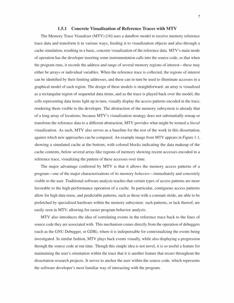
1.5.1 Concrete Visualization of Reference Traces with MTVThe Memory Trace Visualizer (MTV) [16] uses a dataflow model to receive memory reference
trace data and transform it in various ways, feeding it to visualization objects and also through a
cache simulation, resulting in a basic, concrete visualization of the reference data. MTV’s main mode
of operation has the developer inserting some instrumentation calls into the source code, so that when
the program runs, it records the address and range of several memory regions of interest—these may
either be arrays or individual variables. When the reference trace is collected, the regions of interest
can be identified by their limiting addresses, and these can in turn be used to illuminate accesses in a
graphical model of each region. The design of these models is straightforward: an array is visualized
as a rectangular region of sequential data items, and as the trace is played back over the model, the
cells representing data items light up in turn, visually display the access patterns encoded in the trace,
rendering them visible to the developer. The abstraction of the memory subsystem is already that
of a long array of locations; because MTV’s visualization strategy does not substantially remap or
transform the reference data to a different abstraction, MTV provides what might be termed a literal
visualization. As such, MTV also serves as a baseline for the rest of the work in this dissertation,
against which new approaches can be compared. An example image from MTV appears in Figure 1.1,
showing a simulated cache at the bottom, with colored blocks indicating the data makeup of the
cache contents, below several array-like regions of memory showing recent accesses encoded in a
reference trace, visualizing the pattern of these accesses over time.
The major advantage conferred by MTV is that it allows the memory access patterns of a
program—one of the major characterizaitons of its memory behavior—immediately and concretely
visible to the user. Traditional software analysis teaches that certain types of access patterns are more
favorable to the high-performance operation of a cache. In particular, contiguous access patterns
allow for high data reuse, and predictable patterns, such as those with a constant stride, are able to be
prefetched by specialized hardware within the memory subsystem: such patterns, or lack thereof, are
easily seen in MTV, allowing for easier program behavior analysis.
MTV also introduces the idea of correlating events in the reference trace back to the lines of
source code they are associated with. This mechanism comes directly from the operation of debuggers
(such as the GNU Debugger, or GDB), where it is indispensable for contextualizing the events being
investigated. In similar fashion, MTV plays back events visually, while also displaying a progression
through the source code at run time. Though this simple idea is not novel, it is so useful a feature for
maintaining the user’s orientation within the trace that it is another feature that recurs throughout the
dissertation research projects. It serves to anchor the user within the source code, which represents
the software developer’s most familiar way of interacting with the program.

8
Figu
re1.
1.M
emory
Tra
ceV
isual
izer
(MT
V)
exam
ple
,sh
ow
ing
mem
ory
acce
sses
post
ing
toa
seri
esof
arra
y-l
ike
mem
ory
regio
ns.
9
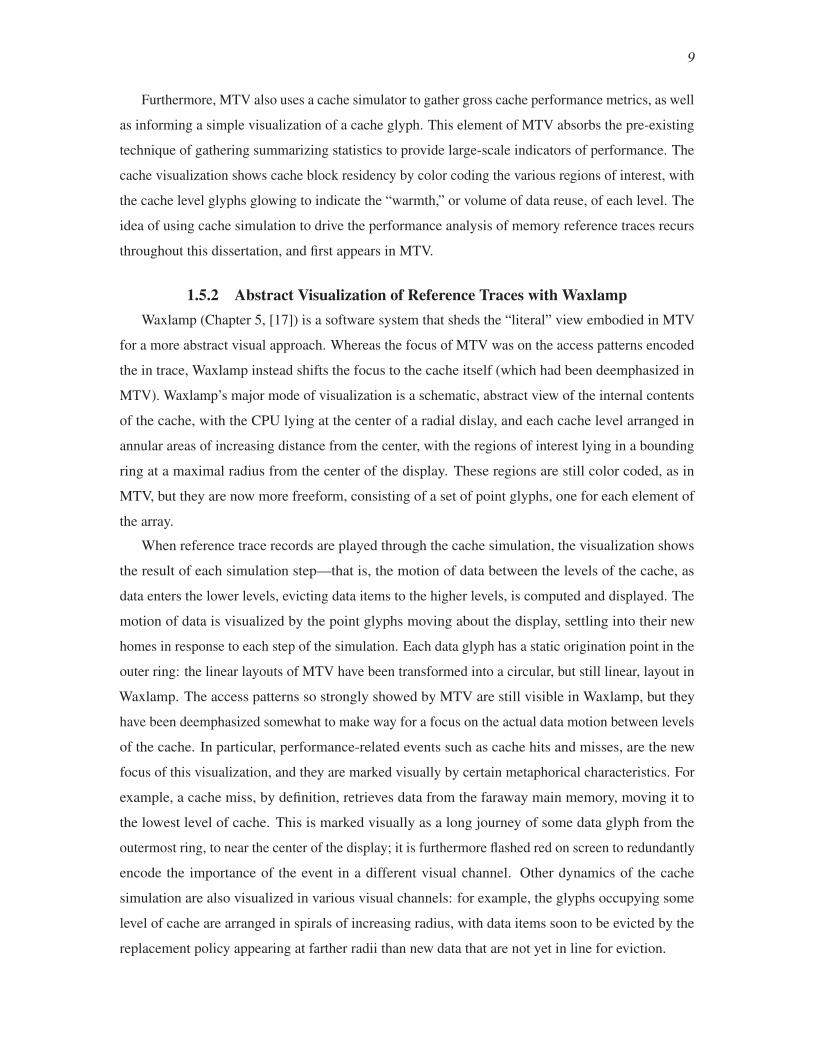
Furthermore, MTV also uses a cache simulator to gather gross cache performance metrics, as well
as informing a simple visualization of a cache glyph. This element of MTV absorbs the pre-existing
technique of gathering summarizing statistics to provide large-scale indicators of performance. The
cache visualization shows cache block residency by color coding the various regions of interest, with
the cache level glyphs glowing to indicate the “warmth,” or volume of data reuse, of each level. The
idea of using cache simulation to drive the performance analysis of memory reference traces recurs
throughout this dissertation, and first appears in MTV.
1.5.2 Abstract Visualization of Reference Traces with WaxlampWaxlamp (Chapter 5, [17]) is a software system that sheds the “literal” view embodied in MTV
for a more abstract visual approach. Whereas the focus of MTV was on the access patterns encoded
the in trace, Waxlamp instead shifts the focus to the cache itself (which had been deemphasized in
MTV). Waxlamp’s major mode of visualization is a schematic, abstract view of the internal contents
of the cache, with the CPU lying at the center of a radial dislay, and each cache level arranged in
annular areas of increasing distance from the center, with the regions of interest lying in a bounding
ring at a maximal radius from the center of the display. These regions are still color coded, as in
MTV, but they are now more freeform, consisting of a set of point glyphs, one for each element of
the array.
When reference trace records are played through the cache simulation, the visualization shows
the result of each simulation step—that is, the motion of data between the levels of the cache, as
data enters the lower levels, evicting data items to the higher levels, is computed and displayed. The
motion of data is visualized by the point glyphs moving about the display, settling into their new
homes in response to each step of the simulation. Each data glyph has a static origination point in the
outer ring: the linear layouts of MTV have been transformed into a circular, but still linear, layout in
Waxlamp. The access patterns so strongly showed by MTV are still visible in Waxlamp, but they
have been deemphasized somewhat to make way for a focus on the actual data motion between levels
of the cache. In particular, performance-related events such as cache hits and misses, are the new
focus of this visualization, and they are marked visually by certain metaphorical characteristics. For
example, a cache miss, by definition, retrieves data from the faraway main memory, moving it to
the lowest level of cache. This is marked visually as a long journey of some data glyph from the
outermost ring, to near the center of the display; it is furthermore flashed red on screen to redundantly
encode the importance of the event in a different visual channel. Other dynamics of the cache
simulation are also visualized in various visual channels: for example, the glyphs occupying some
level of cache are arranged in spirals of increasing radius, with data items soon to be evicted by the
replacement policy appearing at farther radii than new data that are not yet in line for eviction.

10
Because these visual designs are based less in the physical structure of the cache than in the
data characteristics of interest to the developer, this visualization approach is more abstract than that
offered by MTV. The abstractness leads to new patterns being visible. For instance, if a sequence
of memory activity causes a high volume of cache misses—an important performance-related
event—Waxlamp will show a flurry of data items flying in from the outer memory ring, with their
motion trails lighting up red to highlight the volume of misses. By contrast, when the hit rate is
high instead, this will be visualized as very localized activity nearer to the center of the display,
leaving the faraway contents of main memory undisturbed. More complex patterns emerge as well:
one unfortunate pattern of poor performance involves data being evicted from the cache that will
soon be needed again. This would manifest as a peculiar pattern: data items at the outer edge of a
cache level would be evicted to main memory, and then soon after re-enter the cache, resulting in
a swooping exit-and-entry arc. Such patterns have an immediate meaning that signals the need for
software analysis to the software engineer. Common program idioms, such as sweeping or striding
access patterns, or heavy usage of a small stretch of memory locations, are also concretely visible in
Waxlamp. Such an example appears in Figure 1.2, showing the initialization of a data array. The
bundle of red lines shows data coming into the cache (towards the center) from main memory (the
outer ring). As subsequent blocks are pulled in to be initialized, the bundle of red lines is seen to
sweep clockwise around the arc of the green array in memory.
The flexible, abstract design of Waxlamp’s high-level layout lends itself to other architectures
and scales as well. If performance data about some system (GPU, cluster running MPI, I/O systems,
etc.) can be collected, then it is possible to use Waxlamp’s philosophy of encoding high-latency
operations as farther distances to arrange the relevant components of the system, and play back the
performance data over it. In other words, Waxlamp generalizes the MTV approach to any system in
which data moves from place to place, and certain types or patterns of motion result in high or low
performance.
1.5.3 Computing and Visualizing the TopologicalStructure of Reference Traces
Setting aside cache simulation and the cache itself, a topological analysis approach allows focus
on the structure of the reference trace itself (Chapter 6, [19]). A reference trace is nominally a
one-dimensional, linear data source—a straightforward report of accessed addresses as a function of
time. However, program flow, and programs themselves, are inherently nonlinear, typically executing
loops, in which the flow repeats some number of times, and branches, which cause the flow to take
one path or another through the program code.
Recurrence is an important feature of program execution that can manifest in the sequence of

11
Figure 1.2. Waxlamp example. A sequence of example images from the Waxlamp system, showing
progress in initializing an array at the start of a program. The red incoming lines are showing blocks
of data being brought into the cache to be written to; the lines can be seen to sweep around the
circular arc representing the data array.
memory transactions, mapping to various types of program structures and behaviors, and also to
operations that the memory hardware can try to optimize, such as prefetching. Such recurrences can
occur at many program scales. For instance, a physical simulation may repeat a very long sequence
of actions once per timestep, constituting a large-scale recurrence. By contrast, one of these actions
may be an early data preparation step in which all the elements of some intermediate data array are
initialized to zero, constituting a much smaller-scale recurrence. Detecting and visualizing such
structures in the reference trace shows both the structure of the program itself, as well as exposing
possibly unexpected recurrences that are not as apparent in the program code.
However, finding recurrences in the reference trace is not a simple matter of looking for regions
of similarity within the trace—a recurrent behavior will repeat similar actions across some scale of
unknown size, and may contain variations within each repetition due to branching or other effects, so
that exact or even approximate matching techniques will not work. Instead, a topological approach
that treats the reference trace as a higher-dimensional point cloud, then searches for circular paths of
different sizes within it, can more effectively expose the recurrences.
The trace is converted to a point cloud by considering a sliding window of several memory
references as single points. As the window slides, the group of memory transactions represents
some sequence of actions at a particular time. In other words, the trace is converted from a single-
dimensional signal to a multidimensional one that encodes not just the actions taken at some moment,
but the contextual actions taken after that time as well. The space in which these high-dimensional
points live is then equipped with a metric function that expresses the similarity between two points,
or groupings of memory activity. Within this metric space, the points are formed by proximity into
a complex of simplices, which is then searched for circle-valued functions, which represent the

12
possible recurrent behaviors. Sorting these cycles by their persistence reveals significant program
structures.
Each of the discovered cycles with sufficiently high persistence can be visualized in a spiral,
where the angular position is given by the output from the topological method, and radius from the
center determined by time. The result is a spiral shape representing the recurrent behavior, with other
behaviors appearing within the spiral as nonspiral shapes. By shifting from one cycle to another,
various recurrent behaviors can be visualized in the same space (Figure 1.3). These images serve as
visual signatures of the recurrent behaviors in a given program, sometimes displaying unexpected or
hidden program behavior, and in some cases even suggesting possible ways to restructure computation
for higher efficiency.
1.5.4 Visualizing Differential Behavior in Reference TracesUsing Cache Simulation Ensembles
Finally, cache simulation ensembles—in which multiple reference traces are simulated in a
cache, or a single reference trace is simulated in several cache configurations—are visualized to
investigate the difference in behavior between the ensemble elements. Such ensembles are generally
formed to scientifically test the variation of some variable. For example, simulating a reference
Figure 1.3. Topological approach example. Two examples of topological visualization of a portion of
a reference trace, showing the interpolation of physical quantities from particles to a two-dimensional
grid. The left image shows the repetitive nature of computing interpolation kernels in the x and ydimensions, while the right image emphasizes the noninterpolation activities in the expanding circles
(showing the interpolation activity in the zigs and zags visible in the upper portions of each circle).
13
trace through several caches differing only in size enables a study of effect that cache size has on
some algorithm. By contrast, reference traces from several implementations of the same algorithm
can be simulated through a single cache to form an ensemble that enables the study of the relative
memory performance of these implementation choices. In other words, this technique enables the
study of differential performance due to some changing quality or quantity, using a straightforward
comparative visualization of the ensemble to reveal performance differences.
Generally speaking, a programmer has no control over the choice of cache that is used at run
time. However, it is still useful to form and investigate the behavior of cache ensembles, as forming a
differential may actually reveal unexpected features of the program execution, which is under the
programmer’s control. For example, changing the cache’s block replacement algorithm in the cache
ensemble may reveal that a particular replacement algorithm leads to optimal cache behavior for
some algorithm. The cache ensemble analysis may suggest that some feature of the computation
causes it to perform well under a different policy; the programmer may then realize that it is possible
to restructure the computation in a nonobvious way so that it now aligns with the replacement that
exists in the real cache. Such an example, along with many others, appears in Chapter 6. An example
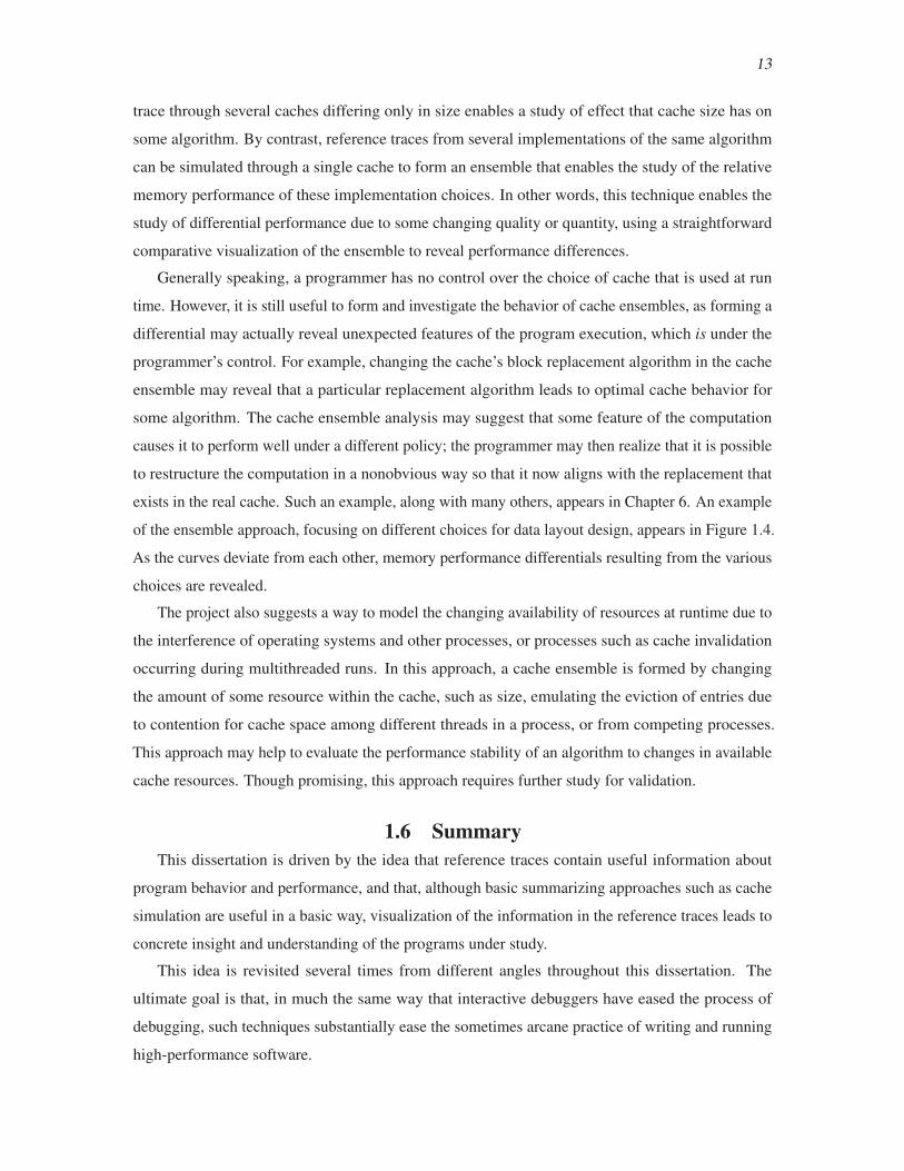
of the ensemble approach, focusing on different choices for data layout design, appears in Figure 1.4.
As the curves deviate from each other, memory performance differentials resulting from the various
choices are revealed.
The project also suggests a way to model the changing availability of resources at runtime due to
the interference of operating systems and other processes, or processes such as cache invalidation
occurring during multithreaded runs. In this approach, a cache ensemble is formed by changing
the amount of some resource within the cache, such as size, emulating the eviction of entries due
to contention for cache space among different threads in a process, or from competing processes.
This approach may help to evaluate the performance stability of an algorithm to changes in available
cache resources. Though promising, this approach requires further study for validation.
1.6 SummaryThis dissertation is driven by the idea that reference traces contain useful information about
program behavior and performance, and that, although basic summarizing approaches such as cache
simulation are useful in a basic way, visualization of the information in the reference traces leads to
concrete insight and understanding of the programs under study.
This idea is revisited several times from different angles throughout this dissertation. The
ultimate goal is that, in much the same way that interactive debuggers have eased the process of
debugging, such techniques substantially ease the sometimes arcane practice of writing and running
high-performance software.
14
��
��
��
�
���������������� ������
����� �������� ��������
Figu
re1.
4.E
nse
mb
leap
pro
ach
exam
ple
.A
nex
amp
leo
fv
isu
aliz
ing
aca
che
sim
ula
tio
nen
sem
ble
,in
wh
ich
ap
arti
cle
syst
emh
asit
sd
ata
sto
rag
ela
id
out
info
ur
dif
fere
nt
way
s.W
her
eth
ecu
rves
dev
iate
from
each
oth
er,a
mem
ory
per
form
ance
dif
fere
nti
alis
hig
hli
ghte
d,pro
vid
ing
evid
ence
for
or
agai
nst
apar
ticu
lar
choic
eof
layout.
The
lett
ered
segm
ents
refe
rto
vari
ous
par
tsof
the
algori
thm
,in
whic
hdif
fere
nt
types
of
acti
vit
yre
sult
indif
fere
nt
mem
ory
beh
avio
rsi
gnat
ure
s.
CHAPTER 2
TECHNICAL BACKGROUND
This chapter discusses some existing technologies, techniques, and approaches that are made
use of in this dissertation. In particular, the nature of caching is described, and how software
instrumentation and simulation are used to produce memory reference traces, the fundamental source
of data used for the research projects in this dissertation.
2.1 Caching in Computer SystemsFundamentally, a cache is a fixed amount of storage for holding a limited number of copies of
data items that are more permanently stored in some other place. The purpose of having a cache
is to enable fast access to the cached data, as opposed to retrieving the same data items from their
permanent storage locations.
Computer systems use many kinds of caches. Any time that data must be retrieved from its native
source slowly, caches can be useful. For example, web browsers can keep cached copies of webpages
whenever they are first loaded. Retrieving a local, cached copy of a webpage is much faster than
retrieving the same page via network protocols from a remote machine—as the cached copy is loaded
for the user to look at, the browser can begin to load a fresh copy from the network to make sure the
user is looking at the newest version of the document. In this case, the local disk acts as a cache for
the remote machine, where the “true” webpages reside.
The memory system can likewise serve as a cache for data residing on disk, since disk access
latency is several orders of magnitude slower than memory access latency. For example, when
launching a program, operating systems tend to load the program code and data into memory before
beginning execution, rather than reading the program code directly from disk at runtime. However,
there are also more application-specific uses of memory as a cache for the disk in cases when,
for example, large amounts of data are being processed in random-access orders. For example, in
large-scale visualization [13, 67] it may be necessary to predict which parts of the data will be needed
in the near future, and therefore ensure that they are read from disk into memory, so that the algorithm
can access them from memory rather than having to load them—much more slowly—from disk.
16
The memory system itself makes heavy use of caching to accelerate access to data residing there.
These caches are usually implemented in hardware, as they have dedicated jobs with predefined
rules of operation. For example, operating system level memory management uses a translation
lookaside buffer (TLB) to accelerate the retrieval of memory pages for programs performing memory
access. The operating maintains a page table—stored in a dedicated area of memory—to map from a
program’s virtual addresses to the physical memory addresses of the corresponding pages of memory.
Without the TLB, for each memory access request, the operating system would have to consult the
page table, and then look up the resulting physical page, roughly doubling the time spent in memory
lookups. The TLB instead stores a small number of page table entries in a hardware cache, which can
be looked up much faster than the page table itself. Because the TLB, like all caches, has a limited
size, at some points during execution, the operating system will still need to consult the page table,
but the presence of the TLB limits how often this must be done.
The example of the TLB hits upon one of the fundamental qualities of hardware caches: they
are fast by necessity and design; however, their speed dictates that they also be either small, or
expensive. For this reason, the major tradeoff in caching systems is between speed and size. This
pattern recurs in other examples of hardware caches. For instance, NVIDIA graphics processing units
(GPUs) contain two kinds of memory: “global memory” that is slow to access (taking on the order
of hundreds of cycles) but very large, and a much smaller “shared memory” that can be accessed
within just a few cycles. In older GPUs, the programmer has the option of using the shared memory
as a cache, carefully managing what data is loaded into it from the slower global memory, striving to
allow the processors to use this data as much as possible before loading in a new set of data from
global memory. In fact, if the programmer does not use the shared memory as a cache, it is difficult
or impossible to achieve the high-performance promise of the GPU. More recent models offer the
alternative of automatic caching of global memory accesses, again in the shared memory, much like
that found in CPU memory caches—the particular focus of this dissertation.
2.1.1 CPU Memory CachesIn the manner of the caching examples discussed above, the CPU memory cache is used to store
a small subset of data residing natively in memory to enable fast access to it, and as with the TLB, its
major design tradeoff is in speed versus size. The idea behind this cache is that, as a program makes
memory references, the CPU retrieves the requested data from the memory system (at great cost)
and caches a copy in the cache. If the program happens to make another reference to the cached
data, it can be retrieved—at relatively very little cost—from the cache instead of memory. The
composition and arrangement of the cache is important to understanding how it works. For instance,
when the cache is full, and an access to a nonresident piece of data is made, some decision needs to

17
be made about which resident piece of data to evict to make way for the new data. Because such
design parameters have a definite and significant effect on performance, this section describes the
components of a cache, how they work together, and the rules under which they operate to provide
caching services for main memory.
2.1.1.1 Cache Design and OperationThe memory subsystem consists of main memory—a generally large array of locations in which
data can be stored and manipulated when a program runs—and a CPU memory cache (Figure 2.1).
The cache stores some subset of the contents of memory, enabling faster access to this subset. A
cache consists of several cache levels arranged with a certain relationship, described below. When a
program requests some data from the memory subsystem, it is first sought in the cache, level by level.
If the data is found, it can be copied into the registers for use by the program immediately; if not, a
sequence of protocols governs how the data is copied from main memory into the levels of the cache
(possibly evicting some data that had been present in the cache already), and from there it can be
copied into the registers as well.
Each cache level contains some amount of storage, divided into an array of fixed-size divisions
known as cache blocks or cache lines. The size of a cache block is constant for all levels of a
given cache. The cache block is the fundamental, atomic unit of data packaging for the memory
system—that is, when a program makes an access to some address, it is the entire cache block
containing that address that is copied from main memory into the cache. This is to take advantage of
spatial locality, the notion that in typical programs, when an address is accessed, nearby addressed
tend to be accessed soon after. In other words, by transferring a whole block, the cache tends to have
related data ready for access.
Just as each location in memory has an address, so too do the cache blocks. The block address
of the cache block containing a given location is simply some prefix of the address of the item at
that location. As an example, 0x1000ccee is a 32-bit address for some location in memory. For
256-byte cache blocks, the containing block’s address would be 0x1000cc, and the items contained
within it would have addresses ranging from 0x1000cc00 to 0x1000ccff (with 256 addresses
represented in the lower 8 bits).
2.1.1.1.1 Set associativity. To place a block of data into a level, the cache must decide which
block it will occupy. The simplest placement policy is called direct-mapping, in which each block has
a single place in the level it can go. Generally, the mapping is derived from the cache block address.
Once more taking the example of cache block address 0x1000cc, and assuming a direct-mapped
cache level of 128 cache blocks, the block would be placed in the 0x1000cc mod 128 = 76th block
of the cache level.

18
������������ �
(a)
����� ����� ����� ����
(b)
�����
������������
�������
�����
(c)
Figure 2.1. The memory subsystem. (a) A schematic view of the memory subsystem. The cache
levels are L1, L2, and L3; each is larger and slower than the last, so the programmer strives to be
able to retrieve necessary data from the fastest possible level. Beyond L3 lies main memory, which is
much larger and slower than any of the cache levels. (b) A zoomed view of a particular cache level.
The level has four associative sets into which incoming blocks may be placed. The mapping from a
block to a set is a function of the block’s address in memory; once assigned to a set, it may be placed
anywhere within it. (c) A zoomed view of a particular set, made up of eight blocks (making this
cache level 8-way set associative). Supposing that the size of the cache block is 16 bytes, block 0
is seen to contain four 4-byte data items (perhaps single-precision floating point numbers), block 1
contains two 8-byte items (perhaps double-precision floating point numbers), while block 7 contains
a single 16-byte item (perhaps a struct containing other data). These items, represented by different
colored shapes, are the items addressed by name in a program; this diagram shows how such data
items are arranged into cache blocks residing in cache sets, which are arranged into cache levels,
which ultimately form a cache serving requests for data from main memory.
19
Though direct-mapping has a straightforward block placement algorithm, and it requires simpler
circuitry to implement, it often results in different memory blocks contending for the same space
within the cache. To remedy this problem, caches can have a set associative design, in which the
cache blocks in a given level are grouped into sets. Incoming data, rather than being specifically
assigned to a single cache block, is now associated with a particular set; the data can go anywhere
within this set, reducing contention. At one extreme, all of the blocks can be grouped into a single
set, resulting in a fully associative cache level. More generally, for sets of N blocks, the cache is said
to be N-way set associative. Under this terminology, “direct-mapped” is simply a special name for
“1-way set associative,” while “fully associative” denotes “S-way set associative,” where the level has
S blocks.
2.1.1.1.2 Block replacement policy. Even set associative caches, however, need a way to
select a block to replace when a new block enters. This forced removal is called eviction, and the
removed block is called the victim. Given a full cache level and an incoming block, the level’s block
replacement algorithm or block replacement policy selects which block to evict. Since incoming
blocks are restricted to a particular set, this amounts to selecting a victim from the target set. No
such algorithm is needed for direct-mapped caches, which have only a single block per set, which is
by necessity always the victim block.
The goal of a replacement policy is to minimize the number of future evictions, as these occur only
when requested data is not found in the cache. It has been proven that the optimal algorithm is the one
that chooses the evict the block that will not be needed for the longest time in the future [6]. Because
the future memory behavior of a given program is not generally known at run time, this algorithm,
known as “OPT,” cannot generally be implemented for use. The goal of real replacement policies
is therefore to approximate OPT as well as possible. There is also a policy named “PES”—dual
to OPT—that selects the block that will be needed the soonest. This “pessimal” policy attempts to
cause as many evictions as possible. Though this policy is clearly not useful for real systems, it,
along with OPT, can be useful in cache behavior analysis (see Chapter 7).
A commonly used replacemnt policy evicts the least-recently used (LRU) block in the set, under
the motivation that past behavior can model future behavior. Essentially, the block that has not been
used for the longest period of time is implicitly assigned the lowest probability among all blocks in
the set of being the first to be accessed in the future, and is therefore evicted. There are perverse cases
in which LRU gives exactly the wrong prediction (see Chapter 7); for such cases, most-recently used
(MRU) may be a better replacement policy. To implement LRU and MRU, the cache level would
require circuitry to register the last-access time of each block in the set, imposing a cost in economic
and performance terms on such hardware. However, the efficacy of a policy such as LRU makes such
20
costs generally bearable.
Another simple policy, named “RANDOM,” is to simply select a victim block at random. This
policy has the advantage of a simpler implementation, but has no principle behind it to try to drive
down the eviction rate. In this dissertation, RANDOM can be used as an indicator of a middle ground
for eviction rates, contrasting with the optimal behavior of OPT and the pessimal behavior of PES,
forming a spectrum of possible cache behaviors.
2.1.1.1.3 Cache composition and operation. A cache level is then defined by how many
blocks it contains, how many sets the blocks are divided into, and how the level selects a victim block
when there is no room for a new incoming block of data. A cache level is then capable of being used
as a cache for data coming from some other source, either main memory, or another, larger cache
level. A cache, in general, is built from a sequence of increasingly larger cache levels, with each
level caching data from the next. The levels are generally labeled “L1,” “L2,” and so on.
To read data from memory, the processor issues a request for the target address to the cache. The
cache hardware searches for the corresponding block in the levels (first by locating the set that block
would reside in, then search the blocks of that set). Supposing the block is present in level L of the
cache, the data in the block is first copied to levels 1 through L−1, and the processor is then able to
copy the appropriate values to a processor register. If the processor needs any data from that block in
the near future, it will be found in L1, with the fastest transfer time. This situation is known as a read
hit, because the data was found in cache and there was no need to go to main memory to retrieve the
data. On the other hand, when the data is not found in cache, this is called a read miss, and it incurs a
performance penalty due to the much longer latency of retrieving data from main memory.
Writing to memory is a little bit different: if an entry in the cache is modified, but the backing
entry in main memory is not, in some sense the memory system is inconsistent. To this end, a cache
level can be designated as write-through, meaning that when writes are posted to a block in that level,
the write continues “through” the level to the next higher one (where, in recursive fashion, the same
thing may happen if that level is also write-through). Alternatively, the level may be write-back,
meaning that writes “stop” at that level; however, the level keeps track that a change has been made
with a dirty flag. If a dirty block is evicted from the level, at that time the write will propagate to
the next level, so that the modifications to the block are not lost. The benefit in performance is that
several writes to the same block will only result in at most a single access to a higher cache level. As
with the read operations, when data is found in the cache, it is called a write hit; otherwise, it is a
write miss.
The cache, with its several levels, and main memory, together with the logical rules of operation,
form the memory subsystem. Conceptually, therefore, main memory can be thought of as an
21
extremely large, extremely slow level of cache. One may then speak of where in the memory
subsystem a given read hits: what is generally known as a cache miss can be retermed a “hit to main
memory.” Similarly, an access that hits to main memory can be said to have missed in L1, L2, etc.
This distinction is important in the implementation details of a cache simulator, and in analyses in
which the level of cache where data was found is important (for example, Chapter 7).
As an example of a real-world cache, consider the cache for the Intel Core i7 [8]. This cache
has three levels with a block size of 64 bytes: L1 is 32KB and 8-way set associative, L2 is 256KB
and also 8-way set associative, and L3 is 8192KB and 16-way set associative; each level uses LRU
for the block replacement policy. According to HP Labs’ CACTI tool for estimating the physical
properties of hardware caches [87], the access times for L1, L2, and L3 are 0.98 ns, 1.08 ns, and 2.85
ns respectively. By contrast, DRAM access time is on the order of 30 ns, while disk access times (in
case virtual memory on disk must be used as a backing store for DRAM) are on the order of 5 ms.
Then, the factor of slowdown between each pair of adjacent levels is: 1.1x for L1 to L2, 2.6 for L2 to
L3, 10x from L3 to DRAM, and 200000x for DRAM to disk. These numbers give some sense of
why it can be important to manage data within the cache so it found in the faster levels as often as
possible.
2.1.1.2 Cache SimulationCache simulation is an important and inexpensive way to investigate the behavior of a wide
range of cache designs [92], yielding insight into the memory performance of simulated or measured
programs. Dinero [28] and CacheGrind [61] are examples of research cache simulators providing
different types of information. Cache simulators generally work by taking as input a memory
reference trace—a list of all memory accesses performed by a program at runtime. Each record in
the trace represents a single memory transaction; these are fed one by one into the simulator, which
then computes the effect each would have on the state of the cache (using some notion of the logic
and operation of caches, such as that discussed above). The simulator then outputs statistics or other
information about cache performance, behavior, or both.
For the work in this dissertation, a custom cache simulator, named debit, has been developed
that can be extended to provide the exact level of insight into the simulation as needed. For example,
in the MTV project (Chapter 4), the visualization only needs to know what level of cache the latest
access hits to, whereas the cache ensemble analysis project (Chapter 7) requires the full history of “hit
levels” to carry out its analysis. Similarly, Waxlamp (Chapter 5) requires more structured information
about what happens during each step of simulation—for example, which level the hit occurred in,
which (if any) blocks were evicted, and other details about how data moves about between the levels
of cache. In all three cases debit, using a constant core simulation approach, was extended to
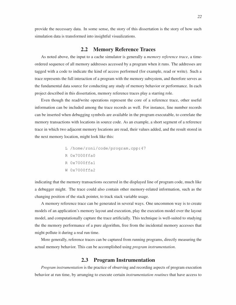
22
provide the necessary data. In some sense, the story of this dissertation is the story of how such
simulation data is transformed into insightful visualizations.
2.2 Memory Reference TracesAs noted above, the input to a cache simulator is generally a memory reference trace, a time-
ordered sequence of all memory addresses accessed by a program when it runs. The addresses are
tagged with a code to indicate the kind of access performed (for example, read or write). Such a
trace represents the full interaction of a program with the memory subsystem, and therefore serves as
the fundamental data source for conducting any study of memory behavior or performance. In each
project described in this dissertation, memory reference traces play a starring role.
Even though the read/write operations represent the core of a reference trace, other useful
information can be included among the trace records as well. For instance, line number records
can be inserted when debugging symbols are available in the program executable, to correlate the
memory transactions with locations in source code. As an example, a short segment of a reference
trace in which two adjacent memory locations are read, their values added, and the result stored in
the next memory location, might look like this:
L /home/roni/code/program.cpp:47
R 0x7000ffa0
R 0x7000ffa1
W 0x7000ffa2
indicating that the memory transactions occurred in the displayed line of program code, much like
a debugger might. The trace could also contain other memory-related information, such as the
changing position of the stack pointer, to track stack variable usage.
A memory reference trace can be generated in several ways. One uncommon way is to create
models of an application’s memory layout and execution, play the execution model over the layout
model, and computationally capture the trace artificially. This technique is well-suited to studying
the the memory performance of a pure algorithm, free from the incidental memory accesses that
might pollute it during a real run time.
More generally, reference traces can be captured from running programs, directly measuring the
actual memory behavior. This can be accomplished using program instrumentation.
2.3 Program InstrumentationProgram instrumentation is the practice of observing and recording aspects of program execution
behavior at run time, by arranging to execute certain instrumentation routines that have access to
23
program state at various times during execution. One way to instrument a program is statically, by
inserting extra source code to record data about its own execution; this can be accomplished using,
for example, a source-to-source compiler such as ROSE [73]. This approach is somewhat limited,
however, as it can only affect portions of the program for which source code is available, causing
possibly cumbersome changes the code itself, and requiring a rebuild before the instrumentation
can become active. Furthermore, the instrumentation code may affect how the compiler handles the
program, possibly causing so-called “Heisenberg effects,” in which observing the program directly
changes what is observed.
Alternatively, dynamic instrumentation, which can overcome these limitations, works by running
the target program, but observing its execution, and trapping to predefined instrumentation routines
when specific trigger actions occur in the program. Pin [52] is a library and API for building dynamic
instrumentation routines that works by dynamic binary rewriting. Pin works by controlling the
execution of the target program; as it runs, and the trigger actions occur, Pin actively rewrites the
incoming instruction stream in memory, modifying it to make calls to the user’s instrumentation
routines.
To create a Pin program for capturing a memory reference trace, the program is instructed to
trap to recording routines whenever a memory instruction (i.e., a read or write operation) is to
be executed. The recording routines have access to the target address of the memory instruction,
and can therefore record the read/write code, and the target address, to produce trace records such
as the ones in the example above. To produce the source code record lines, the Pin program can
examine each instruction before it executes, looking up the instruction address in the program’s
symbol table, and recording the appropriate information in the reference trace. The Pin API provides
routines with many kinds of insight into the program state, enabling the recording of many kinds of
information. In environments where Pin (or some other library like it) can run, it provides an ideal
method of collecting a memory reference trace. In other environments (such as a program executing
on special-purpose hardware, like a graphics card) it may not be possible to engage in dynamic
instrumentation methods, so some simpler method such as static instrumentation must be used.
CHAPTER 3
RELATED WORK
This dissertation is about investigating the behavior of the memory system during program
run time, towards the end of understanding and possibly improving the performance thereof. The
major approach is using reference traces to drive cache simulations, then visualizing the results. To
contextualize those ends, this chapter presents a broad overview of related work in all three involved
fields: performance analysis and visualization, software visualization, and reference trace processing.
3.1 Performance Modeling, Analysis, and VisualizationAs discussed in Chapter 1, software performance is sometimes a concrete software design goal,
when very large problems must be solved, or when computational resources are scarce and must
be used efficiently. Generally speaking, software performance refers to the optimization of some
measure during program run time—commonly speed, or the total time it takes to compute a result, but
also other quantities associated with limited resources, such as power consumption. This dissertation
is focused on program speed, although with an appropriate data source, some of the techniques
presented herein could be adapted for other metrics as well.
3.1.1 ToolsThe classical way to measure program speed is by using a software profiler, which observes a
running program and collects statistics about how much time it spends in various functions and lines
of source code. GNU GProf [33], Intel VTune [43], and Apple Shark [2] are examples of software
profilers. Profilers collect performance data and generally display it textually, with links to source
code and the call stack, enabling debugger-like exploration of the program’s performance behavior.
The basic usage pattern is to run a program, allow the profiler to collect and display performance
data, and then home in on areas of the program source code that contribute the most heavily to overall
run time. Such areas are possible candidates for optimization, though the profiler cannot generally
describe why these regions of code associate with longer relative run times.
25
Many profilers can access the machine’s hardware performance counters, which are special-
purpose read-only registers that count certain performance-related events, such as cache misses,
and create simple graphs of the resulting data. This data provided is coarse-grained, and useful for
spotting trends in behavior over longer time scales. Generalizing this capability, software libraries
such as PAPI [89] provide an API to these performance counters, granting any application some
insight into its own performance characteristics.
3.1.2 High-Performance Software TechniquesSoftware developers have a portfolio of techniques that tend to improve software performance.
Among the most basic is to use algorithms with low asymptotic time complexity [20]—for example,
selecting quicksort or merge sort, with their O(n logn) complexity, over bubble sort, which is O(n2).
The work in this dissertation is focused on examining how a particular implementation behaves with
respect to the memory system. In this context—after algorithm selection—there are more software
techniques for attempting to achieve high performance by engaging the available hardware in specific
ways.
Identifying and running logically independent streams of computation concurrently, or paralleliz-
ing software, can improve performance a great deal by overlapping the execution of required tasks
on a multiprocessor machine. Within each thread of computation, programmers can try to improve
memory caching behavior by using tiling or bricking of application data in specific ways [67] to try
to match the cache presence of data with the order of operations in the code. More generally, cache
oblivious algorithms [71] and data layouts [98] are designed to show relatively good cache behavior,
regardless of a particular cache’s design parameters.
Out-of-core methods are used to achieve acceptable performance on very large data that cannot
fit into memory (“core”) all at once. Out-of-core techniques can be used for processing of very large
meshes obtained from 3D scanners [44], clustering in mining very large data sets [55], managing data
for visualization [13] and scenes for graphics applications [14] predictively, performing numerical
computation on very large input matrices [90], among many other applications.
In contrast to the use of such software approaches, along with programs such as profilers, to
build and measure high-performance software, performance prediction is used to model the predicted
performance of a new or as-yet undesigned supercomputer on current software, using data from
existing computers [48]. Much as simulation is used by scientists to reduce or avoid the cost of
physical experimentation, such performance modeling can help architects design new machines for
use on known problems, tailoring them to meet their expected demands.

26
3.1.3 Visualization ApproachesThough profilers provide valuable data about program performance, they generally provide
textual display, or, at best, simple graphs of some of this data. Vampir [58] and TAU [79] perform a
deeper data collection and visual analysis of performance data from parallel programs. They collect
execution traces from instrumented parallel programs at runtime, then provide various kinds of
statistically guided displays of the data, layered onto visual models of interactions between compute
nodes, run time in various parts of the programs, etc. This approach provides deeper insight than
the simpler behavior and displays of code profilers, enabling the developer to investigate causes of
slowdown by seeing how the parallel threads interact, and the resulting performance numbers.
Vampir and TAU provide very general visualization facilities, in contrast to more subsystem-
oriented visualization approaches that can take specific knowledge and understanding of smaller-scale
components of the computer system. These are described below, in the broader context of software
visualization.
3.2 Software VisualizationSoftware visualization is a relatively young subfield of visualization, in which data about software,
in all its incarnations, is visualized, with the end goal of providing insight about all aspects of
software—construction, evolution, structure, execution, behavior, performance. At its core, this
dissertation is about software visualization, focused upon the memory subsystem. As such, this
section gives a detailed overview of the various genres of software visualization, while providing
references on classic and current work in the field. A structured treatment of software visualization
on the whole can be found in Diehl’s textbook [25].
Work in software visualization can be divided into two broad camps: static approaches, which deal
with software in all its forms before it executes; and dynamic approaches, which deal with software
when it runs. The work in this dissertation falls primarily under dynamic software visualization, but
ideas from static program visualization are also present as contextualizing and framing devices.
3.2.1 Static Software VisualizationStatic software visualization is concerned with visual representations of software before it
executes—that is, it is all about the structure of software, its relationship to other pieces of software,
and the way software changes during the development cycle.
Static analysis [62] computes qualities of a piece of software without actually running it: put
another way, it deals in statements about the software that must hold true for its every possible
execution. Perhaps the most famous result from static analysis is Turing’s proof of the undecidability

27
of the halting problem [91], which is a statement about all possible programs running on a particular
kind of computational model.
3.2.1.1 Control Structure VisualizationLess broadly, many kinds of information about a program can be computed from its source
code. For instance, one very simple approach—that may or may not be considered to be actual
visualization—is syntax highlighting and automatic indentation in text editors and integrated
development environments. Source code generally contains a tree-like syntax structure, according
to the rules of some programming language, and highlighting keywords and indenting the nested
subtree structures constitutes a visual representation of that structure, one that many programmers
find indispensable in writing programs.
Other classic visual approaches to representing the structure of programs are diagrammatic
in nature. Jackson diagrams [45], control-flow graphs [36], “structurograms” [59], and control-
structure diagrams [21] are different ways of plotting the structure and flow of program code
elements, including sequences of statements, conditional execution (i.e., if-statements), and loop
repetition (i.e., for-statements). These approaches are meant to transform the linear sequence of text
constituting a program into spatial representations of the different ways in which program flow might
run during execution. Programs such as StackAnalyzer [30] can provide both static and dynamic
control-flow graphs for live programs.
3.2.1.2 Visualizing Software ArchitectureAt a longer perspective, the details of code syntax fade into the software architecture—the
structure of the larger-scale software components and how they relate to each other. Architecture is a
primary concern of software design, and good architectural designs lead to well-understood, easily
maintainable software [5]. To this end, it can be useful to visualize the architecture of a software
project.
3.2.1.2.1 Diagramming. Drawing informal diagrams on paper or whiteboards is an indispens-
able planning technique for software developers. Koning et al. [51] analyze common practices and
suggests standard guidelines for such architecture drawings, while Walny et al. [94] follow several
developers with very different work habits, analyzing their use of drawings and their evolution. By
contrast, the Unified Modeling Language (UML) [31] is a standardized set of graphical symbols
used to visually model many aspects and phases of software design and creation, including sequence
diagrams for modeling the order of events, class diagrams for modeling functional and logical
relationships between programming objects, and use-case diagrams for modeling possible contexts
for users engaging software, among many others.

28
3.2.1.2.2 Visualization. Direct architecture visualization of larger software projects can be
helpful for navigating large amounts of code quickly. For example, automatic layout generation
algorithms show the structural relationships between classes, as well as their function call relation-
ships [29]. Visual metaphors can also be used to transform software architecture into other familiar
settings. For instance, the Software Landscapes approach [3] creates islands for each class, with
buildings on the islands representing methods. Generalizing the idea of islands in a sea, the Software
World approach [49] treats the project itself as a planet, with packages, files, classes, and methods
being represented by countries, cities, districts, and buildings, respectively, with features of the
buildings (height, doors, windows, etc.) representing particular features of methods (such as method
length, parameter types, variables, etc.). An extension to this approach [64] suggests including some
dynamic information in these software worlds, using fires in buildings to represent often-executed
methods, and showing dataflow from entity to entity using cars and boats traveling along one-way or
two-way roads and waterways.
Visualization approaches can also be used to depict the evolution of software systems, tracking
developer behavior and software changes, as reported by, e.g., a software versioning system’s history
data. For example, if a cityscape can represent the structure of a software system, then software
evolution can be visualized as a growing city [83], extending the metaphor to include history. The
Code Swarm project [63] uses a more organic approach [32] to provide a developer-centric view of
software evolution, in which developers are representing by small lit points that swarm around the
files they are working on, showing activity on the whole, and also concentrated around “hot” items
that receive frequent updates.
3.2.2 Dynamic Software VisualizationWhen software actually runs, it engages in a complex exchange of code and data with the
hardware it runs on, producing interactions that can be the subject of visualization, to reflect the
behavior of the program, as opposed to just its structure. The work in this dissertation, being
concerned with capturing and visualizing the runtime memory behavior of programs, falls into this
broad division of the field. This section reviews some of the major themes in the subfield, while
pointing out connections and contexts for the dissertation work where they exist.
3.2.2.1 Visual Programming and DebuggingVisual programming is the activity of arranging software modules or programming elements
graphically, connecting them together to form programs. Scratch [53] is an educational programming
language in which standard programming elements (assignment, operators, for- and while-loops,
if-statements, etc.) take visual form, possibly allowing for embedding of other statements within
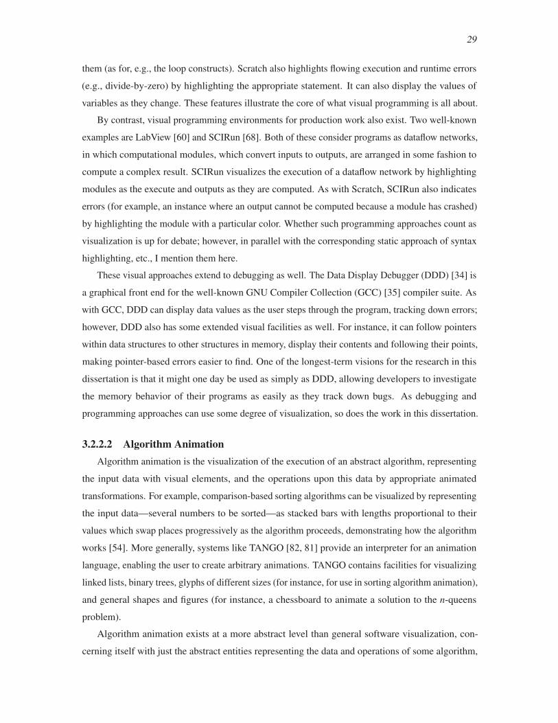
29
them (as for, e.g., the loop constructs). Scratch also highlights flowing execution and runtime errors
(e.g., divide-by-zero) by highlighting the appropriate statement. It can also display the values of
variables as they change. These features illustrate the core of what visual programming is all about.
By contrast, visual programming environments for production work also exist. Two well-known
examples are LabView [60] and SCIRun [68]. Both of these consider programs as dataflow networks,
in which computational modules, which convert inputs to outputs, are arranged in some fashion to
compute a complex result. SCIRun visualizes the execution of a dataflow network by highlighting
modules as the execute and outputs as they are computed. As with Scratch, SCIRun also indicates
errors (for example, an instance where an output cannot be computed because a module has crashed)
by highlighting the module with a particular color. Whether such programming approaches count as
visualization is up for debate; however, in parallel with the corresponding static approach of syntax
highlighting, etc., I mention them here.
These visual approaches extend to debugging as well. The Data Display Debugger (DDD) [34] is
a graphical front end for the well-known GNU Compiler Collection (GCC) [35] compiler suite. As
with GCC, DDD can display data values as the user steps through the program, tracking down errors;
however, DDD also has some extended visual facilities as well. For instance, it can follow pointers
within data structures to other structures in memory, display their contents and following their points,
making pointer-based errors easier to find. One of the longest-term visions for the research in this
dissertation is that it might one day be used as simply as DDD, allowing developers to investigate
the memory behavior of their programs as easily as they track down bugs. As debugging and
programming approaches can use some degree of visualization, so does the work in this dissertation.
3.2.2.2 Algorithm AnimationAlgorithm animation is the visualization of the execution of an abstract algorithm, representing
the input data with visual elements, and the operations upon this data by appropriate animated
transformations. For example, comparison-based sorting algorithms can be visualized by representing
the input data—several numbers to be sorted—as stacked bars with lengths proportional to their
values which swap places progressively as the algorithm proceeds, demonstrating how the algorithm
works [54]. More generally, systems like TANGO [82, 81] provide an interpreter for an animation
language, enabling the user to create arbitrary animations. TANGO contains facilities for visualizing
linked lists, binary trees, glyphs of different sizes (for instance, for use in sorting algorithm animation),
and general shapes and figures (for instance, a chessboard to animate a solution to the n-queens
problem).
Algorithm animation exists at a more abstract level than general software visualization, con-
cerning itself with just the abstract entities representing the data and operations of some algorithm,
30
without regard for the particular physical implementations of those components. In this dissertation,
some of the results of the Waxlamp system (Chapter 5) dealing with sorting algorithms have some
features closely reminiscent of work in algorithm animation. Indeed, Waxlamp is providing a view of
how a particular algorithm looks with respect to memory. Although the memory subsystem is a part
of the physical implementation of a computer system, observing an algorithm’s behavior in a “real”
memory system can deliver insights about the behavior of that algorithm, and also its implementation
as “real” software.
3.2.2.3 Animation for Static DiagramsOne basic technique for visualizing runtime data about program execution is to layer such data
over a visual structure representing some static aspect of the software. SoftArch [38] is a design
tool in which the user can design a software architecture and automatically generate Java classes
whose methods are instrumented to produce runtime statistics. When the resulting program runs, the
runtime statistics can be used to colormap the elements of the static architecture diagram. Vampir [58]
and TAU [79] can similarly display static diagrams (of, e.g., call graphs, network topologies, etc.),
layering runtime information about function calls, MPI communications, etc., over them.
More generally, Stolte et al. [84] present a system in which a static, visual representation of the
internals of a superscalar processor serves as a background, over which behavior data about the
simulated processor is animated, showing how the various functional units work together to execute a
program. Whereas the work in this dissertation relies upon memory reference traces, Stolte’s system
uses a more general execution trace. This dissertation takes a similar general approach, focusing
down on the behavior of memory in particular.
This theme of extending static diagrams with animated dynamic data recurs throughout this
dissertation as well. For instance, the MTV system (Chapter 4) displays a static representation of the
simulated cache, which the changing residency of the cache blocks is represented by animated color
changes as the reference trace is played back. Similarly, Waxlamp (Chapter 5) uses a static, abstract
layout representing the internal structure of the cache, while the results of cache simulation play out
over it. The use of static diagrams and layouts as a background, while dynamic data plays back over
it, is a powerful, general technique used to great effect in the literature and this dissertation.
3.3 Reference Trace ProcessingAs discussed in Chapter 2, a memory reference trace represents a program’s full interaction with
the memory subsystem. Therefore, processing of the reference trace directly can yield insight about
memory behavior, or make it easier to work with.
31
Trace reduction refers to any technique used to reduce the size of a reference trace without
changing its essential properties. Which properties these are depends on the particular application.
For example, it is possible to transform a reference trace into a smaller trace that has the same final
effect on a simulated cache. Kaplan et al. [46] discuss two such schemes. Safely Allowed Drop
makes the observation that if some cache block B is referenced three times during some segment of
the trace, and the number of unique cache blocks other than B between the first and third reference is
smaller than the number of cache blocks in some level of the cache, then the middle reference to B
can be safely dropped from the trace, assuming a least-recently used block replacment algorithm.
In other words, assuming an LRU cache, the middle reference carries no information, and can be
discarded, thus reducing the size of the trace with respect to LRU caches. By contrast, Smith [80]
offers an approximate method with greater trace reduction ability. Stack deletion is a generalization
of safely allowed drop in which a simulated cache records to which level of the cache a reference
hits; then any reference hitting below level k is dropped, leaving just the references that affect the
slower levels of cache. This approach is suitable for analyses of “slower” cache behavior, as opposed
to analyses stressing the high hit-rate portions of a reference trace.
It is also possible to induce some kind of structure on the linear reference trace. Such structures
can produce insights about the memory behavior of a given trace. Reference affinity [101] is one such
structuring that generalizes the notion of locality. A reference trace can be partitioned into segments,
each of which references no more than some number d of unique memory blocks, producing a
sequence of segments, each of which can fit into a cache level of d blocks. These segments are called
affinity groups, and by varying d, different granularities of such affinity groups of varying temporal
can be formed. The various decompositions bear a subset relationship to each other, and can be
arranged into a hierarchical tree structure, from which decisions can possibly be made about how to
improve data layouts for better memory performance.
Chapter 6 of this dissertation demonstrates how to induce a topological structure over a reference
trace, demonstrating how topological analysis can reveal recurrent behavior in a memory reference
trace, visualizing such recurrences by arranging them in spirals. Because recurrence is an important
type of program behavior, such processing of the reference trace can deliver certain insights, which
are explored in that chapter.
3.4 Hardware-Centric VisualizationAs this dissertation deals with the visualization of memory behavior, this section reviews software
visualization approaches focusing on more detailed, specific aspects of computer architecture
and hardware, such as how program execution affects internal processor state, or approaches for

32
visualizing various aspects of the memory cache and behavior.
3.4.1 Execution Trace VisualizationExecution traces are records of many kinds of events occurring during the execution of a
program—a generalization of the memory reference traces used throughout this dissertation. Stolte
et al. [84] visualize execution trace of programs running on a superscalar processor, showing many
aspects of processor behavior, such as instruction issue, functional unit utilization, speculative
execution, and the workings of the reorder buffer. They are also able to link events to source code,
and provide summary statistical views showing the volume of important performance-related events,
such as instruction pipeline stalls. JIVE [74] and JOVE [75] are systems that visualize Java programs
as they run, displaying usage of classes and packages, as well as thread states, and how much time is
spent within each thread. These systems generate trace data directly from the running program and
process it on the fly, in such a way as to minimize runtime overhead.
Chapters 4 and 5 in this dissertation demonstrate approaches for visualization focused on memory
references trace that follow some of the spirit of the approaches in this section—using source code
correlation, designing a representation of the memory subsystem to serve as a useful domain for
displaying “events” encoded in the reference trace, etc. The work in this dissertation performs
postmortem analysis of memory reference trace, but if the work were to be made into commercial
software, for example, it could be adapted to perform on-the-fly analysis and visualization instead, in
the spirit of JIVE and JOVE.
3.4.2 Memory Behavior and Cache VisualizationOf particular relation to this dissertation is visualization approaches for the cache and memory
subsystem themselves. For instance, KCacheGrind [96] is a graphical frontend for the CacheGrind
simulator. It displays visualizations of the call graph of selected functions, tree-maps showing the
structure of nested function calls, and details of costs associated with lines of source code and
corresponding assembly instructions. However, it does not show any representations of the cache
itself, or how the program is interacting with it. By contrast, the Cache Visualization Tool [93]
displays cache block residency, using color coding to show where the data in the cache originate from
in the program, enabling the viewer to understand, for instance, competition among various data
structures for occupancy in some level of the cache. MTV uses this block residency visualization as
an auxiliary visualization mode (Chapter 4).
A cache event map [99] is an image showing a succinct history of a cache simulation: each
pixel in the map, by its color, represents the level of cache in which data was found for some step
of the simulation. Though such an image is two-dimensional, the history is read out in scanline

33
order, giving a very quick summarizing view of the entire cache simulation. Patterns of cache misses
throughout the map will be visible as patterns of colors. This idea is adapted into MTV as a clickable
map that transports the user to the corresponding point in the trace, enabling more flexible interactive
exploration of the data.
YACO (“Yet Another Cache-Visualizer for Optimization”) [72] visualizes memory and cache
behavior, focusing on statistics about cache misses, where in the code they originate, including which
portions of data structures are contributing the most cache misses. Such data is plotted in various
ways, with the goal of directing the user to “hot spots,” so that traditional programming reasoning
can be used to improve memory performance. In a similar statistical vein, Grimsrud et al. [37] plot
locality surfaces, which are scalar functions of the temporal distance between two references, and
the spatial distance between them. The surface height is equal to the proportion of trace records
exhibiting each combination of temporal and spatial distances, showing the distribution of temporal
and spatial locality within a reference trace at a single glance.
Finally, application-specific approaches are also possible for visualizing particular aspects of
program memory behavior. One such example is Heapviz [1], which tracks heap allocations and
their pointer dependencies in the Java runtime, displaying the heap’s graph structure, allowing
developers to see their data structures develop during the program run, possibly finding errors such
as misallocations and leaked memory, or performance issues such as unbalanced tree structures or
hash tables, etc.

CHAPTER 4
CONCRETE VISUALIZATION OF MEMORY
REFERENCE TRACES WITH MTV
In this chapter, a basic, concrete information visualization approach to visualizing reference
trace data is presented, embodied in a software system called the Memory Trace Visualizer (MTV).
The approach does not use very abstract visual metaphors, instead electing to show the raw data as
animated access patterns, with minimal filtering, providing a baseline for the work in this dissertation.
Other features of MTV provide context for users as they explore the data; while such features emulate
features of debuggers and are not, in themselves, novel, they represent the kind of features that could
make, e.g., commercialization efforts for such research ideas more successful.
4.1 IntroductionAs discussed in Chapter 1, recent hardware trends have made the speed of memory very slow
with respect to the speed of the CPU, keeping CPUs starved for data. Even more recently, more
and more computing cores are appearing on chip, exacerbating this poverty of data. The traditional
way to manage speed differences between memory and CPU is to use the cache. This chapter
presents the Memory Trace Visualizer (MTV), a tool that enables interactive exploration of memory
operations by visually presenting access patterns, source code tracking, internal cache state, and
global cache statistics (Figure 4.1). A memory reference trace is created by combining a trace of
the memory operations and the program executable. The user then filters the trace by declaring
memory regions of interest, typically main data structures of a program. This data is then used as
input to the visualization tool, which runs a cache simulation, animates the memory accesses on the
interesting regions, displays the effect on the whole address space, and provides user exploration
through global and local navigation tools in time, space, and source code. By exploring code with
MTV, programmers can better understand the memory performance of their programs, and discover
new opportunities for performance optimization.

35
Figu
re4.
1.S
cree
nsh
ot
of
the
Mem
ory
Tra
ceV
isual
izer
.
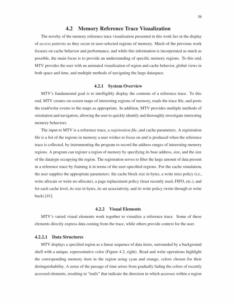
36
4.2 Memory Reference Trace VisualizationThe novelty of the memory reference trace visualization presented in this work lies in the display
of access patterns as they occur in user-selected regions of memory. Much of the previous work
focuses on cache behavior and performance, and while this information is incorporated as much as
possible, the main focus is to provide an understanding of specific memory regions. To this end,
MTV provides the user with an animated visualization of region and cache behavior, global views in
both space and time, and multiple methods of navigating the large dataspace.
4.2.1 System OverviewMTV’s fundamental goal is to intelligibly display the contents of a reference trace. To this
end, MTV creates on-screen maps of interesting regions of memory, reads the trace file, and posts
the read/write events to the maps as appropriate. In addition, MTV provides multiple methods of
orientation and navigation, allowing the user to quickly identify and thoroughly investigate interesting
memory behaviors.
The input to MTV is a reference trace, a registration file, and cache parameters. A registration
file is a list of the regions in memory a user wishes to focus on and is produced when the reference
trace is collected, by instrumenting the program to record the address ranges of interesting memory
regions. A program can register a region of memory by specifying its base address, size, and the size
of the datatype occupying the region. The registration serves to filter the large amount of data present
in a reference trace by framing it in terms of the user-specified regions. For the cache simulation,
the user supplies the appropriate parameters: the cache block size in bytes, a write miss policy (i.e.,
write allocate or write no-allocate), a page replacement policy (least recently used, FIFO, etc.), and
for each cache level, its size in bytes, its set associativity, and its write policy (write through or write
back) [41].
4.2.2 Visual ElementsMTV’s varied visual elements work together to visualize a reference trace. Some of these
elements directly express data coming from the trace, while others provide context for the user.
4.2.2.1 Data StructuresMTV displays a specified region as a linear sequence of data items, surrounded by a background
shell with a unique, representative color (Figure 4.2, right). Read and write operations highlight
the corresponding memory item in the region using cyan and orange, colors chosen for their
distinguishability. A sense of the passage of time arises from gradually fading the colors of recently
accessed elements, resulting in “trails” that indicate the direction in which accesses within a region
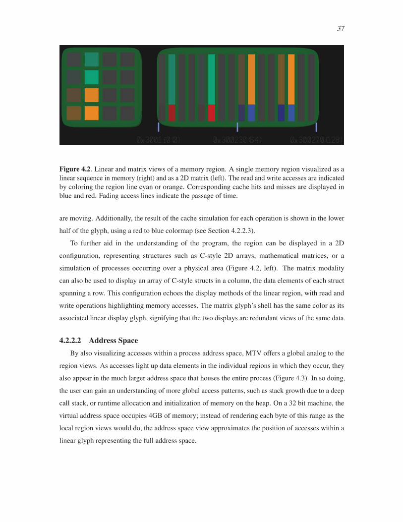
37
Figure 4.2. Linear and matrix views of a memory region. A single memory region visualized as a
linear sequence in memory (right) and as a 2D matrix (left). The read and write accesses are indicated
by coloring the region line cyan or orange. Corresponding cache hits and misses are displayed in
blue and red. Fading access lines indicate the passage of time.
are moving. Additionally, the result of the cache simulation for each operation is shown in the lower
half of the glyph, using a red to blue colormap (see Section 4.2.2.3).
To further aid in the understanding of the program, the region can be displayed in a 2D
configuration, representing structures such as C-style 2D arrays, mathematical matrices, or a
simulation of processes occurring over a physical area (Figure 4.2, left). The matrix modality
can also be used to display an array of C-style structs in a column, the data elements of each struct
spanning a row. This configuration echoes the display methods of the linear region, with read and
write operations highlighting memory accesses. The matrix glyph’s shell has the same color as its
associated linear display glyph, signifying that the two displays are redundant views of the same data.
4.2.2.2 Address SpaceBy also visualizing accesses within a process address space, MTV offers a global analog to the
region views. As accesses light up data elements in the individual regions in which they occur, they
also appear in the much larger address space that houses the entire process (Figure 4.3). In so doing,
the user can gain an understanding of more global access patterns, such as stack growth due to a deep
call stack, or runtime allocation and initialization of memory on the heap. On a 32 bit machine, the
virtual address space occupies 4GB of memory; instead of rendering each byte of this range as the
local region views would do, the address space view approximates the position of accesses within a
linear glyph representing the full address space.
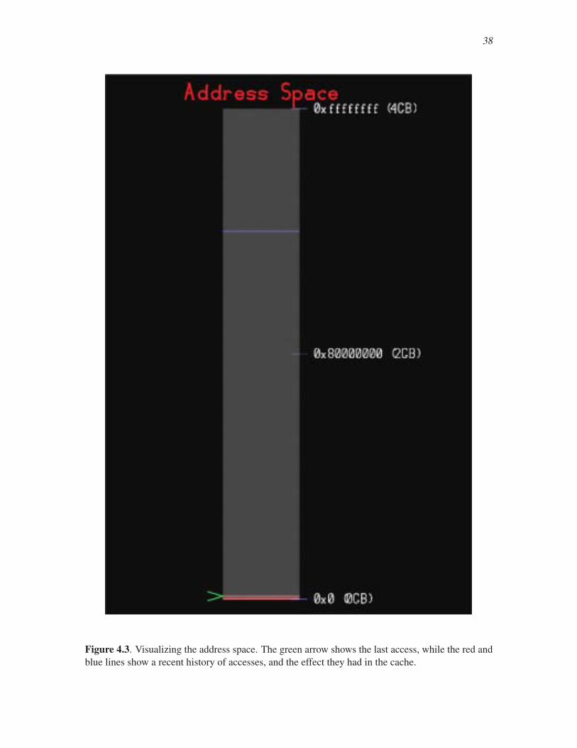
38
Figure 4.3. Visualizing the address space. The green arrow shows the last access, while the red and
blue lines show a recent history of accesses, and the effect they had in the cache.
39
4.2.2.3 Cache ViewIn addition to displaying a trace’s access patterns, MTV also performs cache simulation with
each reference record and displays the results in a schematic view of the cache. As the varying cache
miss rate serves as an indicator of memory performance, the cache view serves to connect memory
access patterns to a general measure of performance. By showing how the cache is affected by a
piece of code, MTV allows the user to understand what might be causing problematic performance.
The visualization of the cache is similar to that of linear regions with cache blocks shown in a
linear sequence surrounded by a colored shell (Figure 4.4). The cache is composed of multiple levels,
labeled L1 (the smallest, fastest level) through Ln (the largest, slowest level). The color of the upper
portion of the cache blocks in each level corresponds to the identifying color of the region which
last accessed that block, or a neutral color if the address does not belong to any of the user-declared
regions. The cache hit/miss status is indicated in the bottom portion of the memory blocks by a color
ranging from blue to red—blue for a hit to L1, red for a cache miss to main memory, and a blend
between blue and red for hits to levels slower than L1. To emphasize the presence of data from a
particular region in the cache, lines are also drawn between the address in the region view and the
affected blocks in the cache. Finally, the shells of each cache level reflect the cache temperature: the
warmer the temperature, the brighter the shell color.
4.2.3 Orientation and NavigationCombining a cache simulation with the tracking of memory access patterns creates a large,
possibly overwhelming amount of data. Reducing the visualized data to only important features,
providing useful navigation techniques, as well as relating events in the trace to source code is very
important to having a useful tool.
4.2.3.1 Memory System OrientationThe first step in managing the large dataset is to let the user filter the data by registering specific
memory regions (for example, program data structures) to visualize. During instrumentation, there is
no limit on the number of memory regions that can be specified, although in visualization, the screen
space taken by each region becomes a limitation. To ease this problem, the user is given the freedom
to move the regions anywhere on the screen during visualization. Clicking on a individual region
makes that region active, which brings that region to the forefront, and lines that relate the memory
locations of that region to locations in the cache are drawn (Figure 4.3, right).
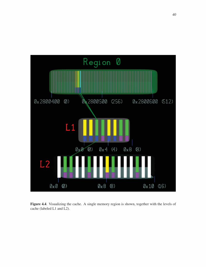
40
Figure 4.4. Visualizing the cache. A single memory region is shown, together with the levels of
cache (labeled L1 and L2).
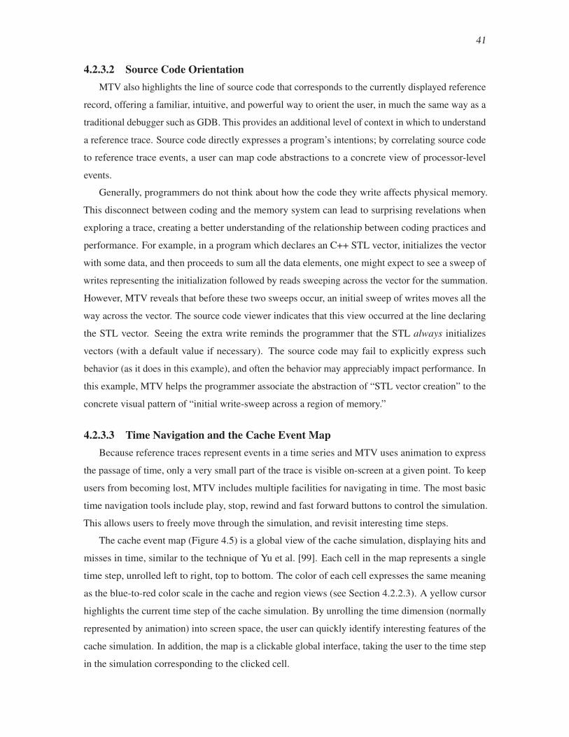
41
4.2.3.2 Source Code OrientationMTV also highlights the line of source code that corresponds to the currently displayed reference
record, offering a familiar, intuitive, and powerful way to orient the user, in much the same way as a
traditional debugger such as GDB. This provides an additional level of context in which to understand
a reference trace. Source code directly expresses a program’s intentions; by correlating source code
to reference trace events, a user can map code abstractions to a concrete view of processor-level
events.
Generally, programmers do not think about how the code they write affects physical memory.
This disconnect between coding and the memory system can lead to surprising revelations when
exploring a trace, creating a better understanding of the relationship between coding practices and
performance. For example, in a program which declares an C++ STL vector, initializes the vector
with some data, and then proceeds to sum all the data elements, one might expect to see a sweep of
writes representing the initialization followed by reads sweeping across the vector for the summation.
However, MTV reveals that before these two sweeps occur, an initial sweep of writes moves all the
way across the vector. The source code viewer indicates that this view occurred at the line declaring
the STL vector. Seeing the extra write reminds the programmer that the STL always initializes
vectors (with a default value if necessary). The source code may fail to explicitly express such
behavior (as it does in this example), and often the behavior may appreciably impact performance. In
this example, MTV helps the programmer associate the abstraction of “STL vector creation” to the
concrete visual pattern of “initial write-sweep across a region of memory.”
4.2.3.3 Time Navigation and the Cache Event MapBecause reference traces represent events in a time series and MTV uses animation to express
the passage of time, only a very small part of the trace is visible on-screen at a given point. To keep
users from becoming lost, MTV includes multiple facilities for navigating in time. The most basic
time navigation tools include play, stop, rewind and fast forward buttons to control the simulation.
This allows users to freely move through the simulation, and revisit interesting time steps.
The cache event map (Figure 4.5) is a global view of the cache simulation, displaying hits and
misses in time, similar to the technique of Yu et al. [99]. Each cell in the map represents a single
time step, unrolled left to right, top to bottom. The color of each cell expresses the same meaning
as the blue-to-red color scale in the cache and region views (see Section 4.2.2.3). A yellow cursor
highlights the current time step of the cache simulation. By unrolling the time dimension (normally
represented by animation) into screen space, the user can quickly identify interesting features of the
cache simulation. In addition, the map is a clickable global interface, taking the user to the time step
in the simulation corresponding to the clicked cell.

42
����������������� ��������
������� �����������������������������������������������
��������������������������������������
Figure 4.5. Cache event map. The cache event map provides a global view of the cache simulation
by showing the cache status for each time step, and a clickable time navigation interface. The time
dimension starts at the upper left of the map and proceeds across the image in English text order.
4.3 ExamplesThe following examples demonstrate how MTV can be used to illuminate performance issues
resulting from code behavior. For the first example, a simple cache is simulated: The block size
is 16 bytes (large enough to store four single-precision floating point numbers); L1 is two-way
set associative, with four cache blocks; L2 is eight-way set associative, with eight cache blocks.
In the second example, the cache has the same block size but twice as many blocks in each level.
These caches simplify the demonstrations, but much larger caches can be used in practice. The third
example simulates the cache found in a PowerMac G5. It has a block size of 128 bytes; the 32K L1
is two-way set associative, and the 512K L2 is eight-way set associative.
4.3.1 Loop InterchangeA common operation in scientific programs is to make a pass through an array of data and do
something with each data item. Often, the data are organized in multidimensional arrays; in such
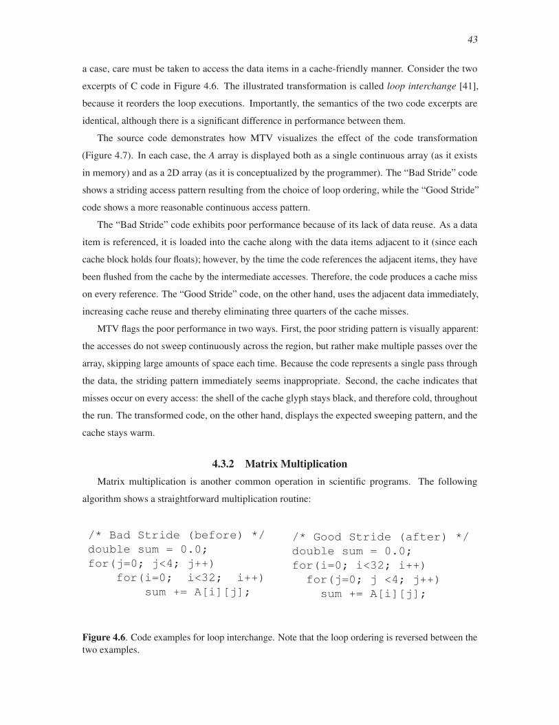
43
a case, care must be taken to access the data items in a cache-friendly manner. Consider the two
excerpts of C code in Figure 4.6. The illustrated transformation is called loop interchange [41],
because it reorders the loop executions. Importantly, the semantics of the two code excerpts are
identical, although there is a significant difference in performance between them.
The source code demonstrates how MTV visualizes the effect of the code transformation
(Figure 4.7). In each case, the A array is displayed both as a single continuous array (as it exists
in memory) and as a 2D array (as it is conceptualized by the programmer). The “Bad Stride” code
shows a striding access pattern resulting from the choice of loop ordering, while the “Good Stride”
code shows a more reasonable continuous access pattern.
The “Bad Stride” code exhibits poor performance because of its lack of data reuse. As a data
item is referenced, it is loaded into the cache along with the data items adjacent to it (since each
cache block holds four floats); however, by the time the code references the adjacent items, they have
been flushed from the cache by the intermediate accesses. Therefore, the code produces a cache miss
on every reference. The “Good Stride” code, on the other hand, uses the adjacent data immediately,
increasing cache reuse and thereby eliminating three quarters of the cache misses.
MTV flags the poor performance in two ways. First, the poor striding pattern is visually apparent:
the accesses do not sweep continuously across the region, but rather make multiple passes over the
array, skipping large amounts of space each time. Because the code represents a single pass through
the data, the striding pattern immediately seems inappropriate. Second, the cache indicates that
misses occur on every access: the shell of the cache glyph stays black, and therefore cold, throughout
the run. The transformed code, on the other hand, displays the expected sweeping pattern, and the
cache stays warm.
4.3.2 Matrix MultiplicationMatrix multiplication is another common operation in scientific programs. The following
algorithm shows a straightforward multiplication routine:
/* Bad Stride (before) */ double sum = 0.0; for(j=0; j<4; j++) for(i=0; i<32; i++) sum += A[i][j];
/* Good Stride (after) */ double sum = 0.0;for(i=0; i<32; i++) for(j=0; j <4; j++) sum += A[i][j];
Figure 4.6. Code examples for loop interchange. Note that the loop ordering is reversed between the
two examples.

44
Figure 4.7. Comparing access orders for a two-dimensional array. Striding a two-dimensional array
in different orders produces a marked difference in performance.
for(i=0; i<N; i++)
for(j=0; j<N; j++){
r = 0.0;
for(k=0; k<N; k++)
r += Y[i*N+k] * Z[k*N+j];
X[i*N+j] = r;
}
MTV shows the familiar pattern associated with matrix multiplication by the order in which the
accesses to the X , Y , and Z matrices occur (Figure 4.8, top). The troublesome access pattern in this
reference trace occurs in matrix Z, which must be accessed column-by-column because of the way
the algorithm runs.
In order to rectify the access pattern, the programmer may transform the code to store the
transpose of matrix Z. Then, to perform the proper multiplication, Z would have to be accessed in
row-major order, eliminating the problematic access pattern. When certain matrices always appear
first in a matrix product and others always appear second, one possible solution is to store matrices
of the former type in row-major order and those of the latter type in column-major order. In this
example, the visual patterns encoded in the trace (Figure 4.8, top) suggested a code transformation.
This transformation also suggests a new abstraction of left- vs. right-multiplicand matrices that may
help to increase the performance of codes relying heavily on matrix multiplication. A more general
solution to improving matrix multiplication is widely known as matrix blocking, in which algorithms
operate on small submatrices that fit into cache, accumulating the correct answer by making several
passes (Figure 4.8, bottom).

45
Figure 4.8. Comparing naive and blocked matrix multiplication. Naive matrix multiply (top) and
blocked matrix multiply (bottom).
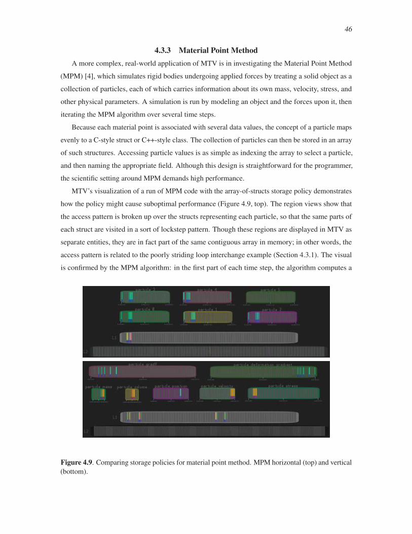
46
4.3.3 Material Point MethodA more complex, real-world application of MTV is in investigating the Material Point Method
(MPM) [4], which simulates rigid bodies undergoing applied forces by treating a solid object as a
collection of particles, each of which carries information about its own mass, velocity, stress, and
other physical parameters. A simulation is run by modeling an object and the forces upon it, then
iterating the MPM algorithm over several time steps.
Because each material point is associated with several data values, the concept of a particle maps
evenly to a C-style struct or C++-style class. The collection of particles can then be stored in an array
of such structures. Accessing particle values is as simple as indexing the array to select a particle,
and then naming the appropriate field. Although this design is straightforward for the programmer,
the scientific setting around MPM demands high performance.
MTV’s visualization of a run of MPM code with the array-of-structs storage policy demonstrates
how the policy might cause suboptimal performance (Figure 4.9, top). The region views show that
the access pattern is broken up over the structs representing each particle, so that the same parts of
each struct are visited in a sort of lockstep pattern. Though these regions are displayed in MTV as
separate entities, they are in fact part of the same contiguous array in memory; in other words, the
access pattern is related to the poorly striding loop interchange example (Section 4.3.1). The visual
is confirmed by the MPM algorithm: in the first part of each time step, the algorithm computes a
Figure 4.9. Comparing storage policies for material point method. MPM horizontal (top) and vertical
(bottom).

47
momentum value by looking at the mass and velocity of each particle (in Figure 4.9, top, the single
lit value at the left of each region is the mass value, while the three lit values to the right of the mass
comprise the velocity). In fact, much of the MPM algorithm operates this way: values of the same
type are needed at roughly the same time, rather than each particle being processed in whole, one at
a time.
MTV demonstrates a feature of the MPM implementation that is normally hidden: the chosen
storage policy implies a necessarily noncontiguous access pattern. The simplest way to rearrange the
storage is to use parallel arrays instead of an array of structs, so that all the masses are found in one
array, the velocities in another, and so on. Grouping similar values together gives the algorithm a
better chance of finding the next values it needs nearby. This storage policy results in a more coherent
access pattern, and higher overall performance (Figure 4.9, bottom).
This particular observation and the simple solution it suggests are both tied to our understanding
of the algorithm. By making even more careful observations, it should be possible to come up with a
hybrid storage policy that respects more of the algorithm’s idiosyncrasies and achieves higher perfor-
mance. The example also stresses the value of abstraction, and in particular, the value of separating
interfaces from implementations. By having an independent interface to the particle data (consisting
of functions or methods with signatures like double getMass(int particleId);), the
data storage policy is hidden appropriately and can vary freely for performance or other concerns.
4.4 ConclusionsThe gap between processor and memory performance, and the rising number of cores per chip,
will be a persistent problem for memory-bound applications until major changes are made in the
memory paradigm. This chapter has described the Memory Trace Visualizer, a tool that is designed to
explicitly examine the interaction between a program and memory through visualization of detailed
reference traces. MTV provides a technique for the rich yet inscrutable reference trace data by
offering visual metaphors for abstract memory operations, leading to a deeper understanding of
memory usage and therefore opportunities for optimization.
MTV provides a straightforward, architectural view of memory access behavior, bringing some
basic insights in program behavior as described here. In the next chapter, these ideas are extended in
a different, more abstract approach, featuring richer visual metaphors and focusing more on the cache
itself, while also striving to maintain the visualization of fundamental access patterns, as introduced
in MTV.
CHAPTER 5
ABSTRACT VISUALIZATION OF MEMORY
REFERENCE TRACES WITH WAXLAMP
In contrast to the straightforward, few-frills visualization approach offered by MTV, this chapter
describes Waxlamp, a more abstract approach to reference trace visualization that focuses on the
cache, its contents, and how they change as a function of time. The focus on the internal structure
of the cache brings new insights, including diagnosis for certain kinds of cache behavior faults that
would be very difficult to see using other approaches. The Waxlamp approach is abstract in that it
also suggests a general recipe for building visualization schemata for other kinds of performance
data, allowing for a flexible approach to thinking about such data.
5.1 IntroductionIn optimizing program performance, one common analysis technique is to track cache activity
within an application. This information is usually provided by profilers or other special-purpose
software for very coarse time granularity. At best, cache performance is provided for blocks of code
or individual functions. At worst, these results are captured for an entire application’s execution.
This provides only a global view of performance and limits the ability to intuitively understand
performance. An alternative to this coarse granularity is to generate a memory reference trace, which
can then be run through a cache simulator to produce a fine-grained approximation of the software’s
actual cache performance.
The biggest challenge when using this approach is sifting through the volume of data produced.
Even simple applications can produce millions of references, yet this data contains valuable
information that needs to be extracted to better understand program performance. The use of
statistical methods or averaging simply produces a coarse understanding of software performance,
forgoing the detail available in the trace. Static analysis of memory behavior is also possible [10],
but limited only to cases where the program behavior can be deduced at compile time.
The Waxlamp system proposes to address these problems by visualizing the simulated cache
and the reference trace, allowing developers to see their software with fine-grained detail, and bring

49
their experience and intuition to bear on understanding software memory performance. Waxlamp
accomplishes this by providing an abstract visualization of the cache as the reference trace plays
through it.
The goal of Waxlamp is to provide an intuitive understanding of how the computer hardware
affects software performance, without the need to know or understand every feature of the hardware
itself. The resulting visualizations correspond to an intuitive understanding of how caches work, yet
are able to convey cache activity that may be difficult to envision or else are surprising in some way.
The approach is not a replacement for other conventional approaches, but rather an additional tool
that can assist in software analysis.
Figure 5.1 shows four example images of Waxlamp visualizing different versions of the matrix
multiply algorithm. Memory locations, represented by point glyphs, are placed on concentric rings
based upon their cache residency. Lighter-colored, ghost glyphs are placed in the higher levels of
cache (and the main memory region) to indicate duplication of data through the levels of the memory
hierarchy. The outermost ring contains items in main memory, the middle ring contains items in the
level 2 (L2) cache, and the innermost ring contains items in the level 1 (L1) cache. The visualization
provides an intuitive understanding about how memory is used and evicted from the cache. As
locations are referenced, their glyphs move to the center of the visualization, and as they age (and are
eventually evicted), they are pushed out towards the next concentric ring.
Waxlamp is inspired by organic visualization [32], an approach that imbues the visual elements
with behavioral rules that allow them to self-organize into meaningful visual structures, much as
individual cells are able to work together to constitute a whole organism. Codeswarm [63] is an
example of the technique as applied to software visualization, in which source code repository
data directs visual elements representing files and developers to form groups according to tight
relationships between them. For instance, frequent committers associate into circles with their
working files. Motion, proximity, color, and size all work together to express the important
relationships between the participants. Waxlamp is inspired by systems such as Codeswarm, as such
organic visualization systems are able to handle many visual elements by allowing them to aggregate
automatically into higher-level structures—such as levels of a cache and semantically delineated
regions of memory—so that their sheer volume does not obscure the insights they try to transmit.
Compared to this more organic visualization behavior, MTV (Chapter 4) addresses the same problem
of visualizing reference traces, but in a more regimented, litral way. Concrete access patterns are
more visible in MTV, while Waxlamp is better able to show cache dynamics and data motion.

50
(a) (b) (c) (d)
Figure 5.1. Matrix multiply in various incarnations: (a) Standard 16×16 matrix multiply. (b)
Transposed-storage 16×16 matrix multiply. (c) 16×16 matrix multiply with 4×4 blocking. (d)
12×12 matrix multiply with 4×4 blocking. The standard algorithm shows good cache behavior for
the left-hand matrix but poor behavior for the right-hand matrix. One solution is to operate on a
transposed-storage version of the right-hand matrix, which results in better cache behavior, but a
loss of generality in the allowed matrix operations. A common solution between the two is matrix
blocking, in which submatrices are operated on to accumulate the final result piece by piece. By
operating on small submatrices that fit into the cache, the cache performance of the multiply improves
while keeping the generality of the standard matrix multiplication algorithm.
5.2 Visualizing Reference TracesThis section describes the design of Waxlamp, focusing on the nature and usage of individual
visual channels. In particular, time scales in each channel are distinguished by “frequency,” reflecting
the time scales over which changes in visual qualities tend to persist. Channels engage a low
frequency when visual elements exhibit a longer-term, stable behavior, and a high frequency when
they change rapidly. By way of example, consider the position of a data glyph—the low-frequency
behavior is to settle into a position within a cache level or main memory; the high-frequency behavior
is to move from one area to another in response to a cache level eviction event. Generally speaking,
low-frequency qualities are used to establish baselines or express average behaviors over a long time
period, reserving high-frequency qualities to reflect sudden changes in state, or very important events
that need to draw the viewer’s attention.
In broad strokes, the visualization system consists of a structural layout representing the levels
of cache, and main memory, over which data glyphs, representing individual addressable pieces of
memory, move according to behavioral rules. The positions of these glyphs encode their presence in
one or more levels of cache.
5.2.1 Structured Cache LayoutThe data glyphs occupy a structured visual space representing the machine architecture under
consideration (Figure 5.2, left). Because locality is so important in understanding cache and memory
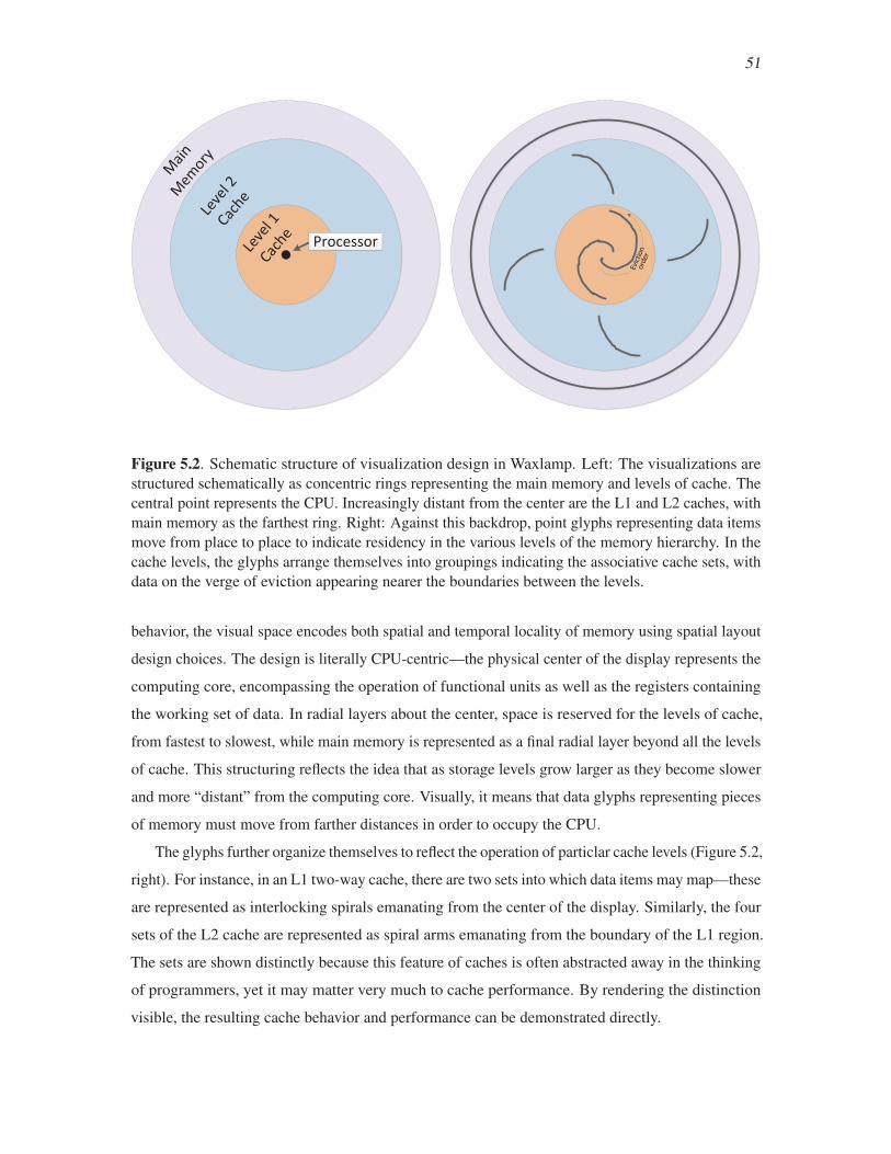
51
Main
M
emory
Leve
l 2
Cache
Leve
l 1
Cache Processor
Evict
ion
orde
r
Figure 5.2. Schematic structure of visualization design in Waxlamp. Left: The visualizations are
structured schematically as concentric rings representing the main memory and levels of cache. The
central point represents the CPU. Increasingly distant from the center are the L1 and L2 caches, with
main memory as the farthest ring. Right: Against this backdrop, point glyphs representing data items
move from place to place to indicate residency in the various levels of the memory hierarchy. In the
cache levels, the glyphs arrange themselves into groupings indicating the associative cache sets, with
data on the verge of eviction appearing nearer the boundaries between the levels.
behavior, the visual space encodes both spatial and temporal locality of memory using spatial layout
design choices. The design is literally CPU-centric—the physical center of the display represents the
computing core, encompassing the operation of functional units as well as the registers containing
the working set of data. In radial layers about the center, space is reserved for the levels of cache,
from fastest to slowest, while main memory is represented as a final radial layer beyond all the levels
of cache. This structuring reflects the idea that as storage levels grow larger as they become slower
and more “distant” from the computing core. Visually, it means that data glyphs representing pieces
of memory must move from farther distances in order to occupy the CPU.
The glyphs further organize themselves to reflect the operation of particlar cache levels (Figure 5.2,
right). For instance, in an L1 two-way cache, there are two sets into which data items may map—these
are represented as interlocking spirals emanating from the center of the display. Similarly, the four
sets of the L2 cache are represented as spiral arms emanating from the boundary of the L1 region.
The sets are shown distinctly because this feature of caches is often abstracted away in the thinking
of programmers, yet it may matter very much to cache performance. By rendering the distinction
visible, the resulting cache behavior and performance can be demonstrated directly.

52
As mentioned above, the placement of the cache sets reflects their progressive “distance” from
the CPU core; within each cache set representation, distance also encodes the eviction order, with
glyphs that are about to be evicted from the cache positioned further away from the center, on the
border with the slower cache level to which they will be sent.
A common cache design uses the “least recently used” (LRU) heuristic in deciding which cache
block should be evicted when a new block arrives. Under an LRU block replacement strategy,
distance from the center of the display can also be taken to encode time, so that glyphs that are more
“stale” (i.e., have not been accessed for a long time) tend to appear further from the center. This
placement rule renders certain access behaviors clearly visible. For instance, a common memory
access pattern is that of array initialization, in which a newly created array must have its entries all
set to some base value (Figure 5.3). Tracking a single data item d through the cache would reveal
that at some point in time, it is brought into L1, where it is initialized. As subsequent data items are
processed, d becomes older in L1, so it progressively moves further away along its spiral arm. When
it reaches the end of the spiral, and yet another block is brought into L1, it is evicted to L2, where a
similar process occurs, finally ejecting d back to its original home in main memory. Because time is,
in this way, encoded as distance from the center, d moves along a radial path as it ages, eventually
leaving the cache altogether. The visual pattern makes clear how the lack of reuse of d makes it both
“older” and pushes it “far away” at the same time.
Figure 5.3. Visualizing array initialization in Waxlamp at three points in time. The red streak lines
indicate cache misses for references to the green array. The data comes into L1 and is initialized
with a series of write operations. As the next batch of data comes in, the initialized data becomes
“stale” and moves slowly first out of L1 to L2, then out of L2 back into main memory. The bundle of
red cache miss lines is seen to rotate through the array as the array items stream through, visually
characterizing this pattern of access.
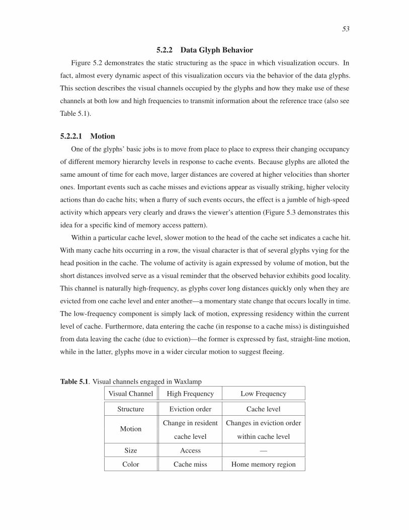
53
5.2.2 Data Glyph BehaviorFigure 5.2 demonstrates the static structuring as the space in which visualization occurs. In
fact, almost every dynamic aspect of this visualization occurs via the behavior of the data glyphs.
This section describes the visual channels occupied by the glyphs and how they make use of these
channels at both low and high frequencies to transmit information about the reference trace (also see
Table 5.1).
5.2.2.1 MotionOne of the glyphs’ basic jobs is to move from place to place to express their changing occupancy
of different memory hierarchy levels in response to cache events. Because glyphs are alloted the
same amount of time for each move, larger distances are covered at higher velocities than shorter
ones. Important events such as cache misses and evictions appear as visually striking, higher velocity
actions than do cache hits; when a flurry of such events occurs, the effect is a jumble of high-speed
activity which appears very clearly and draws the viewer’s attention (Figure 5.3 demonstrates this
idea for a specific kind of memory access pattern).
Within a particular cache level, slower motion to the head of the cache set indicates a cache hit.
With many cache hits occurring in a row, the visual character is that of several glyphs vying for the
head position in the cache. The volume of activity is again expressed by volume of motion, but the
short distances involved serve as a visual reminder that the observed behavior exhibits good locality.
This channel is naturally high-frequency, as glyphs cover long distances quickly only when they are
evicted from one cache level and enter another—a momentary state change that occurs locally in time.
The low-frequency component is simply lack of motion, expressing residency within the current
level of cache. Furthermore, data entering the cache (in response to a cache miss) is distinguished
from data leaving the cache (due to eviction)—the former is expressed by fast, straight-line motion,
while in the latter, glyphs move in a wider circular motion to suggest fleeing.
Table 5.1. Visual channels engaged in Waxlamp
Visual Channel High Frequency Low Frequency
Structure Eviction order Cache level
MotionChange in resident Changes in eviction order
cache level within cache level
Size Access —
Color Cache miss Home memory region
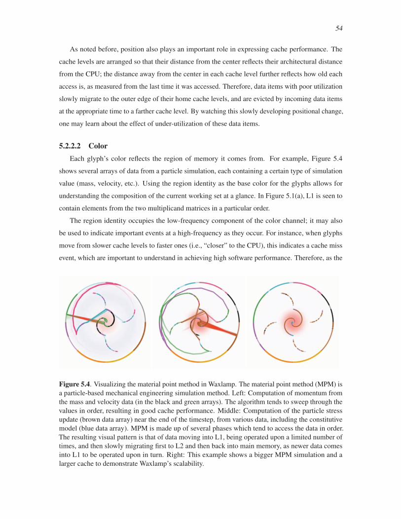
54
As noted before, position also plays an important role in expressing cache performance. The
cache levels are arranged so that their distance from the center reflects their architectural distance
from the CPU; the distance away from the center in each cache level further reflects how old each
access is, as measured from the last time it was accessed. Therefore, data items with poor utilization
slowly migrate to the outer edge of their home cache levels, and are evicted by incoming data items
at the appropriate time to a farther cache level. By watching this slowly developing positional change,
one may learn about the effect of under-utilization of these data items.
5.2.2.2 ColorEach glyph’s color reflects the region of memory it comes from. For example, Figure 5.4
shows several arrays of data from a particle simulation, each containing a certain type of simulation
value (mass, velocity, etc.). Using the region identity as the base color for the glyphs allows for
understanding the composition of the current working set at a glance. In Figure 5.1(a), L1 is seen to
contain elements from the two multiplicand matrices in a particular order.
The region identity occupies the low-frequency component of the color channel; it may also
be used to indicate important events at a high-frequency as they occur. For instance, when glyphs
move from slower cache levels to faster ones (i.e., “closer” to the CPU), this indicates a cache miss
event, which are important to understand in achieving high software performance. Therefore, as the
Figure 5.4. Visualizing the material point method in Waxlamp. The material point method (MPM) is
a particle-based mechanical engineering simulation method. Left: Computation of momentum from
the mass and velocity data (in the black and green arrays). The algorithm tends to sweep through the
values in order, resulting in good cache performance. Middle: Computation of the particle stress
update (brown data array) near the end of the timestep, from various data, including the constitutive
model (blue data array). MPM is made up of several phases which tend to access the data in order.
The resulting visual pattern is that of data moving into L1, being operated upon a limited number of
times, and then slowly migrating first to L2 and then back into main memory, as newer data comes
into L1 to be operated upon in turn. Right: This example shows a bigger MPM simulation and a
larger cache to demonstrate Waxlamp’s scalability.
55
glyphs move to the L1 cache in response to such an event, they flash red momentarily to indicate
their involvement in the cache miss event.
5.2.2.3 SizeAlong with color, the size of the glyphs makes up their basic visual composition. The data glyphs
all have an equal baseline size (i.e., the low-frequency size channel empty) in order to emphasize the
relative composition of the cache levels without singling out any particular data items.
The high-frequency size channel is used to redundantly encode an access to a particular data item.
When a data item is accessed, it pulses larger momentarily, with the effect of highlighting it among
all the data items present in the cache level along with it. When the data item is not already present in
the L1 level, its pulsation can be seen as it moves into L1 in response to the cache miss event, once
again highlighting the important event (in this case, the pulsation redundantly strengthens the red
glow as discussed above).
5.2.3 Time-Lapse ModeMemory reference traces can be very large; as such, visualizations produced from them can be
intractably long to observe. One option would be to simply speed up the visualization by increasing
the speed of trace playback and glyph motion. This approach works until the speed becomes so high
that glyph motion is no longer visible.
To address this limitation, several timesteps can be compressed into a single animation frame,
encoding the changes in glyph positions through time by using pathlines. First, a fast forward speed
is set (e.g., 2×, 4×, etc.), indicating the number of animation frames to skip in visualization. The
positions of glyphs are calculated for those skipped frames, and a pathline is used to connect the
glyph positions at those intermediate times. When the time-compressed frames are played at a normal
speed, simulation time appears to have sped up dramatically, yet the pathlines keep the sense of
evolving time coherent.
The pathlines can be controllably extended further into history as desired. Figure 5.5 shows
four different settings for the tail length for the same time step. Increasing the tail length shows
more events, but also tends obscure individual events—the tradeoff can be managed by the user
interactively. Transparency in the pathlines indicates age, older events appearing more transparent,
while newer events appear opaque. The time-lapse view therefore shows higher-order temporal
patterns in addition to managing the commonly long time scales present in most reference traces.

56
(a) No history (b) 16 frames (c) 32 frames (d) 64 frames
Figure 5.5. History pathlines in Waxlamp. These four images are of the exact same simulation time,
varying only in the amount of history accumulated into the fading trails: (a) shows only the current
animation frame, with no sense of history. (b) shows the last 16 frames, which indicate that L1 hits
have been taking place in the recent past. In (c) there is evidence of a recent cache miss, and an
associated eviction event, while (d) shows these same events in heavier detail. Note that while the
same set of events is visible in (c) and (d), the longer history trail in (d) tends to obscure the L1
activity that is clearer in (b). By providing an interactive control for this feature, the user can select
the amount of history that is appropriate for the current visual analysis task.
5.2.4 Summary ViewsThe structured layout also provides for displaying a general quantity computed from the trace as a
whole, allowing, for example, statistical information about the trace to be included in the display. The
computed value is displayed in a soft, colormapped disk behind the areas reserved for the cache levels.
In the examples, the “cache temperature” is computed, a measure of the proportion of transactions in
each cache level resulting in a hit. More precisely, each reference trace record causes a change in the
cache: each level may either hit, miss, or else be uninvolved in the transaction. These are assigned
scores (a negative value for a miss, a positive value for a hit, and zero for noninvolvement) which are
averaged over the last N reference trace records. The assigned scores may vary for different levels;
for example, the penalty for a miss is higher for the L1 cache, because once a cache line is loaded
into L1, it will have more of a chance to make heavy reuse of the data than a slower level would.
In each level, the cache temperature rises above zero when the volume of data reuse exceeds the
“break even” point, and falls below zero when there is not enough reuse. When a cache level sits idle
(because, for instance, faster levels are hitting at a high rate), its temperature gradually drifts back to
zero. The metaphor is that new data are cold, causing a drop in temperature, but accessing resident
data releases energy and raises the temperature. Between these extremes, sitting idle allows for the
temperature to return slowly to a neutral point.
The cache temperature is displayed as a glowing color behind the appropriate structural elements
of the display. A divergent colormap consisting of colors that naturally express relative temperatures
is used, running from white in the middle (the neutral color indicating no activity, or a balance of hits
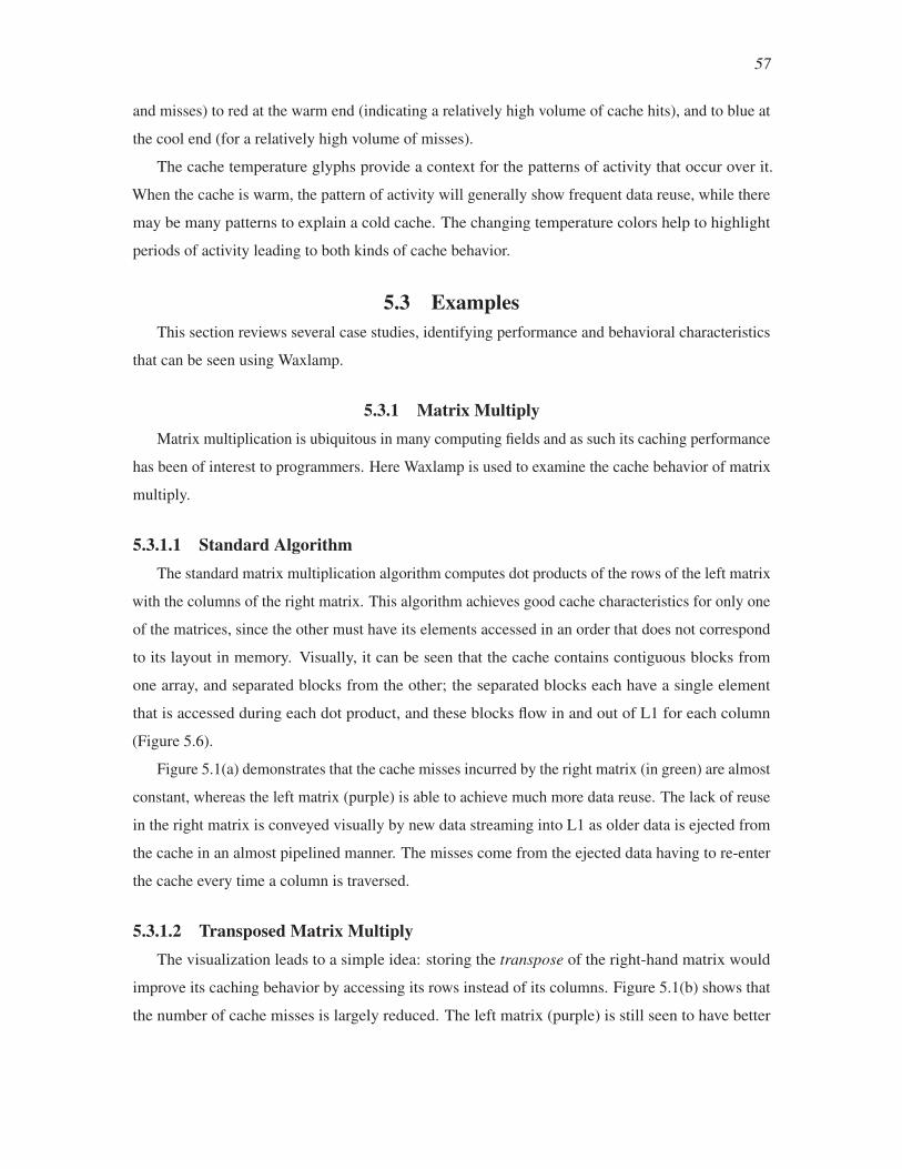
57
and misses) to red at the warm end (indicating a relatively high volume of cache hits), and to blue at
the cool end (for a relatively high volume of misses).
The cache temperature glyphs provide a context for the patterns of activity that occur over it.
When the cache is warm, the pattern of activity will generally show frequent data reuse, while there
may be many patterns to explain a cold cache. The changing temperature colors help to highlight
periods of activity leading to both kinds of cache behavior.
5.3 ExamplesThis section reviews several case studies, identifying performance and behavioral characteristics
that can be seen using Waxlamp.
5.3.1 Matrix MultiplyMatrix multiplication is ubiquitous in many computing fields and as such its caching performance
has been of interest to programmers. Here Waxlamp is used to examine the cache behavior of matrix
multiply.
5.3.1.1 Standard AlgorithmThe standard matrix multiplication algorithm computes dot products of the rows of the left matrix
with the columns of the right matrix. This algorithm achieves good cache characteristics for only one
of the matrices, since the other must have its elements accessed in an order that does not correspond
to its layout in memory. Visually, it can be seen that the cache contains contiguous blocks from
one array, and separated blocks from the other; the separated blocks each have a single element
that is accessed during each dot product, and these blocks flow in and out of L1 for each column
(Figure 5.6).
Figure 5.1(a) demonstrates that the cache misses incurred by the right matrix (in green) are almost
constant, whereas the left matrix (purple) is able to achieve much more data reuse. The lack of reuse
in the right matrix is conveyed visually by new data streaming into L1 as older data is ejected from
the cache in an almost pipelined manner. The misses come from the ejected data having to re-enter
the cache every time a column is traversed.
5.3.1.2 Transposed Matrix MultiplyThe visualization leads to a simple idea: storing the transpose of the right-hand matrix would
improve its caching behavior by accessing its rows instead of its columns. Figure 5.1(b) shows that
the number of cache misses is largely reduced. The left matrix (purple) is still seen to have better
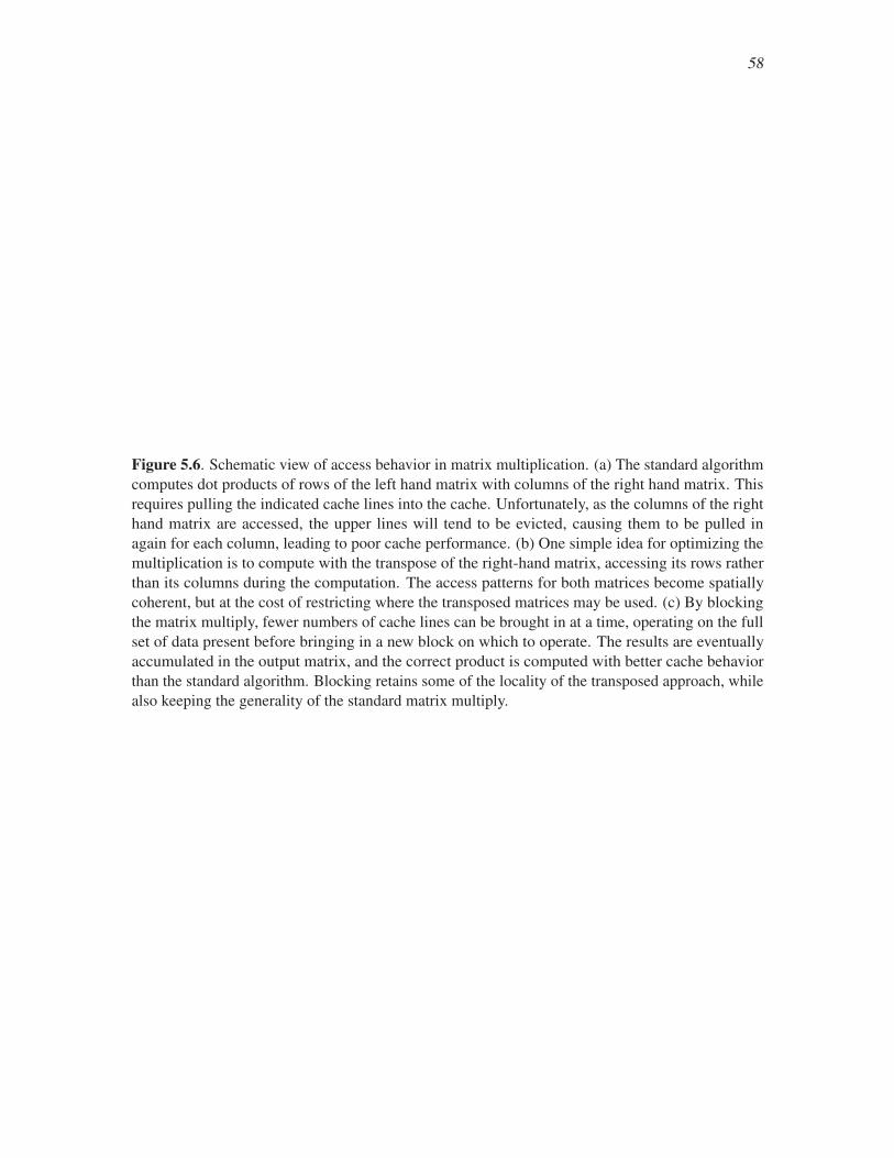
58
Figure 5.6. Schematic view of access behavior in matrix multiplication. (a) The standard algorithm
computes dot products of rows of the left hand matrix with columns of the right hand matrix. This
requires pulling the indicated cache lines into the cache. Unfortunately, as the columns of the right
hand matrix are accessed, the upper lines will tend to be evicted, causing them to be pulled in
again for each column, leading to poor cache performance. (b) One simple idea for optimizing the
multiplication is to compute with the transpose of the right-hand matrix, accessing its rows rather
than its columns during the computation. The access patterns for both matrices become spatially
coherent, but at the cost of restricting where the transposed matrices may be used. (c) By blocking
the matrix multiply, fewer numbers of cache lines can be brought in at a time, operating on the full
set of data present before bringing in a new block on which to operate. The results are eventually
accumulated in the output matrix, and the correct product is computed with better cache behavior
than the standard algorithm. Blocking retains some of the locality of the transposed approach, while
also keeping the generality of the standard matrix multiply.
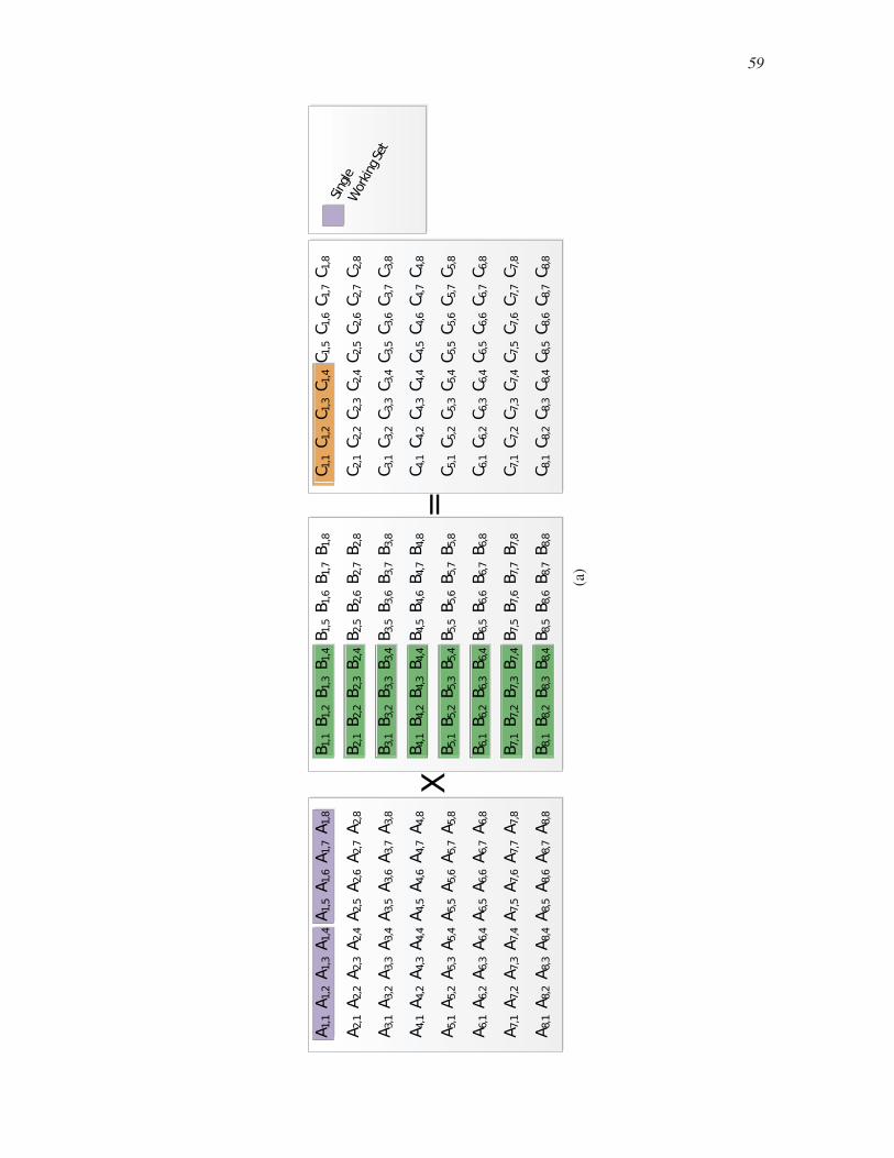
59
� ���� �
��� �
��� �
��� �
��� �
�� �
�� �
��
� ���� �
��� �
��� �
��� �
��� �
�� �
�� �
��
� ���� �
��� �
��� �
��� �
��� �
�� �
�� �
��
� ���� �
��� �
��� �
��� �
��� �
�� �
�� �
��
� ���� �
��� �
��� �
��� �
��� �
�� �
�� �
��
� ���
���
���
���
���
��
��
��
� ���
���
���
���
���
��
��
��
� ���� �
��� �
��� �
��� �
��� �
�� �
�� �
��
� ���� �
��� �
��� �
��� �
��� �
�� �
�� �
��
� ���� �
��� �
��� �
��� �
��� �
�� �
�� �
��
� ���� �
��� �
��� �
��� �
��� �
�� �
�� �
��
� ���� �
��� �
��� �
��� �
��� �
�� �
�� �
��
� ���� �
��� �
��� �
��� �
��� �
�� �
�� �
��
� ���
���
���
���
���
��
��
��
� ���
���
���
���
���
��
��
��
� ���� �
��� �
��� �
��� �
��� �
�� �
�� �
��
��� �
�� �
�� �
�� �
�� �
� �
� �
��
��� �
�� �
�� �
�� �
�� �
� �
� �
��
��� �
�� �
�� �
�� �
�� �
� �
� �
��
��� �
�� �
�� �
�� �
�� �
� �
� �
��
��� �
�� �
�� �
�� �
�� �
� �
� �
��
��
��
��
��
��
�
�
��
��
��
��
��
��
�
�
��
��� �
�� �
�� �
�� �
�� �
� �
� �
��
��
������
����������
(a)
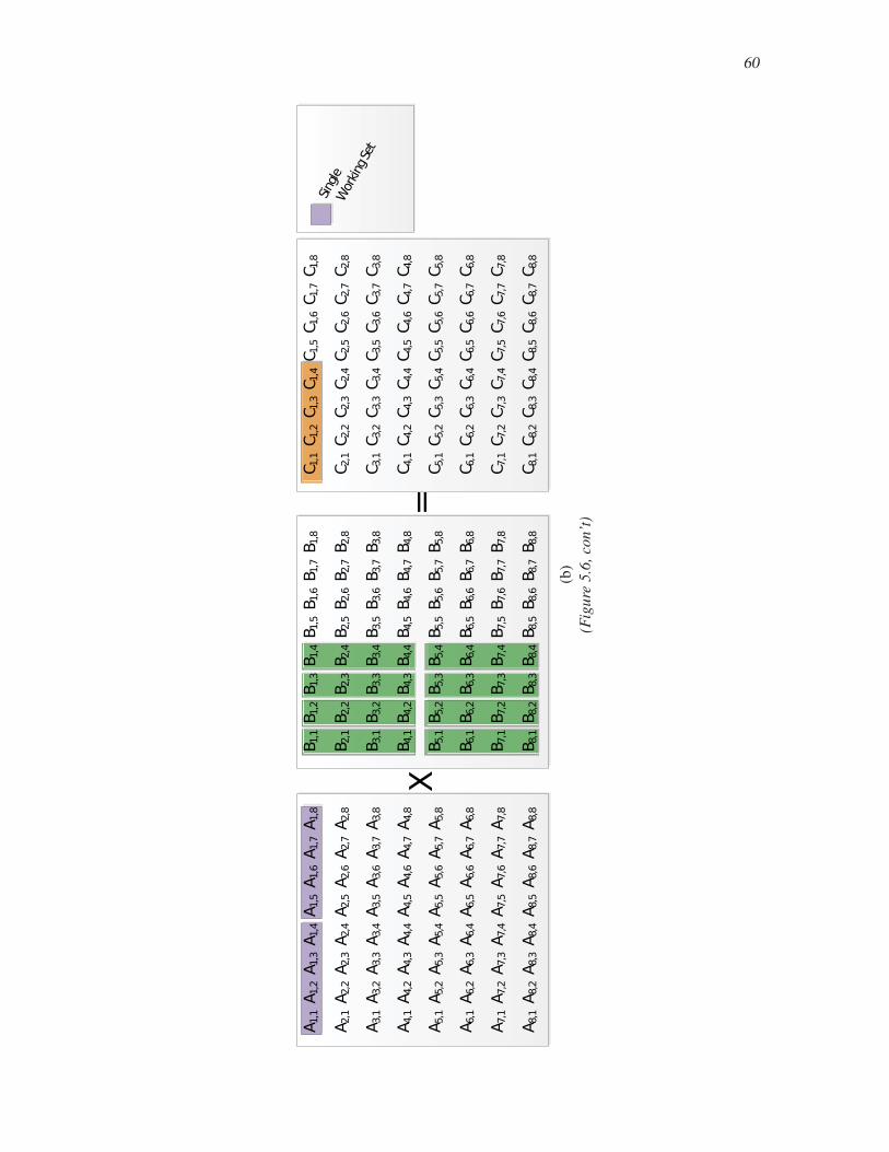
60
���������
�
� ���� �
��� �
��� �
��� �
��� �
��� �
��� �
��
� ���� �
��� �
��� �
��� �
��� �
��� �
��� �
��
� ���� �
��� �
��� �
��� �
��� �
��� �
��� �
��
� ���� �
��� �
��� �
��� �
��� �
��� �
��� �
��
� ���� �
��� �
��� �
��� �
��� �
��� �
��� �
��
� ���� �
��� �
��� �
��� �
��� �
��� �
��� �
��
� ���� �
��� �
��� �
��� �
��� �
��� �
��� �
��
� ���� �
��� �
��� �
��� �
��� �
��� �
��� �
��
� ���� �
��� �
��� �
��� �
��� �
��� �
��� �
��
� ���� �
��� �
��� �
��� �
��� �
��� �
��� �
��
� ���� �
��� �
��� �
��� �
��� �
��� �
��� �
��
� ���� �
��� �
��� �
��� �
��� �
��� �
��� �
��
� ���� �
��� �
��� �
��� �
��� �
��� �
��� �
��
� ���� �
��� �
��� �
��� �
��� �
��� �
��� �
��
� ���� �
��� �
��� �
��� �
��� �
��� �
��� �
��
� ���� �
��� �
��� �
��� �
��� �
��� �
��� �
��
��
����
�������
� ���� �
��� �
��� �
��� �
��� �
��� �
��� �
��
� ���� �
��� �
��� �
��� �
��� �
��� �
��� �
��
� ���� �
��� �
��� �
��� �
��� �
��� �
��� �
��
� ���� �
��� �
��� �
��� �
��� �
��� �
��� �
��
� ���� �
��� �
��� �
��� �
��� �
��� �
��� �
��
� ���� �
��� �
��� �
��� �
��� �
��� �
��� �
��
� ���� �
��� �
��� �
��� �
��� �
��� �
��� �
��
� ���� �
��� �
��� �
��� �
��� �
��� �
��� �
��
(b)
(Fig
ure
5.6,
con’
t)
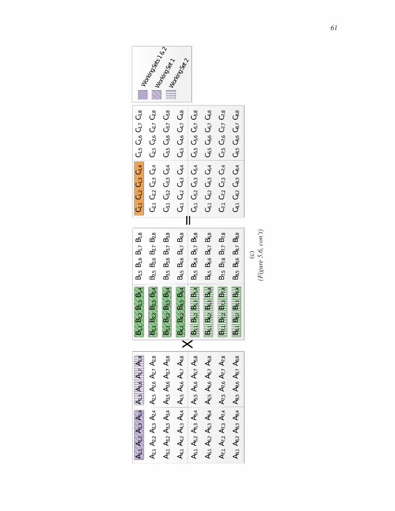
61
(c)
(Fig
ure
5.6,
con’
t)
62
cache residency and reuse; this is due to the fact that the dot products of a single row from that matrix
are computed against all columns of the right matrix, so it tends to reside in the cache for longer.
5.3.1.3 Blocked Matrix MultiplyStoring transposed matrices restricts the allowed operations performed on them—transposed ma-
trices can only participate as the “right matrix” in any multiplication. A common cache optimization
for the standard algorithm is instead to use blocking, in which submatrices are repeatedly multiplied
and accumulated in the final output. Rather than a single row of one matrix and a single value of one
column residing together in the cache at a time, blocking allows for the submatrices to occupy the
cache instead, occupying a middle ground between the standard and transposed algorithms, while
retaining the generality of standard matrix multiply.
Figures 5.1(c,d) show that the overall volume of cache misses is reduced, and more evenly
distributed between the matrices. As the submatrix lines are brought into cache, they remain there
relatively longer and get better data reuse than in the naive case.
5.3.2 Sorting AlgorithmsSorting algorithms are a natural choice for demonstrating reference trace visualization, as the
algorithms are usually straightforward and simple to implement and understand, and therefore have
simple yet important interactions with the cache. This section compares two well-known sorting
algorithms, uncovering their cache performance characteristics: bubble sort and merge sort. Bubble
sort is known for its slow O(n2) average-case running time, but it has good cache performance
characteristics. By contrast, merge sort has a better running time, its particular cache behavior
characteristics are demonstrated.
5.3.2.1 Bubble SortBubble sort is a well-known sorting algorithm with a very simple implementation, in which
repeated sweeps of the array to be sorted cause large items to be swapped to the end. After the
ith sweep, the ith largest element is sorted into place; therefore, the algorithm requires N sweeps
of steadily decreasing length in the worst case to sort the entire list. The visualization of the
memory behavior of this algorithm (Figure 5.7) shows an interesting characteristic—as the algorithm
nears completion, and the size of the remaining elements to sort begins to fit in the cache, cache
performance steadily improves. During the first sweep, all elements of the array are accessed in turn,
and the visualization shows every block of values entering and then exiting the cache. The L1 cache
temperature rises due to the high volume of swaps occuring there, while the L2 cools due to the
lack of available data reuse in that level (since each item is accessed at one time during each sweep).

63
Figure 5.7. Visualizing the cache behavior of bubble sort in Waxlamp. Bubble sort uses successive
sweeps to swap the remaining largest element to the correct location. Because the sweeps become
progressively shorter, the size of the working set continuously decreases until it fits first within L2,
and then within L1, leading to good cache behavior at the end of the algorithm.
However, because fewer and fewer elements are needed in each subsequent sweeps, eventually all
of the required data populates the L2—and then L1—cache, and no further evictions take place.
This is illustrated by the sustained flurry of activity between L1 and L2, and then later solely in L1,
indicated by frequent, localized streak lines and an increase in the observed cache temperatures. The
visualization clearly shows the increasing spatial locality inherent in the access patterns associated to
bubble sort.
Although bubble sort is famously slow in algorithmic complexity, it does in fact have—at least
during certain segments of its execution—desirable cache behavior. Though reasoning carefully
about bubble sort might lead to the insights about its execution presented here, Waxlamp makes the
insights immediately graspable—its value lies in its ability to quickly, decisively, and visually convey
those insights, which can then later be confirmed by reasoning about the program.
5.3.2.2 Merge SortMerge sort typifies the “efficient” sorting algorithms—it achieves the O(n logn) lower complexity
bound on comparison-based sorting algorithms. It is a divide-and-conquer algorithm that works by
dividing the list into two parts, applying the merge sort procedure recursively to each half, and then
reassembling a sorted list by sweeping each list, transferring the appropriate value to the result array.
Though the algorithm has good asymptotic complexity, it may be somewhat surprising to see that
its cache behavior is somewhat erratic. In the initial phase of the algorithm, the input is recursively
subdivided into a tree of lists of single elements (each of which is trivially already sorted, by
definition). In this phase, no memory transactions are performed on the elements, so its cache
performance is vacuously neutral. The second half of the merge sort algorithm builds the sorted

64
output by successively merging the single-element lists, then the two-element lists that result, etc.
This phase starts out with good cache performance, as the lists to be sorted are small and fit entirely
into L1 (Figure 5.8, right top), but as sorted elements begin to move farther and farther distances (as
they jump from their current position to the head of a progressively sorted subarray), spatial locality
degrades. This can be seen in the spilling over of the working set into L2 (Figure 5.8 right middle),
and then into main memory, with increasingly frequent bursts of cache misses as the merge phase
progresses (Figure 5.8 right bottom). At the midway point, the process begins again for the second
half of single-element lists, and the cache behavior recurs once more.
5.3.3 Material Point MethodThe material point method (MPM) [4] is a particle-based mechanical engineering simulation
method in which objects are discretized into collections of points, which undergo loads according to
certain rules. This section demonstrates a running MPM program, highlighting some of its cache
behaviors—a real-world example running in Waxlamp.
Figure 5.4 shows an MPM timestep at various points. Figure 5.4 left shows an early phase of the
timestep, in which the particle momenta (computed from their masses and velocities—the black and
purple data arrays, respectively) are interpolated to a background mesh via their positions (the green
data array).
Figure 5.4(middle) shows the particle stress update (the brown data array) taking place, with
input from the physical constitutive model (blue data array), using a sweeping access pattern that
will engage each particle in the system. As this action continues, the data seen to reside in L2, which
is no longer needed during this phase of the timestep, will slowly age and be pushed out by the
newer incoming data—the hallmark of a “streaming” style of access, which is embodied by the stress
update.
This example contains more data than the previous examples, and uses a larger cache with
quadruple the size of the earlier simulated caches. As Figure 5.4 right shows, Waxlamp is able to
scale up to larger sizes. Currently, the bottleneck lies on the data collection side, rather than the
visualization side.
5.4 Conclusions and Future WorkWaxlamp is a visualization system for memory reference traces, drawing inspiration from
organic visualization approaches, in reaching for the goal of illustrating the large-scale behavior
of memory access and caching during the run of a program. It uses cache simulation as a way to
drive performance analysis, and a carefully orchestrated set of visual qualities to convey important
information about a program’s runtime memory behavior.

65
Figure 5.8. Visualizing merge sort in Waxlamp. Left: A schematic view of how merge sort works.
In the top half, the sorting function is recursively called on each half of the input. This step simply
sets up a tree of computation that will accomplish the sorting, without any memory access. In the
lower half, atomic lists of a single element are combined successively by merging, resulting in
progressively larger, sorted sublists. This stage involves comparisons and movement of elements to a
temporary working store, before they are copied back to the input array. Each depicted merging phase
matches with a snapshot of Waxlamp on the right. Right: Visualization of the memory behavior
of the merge phase. This has roughly the opposite cache behavior as bubble sort—it begins its
memory transactions with small lists that fit entirely in the cache, forming progressively larger lists
that eventually overspill the cache levels, leading to poorer cache characteristics near the end of the
algorithm.

66
10 3 8 4 2 12 5 9
2 3 4 5 8 9 10 12
Split
Pha
se(n
o m
emor
y ac
tivity
)M
erge
Pha
se
10 3 8 4 2 12 5 9
8 4 2 12 5 910 3
10 3 8 4 2 12 5 9
4 8 2 12 5 93 10
3 4 8 10 2 5 9 12
67
Although Waxlamp’s design decisions work well to convey information, there is still possible
exploration of the visual channels discussed in this chapter. For instance, the low-frequency motion
chanel is largely unused in the current approach—mainly because it avoids clutter in the visualization—
but it may be the case that other effects in various visual channels are in fact useful. Prototypes for
several such effects, along with a well-designed user study, could help to evaluate such designed
objectively.
There is also no reason to restrict these techniques to just the memory subsystem. A crucial part of
Waxlamp rested in designing a meaningful static structure against which to overlay the dynamically
changing data glyphs. Such designs are possible for many different kinds of system architectures,
and that with the right kinds of data sources, the approach could be adapted to diverse computing
platforms. Aside from providing richer visual metaphors than MTV, Waxlamp is also abstract in this
way: it is an approach designed from the start to be adaptable to many different settings.
This chapter and the last have discussed to approaches to visualizing the contents of memory
reference traces, each with its own focus and visual setup, each delivering its own classes of insights.
The next chapter shifts the approach to examining reference traces themselves, electing to focus on
their structure, beyond the simple linear temporal flow assumed so far.
CHAPTER 6
COMPUTING AND VISUALIZING THE
TOPOLOGICAL STRUCTURE OF
MEMORY REFERENCE
TRACES
This chapter explores the topological structure of reference traces, attempting to go beyond the
obvious, temporally linear structure to find a correspondence with the underlying program behavior,
which itself is not always simply linear. Exposing the topological structure of reference traces brings
certain insights in and of itself, and may also serve to enhance visualization approaches such as MTV
and Waxlamp.
6.1 IntroductionA reference trace is fundamentally a time-varying signal expressing a program’s memory behavior,
event by event. As such, it has a trivially linear structure—it is simply a list of memory references.
However, an application generally has nonlinear programming constructs such as branches and loops,
which are evident in its source code. It is important to understand the dynamic memory behavior of a
program with respect to its static source code. In particular, a program exhibits spatial and temporal
locality, the tendency to reference nearby memory locations in relatively quick succession. Many
programs exhibit recurrent memory access patterns, which may or may not be directly reflected
through their programming constructs. For instance, a loop may execute several times, each time
accessing memory locations in similar patterns, therefore inducing a circular memory access pattern.
Conversely, two different stretches of the source code from two different functions may share similar
memory access patterns, if they both perform similar sets of reads and writes upon the memory.
Detecting and visualizing memory access patterns can lead to a better understanding of the
program behavior, as well as insights into its performance characteristics. This goal is accomplished
by encoding a nonlinear high dimensional structure over the memory reference trace, specifically re-
vealing its inherent circular behavior through topological analysis, while providing a correspondence

69
between the runtime memory behavior and the source code.
Topological analysis reveals complex, multiscale features in reference traces that would be
difficult to find using simple pattern matching approaches. The application of topological methods to
the seemingly unrelated field of software visualization is unexpected: in fact, such a nonstandard way
to compute and visualize the runtime behavioral structure of software can deliver surprising insight,
and therefore constitutes a valuable and novel contribution in itself. As this chapter demonstrates,
reference traces have a certain topological quality that can be extracted and used to compute
interesting structures which actually correspond to well-known programming structures. In other
words, topological methods can expose programming structures hidden in a reference trace, and for
this reason, the use of the heavy machinery of topology is justified.
This chapter describes an approach to study certain aspects of the temporal behavior of memory
reference traces through topological analysis and visualization. A skeleton of the approach is as
follows:
1. Sequences of consecutive memory accesses within the raw memory reference trace are recast
as points in a high-dimensional space, therefore creating a point cloud abstraction of the
temporal information encoded within the linear trace.
2. The point cloud is equipped with an architecturally meaningful metric, which reflects the simi-
larity between two sequences of memory accesses, thus capturing the notion of spatiotemporal
locality.
3. Automatic topological analysis on the point cloud detects circular structures which represent
the recurrent, cyclical memory behaviors.
4. Topological persistence guides the selection of meaningful circular structures: those with high
persistence likely represent significant features within the runtime behavior of a program.
5. A visualization approach connects the nonlinear runtime memory behaviors with program
source code, providing insights to potential performance optimizations.
In contrast to visualization solutions like CVT [93], cache behavior maps [99], YACO [72],
MTV (Chapter 4), and Waxlamp (Chapter 5), which provide various ways to visualize actual
moment-to-moment program memory behavior (see Chapter 3 for a deeper discussion), topological
analysis strives to compute a more global quality of the trace: higher-order structures that may extend
through time, forming cycles that may be executed multipile times. In that sense, this work is in
the same camp as reference affinity [100], which computes a different nonlinear structure over a
reference trace. de Silva et al. [23] and Wang et al. [95] present approaches to finding topological
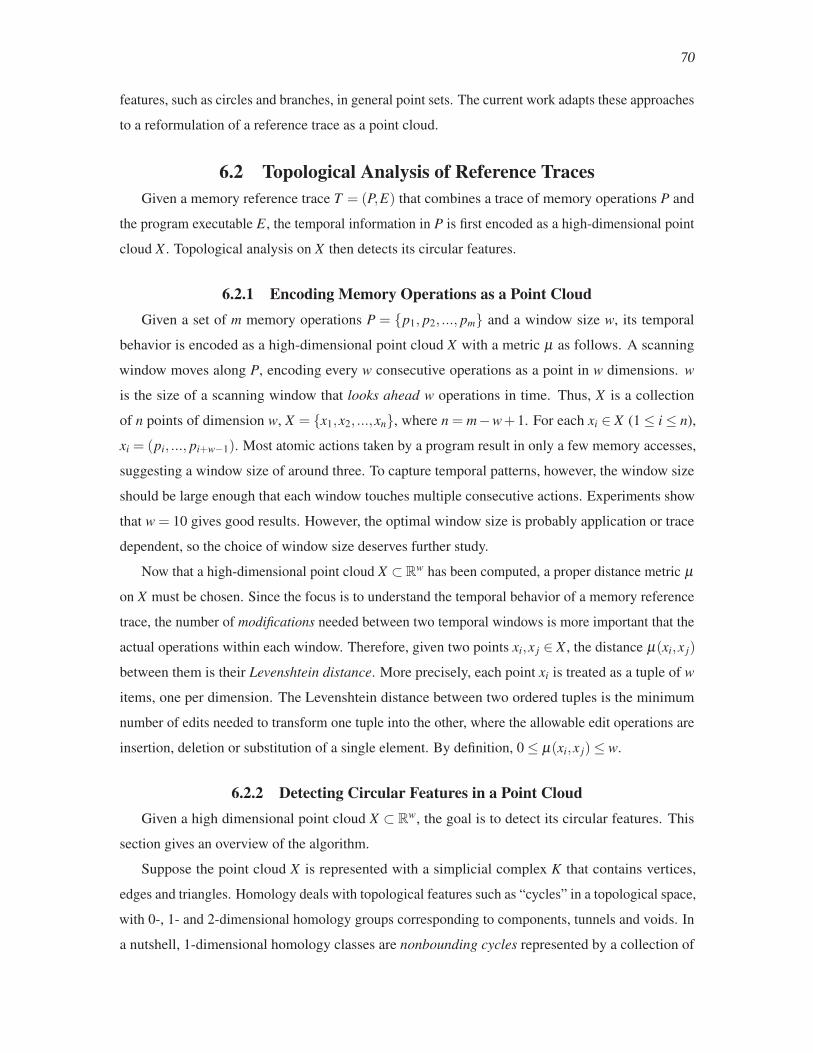
70
features, such as circles and branches, in general point sets. The current work adapts these approaches
to a reformulation of a reference trace as a point cloud.
6.2 Topological Analysis of Reference TracesGiven a memory reference trace T = (P,E) that combines a trace of memory operations P and
the program executable E, the temporal information in P is first encoded as a high-dimensional point
cloud X . Topological analysis on X then detects its circular features.
6.2.1 Encoding Memory Operations as a Point CloudGiven a set of m memory operations P = {p1, p2, ..., pm} and a window size w, its temporal
behavior is encoded as a high-dimensional point cloud X with a metric μ as follows. A scanning
window moves along P, encoding every w consecutive operations as a point in w dimensions. w
is the size of a scanning window that looks ahead w operations in time. Thus, X is a collection
of n points of dimension w, X = {x1,x2, ...,xn}, where n = m−w+1. For each xi ∈ X (1 ≤ i ≤ n),
xi = (pi, ..., pi+w−1). Most atomic actions taken by a program result in only a few memory accesses,
suggesting a window size of around three. To capture temporal patterns, however, the window size
should be large enough that each window touches multiple consecutive actions. Experiments show
that w = 10 gives good results. However, the optimal window size is probably application or trace
dependent, so the choice of window size deserves further study.
Now that a high-dimensional point cloud X ⊂ Rw has been computed, a proper distance metric μ
on X must be chosen. Since the focus is to understand the temporal behavior of a memory reference
trace, the number of modifications needed between two temporal windows is more important that the
actual operations within each window. Therefore, given two points xi,x j ∈ X , the distance μ(xi,x j)
between them is their Levenshtein distance. More precisely, each point xi is treated as a tuple of w
items, one per dimension. The Levenshtein distance between two ordered tuples is the minimum
number of edits needed to transform one tuple into the other, where the allowable edit operations are
insertion, deletion or substitution of a single element. By definition, 0 ≤ μ(xi,x j)≤ w.
6.2.2 Detecting Circular Features in a Point CloudGiven a high dimensional point cloud X ⊂ R
w, the goal is to detect its circular features. This
section gives an overview of the algorithm.
Suppose the point cloud X is represented with a simplicial complex K that contains vertices,
edges and triangles. Homology deals with topological features such as “cycles” in a topological space,
with 0-, 1- and 2-dimensional homology groups corresponding to components, tunnels and voids. In
a nutshell, 1-dimensional homology classes are nonbounding cycles represented by a collection of

71
edges in K. Dual to homology groups, 1-dimensional cohomology classes are nonbounding cocycles,
which are functions that map a collection of edges in K to integers.
The algorithm relies on the following principle from homotopy theory, which shows that in
an algebraic way, 1-dimensional cohomology represents circular structures in data. Let [X ,S1]
be the set of equivalence classes of continuous maps from the space X to the unit circle S1. Let
H1(X ;Z) be the group of 1-dimensional cohomology classes with integer coefficients. For topological
spaces with the homotopy type of a cell complex, there is an isomorphism (i.e., identical structure),
H1(X ;Z)∼= [X ,S1] [40]. This relates cohomology with circular coordinates. It implies that if X has
nontrivial 1-dimensional cohomology class α ∈ H1(X ;Z), we can construct a continuous function
θ : X → S1 from α (see [23] for a formal proof).
Given a point cloud X ⊂ Rw, global circular coordinate functions θ : X → S
1 can be computed,
that give the values for each point x in X . The overall pipeline is as follows:
1. Represent the point cloud data X as a family of simplicial complexes.
2. Use the concept of persistent cohomology [23, 95] to detect a significant cohomology class in
K, and convert such a class into a circle-valued function θ : X → S1.
3. Encode each circular coordinate in θ with a color map transfer function to highlight the circular
structures.
A high-level description of each step in the above process follows. An intuitive example follows
this description (Figure 6.1).
6.2.2.1 Step 1: Data Points to Simplicial ComplexA point cloud X ⊂ R
w with a metric μ can be represented as a single simplicial complex, or
more usefully as a nested family of simplicial complexes [22]. This analysis uses the Vietoris-Rips
complex, Rips(X ,ε), where there is a p-simplex for every finite set of p+1 points in X with diameter
at most ε . Since only H1 is required, its 2-skeleton is used, that is, the vertices, edges and triangles.
For ε0 ≤ ε1 ≤ ... ≤ εn, a nested family of simplicial complexes K : K(ε0) ⊆ ... ⊆ K(εn) results,
where K(εi) = Rips(X ,εi).
6.2.2.2 Step 2: Simplicial Complex to Circular CoordinateFunction
The nested family K of simplicial complexes represents the structure at different parameter
values ε , which encodes notion of spatial scale for learning the structure through the concept of
persistence. Persistence studies the evolution of vectors in a sequence of vector spaces [11]. One
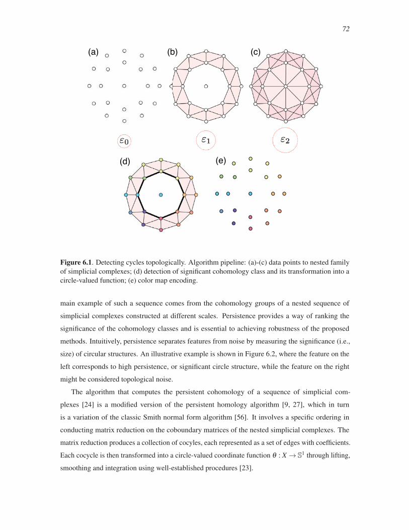
72
(a) (b) (c)
(e)(d)
Figure 6.1. Detecting cycles topologically. Algorithm pipeline: (a)-(c) data points to nested family
of simplicial complexes; (d) detection of significant cohomology class and its transformation into a
circle-valued function; (e) color map encoding.
main example of such a sequence comes from the cohomology groups of a nested sequence of
simplicial complexes constructed at different scales. Persistence provides a way of ranking the
significance of the cohomology classes and is essential to achieving robustness of the proposed
methods. Intuitively, persistence separates features from noise by measuring the significance (i.e.,
size) of circular structures. An illustrative example is shown in Figure 6.2, where the feature on the
left corresponds to high persistence, or significant circle structure, while the feature on the right
might be considered topological noise.
The algorithm that computes the persistent cohomology of a sequence of simplicial com-
plexes [24] is a modified version of the persistent homology algorithm [9, 27], which in turn
is a variation of the classic Smith normal form algorithm [56]. It involves a specific ordering in
conducting matrix reduction on the coboundary matrices of the nested simplicial complexes. The
matrix reduction produces a collection of cocyles, each represented as a set of edges with coefficients.
Each cocycle is then transformed into a circle-valued coordinate function θ : X → S1 through lifting,
smoothing and integration using well-established procedures [23].
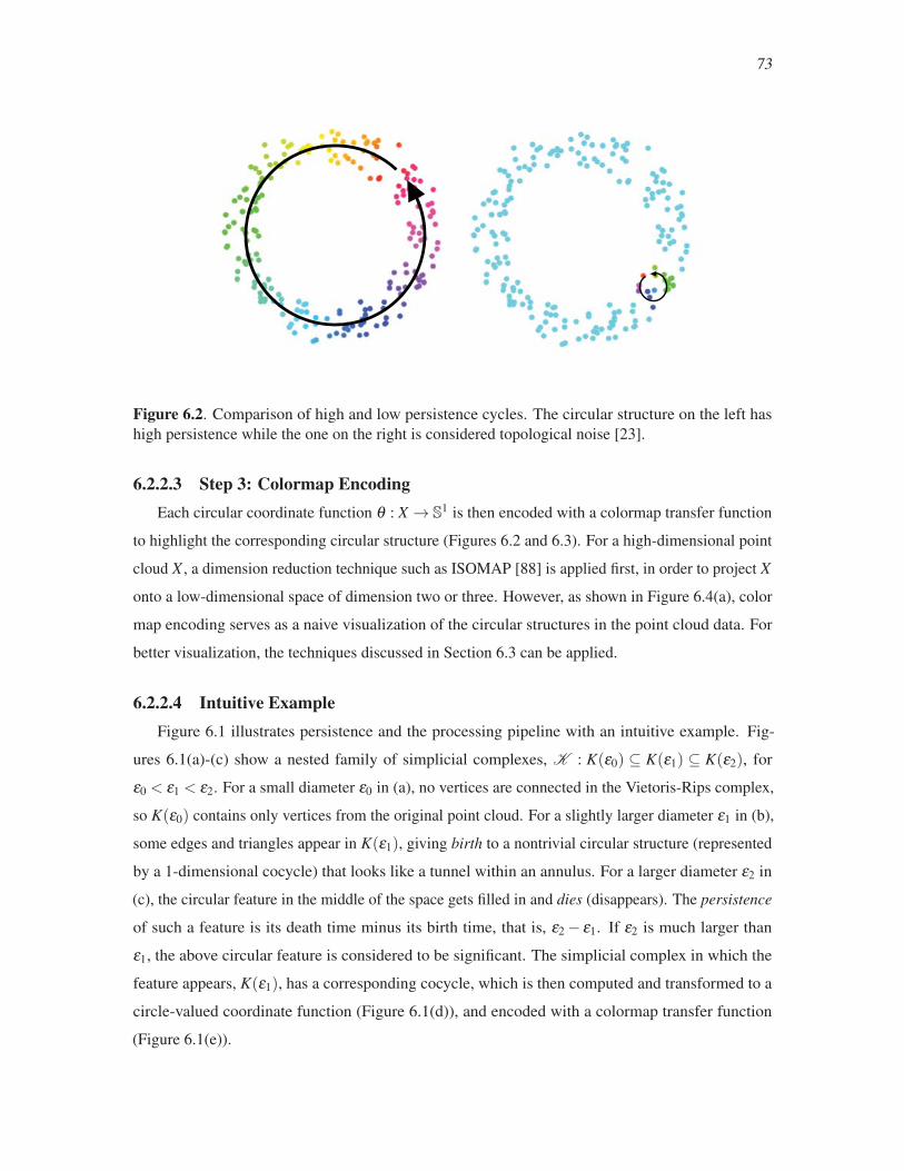
73
Figure 6.2. Comparison of high and low persistence cycles. The circular structure on the left has
high persistence while the one on the right is considered topological noise [23].
6.2.2.3 Step 3: Colormap EncodingEach circular coordinate function θ : X → S
1 is then encoded with a colormap transfer function
to highlight the corresponding circular structure (Figures 6.2 and 6.3). For a high-dimensional point
cloud X , a dimension reduction technique such as ISOMAP [88] is applied first, in order to project X
onto a low-dimensional space of dimension two or three. However, as shown in Figure 6.4(a), color
map encoding serves as a naive visualization of the circular structures in the point cloud data. For
better visualization, the techniques discussed in Section 6.3 can be applied.
6.2.2.4 Intuitive ExampleFigure 6.1 illustrates persistence and the processing pipeline with an intuitive example. Fig-
ures 6.1(a)-(c) show a nested family of simplicial complexes, K : K(ε0) ⊆ K(ε1) ⊆ K(ε2), for
ε0 < ε1 < ε2. For a small diameter ε0 in (a), no vertices are connected in the Vietoris-Rips complex,
so K(ε0) contains only vertices from the original point cloud. For a slightly larger diameter ε1 in (b),
some edges and triangles appear in K(ε1), giving birth to a nontrivial circular structure (represented
by a 1-dimensional cocycle) that looks like a tunnel within an annulus. For a larger diameter ε2 in
(c), the circular feature in the middle of the space gets filled in and dies (disappears). The persistence
of such a feature is its death time minus its birth time, that is, ε2 − ε1. If ε2 is much larger than
ε1, the above circular feature is considered to be significant. The simplicial complex in which the
feature appears, K(ε1), has a corresponding cocycle, which is then computed and transformed to a
circle-valued coordinate function (Figure 6.1(d)), and encoded with a colormap transfer function
(Figure 6.1(e)).

74
Figure 6.3. Detecting cycles in a genus-4 surface. Left: a point cloud X is sampled from a genus-4
surface. Right: four circle-valued coordinate functions correspond to its significant circular structures,
visualized by colormap transfer functions.
6.2.2.5 Parameter Selection and LimitationsThe foregoing topological analysis requires only one parameter, ε . It is used in computing the
2-skeleton of the Vietoris-Rips complex. In particular, for ε = ∞, computing the 2-skeleton of the
Vietoris-Rips complex for n high-dimensional points results in O(n3) simplices, giving a worst-case
time complexity of O(n3). This is, however, rare in practice [102]. The persistence algorithm runs
in time O(v3), where v is the number of simplices [12]. However, this takes roughly linear time
in practice [7]. Usually ε is chosen with prior knowledge of the problem domain, to be just large
enough to detect the topology, decreasing the above bound to an expected linear or even constant
behavior.
6.3 Visualizing Cycles in Reference TracesAs stated, dimension reduction techniques can work well for simple circular structures. The
technique can fail however when the high-dimensional structure of the memory reference trace
becomes complicated. Figure 6.4(b) shows an example where dimension reduction produces a
visualization which is extremely difficult to interpret. What is needed instead is a visualization
approach that is more robust to complex structure.
6.3.1 Circular VisualizationAs an alternative, the circular parameterization θ of all points can be used to formulate a
visualization. The parameter θ is first conditioned by performing a scale and offset such that
θ ∈ [0 : 2π]. θ contains points which are cycle members, but may also contain nonmembers in the
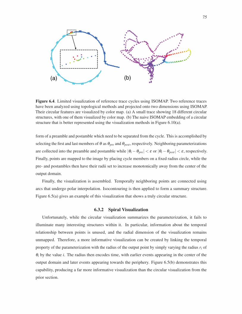
75
(a) (b)
Figure 6.4. Limited visualization of reference trace cycles using ISOMAP. Two reference traces
have been analyzed using topological methods and projected onto two dimensions using ISOMAP.
Their circular features are visualized by color map. (a) A small trace showing 18 different circular
structures, with one of them visualized by color map. (b) The naive ISOMAP embedding of a circular
structure that is better represented using the visualization methods in Figure 6.10(a).
form of a preamble and postamble which need to be separated from the cycle. This is accomplished by
selecting the first and last members of θ as θpre and θpost , respectively. Neighboring parameterizations
are collected into the preamble and postamble while |θi −θpre|< ε or |θi −θpost |< ε , respectively.
Finally, points are mapped to the image by placing cycle members on a fixed radius circle, while the
pre- and postambles then have their radii set to increase monotonically away from the center of the
output domain.
Finally, the visualization is assembled. Temporally neighboring points are connected using
arcs that undergo polar interpolation. Isocontouring is then applied to form a summary structure.
Figure 6.5(a) gives an example of this visualization that shows a truly circular structure.
6.3.2 Spiral VisualizationUnfortunately, while the circular visualization summarizes the parameterization, it fails to
illuminate many interesting structures within it. In particular, information about the temporal
relationship between points is unused, and the radial dimension of the visualization remains
unmapped. Therefore, a more informative visualization can be created by linking the temporal
property of the parameterization with the radius of the output point by simply varying the radius ri of
θi by the value i. The radius then encodes time, with earlier events appearing in the center of the
output domain and later events appearing towards the periphery. Figure 6.5(b) demonstrates this
capability, producing a far more informative visualization than the circular visualization from the
prior section.

76
(a)
(b)
(c)
(d)
Figu
re6.
5.V
isual
izat
ion
opti
ons
for
refe
rence
trac
ecy
cle
dat
a.(a
)T
he
par
amet
eriz
atio
nis
pla
ced
ina
circ
ula
rst
ruct
ure
.(b
)T
ime
isap
pli
edto
the
radiu
s.(c
-d)
The
dat
apoin
tsar
eco
rrel
ated
bac
kto
sourc
eco
de
usi
ng
aco
lor
map
.
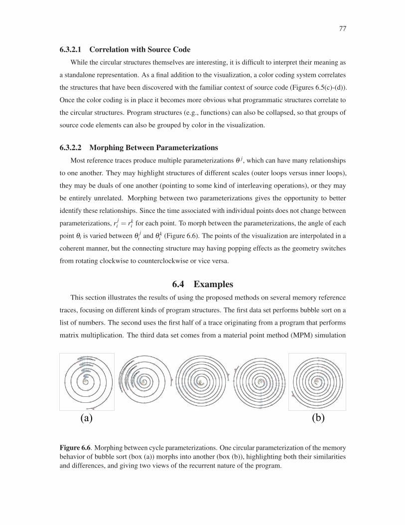
77
6.3.2.1 Correlation with Source CodeWhile the circular structures themselves are interesting, it is difficult to interpret their meaning as
a standalone representation. As a final addition to the visualization, a color coding system correlates
the structures that have been discovered with the familiar context of source code (Figures 6.5(c)-(d)).
Once the color coding is in place it becomes more obvious what programmatic structures correlate to
the circular structures. Program structures (e.g., functions) can also be collapsed, so that groups of
source code elements can also be grouped by color in the visualization.
6.3.2.2 Morphing Between ParameterizationsMost reference traces produce multiple parameterizations θ j, which can have many relationships
to one another. They may highlight structures of different scales (outer loops versus inner loops),
they may be duals of one another (pointing to some kind of interleaving operations), or they may
be entirely unrelated. Morphing between two parameterizations gives the opportunity to better
identify these relationships. Since the time associated with individual points does not change between
parameterizations, r ji = rk
i for each point. To morph between the parameterizations, the angle of each
point θi is varied between θ ji and θ k
i (Figure 6.6). The points of the visualization are interpolated in a
coherent manner, but the connecting structure may having popping effects as the geometry switches
from rotating clockwise to counterclockwise or vice versa.
6.4 ExamplesThis section illustrates the results of using the proposed methods on several memory reference
traces, focusing on different kinds of program structures. The first data set performs bubble sort on a
list of numbers. The second uses the first half of a trace originating from a program that performs
matrix multiplication. The third data set comes from a material point method (MPM) simulation
��� ���
Figure 6.6. Morphing between cycle parameterizations. One circular parameterization of the memory
behavior of bubble sort (box (a)) morphs into another (box (b)), highlighting both their similarities
and differences, and giving two views of the recurrent nature of the program.

78
code, which involves particles moving on a grid.
Table 6.1 enumerates the details of the data used for these experiments. The processing of data
through the pipeline takes on the order of a few minutes, while the most time consuming component
is collecting the memory trace, which takes on the order of a few seconds to a few minutes for these
examples. Computing the parameterizations takes on the order of seconds, and the visualization
renders at highly interactive rates. Topological persistence guides our selection of meaningful circular
structures. In general, all circular features selected have high persistence rankings, indicating their
significance.
The following sections demonstrate that the method offers insights into various nonlinear memory
behavior structures by connecting the source code with topological analysis and visualization.
6.4.1 Analyzing Loop ContentsThe bubble sort dataset demonstrates loop-based recurrent behavior. Bubble sort works by
repeatedly sweeping through the list to be sorted, comparing each pair of adjacent items and
swapping them if they are in the wrong order. These sweeps become progressively shorter as items
are sorted into place. For example, as shown in Figure 6.7(left column), sorting through a list of five
ascending-ordered numbers results in four standalone comparisons, while sorting through a list of
five descending-ordered numbers performs 10 comparisons followed by swaps. Sorting the given list
Table 6.1. Details of the data used in topological analysis experiments.
Data Set OriginalTrace Size
RecordsUsed
SampleInterval
PersistenceRank
Parameterizations
Bubble sort using vector (Fig. 6.7)Sorted 141K 680 1 (a) 1 (b) 1 14
Reverse 141K 1275 1 (c) 2 (d) 1 6
Shuffled 141K 1115 1 (e) 2 (f) 1 2
Bubble sort using array (Fig. 6.7)Sorted 141K 460 1 (g) 1 6
Reverse 141K 690 1 (h) 1 3
Matrix multiply (Fig. 6.8)Standard 173K 1000 1 (a) 3 (b) 2 (c) 1 4
Blocked 92K 1000 1 (d) 2 (e) 1 (f) 1 4
Material point method, 5 particles (Fig. 6.10)Interpolation 1.0M 2000 1 (a) 1 (b) 1 9
Material point method, 60 particles (Fig. 6.11)Fig. 6.11(a) 2.8M 1000 1 (a) 2 2
Fig. 6.11(b-c) 2.8M 10000 10 (b) 3 (c) 1 5
79
of randomly shuffled numbers results in six comparisons followed by swaps, and four standalone
comparisons.
Figure 6.7 shows various recurrent runtime structures captured by the proposed method, with each
image highlighting some specific features of the algorithm computation. Figures 6.7(a) and 6.7(b)
represent memory structures within sorting five ascending-ordered numbers. Figure 6.7(a) shows
four circular structures corresponding to the comparison operation occurring in the if statement (line
5). The circle itself represents one of the two C++ Standard Template Library (STL) vector lookups,
while the zig-zag secondary feature corresponds to the other. It serves to distinguish the two instances
of vector lookups while keeping the recurrent nature of comparisons in view. On the other hand,
Figure 6.7(b) shows each lookup on its own circle. There are two vector lookups per comparison,
with four independent comparisons leading to a total of eight circles. This image shows that the two
vector lookups occurring per comparison have almost identical memory signatures, which is not
directly evident in the source code. To better understand the correlations between these two circular
features, a morphing between them (Figure 6.6) showcases the expansions of secondary features
from Figure 6.7(a) to (b).
Figure 6.7(c) and 6.7(d) show a bubble sort proceeding on a descending-ordered list. In (c),
the outer loop (line 2) forms the four circles, while the 10 comparisons followed by swaps appear
as tooth-like features within each repetition, showcasing the properties of the input data, and the
corresponding computational structure of the algorithm. By contrast, (d) indicates the recurrent
structure of the inner loop (line 4). Each of the 10 bundled circular structures contains three circular
substructures, which reflect two vector lookups in the comparison (line 5) and one swap (line
6). Here, the appearance of properly spaced bundles serves to separate the important recurring
features. Figure 6.7(e) represents the sorting of five random-ordered numbers. The circular structures
correspond to the six comparisons followed by swaps, while the blue tooth-like features indicate
the four standalone comparisons that are not followed by swaps. The analysis is able to pick up on
this feature, encoded in the neighborhood information in the point cloud, which turns out to have
significance in this program. By contrast, Figure 6.7(f) is the dual of Figure 6.7(e), showing the
nonswapping comparisons as cycles, and the swapping comparisons as tooth-like features.
For comparison, Figure 6.7(g-h) shows a version of the bubble sort program that uses bare
arrays rather than STL vectors. Note that Figures 6.7(g) and (h) have similar memory signatures
as Figures 6.7(b) and (c), respectively, but with fewer memory accesses. Although the volume of
memory access changes due to modifications of data structures, the characteristics of the memory
behavior stay the same.
80
Figure 6.7. Visualizing reference trace cycles in bubble sort. Various recurrent runtime structures
are visible within a bubble sort of five numbers (a–b) in ascending order, (d–e) in descending order,
and (g–h) in random order. (c,f) Versions of (b) and (e) in which a bare array has been used in place
of STL vectors, eliminating many overhead memory accesses associated with the STL.
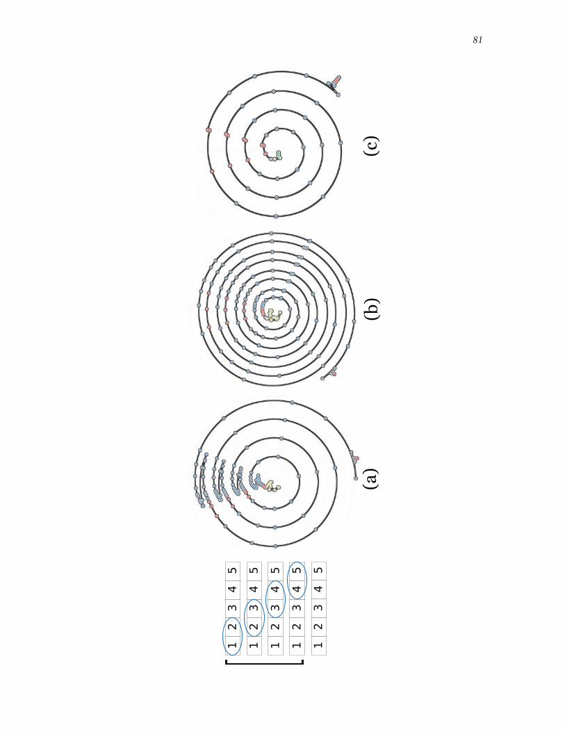
81
��
��
���
��
��
��
��
��
��
� ��
��
�
���
���
���

82
��
��
��
��
��
��
��
��
��
��
��
��
��
��
��
��
��
���
��
��
��
��
��
��
�
��
��
�
���
���
���
(Fig
ure
6.7,
con’
t)
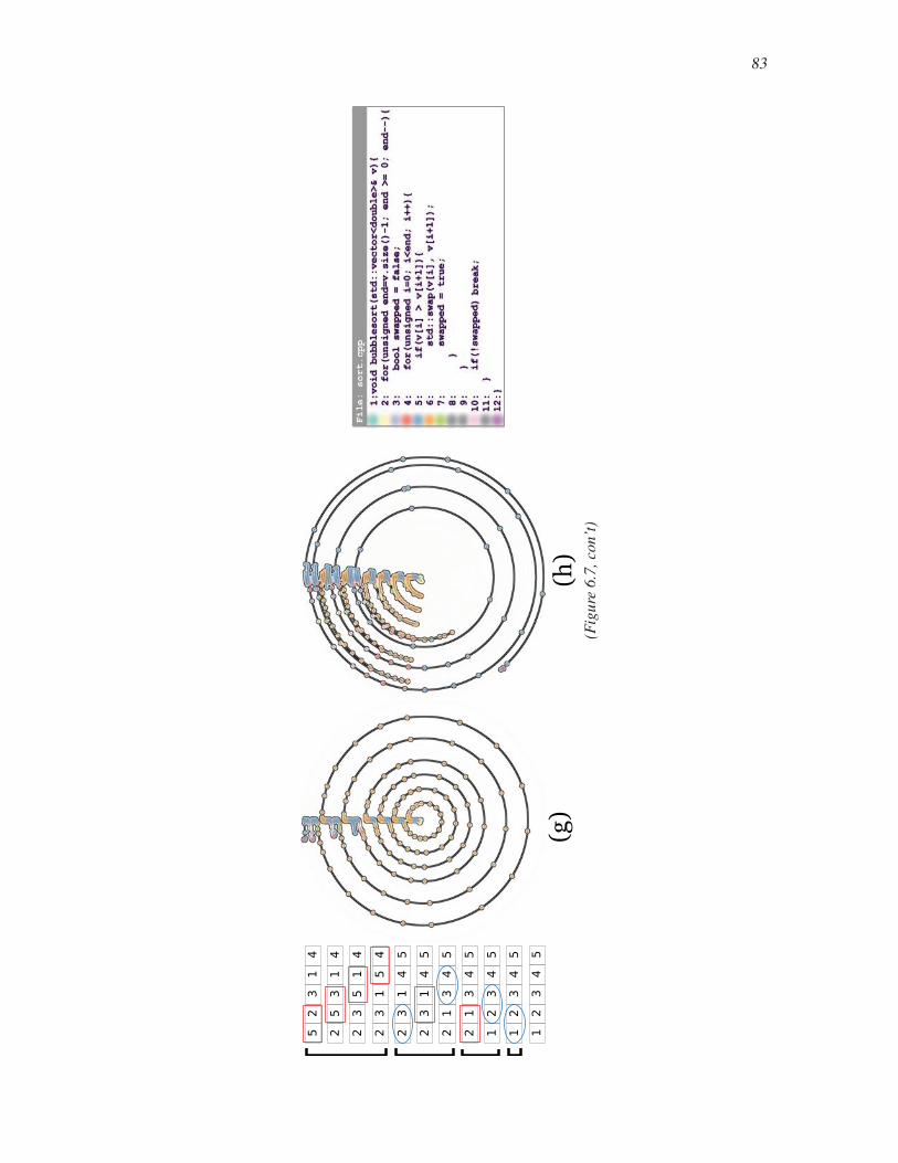
83
��
��
��
��
��
��
��
��
��
��
��
��
��
��
��
��
��
���
��
��
��
��
��
��
�
��
��
�
���
���
(Fig
ure
6.7,
con’
t)
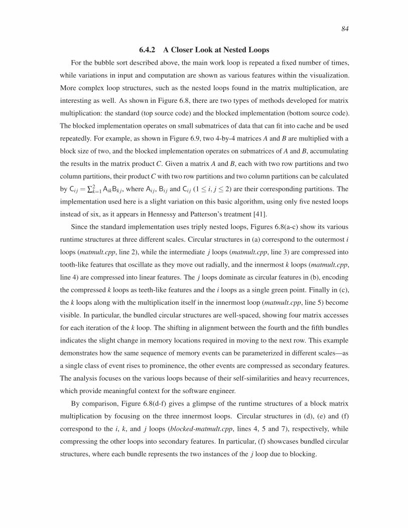
84
6.4.2 A Closer Look at Nested LoopsFor the bubble sort described above, the main work loop is repeated a fixed number of times,
while variations in input and computation are shown as various features within the visualization.
More complex loop structures, such as the nested loops found in the matrix multiplication, are
interesting as well. As shown in Figure 6.8, there are two types of methods developed for matrix
multiplication: the standard (top source code) and the blocked implementation (bottom source code).
The blocked implementation operates on small submatrices of data that can fit into cache and be used
repeatedly. For example, as shown in Figure 6.9, two 4-by-4 matrices A and B are multiplied with a
block size of two, and the blocked implementation operates on submatrices of A and B, accumulating
the results in the matrix product C. Given a matrix A and B, each with two row partitions and two
column partitions, their product C with two row partitions and two column partitions can be calculated
by Ci j = ∑2k=1AikBk j, where Ai j, Bi j and Ci j (1 ≤ i, j ≤ 2) are their corresponding partitions. The
implementation used here is a slight variation on this basic algorithm, using only five nested loops
instead of six, as it appears in Hennessy and Patterson’s treatment [41].
Since the standard implementation uses triply nested loops, Figures 6.8(a-c) show its various
runtime structures at three different scales. Circular structures in (a) correspond to the outermost i
loops (matmult.cpp, line 2), while the intermediate j loops (matmult.cpp, line 3) are compressed into
tooth-like features that oscillate as they move out radially, and the innermost k loops (matmult.cpp,
line 4) are compressed into linear features. The j loops dominate as circular features in (b), encoding
the compressed k loops as teeth-like features and the i loops as a single green point. Finally in (c),
the k loops along with the multiplication itself in the innermost loop (matmult.cpp, line 5) become
visible. In particular, the bundled circular structures are well-spaced, showing four matrix accesses
for each iteration of the k loop. The shifting in alignment between the fourth and the fifth bundles
indicates the slight change in memory locations required in moving to the next row. This example
demonstrates how the same sequence of memory events can be parameterized in different scales—as
a single class of event rises to prominence, the other events are compressed as secondary features.
The analysis focuses on the various loops because of their self-similarities and heavy recurrences,
which provide meaningful context for the software engineer.
By comparison, Figure 6.8(d-f) gives a glimpse of the runtime structures of a block matrix
multiplication by focusing on the three innermost loops. Circular structures in (d), (e) and (f)
correspond to the i, k, and j loops (blocked-matmult.cpp, lines 4, 5 and 7), respectively, while
compressing the other loops into secondary features. In particular, (f) showcases bundled circular
structures, where each bundle represents the two instances of the j loop due to blocking.

85
(a)
(b)
(c)
(d)
(e)
(f)
Figure 6.8. Recurrent runtime structures in matrix multiplication algorithms. (a-c) Standard matrix
multiplication. (d-f) Blocked matrix multiplication. Top: source code for standard implementation.
Bottom: source code for blocked implementation.
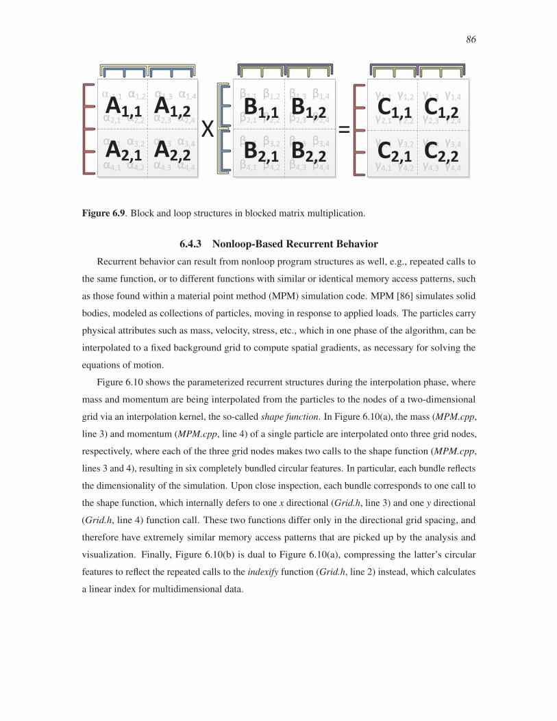
86
X =β1,1 β1,2 β1,3 β1,4
β2,1 β2,2 β2,3 β2,4
β3,1 β3,2 β3,3 β3,4
β4,1 β4,2 β4,3 β4,4
γ1,1 γ1,2 γ1,3 γ1,4
γ2,1 γ2,2 γ2,3 γ2,4
γ3,1 γ3,2 γ3,3 γ3,4
γ4,1 γ4,2 γ4,3 γ4,4
α 1,1 α1,2 α1,3 α1,4
α2,1 α2,2 α2,3 α2,4
α3,1 α3,2 α3,3 α3,4
α4,1 α4,2 α4,3 α4,4
A1,1 A1,2
A2,1 A2,2
B1,1 B1,2
B2,1 B2,2
C1,1 C1,2
C2,1 C2,2
Figure 6.9. Block and loop structures in blocked matrix multiplication.
6.4.3 Nonloop-Based Recurrent BehaviorRecurrent behavior can result from nonloop program structures as well, e.g., repeated calls to
the same function, or to different functions with similar or identical memory access patterns, such
as those found within a material point method (MPM) simulation code. MPM [86] simulates solid
bodies, modeled as collections of particles, moving in response to applied loads. The particles carry
physical attributes such as mass, velocity, stress, etc., which in one phase of the algorithm, can be
interpolated to a fixed background grid to compute spatial gradients, as necessary for solving the
equations of motion.
Figure 6.10 shows the parameterized recurrent structures during the interpolation phase, where
mass and momentum are being interpolated from the particles to the nodes of a two-dimensional
grid via an interpolation kernel, the so-called shape function. In Figure 6.10(a), the mass (MPM.cpp,
line 3) and momentum (MPM.cpp, line 4) of a single particle are interpolated onto three grid nodes,
respectively, where each of the three grid nodes makes two calls to the shape function (MPM.cpp,
lines 3 and 4), resulting in six completely bundled circular features. In particular, each bundle reflects
the dimensionality of the simulation. Upon close inspection, each bundle corresponds to one call to
the shape function, which internally defers to one x directional (Grid.h, line 3) and one y directional
(Grid.h, line 4) function call. These two functions differ only in the directional grid spacing, and
therefore have extremely similar memory access patterns that are picked up by the analysis and
visualization. Finally, Figure 6.10(b) is dual to Figure 6.10(a), compressing the latter’s circular
features to reflect the repeated calls to the indexify function (Grid.h, line 2) instead, which calculates
a linear index for multidimensional data.
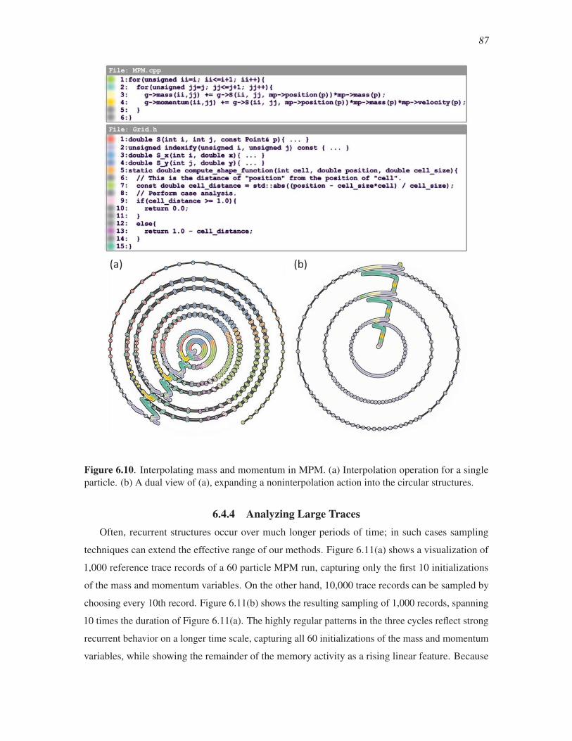
87
(a) (b)
Figure 6.10. Interpolating mass and momentum in MPM. (a) Interpolation operation for a single
particle. (b) A dual view of (a), expanding a noninterpolation action into the circular structures.
6.4.4 Analyzing Large TracesOften, recurrent structures occur over much longer periods of time; in such cases sampling
techniques can extend the effective range of our methods. Figure 6.11(a) shows a visualization of
1,000 reference trace records of a 60 particle MPM run, capturing only the first 10 initializations
of the mass and momentum variables. On the other hand, 10,000 trace records can be sampled by
choosing every 10th record. Figure 6.11(b) shows the resulting sampling of 1,000 records, spanning
10 times the duration of Figure 6.11(a). The highly regular patterns in the three cycles reflect strong
recurrent behavior on a longer time scale, capturing all 60 initializations of the mass and momentum
variables, while showing the remainder of the memory activity as a rising linear feature. Because
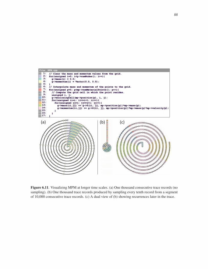
88
(a) (b) (c)
Figure 6.11. Visualizing MPM at longer time scales. (a) One thousand consecutive trace records (no
sampling). (b) One thousand trace records produced by sampling every tenth record from a segment
of 10,000 consecutive trace records. (c) A dual view of (b) showing recurrences later in the trace.

89
of this “time compression” effect, each of these cycles no longer correlates directly to a specific
line of source code, but rather expresses general program structures. Figure 6.11(c) is the dual of
(b), showing the initialization phase as a linear structure, and expanding the remainder of the trace,
interpolation of the mass and momentum to the background grid, as time-sampled cycles.
By increasing the sampling interval, a much longer trace can be displayed while keeping the
ability to distinguish different parts of the program. Sampling the trace allows the analysis to find
large-scale structures, providing a picture of the entire run of a program, rather than details of
individual functions, loops, or lines of code. As such, sampling can be used to manage level-of-detail
for reference traces.
6.4.5 Performance-Related BehaviorWhen the visualization reveals recurrent runtime behavior that reflects the repetitive nature
of a portion of the program, it can suggest potential performance optimizations. For example,
in Figure 6.10(a) the two bundled circles represent nearly identical function executions, differing
only in the value of a single parameter, suggesting that the two executions could coalesce into one,
sparing the duplication of several computations and memory accesses. This is similar to the idea
of loop fusion [47], in which loop bodies from independent loops may be combined to eliminate
loop overheads and gain possible caching benefits from increased data reference locality. Knowing
whether transformation would increase performance requires further study, and probably a host of
new tools such as execution models etc., but the focus of the current technique lies in highlighting
the possibility, which is much harder to see with existing techniques.
The approach also reveals the circular structures of program constructs usually hidden by
programming abstractions, such as helper functions, standard libraries, or operator overloading.
For example, as shown in Figure 6.7(d), in the bubble sort case study, using the STL vectors
involves many more memory accesses than the naive implementation. Programmers may not be
fully conscious of such complexities within the STL, due to its heavy use of abstraction, but this
visualization approach may suggest places where such extra memory references can be eliminated.
Though other techniques exist for simply counting memory accesses, the current approach highlights
the difference visually while pointing out the cyclical nature of both programs, thus adding value
over previous approaches.
6.4.6 Topological PersistenceThe use of topological persistence is a major strength of the approach. Once the parameter ε is
chosen, topological analysis proceeds automatically to detect circular structures. Once running, the
analysis does not require fine-tuning of parameters or user intervention. Then, topological persistence

90
guides the selection of meaningful circular structures. As the examples strongly suggest, those with
high persistence likely represent significant features within the runtime behavior of a program. As
displayed in Table 6.1, all significant circular features presented have highly ranked persistence.
Furthermore, there is a clear separation in persistence measures between interesting and trivial
circular features.
6.5 ConclusionsThis topological approach represents a general framework for exploring and discovering recurrent
behavioral patterns in memory reference traces. We first recast a list of reference trace records, a
staple of software memory analysis, as a high-dimensional point cloud. We then employ topological
analysis to detect its circular features. The novelty of the work lies in (a) the design of a proper
metric that allows the computation of meaningful circular structures, based on the nature of source
code and the program runtime behavior, and (b) the application of topological analysis of circular
features within the field of software visualization. Both loop-based and nonloop-based recurrent
structures can be captured by the analysis and visualization. While the former confirms the expected
structures of a program, the latter highlights less obvious features that are possible candidates for
performance optimization.
With this chapter on topological analysis, this dissertation concludes string of novel transfor-
mations on individual reference traces: MTV and Waxlamp give two different visual encodings of
the reference trace data, while t his chapter computes cyclical structures over the trace, providing a
visual mapping for displaying them. The next chapter takes a longer perspective, exploring the kinds
of insight that can be gained from examining multiple reference traces at the same time.
CHAPTER 7
VISUALIZING DIFFERENTIAL BEHAVIOR IN
MEMORY REFERENCE TRACES USING
CACHE SIMULATION ENSEMBLES
The preceding three chapters introduced several ideas for processing individual reference trace
in order to focus on their various particular qualities. By contrast, this chapter is concerned with
ensembles of reference traces, in order to derive insight from the differences in behavior among
several traces or simulations. Several case studies will be presented to demonstrate the usefulness of
this approach.
7.1 IntroductionBecause of the relative scarcity of high-performance computing resources, many computational
applications have program performance as a primary design goal. Hardware performance predic-
tion [48] and software analysis [66] can be used to help guide new hardware deployments and
software optimization efforts, but these approaches are generally approximate, because of the many
complex interactions among computer subsystems. These subsystems include data storage, network,
functional units, and memory, all dealing with many events occurring at once, such as incoming
messages, hardware interrupts, randomized process scheduling, and shifting computational loads.
Such conditions vary from machine to machine, operating system to operating system, execution to
execution, and even from moment to moment within a particular run, producing uncertainty in the
perception and measurement of program performance.
Throughout this dissertation, cache behavior and performance have been the primary objects of
study. However, measuring cache performance is complicated by the system performance uncertainty
mentioned above. Furthermore, variability in caches across multiple systems, as well as differences
between software implementation choices, leads to a kind of uncertainty or variation specific to
memory and cache performance.
This chapter presents approaches for analyzing the performance uncertainties induced by design
decisions in algorithms and memory caches, leading to insight about program performance and

92
possible software optimizations. Memory caches have many design features that affect performance,
which are usually outside the control of a software developer. Nevertheless, understanding how
software performance changes with cache design can yield insight about, for instance, the stability or
robustness of cache performance. Features within the developer’s control, such as choice of algorithm
or how to lay out data in memory, are another source of variation that can be analyzed with this
approach. Finally, changing resource allocation on the running system may cause varying amounts
of available cache for a particular program—the techniques allow for the analysis of this third source
of uncertainty. The insights thus gleaned can be used to make design choices for software that may
run on different kinds of machines, or they may affect the choice of algorithm used in a production
run on a particular machine.
Varying execution conditions, such as cache configuration parameters or algorithmic imple-
mentation details, results in several reference traces and simulated caches that, when combined,
yield a simulation ensemble of all the runs under study. When visualized, these ensembles can
yield insight about cache performance characteristics about both software and hardware, and the
relationship between the two. A specific visual technique, based on Waxlamp (Chapter 5), is also
presented for highlighting the differences between a pair of reference traces with respect to memory
distribution in a cache, enabling an investigation into just how the cache behavior changes under
some set of differences. Figure 7.1 shows examples of both approaches. The graphs on the right
represent three different ensembles that use caches of different L1, L2, and total size, plotting the
resulting performance of a reference trace, while the figures on the left show detailed differences in
the simulations for two of the caches.
Ensembles capture uncertainty by running the same computation over a number of different
conditions and coordinating the results into a single dataset. A common example is a set of weather
forecasting models, each run multiple times with different initial conditions [70, 76]. By seeing
where the ensemble members agree and disagree, it becomes easier to make accurate forecasts, and
more generally to derive insight about why a particular model might differ in its prediction [70].
Visualization of ensembles usually plots some combination of the ensemble members over a
model of the domain on which the data resides (e.g., a map of the earth for climate models). Spaghetti
plots show the ensemble members all plotted together, showing similarities and differences at a glance.
Glyphs can also be used to indicate the variation between the members without visual clutter [76].
The spatial or physical aspect can also be abstracted way, leaving just the raw data; statistical
measures such as mean and standard deviation can then be plotted in more traditional information
visualization views [70]. More generally, techniques for visualizing uncertainty—whether it results
from an ensemble or a separate source—include glyph-based approaches [69, 76], colormaps, and

93
Figure 7.1. Overview of visualization for cache simulation ensembles, showing a memory reference
trace for bubble sort being run through a variety of simulated caches differing in size. The top images
show “visual diffs” of a pair of cache simulations differing only in the size of the cache, shown at
different points in time, while the bottom images show graphs of the cache access times of simulation
ensembles including these two traces, and more. (a) Both simulations show equal performance,
always finding required data in the same level of the cache, even though the difference in size means
that the data may be found in different parts of the same cache levels. The associated graphs are
exactly equal in this regime. (b) One of the simulations can now fit all its data into the L2 level of the
cache. Darker lines show data for the two simulations coming from different levels of the cache (L2
and main memory), highlighting their differences. Note that the green and purple lines have begun to
disagree in the ensemble. (c) After some time, one simulation can fit into L1, while the other is still
in L2. The graph shows better performance for both compared to (a) and (b), while the visual diff
shows the precise differences between the accesses being performed in each simulation.
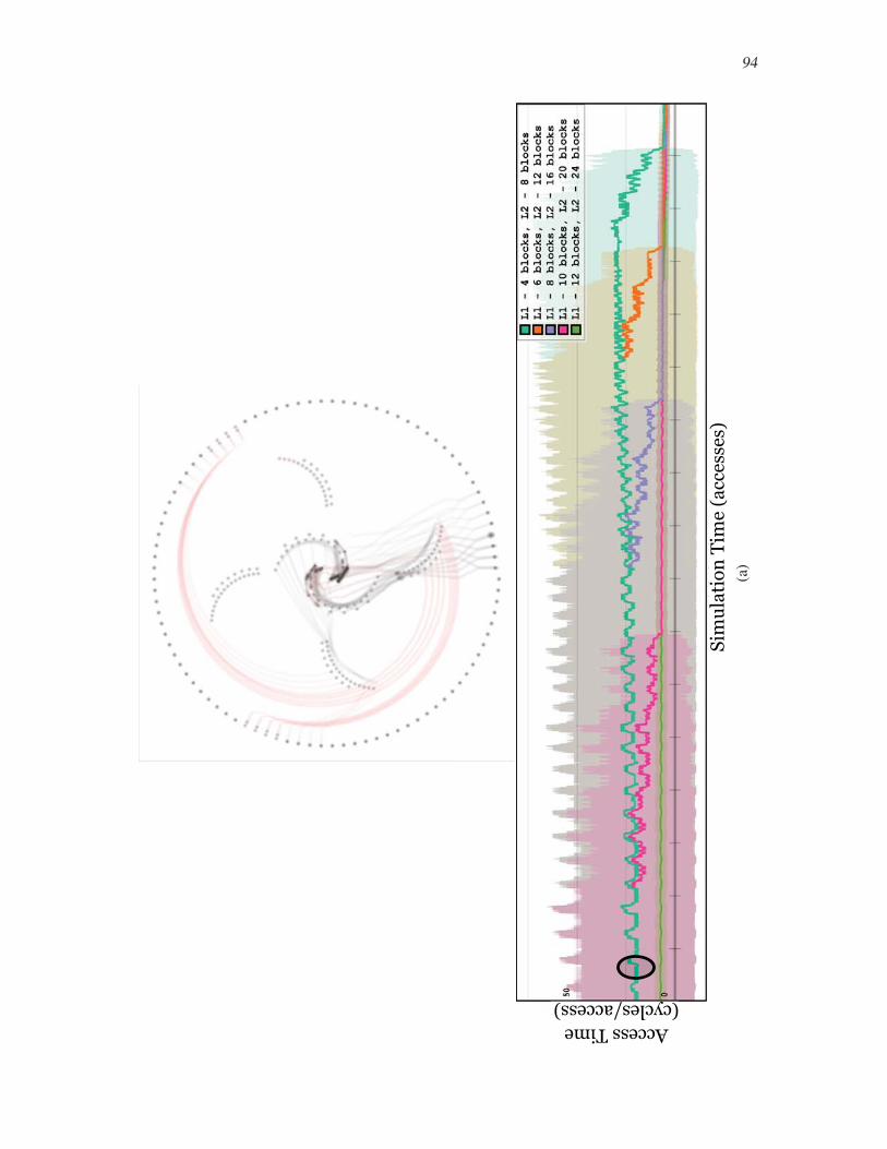
94
���������������� �������
�����������������������
(a)
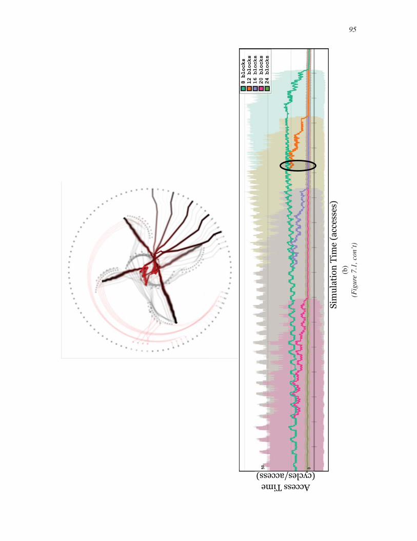
95
������������ ����� �� ��
��� ������ ����� ����� ���
(b)
(Fig
ure
7.1,
con’
t)

96
������������ ����� �� ��
��� ������ ����� ����� ���
(c)
(Fig
ure
7.1,
con’
t)

97
overlaying uncertainty data over the data to be visualized [65].
In this chapter, the model is an abstract representation of the levels of a cache, while the simulation
output encodes changes to the state of the cache. As such, concrete techniques such as the spaghetti
plot are not directly applicable, though the Waxlamp approach (Chapter 5) is adapted to create
“visual diffs” between members of a simulation ensemble. Furthermore, the nonspatial idea is used to
compute and plot statistics over various measures of the simulation results. These approaches can
begin to bring insight about program behavior from differences between cache simulation ensemble
members.
7.2 Cache Performance UncertaintyUncertainty in caching can occur in two major ways: first, the program being executed might
change from run to run (e.g., using different input data, data structures with different layouts, or
different algorithms to carry out the work); second, the cache configuration itself might change from
run to run. The first case encompasses end users running programs for their own purposes, as well
as software engineers seeking to improve their code—profilers and simple wall-clock timing are
often used to evaluate such changes in program elements. The second case is usually the purview of
computer architects designing a suitable cache architecture for a target computer system. However,
taking on the mindset of the architect and playing with different cache configurations can actually
produce insight about software. For instance, the concept of the working set is important when
considering the cache behavior of a given program, and it can be probed in cache ensembles by
varying the size of the simulated cache. Figure 7.2 summarizes the sources of cache performance
uncertainty.
Data Features�� Data Size�� Data Value�� Data Order
Software Features�� Algorithm�� Data Layout
Architectural Features�� Cache Latency�� Cache Size�� Cache Associativity�� Memory Architecture
Figure 7.2. Sources of variation in cache performance. The arrow indicates the flow of information
through running software, from the end user through the software as it is designed by developers, to
the hardware on which it runs.

98
7.2.1 Data FeaturesThe values of input to a program can affect computation. For instance, different sorting algorithms
may have very different memory access patterns when sorting a particular kind of list—for example,
one that is exactly reversed from the desired sorting order. Such algorithms may, however, show
very similar access patterns when presented with a different kind of list—one that is already properly
sorted, for instance. By comparing ensembles that differ in the particular data values being operated
on, such differences and similarities may be uncovered, leading to insight about the algorithms
themselves, and how they behave in different types of situations. This is the software feature most
under the control of an end user who is running the software towards some purpose. The variability
in performance that is possible from varying the input data is formalized in algorithmic analysis as
“best/worst/average case analysis” [20]. In the current work it can be useful to bound the possible
performance of a program in evaluating how close to optimal some particular solution is, and we will
show some examples using this technique in our case studies.
7.2.2 Software FeaturesThe aspect of runtime execution most within the control of the software developer is the design of
the software. This section discusses several software features that can give rise to ensembles, which
in turn can help developers evaluate the choices for their memory performance characteristics.
7.2.2.1 Choice of AlgorithmMost computational problems can be solved in many ways, meaning that the developer must
choose one of several algorithms to execute the solution. This idea can be demonstrated by comparing
different sorting algorithms and different algorithms for matrix multiplication, focusing on their
memory performance. Sometimes, as in the case of matrix multiplication, new algorithms are
designed for the sole purpose of improving memory performance. The approach of forming
simulation ensembles is perfect for analyzing such new designs. By comparing different algorithms,
one may discover the features that make each more efficient in certain situations, helping to choose
one of several approaches for a given situation.
7.2.2.2 Data LayoutsAside from algorithmic differences, there are usually many ways to store the data used by an
application. For instance, matrices can be stored in row-major or column-major order. Because
the patterns of access to memory can have a big impact on performance, data layout in memory is
important to analyze for high-performance applications. Much as in the case of comparing different
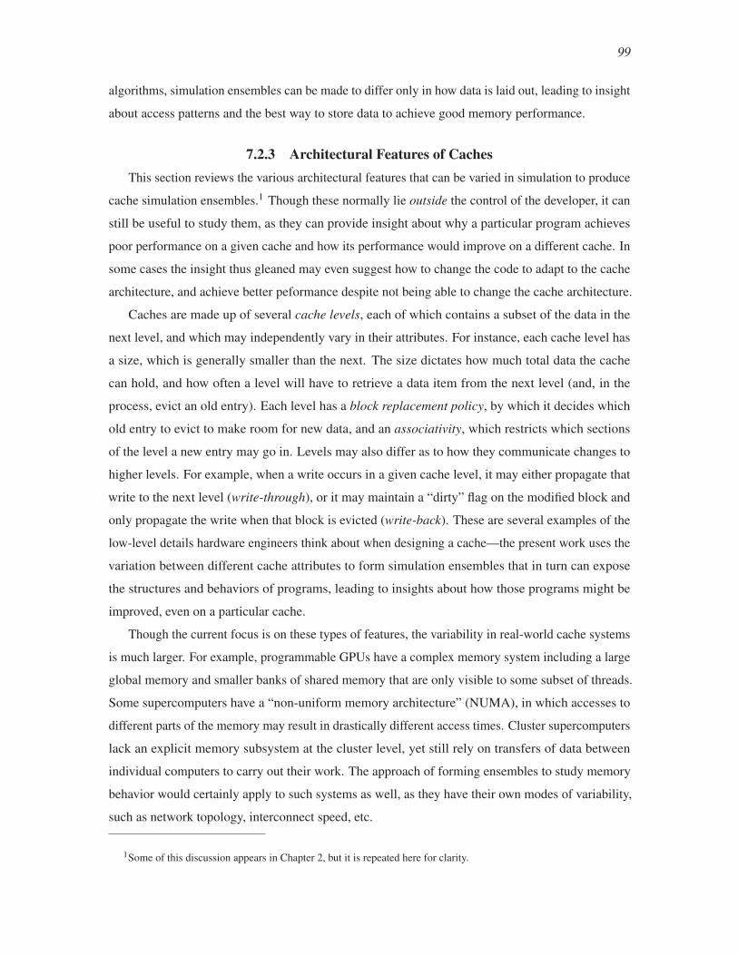
99
algorithms, simulation ensembles can be made to differ only in how data is laid out, leading to insight
about access patterns and the best way to store data to achieve good memory performance.
7.2.3 Architectural Features of CachesThis section reviews the various architectural features that can be varied in simulation to produce
cache simulation ensembles.1 Though these normally lie outside the control of the developer, it can
still be useful to study them, as they can provide insight about why a particular program achieves
poor performance on a given cache and how its performance would improve on a different cache. In
some cases the insight thus gleaned may even suggest how to change the code to adapt to the cache
architecture, and achieve better peformance despite not being able to change the cache architecture.
Caches are made up of several cache levels, each of which contains a subset of the data in the
next level, and which may independently vary in their attributes. For instance, each cache level has
a size, which is generally smaller than the next. The size dictates how much total data the cache
can hold, and how often a level will have to retrieve a data item from the next level (and, in the
process, evict an old entry). Each level has a block replacement policy, by which it decides which
old entry to evict to make room for new data, and an associativity, which restricts which sections
of the level a new entry may go in. Levels may also differ as to how they communicate changes to
higher levels. For example, when a write occurs in a given cache level, it may either propagate that
write to the next level (write-through), or it may maintain a “dirty” flag on the modified block and
only propagate the write when that block is evicted (write-back). These are several examples of the
low-level details hardware engineers think about when designing a cache—the present work uses the
variation between different cache attributes to form simulation ensembles that in turn can expose
the structures and behaviors of programs, leading to insights about how those programs might be
improved, even on a particular cache.
Though the current focus is on these types of features, the variability in real-world cache systems
is much larger. For example, programmable GPUs have a complex memory system including a large
global memory and smaller banks of shared memory that are only visible to some subset of threads.
Some supercomputers have a “non-uniform memory architecture” (NUMA), in which accesses to
different parts of the memory may result in drastically different access times. Cluster supercomputers
lack an explicit memory subsystem at the cluster level, yet still rely on transfers of data between
individual computers to carry out their work. The approach of forming ensembles to study memory
behavior would certainly apply to such systems as well, as they have their own modes of variability,
such as network topology, interconnect speed, etc.
1Some of this discussion appears in Chapter 2, but it is repeated here for clarity.
100
7.3 Visualizing Cache Simulation EnsemblesThis chapter focuses on directly comparing simulation results, varying some parameter or quality
of the simulations. Even with straightforward visualization for this comparison, valuable insights
about various case studies come about. The main approach is to plot a performance measure as a
function of time for all the ensemble members, on the same set of coordinate axes (resembling the
spaghetti plots of weather forecast ensemble visualization). Such a plot easily transmits the degree of
agreement or dispersion between the ensemble members, and also allows for quickly judging the
difference in performance between two or more ensemble members. Clustering, which indicates
relative insensitivity to the changing simulation parameters, is also easily visible.
The cache simulations work by first specifying a cache configuration and then feeding reference
trace records—which consist of a code indicating the type of access, such as “read” or “write,”
and the address of the transaction—one by one into it, allowing it to update its state and record
information about hits and misses. In particular, the simulated cache is able to report the level in
which requested data was found (for this purpose, main memory is treated as though it were another
level of cache). The resulting “hit level” data can be used for different visualization approaches, and
it is the focus of the work in this chapter.
7.3.1 EnsemblesThe hit level data can be weighted by time to yield a cache service time for that simulation step.
In other words, instead of directly plotting the hit level, a preset time-to-access is plotted for each
level instead. Typical values for a real-world cache might be three CPU cycles for L1 access, 15
cycles for L2, and a much larger 300 cycles for main memory. In the plots, each ensemble member is
represented by a curve showing this cache access time as a function of logical, or simulation time.
However, because caches are discrete systems, there is no natural continuity from one reference trace
record to the next, and as such the access time data can be very high-frequency as cache misses are
mixed in with cache hits. Because trends in the data are important, an averaging window is used to
collect several simulation steps’ results at each simulation time step, plotting a moving average of the
access times. Such low-pass filtering eliminates the obfuscating effect of individual, high-frequency
simulation steps coming together en masse. In this case, the y-axis more naturally has units of “cache
access time per memory access.”
The standard deviation within each averaging window can also be plotted over the data itself as
lighter-colored envelopes extending above and below the mean. This statistic is meant to capture
the high frequency activity hidden by the averaging window, but in practice, high-frequency activity
generally means more cache misses, which in turn inflates both the mean and the standard deviation,
due the high access time to main memory. The standard deviation is therefore a redundant encoding

101
of the information carried by the mean, and as such can help to visually reinforce the qualities of a
simulation ensemble (for example, in Figure 7.1). Alternatively, it can be useful to investigate the
general difference between ensemble members, as opposed to within a single member. In such cases,
the standard deviation of the member values is a measure of dispersion or disagreement among the
members.
When implemented as software, several aspects of the plotting process naturally fall under user
control, mediated by user interface elements. For instance, the size of the moving average window
can be changed at plotting time, giving users control over the smoothing effect of averaging and
allowing them to search for performance features at different scales. A focus-plus-context technique
(Figure 7.1(c)) allows for zooming in on a section of the graph while deemphasizing the remainder,
allowing for examination of details while still keeping a handle on the larger context.
7.3.2 Time MatchingWhen the ensembles differ in, for example, choice of algorithm, the ensemble members may
represent different numbers of total memory accesses. For example, Figure 7.3 compares bubble
and insertion sort. These have similar computational structure, but bubble sort engages in many
more memory accesses than insertion sort does. In order to effectively visualize the true differences
between the simulations, it may be necessary to transform them into a common timeframe in which
the comparison is easier. Throughout this dissertation, the program source code has served as a
familiar context. In this case, points in the source code at which the simulations are reaching the
same milestones can be identified—for instance, for bubble and insertion sort, one such point may
be the ends of the shrinking sweeps engaged in by the sorting algorithm. This casts the simulation
time into “source code time,” in which recurring lines of source code are taken as the main measure
of elapsed logical time. Figure 7.3 has vertical lines to indicate the ends of the sorting loops. The
insertion sort curve has been stretched to fit in the same timeframe as bubble sort (syncing up at
the vertical lines), which is reflected in the relative size of the color-coded circular glyphs at the
bottom. Because fewer simulation steps are represented by the insertion sort curve, it must also
have its average access time values scaled according to the difference in memory volume between
the simulations. This process is called time matching, and it is used to enforce common program
structure onto the simulation ensemble members so that comparisons between them are fair.
7.3.3 Visual DiffsWaxlamp (Chapter 5) can be extended to create a more specific method for comparing two
simulations differing only in their caches. Waxlamp visualizes a single trace by showing the flow of
individual data items between the levels of a simulated cache, visually highlighting cache misses and
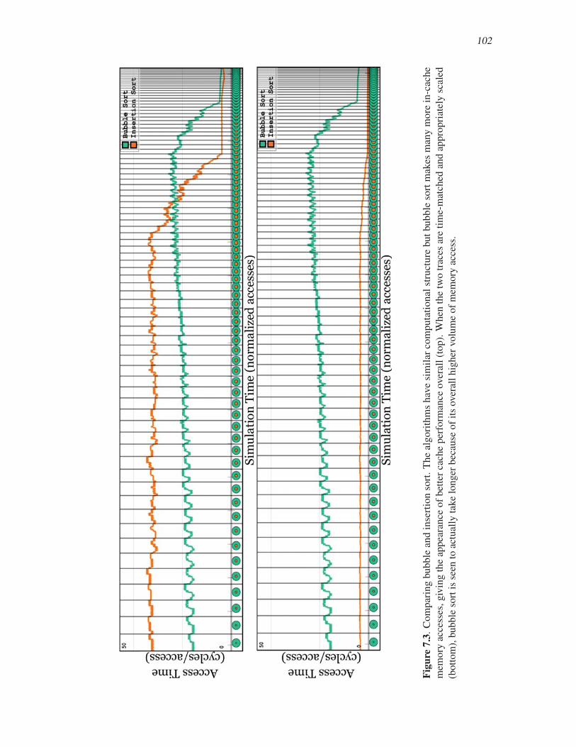
102
Figu
re7.
3.C
om
par
ing
bubble
and
inse
rtio
nso
rt.
The
algori
thm
shav
esi
mil
arco
mputa
tional
stru
cture
but
bubble
sort
mak
esm
any
more
in-c
ache
mem
ory
acce
sses
,g
ivin
gth
eap
pea
ran
ceo
fb
ette
rca
che
per
form
ance
over
all
(to
p).
Wh
enth
etw
otr
aces
are
tim
e-m
atch
edan
dap
pro
pri
atel
ysc
aled
(bott
om
),bubble
sort
isse
ento
actu
ally
take
longer
bec
ause
of
its
over
all
hig
her
volu
me
of
mem
ory
acce
ss.
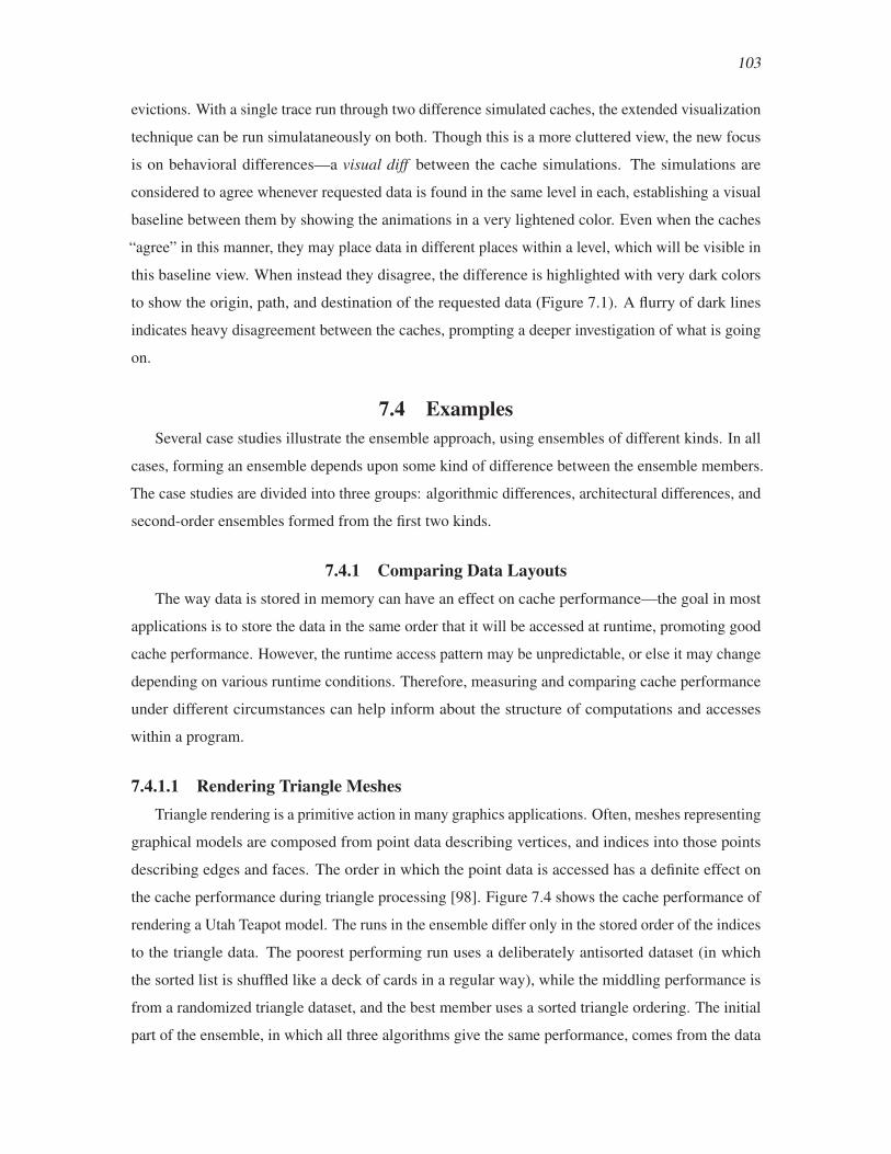
103
evictions. With a single trace run through two difference simulated caches, the extended visualization
technique can be run simulataneously on both. Though this is a more cluttered view, the new focus
is on behavioral differences—a visual diff between the cache simulations. The simulations are
considered to agree whenever requested data is found in the same level in each, establishing a visual
baseline between them by showing the animations in a very lightened color. Even when the caches
“agree” in this manner, they may place data in different places within a level, which will be visible in
this baseline view. When instead they disagree, the difference is highlighted with very dark colors
to show the origin, path, and destination of the requested data (Figure 7.1). A flurry of dark lines
indicates heavy disagreement between the caches, prompting a deeper investigation of what is going
on.
7.4 ExamplesSeveral case studies illustrate the ensemble approach, using ensembles of different kinds. In all
cases, forming an ensemble depends upon some kind of difference between the ensemble members.
The case studies are divided into three groups: algorithmic differences, architectural differences, and
second-order ensembles formed from the first two kinds.
7.4.1 Comparing Data LayoutsThe way data is stored in memory can have an effect on cache performance—the goal in most
applications is to store the data in the same order that it will be accessed at runtime, promoting good
cache performance. However, the runtime access pattern may be unpredictable, or else it may change
depending on various runtime conditions. Therefore, measuring and comparing cache performance
under different circumstances can help inform about the structure of computations and accesses
within a program.
7.4.1.1 Rendering Triangle MeshesTriangle rendering is a primitive action in many graphics applications. Often, meshes representing
graphical models are composed from point data describing vertices, and indices into those points
describing edges and faces. The order in which the point data is accessed has a definite effect on
the cache performance during triangle processing [98]. Figure 7.4 shows the cache performance of
rendering a Utah Teapot model. The runs in the ensemble differ only in the stored order of the indices
to the triangle data. The poorest performing run uses a deliberately antisorted dataset (in which
the sorted list is shuffled like a deck of cards in a regular way), while the middling performance is
from a randomized triangle dataset, and the best member uses a sorted triangle ordering. The initial
part of the ensemble, in which all three algorithms give the same performance, comes from the data

104
Figu
re7.
4.R
end
erin
gtr
ian
gle
sin
dif
fere
nt
ord
ers.
Ran
do
miz
edd
ata
(yel
low
)an
dan
adver
sesh
uffl
ing
(gre
en)
per
form
po
orl
y,w
ith
aro
ug
hly
fou
rfo
ld
impro
vem
ent
upon
sort
ing
the
dat
a(b
lue)
.
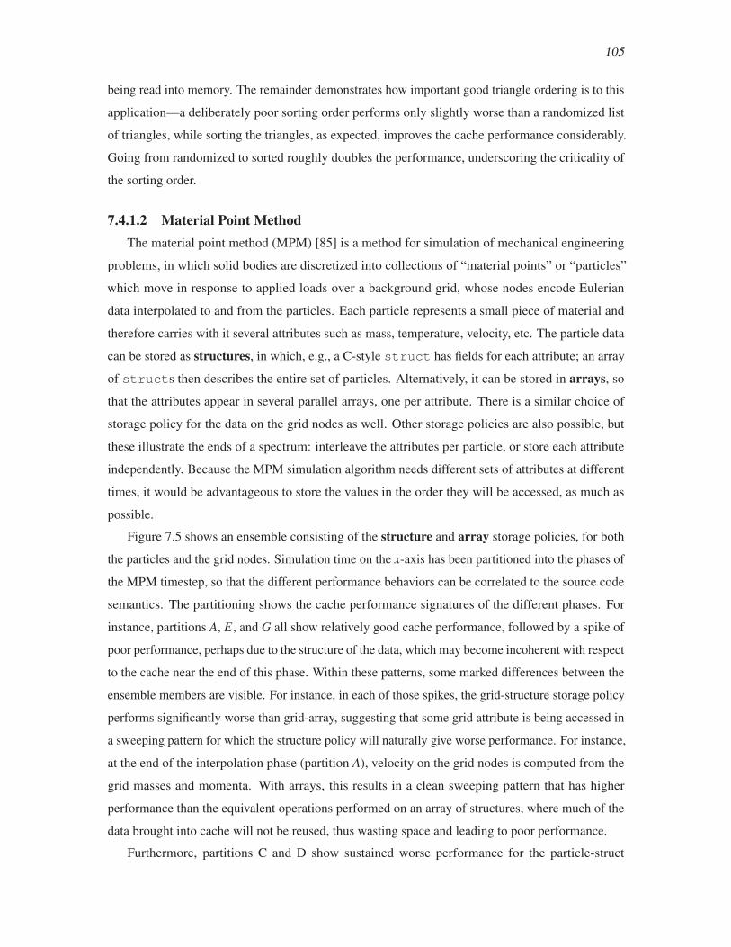
105
being read into memory. The remainder demonstrates how important good triangle ordering is to this
application—a deliberately poor sorting order performs only slightly worse than a randomized list
of triangles, while sorting the triangles, as expected, improves the cache performance considerably.
Going from randomized to sorted roughly doubles the performance, underscoring the criticality of
the sorting order.
7.4.1.2 Material Point MethodThe material point method (MPM) [85] is a method for simulation of mechanical engineering
problems, in which solid bodies are discretized into collections of “material points” or “particles”
which move in response to applied loads over a background grid, whose nodes encode Eulerian
data interpolated to and from the particles. Each particle represents a small piece of material and
therefore carries with it several attributes such as mass, temperature, velocity, etc. The particle data
can be stored as structures, in which, e.g., a C-style struct has fields for each attribute; an array
of structs then describes the entire set of particles. Alternatively, it can be stored in arrays, so
that the attributes appear in several parallel arrays, one per attribute. There is a similar choice of
storage policy for the data on the grid nodes as well. Other storage policies are also possible, but
these illustrate the ends of a spectrum: interleave the attributes per particle, or store each attribute
independently. Because the MPM simulation algorithm needs different sets of attributes at different
times, it would be advantageous to store the values in the order they will be accessed, as much as
possible.
Figure 7.5 shows an ensemble consisting of the structure and array storage policies, for both
the particles and the grid nodes. Simulation time on the x-axis has been partitioned into the phases of
the MPM timestep, so that the different performance behaviors can be correlated to the source code
semantics. The partitioning shows the cache performance signatures of the different phases. For
instance, partitions A, E, and G all show relatively good cache performance, followed by a spike of
poor performance, perhaps due to the structure of the data, which may become incoherent with respect
to the cache near the end of this phase. Within these patterns, some marked differences between the
ensemble members are visible. For instance, in each of those spikes, the grid-structure storage policy
performs significantly worse than grid-array, suggesting that some grid attribute is being accessed in
a sweeping pattern for which the structure policy will naturally give worse performance. For instance,
at the end of the interpolation phase (partition A), velocity on the grid nodes is computed from the
grid masses and momenta. With arrays, this results in a clean sweeping pattern that has higher
performance than the equivalent operations performed on an array of structures, where much of the
data brought into cache will not be reused, thus wasting space and leading to poor performance.
Furthermore, partitions C and D show sustained worse performance for the particle-struct
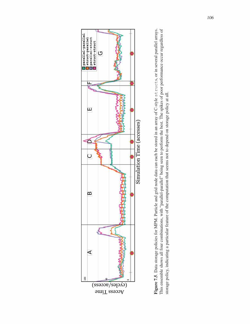
106
��
��
��
�
���������������� ������
����� �������� ��������
Figu
re7.
5.D
ata
sto
rag
ep
oli
cies
for
MP
M.P
arti
cle
and
gri
dn
od
ed
ata
can
each
be
sto
red
inan
arra
yo
fC
-sty
lestruct
s,o
rin
sever
alp
aral
lel
arra
ys.
Th
isen
sem
ble
show
sal
lfo
ur
com
bin
atio
ns,
wit
h“p
aral
lel-
par
alle
l”b
ein
gse
ento
per
form
the
bes
t.T
he
spik
eso
fp
oo
rp
erfo
rman
ceo
ccu
rre
gar
dle
sso
f
stora
ge
poli
cy,in
dic
atin
ga
par
ticu
lar
feat
ure
of
the
com
puta
tion
that
seem
snot
todep
end
on
stora
ge
poli
cyat
all.

107
policies. These phases, which have worse performance overall for all storage policies, perform
several matrix multiplications to carry out their work. The amplified difference between the array
and structure policies here reflects the cache difficulty of performing matrix multiplication to begin
with, complicated by the even poorer access patterns induced by structure storage. In fact, the
ensemble seems to show that parallel storage for both particle and grid data performs the best with
respect to the cache. Interestingly, this policy is not likely to be selected by the programmer, as it is
generally harder to juggle several parallel arrays than a single array of C-style structs—however,
this example clearly demonstrates how such a choice may lead to poor cache performance. One
solution is to abstract the details of how the data is accessed to behind a unified interface so that the
programmer may easily access data attributes without having to manage the arrays by hand, while
also achieving the better performance afforded by an array storage policy.
7.4.2 Comparing Algorithms
7.4.2.1 Bubble vs. Insertion SortFigure 7.3 compares bubble and insertion sort, which have similar computational structure, but
use memory differently. Both make repeated, shrinking sweeps of the list to be sorted, leaving the
largest of the remaining elements in its correct position at the end of each sweep. However, bubble
sort uses many more write operations than insertion sort does, as it uses repeated swaps to move
elements, whereas insertion sort only performs a single swap per sweep to move the largest element
into place. In the Waxlamp discussion (Chapter 5), it was noted that while bubble sort appears to
have much better cache performance than insertion (because all of its extra writes result in cache
hits), insertion sort may actually have better performance simply because it performs fewer memory
accesses overall.
In Figure 7.3, the traces have been time-matched to the ends of their sweep operations (top), with
attendant scaling of the average access times (bottom). When accounting for bubble sort’s extra
memory accesses, it can be seen that insertion sort has better memory performance overall. This
analysis demonstrates how a simple report of “cache hit rates” may be misleading when comparing
alternate approaches that compute the same result.
7.4.2.2 Matrix MultiplicationMatrix multiplication is an important operation in many scientific programs. Its memory behavior
is therefore of concern to high-performance scientific software developers. The naive algorithm
for matrix multiply computes dot products of the rows of the left-hand matrix and columns of the
right-hand matrix, introducing a cache-unfriendly access pattern for the latter (since the elements of
a single column do not reside in the same cache block, inducing several cache misses when accessing
108
the elements of the column). A simple solution is to store the right-hand matrix in column-major
order, transposing its access pattern to a cache-friendly one. Figure 7.6(a) shows that the “transposed
multiply” has dramatically better cache performance.
However, a column-major right-hand matrix means that it cannot be used as the left-hand matrix
in a different multiplication without once more causing poor access patterns. The more general
cache-friendly solution is to use matrix blocking, in which submatrices are repeatedly multiplied,
accumulating their products into submatrices of the final result. The block sizes are chosen so they
fit into cache, improving the reuse of the appropriate entries. Figure 7.6(a) also shows the relative
performance of blocked matrix multiply compared to the naive algorithm. Interestingly enough,
these results show that blocking performs worse than the transposed multiply. This is puzzling and
counterintuitive, as blocking is known to be an efficient technique for matrix multiplication.
Reduced associativity in caches accelerates the block eviction process, but restricts where
incoming blocks may go. When a program’s access patterns show certain kinds of regularity, the
cache may perversely end up using a limited number of its associative sets exclusively, leaving others
idle, and leading to an increased miss rate. In fact, exactly this behavior occurs in the blocked matrix
multiplcation example above. The example uses a 16×16 matrix, with blocks of size 4×4, giving the
starting address of each block the same modulo-4 address, thereby causing the start of every block
to map to the same associative set in any cache using four sets (as the simulated cache does in this
case), roughly quadrupling the miss rate, and slashing performance in half (Figure 7.6(b)).
The visualization and analysis suggest a simple fix: to stagger the mapped sets in each block of
the matrix, simply insert some amount of padding after the storage for each row. With rows of 16
elements, amounts of padding from 0 to 15 excess elements per row are possible. Studying how much
padding to use in this case is a prime example of the usefulness of cache ensembles—Figure 7.6(c)
includes an ensemble member for each of the 16 options. Figure 7.6(d-f) shows differential versions
of Figure 7.6(c), each one subtracting out a particular curve from all the ensemble members, allowing
for direct comparision of value. As expected, a padding of two elements does a better job of
staggering the block addresses than a padding of four. Padding with six extra elements does even a
better job of redistributing the addresses throughout the sets of the cache, and seems to be the best
solution in this case.
7.4.3 Cache Size and Working SetsThe size of a cache is a very important parameter—generally speaking, a larger cache suffers
fewer cache misses, due to less contention for space. Simulation ensembles in which the cache
size varies can be used to expose the size of the working set of an application, the total amount of
memory the application requires during a given phase of its run. For example, consider the ensemble

109
Figure 7.6. Cache performance analysis of matrix multiplication. (a) The naive algorithm (orange)
performs the worst, due to cache-unfriendly access patterns. The other members show different
algorithms with better performance, but surprisingly, the well-known blocked multiply algorithm
does not perform as well as expected. (b) This ensemble shows the effect of cache associativity on
block matrix multiplication, accounting for the lost performance. (c) Different amounts of padding
inserted at the ends of the matrix rows help redistribute cache activity around the associative sets,
alleviating the loss in performance. (d-f) The same data appearing in (c), but with the curves for
padding amounts of two, four, and six subtracted uniformly out, respectively. A padding amount of
six seems to offer near-optimal gains.

110
(a)
Nai
ve,
tran
spose
d,an
dblo
cked
mat
rix
mult
iply
.

111
(b)
The
effe
ctof
cach
eas
soci
ativ
ity
on
blo
cked
mat
rix
mult
ipli
cati
on.
(Fig
ure
7.6,
con’
t)
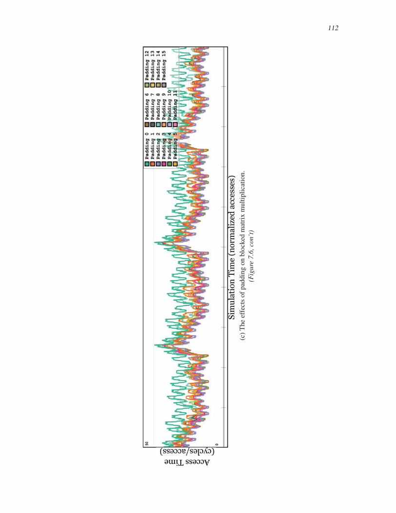
112
(c)
The
effe
cts
of
pad
din
gon
blo
cked
mat
rix
mult
ipli
cati
on.
(Fig
ure
7.6,
con’
t)

113
(d)
Dif
fere
nti
alvie
ww
ith
pad
din
gof
two.
(Fig
ure
7.6,
con’
t)
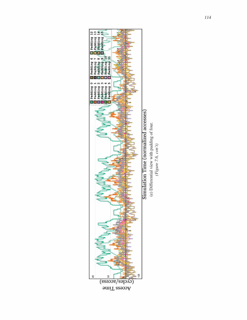
114
(e)
Dif
fere
nti
alvie
ww
ith
pad
din
gof
four.
(Fig
ure
7.6,
con’
t)

115
(f)
Dif
fere
nti
alvie
ww
ith
pad
din
gof
six.
(Fig
ure
7.6,
con’
t)
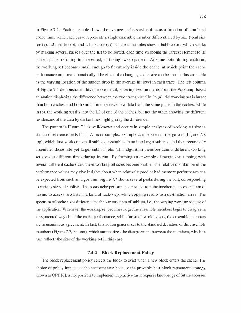
116
in Figure 7.1. Each ensemble shows the average cache service time as a function of simulated
cache time, while each curve represents a single ensemble member differentiated by size (total size
for (a), L2 size for (b), and L1 size for (c)). These ensembles show a bubble sort, which works
by making several passes over the list to be sorted, each time swapping the largest element to its
correct place, resulting in a repeated, shrinking sweep pattern. At some point during each run,
the working set becomes small enough to fit entirely inside the cache, at which point the cache
performance improves dramatically. The effect of a changing cache size can be seen in this ensemble
as the varying location of the sudden drop in the average hit level in each trace. The left column
of Figure 7.1 demonstrates this in more detail, showing two moments from the Waxlamp-based
animation displaying the difference between the two traces visually. In (a), the working set is larger
than both caches, and both simulations retrieve new data from the same place in the caches, while
in (b), the working set fits into the L2 of one of the caches, but not the other, showing the different
residencies of the data by darker lines highlighting the difference.
The pattern in Figure 7.1 is well-known and occurs in simple analyses of working set size in
standard reference texts [41]. A more complex example can be seen in merge sort (Figure 7.7,
top), which first works on small sublists, assembles them into larger sublists, and then recursively
assembles those into yet larger sublists, etc. This algorithm therefore admits different working
set sizes at different times during its run. By forming an ensemble of merge sort running with
several different cache sizes, these working set sizes become visible. The relative distribution of the
performance values may give insights about when relatively good or bad memory performance can
be expected from such an algorithm. Figure 7.7 shows several peaks during the sort, corresponding
to various sizes of sublists. The poor cache performance results from the incoherent access pattern of
having to access two lists in a kind of lock-step, while copying results to a destination array. The
spectrum of cache sizes differentiates the various sizes of sublists, i.e., the varying working set size of
the application. Whenever the working set becomes large, the ensemble members begin to disagree in
a regimented way about the cache performance, while for small working sets, the ensemble members
are in unanimous agreement. In fact, this notion generalizes to the standard deviation of the ensemble
members (Figure 7.7, bottom), which summarizes the disagreement between the members, which in
turn reflects the size of the working set in this case.
7.4.4 Block Replacement PolicyThe block replacement policy selects the block to evict when a new block enters the cache. The
choice of policy impacts cache performance: because the provably best block repacment strategy,
known as OPT [6], is not possible to implement in practice (as it requires knowledge of future accesses
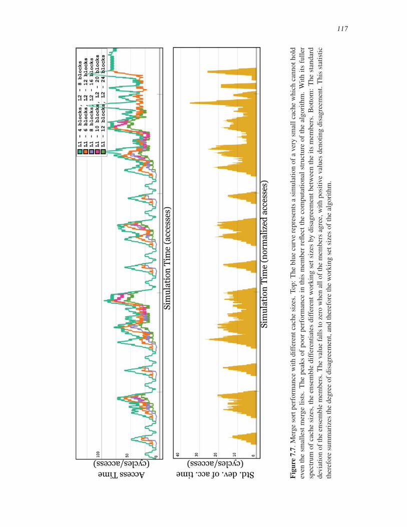
117
Figu
re7.
7.M
erg
eso
rtp
erfo
rman
cew
ith
dif
fere
nt
cach
esi
zes.
To
p:
Th
eb
lue
curv
ere
pre
sen
tsa
sim
ula
tio
no
fa
ver
ysm
all
cach
ew
hic
hca
nn
ot
ho
ld
even
the
smal
lest
mer
ge
list
s.T
he
pea
ks
of
poor
per
form
ance
inth
ism
ember
refl
ect
the
com
puta
tional
stru
cture
of
the
algori
thm
.W
ith
its
full
er
spec
trum
of
cach
esi
zes,
the
ense
mble
dif
fere
nti
ates
dif
fere
nt
work
ing
set
size
sby
dis
agre
emen
tbet
wee
nth
eit
sm
ember
s.B
ott
om
:T
he
stan
dar
d
dev
iati
on
of
the
ense
mble
mem
ber
s.T
he
val
ue
fall
sto
zero
when
all
of
the
mem
ber
sag
ree,
wit
hposi
tive
val
ues
den
oti
ng
dis
agre
emen
t.T
his
stat
isti
c
ther
efore
sum
mar
izes
the
deg
ree
of
dis
agre
emen
t,an
dth
eref
ore
the
work
ing
set
size
sof
the
algori
thm
.

118
at eviction time), an implementable approximation must be used instead.2 A commonly used policy
is known as least-recently used (LRU), in which the least recently accessed block is evicted. LRU
works well in practice, and is so common that Hill’s groundbreaking work on analysis of caches
and cache behavior [42], assumes it as a base feature of caches. However, there are cases where
LRU is not the best policy due to the structure of computations. By forming simulation ensembles
in which the replacement policy varies, it is possible to see the effect of different policies on the
miss rate of a program. In general, OPT and its inverted, pessimal counterpart PES (which evicts the
soonest-needed block, to cause as many replacement misses as possible) bound the performance of
replacement policies, giving some idea of how much damage could be caused by the replacement
policy.
Figure 7.8(top) shows an interesting example of a case in which LRU may not be the best option.
The program in this case is a heat equation solver that uses finite differences to repeatedly sweep a
data array, updating it with the time-changing solution to produce several timesteps worth of data.
For repeated sweeps of this type, most-recently used (MRU) is the optimal replacement strategy [15].
Figure 7.8 bears this out, as the ensemble member for the MRU cache closely matches that of the
OPT cache.
However, as mentioned before, the replacement strategy is out of the control of the developer.
This means the heat equation solver is stuck with LRU, but the analysis suggests a possible corrective
course of action. The trouble with LRU is that it tends to evict blocks that will be needed in the near
future—if we were to reverse the order of updates periodically, we could try to “trick” LRU into
behaving more like MRU. The program can be modified to use “pingpong” sweeps, proceeding first
from the first element to the last, then making the next sweep from last to first, and then repeating. By
reversing the direction at intervals, LRU now tends to throw out blocks that will be needed furthest in
the future. Figure 7.8 (bottom) shows that LRU with the pingpong strategy performs as well as MRU
did with the original program. In other words, an optimal setting has been found, under the constraint
of having to use LRU in the cache. This is a case where investigating the possibilities—even when
they are out of reach in practice—led to a vastly improved practical solution.
7.4.5 Second-Order EnsemblesIt is also possible to combine members of an existing ensemble in meaningful ways to yield
a new, second-order ensemble, that offers its own insights about program behavior. Consider the
ensemble of varying cache sizes in Figure 7.1. As discussed previously, this ensemble says something
2Because the full reference trace is available, there is sufficient knowledge of “the future” to implement OPT and PES
for simulated caches.
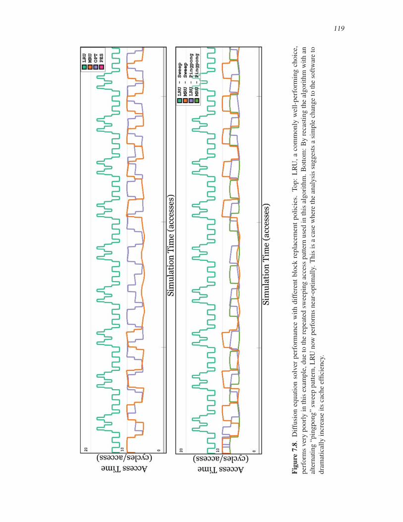
119
Figu
re7.
8.D
iffu
sion
equat
ion
solv
erper
form
ance
wit
hdif
fere
nt
blo
ckre
pla
cem
ent
poli
cies
.T
op:
LR
U,
aco
mm
only
wel
l-per
form
ing
choic
e,
per
form
sver
ypoorl
yin
this
exam
ple
,due
toth
ere
pea
ted
swee
pin
gac
cess
pat
tern
use
din
this
algori
thm
.B
ott
om
:B
yre
cast
ing
the
algori
thm
wit
han
alte
rnat
ing
“pin
gp
on
g”
swee
pp
atte
rn,
LR
Un
owp
erfo
rms
nea
r-o
pti
mal
ly.
Th
isis
aca
sew
her
eth
ean
aly
sis
sug
ges
tsa
sim
ple
chan
ge
toth
eso
ftw
are
to
dra
mat
ical
lyin
crea
seit
sca
che
effi
cien
cy.
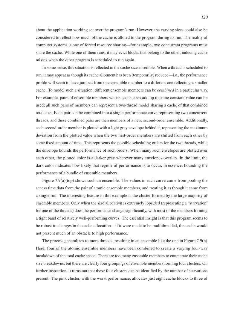
120
about the application working set over the program’s run. However, the varying sizes could also be
considered to reflect how much of the cache is alloted to the program during its run. The reality of
computer systems is one of forced resource sharing—for example, two concurrent programs must
share the cache. While one of them runs, it may evict blocks that belong to the other, inducing cache
misses when the other program is scheduled to run again.
In some sense, this situation is reflected in the cache size ensemble. When a thread is scheduled to
run, it may appear as though its cache allotment has been (temporarily) reduced—i.e., the performance
profile will seem to have jumped from one ensemble member to a different one reflecting a smaller
cache. To model such a situation, different ensemble members can be combined in a particular way.
For example, pairs of ensemble members whose cache sizes add up to some constant value can be
used; all such pairs of members can represent a two-thread model sharing a cache of that combined
total size. Each pair can be combined into a single performance curve representing two concurrent
threads, and these combined pairs are then members of a new, second-order ensemble. Additionally,
each second-order member is plotted with a light gray envelope behind it, representing the maximum
deviation from the plotted value when the two first-order members are shifted from each other by
some fixed amount of time. This represents the possible scheduling orders for the two threads, while
the envelope bounds the performance of such orders. When many such envelopes are plotted over
each other, the plotted color is a darker gray wherever many envelopes overlap. In the limit, the
dark color indicates how likely that regime of performance is to occur, in essence, bounding the
performance of a bundle of ensemble members.
Figure 7.9(a)(top) shows such an ensemble. The values in each curve come from pooling the
access time data from the pair of atomic ensemble members, and treating it as though it came from
a single run. The interesting feature in this example is the cluster formed by the large majority of
ensemble members. Only when the size allocation is extremely lopsided (representing a “starvation”
for one of the threads) does the performance change significantly, with most of the members forming
a tight band of relatively well-performing curves. The essential insight is that this program seems to
be robust to changes in its cache allocation—if it were made to be multithreaded, the cache would
not present much of an obstacle to high performance.
The process generalizes to more threads, resulting in an ensemble like the one in Figure 7.9(b).
Here, four of the atomic ensemble members have been combined to create a varying four-way
breakdown of the total cache space. There are too many ensemble members to enumerate their cache
size breakdowns, but there are clearly four groupings of ensemble members forming four clusters. On
further inspection, it turns out that these four clusters can be identified by the number of starvations
present. The pink cluster, with the worst performance, allocates just eight cache blocks to three of
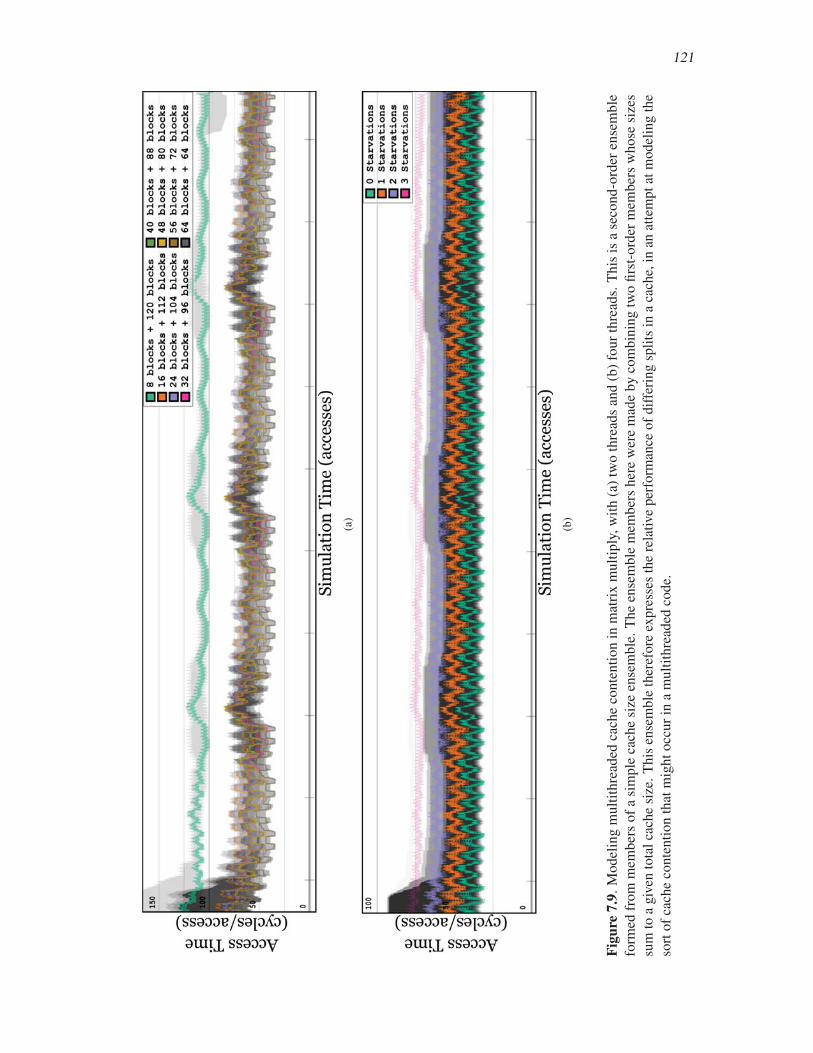
121
(a)
(b)
Figu
re7.
9.M
odel
ing
mult
ithre
aded
cach
eco
nte
nti
on
inm
atri
xm
ult
iply
,w
ith
(a)
two
thre
ads
and
(b)
four
thre
ads.
This
isa
seco
nd-o
rder
ense
mble
form
edfr
om
mem
ber
so
fa
sim
ple
cach
esi
zeen
sem
ble
.T
he
ense
mble
mem
ber
sher
ew
ere
mad
eby
com
bin
ing
two
firs
t-o
rder
mem
ber
sw
ho
sesi
zes
sum
toa
giv
ento
tal
cach
esi
ze.
Th
isen
sem
ble
ther
efo
reex
pre
sses
the
rela
tive
per
form
ance
of
dif
feri
ng
spli
tsin
aca
che,
inan
atte
mp
tat
mo
del
ing
the
sort
of
cach
eco
nte
nti
on
that
mig
ht
occ
ur
ina
mult
ithre
aded
code.
122
the threads, allowing the rest of the cache to the fourth. Similarly, the blue cluster allocates two such
small threads, the orange cluster only one, and the green cluster represents the optimal case where no
single thread receives such a small allocation. It may seem obvious that starving a single thread leads
to poor performance, but the real insight in this example is the stability of performance with respect
to such extreme allocations. As long as no thread receives the minimal amount of allocation, the
performance for all other combinations remains in a narrow band, which in turn indicates a kind of
cache stability.
This is just one example of a higher-order ensemble that can be used to model and reason about
more complex behaviors possible within computer systems. It is not meant to be an accurate model
of the actual execution of such a behavior, but rather a way to reason about what might be expected
of, for instance, cache performance, when such execution is set up. It is remarkable that a model
of concurrent multithreaded execution can be formed using data from a single-threaded run, and it
therefore suggests that other complex systems behavior might be modellable from such data. This is
one major directions of future inquiry, as being able to predict or model complex behavior from a
relatively simple trace would be a major advance in processing this kind of data, and would likely
generalize to many types of computing platforms.
7.5 ConclusionsThis chapter demonstrates an approach to investigating cache performance uncertainty and varia-
tion by using cache simulation ensembles and techniques from information visualization to display
them. The major approach is to plot performance metrics with an eye towards highlighting specific
instances of general patterns. By varying different features, different behavior and performance
characteristics become visible. The case studies clearly show some surprising results in unexpected
places, as well as suggest practicable solutions to such problems where they arise.
One major avenue of future work lies in refining and improving the ideas about modeling
multicore execution. Though the model presented in this chapter is not meant to be accurate, it will
be useful to confirm some of the findings about, for example, robustness of multicore programs to
varying cache allocation. Another area of future work is in designing specific visual encodings for
the various types of patterns that have arisen in the case studies. It is promising that just with basic
information visualization techniques, some insight about program behavior and performance arise;
with dedicated, pattern-specific visualization solutions, the methods are expected to become even
more useful.
Uncertainty analysis has turned out to be an illuminating approach to cache performance analysis,
suggesting new ways to think about program performance behavior, leading to hopefully more and
more insights that will help design more effective programs, increasing their value.

CHAPTER 8
DISCUSSION
This chapter discusses some of the interesting interactions that arise when considering the work
presented in the preceding chapters within a larger context. Briefly, the topics of discussion are
as follows: a comparison of MTV and Waxlamp, since both approaches deal with visualizing
reference trace data directly, albeit in different ways; the issue of handling the time dimension, an
integral part of a reference trace; a comparison of MTV and Waxlamp with the topological and
ensemble approaches, since the former are “animation” techniques and the latter “static;” and finally,
a discussion of the user interface features described for MTV, and how these might be generalized to
the other approaches presented.
8.1 MTV vs. WaxlampMTV (Chapter 4) and Waxlamp (Chapter 5) were the first two works presented in this dissertation,
both dealing with reference traces in a similar fashion: treating them as records of events, then
“playing them back” over appropriately designed visual structures. Both approaches make heavy use
of animation to move from event to event within the trace (a topic that is treated in its own right
below). Aside from this basic setup, however, the approaches are very different, using different visual
preparations, focusing on different aspects of the traces, and delivering different classes of insights.
MTV was billed as a simpler approach, without the use of heavier visual metaphors, and minimal
filtering of the data, instead opting to allow the user to select some ranges of addresses of interest,
and then driving the visualization with a display of item access in the order they occurs, along with a
visualization of cache block residency and cache performance. MTV’s greatest strength, therefore, is
its ability to cleanly show the access patterns encoded in the trace. These can be useful for verifying
“healthy” access patterns within some algorithm, or, more generally, finding out when a program’s
cache coherency disappears due to poor access patterns. Essentially, MTV visualizes a quality of
memory access that is widely discussed, and even taught to first-year students, but that cannot often
be seen directly without the aid of such a system.
124
By contrast, Waxlamp concerns itself much less with the concrete access patterns that are MTV’s
speciality, instead focusing on the contents of the cache in an abstract manner, showing how each
event causes changes to the ranks of data stored in the cache. Though both systems highlight
important performance events such as cache misses, Waxlamp does so by tagging some type of data
motion event with a salient color to draw the eye to the otherwise mundane event being depicted. In
some sense, Waxlamp takes the fundamental visual structures of MTV, wraps them into a new shape,
and adds data motion information. In doing so, Waxlamp presents a busier, richer display; however,
the strength of MTV’s concrete access pattern visualization is downplayed in Waxlamp, as a volume
of other visual events comes to the forefront. This relationship reflects the anecdotal response of
colleagues to a demonstration of Waxlamp: overwhelmingly, people who previously acknowledged
the usefulness and novelty of MTV have reacted by preferring Waxlamp, even with its busier view.
In summary, it might be said that MTV is a system designed to generalize and extend the kinds of
static diagrams used to visualize memory access models in introductory textbooks (e.g., [41]) and
is perhaps well-suited for educational purposes; by contrast, Waxlamp is instead a more flexible
generalization of MTV—and with its notion of a specifically designed static structure against which
to play back trace data, it also suggests a framework for performing event trace visualization in
general.
Since MTV’s strength in displaying access patterns concretely is something that doesn’t com-
pletely survive in Waxlamp, the systems have distinct sets of strengths and weaknesses and it may
pay to think about ways the features of each system might cross-pollinate to produce greater overall
value (Figure 8.1). For example, MTV has the ability to reformat a bare data array into a higher-level
structure (such as a two-dimensional array). Waxlamp retains MTV’s notion of displaying access
patterns by keeping ghostly data glyphs in the outermost ring, representing the original data array
in memory. As events from the trace play back, these ghostly glyphs are affected, and the access
patterns are visible to some degree. Possibly, the space outside of this outer ring could be used to
display MTV-style reformatted data arrays, in order to display the higher-order structural information
as well.
MTV also displays a persistent indicator of the “cache result” a particular reference had on its last
access—i.e., hit to L1, hit to L2, or miss. Similarly, it might be useful to include such an indicator in
the outer ring of the Waxlamp display, to give another persistent marker for the history of behavior
encoded in the trace. Waxlamp’s general mode of operation displays a lot of activity from moment to
moment, with history visible as fading pathlines into the past, so another, more persistent feature of
history might bolster the viewer’s sense of context as the trace plays back.
Finally, Waxlamp’s major extension over MTV is the idea of display data motion within the

125
(a) (b) (c) (d)
Figure 8.1. A review of features of MTV and Waxlamp. (a) MTV can format bare arrays into
higher-order structures such as two-dimensional arrays. (b) MTV also shows a persistent indicator of
the result some access had in the cache (red/blue/magenta color elements in lower portions of each
cell). (c) Finally, MTV shows just the cache block residency, color coded by region of origin. (d)
Waxlamp focuses largely on data motion between levels of the cache. The features shown in (a) and
(b) are not present in Waxlamp; perhaps the space outside the outermost ring could be used to import
these features, to promote deeper understanding of the memory behavior. Similarly, MTV’s static
display of the cache contents could benefit from using a simplified version of Waxlamp’s data motion
model, using animation to express the state-to-state changes in the cache.
levels of the simulated cache. MTV’s cache visualization sticks to simple cache block residency,
with the idea that cache contention might be visible as rapidly changing colors within some region
of a cache level. If a visualization of data motion were used instead—to show not just cache block
residency, but the manner in which that residency changes—then perhaps the cache visualization
could be more effective.
8.2 Handling the Time DimensionTime is a critical dimension of reference trace data: the events are ordered in history, and this
order matters to the outcome of processes such as cache simulation and the visualization of the events
themselves. In terms of visualization, there are two major ways of encoding the time dimension
visually: these might be called time-for-time and space-for-time. A time-for-time encoding matches
up the passing of time within the data stream with the passing of time in the visualization—that
is, it uses animation. This is the approach used by both MTV and Waxlamp. On the other hand, a
space-for-time encoding treats some spatial dimension of the visualization space as representing
time; then, events plotted along this spatial dimension will be seen as going forward in time. The
topological and ensemble approaches both use this type of encoding. For example, as the nodes of
the topological parameterizations spiral outwards (Chapter 6), they go forward in time, thus treating
the radius of a circular display as a measure of time. More traditionally, the plots used to examine
the cache simulation ensembles (Chapter 7) place time on the x-axis, encoding the passage of time
into rightward motion on the display.

126
Therefore, in MTV and Waxlamp, events are displayed “as they occur”—the viewer is allowed
to fully investigate all of the complex state associated with a particular moment, and to see this
state morph into the next state as a new event plays back. Some amount of history is visible, either
as a fading trail of previous activity (as in MTV), or as a series of fading pathlines reaching into
the past (as for Waxlamp), serving as temporal context for the viewer. By contrast, the topology
and ensemble approaches show history on the whole, allowing the viewer to see trends in activity
across longer stretches of time, constituting a longer perspective from which to view reference trace
activity. However, in such views it is much more difficult to show the range of information that can
be displayed in an animation view, since generally only a single spatial dimension is available for
representing the flow of time. This represents a basic tradeoff between the visibility of detail and
scope.
As both approaches to handling time have advantages and disadvantages, it may be valuable to
combine the approaches, trying to deliver the best of both worlds while mitigating the drawbacks
of each. MTV already features one example of this approach: it includes a “cache event map” as
described by Yu et al. [99] that has been made clickable, transporting the user to a particular moment
in the trace. The map itself is a space-for-time encoding of the cache activity, which each pixel in the
image showing whether the cache hit or missed at a given reference trace record; these pixels are laid
out in a one-dimensional ordering reflecting the passage of time. MTV features the cache event map
as a way to select a moment in time to visit at a glance and a click, deepening the user’s navigation
context. Such an approach would also be useful in Waxlamp, including the use of the topological
and ensemble visualizations presented in this dissertation in lieu of, or in addition to, the cache event
map.
Going the other direction, it would also be interesting to call up a snippet of an animation-based
visualization in response to a user click on some portion of the static topology- or ensemble-based
visualization. This would be a drill-down technique for layering the richer animation-approach-based
detail over a static display upon request.
8.3 Summary of Visual BehaviorsThroughout the presentation and discussion of the four visualization approaches in this disserta-
tion, many visual features have been described as comprising each approach. This section discusses
these features at a slightly higher level: in terms of healthy and unhealthy memory behaviors. Healthy
memory behaviors are, by definition, any behaviors that lead to a high cache hit rate; unhealthy
behaviors, by contrast, are those that do not. Of course, how healthy a particular behavior is depends
on the cache being simulated; however, this section speaks about the visual effects observed in each

127
of the approaches for both healthy and unhealthy behavior. Some examples of healthy behaviors are
sweeping access patterns for updating values, accessing data when it lies in cache, using nearby data
soon after it enters the cache, and performing the maximum amount of computation with data that is
resident in the cache.
Alternatively, this section represents something of a catalogue of visual behaviors to look for
when using the visualization approaches to investigate memory behavior.
8.3.1 MTVThe major mark of healthy memory behavior in MTV is a glowing cache, indicating high cache
temperature and therefore a high hit rate. Such behaviors will also produce many blue lights in the
bottom portion of each access, indicating cache hits.
As MTV’s main strength is in concretely displaying the shape of access patterns, sweeping access
patterns are especially salient in MTV. These appear as a moving, fading trail of accesses across the
array glyphs, concretely representing a “sweep.” Such a pattern results in a single cache miss for a
new block of data, followed immediately by several cache hits, causing the L1 cache level to glow
white-hot. If the array region represents a two-dimensional array, the 2D glyph will show a row-major
access pattern, confirming the common wisdom of what such a healthy pattern should look like.
Examples of healthy behaviors with these visual characteristics include several examples discussed
in Chapter 4, such as the “good stride” example that simply sweeps across an array, blocked matrix
multiplication, and material point method (MPM) using parallel arrays.
By contrast, unhealthy behaviors will lead to exactly the opposite visual behaviors. Access
patterns will decohere, showing random or otherwise “jumpy” behavior spread out over the glyph,
with little or no sense of contiguity. These will tend to leave the cache cold, and produce more cache
misses, visible as a higher volume of red cache indicator lights. The “bad stride” access example
from Chapter 4, as well as naive matrix multiplication, and MPM with structs all exemplify unhealthy
behaviors as they appear in MTV.
8.3.2 WaxlampBy constrast with MTV, Waxlamp focuses on data motion within the cache, and visual represen-
tations of the attendant cache events, such as hits and misses. As such, visual behaviors of healthy
and unhealthy behaviors in Waxlamp manifest mainly via the volume of hit and miss activity in the
cache. Healthy behaviors will cause the cache levels to glow red, indicating high temperature, along
with heavy volume of access activity within the cache levels. Cache misses will be minimal, with
conspicuous lack of data motion from the outer main memory ring. Sweeping patterns are seen to
do well in Waxlamp for a different reason than in MTV: once the initial cache miss brings data into

128
cache, Waxlamp shows nearby data being accessed subsequently, resulting in a pattern of intermittent
cache misses punctuated by frantic activity within the L1 cache level. In general, frantic activity
inside the cache itself is a sign of healthy behavior.
In addition to the cache hit and miss activity, the sweeping pattern shows another visual
characteristic: since data in a sweep is accessed only once, data will enter the cache, be accessed,
and then slowly slip out of L1 as it is pushed out toward the ends of the associative set spiral arms,
falling out to L2 and then repeating the slipping action until it is evicted back out to main memory.
Generalizing this pattern, an even healthier behavior would be one in which data does not slip out of
L1 after a single access, but is instead repeatedly pulled to the center of the display by subsequent
accesses before it can “escape” to L2 and then main memory, resulting in higher L1 hit rates. Some
examples of healthy behaviors displayed in Waxlamp include the latter stages of a bubble sort
computation, as well as the earlier, small working set stages of merge sort.
Unhealthy behaviors lead instead to blue-glowing cache, indicating a low temperature, and many
cache misses, indicated by a heavy volume of long red trails moving quickly from the outer ring to
the center of the display. The earliest stages of bubble sort, as well as the larger working set phases
of merge sort exemplify such poor behaviors.
Finally, Waxlamp is able to visualize some behaviors related to associativity. In particular, when
accesses are not well-aligned and tend to alias to only a subset of the associative sets, this will be
visible as activity occurring only in some of the sets while other sets lie dormant. Such behavior is
unhealthy because it effectively lowers the size of the cache, inducing many more cache misses than
with a more balanced associative behavior. When such accesses are balanced, they will be visible as
activity distributed relatively equally among the associative sets, perhaps with a particular type of
pattern, such as subsequent accesses going to different sets, wheeling about the center of the display.
One example of such behavior is the misaligned blocked matrix multiply discussed in Chapter 7.
8.3.3 TopologyBecause the topology-based visualization approach is not at all driven by cache simulation, the
usual notions of healthy and unhealthy behavior do not apply here. The strength of the topology
approach is to illustrate recurrent behavior within the trace itself. Since recurrence in the trace can
represent either healthy or unhealthy behavior, a different approach is needed to find interesting
information in the topology-based visualizations.
One example of a possible unhealthy behavior indicated by the topological visualization is
the case in which tightly repeated recurrences occurring very quickly in time can indicate wasted
computation or memory access. Figure 6.10(a) shows a possible example. Here, each invocation of
the shape function S() results in two very tightly couple iterations in the image. Further inspection

129
reveals that the function S() simply defers to two one-dimensional shape functions S x() and
S y(), each of which performs an identical sequence of actions, differing only in values of the
parameters. It may occur to the programmer that, while using two one-dimensional functions
with different names may be a nice abstraction to rely on, it seems to result in the same memory
locations being loaded twice in sequence. If the second batch of extra memory activity, and attendant
computation, could be avoided, and both one-dimensional shape values computed upon a single
loading of the needed data, then perhaps the computation of the overall shape function S() could be
sped up.
In this case, the visualization brings a curious feature of the runtime computation to the attention
of the programmer, who may then use knowledge of the code base to reason about why that feature
is appearing in the visualization. While this does not guarantee a viable optimization, it does suggest
a place where the programmer can look for one.
8.3.4 EnsembleFinally, the ensemble approach, relying mainly on established graphing techniques, allows a
simple and elegant notion about what constitutes healthy and unhealthy activity. Because the graphs
show the average cache level in which data was found in each step of the cache simulation, healthy
behaviors are indicated by sustained, low values in the graph with small standard deviations. By
contrast, unhealthy behaviors show precisely the opposite characteristics—sustained high values
with large standard deviation.
The examples shown in Chapter 7 all serve to illustrate this general principle. For instance,
triangle storage orders for the rendering engine show a drastic difference in behavior from the
diabolically sorted and randomized orders to the well sorted order, with the sorted order showing
much lower average cache hit level. More generally, an algorithm may show a mixture of behaviors,
as in the MPM example, where the graph generally shows sustained low values (indicating healthy
behaviors), with sudden bursts or spikes of rising graph values, indicating a portion of the algorithm
where the programmer may wish to investigate to see how optimizations might be applied.
8.4 User Interfaces and IntegrationMTV has some user interface elements meant to make its users feel like they are playing back
a movie, including a panel of buttons that exactly fits the metaphor of a CD or DVD player. As
mentioned above, MTV also features a clickable cache event map that can transport the user to a
different point in the trace in order to see what happens at that point in time. Although not novel in
the research sense, such UI elements are critical in the animation-based approaches for ensuring that
the user does not feel lost within the possible vastness of the trace. Such elements are less important

130
for the non-animation-based approaches; however, a way to drill down to investigate smaller scale
features becomes important instead.
These user interface ideas are important to the success of the research ideas because the longest-
term, idealized view of such ideas is as software tools that developers can use effortlessly to diagnose
memory performance issues with their code, much as they use debuggers today. As such, ease of use
is an important goal for any software artifacts that implement these ideas. There are other possibilities
as well, such as plugins for integrated development environments such as Eclipse [57].
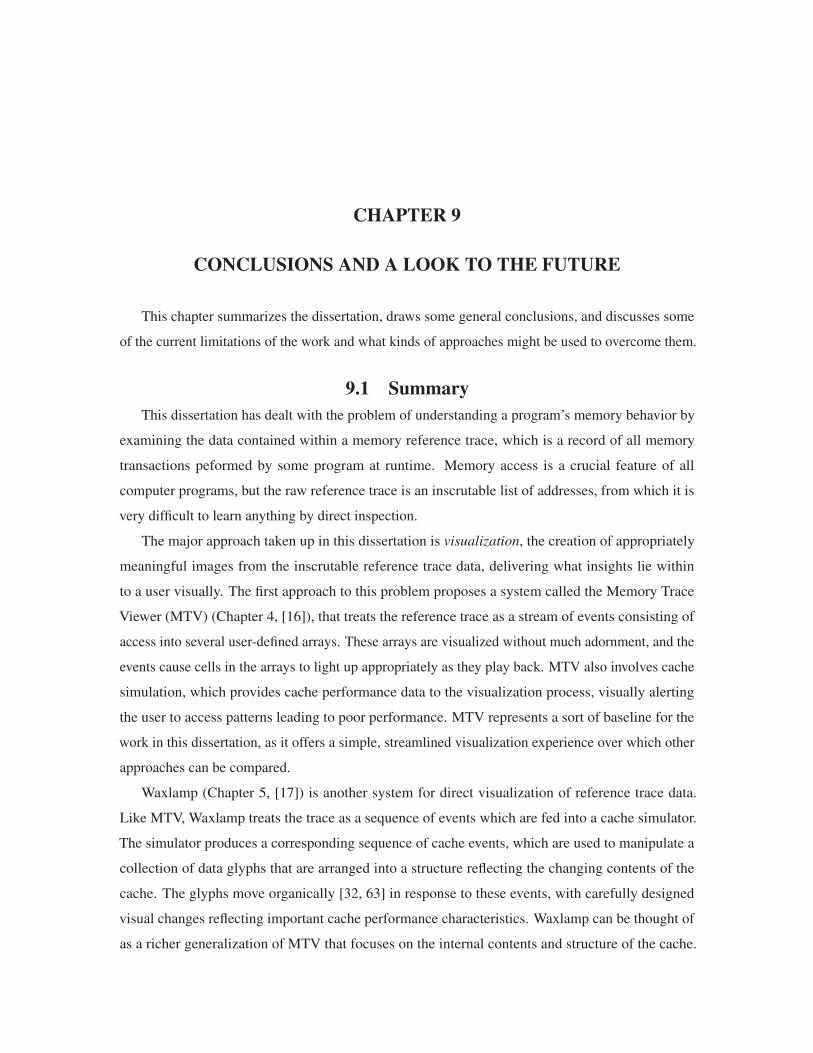
CHAPTER 9
CONCLUSIONS AND A LOOK TO THE FUTURE
This chapter summarizes the dissertation, draws some general conclusions, and discusses some
of the current limitations of the work and what kinds of approaches might be used to overcome them.
9.1 SummaryThis dissertation has dealt with the problem of understanding a program’s memory behavior by
examining the data contained within a memory reference trace, which is a record of all memory
transactions peformed by some program at runtime. Memory access is a crucial feature of all
computer programs, but the raw reference trace is an inscrutable list of addresses, from which it is
very difficult to learn anything by direct inspection.
The major approach taken up in this dissertation is visualization, the creation of appropriately
meaningful images from the inscrutable reference trace data, delivering what insights lie within
to a user visually. The first approach to this problem proposes a system called the Memory Trace
Viewer (MTV) (Chapter 4, [16]), that treats the reference trace as a stream of events consisting of
access into several user-defined arrays. These arrays are visualized without much adornment, and the
events cause cells in the arrays to light up appropriately as they play back. MTV also involves cache
simulation, which provides cache performance data to the visualization process, visually alerting
the user to access patterns leading to poor performance. MTV represents a sort of baseline for the
work in this dissertation, as it offers a simple, streamlined visualization experience over which other
approaches can be compared.
Waxlamp (Chapter 5, [17]) is another system for direct visualization of reference trace data.
Like MTV, Waxlamp treats the trace as a sequence of events which are fed into a cache simulator.
The simulator produces a corresponding sequence of cache events, which are used to manipulate a
collection of data glyphs that are arranged into a structure reflecting the changing contents of the
cache. The glyphs move organically [32, 63] in response to these events, with carefully designed
visual changes reflecting important cache performance characteristics. Waxlamp can be thought of
as a richer generalization of MTV that focuses on the internal contents and structure of the cache.

132
MTV and Waxlamp use animation in different ways to play back the events encoded in a reference
trace using various visual metaphors. These approaches allow the viewer to see what happens during
the program’s run—they are direct visualization techniques for the events encoded in the trace.
Taking a different tack, topological analysis (Chapter 6, [19]) of reference traces is concerned
with inducing a nontrivial structure on the sequence of trace records. The trivial structure of
reference traces—a linear sequence indexed by time—is very important to MTV and Waxlamp,
which essentially work by animating this sequence. However, program source code and program
runtime behavior are decidedly nonlinear, engaging in branches, loops, function calls, etc. The
topological analysis strives to find cycles in the sequence of memory accesses, which are assumed
to correspond to recurrent behavior in the program. Experiments using topological persistence to
guide the selection of computed cycles demonstrates that those cycles found in the trace with high
persistence seem to always correspond to significant runtime program structures. The cycles are
visualized using spirals, in which the radial position of the spiral encodes the passage of time—this
technique therefore visualizes the whole trace as a shape in two dimensions, giving a visualization of
the history of a program’s execution.
Finally, taking a longer perspective, visualization of cache simulation ensembles (Chapter 7)
enables the investigation of the differential behavior among several reference traces or simulations.
Ensembles are formed by running a single trace through many simulated caches, or by running
different traces through a single simulated cache, etc. This enables investigating the effect of some
difference—whether in some feature of the cache, such as size, or some feature of the program,
such as choice of algorithm—upon a program’s memory performance. Traditional information
visualization techniques are used to produce plots of a performance metric as a function of time, and
variations in performance can be seen in the deviation of the ensemble members from each other.
A sequence of case studies demonstrates the wide range of insights that can be gained from the
technique. This approach, along with the topological analysis approach, serves to visualize global
trends and structures in reference traces. They allow for viewing a longer period of time—even all
history—in a single glance.
Together, these four approaches represent a spectrum of techniques that can be used to investigate
program memory behavior. Extensions to these ideas, as well as wholly new ideas, will help to
continue this line of investigation, hopefully bringing benefit to software developers and others
interested in high performance software.
9.2 Ideas for Future WorkUnfortunately, ideas can be conceived faster than they can be prototyped and tested. However,
examination of research ideas and a discussion about their strengths and shortcomings (Chapter 8)
133
can suggest likely candidates for fruitful future work.
9.2.1 Space-for-Time Visual EncodingsMTV and Waxlamp use a time-for-time visual encoding—i.e., they use animation to display the
contents of the trace. As demonstrated by the topological and ensemble approaches, it can be very
valuable to instead use a space-for-time encoding, so that the course of history can be plotted across
a display. Some way to re-encode the trace events within MTV and Waxlamp using a space-for-time
encoding could therefore be of great value. Currently, both approaches use two-dimensional rendering
to visualize a given moment; therefore, three-dimensional visualizations might be a good way to
encode time into the third dimension. Such schemes would strive to display both the events of each
moment, and also a timeline showing many moments throughout the history of a given program run.
9.2.2 Generalized Data Structure LayoutsIn its current state, MTV hints that other data layout schemes are possible besides the simple
array layout. A two-dimensional array layout is demonstrated in Chapter 4, but many other layouts
are also possible. For instance, a layout scheme corresponding to a C-style struct or class would
allow MTV to display the data members of some instance of a class, one per row, thus using the same
abstraction that programmers use to think about such data structures. Then MTV’s visualization
abstraction could extend beyond “array item” to “class member.” This would make MTV more
flexible with respect to the kinds of data it can handle.
Similarly, Waxlamp would benefit from new schematic background structures over which to
play back traces. Chapter 5 focuses on multilevel caches for uniprocessor systems, but there are
natural generalizations of this scheme to other common memory architectures. For instance, some
systems feature multicore systems in which each core has a private L1 cache, but a shared L2 cache.
This could be visualized as a radial display in which the closest annular region around the center is
divided into two halves—one for each L1 cache. The common L2 cache would be represented as
before, with a further annular region encompassing the L1 caches and the processor at the center.
Other architectures can be modeled this way as well, depending on the meaning and behavior of their
architectural components.
9.2.3 Enabling Performance AnalysisOne of the motivations for embarking on this research program was the need for high-performance
software, and the observation that memory performance can often be a bottleneck for overall
performance. The work in this dissertation represents a first step towards using visualization to aid in
performance analysis, focusing on the primary problem of how to formulate insightful visualizations
134
for reference trace data, and identifying what these insights are. One logical next step is to move
towards the big-picture goal of performance analysis. Some results in this dissertation hint at this
goal already: for example, the analysis of row-padding in matrix multiplication (Chapter 7), and the
possibility of fusing similar functions together in a particle system (Chapter 6). However, without a
fuller execution model, from which absolute program performance could be inferred, such results
remain simply suggestions.
For example, with a full instruction trace (which, due to the inclusion of load and store
instructions, would explicitly contain a reference trace), and a method for extracting instruction-level
parallelism from it, it could be possible to formulate an execution model for a particular computing
platform, through which runtimes for some instruction stream could be estimated. Such a model
would include a performance model for the cache, with which the memory performance itself could
be estimated as some portion of the total runtime. Using this setup, the visualization approaches
in this dissertation could be extended to deal with the extra event data in a full instruction trace,
or the memory performance information could simply be used directly in the current approaches.
Essentially, generalizing from a memory reference trace to an instruction trace would open the
door to a host of new visualization techniques. Such techniques would build upon the foundation
described in this dissertation, moving concretely towards the ultimate goal of using visual analysis to
do performance analysis.
9.3 Major IssuesThe foregoing future work suggestions may end up adding value to the research ideas presented
in this dissertation. However, it is also important to acknowledge the major issues in any research, in
order to be able to meet such issues and overcome them. For the work in this dissertation, the major
limitation is scalability. This section discusses this limitation, and suggests some possible avenues of
research that might help to overcome it.
9.3.1 Data ScalabilityBy some estimates, around one third of the instructions executed by a typical program are
memory instructions [41]. With modern clock rates, even short-running programs will tend to
produce exceedingly long memory reference traces: reference traces are, therefore, generally difficult
to capture, store, and transport due to their sheer size. Pin [52] is a useful, flexible software API
for working with, among other things, a program’s reference trace records, but the naive method of
collecting a reference trace is to simply collect every trace record and store them to disk, resulting
in very dense, large data sets. However, it may be that such traces have relatively low information
content, meaning that they should be highly compressible [78]. However, the traditional approach
135
would require either collecting the trace and then compressing it afterwards using some compression
scheme, or compressing it “online” as it comes in at runtime—both approaches require an expensive
compression/decompression sequence in order to capture and use the data.
The relatively new signal processing technique called compressed sensing [26] works by taking
and storing only a very small number of measurements of an incoming signal (thereby “compressively
sensing” it); if the signal is known to be sparsely representable (i.e., compressible) in some basis,
then it can be reconstructed exactly with very high probability. It is not clear at this stage whether
compressed sensing would be a viable method of acquiring and storing reference traces. However, if
reference trace data can be demonstrated to be sparsely representable, then it should be possible to
run experiments to test the viability of compressed sensing for collecting them. The benefits of such
an approach would be a greatly reduced computational and storage burden on capturing, storing,
transporting, and even processing such traces.
9.3.2 Visualization ScalabilityWith such large traces, visualization processes are affected as well. From their sheer length,
animation methods such as MTV and Waxlamp suffer from very long playback times. This problem
could be mitigated by mining the trace for “interesting” events, producing a reduced trace of such
events, and playing these back instead of the full trace. Long traces will also cause visual clutter in
the visualization used by the topological analysis approach, as the number of records causes a large
spiral figure to be computed. Furthermore, aside from the traces being long, the simulated caches
may also be required to be very large (e.g., to approximate real-world cache configurations). This
can result in visual clutter in MTV and Waxlamp: in MTV, the cache visualization becomes too large,
while in Waxlamp, the number of data glyphs will grow until the cache levels look like solid curves
instead of a collection of independent data glyphs. Only the ensemble approach makes optimal use of
space in all cases, since it uses traditional statistical data reduction techniques to reduce the volume
of data without reducing its quality. For the other approaches, new visualization techniques, or the
integration of appropriate information visualization data volume management techniques such as
focus-and-context or level-of-detail management are needed.
9.3.3 EvaluationEvaluation is the measurement of the effectiveness of a visualization approach, according to some
quality metric. Because the purpose of visualization is to amplify human understanding, the junction
between computational image generation and human image consumption should be evaluated for the
effectiveness of information transfer or the quality of the insights induced.
A sequence of user studies could be designed to test the effectiveness of the four visualization
136
approaches presented in this dissertation. The goal would be to see how well a group of subjects
comes to understand various memory behavior scenarios using the visualization approaches, as
compared to state-of-the-art tools and basic reasoning methods. In particular, such a study could
examine the usefulness of visualization approaches for computer science education. As discussed in
Section 1.4, one of the reasons to use visualization is for explanatory or educational purposes, and a
user study with students would be able to evaluate the work in this dissertation towards those ends.
By contrast, expert reviews could be used to evaluate the techniques for the other two major
reasons for performing visualization: confirmation of hypotheses, and exploration of data. These
purposes presuppose a deeper knowledge of the visualization domain area, and therefore expert
users are the ideal target group for such a study. These could take the form of memory reference
traces with some predetermined behavioral pattern, which the experts are to investigate using the
visualization techniques, and then collecting feedback on what they are able to learn. By seeing what
kinds of hypotheses the experts form, and how they use the visualization to confirm or disconfirm
them, the usefulness of these techniques for that visualization purpose could be measured. More
generally, if the techniques were published as, e.g., a web-based toolset, then a much larger group
of people would be able to use them, leaving feedback about what kinds of tasks they are able to
perform. By exposing the visualization techniques in this way, the usefulness of the exploratory
aspect of visualization could be evaluated as well.
The work in this dissertation was evaluated via informal expert reviews, in which colleagues of
the author with varying levels of familiarity with the memory subsystem were shown prototypes
of the visualization methods, and some feedback was collected to improve the visualization design.
However, because this dissertation explores an area largely untouched by visualization methods, both
formal user studies, and formal expert reviews would provide much data on both the effectiveness of
the techniques themselves, and on the quality of the visual design comprising them. Such evaluation
studies could have a profound effect on the future directions such research would take, and therefore
are valuable to perform.
9.4 Final ThoughtsThe initial impetus for developing the work in this dissertation came from a desire to understand
the performance characteristics of a computational mechanics simulation software. As memory
peformance is often a performance bottleneck, this desire boiled down to a need to examine memory
access behavior, and somehow quantify its performance. MTV was originally born from the
observation that there was no existing visualization approach to understanding memory access
behavior. The major contribution of that system was to render something visible that formerly could
137
only be discussed in weak, abstract terms—visualization provided a mental handle for stabilizing
and strengthening reasoning efforts.
From here, the ball began rolling: other approaches to visualization, and other possibilities for
deriving insight from the traces themselves were one by one conceived, prototyped, and tested. In
each case, colleagues viewing demonstrations of the work have commented on how interesting it is
to even be able to see these concepts. Whether they help students learn about computer architecture,
or deliver performance-related insights in important code bases, the work in this dissertation has
already been shown to deliver insights about programs. Further work and play will show how far
these insights can go. The longest-term hope of working on such research ideas is that they will one
day become as commonplace and as easy to use as debuggers are today, and when that day arrives,
memory behavior will be no more mysterious to students, teachers, programmers, and developers
than any other deeply understood concept in computer science.
REFERENCES
[1] E. E. AFTANDILIAN, S. KELLEY, C. GRAMAZIO, N. RICCI, S. L. SU, AND S. Z. GUYER,
Heapviz: Interactive heap visualization for program understanding and debugging, in
Proceedings of the 5th international symposium on Software visualization, 2010, pp. 53–62.
[2] APPLE CORPORATION, Optimize with shark. http://developer.apple.com/tools/shark_optimize.html, May 2011.
[3] M. BALZER, A. NOACK, O. DEUSSEN, AND C. LEWERENTZ, Software landscapes:Visualizing the structure of large software systems, in Proceedings of the Eurographics
Symposium on Visualization (VisSym 2004), 2004, pp. 261–266.
[4] S. G. BARDENHAGEN AND E. M. KOBER, The generalized interpolation material pointmethod, Computer Modeling in Engineering and Sciences, 5 (2004), pp. 477–496.
[5] L. BASS, P. CLEMENTS, AND R. KAZMAN, Software Architecture in Practice, Addison-
Wesley Professional, 2nd ed., 2003.
[6] L. A. BELADY, A study of replacement algorithms for a virtual-storage computer, IBM Syst.
J., 5 (1966), pp. 78–101.
[7] P. BENDICH, H. EDELSBRUNNER, AND M. KERBER, Computing robustness and persistencefor images, IEEE Trans. Vis. Comput. Graph., 16 (2010), pp. 1251–1260.
[8] R. E. BRYANT AND D. R. O’HALLARON, Computer Systems: A Programmer’s Perspective,
Addison Wesley, 2nd ed., February 2010.
[9] G. CARLSSON, A. J. ZOMORODIAN, A. COLLINS, AND L. J. GUIBAS, Persistence barcodesfor shapes, Proc. Eurographs/ACM SIGGRAPH Symposium on Geometry Processing, (2004),
pp. 124–135.
[10] S. CHATTERJEE, E. PARKER, P. J. HANLON, AND A. R. LEBECK, Exact analysis of thecache behavior of nested loops, SIGPLAN Not., 36 (2001), pp. 286–297.
[11] F. CHAZAL, D. COHEN-STEINER, M. GLISSE, L. J. GUIBAS, AND S. Y. OUDOT, Proximityof persistence modules and their diagrams, Proc. 25th Ann. Sympos. Comput. Geom., (2009),
pp. 237–246.
[12] C. CHEN AND M. KERBER, Persistent homology computation with a twist, Proc. 27th
European Workshop Comput. Geom., (2011).
[13] D. CHISNALL, M. CHEN, AND C. HANSEN, Knowledge-based out-of-core algorithms fordata management in visualization, in EuroVis, 2006, pp. 107–114.
[14] , Ray-driven dynamic working set rendering, The Visual Computer, 23 (2007), pp. 167–
179.
139
[15] H.-T. CHOU AND D. J. DEWITT, An evaluation of buffer management strategies for relationaldatabase systems, in VLDB’85, Proceedings of 11th International Conference on Very Large
Data Bases, August 21-23, 1985, Stockholm, Sweden, A. Pirotte and Y. Vassiliou, eds.,
Morgan Kaufmann, 1985, pp. 127–141.
[16] A.N.M. I. CHOUDHURY, K. C. POTTER, AND S. G. PARKER, Interactive visualization formemory reference traces, Computer Graphics Forum, 27 (2008), pp. 815–822.
[17] A.N.M. I. CHOUDHURY AND P. ROSEN, Abstract visualization of runtime memory behavior,
Proc. 6th IEEE Int. Workshop on Visualizing Software for Understanding and Analysis,
(2011).
[18] A.N.M. I. CHOUDHURY, M. D. STEFFEN, J. E. GUILKEY, AND S. G. PARKER, Enhancedunderstanding of particle simulations through deformation-based visualization, Computer
Modeling in Engineering & Sciences, 63 (2010), pp. 117–136.
[19] A.N.M. I. CHOUDHURY, B. WANG, P. ROSEN, AND V. PASCUCCI, Topological analysisand visualization of cyclical behavior in memory reference traces, in Proceedings of IEEE
Pacific Visualization 2012, February 2012.
[20] T. H. CORMEN, C. E. LEISERSSON, R. L. RIVEST, AND C. STEIN, Introduction toAlgorithms, MIT Press, 2009.
[21] J. H. CROSS, II, T. D. HENDRIX, AND S. MAGHSOODLOO, The control structure diagram:An overview and initialevaluation, Empirical Software Engineering, 3 (1998), pp. 131–158.
[22] V. DE SILVA AND G. CARLSSON, Topological estimation using witness complexes, Symp. on
Point-Based Graph., (2004), pp. 157–166.
[23] V. DE SILVA, D. MOROZOV, AND M. VEJDEMO-JOHANSSON, Persistent cohomology andcircular coordinates, Proc. 25th Ann. Sympos. Comput. Geom., (2009), pp. 227–236.
[24] , Dualities in persistent (co)homology. Manuscript, 2010.
[25] S. DIEHL, Software Visualization: Visualizing the Structure, Behaviour, and Evolution ofSoftware, Springer, 2007.
[26] D. L. DONOHO, Compressed sensing, IEEE Transactions on Information Theory, 52 (2006),
pp. 1289–1306.
[27] H. EDELSBRUNNER, D. LETSCHER, AND A. J. ZOMORODIAN, Topological persistence andsimplification, Discrete Comput. Geom., 28 (2002), pp. 511–533.
[28] J. EDLER AND M. D. HILL, Dinero IV trace-driven uniprocessor cache simulator. http://www.cs.wisc.edu/˜markhill/DineroIV.
[29] M. EIGLSPERGER, C. GUTWENGER, M. KAUFMANN, J. KUPKE, M. JUNGER, S. LEIPERT,
K. KLEIN, P. MUTZEL, AND M. SIEBENHALLER, Automatic layout of uml class diagrams inorthogonal style, Information Visualization, 3 (2004), pp. 189–208.
[30] A. A. EVSTIOUGOV-BABAEV, Call graph and control flow graph visualization for developersof embedded applications, in Revised Lectures on Software Visualization, International
Seminar, London, UK, UK, 2002, Springer-Verlag, pp. 337–346.
[31] M. FOWLER, UML Distilled: A Brief Guide to the Standard Object Modeling Language,
Addison-Wesley Professional, 3rd ed., 2003.

140
[32] B. J. FRY, Organic information design, Master’s thesis, Massachusetts Institute of Technology,
May 2000.
[33] GNU FOUNDATION, GNU gprof. ftp://ftp.gnu.org/old-gnu/Manuals/gprof-2.9.1/gprof.html,
March 2012.
[34] GNU PROJECT, Ddd—data display debugger. http://www.gnu.org/software/ddd/, March 2012.
[35] , Gcc, the gnu compiler collection. http://gcc.gnu.org, March 2012.
[36] H. H. GOLDSTINE AND J. VON NEUMANN, Planning and coding of problems for anelectronic computing instrument, tech. rep., Institute for Advanced Study, Princeton, NJ,
1948.
[37] K. GRIMSRUD, J. ARCHIBALD, R. FROST, AND B. NELSON, Locality as a visualizationtool, IEEE Transactions on Computers, 45 (1996), pp. 1319–1326.
[38] J. GRUNDY AND J. HOSKING, Softarch: Tool support for integrated software architecturedevelopment, International Journal of Software Engineering and Knowledge Engineering, 13
(2003), pp. 125–152.
[39] C. D. HANSEN AND C. R. JOHNSON, eds., The Visualization Handbook, Academic Press,
1st ed., December 2004.
[40] A. HATCHER, Algebraic Topology, Cambridge University Press, 2002.
[41] J. L. HENNESSY AND D. A. PATTERSON, Computer Architecture: A Quantitative Approach,
Morgan Kaufmann Publishers, 3rd ed., 2003.
[42] M. HILL AND A. SMITH, Evaluating associativity in cpu caches, Computers, IEEE Transac-
tions on, 38 (1989), pp. 1612 –1630.
[43] INTEL CORPORATION, Intel VTune amplifier XE 2011. http://software.intel.com/sites/products/documentation/hpc/amplifierxe/en-us/lin/start/index.htm, May 2011.
[44] M. ISENBURG AND S. GUMHOLD, Out-of-core compression for gigantic polygon meshes,
ACM Trans. Graph., 22 (2003), pp. 935–942.
[45] M. A. JACKSON, Principles of Program Design, Academic Press, 1975.
[46] S. F. KAPLAN, Y. SMARAGDAKIS, AND P. R. WILSON, Flexible reference trace reductionfor VM simulations, ACM Trans. Model. Comput. Simul., 13 (2003), pp. 1–38.
[47] K. KENNEDY AND K. MCKINLEY, Maximizing loop parallelism and improving data localityvia loop fusion and distribution, Proc. 6th Int. Workshop on Lang. and Compilers for Par.
Comp., (1994), pp. 301–320.
[48] D. J. KERBYSON, A. H. J., A. HOISIE, F. PETRINI, H. J. WASSERMAN, AND M. GITTINGS,
Predictive performance and scalability modeling of a large-scale application, in Proceedings
of the 2001 ACM/IEEE conference on Supercomputing (CDROM), Supercomputing ’01, New
York, NY, USA, 2001, ACM, pp. 37–37.

141
[49] C. KNIGHT AND M. MUNRO, Comprehension with[in] virtual environment visualisations,
in Proceedings of the 7th International Workshop on Program Comprehension, IWPC ’99,
Washington, DC, USA, 1999, IEEE Computer Society, pp. 4–.
[50] D. E. KNUTH, Structured programming with go to statements, Computing Surveys, 6 (1974),
pp. 261–301.
[51] H. KONING, C. DORMANN, AND H. VAN VLIET, Practical guidelines for the readabilityof it-architecture diagrams, in Proceedings of the 20th Annual International Conference on
Documentation, ACM SIGDOC 2002, 2002, pp. 90–99.
[52] C.-K. LUK, R. COHN, R. MUTH, H. PATIL, A. KLAUSER, G. LOWNEY, S. WALLACE,
V. J. REDDI, AND K. HAZELWOOD, Pin: building customized program analysis tools withdynamic instrumentation, in PLDI, 2005, pp. 190–200.
[53] J. MALONEY, M. RESNICK, N. RUSK, B. SILVERMAN, AND E. EASTMOND, The scratchprogramming language and environment, Transactions on Computing Education, 10 (2010),
pp. 16:1–16:15.
[54] D. R. MARTIN, Sorting algorithm animations. http://www.sorting-algorithms.com, March 2012.
[55] E. MASCIARI, C. PIZZUTI, G. RAIMONDO, AND D. TALIA, Using an out-of-core techniquefor clustering large data sets, in Database and Expert Systems Applications, 2001. Proceedings.
12th International Workshop on, 2001, pp. 133–137.
[56] J. R. MUNKRES, Elements of algebraic topology, Addison-Wesley, Redwood City, CA, USA,
1984.
[57] G. MURPHY, M. KERSTEN, AND L. FINDLATER, How are java software developers usingthe elipse ide?, Software, IEEE, 23 (2006), pp. 76–83.
[58] W. E. NAGEL, A. ARNOLD, M. WEBER, H.-C. HOPPE, AND K. SOLCHENBACH, VAMPIR:Visualization and analysis of MPI resources, Supercomputer, 12 (1996), pp. 69–80.
[59] I. NASSI AND B. SHNEIDERMAN, Flowchart techniques for structured programming,
SIGPLAN Notices, 8 (1973), pp. 12–26.
[60] NATIONAL INSTRUMENTS, NI labVIEW—improving the productivity of engineers andscientists. http://www.ni.com/labview/, March 2012.
[61] N. NETHERCOTE, Dynamic Binary Analysis and Instrumentation, PhD thesis, University of
Cambridge, November 2004.
[62] F. NIELSON, H. R. NIELSON, AND C. HANKIN, Principles of Program Analysis, Springer,
corrected ed., 2004.
[63] M. OGAWA AND K.-L. MA, code swarm: A design study in organic software visualization,
IEEE Transactions on Visualization and Computer Graphics, 15 (2009), pp. 1097–1104.
[64] T. PANAS, R. BERRIGAN, AND J. GRUNDY, A 3d metaphor for software productionvisualization, in Proceedings of the 7th International Conference on Information Visualization,
2003, pp. 314–319.
[65] A. T. PANG, C. M. WITTENBRINK, AND S. K. LODH, Approaches to uncertainty visualiza-tion, The Visual Computer, 13 (1996), pp. 370–390.
142
[66] C. Y. PARK, Predicting program execution times by analyzing static and dynamic programpaths, Real-Time Syst., 5 (1993), pp. 31–62.
[67] S. PARKER, P. SHIRLEY, Y. LIVNAT, C. HANSEN, AND P.-P. SLOAN, Interactive ray tracingfor isosurface rendering, in Visualization 1998 Proceedings, October 1998, pp. 233–238.
[68] S. G. PARKER AND C. R. JOHNSON, Scirun: A scientific programming environment forcomputational steering, in Proceedings of the 1995 ACM/IEEE conference on Supercomputing
(CDROM), Supercomputing ’95, New York, NY, USA, 1995, ACM.
[69] K. POTTER, J. KNISS, R. RIESENFELD, AND C. JOHNSON, Visualizing summary statisticsand uncertainty, Computer Graphics Forum, 29 (2010), pp. 823–832.
[70] K. POTTER, A. WILSON, P.-T. BREMER, D. WILLIAMS, C. DOUTRIAUX, V. PASCUCCI,
AND C. JOHNSON, Ensemble-vis: A framework for the statistical visualization of ensembledata, in Data Mining Workshops, 2009. ICDMW ’09. IEEE International Conference on, dec.
2009, pp. 233 –240.
[71] H. PROKOP, Cache-oblivious algorithms, Master’s thesis, Massachusetts Institute of Technol-
ogy, June 1999.
[72] B. QUAING, J. TAO, AND W. KARL, Yaco: A user conducted visualization tool for supportingcache optimization, in Proceedings of HPCC, 2005, pp. 694–703.
[73] D. QUINLAN, ROSE: Compiler support for object-oriented frameworks, Parallel Processing
Letters, 10 (2000), pp. 215–226.
[74] S. P. REISS, Visualizing java in action, in SoftVis ’03: Proceedings of the 2003 ACM
symposium on Software visualization, New York, NY, USA, 2003, ACM, pp. 57–ff.
[75] S. P. REISS AND M. RENIERIS, Jove: Java as it happens, in SoftVis ’05: Proceedings of
the 2005 ACM symposium on Software visualization, New York, NY, USA, 2005, ACM,
pp. 115–124.
[76] J. SANYAL, S. ZHANG, J. DYER, A. MERCER, P. AMBURN, AND R. MOORHEAD, Noodles:A tool for visualization of numerical weather model ensemble uncertainty, IEEE Transactions
on Visualization and Computer Graphics, 16 (2010), pp. 1421–1430.
[77] R. SCHALLER, Moore’s law: Past, present and future, Spectrum, IEEE, 34 (1997), pp. 52
–59.
[78] C. E. SHANNON, A mathematical theory of communication, Bell System Technical Journal,
27 (1948), pp. 379–423.
[79] S. S. SHENDE AND A. D. MALONY, The TAU parallel performance system, International
Journal of High Performance Computing Applications, 20 (2006), pp. 287–331.
[80] A. J. SMITH, Two methods for the efficient analysis of memory address trace data, IEEE
Trans. Softw. Eng., 3 (1977), pp. 94–101.
[81] J. STASKO, Animating algorithms with xtango, ACM SIGACT News, 23 (1992), pp. 67–71.
[82] J. T. STASKO, Tango: A framework and system for algorithm animation, Computer, 23 (1990),
pp. 27–39.
143
[83] F. STEINBRUCKNER AND C. LEWERENTZ, Representing development history in softwarecities, in Proceedings of the 5th international symposium on Software visualization, SOFTVIS
’10, New York, NY, USA, 2010, ACM, pp. 193–202.
[84] C. STOLTE, R. BOSCH, P. HANRAHAN, AND M. ROSENBLUM, Visualizing applicationbehavior on superscalar processors, in Information Visualization, 1999, pp. 10–17.
[85] D. SULSKY, Z. CHEN, AND H. SCHREYER, A particle method for history-dependentmaterials, Computer Methods in Applied Mechanics and Engineering, 118 (1994), pp. 179 –
196.
[86] D. SULSKY, S.-J. ZHOU, AND H. L. SCHREYER, Application of a particle-in-cell method tosolid mechanics, Comput. Phys. Comm., 87 (1995), pp. 236–252.
[87] D. TARJAN, S. THOZIYOOR, AND N. P. JOUPPI, CACTI 4.0, Tech. Rep. HPL-2006-86, HP
Laboratories, Palo Alto, June 2006.
[88] J. B. TENENBAUM, V. DE SILVA, AND J. C. LANGFORD, A global geometric framework fornonlinear dimensionality reduction, Science, 290 (2000), pp. 2319–2323.
[89] D. TERPSTRA, H. JAGODE, H. YOU., AND J. DONGARRA, Collecting performance datawith PAPI-C, in Tools for High Performance Computing, 2009, pp. 157–173.
[90] S. TOLEDO, External memory algorithms, American Mathematical Society, Boston, MA,
USA, 1999, ch. A survey of out-of-core algorithms in numerical linear algebra, pp. 161–179.
[91] A. M. TURING, On computable numbers, with an application to the entscheidungsproblem,
Proceedings of the London Mathematical Society, 2 (1937), pp. 230–265.
[92] R. A. UHLIG AND T. N. MUDGE, Trace-driven memory simulation: A survey, ACM
Computing Surveys, 29 (1997), pp. 128–170.
[93] E. VAN DER DEIJL, G. KANBIER, O. TEMAM, AND E. GRANSTON, A cache visualizationtool, Computer, 30 (1997), pp. 71–78.
[94] J. WALNY, J. HABER, M. DORK, J. SILLITO, AND S. CARPENDALE, Follow that sketch:Lifecycles of diagrams and sketches in software development, in 6th IEEE International
Workshop on Visualizing Software for Understanding and Analysis (VISSOFT 2011), 2011.
[95] B. WANG, B. SUMMA, V. PASCUCCI, AND M. VEJDEMO-JOHANSSON, Branching andcircular features in high dimensional data, IEEE Trans. Vis. Comput. Graph., 17 (2011),
pp. 1902–1911.
[96] J. WEIDENDORFER, M. KOWARSCHIK, AND C. TRINITIS, A tool suite for simulation basedanalysis of memory access behavior, in Computational Science - ICCS 2004, M. Bubak,
G. van Albada, P. Sloot, and J. Dongarra, eds., vol. 3038 of Lecture Notes in Computer
Science, Springer Berlin / Heidelberg, 2004, pp. 440–447.
[97] W. A. WULF AND S. A. MCKEE, Hitting the memory wall: Implications of the obvious,
Computer Architecture News, 23 (1995), pp. 20–24.
[98] S.-E. YOON, P. LINDSTROM, V. PASCUCCI, AND D. MANOCHA, Cache-oblivious meshlayouts, ACM Trans. Graph., 24 (2005), pp. 886–893.
[99] Y. YU, K. BEYLS, AND E. D’HOLLANDER, Visualizing the impact of the cache on programexecution, in Information Visualization, 2001, pp. 336–341.

144
[100] Y. ZHONG, M. ORLOVICH, X. SHEN, AND C. DING, Array regrouping and structuresplitting using whole-program reference affinity, in Proceedings of the ACM SIGPLAN 2004
Conference on Programming Language Design and Implementation, 2004, pp. 255–266.
[101] Y. ZHONG, X. SHEN, AND C. DING, A hierarchical model of reference affinity, Proc. 16th
Int. Workshop on Lang. and Compilers for Par. Comp., (2003).
[102] A. J. ZOMORODIAN, Fast construction of the Vietoris-Rips complex, Comput. Graph., 34
(2010), pp. 263–271.