Mathematical models of shape memory alloy behavior for online and fast prediction of the hysteretic behavior

H. Shibly*•, D. Söffker•

*Mechanical Engineering Department, Faculty of Engineering, Birzeit University,

Birzeit, Palestine •Chair of Dynamics and Control, Faculty of Engineering Sciences, University of Duisburg-Essen,

D-47048 Duisburg, Germany

In this contribution a new closed form of a mathematical model of Nickel-Titanium (NiTi) shape memory alloy (SMA) and its thermo-mechanical wire hysteresis behavior is developed. The approach is based on experimental data. The behavior of the heated and naturally cooled wire is modeled by mathematical expression. The cycle of heating and cooling is performed under a constant load. The prediction of the hysteretic behavior is realized through models adaptation, as predetermination, or real time determination of the models values, is developed and presented in detail. Simulations for position control using PID controller is shown for comparison purposes. The developed approach is incorporated in a feed forward control scheme. A comparison between the actual position and the predicted models position shows promising results.

Keywords: SMA hysteric behavior, prediction, modeling, and simulation. 1. Introduction

The materials behavior of Shape Memory Alloy (SMA) is within the focus and the attention of researchers and engineers on its peculiar characteristics for its potential of wide range of use: as micro actuators, vascular stents, guide wires, catheters, orthodontic appliances, eyeglass frames, cellular phone antennas, valves, fasteners, and heating of thermostats. Beside the practical use of the material, another interesting use is controlling the force and the geometrical properties of the material to effect the shape of the rotor blades of helicopter, to improve lift and reduction of vibrations [1, 2] etc. SMA wires, such as Nickel-Titanium (Ni-Ti) wires, have a peculiar property of contracting in its length upon heating and expanding upon cooling [3]; as a result, the material can be used as actuator realizing forces or changing positions. This behavior is called in literature the Shape Memory Effect (SME). The SME occurs when the material undergoes a phase change, for example by heating above a certain transition temperature or vice versa by cooling. The modeling of the SMA-material behavior is within the focus of current research, c. f. [4, 5, and 6]. The observed complex hysteretic behavior is typically modeled by physical-oriented complex models, able to describe the physics of the system (especially the phase changes) on an elementary level. The focus of the actual and typical related model development is the representation of the hysteretic effects by implementing internal memory using Preissach operators [7, 8] or other suitable approaches. The validation of the models shows that the material behavior can be expressed and mathematically expressed. The disadvantage of such kind of models is that due to their complex implicit representation, they can not be used for online- or real time purposes. This aspect mainly results from necessary spatial integrations during time-integration. The main idea of this contribution is to express explicit models modeling the phenomenological material behavior for online use, resp. to be used as model for model-based SMA-force or position control. Therefore of course some assumptions have to be made, discussed in the sequel.

* Corresponding author. Email address: hshibli@birzeit.edu The paper is organized as follows: in Chapter 2 the theoretical and motivational background is briefly illustrated; Chapter 3 explains the mathematical modeling approach in detail. The experimental results are illustrated, compared with simulated results, in Chapter 4. In Chapter 5 a very short and initial control approach is implemented, whereby in Chapter 6 a conclusion and final remarks are given. 2. Theoretical background The effects of the shape memory effect (SME) and pseudo elasticity of SMA are described schematically in Figure 1. Starting with Austenite as phase-A, cooling down under the martensite finish transition temperature Mf , a twinned martensite is achieved, denoted as phase-B, or by external loading a detwinned martensite is achieved, denoted as phase-C. The pairs of martensite twins begin ‘detwinning’ to the stress-preferred variant as phase-C. Heating up the detwinned martensite phase above the austenite phase transition temperature Af the transformation to austenite phase occurs again and recovers its original geometric configuration. This behavior is called SME. The process and the physical background is given in detail in [9, 10, and 11].

Figure 1. Schematic description of shape memory effect and pseudo elasticity that are caused by detwinning and phase transformation among ((A) austenite, (B) twinned martensite, (C) detwinned martensite).

Similarly applying load, austenite phase transforms to stress-induced martensite, as phase-C. But when de-twinned martensite as phase-C is unloaded, it transforms to austenite; which is called pseudo-elasticity [12]. The difference between the transition temperatures upon heating and cooling of shape memory alloy results to hysteretic behavior as shown in Figure 2.

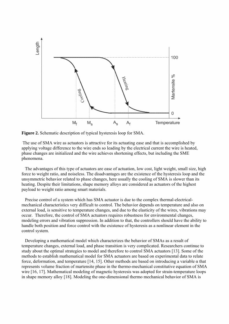
Figure 2. Schematic description of typical hysteresis loop for SMA.

The use of SMA wire as actuators is attractive for its actuating ease and that is accomplished by applying voltage difference to the wire ends so leading by the electrical current the wire is heated, phase changes are initialized and the wire achieves shortening effects, but including the SME phenomena. The advantages of this type of actuators are ease of actuation, low cost, light weight, small size, high force to weight ratio, and noiseless. The disadvantages are the existence of the hysteresis loop and the unsymmetric behavior related to phase changes, here usually the cooling of SMA is slower than its heating. Despite their limitations, shape memory alloys are considered as actuators of the highest payload to weight ratio among smart materials. Precise control of a system which has SMA actuator is due to the complex thermal-electrical-mechanical characteristics very difficult to control. The behavior depends on temperature and also on external load, is sensitive to temperature changes, and due to the elasticity of the wires, vibrations may occur. Therefore, the control of SMA actuators requires robustness for environmental changes, modeling errors and vibration suppression. In addition to that, the controllers should have the ability to handle both position and force control with the existence of hysteresis as a nonlinear element in the control system. Developing a mathematical model which characterizes the behavior of SMAs as a result of temperature changes, external load, and phase transition is very complicated. Researchers continue to study about the optimal strategies to model and therefore to control SMA actuators [13]. Some of the methods to establish mathematical model for SMA actuators are based on experimental data to relate force, deformation, and temperature [14, 15]. Other methods are based on introducing a variable α that represents volume fraction of martensite phase in the thermo-mechanical constitutive equation of SMA wire [16, 17]. Mathematical modeling of magnetic hysteresis was adopted for strain-temperature loops in shape memory alloy [18]. Modeling the one-dimensional thermo mechanical behavior of SMA is

divided into four categories [19] where the constitutive models [12, 20-22] are focused on describing different aspects of SMA. The scope of this contribution is different: instead of theoretical modeling representing also the internal physical effects, here a phenomenological approach is realized. The idea is to use mathematical modeling; this includes that the developed models should represent the same Input-Output behavior as observed in experiments, based on a simplified and perfectly explicit closed mathematical expressions. They will build the base for further and easier realization of model-based control approaches. 3. Model development

Typical experimental data that relates length change of SMA to temperature change during heating and cooling [23] are shown in Figure 3 showing a hysteresis loop with two sides. The upper side is for heating while the lower side is for ‘free’ cooling. The two curves diverge at low temperature (T1, Y1) and converge back at high temperature (T2, Y2). The two points are denoted the first and second common points respectively. In order to explain the model development a schematic drawing of an experimental hysteresis loop is shown in Figure 4.

Figure 3. Hysteresis loop of experimental results of NiTi SMA loaded wire [20].

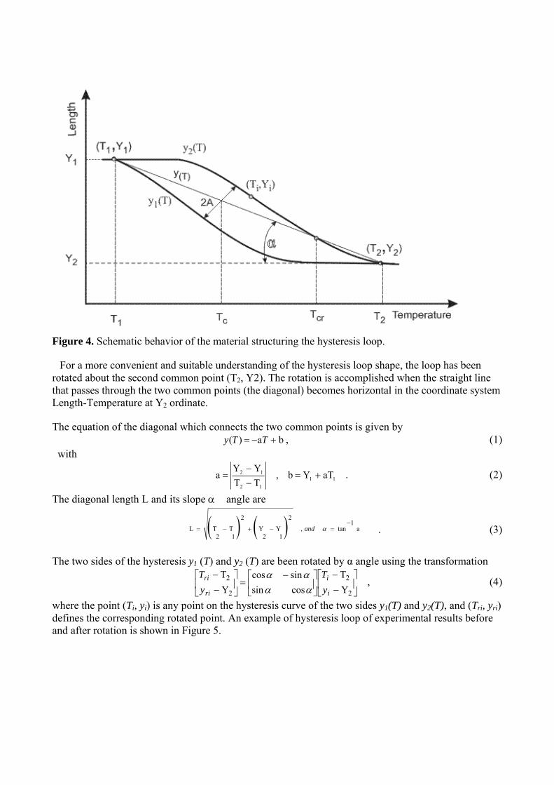
Figure 4. Schematic behavior of the material structuring the hysteresis loop.

For a more convenient and suitable understanding of the hysteresis loop shape, the loop has been rotated about the second common point (T2, Y2). The rotation is accomplished when the straight line that passes through the two common points (the diagonal) becomes horizontal in the coordinate system Length-Temperature at Y2 ordinate. The equation of the diagonal which connects the two common points is given by

ba)( TTy , (1) with

11

12

12 aTYb,TT

YYa

. (2)

The diagonal length L and its slope �angle are

2 21

L T T Y Y , tan a2 1 2 1

and

. (3)

The two sides of the hysteresis y1 (T) and y2 (T) are been rotated by α angle using the transformation

2

2

2

2

Y

T

cossin

sincos

Y

T

i

i

ri

ri

y

T

y

T

, (4)

where the point (Ti, yi) is any point on the hysteresis curve of the two sides y1(T) and y2(T), and (Tri, yri) defines the corresponding rotated point. An example of hysteresis loop of experimental results before and after rotation is shown in Figure 5.

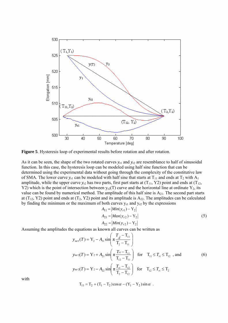
Figure 5. Hysteresis loop of experimental results before rotation and after rotation.

As it can be seen, the shape of the two rotated curves yr1 and yr2 are resemblance to half of sinusoidal function. In this case, the hysteresis loop can be modeled using half sine function that can be determined using the experimental data without going through the complexity of the constitutive law of SMA. The lower curve yr1 can be modeled with half sine that starts at T11 and ends at T2 with A1 amplitude, while the upper curve yr2 has two parts, first part starts at (T11, Y2) point and ends at (T12, Y2) which is the point of intersection between yr2(T) curve and the horizontal line at ordinate Y2, its value can be found by numerical method. The amplitude of this half sine is A21. The second part starts at (T12, Y2) point and ends at (T2, Y2) point and its amplitude is A22. The amplitudes can be calculated by finding the minimum or the maximum of both curves yr1 and yr2 by the expressions

2222

2221

2111

Y)(

Y)(

Y)(

r

r

r

yMinA

yMaxA

yMinA

(5)

Assuming the amplitudes the equations as known all curves can be written as

212122

122222

12111112

112122

112

11

1121

TTforTT

TπsinY)(

TTforTT

TπsinY)(

TT

TπsinY)(

riri

mr

ri

rimr

rmr

TT

ATy

TT

ATy

iT

ATy

, and (6)

with sin)YY(cos)TT(TT 2121211 .

(7) A comparison between the experimental hysteresis loop of Figure 5 and its model hysteresis loop of half sinusoidal is shown in Figure 6. In this figure, the ordinate is been enlarged to see the deviations. It shows that the two loops are almost identical.

Figure 6. Comparison between hysteresis of experimental results (blue color) and the hysteresis of the proposed mathematical model (red color) at the rotated position.

Next, the model hysteresis loop is rotated in opposite direction by the same α angle to the position of the experimental hysteresis loop using the transformation

2

2

2

2

Y

T

cossin

sincos

Y

T

mri

ri

mi

mi

yy

TT

(8)

Figure 7. Hysteresis loop of experimental results (in blue color), and hysteresis loop of mathematical model (in red color) before and after rotation. The result is shown in Figure 7. Algebraic simplification yields to a first mathematical model as :

sin)()( 321 aTyaTaaTy om , (9)

with

112

11

12

121

32

2

122

2

,TT

YYtan

,cos,sin

,cossin,cossinTcosY

TT

TT

Aaa

aa

ri

ij

o

, and (10)

All the model coefficients are based on the coordinates of the two common points (T1, Y1) and (T2, Y2). Since the previous approach is based on half sine function and curve rotation, a second mathematical model could be achieved without curve rotation which is a half sine function added to the diagonal straight line function y(T). As result, a second mathematical model appears as

sinijAaTb(T)my (11)

with

2

TTTT,cosLL

)(,cos

2

)T()T(

121c1

1

112

L

TTyyA cc

, and (12)

The positive and negative signs are for upper and lower curves respectively. The lower curve of the hysteresis loop is modeled as

21111 ,L/)T(πsina-b)( TTTTATTmy . (13) The diagonal intersects the upper curve of the hysteresis loop to two parts; one part is above the diagonal and a second part is under the diagonal. The two parts have different amplitude and length; therefore, two halves of sinusoidal functions are needed to model the upper side of the hysteresis loop. The crossing point location defines the f ratio. The two parts of the upper curve are

crm TTTTATTy 12112 ,L/)T(πsina-b)( and

22212 ,L/)T(πsina-b)( TTTTATTy crm , (14)

with 122121 L)1(L,L L ff .

To improve the model accuracy, tuning coefficients c11, c21, and c22 have been added to the model. The final form of the second mathematical model of the hysteresis loop results to

2111111 ,L/)T(πsina-b)( TTTTAcTTmy , crm TTTTAT(T)y 1211212 ,L/)T(πsincab , and

2221222 ,L/)T(πsinca-b TTTTAT(T)y crm . (15) The second mathematical model also is based on defining the two common points (T1, Y1) and (T2, Y2) of the hysteresis loop. The model steps are: defining the abscissa Tcr (the intersection point of the upper curve with the diagonal) and calculating the f ratio, estimating the abscissa Tc and the amplitude A. By knowing all the aforementioned parameters the model can be determined. Then, a calculation of the average of relative deviation is needed to check model accuracy. For unsatisfied accuracy, a fine tuning has to be done. The tuning can be achieved by moving the common points a very small distance and modifying the values of the coefficients c1, c21, and c22. A typical result is shown in Figure 8.

Figure 8. Experimentally measured hysteresis loop (a) Hysteresis loop of experimental results (blue color), and the diagonal between the common two points (black color). (b) The same as in (a), and the second mathematical model (red color). (c) The same as in (b) with tuned amplitudes. (d) The same as in (d) added to it metal expansion curve.

For higher temperature above T2, the region to the right of the hysteresis loop can be considered as a metal expansion of the SMA wire. This range can be modeled with a second order polynomial, where by its coefficients are related to the metal heat expansion properties; see Figure 8(d). Both mathematical models can be achieved based on the experimental hysteresis loop that relates the length of the SMA wire and temperature. The temperature is being determined by knowing the input electrical current and solving the following SMA wire unidirectional heat transfer equation for electrical heating and free convection by

RITThAdt

dTmc roomp

2)( , (16)

where m represents the wire mass, Cp represents specific heat, h is heat convection coefficient, A denotes the circumferential area, Troom represents the room temperature, I represents the electrical current, and R denotes the wire electrical resistance.

4. Experimental test bed

The experimental test bed at the laboratory of the Chair of Dynamics and Control, at University of Duisburg-Essen was used to perform the required tests. The test bed has besides suitable measuring devices, the capability of position and force control for SMA wire. The tests were performed on a Nitinol SMA wire of 525 mm length and 0.19 mm radius, which is connected to force sensor in one end and to a small slider at the other end. As shown in Figure 9, the slider is connected to a load through a pulley. The displacement of the slider is measured online by laser sensor. The wire was heated by electrical current that can be controlled with a DSP-system using a real time control system in combination with MATLAB and SIMULINK. The room temperature is measured by temperature sensor that is shown in Figure 10. The material properties of the SMA wire are taken from the manufacture data.

Figure 9. Schematic drawing of the test bed at Chair of Dynamics and Control, University of Duisburg-Essen.

Figure 10. Picture of the experimental test bed (Chair of Dynamics and Control at U DuE).

5. Simulations results and experimental validation

Experiments were performed for various current inputs. Therefore currents up to two amperes, in combination with constant loads of 1, 2, 3, and 4 kg are applied to the system. The results are shown in Figures 5, 6, 7, and 8. The observed behavior represents

i) the experimental hysteresis loops, whereby the diagonal connects the two common points, and ii) the mathematical model hysteresis loop.

For both models, the average of relative deviation was calculated. In the first model, the average of relative deviation was about 1.0%, illustrated in Figure 7. In the second model, the average of relative deviation was around 3%; see Figure 8(b). With amplitude modification (achieved by measuring the amplitude from the experimental data) the value of the coefficients achieved were c1=1.2, c21=1.0, and c22= 0.333. In this case, the average of relative deviation can be reduced to 1.1%; see Figure 8(c). Hysteresis loops shape change was examined for i) different preloading, ii) parameters changes, and iii) various types of excitations. With respect to i) the SMA wire was preloaded by 1, 2, 3, and 4 kg. The load remains constant during operation. The hysteresis loop change was a position shift of the loop toward up because of wire pre-elongation which is expected, also the loop gets narrower with larger load; see Figure 11(a). With respect to ii) several values of h, the coefficient of heat convection are considered and as result it can be stated that the hysteresis loop gets wider for larger value of h, while keeping the same shape of the upper side of the hysteresis loop and bending to the left the lower side of the hysteresis loop, see Figure 11(b). Similar examination was done for Cp , the specific heat coefficient, the hysteresis loop gets thinner while keeping the same shape, see Figure11(c). With respect to iii) various repeated excitations are applied: 1) The slider was given enough time to return back to its original position by letting the cooling process to be completed, the hysteresis loop repeats itself almost the same, see Figure 12(a). 2) Repeated excitations but the system was excited again before the slider reaches its original position, the result was a shift down of the upper curve of the hysteresis loop, see Figure 12(b). 3) Repeated excitations where applied so that the time between excitations is shorter than before in order to keep the slider close to its final position, in this case inner loops where achieved, see Figure 12(c).

(a)

(b)

(c)

(d)

Figure11. Hysteresis loop shape changes caused by: (a) Using four preloads. (b) Using three values of coefficient of heat convection, arrow shows larger values. (c) Using three values of specific heat convection. (d) The outer hysteresis loop of (b) and the adapted model (red color).

Model Adaption The experience, which has been achieved regarding shape changes of the hysteresis loop under different operation conditions, provides the ability to adapt the models to the new conditions. Models generalization and adaptation can be done in two ways: First, is predetermination of the two common points (T1, Y1), (T2, Y2) and amplitudes. This strategy is applicable, when the operation repeats itself under the same condition as it shown in Figure 12(a). The second strategy is a real time determination of one of the two common points and the amplitude. This way is used when the hysteresis loop changes shape. It is explained using the aforementioned tests results. As examples; 1) The third hysteresis loop in Figure 11(b) has relatively the worst shape; it's lower side bends to the left and extends its straight right part. Therefore, the model lower side is the one which has to be modified. The modification is done by taking another second common point for it, so that T2 is different from the one of the upper side. Therefore, its second common point will be to the left from its original location. In this case T2 is the only modified value and it is taken as the temperature when the change in the actual elongation becomes larger than a specific value. The adapted model is shown in Figure 11(d) in red color. 2) For repeated excitation, as in Figure 12(a), the same model can be applicable for all the hysteresis loops. In Figure 12(b) the modification is only for the first common point (T1, Y1) where the abscissa and ordinate are taken as the last values when the curve changes direction. For inner loops, as in Figure12(c), the two common points are modified as illustrated in Figure 11(d) and as in Figure 12(b). The amplitude can be modified by minimizing the deviation between the model and the measured elongation based on the first measuring values.

(a)

(b)

( c)

Figure 12. Hysteresis loops (blue color) and the adapted model (red color) for repeated excitation: (a) Complete cycle of operations. (b) Incomplete cycles of operations. (c) Short cycles within the complete one produces the inner loops.

To examine the behavior of the proposed models to be used in control systems, a SIMULINK simulation is realized for position control using standard PID controller with two different inputs, as illustrated in Figure 13. For a step input, the result is shown in Figure 14(a). The model position and the desired position are very close except at the time where cooling takes place. Since the cooling of the SMA wire is realized by a free convection process, its expansion is slower than it can be realized by the abrupt change of the step function-like heating. For a cyclic sine function input, the result is shown in Figure 14(b). In this case, a better matching along the hysteresis loop between the model position and the desired position as a result of gradual change in sine function.

Figure 13. Block diagram of SIMULINK control system.

(a) Step response function

(b) Cyclic sine input given as input produces output behavior

Figure 14. Comparison between desired position (blue color) and model position (red color), (a) for step input, (b) for cyclic sine input.

Another comparison between the experimental actual position of the SMA wire control system and the position of the model for the same current input on real time control is illustrated in the block diagram shown in Figure 15. The control system of the SMA wire, specified in section 4, uses in this case a standard PID controller. The hysteresis model block is the developed model, the heat transfer model block is developed in equation (16). The mechanical system block is the system shown in Figure 9. As an example of the comparison, results are shown in Figure 16. The major deviation between the two curves exists outside the region of the hysteresis loop which shows that the developed approach is able to realize the Input/Output behavior of complex hysteretic structures without using complex modeling approach, and has a promising use in control.

Figure 15. Block diagram of the control system.

Figure 16 . Comparison between the actual position (blue color) and the model position (red color) on real time control.

6. Conclusions In this paper two mathematical models for SMA wire behavior are developed, proposed, and validated. The closed mathematical form composed of algebraic and trigonometric functions will allow the online-use of the model. From a computational point of view, as advantage the easy implementation and realization aspects are important. The models’ parameters depend only on the coordinates of two common points, while the amplitudes are been calculated or estimated according to each model calculation steps. The experimental hysteresis loop can be obtained by using the measuring devices which exist in the control system. To validate the models various experiments were performed on an existing test bed. The measured and calculated data which relates SMA wire length and temperature under external force gives various hysteresis loops. Model validation is shown as well as a real time model adaptation and prediction for various cases is explained. Simulation and actual position control using the proposed models were examined. The experimental results of the actual position and the models position are close together along the hysteresis loop. The calculated average of relative deviation is less than few percents. The parameters in the first model are more accurate than in the second model, while the final form of the first model needs less effort. The validation of the introduced modeling approaches shows that they are very effective and precise under the given assumptions. As a conclusion it can be stated that models are available, that can be used effectively in control systems without the need to go through the complexity of the constitutive law of SMA wire. The procedure is practically easy to implement, and the mathematical models function is easy to deal with, which simplifies the development of related control algorithms.

Acknowledgments The first author would like to thank the German Exchange Foreign Office (Deutscher Akademischer Austauschdienst, DAAD) for financial support of the visit of the first author to do this research work. References [1] Epps J.J., Chopra I., Shape memory alloy actuators for in-flight tracking of helicopter rotor blades, Proc. of

the 5th Ann. SPIE Int. Symposium .On Smart Structures and Materials, San Diego, CA., (1998). [2] Liang C., Davidson F., Applications for torsional shape memory alloy actuators for active rotor blade

control opportunities and limitations, Proc. of the SPIE Smart Structures and Materials. Conference, San Diego, CA. (1996).

[3] Ma N., Song G., Lee H.J., Position control of shape memory alloy actuators with internal electrical resistance feedback using neural networks, J. Smart Material Structures, (2004) 13 777-783. [4] Dutta, S.M., and Ghorbel, F.H., Differential Hysteresis Modeling of a Shape Memory Alloy Wire

Actuator, IEEE/ASME Transactions on Mechatronics, ( 2005) 10 189-197, . [5] Falvo, A. Thermo mechanical characterization of Nickel-Titanium Shape Memory Alloys, PhD. Thesis,

Dept. of Mechanical Engineering, Universita Della Calabria, Italy, (2007) [6] Kenton K, John V., “Reinforcement Learning for Characterizing Hysteresis Behavior of Shape Memory

Alloys, AIAA Conference, 7 - 10 May 2007, Rohnert Park, California [7] Iyer R.V., R. Paige, On the representation of hysteresis Operators of Preisach Type, Physica B: Condensed

Matter, (2006) 372, 1-2, 40 – 44. [8] Iyer R., Ekanayake D., Extension of hysteresis operators of Preisach-type to real, Lebesgue measurable functions, Physica B: Condensed Matter, (2008) 403, 2-3,437-439. [9] J. A. Shaw and S. Kyriakides, Thermomechanical aspects of NiTi, Journal of the Mechanics and

Physics of Solids 43 (1995), no. 8, 1243–1281. [10] "H. Warlimont, L. Delaey, R. V. Krishnan, H. Tas, Thermoelasticity, pseudoelasticity the memory effects

associated with martensitic transformations—part thermodynamics kinetics, Journal of Materials Science 9 1974, no. 9, 1545–1555. " on ScienceDirect. Search

[11] R. J. Wasilevski, On the nature of the martensitic transformation, Mettalurgical Transactions 6A (1975), 1405–1418. [12] Brinson L.C., One-dimensional constitutive behavior of shape memory alloys: thermo mechanical

derivation with non-constant material functions and redefined martensite internal variable, J. Intel. Mat. Syst. Struct. (1993) 4, 229–242.

[13] Lee C., Mavroidis C., Analytical dynamic model and experimental robust and optimal control of shape memory alloy bundle actuators, Proc., Symposium on Advances in Robot Dynamics and Control, ASME, Int. Mech. Eng. Cong. Exp. New Orleans, LA, USA, (2002).

[14] Kuribayashi K., A new actuator of a joint mechanism using TiNi alloy wire, Int. J. of Robotics Research, (1986) 4, 47-58.

[15] Tanaka K., A thermo mechanical sketch of shape memory effect: one-dimensional tensile behavior, Res. Mechanica, (1986) 18 251-263. [16] Shu S.G., et al, Modeling of a flexible beam actuated by shape memory alloy wires, J. Smart Material Structures, (1977) 6, 265-277. [17] Maria Marony S.F., Nascimento José Sérgio da Rocha Neto, Antonio Marcus Nogueira de Lima, A model

for strain-temperature loops in shape memory alloy actuators, Symp. Series in Mechatronics , (2004) 1, 264-271.

[19] Brinson A., Bekker L.C., Hwang S., Deformation of shape memory alloy due to thermo-induced transformation, J. Intell. Mater. Syst. Struct. (1996) 7 97–107.

[20] Boyd J.G., Lagoudas D.C., A thermodynamical constitutive model for shape memory materials, Part I the SMA composite material Int. J. Plast.( 1996) 12, 843–73.

[21] Shaw J., A thermo mechanical model for a 1-D shape memory alloy wire with propagating instabilities, Int. J.Solids Struct.( 2002) 39 1275.

[22] Gao X., Brinson C., A simplified multivariant SMA model based on invariant plane nature of martensitic transformation, J. Intell. Mater. Syst. Struct. (2002) 13 795–810.

[23] Qing Y., Experimental identification of the dynamics of hysteresis of shape memory wires, Thesis, Chair of Dynamics and Control, Faculty of Engineering Sciences, University of Essen-Duisburg, Germany (2005).