visualization and interpretation of convolutional neural ...and/or convolutional neural network...

applied sciences

Article

Visualization and Interpretation of ConvolutionalNeural Network Predictions in Detecting Pneumoniain Pediatric Chest Radiographs

Sivaramakrishnan Rajaraman * , Sema Candemir , Incheol Kim, George Thomaand Sameer Antani

Lister Hill National Center for Biomedical Communications, National Library of Medicine,Bethesda, MD 20894, USA; [email protected] (S.C.); [email protected] (I.K.);[email protected] (G.T.); [email protected] (S.A.)* Correspondence: [email protected]; Tel.: +1-301-827-2383

Received: 25 August 2018; Accepted: 18 September 2018; Published: 20 September 2018��

Abstract: Pneumonia affects 7% of the global population, resulting in 2 million pediatric deaths everyyear. Chest X-ray (CXR) analysis is routinely performed to diagnose the disease. Computer-aideddiagnostic (CADx) tools aim to supplement decision-making. These tools process the handcraftedand/or convolutional neural network (CNN) extracted image features for visual recognition.However, CNNs are perceived as black boxes since their performance lack explanations. This isa serious bottleneck in applications involving medical screening/diagnosis since poorly interpretedmodel behavior could adversely affect the clinical decision. In this study, we evaluate, visualize,and explain the performance of customized CNNs to detect pneumonia and further differentiatebetween bacterial and viral types in pediatric CXRs. We present a novel visualization strategy tolocalize the region of interest (ROI) that is considered relevant for model predictions across all theinputs that belong to an expected class. We statistically validate the models’ performance toward theunderlying tasks. We observe that the customized VGG16 model achieves 96.2% and 93.6% accuracyin detecting the disease and distinguishing between bacterial and viral pneumonia respectively.The model outperforms the state-of-the-art in all performance metrics and demonstrates reducedbias and improved generalization.

Keywords: computer vision; computer-aided diagnosis; convolutional neural networks; pediatric;pneumonia; visualization; explanation; chest X-rays; clinical decision

1. Introduction

Pneumonia is a significant cause of mortality in children across the world. According to the WorldHealth Organization (WHO), around 2 million pneumonia-related deaths are reported every year inchildren under 5 years of age, making it the most significant cause of pediatric death [1]. Pneumoniasourced from bacterial and viral pathogens are the two leading causes and require different forms ofmanagement [2]. Bacterial pneumonia is immediately treated with antibiotics while viral pneumoniarequires supportive care, making timely and accurate diagnosis important. Chest X-ray (CXR) analysisis the most commonly performed radiographic examination for diagnosing and differentiating thetypes of pneumonia [3]. However, rapid radiographic diagnoses and treatment are adversely impactedby the lack of expert radiologists in resource-constrained regions where pediatric pneumonia is highlyendemic with alarming mortality rates. Figure 1 shows sample instances of normal and infectedpediatric CXRs.

Appl. Sci. 2018, 8, 1715; doi:10.3390/app8101715 www.mdpi.com/journal/applsci

http://www.mdpi.com/journal/applsci

http://www.mdpi.com

https://orcid.org/0000-0003-0871-8634

https://orcid.org/0000-0001-8619-5619

https://orcid.org/0000-0002-0040-1387

http://www.mdpi.com/2076-3417/8/10/1715?type=check_update&version=1

http://dx.doi.org/10.3390/app8101715

http://www.mdpi.com/journal/applsci

Appl. Sci. 2018, 8, 1715 2 of 17

Appl. Sci. 2018, 8, x FOR PEER REVIEW 2 of 18

Figure 1. Pediatric CXRs: (a) Normal CXR showing clear lungs with no abnormal opacification; (b) Bacterial pneumonia exhibiting focal lobar consolidation in the right upper lobe; (c) Viral pneumonia manifesting with diffuse interstitial patterns in both lungs.

Computer-aided diagnostic (CADx) tools aim to supplement clinical decision-making. They combine elements of computer vision and artificial intelligence with radiological image processing for recognizing patterns [4]. Much of the published literature describes machine learning (ML) algorithms that use handcrafted feature descriptors [5] that are optimized for individual datasets and trained for specific variability in size, orientation, and position of the region of interest (ROI) [6]. In recent years, data-driven deep learning (DL) methods are shown to avoid the issues with handcrafted features through end-to-end feature extraction and classification.

Convolutional neural networks (CNNs) belong to a class of DL models that are prominently used in computer vision [7]. These models have multiple processing layers to learn hierarchical feature representations from the input pixel data. The features in the early network layers are abstracted through the mechanisms of local receptive fields, weight sharing, and pooling to form rich feature representations toward learning and classifying the inputs to their respective classes. Due to lack of sufficiently extensive medical image data, CNNs trained on large-scale data collections such as ImageNet [8] are used to transfer the knowledge of learned representations in the form of generic image features to the current task. CNNs are also shown to deliver promising results in object detection and localization tasks [9].

The astounding success of deep CNNs coupled with lack of explainable decision-making has resulted in a perception of doubt. This poorly understood model behavior has limited their use in routine clinical practice [10]. There aren’t enough studies pertaining to the visualization and interpretation of CNNs in medical image analysis/understanding applications. In this article, we (i) detect and distinguish pneumonia types in pediatric CXRs, and (ii) explain the internal operations and predictions of CNNs applied to this challenge.

In this study, we evaluate, visualize, and explain the predictions of CNN models in classifying pediatric CXRs to detect pneumonia and furthermore to differentiate between bacterial and viral pneumonia to facilitate swift referrals that require urgent medical intervention. We propose a novel method to visualize the class-specific ROI that is considered significant for correct predictions across all the inputs that belong to an expected class. We evaluate and statistically validate the performance of different customized CNNs that is trained end-to-end on the dataset under study to provide an accurate and timely diagnosis of the pathology. The work is organized as follows: Section 2 discusses the related work, Section 3 elaborates on the materials and methods, Section 4 discusses the results, and Section 5 concludes the study.

2. Related Work

A study of the literature reveals several works pertaining to the use of handcrafted features for detecting pneumonia in chest radiographs [11–14]. However, few studies reported the performance of DL methods applied to pneumonia detection in pediatric CXRs. Relatively few researchers

Figure 1. Pediatric CXRs: (a) Normal CXR showing clear lungs with no abnormal opacification;(b) Bacterial pneumonia exhibiting focal lobar consolidation in the right upper lobe; (c) Viral pneumoniamanifesting with diffuse interstitial patterns in both lungs.

Computer-aided diagnostic (CADx) tools aim to supplement clinical decision-making.They combine elements of computer vision and artificial intelligence with radiological image processingfor recognizing patterns [4]. Much of the published literature describes machine learning (ML)algorithms that use handcrafted feature descriptors [5] that are optimized for individual datasetsand trained for specific variability in size, orientation, and position of the region of interest (ROI) [6].In recent years, data-driven deep learning (DL) methods are shown to avoid the issues with handcraftedfeatures through end-to-end feature extraction and classification.

Convolutional neural networks (CNNs) belong to a class of DL models that are prominently usedin computer vision [7]. These models have multiple processing layers to learn hierarchical featurerepresentations from the input pixel data. The features in the early network layers are abstractedthrough the mechanisms of local receptive fields, weight sharing, and pooling to form rich featurerepresentations toward learning and classifying the inputs to their respective classes. Due to lackof sufficiently extensive medical image data, CNNs trained on large-scale data collections such asImageNet [8] are used to transfer the knowledge of learned representations in the form of genericimage features to the current task. CNNs are also shown to deliver promising results in object detectionand localization tasks [9].

The astounding success of deep CNNs coupled with lack of explainable decision-making hasresulted in a perception of doubt. This poorly understood model behavior has limited their usein routine clinical practice [10]. There aren’t enough studies pertaining to the visualization andinterpretation of CNNs in medical image analysis/understanding applications. In this article,we (i) detect and distinguish pneumonia types in pediatric CXRs, and (ii) explain the internaloperations and predictions of CNNs applied to this challenge.

In this study, we evaluate, visualize, and explain the predictions of CNN models in classifyingpediatric CXRs to detect pneumonia and furthermore to differentiate between bacterial and viralpneumonia to facilitate swift referrals that require urgent medical intervention. We propose a novelmethod to visualize the class-specific ROI that is considered significant for correct predictions acrossall the inputs that belong to an expected class. We evaluate and statistically validate the performanceof different customized CNNs that is trained end-to-end on the dataset under study to provide anaccurate and timely diagnosis of the pathology. The work is organized as follows: Section 2 discussesthe related work, Section 3 elaborates on the materials and methods, Section 4 discusses the results,and Section 5 concludes the study.

2. Related Work

A study of the literature reveals several works pertaining to the use of handcrafted features fordetecting pneumonia in chest radiographs [11–14]. However, few studies reported the performance ofDL methods applied to pneumonia detection in pediatric CXRs. Relatively few researchers attempted to

Appl. Sci. 2018, 8, 1715 3 of 17

offer a qualitative explanation of their model’s learned behavior, internal computations, and predictions.The authors of [15] used a pretrained InceptionV3 model as a fixed feature extractor to classifynormal and pneumonia-infected pediatric CXRs and further distinguish between bacterial and viralpneumonia with an area under the curve (AUC) of 0.968 and 0.940 respectively. In another study [4],the authors used a gradient-based ROI localization algorithm to detect and spatially locate pneumoniain CXRs. They released the largest collection of the National Institutes of Health (NIH) CXR datasetthat contains 112,120 frontal CXRs, the associated labels are text-mined from radiological reportsusing natural language processing tools. The authors reported an AUC of 0.633 toward detectingthe disease. The authors of [16] used a gradient-based visualization method to localize the ROI withheat maps toward pneumonia detection. They used a 121-layer densely connected neural networktoward estimating the disease probability and obtained an AUC of 0.768 toward detecting pneumonia.The authors of [17] used an attention-guided mask inference algorithm to locate salient image regionsthat stand indicative of pneumonia. The features of local and global network branches in the proposedmodel are concatenated to estimate the probability of the disease. An AUC of 0.776 is reported forpneumonia detection.

3. Materials and Methods

3.1. Data Collection and Preprocessing

We used a set of pediatric CXRs that have been made publicly available by the authors of [15].The authors have obtained approvals from the Institutional Review Board (IRB) and Ethics Committeetoward data collection and experimentation. The dataset includes anteroposterior CXRs of childrenfrom 1 to 5 years of age collected from Guangzhou Women and Children’s Medical Center inGuangzhou, China. The characteristics of the data and its distribution are shown in Table 1. The datasetis screened for quality control to remove unreadable and low-quality radiographs and curated byexperts to avoid grading errors.

Table 1. Dataset and its characteristics.

Category Training Samples Test Samples File Type

Normal 1349 234 JPGBacterial 2538 242 JPG

Viral 1345 148 JPG

The CXRs contain regions other than the lungs that do not contribute to diagnosing pneumonia.Under these circumstances, the model may learn irrelevant feature representations from the underlyingdata. Using an algorithm based on anatomical atlases [18] to automatically detect the lung ROIcan avoid this. A reference set of patient CXRs with expert-delineated lung masks are used asmodels [19] to register with the objective pediatric CXR. When presented with an objective chestradiograph, the algorithm uses the Bhattacharyya distance measure to select the most similar modelCXRs. The correspondence between the model CXRs and objective CXR is computed by modeling theobjective CXR with local image feature representations and identifying similar locations by applyingSIFT-flow algorithm [20]. This map is the transformation applied to the model lung masks to transformthem into the approximate lung model for the objective chest radiograph. The lung boundariesare cropped to the size of a bounding box to include all the lung pixels that constitute the ROI forthe current task. The baseline data (whole CXRs) and the cropped bounding box are resampledto 1024 × 1024 pixel dimensions and mean normalized to assist the models in faster convergence.The detected lung boundaries for the sample pediatric CXRs are shown in Figure 2.

Appl. Sci. 2018, 8, 1715 4 of 17


Figure 2. Detected boundaries in sample pediatric CXRs.

3.2. Configuring CNNs for Pneumonia Detection

We evaluated the performance of different customized CNNs and a VGG16 model in detecting pneumonia and furthermore distinguishing between bacterial and viral types to facilitate timely and accurate disease diagnosis. We evaluated the performance of three different customized CNN architectures: (i) Sequential CNN; (ii) CNN with residual connections (Residual CNN); and, (iii) CNN with Inception modules (Inception CNN).

3.2.1. Sequential CNN

A sequential CNN model belongs to the class of deep, feed-forward artificial neural networks that are commonly applied to visual recognition [7]. It is a linear stack of convolutional, nonlinear, pooling, and dense layers. We optimized the sequential CNN architecture and its hyperparameters for the datasets under study through Bayesian learning [21,22]. The procedure uses a Gaussian process model of an objective function and its evaluation to optimize the network depth, learning rate, momentum, and L2-regularization. These parameters are passed as arguments in the form of optimization variables to evaluate the objective function. We initialized the search ranges to [110], [1 × 10−7 1 × 10−1], [0.7 0.99], and [1 × 10−10 1 × 10−2] for the network depth, learning rate, momentum, and L2-regularization respectively. The objective function takes these variables as input, trains, validates and saves the optimal network that gives the minimum classification error on the test data. Figure 3 illustrates the steps involved in optimization.

3.2.2. Residual CNN

In a sequential CNN, the succeeding network layer learns the feature representations from only the preceding layer. These networks are constrained by the level of information they can process. Residual networks are proposed by [23] that won the ImageNet Large Scale Visual Recognition (ILSVRC) Challenge in 2015. These networks tackle the issue of representational bottlenecks by injecting the information from the earlier network layers downstream to prevent loss of information. They also prevent the gradients from vanishing by introducing a linear information carry track to propagate gradients through deep network layers. In this study, we propose a customized CNN that is made up of six residual blocks, as shown in Figure 4.

3.2.3. Inception CNN

The Inception architecture, proposed by [24] consists of independent modules having parallel branches that are concatenated to form the resultant feature map that is fed into the succeeding modules. Unlike sequential CNN, this method of stacking modules help in separately learning the spatial and channel-wise feature representations. The 1 × 1 convolution filters used in these modules factor out the channel and spatial feature learning by computing features from the channels without mixing spatial information by looking at one input tile at a given point in time. We construct a customized Inception CNN by stacking six InceptionV3 modules [23], as shown in Figure 5.

Figure 2. Detected boundaries in sample pediatric CXRs.

3.2. Configuring CNNs for Pneumonia Detection

We evaluated the performance of different customized CNNs and a VGG16 model in detectingpneumonia and furthermore distinguishing between bacterial and viral types to facilitate timely andaccurate disease diagnosis. We evaluated the performance of three different customized CNN architectures:(i) Sequential CNN; (ii) CNN with residual connections (Residual CNN); and, (iii) CNN with Inceptionmodules (Inception CNN).

3.2.1. Sequential CNN

A sequential CNN model belongs to the class of deep, feed-forward artificial neural networksthat are commonly applied to visual recognition [7]. It is a linear stack of convolutional, nonlinear,pooling, and dense layers. We optimized the sequential CNN architecture and its hyperparametersfor the datasets under study through Bayesian learning [21,22]. The procedure uses a Gaussianprocess model of an objective function and its evaluation to optimize the network depth, learningrate, momentum, and L2-regularization. These parameters are passed as arguments in the formof optimization variables to evaluate the objective function. We initialized the search ranges to[110], [1 × 10−7 1 × 10−1], [0.7 0.99], and [1 × 10−10 1 × 10−2] for the network depth, learning rate,momentum, and L2-regularization respectively. The objective function takes these variables as input,trains, validates and saves the optimal network that gives the minimum classification error on the testdata. Figure 3 illustrates the steps involved in optimization.

3.2.2. Residual CNN

In a sequential CNN, the succeeding network layer learns the feature representations from only thepreceding layer. These networks are constrained by the level of information they can process. Residualnetworks are proposed by [23] that won the ImageNet Large Scale Visual Recognition (ILSVRC)Challenge in 2015. These networks tackle the issue of representational bottlenecks by injecting theinformation from the earlier network layers downstream to prevent loss of information. They alsoprevent the gradients from vanishing by introducing a linear information carry track to propagategradients through deep network layers. In this study, we propose a customized CNN that is made upof six residual blocks, as shown in Figure 4.

3.2.3. Inception CNN

The Inception architecture, proposed by [24] consists of independent modules having parallelbranches that are concatenated to form the resultant feature map that is fed into the succeeding modules.Unlike sequential CNN, this method of stacking modules help in separately learning the spatial andchannel-wise feature representations. The 1 × 1 convolution filters used in these modules factor outthe channel and spatial feature learning by computing features from the channels without mixingspatial information by looking at one input tile at a given point in time. We construct a customizedInception CNN by stacking six InceptionV3 modules [23], as shown in Figure 5.

Appl. Sci. 2018, 8, 1715 5 of 17Appl. Sci. 2018, 8, x FOR PEER REVIEW 5 of 18

Figure 3. Flowchart describing the optimization procedure.

Figure 4. The architecture of customized residual CNN: (a) Residual block; (b) Customized residual CNN stacked with six residual blocks.




Figure 4. The architecture of customized residual CNN: (a) Residual block; (b) Customized residual CNN stacked with six residual blocks.

Figure 4. The architecture of customized residual CNN: (a) Residual block; (b) Customized residualCNN stacked with six residual blocks.

Appl. Sci. 2018, 8, 1715 6 of 17


Figure 5. The architecture of customized InceptionV3 CNN: (a) InceptionV3 module; (b) Customized Inception CNN stacked with six InceptionV3 modules.

3.2.4. Customized VGG16

VGG16 is proposed and trained by the Oxford’s Visual Geometry Group (VGG) [25] for object recognition. The model scored first in ILSVRC image localization and second in image classification tasks. We customized the architecture of VGG16 model and evaluated its performance toward the tasks of interest. The model is truncated at the deepest convolutional layer and added with a global average pooling (GAP) and dense layer as shown in Figure 6. We refer to this model as customized VGG16 in this study.

The hyperparameters of the customized residual, Inception and VGG16 models are optimized through a randomized grid search [26] that searches and optimizes the value of hyperparameters including learning rate, momentum, and L2-regularization. The search ranges are initialized to [1 × 10−6 1 × 10−1], [0.7 0.99], and [1 × 10−10 1 × 10−1] for the learning rate, momentum, and L2-regularization respectively. Callbacks are used to view the internal states during training and retain the best performing model for analysis. We performed hold-out testing with the test data after every step. The performance of customized CNNs are evaluated in terms of the following performance metrics: (i) accuracy; (ii) AUC; (iii) precision; (iv) recall; (v) specificity; (vi) F-Score; and, (vii) Matthews Correlation Coefficient (MCC). We used the NIH Biowulf Linux cluster (https://hpc.nih.gov/) and the high performance computing facility at the National Library of Medicine (NLM) for computational analyses. Software frameworks included with Matlab R2017b are used to configure and evaluate the sequential CNN along with Keras and Tensorflow backend for other customized models used in this study.

Figure 5. The architecture of customized InceptionV3 CNN: (a) InceptionV3 module; (b) CustomizedInception CNN stacked with six InceptionV3 modules.

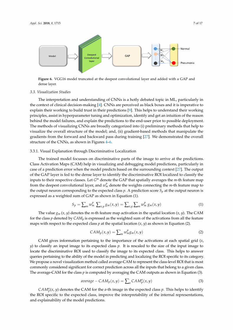
3.2.4. Customized VGG16

VGG16 is proposed and trained by the Oxford’s Visual Geometry Group (VGG) [25] for objectrecognition. The model scored first in ILSVRC image localization and second in image classificationtasks. We customized the architecture of VGG16 model and evaluated its performance toward thetasks of interest. The model is truncated at the deepest convolutional layer and added with a globalaverage pooling (GAP) and dense layer as shown in Figure 6. We refer to this model as customizedVGG16 in this study.

The hyperparameters of the customized residual, Inception and VGG16 models are optimizedthrough a randomized grid search [26] that searches and optimizes the value of hyperparametersincluding learning rate, momentum, and L2-regularization. The search ranges are initialized to[1 × 10−6 1 × 10−1], [0.7 0.99], and [1 × 10−10 1 × 10−1] for the learning rate, momentum, andL2-regularization respectively. Callbacks are used to view the internal states during training andretain the best performing model for analysis. We performed hold-out testing with the test data afterevery step. The performance of customized CNNs are evaluated in terms of the following performancemetrics: (i) accuracy; (ii) AUC; (iii) precision; (iv) recall; (v) specificity; (vi) F-Score; and, (vii) MatthewsCorrelation Coefficient (MCC). We used the NIH Biowulf Linux cluster (https://hpc.nih.gov/) andthe high performance computing facility at the National Library of Medicine (NLM) for computationalanalyses. Software frameworks included with Matlab R2017b are used to configure and evaluatethe sequential CNN along with Keras and Tensorflow backend for other customized models used inthis study.

https://hpc.nih.gov/

Appl. Sci. 2018, 8, 1715 7 of 17


Figure 6. VGG16 model truncated at the deepest convolutional layer and added with a GAP and dense layer.

3.3. Visualization Studies

The interpretation and understanding of CNNs is a hotly debated topic in ML, particularly in the context of clinical decision-making [4]. CNNs are perceived as black boxes and it is imperative to explain their working to build trust in their predictions [9]. This helps to understand their working principles, assist in hyperparameter tuning and optimization, identify and get an intuition of the reason behind the model failures, and explain the predictions to the end-user prior to possible deployment. The methods of visualizing CNNs are broadly categorized into (i) preliminary methods that help to visualize the overall structure of the model; and, (ii) gradient-based methods that manipulate the gradients from the forward and backward pass during training [27]. We demonstrated the overall structure of the CNNs, as shown in Figures 4–6.

3.3.1. Visual Explanation through Discriminative Localization

The trained model focusses on discriminative parts of the image to arrive at the predictions. Class Activation Maps (CAM) help in visualizing and debugging model predictions, particularly in case of a prediction error when the model predicts based on the surrounding context [27]. The output of the GAP layer is fed to the dense layer to identify the discriminative ROI localized to classify the inputs to their respective classes. Let Gm denote the GAP that spatially averages the m-th feature map from the deepest convolutional layer, and 𝑤 denote the weights connecting the m-th feature map to the output neuron corresponding to the expected class p. A prediction score Sp at the output neuron is expressed as a weighted sum of GAP as shown in Equation (1). 𝑆 = ∑ 𝑤 ∑ 𝑔 (𝑥, 𝑦) = ∑ ∑ 𝑤 ,, 𝑔 (𝑥, 𝑦) (1)

The value gm (x, y) denotes the m-th feature map activation in the spatial location (x, y). The CAM for the class p denoted by CAMp is expressed as the weighted sum of the activations from all the feature maps with respect to the expected class p at the spatial location (x, y) as shown in Equation (2). 𝐶𝐴𝑀 (𝑥, 𝑦) = ∑ 𝑤 𝑔 (𝑥, 𝑦) (2)

CAM gives information pertaining to the importance of the activations at each spatial grid (x, y) to classify an input image to its expected class p. It is rescaled to the size of the input image to locate the discriminative ROI used to classify the image to its expected class. This helps to answer queries pertaining to the ability of the model in predicting and localizing the ROI specific to its category. We propose a novel visualization method called average-CAM to represent the class-level ROI that is most commonly considered significant for correct prediction across all the inputs that belong to a given class. The average-CAM for the class p is computed by averaging the CAM outputs as shown in Equation (3). 𝑎𝑣𝑒𝑟𝑎𝑔𝑒 − 𝐶𝐴𝑀 (𝑥, 𝑦) = ∑ 𝐶𝐴𝑀 (𝑥, 𝑦) (3) 𝐶𝐴𝑀 (x, y) denotes the CAM for the a-th image in the expected class p. This helps to identify the ROI specific to the expected class, improve the interpretability of the internal representations, and explainability of the model predictions.

Figure 6. VGG16 model truncated at the deepest convolutional layer and added with a GAP anddense layer.

3.3. Visualization Studies

The interpretation and understanding of CNNs is a hotly debated topic in ML, particularly inthe context of clinical decision-making [4]. CNNs are perceived as black boxes and it is imperative toexplain their working to build trust in their predictions [9]. This helps to understand their workingprinciples, assist in hyperparameter tuning and optimization, identify and get an intuition of the reasonbehind the model failures, and explain the predictions to the end-user prior to possible deployment.The methods of visualizing CNNs are broadly categorized into (i) preliminary methods that help tovisualize the overall structure of the model; and, (ii) gradient-based methods that manipulate thegradients from the forward and backward pass during training [27]. We demonstrated the overallstructure of the CNNs, as shown in Figures 4–6.

3.3.1. Visual Explanation through Discriminative Localization

The trained model focusses on discriminative parts of the image to arrive at the predictions.Class Activation Maps (CAM) help in visualizing and debugging model predictions, particularly incase of a prediction error when the model predicts based on the surrounding context [27]. The outputof the GAP layer is fed to the dense layer to identify the discriminative ROI localized to classify theinputs to their respective classes. Let Gm denote the GAP that spatially averages the m-th feature mapfrom the deepest convolutional layer, and wp

m denote the weights connecting the m-th feature map tothe output neuron corresponding to the expected class p. A prediction score Sp at the output neuron isexpressed as a weighted sum of GAP as shown in Equation (1).

Sp = ∑m wpm ∑x,y gm(x, y) = ∑x,y ∑m wp

m gm(x, y) (1)

The value gm (x, y) denotes the m-th feature map activation in the spatial location (x, y). The CAMfor the class p denoted by CAMp is expressed as the weighted sum of the activations from all the featuremaps with respect to the expected class p at the spatial location (x, y) as shown in Equation (2).

CAMp(x, y) = ∑m wpmgm(x, y) (2)

CAM gives information pertaining to the importance of the activations at each spatial grid (x,y) to classify an input image to its expected class p. It is rescaled to the size of the input image tolocate the discriminative ROI used to classify the image to its expected class. This helps to answerqueries pertaining to the ability of the model in predicting and localizing the ROI specific to its category.We propose a novel visualization method called average-CAM to represent the class-level ROI that is mostcommonly considered significant for correct prediction across all the inputs that belong to a given class.The average-CAM for the class p is computed by averaging the CAM outputs as shown in Equation (3).

average− CAMp(x, y) = ∑a CAMap(x, y) (3)

CAMap(x, y) denotes the CAM for the a-th image in the expected class p. This helps to identify

the ROI specific to the expected class, improve the interpretability of the internal representations,and explainability of the model predictions.

Appl. Sci. 2018, 8, 1715 8 of 17

CAM visualization can only be applied to networks with a GAP layer. Gradient-weighted CAM(grad-CAM) is a strict generalization of CAM that can be applied to all existing CNNs [28]. It usesthe gradient information of the expected class, flowing back into the deepest convolutional layer togenerate explanations. Grad-CAM produces the weighted sum of all the feature maps in the deepestconvolutional layer for the expected class p as shown in Equation (4). A ReLU nonlinearity is appliedto avoid the negative weights from influencing the class p. This is based on the consideration that thepixels with negative weights are likely to belong to other classes.

grad− CAMp(x, y) = ReLU(∑m β

pmgm(x, y)

)(4)

The value βpm is obtained by computing the gradient of the prediction score Sp with respect to the

m-th feature map as shown in Equation (5).

βpm = ∑x,y

∂Sp

∂gm(x, y)(5)

According to Equations (1) and (4), βpm is precisely the same as wp

m for networks witha CAM-compatible architecture. The difference lies in applying the ReLU non-linearity to excludethe influence of negative weights that are likely to belong to other classes. The average-grad-CAMfor the class p is computed by averaging the grad-CAM outputs as shown in Equation (6). The valuegrad-CAMa

p(x, y) denotes the grad-CAM for the a-th image in the expected class p.

average− grad− CAMp(x, y) = ∑a

grad− CAMap(x, y) (6)

3.3.2. Model-Agnostic Visual Explanations

Local interpretable model-agnostic explanations (LIME) is a visualization tool proposed by [29].It helps to provide a qualitative interpretation of the relationship between perturbed input instancesand the model predictions. The input image is divided into contiguous superpixels and a datasetof perturbed input instances is constructed by turning on/off these interpretable components.The perturbed instances are weighted by their similarity to the explained instance. The algorithmapproximates the CNN by a sparse, linear model that is weighted only in the neighborhood of theexplained predictions. An explanation is generated in the form of superpixels with the highest positiveweights that demonstrate the discriminative ROI localized by the model to classify the image toits expected class. Let k ∈ Rd be the explained instance, and k′ ∈ {0, 1}d, the binary vector thatdenotes the presence/absence of a superpixel. Let g ∈ G denote the explanation where G is a class ofinterpretable linear models. Let


CAM visualization can only be applied to networks with a GAP layer. Gradient-weighted CAM (grad-CAM) is a strict generalization of CAM that can be applied to all existing CNNs [28]. It uses the gradient information of the expected class, flowing back into the deepest convolutional layer to generate explanations. Grad-CAM produces the weighted sum of all the feature maps in the deepest convolutional layer for the expected class p as shown in Equation (4). A ReLU nonlinearity is applied to avoid the negative weights from influencing the class p. This is based on the consideration that the pixels with negative weights are likely to belong to other classes. 𝑔𝑟𝑎𝑑 − 𝐶𝐴𝑀 (𝑥, 𝑦) = 𝑅𝑒𝐿𝑈(∑ 𝛽 𝑔 (𝑥, 𝑦)) (4)

The value 𝛽 is obtained by computing the gradient of the prediction score Sp with respect to the m-th feature map as shown in Equation (5). 𝛽 = ∑ ( , ), (5)

According to Equations (1) and (4), 𝛽 is precisely the same as 𝑤 for networks with a CAM-compatible architecture. The difference lies in applying the ReLU non-linearity to exclude the influence of negative weights that are likely to belong to other classes. The average-grad-CAM for the class p is computed by averaging the grad-CAM outputs as shown in Equation (6). The value grad-𝐶𝐴𝑀 (x, y) denotes the grad-CAM for the a-th image in the expected class p. 𝑎𝑣𝑒𝑟𝑎𝑔𝑒 − 𝑔𝑟𝑎𝑑 − 𝐶𝐴𝑀 (𝑥, 𝑦) = ∑ 𝑔𝑟𝑎𝑑 − 𝐶𝐴𝑀 (𝑥, 𝑦) (6)


Local interpretable model-agnostic explanations (LIME) is a visualization tool proposed by [29]. It helps to provide a qualitative interpretation of the relationship between perturbed input instances and the model predictions. The input image is divided into contiguous superpixels and a dataset of perturbed input instances is constructed by turning on/off these interpretable components. The perturbed instances are weighted by their similarity to the explained instance. The algorithm approximates the CNN by a sparse, linear model that is weighted only in the neighborhood of the explained predictions. An explanation is generated in the form of superpixels with the highest positive weights that demonstrate the discriminative ROI localized by the model to classify the image to its expected class. Let k ∈ ℝd be the explained instance, and k’ ∈ {0, 1}d, the binary vector that denotes the presence/absence of a superpixel. Let g ∈ G denote the explanation where G is a class of interpretable linear models. Let ℽ(g) denote the complexity measure associated with the explanation g ∈ G. The value ℽ(g) denotes the number of non-zero coefficients for the linear model. Let m: ℝd → ℝ denote the explained model and m(k), the probability that k belongs to a given class. Let Πk(x) denote the measure of proximity between the instance x to k and P(m, g, Πk) denote the loss of g toward approximating m in the neighborhood defined by Πk. The value P(m, g, Πk) is minimized and the value of ℽ(g) remains low enough for interpretability. Equation (7) gives the explanations produced by LIME. 𝛽(𝑘) = argmin ∈ 𝑃(𝑚, 𝑔, 𝛱 ) + ℽ(𝑔) (7)

The value P (m, g, Πk) is approximated by drawing samples weighted by Πk. Equation (8) shows an exponential kernel defined on the L2-distance function (J) with width €. For a given input perturbed sample b’ ∈ {0, 1}d’ containing a fraction of non-zero elements, the label for the explanation model m(b) is obtained by recovering the sample in the original representation b ∈ ℝd as shown in Equation (9). Π = exp(−𝐽 ( , )€ ) (8) 𝑃(𝑚, 𝑔, Π ) = ∑ Π (𝑚(𝑏) − 𝑔(𝑏 )), ∈ (9)

LIME provides explanations that help to make an informed decision about the trustworthiness of the predictions and gain crucial insights into the model behavior.

(g) denote the complexity measure associated with the explanationg ∈ G. The value









(g) denotes the number of non-zero coefficients for the linear model. Let m: Rd → Rdenote the explained model and m(k), the probability that k belongs to a given class. Let Πk(x) denotethe measure of proximity between the instance x to k and P(m, g, Πk) denote the loss of g towardapproximating m in the neighborhood defined by Πk. The value P(m, g, Πk) is minimized and thevalue of









(g) remains low enough for interpretability. Equation (7) gives the explanations producedby LIME.

β(k) = argming∈G

P(m, g, Πk) + (g) (7)

The value P (m, g, Πk) is approximated by drawing samples weighted by Πk. Equation (8) showsan exponential kernel defined on the L2-distance function (J) with widthe. For a given input perturbedsample b′ ∈ {0, 1}d′ containing a fraction of non-zero elements, the label for the explanation model m(b)is obtained by recovering the sample in the original representation b ∈ Rd as shown in Equation (9).

Πbk = exp

(−J

(y, b)2

e2

)(8)

Appl. Sci. 2018, 8, 1715 9 of 17

P(m, g, Πk) = ∑b,b∈B Πbk(m(b)− g

(b′))

2 (9)

LIME provides explanations that help to make an informed decision about the trustworthiness ofthe predictions and gain crucial insights into the model behavior.

4. Results and Discussion

4.1. Performance Evaluation of Customized CNNs

Figure 7 shows the optimized architecture and parameters of the sequential CNN, obtained throughBayesian learning. We performed 100 objective function evaluations toward optimizing the modelparameters. The optimized values are found to be 6, 1 × 10−3, 0.9, and 1 × 10−6 for the network depth,learning rate, momentum, and L2-regularization parameters respectively. The number of convolutionallayer filters is increased by a factor of 2 each time a max-pooling layer is used, in order to ensure roughlythe same number of computations in the network layers. Rectified Linear Unit (ReLU) layers are added tointroduce non-linearity and prevent vanishing gradients during backpropagation [7].


4. Results and Discussion

4.1. Performance Evaluation of Customized CNNs

Figure 7 shows the optimized architecture and parameters of the sequential CNN, obtained through Bayesian learning. We performed 100 objective function evaluations toward optimizing the model parameters. The optimized values are found to be 6, 1 × 10−3, 0.9, and 1 × 10−6 for the network depth, learning rate, momentum, and L2-regularization parameters respectively. The number of convolutional layer filters is increased by a factor of 2 each time a max-pooling layer is used, in order to ensure roughly the same number of computations in the network layers. Rectified Linear Unit (ReLU) layers are added to introduce non-linearity and prevent vanishing gradients during backpropagation [7].

Figure 7. The optimized architecture of customized sequential CNN.

Our analysis shows an increase in the performance of the residual and inception CNNs when the number of filters in the convolutional layers of the succeeding blocks are increased by a factor of 2. We found the optimal hyperparameter values for the residual, inception, and VGG16 models through a randomized grid search. The values are tabulated in Table 2.

Figure 7. The optimized architecture of customized sequential CNN.

Our analysis shows an increase in the performance of the residual and inception CNNs when thenumber of filters in the convolutional layers of the succeeding blocks are increased by a factor of 2.We found the optimal hyperparameter values for the residual, inception, and VGG16 models througha randomized grid search. The values are tabulated in Table 2.

The customized CNNs are evaluated with the baseline and cropped ROI data. The results aretabulated in Table 3. We observed that the performance of the models with the cropped ROI is relativelypromising in comparison to the baseline in classifying normal and pneumonia infected CXRs. This isobvious because the models trained with the cropped ROI learn relevant feature representationstoward classifying the task of interest.

Appl. Sci. 2018, 8, 1715 10 of 17

Table 2. Optimal values for the hyperparameters of the customized residual and inception CNNsobtained through a randomized grid search.

Model Learning Rate Momentum L2 Regularization

Residual CNN 1 × 10−3 0.9 1 × 10−6

Inception CNN 1 × 10−2 0.95 1 × 10−4

Customized VGG16 1 × 10−4 0.99 1 × 10−6

Table 3. Performance of customized CNNs with baseline and cropped ROI data.

Task Data Models Accuracy AUC Precision Recall Specificity F-Score MCC

Normal vs.Pneumonia

Baseline

CustomizedVGG16 0.957 0.990 0.951 0.983 0.915 0.967 0.908

Sequential 0.943 0.983 0.920 0.980 0.855 0.957 0.878Residual 0.910 0.967 0.908 0.954 0.838 0.931 0.806Inception 0.886 0.922 0.887 0.939 0.800 0.913 0.755

CroppedROI

CustomizedVGG16 0.962 0.993 0.977 0.962 0.962 0.970 0.918


Bacterial vs. ViralPneumonia

Baseline

CustomizedVGG16 0.936 0.962 0.920 0.984 0.860 0.951 0.862


CroppedROI

CustomizedVGG16 0.936 0.962 0.920 0.984 0.860 0.951 0.862


Normal vs.Bacterial vs. Viral

Pneumonia

Baseline

CustomizedVGG16 0.917 0.938 0.917 0.905 0.958 0.911 0.873


CroppedROI

CustomizedVGG16 0.918 0.939 0.920 0.900 0.960 0.910 0.876


* Bold numbers indicate superior performance.

The customized VGG16 model demonstrates promising performance than the other CNNs understudy. The model learned generic image features from ImageNet that served as a good initializationcompared to random weights and trained end-to-end on the current tasks to learn task-specificfeatures. This results in faster convergence with reduced bias, overfitting, and improved generalization.In classifying bacterial and viral pneumonia, no significant difference in performance is observed forthe customized VGG16 model with the baseline and cropped ROI. In the multi-class classification task,the cropped ROI gave better results than the baseline data. However, we observed that the differencesin performance are not significant. This may be due to the reason that the dataset under study alreadyappeared as cropped, and the boundary detection algorithm resulted in a few under-segmentedregions near the costophrenic angle. The customized sequential, residual, and inception CNNs withrandom weight initializations didn’t have the opportunity to learn discriminative features, owingto the sparse availability and imbalanced distribution of training data across the expected classes.We observed that the sequential CNN outperformed the residual and inception counterparts acrossthe classification tasks. The usage of residual connections is beneficial in resolving the issue ofrepresentational bottlenecks and vanishing gradients in deep models. The CNNs used in this studyhave a shallow architecture. The residual connections did not introduce significant gains into theperformance for the tasks of interest. Unlike ImageNet, the variability in the pediatric CXR data isseveral orders of magnitude smaller. The architecture of residual and inception CNNs are progressivelymore complex and did not seem to be a fitting tool to use for the tasks of interest. The confusion matrices

Appl. Sci. 2018, 8, 1715 11 of 17

and AUC achieved with the customized VGG16 model are shown in Figures 8–10. We observed thatthe training metrics are poor compared to test accuracy. This is due to the fact that noisy images areincluded in the training data to reduce bias, overfitting, and improve model generalization.

We compared the performance of the customized VGG16 model trained with the cropped ROI,to the state-of-the-art. The results are tabulated in Table 4. We observed that our model outperformsthe current literature in all performance metrics across the classification tasks. The customizedsequential CNN demonstrates higher values for recall in: (i) classifying normal and pneumonia;and, (ii) identical recall measures to the customized VGG16 model in classifying bacterial and viralpneumonia. However, considering the balance between precision and recall as demonstrated by theF-Score and MCC, the customized VGG16 model outperforms the other CNNs and the state-of-the-artacross the classification tasks.


inception CNNs with random weight initializations didn’t have the opportunity to learn discriminative features, owing to the sparse availability and imbalanced distribution of training data across the expected classes. We observed that the sequential CNN outperformed the residual and inception counterparts across the classification tasks. The usage of residual connections is beneficial in resolving the issue of representational bottlenecks and vanishing gradients in deep models. The CNNs used in this study have a shallow architecture. The residual connections did not introduce significant gains into the performance for the tasks of interest. Unlike ImageNet, the variability in the pediatric CXR data is several orders of magnitude smaller. The architecture of residual and inception CNNs are progressively more complex and did not seem to be a fitting tool to use for the tasks of interest. The confusion matrices and AUC achieved with the customized VGG16 model are shown in Figures 8–10. We observed that the training metrics are poor compared to test accuracy. This is due to the fact that noisy images are included in the training data to reduce bias, overfitting, and improve model generalization.

We compared the performance of the customized VGG16 model trained with the cropped ROI, to the state-of-the-art. The results are tabulated in Table 4. We observed that our model outperforms the current literature in all performance metrics across the classification tasks. The customized sequential CNN demonstrates higher values for recall in: (i) classifying normal and pneumonia; and, (ii) identical recall measures to the customized VGG16 model in classifying bacterial and viral pneumonia. However, considering the balance between precision and recall as demonstrated by the F-Score and MCC, the customized VGG16 model outperforms the other CNNs and the state-of-the-art across the classification tasks.

Figure 8. Confusion matrices for the performance of the customized VGG16 model: (a) Normal v. Pneumonia; (b) Bacterial v. Viral Pneumonia.

Figure 9. ROC curves demonstrating the performance of the customized VGG16 model: (a) Normal v. Pneumonia; (b) Bacterial v. Viral Pneumonia.

Figure 8. Confusion matrices for the performance of the customized VGG16 model: (a) Normal v.Pneumonia; (b) Bacterial v. Viral Pneumonia.


inception CNNs with random weight initializations didn’t have the opportunity to learn discriminative features, owing to the sparse availability and imbalanced distribution of training data across the expected classes. We observed that the sequential CNN outperformed the residual and inception counterparts across the classification tasks. The usage of residual connections is beneficial in resolving the issue of representational bottlenecks and vanishing gradients in deep models. The CNNs used in this study have a shallow architecture. The residual connections did not introduce significant gains into the performance for the tasks of interest. Unlike ImageNet, the variability in the pediatric CXR data is several orders of magnitude smaller. The architecture of residual and inception CNNs are progressively more complex and did not seem to be a fitting tool to use for the tasks of interest. The confusion matrices and AUC achieved with the customized VGG16 model are shown in Figures 8–10. We observed that the training metrics are poor compared to test accuracy. This is due to the fact that noisy images are included in the training data to reduce bias, overfitting, and improve model generalization.

We compared the performance of the customized VGG16 model trained with the cropped ROI, to the state-of-the-art. The results are tabulated in Table 4. We observed that our model outperforms the current literature in all performance metrics across the classification tasks. The customized sequential CNN demonstrates higher values for recall in: (i) classifying normal and pneumonia; and, (ii) identical recall measures to the customized VGG16 model in classifying bacterial and viral pneumonia. However, considering the balance between precision and recall as demonstrated by the F-Score and MCC, the customized VGG16 model outperforms the other CNNs and the state-of-the-art across the classification tasks.

Figure 8. Confusion matrices for the performance of the customized VGG16 model: (a) Normal v. Pneumonia; (b) Bacterial v. Viral Pneumonia.

Figure 9. ROC curves demonstrating the performance of the customized VGG16 model: (a) Normal v. Pneumonia; (b) Bacterial v. Viral Pneumonia.

Figure 9. ROC curves demonstrating the performance of the customized VGG16 model: (a) Normal v.Pneumonia; (b) Bacterial v. Viral Pneumonia.

Table 4. Comparing the performance of the customized VGG16 model with the state-of-the-art.

Task Model Accuracy AUC Precision Recall Specificity F-Score MCC

Normal v.Pneumonia

CustomizedVGG16 0.962 0.993 0.977 0.962 0.962 0.970 0.918

Kermany et al. 0.928 0.968 - 0.932 0.901 - -

Bacterial v. ViralPneumonia

CustomizedVGG16 0.936 0.962 0.920 0.984 0.860 0.951 0.862

Kermany et al. 0.907 0.940 - 0.886 0.909 - -

Normal v.Bacterial v. Viral

Pneumonia

CustomizedVGG16 0.918 0.939 0.920 0.900 0.960 0.910 0.876

Kermany et al. - - - - - - -


Appl. Sci. 2018, 8, 1715 12 of 17


Figure 10. Performance of customized VGG16 model in multiclass classification: (a) Confusion matrix; (b) ROC curves.

Table 4. Comparing the performance of the customized VGG16 model with the state-of-the-art.

Task Model Accuracy AUC Precision Recall Specificity F-

Score MCC

Normal v. Pneumonia Customized

VGG16 0.962 0.993 0.977 0.962 0.962 0.970 0.918

Kermany et al. 0.928 0.968 - 0.932 0.901 - -

Bacterial v. Viral Pneumonia

Customized VGG16

0.936 0.962 0.920 0.984 0.860 0.951 0.862

Kermany et al. 0.907 0.940 - 0.886 0.909 - -

Normal v. Bacterial v. Viral Pneumonia

Customized VGG16

0.918 0.939 0.920 0.900 0.960 0.910 0.876

Kermany et al. - - - - - - -


4.2. Visualization through Discriminative Localization

The customized VGG16 model has a CAM-compatible architecture owing to the presence of the GAP layer. This helps in visualizing the model predictions using both CAM and grad-CAM visualization tools. Figures 11 and 12 demonstrate the results of applying these visualizations to localize the discriminative ROI in pneumonia-infected CXRs.

Figure 10. Performance of customized VGG16 model in multiclass classification: (a) Confusion matrix;(b) ROC curves.

4.2. Visualization through Discriminative Localization

The customized VGG16 model has a CAM-compatible architecture owing to the presence ofthe GAP layer. This helps in visualizing the model predictions using both CAM and grad-CAMvisualization tools. Figures 11 and 12 demonstrate the results of applying these visualizations tolocalize the discriminative ROI in pneumonia-infected CXRs.


Figure 11. Visual explanations through gradient-based localization using CAM: (a) Input CXRs; (b) Bounding boxes localizing regions of activations; (c) CAM showing heat maps superimposed on the original CXRs; (d) Automatically segmented lung masks; (e) CAM showing heat maps superimposed on the cropped lungs.

Figure 11. Visual explanations through gradient-based localization using CAM: (a) Input CXRs;(b) Bounding boxes localizing regions of activations; (c) CAM showing heat maps superimposed on theoriginal CXRs; (d) Automatically segmented lung masks; (e) CAM showing heat maps superimposedon the cropped lungs.

Appl. Sci. 2018, 8, 1715 13 of 17


Figure 12. Visual explanations through gradient-based localization using grad-CAM: (a) Input CXRs; (b) Bounding boxes localizing regions of activations; (c) Grad-CAM showing heat maps superimposed on the original CXRs; (d) Automatically segmented lung masks; (e) Grad-CAM showing heat maps superimposed on the cropped lungs.

CXRs are fed to the trained model and the predictions are decoded. The heat maps are generated as a two-dimensional score grid, computed for each input pixel location. Pixels carrying high importance with respect to the expected class appeared bright red with distinct color transitions for varying ranges. The generated heat maps are superimposed on the original input to localize image-specific ROI. The lung masks that are generated with the boundary detection algorithm are applied to extract the localized ROI relevant to the lung regions. We observed that CAM and grad-CAM visualizations generated heat maps for the pneumonia class to highlight the visual differences in the “pneumonia-like” regions of the image.

We applied our novel method of average-CAM and average-grad-CAM to visualize the class-specific ROI, as shown in Figures 13 and 14. Lung masks are applied to the generated heat maps to localize only the ROI specific to the lung regions. We observed that the class-specific ROI localized by the average-CAM and average-grad-CAM for the viral pneumonia class follows a diffuse pattern. This is obvious for the reason that viral pneumonia manifests with diffuse interstitial patterns in both lungs [30]. For the bacterial pneumonia class, we observed that the model layers are activated on both sides of the lungs, predominantly on the upper and middle right lung lobes. This is for the reason that bacterial pneumonia manifests as lobar considerations [30]. The pneumonia dataset under study has more pediatric patients with right lobar consolidations.

Figure 12. Visual explanations through gradient-based localization using grad-CAM: (a) Input CXRs;(b) Bounding boxes localizing regions of activations; (c) Grad-CAM showing heat maps superimposedon the original CXRs; (d) Automatically segmented lung masks; (e) Grad-CAM showing heat mapssuperimposed on the cropped lungs.

CXRs are fed to the trained model and the predictions are decoded. The heat maps are generated asa two-dimensional score grid, computed for each input pixel location. Pixels carrying high importancewith respect to the expected class appeared bright red with distinct color transitions for varyingranges. The generated heat maps are superimposed on the original input to localize image-specificROI. The lung masks that are generated with the boundary detection algorithm are applied to extractthe localized ROI relevant to the lung regions. We observed that CAM and grad-CAM visualizationsgenerated heat maps for the pneumonia class to highlight the visual differences in the “pneumonia-like”regions of the image.

We applied our novel method of average-CAM and average-grad-CAM to visualize theclass-specific ROI, as shown in Figures 13 and 14. Lung masks are applied to the generated heatmaps to localize only the ROI specific to the lung regions. We observed that the class-specific ROIlocalized by the average-CAM and average-grad-CAM for the viral pneumonia class follows a diffusepattern. This is obvious for the reason that viral pneumonia manifests with diffuse interstitial patternsin both lungs [30]. For the bacterial pneumonia class, we observed that the model layers are activatedon both sides of the lungs, predominantly on the upper and middle right lung lobes. This is for thereason that bacterial pneumonia manifests as lobar considerations [30]. The pneumonia dataset understudy has more pediatric patients with right lobar consolidations.

Appl. Sci. 2018, 8, 1715 14 of 17


Figure 13. Visual explanations through average-CAM: (a) Bacterial and viral CXR (top and bottom); (b) Average-CAM localizing class-specific ROI with bounding boxes highlighting the regions of maximum activation; (c) Automatically segmented lung masks; (d) Average-CAM localizing class-specific ROI with the extracted lung regions.

Figure 14. Visual explanations through average-grad-CAM: (a) Bacterial and viral CXR (top and bottom); (b) Average-grad-CAM localizing class-specific ROI with bounding boxes highlighting the regions of maximum activation; (c) Automatically segmented lung masks; (d) Average-grad-CAM localizing class-specific ROI with the extracted lung regions.

4.3. Visual Explanations with LIME

Figure 15 shows the explanations generated with LIME for sample instances of pediatric chest radiographs. Lung masks are applied to the explanations to localize only the ROI specific to the lung regions. The explanations are shown as follows: (i) Superpixels with the highest positive weights and the rest are greyed out; and, (ii) superpixels superimposed on the extracted lung regions. We observed that the explainer focused on the regions with high opacity. The model differentiates bacterial and viral pneumonia by (i) showing superpixels with the highest positive activations in the regions of lobar consolidations for bacterial pneumonia; and, (ii) diffuse interstitial patterns across

Figure 13. Visual explanations through average-CAM: (a) Bacterial and viral CXR (top andbottom); (b) Average-CAM localizing class-specific ROI with bounding boxes highlighting the regionsof maximum activation; (c) Automatically segmented lung masks; (d) Average-CAM localizingclass-specific ROI with the extracted lung regions.


Figure 13. Visual explanations through average-CAM: (a) Bacterial and viral CXR (top and bottom); (b) Average-CAM localizing class-specific ROI with bounding boxes highlighting the regions of maximum activation; (c) Automatically segmented lung masks; (d) Average-CAM localizing class-specific ROI with the extracted lung regions.

Figure 14. Visual explanations through average-grad-CAM: (a) Bacterial and viral CXR (top and bottom); (b) Average-grad-CAM localizing class-specific ROI with bounding boxes highlighting the regions of maximum activation; (c) Automatically segmented lung masks; (d) Average-grad-CAM localizing class-specific ROI with the extracted lung regions.


Figure 15 shows the explanations generated with LIME for sample instances of pediatric chest radiographs. Lung masks are applied to the explanations to localize only the ROI specific to the lung regions. The explanations are shown as follows: (i) Superpixels with the highest positive weights and the rest are greyed out; and, (ii) superpixels superimposed on the extracted lung regions. We observed that the explainer focused on the regions with high opacity. The model differentiates bacterial and viral pneumonia by (i) showing superpixels with the highest positive activations in the regions of lobar consolidations for bacterial pneumonia; and, (ii) diffuse interstitial patterns across

Figure 14. Visual explanations through average-grad-CAM: (a) Bacterial and viral CXR (top andbottom); (b) Average-grad-CAM localizing class-specific ROI with bounding boxes highlighting theregions of maximum activation; (c) Automatically segmented lung masks; (d) Average-grad-CAMlocalizing class-specific ROI with the extracted lung regions.


Figure 15 shows the explanations generated with LIME for sample instances of pediatric chestradiographs. Lung masks are applied to the explanations to localize only the ROI specific to the lungregions. The explanations are shown as follows: (i) Superpixels with the highest positive weights andthe rest are greyed out; and, (ii) superpixels superimposed on the extracted lung regions. We observedthat the explainer focused on the regions with high opacity. The model differentiates bacterial andviral pneumonia by (i) showing superpixels with the highest positive activations in the regions of lobar

Appl. Sci. 2018, 8, 1715 15 of 17

consolidations for bacterial pneumonia; and, (ii) diffuse interstitial patterns across the lungs for viralpneumonia. We also observed that a number of false positive superpixels are reported. The reason isthat the current LIME implementation uses a sparse linear model to approximate the model behaviorin the neighborhood of the explained predictions. However, these explanations result from a randomsampling process and are not faithful if the underlying model is highly non-linear in the localityof predictions.


the lungs for viral pneumonia. We also observed that a number of false positive superpixels are reported. The reason is that the current LIME implementation uses a sparse linear model to approximate the model behavior in the neighborhood of the explained predictions. However, these explanations result from a random sampling process and are not faithful if the underlying model is highly non-linear in the locality of predictions.

Figure 15. Visual explanations through LIME: (a) Input CXRs; (b) Automatically segmented lung masks; (c) Copped lung regions; (d) Superpixels with the highest positive weights with the others greyed out; (e) Superpixels with the highest positive weights are superimposed on the cropped lungs.

5. Conclusions

We proposed a CNN-based decision support system to detect pneumonia in pediatric CXRs to expedite accurate diagnosis of the pathology. We applied novel and state-of-the-art visualization strategies to explain model predictions that is considered highly significant to clinical decision-making. The study presents a universal approach to apply to an extensive range of visual recognition tasks. Classifying pneumonia in chest radiographs is a demanding task due to the presence of a high degree of variability in the input data. The promising performance of the customized VGG16 model trained on the current tasks suggest that it effectively learns from a sparse collection of complex data with reduced bias and improved generalization. We hope that our results are useful for developing clinically useful solutions to detect and distinguish pneumonia types in chest radiographs.

Author Contributions: Conceptualization, S.R. and S.A.; Methodology, S.R.; Software, S.R., S.C., and I.K.; Validation, S.R., S.C., and I.K.; Formal Analysis, S.R.; Investigation, S.R., and S.A.; Resources, S.R. and S.C.; Data Curation, S.R.; Writing-Original Draft Preparation, S.R.; Writing-Review & Editing, S.A. and G.T.; Visualization, S.R.; Supervision, S.A. and G.T.; Project Administration, S.A. and G.T.; Funding Acquisition, S.A. and G.T.

Figure 15. Visual explanations through LIME: (a) Input CXRs; (b) Automatically segmented lungmasks; (c) Copped lung regions; (d) Superpixels with the highest positive weights with the othersgreyed out; (e) Superpixels with the highest positive weights are superimposed on the cropped lungs.

5. Conclusions

We proposed a CNN-based decision support system to detect pneumonia in pediatric CXRs toexpedite accurate diagnosis of the pathology. We applied novel and state-of-the-art visualizationstrategies to explain model predictions that is considered highly significant to clinical decision-making.The study presents a universal approach to apply to an extensive range of visual recognition tasks.Classifying pneumonia in chest radiographs is a demanding task due to the presence of a high degreeof variability in the input data. The promising performance of the customized VGG16 model trainedon the current tasks suggest that it effectively learns from a sparse collection of complex data withreduced bias and improved generalization. We hope that our results are useful for developing clinicallyuseful solutions to detect and distinguish pneumonia types in chest radiographs.

Author Contributions: Conceptualization, S.R. and S.A.; Methodology, S.R.; Software, S.R., S.C., and I.K.;Validation, S.R., S.C., and I.K.; Formal Analysis, S.R.; Investigation, S.R., and S.A.; Resources, S.R. and S.C.; Data

Appl. Sci. 2018, 8, 1715 16 of 17

Curation, S.R.; Writing-Original Draft Preparation, S.R.; Writing-Review & Editing, S.A. and G.T.; Visualization,S.R.; Supervision, S.A. and G.T.; Project Administration, S.A. and G.T.; Funding Acquisition, S.A. and G.T.

Funding: This work was supported by the Intramural Research Program of the Lister Hill National Center forBiomedical Communications (LHNCBC), the National Library of Medicine (NLM), and the U.S. National Institutesof Health (NIH).

Conflicts of Interest: The authors declare no conflict of interest.

References

1. Le Roux, D.M.; Myer, L.; Nicol, M.P. Incidence and severity of childhood pneumonia in the first year of lifein a South African birth cohort: The Drakenstein Child Health Study. Lancet Glob. Health 2015, 3, e95–e103.[CrossRef]

2. Mcluckie, A. Respiratory Disease and Its Management, 1st ed.; Springer: London, UK, 2009; pp. 51–59.ISBN 978-1-84882-094-4.

3. Cherian, T.; Mulholland, E.K.; Carlin, J.B.; Ostensen, H.; Amin, R.; De Campo, M.; Greenberg, D.; Lagos, R.;Lucero, M.; Madhi, S.A.; et al. Standardized interpretation of paediatric chest radiographs for the diagnosisof pneumonia in epidemiological studies. Bull. World Health Organ. 2005, 83, 353–359. [PubMed]

4. Wang, X.; Peng, Y.; Lu, L.; Lu, Z.; Bagheri, M.; Summers, R.M. ChestX-Ray8: Hospital-Scale Chest X-RayDatabase and Benchmarks on Weakly-Supervised Classification and Localization of Common ThoraxDiseases. In Proceedings of the IEEE Conference on Computer Vision and Pattern Recognition (CVPR),Honolulu, HI, USA, 21–26 July 2017; pp. 3462–3471.

5. Karargyris, A.; Siegelman, J.; Tzortzis, D.; Jaeger, S.; Candemir, S.; Xue, Z.; KC, S.; Vajda, S.; Antani, S.K.;Folio, L.; et al. Combination of texture and shape features to detect pulmonary abnormalities in digital chestX-rays. Int. J. Comput. Assist. Radiol. Surg. 2016, 11, 99–106. [CrossRef] [PubMed]

6. Neuman, M.I.; Lee, E.Y.; Bixby, S.; Diperna, S.; Hellinger, J.; Markowitz, R.; Servaes, S.; Monuteaux, M.C.;Shah, S.S. Variability in the Interpretation of Chest Radiographs for the Diagnosis of Pneumonia in Children.J. Hosp. Med. 2012, 7, 294–298. [CrossRef] [PubMed]

7. Krizhevsky, A.; Sutskever, I.; Hinton, G.E. Imagenet classification with deep convolutional neural networks.In Proceedings of the Advances in Neural Information Processing Systems (NIPS), Lake Tahoe, NV, USA,3–6 December 2012; pp. 1097–1105.

8. Deng, J.; Dong, W.; Socher, R.; Li, L.J.; Li, K.; Li, F.F. ImageNet: A Large-Scale Hierarchical Image Database.In Proceedings of the IEEE Computer Society Conference on Computer Vision and Pattern Recognition(CVPR), Miami, FL, USA, 20–25 June 2009; pp. 248–255.

9. Zeiler, M.D.; Fergus, R. Visualizing and understanding convolutional networks. In Proceedings of theEuropean Conference on Computer Vision (ECCV), Zurich, Switzerland, 6–12 September 2014; Springer:Cham, Switzerland, 2014; pp. 818–833.

10. Bar, Y.; Diamant, I.; Wolf, L.; Lieberman, S.; Konen, E.; Greenspan, H. Chest Pathology Detection Using DeepLearning with Non-Medical Training. In Proceedings of the IEEE International Symposium on BiomedicalImaging (ISBI), Brooklyn, NY, USA, 16–19 April 2015; pp. 294–297.

11. Oliveira, L.L.G.; Silva, S.A.E.; Ribeiro, L.H.V.; De Oliveira, R.M.; Coelho, C.J.; Ana Lúcia, A.L.S. Computer-AidedDiagnosis in Chest Radiography for Detection of Childhood Pneumonia. Int. J. Med. Inform. 2008, 77, 555–564.[CrossRef] [PubMed]

12. Abe, H.; Macmahon, H.; Shiraishi, J.; Li, Q.; Engelmann, R.; Doi, K. Computer-aided diagnosis in chestradiology. Semin. Ultrasound CT MR 2004, 25, 432–437. [CrossRef] [PubMed]

13. Giger, M.; MacMahon, H. Image processing and computer-aided diagnosis. Radiol. Clin. N. Am. 1996,34, 565–596. [PubMed]

14. Monnier-Cholley, L.; MacMahon, H.; Katsuragawa, S.; Morishita, J.; Ishida, T.; Doi, K. Computer-aided diagnosisfor detection of interstitial opacities on chest radiographs. AJR Am. J. Roentgenol. 1998, 171, 1651–1656. [CrossRef][PubMed]

15. Kermany, D.S.; Goldbaum, M.; Cai, W.; Valentim, C.C.S.; Liang, H.; Baxter, S.L.; McKeown, A.; Yang, G.;Wu, X.; Yan, F.; et al. Identifying Medical Diagnoses and Treatable Diseases by Image-Based Deep Learning.Cell 2018, 172, 1122–1131. [CrossRef] [PubMed]

http://dx.doi.org/10.1016/S2214-109X(14)70360-2

http://www.ncbi.nlm.nih.gov/pubmed/15976876

http://dx.doi.org/10.1007/s11548-015-1242-x


http://dx.doi.org/10.1002/jhm.955


http://dx.doi.org/10.1016/j.ijmedinf.2007.10.010


http://dx.doi.org/10.1053/j.sult.2004.02.004



http://dx.doi.org/10.2214/ajr.171.6.9843307


http://dx.doi.org/10.1016/j.cell.2018.02.010


Appl. Sci. 2018, 8, 1715 17 of 17

16. Rajpurkar, P.; Irvin, J.; Zhu, K.; Yang, B.; Mehta, H.; Duan, T.; Ding, D.; Bagul, A.; Langlotz, C.; Shpanskaya, K.;et al. CheXNet: Radiologist-Level Pneumonia Detection on Chest X-Rays with Deep Learning. arXiv. 2018.Available online: https://arxiv.org/abs/1711.05225 (accessed on 23 January 2018).

17. Guan, Q.; Huang, Y.; Zhong, Z.; Zheng, Z.; Zheng, L.; Yang, Y. Diagnose like a Radiologist: AttentionGuided Convolutional Neural Network for Thorax Disease Classification. arXiv. 2018. Available online:https://arxiv.org/abs/1801.09927v1 (accessed on 17 June 2018).

18. Candemir, S.; Jaeger, S.; Palaniappan, K.; Musco, J.P.; Singh, R.K.; Xue, Z.; Karargyris, A.; Antani, S.;Thoma, G.; McDonald, C.J. Lung Segmentation in Chest Radiographs Using Anatomical Atlases withNonrigid Registration. IEEE Trans. Med. Imaging 2014, 33, 577–590. [CrossRef] [PubMed]

19. Candemir, S.; Antani, S.; Jaeger, S.; Browning, R.; Thoma, G. Lung Boundary Detection in Pediatric ChestX-Rays. In Proceedings of the SPIE Medical Imaging, Orlando, FL, USA, 21–26 February 2015; Volume 9418,p. 94180Q.

20. Liu, C.; Yuen, J.; Torralba, A. SIFT Flow: Dense Correspondence across Scenes and Its Applications.IEEE Trans. Pattern Anal. Mach. Intell. 2011, 33, 978–994. [CrossRef] [PubMed]

21. Snoek, J.; Rippel, O.; Adams, R.P. Scalable Bayesian Optimization Using Deep Neural Networks. In Proceedingsof the International Conference on Machine Learning (ICML), Lille, France, 6–11 July 2015; pp. 2171–2180.

22. Deep Learning Using Bayesian Optimization. Available online: https://www.mathworks.com/help/nnet/examples/deep-learning-using-bayesian-optimization.html (accessed on 14 January 2018).

23. He, K.; Zhang, X.; Ren, S.; Sun, J. Deep Residual Learning for Image Recognition. In Proceedings of the IEEEConference on Computer Vision and Pattern Recognition (CVPR), Las Vegas, NV, USA, 27–30 June 2016;pp. 770–778.

24. Szegedy, C.; Vanhoucke, V.; Ioffe, S.; Shlens, J.; Wojna, Z. Rethinking the Inception Architecture for ComputerVision. In Proceedings of the IEEE Conference on Computer Vision and Pattern Recognition (CVPR),Las Vegas, NV, USA, 27–30 June 2016; pp. 2818–2826.

25. Simonyan, K.; Zisserman, A. Very deep convolutional networks for large-scale image recognition. InProceedings of the 3rd International Conference on Learning Representations (ICLR), San Diego, CA, USA,7–9 May 2015; pp. 1–32.

26. Bergstra, J.; Bengio, Y. Random Search for Hyper-Parameter Optimization. JMLR 2012, 13, 281–305.27. Zhou, B.; Khosla, A.; Lapedriza, A.; Oliva, A.; Torralba, A. Learning Deep Features for Discriminative

Localization. In Proceedings of the IEEE Conference on Computer Vision and Pattern Recognition (CVPR),Las Vegas, NV, USA, 27–30 June 2016; pp. 2921–2929.

28. Selvaraju, R.R.; Cogswell, M.; Das, A.; Vedantam, R.; Parikh, D.; Batra, D. Grad-CAM: Visual Explanationsfrom Deep Networks via Gradient-Based Localization. In Proceedings of the IEEE International Conferenceof Computer Vision (ICCV), Venice, Italy, 22–29 October 2017; pp. 618–626.

29. Ribeiro, M.T.; Singh, S.; Guestrin, C. “Why Should I Trust You?”: Explaining the Predictions of Any Classifier.In Proceedings of the 22nd ACM SIGKDD International Conference on Knowledge Discovery and DataMining (KDD), San Francisco, CA, USA, 13–17 August 2016; pp. 1135–1144.

30. Sharma, S.; Maycher, B.; Eschun, G. Radiological imaging in pneumonia: Recent innovations. Curr. Opin.Pulm. Med. 2007, 13, 159–169. [CrossRef] [PubMed]

© 2018 by the authors. Licensee MDPI, Basel, Switzerland. This article is an open accessarticle distributed under the terms and conditions of the Creative Commons Attribution(CC BY) license (http://creativecommons.org/licenses/by/4.0/).

https://arxiv.org/abs/1711.05225

https://arxiv.org/abs/1801.09927v1

http://dx.doi.org/10.1109/TMI.2013.2290491


http://dx.doi.org/10.1109/TPAMI.2010.147


https://www.mathworks.com/help/nnet/examples/deep-learning-using-bayesian-optimization.html

https://www.mathworks.com/help/nnet/examples/deep-learning-using-bayesian-optimization.html

http://dx.doi.org/10.1097/MCP.0b013e3280f3bff4


http://creativecommons.org/

http://creativecommons.org/licenses/by/4.0/.

visualization and interpretation of convolutional neural ...and/or convolutional neural network...

Documents